Phase diagram of generalized TASEP on an open chain: Liggett-like boundary conditions

Abstract

The totally asymmetric simple exclusion process with generalized update is a version of the discrete time totally asymmetric exclusion process with an additional inter-particle interaction that controls the degree of particle clustering. Though the model was shown to be integrable on the ring and on the infinite lattice, on the open chain it was studied mainly numerically, while no analytic results existed even for its phase diagram. In this paper we introduce new boundary conditions associated with the infinite translation invariant stationary states of the model, which allow us to obtain the exact phase diagram analytically. We discuss the phase diagram in detail and confirm the analytic predictions by extensive numerical simulations.

I Introduction

The asymmetric simple exclusion process (ASEP) is the paradigmatic model of the non-equilibrium statistical physics. It captures main features of a variety of driven diffusive systems and has plenty of applications to many phenomena from traffic flows to interface growth as well as to transport in biological and chemical systems, [1, 2, 3]. Being a toy model, it nevertheless plays a key role as a laboratory for studies of non-equilibrium stationary states [4], boundary induced phase transitions [5]and Kardar-Parisi-Zhang theory of universal fluctuations and correlations in driven stochastic systems [6].

ASEP is a system of particles on a one-dimensional lattice performing stochastic jumps to nearest neighbor sites subject to exclusion interaction. The model was first proposed in a biological context to model the mRNA translation in protein synthesis in 1968 [7]. Two years later it was introduced in mathematical literature as a model of interacting Markov processes [8]. Since then ASEP was a subject of numerous studies. Detailed results were obtained on its stationary state in finite periodic and infinite systems as well as on a finite segment with open boundaries connected to particle reservoirs. Also, the non-stationary dynamics was analyzed in the infinite system and on the ring. Since the list of references is more than extensive, we will not give a detailed account of it here. The main ideas can be learned from reviews [9, 10, 11, 12, 13] and the details can be found in the references therein. The key reason why so many results could be obtained was a special integrable mathematical structure of the model that makes such tools as Bethe ansatz and matrix product ansatz (MPA) applicable to obtaining the exact solutions of the model [14].

Originally the model was formulated in continuous time. Also several discrete time generalizations of TASEP, the totally asymmetric version of ASEP, were proposed. Being stochastic cellular automata they suit well for computer simulations and were extensively used e.g. for modeling traffic flows. Though continuous time models are simpler to analyze, their discrete time descendants having richer dynamics allow testing the universality of results obtained for continuous time models. Different versions of discrete time TASEP use different update procedures, e.g. random, backward and forward sequential, parallel and sub-lattice parallel updates [15, 16, 17, 18]. The stationary states on a ring and on a segment were constructed for all these cases, see [19] for review and references therein. Qualitatively the large scale pictures obtained from studies of continuous and discrete time TASEPs are similar, despite the difference in their exact steady states. How an inclusion of new types of interactions into the dynamics affects the typical behavior of the system is an interesting problem and in particular is a motivation for the present work.

In this paper we focus on the stationary state of a generalization of discrete time TASEPs, TASEP with generalized update (gTASEP), considering it on a segment with open boundary conditions (BC). The difference of gTASEP from the usual discrete time TASEPs is the presence of an extra interaction controlling the particle clustering. When the parameter responsible for the interaction (probability of catching up the particle ahead) is varying from zero to one, the model crosses over from TASEP with parallel update through TASEP with backward sequential update to the deterministic aggregation regime in which particles irreversibly aggregate to giant clusters, each moving as a single particle.

The addition of extra interaction into TASEP dynamics can be useful for applications as it provides more flexibility in the modeling real life phenomena, while retaining the advantage of the model being exactly solvable. In particular, while TASEP is commonly used as one of basic models for traffic flow in a single-lane roadway [20, 3], gTASEP allows new aspects of drivers’ behavior to be taken into account. Similar issues are widely studied in the framework of so-called “car-following” models of traffic (for recent reviews see e.g. [21, 22]), which include a set of parameters like maintaining appropriate gap, speed adoption, desired acceleration or deceleration, etc., used for more realistic description of real traffic systems. Similarly, the additional interaction in gTASEP allows a study of traffic flow in different regimes, from a “repulsive”, when a car is lagging behind the car ahead, to an “attractive”, when the drivers tend to catch up with the car ahead trying to maintain the same speed as that car. Thus, clusters of synchronously moving cars may appear, leading to higher throughput. In the limiting case of irreversible aggregation the clusters of simultaneously moving cars, move forward as a whole entity. This is a simplified picture of synchronously moving vehicles in a jam.

Also, gTASEP is one of the simplest models, which allows a study of the aggregation-fragmentation processes in one dimension [23, 24]. Depending on the nature of particles, they may attract or repel each other (if e.g. they are charged), or they may be neutral. The examples of physical systems in nature, in which competing aggregation and fragmentation subject to diffusion play a major role, like e.g. reversible polymerization in solutions [25] and coagulation of colloidal particles [26], are numerous appearing in chemistry, biology and physics.

gTASEP was first proposed in [27] as a generalized version of TASEP that can be mapped to a zero-range type model with factorized steady state. This mapping allowed a study of translation invariant stationary states on a ring and its limit to the infinite system. Later, it was rediscovered as a Bethe ansatz solvable two-parameter generalization of TASEP [28] and as a particular limit of more general integrable three parametric chipping model [29]. It also appeared in the studies of the Schur measures related to deformations of the Robinson-Schensted-Knuth dynamics [30]. The integrable structure of the process allowed obtaining exact solutions for the stationary state and for the current large deviations on the finite periodic lattice [31] as well as for the non-stationary dynamics on the infinite lattice [32, 30]. In particular, these studies revealed the crossover from the Kardar-Parisi-Zhang universality class to the deterministic aggregation regime that takes place on the diffusive scale.

Yet, gTASEP in a finite system with open BC has still resisted an exact analytic treatment. Note that the stationary state of driven diffusive systems connected to particle reservoirs is usually highly nontrivial. The first exact solution for the stationary state of TASEP on an open chain was found using recursion relations between the steady states in systems of different sizes [33]. This solution inspired a discovery of the matrix product method [34] that received tremendously wide range of applications and became a basic tool for exact construction of stationary states of non-equilibrium lattice gases [35]. In particular, following the solution of the continuous time model [34, 36] the stationary states of discrete time TASEPs with parallel and ordered sequential updates were obtained [19, 17, 18]. Using these solutions exact phase diagrams were constructed.

No any such results are available for gTASEP. An attempt [37] of finding the matrix product steady state for it led only to the trivial two-dimensional representation of the bulk matrix algebra that produced the known Ising-like stationary measure on the ring [31]. On the open chain extensive numerical simulations supported with random walk based heuristic arguments were used to study the deterministic aggregation limit of the model [24, 23] as well as the whole phase diagram [38], for which, however, no any conclusive analytic predictions were still made. In this paper we make the first step in this direction obtaining conjecturally exact formulas for the phase diagram of gTASEP on a finite segment with the so called Liggett-like BC introduced below.

Introduction of these new BC to gTASEP is the key idea of the present paper. Roughly, they are defined in such a way that the particle injection to and ejection from the system at the ends of the finite lattice have the same probabilities as similar particle jumps in the infinite translation invariant stationary states of gTASEP. The structure of such stationary states parameterized by the density of particles is known and can be analyzed with usual statistical physics toolbox. In this way we can identify the so-called high and low density phases, governed by the particle injection and ejection respectively, and construct the phase diagram of the model using purely hydrodynamic arguments.

The paper is organized as follows. In section II we define the model including the new rule of the update of boundary site, which is the key formula of the present paper. In section III we describe a typical phase diagram of usual TASEP previously obtained from exact solutions, explain how it can be obtained for TASEP with Liggett-like BC from the known structure of the stationary state using only hydrodynamic arguments and outline the further steps of the same program applied to gTASEP. In section IV we describe the stationary state of gTASEP on the ring of finite size, which is then assumed to grow to infinity, and calculate probabilities of events that should mimic the particle injection to and ejection from the finite system. Using the formulas obtained we construct the phase diagram in section V. The results of numerical simulations and their comparison with those for gTASEP with the previously studied version of boundary update rules are presented in section VI. We make a few concluding comments and discuss the perspectives in section VII.

II Definition of the model

Let us consider a 1D lattice $\mathcal{L}=\{1,\dots,L\}$ with $L$ sites or the infinite lattice $\mathcal{L}=\mathbb{Z}$. A configuration $\boldsymbol{\tau}=\{\tau_{i}\}_{i\in\mathcal{L}}\in\{0,1\}^{\mathcal{L}}$ of gTASEP is a binary string of occupation numbers, which take the values $\tau_{i}=1$ if site $i$ is occupied by a particle and $\tau_{i}=0$ if it is empty. gTASEP evolves in discrete time. At every time step the whole particle configuration is updated using so called cluster-wise sequential update. By particle cluster we mean a sub-string $(\dots 01^{n}0\dots)$ of $n\geq 1$ consecutive sites filled with particles surrounded by two empty sites on both sides. The clusters of this form are referred to as bulk clusters. If we consider the finite lattice with open boundary conditions, also boundary clusters of the forms $(1^{n}0\dots)$ and $(\dots 01^{n})$ with $n\geq 1$ may exist. In them the empty site that would fall beyond left or right boundary respectively is omitted. The cluster that touches both boundaries completely fills the whole lattice being left and right boundary cluster simultaneously. Then, no bounding empty sites are assumed.

II.1 Bulk dynamics

The cluster-wise sequential update procedure is as follows, see Fig. 1.

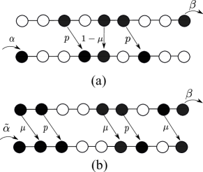
Figure 1: Two instances of gTASEP configuration updates having probabilities (a) $\alpha p^{2}(1-\mu)\beta$ and (b) $\tilde{\alpha}p^{2}\mu^{3}\beta$. A particle jumps from a lattice site to the next site on the right with probability $p$ or stays with probability $(1-p)$ if the target site was empty before the update. The probabilities change to $\mu$ and $(1-\mu)$ respectively if the target site has emptied at the same step. Similarly in (a) a particle enters to the leftmost site that was empty before the update with probability $\alpha$ and in (b) the probability is $\tilde{\alpha}$, since the site was occupied. The particle in the rightmost site leaves the lattice with probability $\beta$.

At every time step, all clusters are updated simultaneously and independently according to the following rules. From a bulk cluster the rightmost particle jumps to the next site on the right with probability $0<p\leq 1$. If the rightmost particle has jumped, the next one jumps with probability $0\leq\mu\leq 1$, and so does every next particle within the cluster provided that the previous particle has jumped. The update of the cluster ends either when one of its particles has decided not to jump or all particles of the cluster has moved one step to the right.

In other words, given a cluster $(\dots 01^{n}0\dots)$ with $n$ particles, its $0\leq m\leq n$ rightmost particles move a step to the right,

$$(\dots 01^{n}0\dots)\to(\dots 01^{n-m}01^{m}\dots),$$

with probability

$$\varphi(m|n)=\frac{v(m)w(n-m)}{f(n)},$$ (1)

defined in terms of two functions

$$v(k) = \mu^{k}(\delta_{k,0}+(1-\delta_{k,0})(1-\nu/\mu)),$$ (2)

$$w(k) = \delta_{k,0}+(1-\delta_{k,0})(1-\mu),$$ (3)

were, we have introduced yet another parameter $\nu$ related to $p$ and $\mu$ by identity

$$p=\frac{\mu-\nu}{1-\nu}.$$

The denominator

$$f\left(n\right)=\sum_{i=0}^{n}v(i)w(n-i),$$ (4)

is the normalization factor given by

$$f\left(n\right)=\delta_{n,0}+(1-\delta_{n,0})(1-\nu).$$ (5)

For $p,\mu$ to be probabilities, $0\leq p,\mu\leq 1$, parameter $\nu$ should take values in the range $\text{$\nu\leq\mu$}.$ Substituting $m=0,1,\dots,n$ into (2-5) one can directly check that these formulas are consistent with the dynamical rules described in the beginning of the section.

The form (1) of the hopping probabilities comes from [39], where it was shown to be a necessary and sufficient condition of the factorized form of the stationary probability in the so-called chipping model with zero range interaction on the ring. In that model an arbitrary number of particles in a site is allowed and $\varphi(m|n)$ is a probability for $m$ particles to jump out of a site with $n$ particles to the next site on the right. Models of this type (ZRP-like) can be related to TASEP-like models, in which a site can be occupied by at most one particle, by the so-called ZRP-ASEP mapping that replaces a cluster of particles with a single site with the same number of particles, while the one-step move of a part of the cluster to the right corresponds to the jump of as many particles to the next site. This mapping was first used to study the stationary state of the discrete time TASEP [16] and gTASEP [27] on the ring.

In formulas (1-5) specifying probabilities $\varphi(m|n)$ of gTASEP one can recognize a particular $q=0$ limit of jumping probabilities of the integrable chipping model introduced in [29] in the search for the Bethe ansatz solvable version of zero range chipping model from [39], also studied in [40] under the name $q-$Hahn TASEP. The notation $p_{m}$ for the probability $\mu$ of catching up the particle ahead was also used in [41, 24, 23, 38]. Here we keep to $p,\mu,\nu$ notations of [29, 31].

The bulk rules described specify completely the update procedure of gTASEP on the finite lattice with periodic boundary conditions, $\tau_{i}\equiv\tau_{i+L}$, and on the infinite lattice. In particular, $\mu=0$ and $\mu=p$ limits reproduce the rules of usual TASEP with parallel update (PU) and backward sequential update (BSU) respectively. In both cases all particles jump with the same probability $p$, with the sites being updated simultaneously in the former case and sequentially from right to left in the latter. We also refer to the cases $\mu<p$ and $\mu>p$ as repulsion and attraction regimes, since the particle clustering in the stationary infinite system decreases and increases respectively comparing to the independent Bernoulli stationary state with the same density of the $p=\mu$ BSU case (See [31] and discussion in the following sections).

The $\mu=1$ limit is the deterministic aggregation regime, in which particles that once got into the same cluster never split up, while the clusters themselves move as isolated particles and, when they meet, merge into bigger clusters.

Note that the cluster-wise update defined coincides with the familiar BSU prescription in many cases, e.g. in the infinite system with particle configurations bounded from the right as well as in the finite chain with open BC considered below. However, we prefer to use this formulation, because of subtleties which appear e.g. on the ring, where an ambiguity in the choice of the starting point of update exists. Also, we recall that TASEP-like models with such an update are mapped under the ZRP-ASEP mapping to the chipping models with zero-range interaction and parallel update from [39], which become tractable, when the hopping probabilities have the form (1).

II.2 Boundary dynamics

If gTASEP is considered on the finite segment, the updates of the boundary clusters should be defined separately. We will assume that particles may be added into the system at the leftmost site, $i=1$, of the lattice and removed from the system from the last site, $i=L$. On the update of the boundary cluster near the right boundary the particle at site $i=L$ is removed with probability $\beta$. If this has happened and the cluster consists of more than one particle, the next particle makes a step to the emptied site with probability $\mu$ and so does the next particle, etc, until either all particles of the cluster have made a step or some particle decides not to jump with probability $(1-\mu)$. Thus, the possible outcomes of an update of the right boundary cluster with $n\geq 1$ particles have the following probabilities

$$(\dots 01^{n})\to(\dots 01^{n}): \,1-\beta,n\geq 1;$$

$$(\dots 01^{n})\!\to\!(\dots 01^{n-m}01^{m-1}): \,\beta\mu^{m-1}(1-\mu),1\leq m<n;$$

$$(\dots 01^{n})\to(\dots 001^{n-1}): \,\beta\mu^{n-1}.$$

How is the left boundary updated? If the leftmost site, $i=1$, of the lattice was empty before the update, a particle is added to this site with probability $0<\alpha\leq 1$, so that the left boundary cluster appears. If the left boundary cluster existed, it is updated in the same way as the bulk cluster. If the leftmost site $i=1$ has emptied as a result of this update, a particle may be added there with yet another probability

$$\tilde{\alpha}=\frac{\alpha\mu}{\mu-(1-\alpha)\nu}=\frac{\alpha\mu(1-p)}{\alpha(\mu-p)+p(1-\mu)}.$$ (6)

Then the updates of the left boundary with corresponding probabilities are

$$(0\dots)\to(1\dots) :\,\alpha;$$

$$(0\dots)\to(0\dots) :\,1-\alpha;$$

$$(1^{n}0\dots)\to(1^{n}0\dots) :\,1-p,1\leq n;$$

$$(1^{n}0\dots)\to(1^{n-m}01^{m}\dots) :\,p\mu^{m-1}(1-\mu),1\leq m<n;$$

$$(1^{n}0\dots)\to(01^{n}\dots) :\,p\mu^{m-1}(1-\tilde{\alpha}),1\leq n;$$

$$(1^{n}0\dots)\to(1^{n+1}\dots) :\,p\mu^{n-1}\tilde{\alpha},m<n.$$

If the cluster to be updated fills the whole lattice, the probabilities are prescribed in the same way as to the update of the left boundary cluster up to the change of the first particle jump probability $p$ to $\beta$.

Relation (6) between $\alpha,\tilde{\alpha}$ and the bulk jump probabilities $p,\mu$ is the key formula of the present paper. Given here as a definition, it will be derived below from the assumption that the injection probabilities coincide with the probabilities of similar particle jumps in the infinite stationary translation invariant system. One can see that given fixed values of $p$ and $\mu$, parameter $\tilde{\alpha}$ is the monotonous function of $\alpha$ taking values in the range

$$0\leq\tilde{\alpha}\leq 1$$

as $\alpha$ varies in the same range. Furthermore, as will be explained below, when the values of $\alpha$ vary in the range

$$0<\alpha\leq p,$$

and consequently, $\tilde{\alpha}$ following (6) takes values in

$$0\leq\tilde{\alpha}\leq\mu,$$

these parameters can be associated with the stationary state of the infinite translation invariant system with the same bulk dynamics at some particle density value. The same applies to the right boundary condition with parameter $\beta$ in the rage $0\leq\beta\leq p$. Thus, we refer to so defined boundary dynamics as Liggett-like BC. All the results obtained below for gTASEP on a segment are the consequence of this definition.

In particular cases of PU and BSU bulk dynamics, corresponding to $\mu=0$ and $\mu=p$ respectively, we find $\tilde{\alpha}=0$ and $\tilde{\alpha}=\alpha$, the values that reproduce the corresponding BC that were used in the previous exact solutions of those models. We would expect that the choice (6) would also be in some sense good, i.e. potentially exactly solvable.

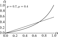
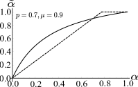
(a)                            (b)

Figure 2: Typical plots of $\tilde{\alpha}$ vs $\alpha$ in (a) attracting, $p<\mu$, and (b) repulsive, $p>\mu$, regimes for two definitions of $\tilde{\alpha}$: formula (6) – solid curves, and formula (7) – dashed curves.

The formula (6) is to be compared with another choice of formula

$$\tilde{\alpha}=\min(1,\alpha\mu/p)$$ (7)

proposed in [42, 24]. This prescription also matches with the of PU and BSU cases. However, in general it is not clear how to associate such BC with the fixed density reservoir, which makes the analysis of phase diagram a more difficult problem.

To compare them qualitatively, we note that at fixed $p>\mu$ ($p<\mu$) $\tilde{\alpha}$ defined by (6) is a monotonously increasing convex (concave) function of $\alpha$. Its plot has a unique common point with the piece-wise linear function (7) in the interval $\alpha\in(0,1)$ at $\alpha=p$. Thus, in the repulsive regime, $p>\mu$, the effective flow into the system with BC (6) is enhanced compared to the that with BC (7) when $\alpha<p$ and suppressed when $\alpha>p$ and vice versa in the attractive regime, $p<\mu$, see fig. 2. Below will see numerical consequences of this fact.

III Phase diagram of TASEP

Before describing our results let us informally discuss how the known phase diagrams obtained from exact solutions of the usual TASEP typically look like and what is the significance of the Liggett-like BC. The examples, which we keep in mind, are the discrete time TASEPs with BSU and PU, obtained from the above defined gTASEP by setting $\mu=p$ and $\mu=0$ respectively, and the continuous time TASEP that can be obtained from both discrete time cases in $p\to 0$ limit.

In the usual continuous (discrete) time TASEPs all particles on a 1D lattice jump in one direction with same unit rate (probability $p$) subject to the exclusion interaction. Also boundary rates (probabilities), $\alpha,\beta$, which are in general different from the bulk one, are assigned to particle injection to the first site of the chain and particle ejection from the last site of the chain, which also happen according to the same update. This is the simplest and most natural choice of BC.

By luck, in a suitable range of $\alpha,\beta$ so introduced BC, are the examples of the BC introduced by Liggett [43, 44]. They imply that the leftmost (rightmost) site of the segment is attached to a reservoir, which is the left (right) half of a 1D infinite system with the same TASEP being in the translation invariant steady state with fixed particle density value related to the value of boundary parameter $\alpha$ ($\beta$). (Note that every mentioned version of TASEP on the infinite chain has a family of rather simple translation invariant steady states parameterized by the value of particle density. These are product of independent Bernoulli measures in continuous time as well as the BSU case and 1D Ising-like measure in the PU case.) Obviously, when the densities of the right and left reservoirs are equal, the segment looks simply as a part of the infinite system with TASEP in the translation invariant steady state with fixed particle density value. When the densities of boundary reservoirs are different, the system maintains the least of the currents the two stationary states of the reservoirs support. The state of the winning reservoir then propagates through almost all the system, which is then either in high density (HD) or low density (LD) phase corresponding to the left or right reservoir respectively. Also, the values of both $\alpha$ and $\beta$ can be chosen greater than those associated with any stationary state of the infinite system. Then, the system is in the maximal current (MC) phase maintaining the maximal value of current the infinite stationary system is able to support.

Thus, the typical plot of a simplest phase diagram in $\alpha-\beta$ plane observed before looks as shown in fig. 3. It consists of three domains, LD, HD and MC phases, in which the stationary density of particles is either dominated by the left reservoir or by the right reservoir or maximizes the bulk current respectively. The LD-MC and HD-MC phase transitions are continuous (in density) and HD-LD phase transition is the first order phase transition.

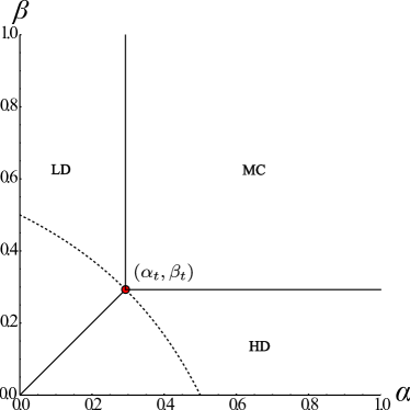
Figure 3: Typical phase diagram of TASEP-like system with three phases: HD,LD and MC. The HD-LD phase coexistence line is straight for known exactly-solvable TASEPs. The stationary state trivializes on the dashed line.

The phase coexistence lines are straight lines linking the points $(0,0)$, $(1,\beta_{t})$ and $(\alpha_{t},1)$ to the triple point $(\alpha_{t},\beta_{t})$. The values of $(\alpha_{t},\beta_{t})$ are equal to $\alpha_{t}=\beta_{t}=1/2$ in continuous time case and depend on the value of $p$ and on the update in discrete time. Also, there is a special curve in the phase diagram, corresponding to the mentioned regime with equal densities of the right and left particle reservoirs, where the stationary state trivializes, i.e. the finite segment looks as the part of translation invariant stationary infinite system. The points of this curve belong to either LD or HD phases, with the only exception, the point where the density attains its maximum equal to the density of MC phase, which is the triple point.

It is not difficult to draw the phase diagram described, given that the structure of the fixed density translation invariant stationary states of the infinite TASEP is known. Due to the choice of the Liggett-like BC the stationary state of the large system in LD (HD) phase looks like that of the left (right) reservoir at almost all the lattice except for the close vicinity of the right (left) end. It is simply the stationary state current density relation that allows one to associate every pair of $(\alpha,\beta)$ with a certain macroscopic phase at least in the case of simplest three phase scenario. This scenario is known to be realized, when the infinite system current-density relation is convex, which, as will be seen below, is also the case for gTASEP.

Note, that imposing BC in gTASEP on a finite segment is a more delicate problem than in particular cases we just described because of the additional parameter $\mu$, probability of catching up the particle ahead, controlling particle clustering in the bulk. The way how one can incorporate an analogue of this parameter into the boundary dynamics is not unique. Probably the simplest candidate, Eq. (7), was proposed in [42, 24] in an ad hoc manner consistent with the PU and BSU limits. However, no analytic predictions were made for those BC probably because it was not clear how to associate such BC with fixed density reservoirs. What allows us to partly fill this gap is the introduction of the Liggett-like boundary conditions for gTASEP.

Below we complete the following program. We first derive the Liggett-like boundary conditions, Eq. (6). To this end, we prepare the infinite stationary gTASEP starting from the system on a finite ring and calculate the probabilities of events corresponding to particle injection to and ejection from the system that is a finite part of the infinite stationary system at a given particle density. In this way, the ejection and injection probabilities are associated with the particle density values in the boundary reservoirs. In course of this derivation we also discuss calculation of averages of observables like correlation functions over the stationary state. In particular, we reproduce the known current density relation, which is then used to construct the full phase diagram as described above.

Assuming that the corresponding reservoirs govern the stationary states in LD and HD phases we obtain the explicit formulas of the triple point and of the coexistence line, which is enough to describe the full phase diagram. Remarkably, unlike the usual TASEPs studied before, the LD-HD phase coexistence line in gTASEP with Liggett-like BC is not a straight line anymore. For generic bulk dynamics it is a smooth curve connecting the origin and the triple point becoming the straight line exactly in two particular limits of TASEP with BSU and with PU. Finally, we will discuss how the phase diagram degenerates in the deterministic aggregation limit. We also present extensive numerical simulations which confirm the analytic results obtained.

IV Boundary parameters and stationary states of the infinite system

As we explained above, thermodynamic properties of LD and HD phases of gTASEP on a finite segment can be characterized in terms of those of the stationary state of the infinite system maintaining the same density as the density associated to the particle reservoirs attached to the ends of the segment. To this end, we first remind the construction of the stationary state developed in [31] and then calculate the probabilities of events, corresponding to injection and ejection probabilities to and from the boundary sites of the system. The phase diagram is constructed by juxtaposition of the current-density dependence and these probabilities.

IV.1 Stationary state of gTASEP: from a finite ring to the infinite system.

To prepare the infinite system we start from the system on a finite ring. The stationary measure was initially obtained from the mapping of gTASEP to the system with zero range interaction that admits an arbitrary number of particles in a site. At every time step $m$ particles jump to the next site from a site with $n\geq m$ with probability of the form (1), all sites being updated simultaneously. The unnormalized stationary weight of a site with $n$ particles in such a system is then given by the jumping probability normalization $f(n)$ from (4) [39]. To translate this to the TASEP language, we should replace an $n$-particle site with $n$ sites occupied by one particle each plus one empty site ahead. Though this ZRP-ASEP mapping between configurations of two models is not one to one, rather the correspondence is modulo translations, the weight $f(n)$ is then assigned to $n$-particle clusters, while the empty sites bring the unit weight.

Thus, the probability of particle configurations in gTASEP on the ring with $L$ sites and $M<L$ particles depend only on their cluster structure. Specifically, the probability of configuration

$$\bm{\mathbf{\tau}}=\left(0^{k_{1}}1^{n_{1}}\dots 0^{k_{N_{c}(\bm{\mathbf{\tau}})}}1^{n_{N_{c}(\bm{\mathbf{\tau}})}}\right)$$ (8)

with $N_{c}(\bm{\mathbf{\tau}})$ clusters of sizes $n_{1},\dots,n_{N_{c}(\bm{\mathbf{\tau}})}\geq 1$ interlaced with gaps of the lengths $k_{1},\dots,k_{N_{c}(\bm{\mathbf{\tau}})}\geq 1$ is given by

$$P_{{}_{st}}(\bm{\mathbf{\tau}}) =\frac{\delta_{k_{1}+\cdots+k_{N_{c}(\bm{\mathbf{\tau}})},L-M}\delta_{n_{1}+\dots+n_{N_{c}(\bm{\mathbf{\tau}})},M}}{\mathcal{Z}(M,L)}\prod_{l=1}^{N_{c}(\bm{\mathbf{\tau}})}f(n_{l}),$$ (9)

$$=\frac{\left(1-\nu\right)^{N_{c}(\bm{\mathbf{\tau}})}}{\mathcal{Z}(M,L)}\delta_{k_{1}+\cdots+k_{N_{c}(\bm{\mathbf{\tau}})},L-M}\delta_{n_{1}+\dots+n_{N_{c}(\bm{\mathbf{\tau}})},M}$$

where the one-cluster factor is $f(n)=(1-\nu)$ for $n\geq 1$ and $\mathcal{Z}(M,L)$ is the canonical partition function, i.e. normalization constant that ensures the unit sum of probabilities.

In the thermodynamic limit

$$M,L\to\infty,M/L=c,$$ (10)

the stationary distribution of local events depending on finitely many sites coincides with the grand-canonical distribution that assigns a fugacity $z\geq 0$ to a particle and an extra weight $f(n)=(1-\nu)$ to every cluster, so that the resulting weight of an $n$-particle cluster is

$$w_{z}(n)=z^{n}(1-\nu),$$

while an empty site is assigned the unit weight. To calculate probabilities of local events in the infinite system we start from the finite periodic system with $L$ sites, where the number of particles is not fixed, while the probability of a particle configuration (8) with the number of particles $M(\bm{\tau})=n_{1}+\dots+n_{N_{c}(\bm{\mathbf{\tau}})}$ is

$$P_{z}(\bm{\tau})=\frac{1}{\mathcal{Z}_{L}(z)}\prod_{l=1}^{N_{c}(\bm{\mathbf{\tau}})}w_{z}(n_{l})=\frac{1}{\mathcal{Z}_{L}(z)}(1-\nu)^{N_{c}(\bm{\mathbf{\tau}})}z^{M(\bm{\tau})},$$ (11)

where $\mathcal{Z}_{L}(z)$ is the partition function. Of course, in the finite system the grand-canonical distribution (38) is different from the exact canonical stationary distribution (9) of gTASEP. They become equivalent only in the thermodynamic limit (10). The grand-canonical probability can be evaluated using the transfer matrix formalism. Specifically, the probability of a particle configuration $\bm{\tau}=(\tau_{1},\dots,\tau_{L})$ with occupation numbers $\tau_{1},\dots,\tau_{L}=0,1$, is

$$P_{z}(\bm{\tau})=\frac{1}{\mathcal{Z}_{L}(z)}T_{\tau_{1},\tau_{2}}\dots T_{\tau_{L-1},\tau_{L}}T_{\tau_{L},\tau_{1}},$$

where $T_{0,0}=1$, $T_{0,1}=T_{1,0}=\sqrt{z(1-\nu)},$ and $T_{1,1}=z$. This measure is similar to the Gibbs measure of the 1D Ising model, as was first observed in [20] in the context of the TASEP with PU.

Correspondingly, for the periodic BC the partition function is given by the trace of $L$-th power of the transfer matrix

$$\mathcal{Z}_{L}(z)=\mbox{Tr}T^{L}=\lambda_{1}^{L}+\lambda_{2}^{L},$$

where $\lambda_{1},\lambda_{2}$ are the eigenvalues of the matrix $T$ defined so that $\lambda_{1}>\lambda_{2}\geq 0$

To proceed with the calculations it is convenient to introduce another variable $z_{c}$ instead of $z$, which is a unique root of equation

$$z=\frac{z_{c}\left(1-\nu z_{c}\right)}{1-z_{c}}$$

in the range

$$z_{c}\in[0,1].$$ (12)

The parameter $z_{c}$ has the meaning of particle fugacity in the associated ZRP-like model and the further equations simplify significantly written in terms of it, consisting of rational functions of $z_{c}$. In particular the eigenvalues read as follows

$$\lambda_{1} = \frac{1-\nu z_{c}}{1-z_{c}},\quad\lambda_{2}=\nu z_{c}.$$

The largest eigenvalue $\lambda_{1}$ defines the specific free energy in the thermodynamic limit (10)

$$f(z)=\lim_{L\to\infty}\frac{\ln\mathcal{Z}_{L}(z)}{L}=\ln\lambda_{1}.$$

The average density of particles is fixed by the thermodynamic relation

$$c=z\partial_{z}f(z),$$ (13)

which, written in terms of $z_{c}$ becomes

$$c=\frac{(1-\nu)z_{c}}{1-\nu\left(2-z_{c}\right)z_{c}}.$$ (14)

The density takes values in the range

$$c\in[0,1]$$ (15)

as $z_{c}$ varies in the same range.

IV.2 Correlation functions and stationary observables

To evaluate $s-$point correlation functions of the form $\left\langle\tau_{k_{1}}\dots\tau_{k_{s}}\right\rangle_{L}$, where $\left\langle a\right\rangle_{L}$ is the notation for expectation value of the random variable $a$ in the system with $L$ sites, one has to insert the matrix

$$\widehat{\tau}=\left(\begin{array}[]{cc}0&0\\ 0&1\end{array}\right)$$

into the product of transfer matrices in the places corresponding to sites $k_{1},\dots,k_{s}$:

$$\left\langle\tau_{k_{1}}\dots\tau_{k_{s}}\right\rangle_{L}=\frac{\mbox{Tr}\left[T^{k_{1}}\widehat{\tau}T^{k_{2}}\widehat{\tau}\dots\widehat{\tau}T^{L-(k_{1}+\dots+k_{s})}\right]}{\mathcal{Z}_{L}(z)}.$$ (16)

To evaluate expressions of this kind we also need the eigenvectors of $T$,

$$\mathbf{\!\!\!\!v}_{1}\!\! =\!\! \left[\begin{array}[]{c}\sqrt{\frac{\left(1-z_{c}\right)\left(1-\nu z_{c}\right)}{1-\nu\left(2-z_{c}\right)z_{c}}}\\ \\ \sqrt{\frac{z_{c}\left(1-\nu\right)}{1-\nu\left(2-z_{c}\right)z_{c}}}\end{array}\right]\!,\mathbf{v}_{2}\!=\!\left[\begin{array}[]{c}-\sqrt{\frac{z_{c}\left(1-\nu\right)}{1-\nu\left(2-z_{c}\right)z_{c}}}\\ \\ \sqrt{\frac{\left(1-z_{c}\right)\left(1-\nu z_{c}\right)}{1-\nu\left(2-z_{c}\right)z_{c}}}\end{array}\right]\!,\,\,\,\,$$ (23)

corresponding to $\lambda_{1}$ and $\lambda_{2}$ respectively, which are normalized to $\left\|v_{1}\right\|=\left\|v_{2}\right\|=1.$ In particular, one can verify the fact that the one-point correlation function indeed yields the density (14) in the thermodynamic limit

$$\left\langle\tau\right\rangle_{L}=\frac{\mbox{Tr}(\widehat{\tau}T^{L})}{\mathcal{Z}_{L}(z)}\to_{L\to\infty}(\mathbf{v}_{1},\widehat{\tau}\mathbf{v}_{1})=c.$$ (24)

Also, one can evaluate the average current as the probability of event $A$, when a particle crosses the bond connecting site $L$ with site $1$ at a time step. The particle can jump into the site that either was empty after the previous step (event $B_{0}$) or has emptied at the same step as a result of the shift of a cluster of size $k=1,2,\dots$ (event $B_{k}$). Thus, the current $j_{\infty}(c)$ maintained in the infinite system at the particle density $c$ related by (14) with $z_{c}$ can be evaluated as

$$j(c)=\mathbb{P}_{\infty}(A)=\sum_{k\geq 0}\mathbb{P_{\infty}}(A\bigcap B_{k}),$$

where the subscript in $\mathbb{P}_{\infty}$ refers to the infinite system size. The finite size $L$ lattice version of the probabilities under the sum are evaluated to

$$\mathbb{P}_{L}(A\bigcap B_{k})=p\mu^{k}\langle\tau_{L}\tau_{1}\cdots\tau_{k}(1-\tau_{k+1})\rangle_{L}$$ (25)

$$=p\mu^{k}(\langle\tau_{L}\tau_{1}\cdots\tau_{k}\rangle_{L}-\langle\tau_{L}\tau_{1}\cdots\tau_{k+1}\rangle_{L})$$

$$=p\mu^{k}z^{k}\left(\langle\tau_{1}\rangle_{L-k}\frac{\mathcal{Z}_{L-k}(z)}{\mathcal{Z}_{L}(z)}-z\langle\tau_{1}\rangle_{L-k-1}\frac{\mathcal{Z}_{L-k-1}(z)}{\mathcal{Z}_{L}(z)}\right)$$

where $\mathbb{P}_{L}$ and $\langle\cdot\rangle_{L}$ are the notations for the probability and expectation in the system of size $L$ and we used the relation

$$\langle\cdots\tau_{i}\tau_{i+1}\cdots\rangle_{L}\mathcal{Z}_{L}(z)=\langle\cdots\tau_{i}\cdots\rangle_{L-1}z\mathcal{Z}_{L-1}(z),$$

that reduces the average of a function of configuration, vanishing unless two given neighboring sites belong to the same particle cluster, to a similar average of in the system with one site excluded.

The $L\to\infty$ limit yields

$$\mathbb{P}_{\infty}(A\bigcap B_{k}) =p\mu^{k}\left(\frac{z}{\lambda_{1}}\right)^{k}c\left(1-\frac{z}{\lambda_{1}}\right)$$ (26)

$$=p\mu^{k}cz_{c}^{k}(1-z_{c}),\quad k=0,1,\cdots.$$

Then, for the current we have

$$j(c) =pc(1-z_{c})\sum_{k\geq 0}(\mu z_{c})^{k}$$ (27)

$$=\frac{\left(1-z_{c}\right)z_{c}(\mu-\nu)}{\left(1-\mu z_{c}\right)\left(\nu z_{c}^{2}-2\nu z_{c}+1\right)},$$ (28)

which is the expression previously obtained in [27, 31]. For all $0\leq\mu\leq 1$ and $0<p\leq 1$ it is a concave function of the density taking values $j(0)=j(1)=0$ at $c=0$ and $c=1$ respectively, and hence having a single maximum in (15), see fig. 4.

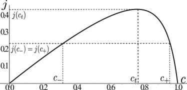
Figure 4: An example of current density plot for $p=0.8,\mu=0.9.$ The points $c_{+},c_{-}$ and $c_{t}$ show a pair of left and right reservoir densities corresponding to a point at the phase coexistence line and the density of MC phase respectively.

IV.3 Injection and ejection probabilities

Let us evaluate the values of probabilities for a particle to enter and exit the system in gTASEP on a segment with open ends, implying that they are the same as the probability of similar moves in the infinite system in translation invariant steady state at fugacity $z_{c}$ (and hence at density (14)). For particles entering the system we can define the family of probabilities

$$\alpha_{k}=\mathbb{P_{\infty}}(A|B_{k})=\frac{\mathbb{P_{\infty}}(A\bigcap B_{k})}{\mathbb{P}_{\infty}(B_{k})},\quad k=0,1,\dots$$

where $\alpha_{0}$ is the probability for a particle to enter a site conditioned on the fact that this site remained empty after the previous step, while $\alpha_{k}$ with $k>0$ is a similar probability conditioned on the fact that the site has emptied after the one-step shift of a cluster of $k>0$ particles at the same time step. While the numerators were obtained in (25,26) the denominators can be evaluated similarly

$$\mathbb{P}_{L}(B_{0}) =\langle(1-\tau_{1})\rangle_{L},$$

$$\mathbb{P}_{L}(B_{k}) =p\mu^{k-1}\langle\tau_{1}\cdots\tau_{k}(1-\tau_{k+1})\rangle_{L},\quad k\geq 1.$$

In the $L\to\infty$ limit this yields

$$\mathbb{P}_{\infty}(B_{0}) =1-c$$

$$\mathbb{P}_{\infty}(B_{k}) =p\mu^{k-1}cz_{c}^{k-1}(1-z_{c}).$$

Thus we have

$$\alpha_{0}=\frac{pc(1-z_{c})}{1-c}=\frac{(\mu-\nu)z_{c}}{(1-\nu z_{c})}$$ (29)

and

$$\alpha_{k}=\mu z_{c},\quad k\geq 1.$$ (30)

One can see that $\alpha_{k}$ does not depend on $k$, when $k\geq 1$. Thus, similarly to the bulk dynamics it is enough to define two entrance probabilities

$$\alpha =\frac{(\mu-\nu)z_{c}}{(1-\nu z_{c})},$$ (31)

$$\tilde{\alpha} =\mu z_{c},$$ (32)

for the particle to enter the first site that was empty after the previous step and that has emptied at the current step respectively. They are parametrically related via the mutual dependence on the parameter $z_{c}$. When $z_{c}$ varies in the range (12) that corresponds to the densities in (15), $\alpha$ and $\tilde{\alpha}$ take values in

$$\alpha \in[0,p],\quad\tilde{\alpha}\in[0,\mu],$$ (33)

being monotonous functions of $z_{c}.$ Eliminating $z_{c}$ between (31) and (32), we obtain (6).

Similarly, to evaluate the analogue of probability $\beta$ for the particle to leave the system from the last site we should find the probability for the particle to jump out of the site conditioned on the presence of a particle at this site, which reads

$$\beta =\mathbb{P}(A|\{\tau_{L}=1\})$$

$$=\frac{j(c)}{c}=\frac{(1-z_{c})(\mu-\nu)}{(1-\nu)(1-\mu z_{c})}.$$ (34)

It also takes values in the range

$$\beta\in[0,p]$$ (35)

for $z_{c}$ in (12). Both $\alpha$ and $\beta$ are monotonous functions of $z_{c}$ (increasing and decreasing respectively) and hence of the density.

V Phase diagram of gTASEP

Let us use relations (14,27,31-34) to establish the form of the phase diagram of gTASEP on a segment. The mechanism of the stationary state selection in the driven diffusive systems with the current with a unique maximum in the current-density plot was described in [5, 45] using purely hydrodynamic arguments. Below we apply their findings to construct the phase diagram of gTASEP.

V.1 Stationary state trivialization curve

First we note that when the values of $\alpha$ and $\beta$ satisfy (33,35) the densities $c_{-}$and $c_{+}$ of the left and right reservoirs associated with our BC are obtained by eliminating $z_{c}$ between the $\alpha$ and $c$, eqs.(14,31), and $\beta$ and and $c$, eqs. (14,34), which yields

$$c_{-} =\frac{\alpha^{2}(\mu-p)+\alpha p(1-\mu)}{\alpha^{2}(\mu-p)+p^{2}(1-\mu)}$$ (36)

and

$$c_{+}=\frac{(p-\beta)(p-\beta\mu)}{p\left(p-\beta^{2}\right)+\beta\mu(\beta+(\beta-2)p)},$$ (37)

respectively. A special curve in the phase diagram, at which the densities of the left and right reservoirs are the same, $c_{+}=c_{-}$, can be obtained by eliminating $z_{c}$ between (34) and (31), which yields

$$(1-\beta)(1-\alpha)=1-p.$$ (38)

At this curve the system on the segment looks like a part of the infinite system in the translation invariant steady state. In this case, the exact stationary measure similar to that of 1D Ising model can be obtained as $L$-site correlation function at the infinite lattice and expressed in terms of a product of $2\times 2$ matrices, sandwiched between two vectors $\boldsymbol{v}_{1}$ from (23). In particular, the macroscopic density profile is perfectly flat with $c=c_{+}=c_{-}$ and the current is $j(c)$. The relation (38) was already obtained before for the cases of parallel and backward sequential updates, where it defines the regime in which the representation of the algebra used to construct the matrix product stationary state trivializes. Remarkably, this relation is preserved at the arbitrary values of $\mu$.

V.2 Triple point

As we move along the curve (38) from $(\alpha,\beta)=(0,p)$ to $(\alpha,\beta)=(p,0)$ the density $c=c_{-}=c_{+}$ continuously grows from $c=0$ to $c=1$ as well as the associated fugacity $z_{c}$. At the same time, the particle current $j(c)$ grows from $j(0)=0$ to its unique maximum $j_{\max}=j(c_{t})$ attained at the density $c=c_{t}$, the unique root of the equation

$$\frac{dj(c)}{dc}=0,$$

in the density range (15), and then decreases back to $j(1)=0$. The point corresponding to $c=c_{t}$ is a triple point. Since the current attains its maximal value at $c_{t}$ and this value is the largest that the bulk can sustain, a further increase neither of $\alpha$ nor of $\beta$ causes an increase of the current. Thus, the rectangle $(\alpha,\beta)\in[\alpha_{t},1]\times[\beta_{t},1])$ is the maximal current phase. Remarkably, as follows from (38) its area does not depend on the value of $\mu$.

The value of $c_{t}$ as well as $j_{\max}$,$\alpha_{t},\tilde{\alpha}_{t}$ and $\beta_{t}$ can be obtained by evaluating formulas (14,27,31,32,34) respectively at $z_{c}$ given by a unique root of the polynomial

$$P_{\mathrm{T}}(z)=\mu\nu(z^{4}-2z^{3}+2z^{2})-(\mu+\nu)z^{2}+2z-1$$ (39)

in the range (12), see Figs. 5,6. In two cases $\mu=0$ and $\nu=0$ ($\mu=p$) corresponding to PU and BSU respectively $P_{\mathrm{T}}(z)$ simplifies to the quadratic polynomial, and the explicit values of $c,j_{\infty}$ and $\alpha_{t},\tilde{\alpha}_{t}$ and $\beta_{t}$ at the triple point can easily be evaluated reproducing the known expressions obtained before. In particular

$$\alpha_{t}=\beta_{t}=1-\sqrt{1-p}$$ (40)

in both cases. Remarkably, these are the only two cases, when $\alpha_{t}$ coincides with $\beta_{t}$. Furthermore, as follows from (40), given $p$, the values of $\alpha_{t}$ and $\beta_{t}$ are not monotonous as functions of $\mu$ in the interval $\mu\in[0,p]$. As $\mu$ increases, the value of $\alpha_{t}$ ($\beta_{t}$) starting from (40) at $\mu=0$ first increases (decreases), but then turns back to (40) at $\mu=p$ and continues to decrease (increase) up to $\alpha_{t}=0$, ($\beta_{t}=p$) at $\mu=1$.

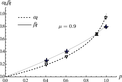
Figure 5: The values of $\alpha_{t}$ and $\beta_{t}$ at the triple point as functions of $p$ corresponding to $\mu=0.9$. The graphs cross at two points corresponding to PU and BSU cases. The down- and up-triangles, $\triangledown,\triangle,$ are their values measured in simulations. The cross symbols, ${+}$, are the values of $\beta_{t}$ in gTASEP with left BC (7), which coincide with ones with Liggett’s BC within the numerical precision.

Figure 6: The values of $\alpha_{t}$ and $\beta_{t}$ at the triple point as functions of $\mu$ corresponding to $p=0.6$ and $p=0.9$. The graphs cross at two points corresponding to to PU and BSU cases. The down- and up-triangles, $\triangledown,\triangle,$ are their values measured in simulations. The cross symbols, $+$, are the values of $\beta_{t}$ in gTASEP with left BC (7), which coincide with ones with Liggett’s BC within the numerical precision.

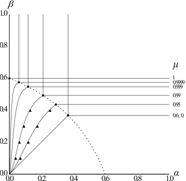
(a)

(b)

Figure 7: The phase diagrams of gTASEP in $\alpha-\beta$ plane for (a) $p=0.6$ and (b) $p=0.9$ with various values of $\mu$. The dashed curves are the lines (38), where the stationary state trivializes. The triangle symbols, $\blacktriangle$, are the simulation results.

V.3 HD-LD phase coexistence line

Let us finally describe the HD and LD phases and, in particular, the phase coexistence line between them. The LD (HD) phase is established, when $j(c_{-})<\min(j(c_{+}),j_{\max})$ $(j(c_{+})<\min(j(c_{-}),j_{\max})$. It includes the points of the phase diagram under the curve (38), where the boundaries are associated with reservoirs at densities $c_{-}$ and $c_{+}$, as well as for larger values of $\beta$ ($\alpha$). The particle density is equal to $c_{-}(c_{+})$ in almost all the system, up to a close vicinity of the right (left) segment end, where the density profile bends to reach the density of the left (right) reservoir.

The phase coexistence line connects the origin $(\alpha,\beta)=(0,0)$ to the triple point $(\alpha_{t},\beta_{t})$ and can be obtained as a set of pairs $(\alpha,\beta)$ associated with densities $(c_{-},c_{+})$ solving equation

$$j(c_{-})=j(c_{+}),$$ (41)

see Fig. 7.

In terms of fugacities $z_{-},z_{+}$ associated with densities $c_{-},c_{+}$ this equation is reduced to finding the 1D subset of $(z_{-},z_{+})\in[0,z_{t}]\times[z_{t},1]$, where polynomial

$$P_{\mathrm{C}}(z_{-},z_{+}) =\mu\nu z_{+}^{2}z_{-}^{2}-\mu\nu z_{+}z_{-}^{2}-\mu\nu z_{+}^{2}z_{-}$$

$$-z_{+}z_{-}(\mu+\nu-2\mu\nu)+z_{-}+z_{+}-1$$

vanishes, which amounts to solving the quadratic equation, say for $z_{+}$ in terms of $z_{-}$. Substituting solutions obtained for $(z_{-},z_{+})$ into (31,34) respectively we obtain the required parametric curve in $(\alpha,\beta)$ coordinates as functions of $z_{-}$ varying in the range $0\leq z_{-}\leq z_{t}$. The result simplifies significantly in the PU and BSU cases $\mu=0$ and $\nu=0$ respectively, yielding the known result, the straight line segment $\alpha=\beta\in[0,1-\sqrt{1-p}].$

As one can see in fig. 7, the shape of the phase coexistence line starting from the straight segment at $\mu=0$ is bending as $\mu$ increases, first rotating clockwise, so that the area of LD phase grows, then rotating anticlockwise to return back to the same straight segment at $\mu=p$. Then, it is again bending and moving towards the $\beta$-axis, so that the low density phase disappears in the limit $\mu\to 1$.

V.4 Deterministic aggregation limit

The limit $\mu\to 1$ at fixed $0<p<1$ is associated with deterministic aggregation regime in [31], in which particles tend to gather in large clusters. With Liggett-like BC we automatically have $\tilde{\alpha}\to 1$ in this limit for any $0<\alpha<1$, so that in the stationary state all the lattice is occupied by a single cluster that sometimes (with probability $\beta$) shifts as a whole one step forward with immediate filling the emptied left-most site, so that the density maintained is exactly $c=1$. To see the lower densities one should consider the joint limits $\mu\to 1$ and $z_{\pm}\to 1$ corresponding to $\alpha\to 0$ and $\beta\to p$ in LD and HD phases respectively.

Specifically, following [32] one can consider the family of scalings parameterized by an exponent $\mathfrak{b}\in(0,1)$ setting

$$z_{c}=1-\zeta(1-\mu)^{\mathfrak{b}},$$ (42)

where $\zeta>0$ is a scaling variable. Under this scaling we have

$$c = \left\{\begin{matrix}(1-\mu)^{1-2\mathfrak{b}}\left(\zeta^{2}(1-p)\right)^{-1}&\mathfrak{b}<1/2\\ (1+\zeta^{2}(1-p))^{-1}&\mathfrak{b}=1/2\\ 1-(1-p)\zeta^{2}(1-\mu)^{2\mathfrak{b}-1},&\mathfrak{b}>1/2\end{matrix}\right.$$

$$+\,O\left((1-\mu)^{2|2\mathfrak{b}-1|},(1-\mu)^{(|2\mathfrak{b}-1|+1)/2}\right),$$

i.e., $\mathfrak{b}=1/2$ corresponds to the density ranging in $c\in(0,1)$ as $\zeta\in(0,\infty)$ with values away from $c=0$ and $c=1$, while $\mathfrak{b}<1/2$ and $\mathfrak{b}>1/2$ are responsible for the close vicinities of the extreme density values respectively.

Corresponding entrance and exit probabilities will than scale as

$$\alpha = \frac{p(1-\mu)^{1-\mathfrak{b}}}{\zeta(1-p)}+O\left((1-\mu),(1-\mu)^{2(1-\mathfrak{b})}\right),$$ (44)

$$\tilde{\alpha} = \left(1-\zeta(1-\mu)^{1-\mathfrak{b}}\right)+O\left((1-\mu)\right),$$ (45)

$$\beta = p\left(1-\zeta^{-1}(1-\mu)^{1-\mathfrak{b}}\right)$$

$$\,\,\,\,\,\,\,\,\,\,\,\,\,\,\,\,\,\,\,\,\,\,\,\,\,\,\,\,\,\,\,\,+\,O\left((1-\mu),(1-\mu)^{2(1-\mathfrak{b})}\right).$$

in LD and HD phases respectively. The formulas (44,45) and (V.4) are the entrance and exit probabilities that maintain the densities (V.4) in LD and HD phases as $\mu\to 1$, provided that $\alpha$ and $\beta$ are less than $\alpha_{t}$ and $\beta_{t}$ respectively.

To characterize the triple point we study the roots of $P_{\mathrm{T}}(z)$, (39), in the limit $\mu\to 1$. When $\mu=1$, this polynomial has a triple root $z=1$. Then, examining the expansion of these roots in powers of $(1-\mu)$ we find the fugacity $z_{c}$ given by a single real root located in the range (12) to be

$$z_{c}=1-\frac{(1-\mu)^{2/3}}{(2(1-p))^{1/3}}+O(1-\mu).$$ (47)

Respectively, the triple point density and entrance and exit probabilities are given by formulas (V.4-V.4) with $\mathfrak{b}=2/3$ and $\zeta=(2(1-p))^{-1/3}+O(1-\mu)^{1/3}.$

Finally, we note that the crossover between the KPZ and deterministic aggregation regimes studied in [31, 32] corresponded to such a space scale, in which one typically observes finitely many huge particle clusters. This fact suggested a specific scaling of either the system size, when the stationary state on the ring was studied, or spacial units, for the non-stationary gTASEP in the infinite system. In our case, we also expect that the change of the scaling behavior of the particle current fluctuations will be observed in a joint limit $\mu\to 1$ and $L\to\infty$, such that the mean length per particle cluster $c^{-1}\langle l_{\mathrm{cl}}\rangle$ is comparable with the system size $L$. Here

$$\left\langle l_{cl}\right\rangle=(1-z_{c})^{-1}\simeq\sqrt{c/[(1-c)(1-\mu)]}$$

is the mean stationary cluster size at the density $c$. Hence, we conjecture that the crossover will be governed by the scaling variable

$$\tau=L(1-\mu)^{|\mathfrak{b}-\frac{1}{2}|+\frac{1}{2}}$$ (48)

that stays finite in the limit under consideration, in the same way as it was in [31, 32], where the system crossed over from KPZ to fully correlated Gaussian motion of particles within a single giant cluster. In particular, we expect that in the vicinity of the triple point the current large deviation function will cross over from the form obtained in [46] to the pure Gaussian one as $\tau$ varies in the range $\tau\in[0,\infty)$.

VI Simulation results

To verify some of the analytical findings, we also executed an independent numerical study of the steady state properties of the gTASEP, equipped with Liggett’s BC, defined by probabilities $\alpha,\beta$ and additional probability $\tilde{\alpha}$ given by formula (6). We performed numerical simulations of the system with the following parameters. A system of $L=200$ sites was studied. $N_{\tau}=800000$ time steps were omitted to ensure that the system has reached stationary state. The length of the time sequences we used for recording the physical quantities (e.g., density distribution along the system length $c(x)$, $x\in(0,1]$ bulk density $c_{b}$, particle current $j$, etc.) was $N_{t}=2^{21}$ , and averaging of over $N_{\text{ens}}=100$ independent simulation runs of the system was performed.

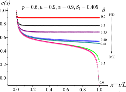
(a)

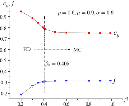
(b)

Figure 8: Manifestation of HD-MC transitions. Numerical results for different values of $\beta$ at fixed $p=0.6,\mu=0.9,\alpha=0.9>\alpha_{t}=0.3228$: (a) density profiles $c(x),x\in(0,1]$ along the system; (b) dependence of the current $j$ and the bulk density $c_{b}$ on $\beta$ at fixed $\alpha,p,\mu$.

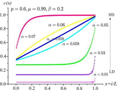
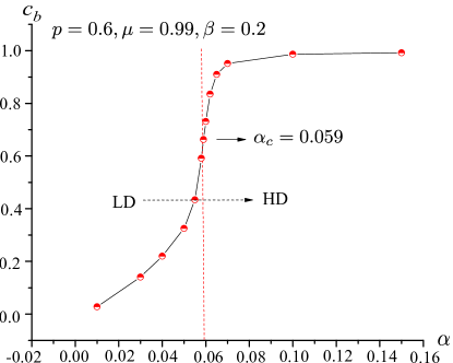
(a) (b)

Figure 9: Manifestation of HD-LD transitions. Numerical results for different values of $\alpha\in(0.01,0.07)$ at fixed $p=0.6,\mu=0.99,\beta=0.2<\beta_{t}=0.49296$. (a) Density profiles for different values of $\alpha$. The profile at the coexistence line is perfectly straight. The change of the density profiles shape is used to determine the coexistence line coordinates. (b) Change of the bulk density $c_{b}$ at fixed $\beta$ as $\alpha$ crosses its value $\alpha_{c}$ at the HD-LD coexistence line. The transition is a bit “smoothed” since the system is finite.

In Fig. 8 we show the density profiles $c(x),x\in[0,1]$, obtained from the simulations in various regimes. In LD (HD) phase they are typically flat in the whole system except for a close vicinity of the right (left) end, where the profile bends to reach the density of the corresponding reservoir. This confirms the fact that the stationary state of gTASEP in LD (HD) phase in a finite segment is close to that of the infinite system almost in the whole system. In MC phase the profile maintains the MC density in the bulk and bends close to both ends of the segment to reach the densities of the reservoirs. As usual, the $L$-dependent size of the domain, where the density deviates from its bulk value, is much larger in MC phase than in HD and LD phases, resulting in the S-shaped profile in the finite system. In Fig. 8(a) the density profiles at fixed $p,\mu$ and $\alpha>\alpha_{t}$ are shown for seven values of $\beta$. As one can see, for low values of $\beta$ one has almost constant density profiles bending near the left end and after reaching the triple point $\beta_{t}$ the profiles gradually transform to the MC $S$-like shape.

In order to determine the triple point values $\alpha_{t}$ and $\beta_{t}$ for any given pair of values of the parameters $p,\mu$ we used the dependence of the current $j$ on $\alpha$ (respectively, on $\beta$) at fixed $\beta$ (respectively, fixed $\alpha$), similarly to that in [47]. To illustrate that, in Fig. 8(b) we present simulation results for the dependence of the current $j$ and the bulk density $c_{b}$ on $\beta$ at fixed $\alpha,p,\mu$. On the left side of the vertical dashed line the system is in HD phase (characterized by high values of $c_{b}$ and low values of $j$). After the transition point at $\beta_{t}$ (on the right side of the vertical dashed line) the dependence of the current $j$ on $\beta$ (and $c_{b}$) reaches a plateau, signaling that the system is in the MC phase.

We obtained the values of $\alpha_{t}$ and $\beta_{t}$ at fixed $p=0.9$ and $p=0.6$ for different values of $\mu$, Fig. 6, and at fixed $\mu=0.9$ for several values of $p$, Fig. 5. As can be seen from figures, the numerical values of $\alpha_{t}$ and $\beta_{t}$ determined with precision $\pm 0.005$ corroborate with high accuracy the obtained analytical results.

If we fix the values of $\alpha_{t}$ ($\beta_{t}$) below the one at the triple point and vary $\beta_{t}$ ($\alpha_{t}$) in its range, we will observe the bulk density jump that corresponds to the LD-HD first order phase transition. In Fig. 9(a) we show the profiles at fixed $p,\mu$ and $\beta<\beta_{t}$ at seven different values. One can see that almost constant density profiles bending at the right end at small $\alpha$ transforms to those bending at the left end at large $\alpha$ through the point, where the density profile is an exact straight line connecting the densities of the reservoirs. This is the point at the coexistence line. We used this fact to locate points of the coexistence line in simulations data. Also the bulk density $c_{b}$ that is expected to make a sharp jump from LD to HD density value at this point, see Fig. 9(b). One can see in Fig. 7 that the points at the coexistence line obtained from the simulations are in excellent agreement with the analytically predicted curves.

Finally, it is interesting to compare the phase diagrams obtained for gTASEP with Liggett-like BC with those for the previously studied model with with BC (7), see Fig. 10. First, we note that the unlike the phase diagram of gTASEP with Liggett-like BC, the LD-HD phase coexistence line obtained with BC (7) is a straight line. Since we do not have an analytic theory of gTASEP with BC (7) we do not know the reason for this behavior.

Also we note that since the HD and MC phases are governed by the right reservoir and the bulk respectively the value of $\beta_{t}$ does not depend on the rules of update of the left end and thus is the same for the two types of BC. Indeed, as can be seen in Figs. 5,6, the values of $\beta_{t}$ measure with the two different BC coincide within the numerical precision. On the other hand, as explained in the end of section II, BC (7) enhance the effective flow into the system when $\alpha<p$ and suppress it when $\alpha>p$ in the repulsive regime, $p>\mu$, and vice versa in the attractive regime, $p<\mu$. Therefore the value of $\alpha_{t}$ is greater (less) for BC (7) than for Liggett-like BC, when $p>\mu$ ($\mu>p$). This in turn means that the area of MC phase is greater for BC (7) than for Liggett-like BC in the repulsive regime and vice versa in the attractive one.

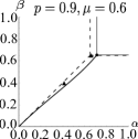
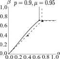
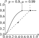
Figure 10: Comparison of the phase diagrams of gTASEP with Liggett-like BC (solid lines) and those with BC (7) (dashed lines) at three different values of $p,\mu$. Black triangles $\blacktriangle$ are the simulations results. We show the triple point and yet another point illustrating that the HD-LD phase coexistence line of in gTASEP with BC (7) is straight. One can see that the triple point of gTASEP with BC (7) is to the left from that with Liggett-like BC when $p>\mu$ and is to the right, when $\mu>p$.

VII Conclusion and discussion

To conclude, we proposed new boundary conditions for the TASEP with generalized update on an open segment. They mimic the infinite reservoirs in translation invariant steady states attached to the segment ends. With these boundary conditions the phase diagram can be constructed explicitly. We confirmed our analytic predictions by extensive numerical simulations and compared them with the previous results on the same model with boundary conditions defined in different way. Of course, the most interesting part of the research subject is far beyond the phase diagram. In particular, this would be the fluctuation statistics of particle density and current and especially the universal limit laws describing the large scale behavior of the system. For this, we need an exact solution at least for the steady state, for which the matrix product is known to be the main tool. At the moment the trivial $2\times 2$ matrix product stationary state exists only at the special line of the phase diagram, where the segment looks as a part of the infinite translation invariant stationary system. Also, the matrix product solution is available for two particular limits of the generalized model we consider. This makes us expect that a generalized matrix algebra that provides the matrix product stationary state of our system can also be obtained, and the proposed boundary conditions are the first candidate for obtaining its tractable representation. Then, our results would serve as the initial test of the exact solution. This is the next step for further investigation. We have also speculated about the crossover between the KPZ regime and the deterministic aggregation limit and conjectured the form of the scaling parameter controlling the transition. The scaling functions describing the crossover could also be studied starting from the exact solution. This would provide us with an example of breaking up the KPZ universality in the open system, when the interaction causes an unbounded growth of spatial correlation length.