Ultraclean Andreev interferometers

Abstract

Coupling a two-terminal Josephson junction to the stationary modes of the electromagnetic field produces the so-called Fiske resonances. Here, we propose another mechanism based on the exchange between the static Andreev bound states (ABS) and a nonequilibrium Fermi surface in an ultraclean multiterminal device. As a simple model, we consider an effective $S_{a}$-$N_{eff}$-$S_{b}$ double junction connecting the superconductors $S_{a}$ and $S_{b}$ to the infinite central normal metal $N_{eff}$. We find that the underlying microscopic process of phase-sensitive Andreev reflection (phase-AR) produces the possibility of an inversion, that is, the conductance can be larger at half-flux quantum than in zero field. The inversion-noninversion alternate as the bias voltage is increased. In addition, if the central region $N_{eff}$ is an integrable billiard connected to an infinite normal reservoir, we find that the standard ABS are replaced by one- and two-particle Andreev resonances that can be probed by the bias voltage. Finally, we find that, in the corresponding all-superconducting Andreev interferometer, the superconducting gap produces protection against the short relaxation time of the quasiparticle continua if the time-periodic dynamics is treated as a perturbation. The spectrum of the two-particle resonances is then sparse inside the spectrum of the pairs of one-particle resonances. Our work supports the nonFloquet intrinsic resonances in two-dimensional metal-based Andreev interferometers, and challenges the Floquet theory of multiterminal Josephson junctions.

I Introduction

In the continuation of Anderson’s theory of gauge invariance in superconductors Anderson1 ; Anderson2 , Josephson demonstrated Josephson that a dissipationless DC-supercurrent $I(\varphi_{b}-\varphi_{a})=I_{c}\sin(\varphi_{b}-\varphi_{a})$ flows through a two-terminal weak link bridging the right and left superconductors $S_{b}$ and $S_{a}$. The difference $\varphi_{b}-\varphi_{a}$ is between their macroscopic superconducting phase variables $\varphi_{b}$ and $\varphi_{a}$.

More recently, it came as a surprise Freyn2011 that transient multiplets of Cooper pairs, also known as the Cooper quartets, sextets, octets, and so on, could be revealed in the DC-current, at equilibrium or in a device biased at the commensurate voltage differences. In the voltage-biased three-terminal devices, the third terminal is qualitatively analogous Cuevas-Pothier to the RF source in the two-terminal Shapiro step experiments Shapiro . The theory of the quartets Freyn2011 ; Cuevas-Pothier ; Melin2016 ; Melin2017 ; Melin2019 ; Doucot2020 ; Melin2020 ; Melin2020a ; Melin2021 ; Melin2022 ; Melin2023 ; Melin2023a ; Melin-Winkelmann-Danneau is in agreement with a series of experiments realized in the Grenoble Pfeffer2014 , the Weizmann Institute Cohen2018 and the Harvard Huang2022 groups. Classical synchronization in the multiterminal resistively shunted junction (RSJ) model is also compatible with some of the DC-current experimental data on graphene-based multiterminal Josephson junctions Finkelstein1 ; Finkelstein2 ; Finkelstein3 ; Zhang1 ; Gupta2023 ; Graziano2020 . However, the adiabatic dynamics of the standard RSJ model cannot explain the zero-frequency quantum noise cross-correlation experiment of the Weizmann group Cohen2018 . As shown in Ref. Freyn2011, , the three-body quartet phase is also operational at equilibrium, see the recent experiment from the Zürich group collaborationZurich . The Minnesota group Pribiag reported nonconvex critical current contours Pankratova2020 ; Melin2023a in three-terminal Josephson junctions, as a further signature Melin2023a of the three-body quartet phase combination. In addition, many other effects topo1 ; topo2 ; topo3 ; topo4 ; molecule1 ; molecule2 ; molecule3 ; molecule4 ; Gupta2023 ; Zhang2023 ; Matsuo2022 ; Pankratova2020 ; Graziano2020 ; Khan2021 ; Finkelstein1 have focused interest in the field of multiterminal Josephson junctions, such as the production of Weyl-point singularities and topologically quantized transconductance topo1 ; topo2 ; topo3 ; topo4 , the emergence of avoided crossings in the spectra of Andreev bound states molecule1 ; molecule2 ; molecule3 ; molecule4 , the multiterminal Josephson diode effect Gupta2023 ; Zhang2023 ; Finkelstein1 , and so on.

Coming back to the quartets, the recent Harvard group experiment Huang2022 revealed the so-called inversion in a device consisting of a grounded superconducting loop ending at the contacts $S_{c,1}$ and $S_{c,2}$, and pierced by the magnetic flux $\Phi$. A four-terminal junction is formed with two other proximate superconducting contacts $S_{a}$ and $S_{b}$ biased at the voltages $V_{a,b}=\pm V$, respectively. As it is mentioned above, this experiment Huang2022 reported the inversion, that is, the quartet anomaly can be stronger at the flux $\Phi=\pi$ than in zero magnetic field $\Phi=0$. The noninversion-inversion cross-over can also be monitored by the bias voltage on the quartet line. At first glance, this experimental result Huang2022 seems to contradict constructive or destructive interference under magnetic field. Several models have been investigated as candidates to capture the inversion: the split quartets emerging from higher-order perturbation theory in the tunneling amplitudes Melin2020 , the Floquet theory in a zero-dimensional (0D) quantum dot Melin2020a , and the non-Hermitian effects related to the emergence of exceptional point singularities in a four-terminal two-node circuit model Melin2022 .

However, very recently, the Penn State group demonstrated a sequence of inversion-noninversion alternations as a function of the bias voltage $V_{B}$ in a $(S_{a},\,S_{b},\,S_{B})$ three-terminal Josephson junction connecting a grounded loop terminated at $S_{a}$ and $S_{b}$ to the third superconducting lead $S_{B}$ at the bottom. This three-terminal Josephson junction biased at $(0,\,0,\,V_{B})$ forms an effective all-superconducting Andreev interferometer controlled by the magnetic flux $\Phi$ and the voltage $V_{B}$. Concerning nanofabrication, the Penn State group experiment is realized with superconducting leads that are edge-connected to an encapsulated graphene monolayer gated far from the Dirac point. Given those experimental conditions, the fully ballistic description of the ultraclean limit seems to be an appropriate starting point.

Our analysis of a $(S_{a},\,S_{b},\,S_{B})$ all-superconducting Andreev interferometer biased at $(0,\,0,\,V_{B})$ is guided by the observation that the difference $\varphi_{b}-\varphi_{a}$ between the macroscopic phase variables $\varphi_{b}$ and $\varphi_{a}$ of the superconductors $S_{b}$ and $S_{a}$ is the only static combination $\varphi_{b}-\varphi_{a}\simeq\Phi$, where $\Phi$ is the flux enclosed in the loop. For instance, the two-body phase differences $\varphi_{a}-\varphi_{B}$, $\varphi_{b}-\varphi_{B}$ or the three-body Cooper quartet phase combinations, such as $\varphi_{q}=\varphi_{a}+\varphi_{b}-2\varphi_{B}$, are AC if the voltage biasing is at $(0,\,0,\,V_{B})$. It is concluded that the DC-current response of an all-superconducting Andreev interferometer biased at the voltages $(0,\,0,\,V_{B})$ solely operates in the Andreev reflection channel instead of the Josephson channel for the quartets in the four-terminal Harvard group experiment Huang2022 .

The goal of the present paper is to propose a simplified model for this type of ultraclean $(S_{a},\,S_{b},\,S_{B})$ all-superconducting Andreev interferometer biased at $(0,\,0,\,V_{B})$. Given the absence of DC-transport of Cooper pairs in the direct Josephson channel from $S_{B}$ to $(S_{a},\,S_{b})$, we qualitatively replace the bottom superconducting lead $S_{B}$ by the normal lead $N_{B}$, postponing for the end of the paper the discussion of the initial all-superconducting Andreev interferometer. The considered $(S_{a},\,S_{b},\,N_{B})$ normal-superconducting Andreev interferometer is schematically shown in Fig. 1a.

The spectrum of ballistic two-terminal Josephson junctions was calculated in Refs. Kulik, ; Ishii, ; Bagwell, . Using semiclassical quantization, Kulik Kulik addressed perfectly transparent contacts connecting a rectangular normal metal $N$ to the right and left superconductors $S_{b}$ and $S_{a}$ sustaining the superconducting phase variables $\varphi_{b}$ and $\varphi_{a}$, respectively. Then, each ABS is characterized by an independent quantum number and some of the ABS are free to cross each other at the superconducting phase differences $\varphi_{b}-\varphi_{a}=0$ or $\varphi_{b}-\varphi_{a}=\pi$. BagwellBagwell addressed backscattering by an impurity located in the normal metal $N$ and found avoided energy level crossings due to the formation of blocks in the Bogoliubov-de Gennes Hamiltonian, between states at the opposite wave-vectors.

A relevant question is the following: what is the effect of attaching the bottom normal lead $N_{B}$ biased at the voltage $V_{B}$, according to Fig. 1a?

An answer is the following: It was demonstrated by Parcollet and Hooley Parcollet-Hooley that, in the 0D limit, the $V_{B}$-sensitive distribution function of the central conductor ensures current conservation. The effect appears at zero order in the tunneling amplitude between the 0D quantum dot and the leads Parcollet-Hooley . As a point of comparison, the quartet Rabi resonances were already addressed in three-terminal Josephson junctions biased at the voltages $(V,\,-V,\,0)$, see Ref. Melin2017, . It was then demonstrated that tiny relaxation produces a continuum of states, resulting in a Fermi surface on the central 0D quantum dot, and in the appearance of low energy or long time scales. Those low-energy scales physically encode the line-width broadening of the Floquet resonances, which is exponentially small in the inverse of the voltage at small relaxation. This point of view of the Floquet theory was successfully developed in a subsequent series of papers Melin2020a ; Melin2019 ; Doucot2020 ; Melin2021 ; Melin2022 .

Now, we come back to modeling a two-dimensional (2D) metal connecting the two grounded left and right superconducting leads $S_{a}$ and $S_{b}$ and the bottom normal lead $N_{B}$ biased at the voltage $V_{B}$. We intuitively envision the Bagwell Bagwell or Bagwell-like spectra plotted as a function of the superconducting phase difference $\varphi_{b}-\varphi_{a}$, and introduce the central region effective Fermi energy $\mu_{N}(V_{B})$, which is monitored by the voltage $V_{B}$. In general, the Andreev current depends on the 2D metal populations which should be calculated self-consistently in the elastic regime, in such a way as to fulfill the condition of current conservation. Then, each of the limiting quantum transport regimes of sequential tunneling and elastic cotunneling can qualitatively be described by the Bagwell-like spectra evaluated at the effective Fermi energy $\mu_{N}(V_{B})$:

(i) We find resonances if the Bagwell-like energy level $E_{p}(\varphi_{b}-\varphi_{a})$ crosses the nonequilibrium effective Fermi surface, i.e. if the condition $E_{p}(\varphi_{b}-\varphi_{a})=\mu_{N}(V_{B})$ is fulfilled.

(ii) The corresponding superconducting phase difference oscillates between $\varphi_{b}-\varphi_{a}=\pi$ and $\varphi_{b}-\varphi_{a}=0$, thus producing alternations between $dI_{B}/dV_{B}$ that resonates at $\varphi_{b}-\varphi_{a}=\pi$ (inversion) or at $\varphi_{b}-\varphi_{a}=0$ (noninversion) as the bias voltage $V_{B}$ is increased.

To summarize, those simple physical arguments yield multiple alternations between inversion and noninversion, and the emergence of the intrinsic resonances. The goal of this paper is to demonstrate that the microscopic theory offers a kind of “unified” computational point of view on both of these phenomena. Our results will be summarized as follows: (i) The calculation of the conductance of a normal-superconducting Andreev interferometer reveals undamped oscillations as a function of the bias voltage, while their diffusive-limit counterpart Wilhelm ; Nakano ; Zaitsev ; Kadigrobov ; Volkov ; Nazarov1 ; Nazarov2 ; Yip ; Belzig ; Zaikin1 ; Zaikin2 ; Zaikin3 ; Zaikin4 feature both oscillations and damping controlled by the Thouless energy. (ii) Integrable-billiard-like geometrical resonances are obtained in the conductance of a normal-superconducting Andreev interferometer as a function of the bias voltage. (iii) The superconducting gap in the all-superconducting Andreev interferometers produces protection of those geometrical resonances against the short relaxation time of the quasiparticle continua.

The paper is organized as follows. The Hamiltonians, the geometry and the methods are introduced in section II. The limiting cases of sequential tunneling and elastic cotunneling are discussed in section III. The inversion-noninversion alternations are obtained in section IV. The intrinsic resonances are obtained in section V. A discussion and final remarks are presented in the concluding section VI.

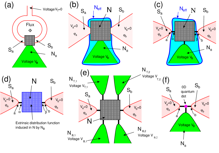
Figure 1: Schematics of the normal-superconducting Andreev interferometer: Panel a shows the experimental configuration of the normal-superconducting Andreev interferometer, including the external loop connecting $S_{a}$ and $S_{b}$, pierced by the magnetic flux $\Phi$, and the control parameter of the voltage bias $V_{B}$ on the normal lead $N_{B}$. Three of the considered theoretical modelings discussed in the paper are shown on panel b, c and d, including multichannel interfaces (b), single-channel contacts (c) and an effective model for the populations in the sequential tunneling channel (d). A normal-superconducting Andreev interferometer with four normal leads is shown on panel e. The theoretical device geometries on panels b-e are physically introduced in section II.2. A device with a quantum dot is also shown (f), corresponding to the simple 0D model solved in the Appendix C.

Figure 2: Schematics of the infinite planar geometry: The device consists of an infinite 2D normal metallic lead connected to the two superconductors $S_{a}$ and $S_{b}$ by small-area interfaces. Those normal-superconducting contacts could be realized by evaporating the superconducting lead on top of an insulator containing two holes. We show a top view of the device on panel a and a cut on panel b. The infinite 2D metallic lead is biased at the voltage $V_{B}$. Contrary to the devices shown in figure 1, this infinite planar configuration does not sustain geometrical resonances in the absence of coupling to the superconducting leads. The corresponding calculations are presented in section IV.3.

II Hamiltonians, geometry and method

In this section, we present the technical background of the paper: the Hamiltonians (see subsection II.1) and the geometry (see subsection II.2). More details about the methods are presented in the Appendix A that is summarized in section II.3.

II.1 Hamiltonians

In this subsection, we present the Hamiltonians of the superconducting and normal leads, and the coupling between them.

The superconducting leads are described by the standard BCS Hamiltonian with the gap $\Delta$, the bulk hopping amplitude $W$ and the superconducting phase variable $\varphi_{k}$:

$$\hat{\cal H}_{BCS} = -W\sum_{\langle i,j\rangle}\sum_{\sigma_{z}=\uparrow,\downarrow}\left(c_{i,\sigma_{z}}^{+}c_{j,\sigma_{z}}+c_{j,\sigma_{z}}^{+}c_{i,\sigma_{z}}\right)$$ (1)

$$- \Delta\sum_{k}\left(\exp\left(i\varphi_{k}\right)c_{k,\uparrow}^{+}c_{k,\downarrow}^{+}+\exp\left(-i\varphi_{k}\right)c_{k,\downarrow}c_{k,\uparrow}\right),$$ (2)

where spin-$\sigma_{z}$ electrons have the opportunity to be transferred with amplitude $W$ between the neighboring tight-binding site $\langle i,j\rangle$ on a lattice. In addition to the kinetic energy, the pairing term with amplitude $\Delta$ binds opposite-spin electrons with the phase $\varphi_{k}$, taken as uniform within each superconducting lead, i.e. $\varphi_{k}=\varphi_{a}$ or $\varphi_{k}=\varphi_{b}$ in the superconducting lead $S_{a}$ or $S_{b}$ respectively.

The normal-metallic parts of the Andreev interferometers are captured by a square-lattice tight-binding model with the bulk hopping amplitude $W$:

$$\hat{\cal H}_{N}=-W\sum_{\langle i,j\rangle}\sum_{\sigma_{z}=\uparrow,\downarrow}\left(c_{i,\sigma_{z}}^{+}c_{j,\sigma_{z}}+c_{j,\sigma_{z}}^{+}c_{i,\sigma_{z}}\right),$$ (3)

where we use for simplicity in Eq. (3) the same hopping amplitude $W$ as in Eq. (1) for the kinetic term of the BCS Hamiltonian. The summation in Eq. (3) runs over all pairs of neighboring tight-binding sites in the finite central normal conductor or in the infinite normal lead $N_{B}$, depending on which part of the circuit is described.

The tunneling term couples the leads $L_{1}$ and $L_{2}$ according to

$$\hat{\cal H}_{L_{1},L_{2}}=-t\sum_{\langle i,j\rangle}\sum_{\sigma_{z}=\uparrow,\downarrow}\left(c_{i,\sigma_{z}}^{+}c_{j,\sigma_{z}}+c_{j,\sigma_{z}}^{+}c_{i,\sigma_{z}}\right),$$ (4)

where $i$ and $j$ belong to the $L_{1}$ and $L_{2}$ sides of the interfaces respectively.

II.2 Andreev interferometer geometries

In this subsection, we present the different geometries that are investigated in the paper.

The normal-superconducting Andreev interferometer shown in Fig. 1a consists of a large superconducting loop that is edge-connected to an ultraclean 2D normal metal in the long- or intermediate-junction limit, i.e. the 2D normal metal linear dimension $L\gtrsim\xi_{0}$ exceeds the ballistic superconducting coherence length $\xi_{0}=\hbar v_{F}/\Delta$, where $v_{F}$ is the Fermi velocity and the superconducting gap $\Delta$ was defined in Eq. (2). We denote by $S_{a}$ and $S_{b}$ the two left and right end-lines of the superconducting loop connected to the 2D normal metal at the $S_{a}$-$N$ and $N$-$S_{b}$ interfaces respectively. As discussed in the Introduction, a normal lead $N_{B}$ is connected at the bottom to the 2D normal metal, forming the $N_{B}$-$N$ interface. A dissipative current $I_{B}$ flows between $N_{B}$ and the grounded left and right $S_{a}$ and $S_{b}$, in response to the voltage $V_{B}$ on $N_{B}$.

The superconducting phase variables $\varphi_{a}$ and $\varphi_{b}$ of $S_{a}$ and $S_{b}$ are the following:

$$\varphi_{a} \simeq \varphi_{0}-\Phi/2$$ (5)

$$\varphi_{b} \simeq \varphi_{0}+\Phi/2,$$ (6)

with $\Phi$ the flux piercing through the superconducting loop. The overall phase variable $\varphi_{0}$ remains free, and all physical observables are independent of $\varphi_{0}$ because of gauge invariance. In the above Eqs. (5)-(6), we assumed that the radius of the external superconducting loop is much larger than the linear dimension $L$ of the 2D metal. Considering a closed contour encircling the superconducting loop, we neglect the line integral of the vector potential in the region sustained by the 2D normal metal.

In order to discuss the emergence of resonances in the normal-superconducting Andreev interferometers, we distinguish between:

(i) The absence of geometrical resonance if the normal metal $N$ is captured by a 2D normal lead extending to infinity: The geometry of the normal-superconducting Andreev interferometer in Fig. 2 is uniform in space if the superconducting leads are disconnected. As shown in the forthcoming section IV, lowest-order perturbation theory in the tunneling amplitudes with the superconductors produces a coupling to the 2D metal continuum, and the corresponding conductance $dI_{B}/dV_{B}$ does not show any sharp feature related to the geometrical resonances, which are not there in the infinite planar geometry. However, Fabry-Pérot oscillations between the superconducting contacts are possible at higher-order in tunneling with the superconductors, which is compatible with the inversion-noninversion alternations that we find at the lowest order in tunneling.

(ii) The integrable-billiard-like geometrical resonances in the finite-size central region $N$: In the absence of coupling to the superconducting leads, the quantum states of the finite-size $N$ are broadened by the coupling to the infinite $N_{B}$. Concerning the populations, we find that sequential tunneling couples to the $V_{B}$-sensitive jumps in the nonequilibrium distribution functions of the central normal-metallic region $N$, see the discussion in the Introduction. In the other limiting case of elastic cotunneling, the conductance $dI_{B}/dV_{B}$ also couples to processes on the $eV_{B}$ energy shell. All of the external lead chemical potentials are involved in the presence of coupling to several normal leads biased at different voltages, see the multiterminal configuration in Fig. 1e.

Further assumptions are made about the geometry, such as simplifying the multichannel contacts in Fig. 1b into the single-channel ones of Fig. 1c. In order to capture the qualitative physics, averaging is carried out over pairs of contact points at both interfaces in real space, see for instance Refs. theory-CPBS12, ; theory-CPBS11, ; theory-CPBS13, ; Floser, in connection with the ferromagnet-superconductor-ferromagnet or normal metal-superconductor-normal metal beam splitters.

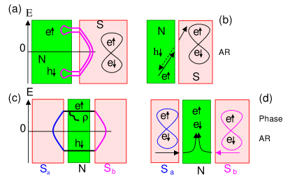
Figure 3: Schematics of the phase-AR process: Standard local Andreev reflection is shown on panels a and b. In local Andreev reflection, a spin-up electron is incoming from the $N$-side of the normal metal-superconductor $N$-$S$ interface, and a Cooper pair is transmitted into the condensate of $S$ while a spin-down hole is Andreev reflected in $N$. Panels c and d show the three-terminal process of phase-Andreev reflection (phase-AR), where the wavy line terminated by the symbol $\rho$ on panel c is a representation of the coupling to the density in $N$, via the nonlocal Keldysh Green’s function.

II.3 Methods

All of the necessary technical details about the methods are gathered in the Appendix A. Appendix A.1 presents the form of the advanced and retarded Green’s functions. Appendix A.2 presents the large-gap approximation suitable to capture a small bias voltage $V_{B}$ in the normal-superconducting Andreev interferometer shown in Fig. 1a. Appendix A.3 presents the assumptions about the population and Appendix A.4 explains how the current is calculated from the Keldysh Green’s functions.

In the following, we present our results.

III Elastic cotunneling and sequential tunneling

In this section, we evaluate how the electronic populations couple to the current. This will distinguish between the limiting cases of “dominant elastic cotunneling” and “dominant sequential tunneling”.

Current conservation: For simplicity, we start with a 0D quantum dot with broadened energy levels, as in Ref. Melin2017, . We assume that this 0D quantum dot $x$ is connected to the grounded left and right superconducting leads $S_{a}$ and $S_{b}$ respectively, and to the normal lead $N_{B}$ biased at the voltage $V_{B}$, see figure 1f. Then, using the Keldysh Green’s functions presented in the Appendix A, we find the following expression for $I_{a}+I_{b}$, the sum of the currents transmitted into $S_{a}$ and $S_{b}$:

$$I_{a}+I_{b} = \mbox{Nambu-trace}\left\{\left(\hat{\Gamma}_{x,x}^{A}\hat{\tau}_{3}-\hat{\tau}_{3}\hat{\Gamma}_{x,x}^{R}\right)\hat{G}^{+,-}_{x,x}\right.$$

$$+ \left.\hat{\Gamma}_{x,x}^{+,-}\hat{\tau}_{3}\hat{G}^{R}_{x,x}-\hat{\tau}_{3}\hat{\Gamma}_{x,x}^{+,-}\hat{G}^{A}_{x,x}\right\},$$

with

$$\hat{G}_{x,x}^{+,-} = \left(\hat{I}+\hat{G}{x,x}\hat{\Gamma}^{R}_{x,x}\right)\hat{g}^{+,-}_{x,x}\left(\hat{I}+\hat{\Gamma}^{A}_{x,x}\hat{G}^{A}_{x,x}\right)$$

$$+ \hat{G}^{R}_{x,x}\hat{\Gamma}^{+,-}_{x,x}\hat{G}^{A}_{x,x},$$

where we use the following notations

$$\hat{\Gamma}_{x,x}^{A} = \hat{t}_{x,a}\hat{g}^{A}_{a,a}\hat{t}_{a,x}+\hat{t}_{x,b}\hat{g}^{A}_{b,b}\hat{t}_{b,x}$$ (9)

$$\hat{\Gamma}_{x,x}^{R} = \hat{t}_{x,a}\hat{g}^{R}_{a,a}\hat{t}_{a,x}+\hat{t}_{x,b}\hat{g}^{R}_{b,b}\hat{t}_{b,x}$$ (10)

$$\hat{\Gamma}_{x,x}^{+,-} = \hat{t}_{x,a}\hat{g}^{+,-}_{a,a}\hat{t}_{a,x}+\hat{t}_{x,b}\hat{g}^{+,-}_{b,b}\hat{t}_{b,x}$$ (11)

and the Keldysh Green’s function is defined as $\hat{g}^{+,-}_{x,x}=n_{F}(\omega)\left[g^{A}_{x,x}-g^{R}_{x,x}\right]$. Using the identities

$$\hat{\Gamma}_{x,x}^{R}\hat{G}_{x,x}^{R} = \left(g^{R}_{x,x}\right)^{-1}\hat{G}^{R}_{x,x}-\hat{I}$$ (12)

$$\hat{G}_{x,x}^{A}\hat{\Gamma}_{x,x}^{A} = \hat{G}^{A}_{x,x}\left(g^{A}_{x,x}\right)^{-1}-\hat{I},$$ (13)

we obtain a simplified expression of $I_{a}+I_{b}$:

$$I_{a}+I_{b}=\mbox{Nambu-trace}\left\{\right.$$ (15)

$$\left(\hat{\Gamma}^{A}_{x,x}\hat{\tau}_{3}-\hat{\tau}_{3}\hat{\Gamma}_{x,x}^{R}\right)\left(\hat{I}+\hat{G}^{R}_{x,x}\hat{\Gamma}_{x,x}^{R}\right)\hat{g}^{+,-}_{x,x}\left(\hat{I}+\hat{\Gamma}_{x,x}^{A}\hat{G}_{x,x}^{A}\right)$$

$$+ \left.\hat{\tau}_{3}\hat{G}^{R}_{x,x}\hat{\Gamma}_{x,x}^{+,-}\hat{G}_{x,x}^{A}\left[\left(\hat{g}^{A}_{x,x}\right)^{-1}-\left(\hat{g}^{R}_{x,x}\right)^{-1}\right]\right\}.$$ (16)

The populations $n_{F}(\omega)$ of the central normal region at the energy $\omega$ are calculated from imposing the vanishingly small spectral current $I_{a}+I_{b}\equiv 0$, which makes $n_{F}(\omega)$ acquire jumps at each of the external normal reservoir chemical potential.

The following calculations will be carried in the following limiting cases: First, in the regime of “dominant elastic cotunneling”, the jumps in $n_{F}(\omega)$ contribute to the conductance $dI_{B}/dV_{B}$ according to Eq. (15). We will also consider the regime of “dominant elastic cotunneling” where the term in Eq. (16) is much larger than Eq. (15).

Multichannel contacts: Considering next a multilevel quantum dot connected to the collection of the leads $\{L_{p}\}$, we deduce from Appendix A that the spectral current flowing at the $D_{p}$-$L_{p}$ interface is given by

$$I_{p}=\mbox{Nambu-trace}\{\hat{\tau}_{3}\hat{t}_{L_{p},D_{p}}\hat{G}^{+,-}_{D_{p},L_{p}}-\hat{\tau}_{3}\hat{t}_{D_{p},L_{p}}\hat{G}^{+,-}_{L_{p},D_{p}}\},$$ (17)

where the bare advanced and retarded Green’s functions are given by

$$\hat{G}^{A}_{D_{p},L_{p}} = \hat{G}^{A}_{D_{p},D_{p}}\hat{t}_{D_{p},L_{p}}\hat{g}^{A}_{L_{p},L_{p}}$$ (18)

$$\hat{G}^{R}_{D_{p},L_{p}} = \hat{G}^{R}_{D_{p},D_{p}}\hat{t}_{D_{p},L_{p}}\hat{g}^{R}_{L_{p},L_{p}}$$ (19)

and the Keldysh Green’s function is given by

$$\hat{G}^{+,-}_{D_{p},L_{p}} = \hat{G}^{+,-}_{D_{p},D_{p}}\hat{t}_{D_{p},L_{p}}\hat{g}^{A}_{L_{p},L_{p}}+\hat{G}^{R}_{D_{p},D_{p}}\hat{t}_{D_{p},L_{p}}\hat{g}^{+,-}_{L_{p},L_{p}}.$$ (20)

We reach the same conclusions as above regarding sequential tunneling and elastic cotunneling because the single 0D tight-binding site $x$ in the above calculations now becomes the vector-valued $x\equiv\left(D_{1},\,...,\,D_{n}\right)$.

IV Inversion and phase-AR

In this section, we assume the absence of geometrical resonance and calculate the conductance $dI_{B}/dV_{B}$ defined by Eq. (96) as a function of the bias voltage $V_{B}$ applied to the normal lead $N_{B}$, where $I_{B}$ is the current flowing in $N_{B}$.

The microscopic process of phase-sensitive Andreev reflection (phase-AR) is presented in subsection IV.1. Subsection IV.2 deals with a general model for $N_{eff}$, whether or not it sustains geometrical resonances, see Fig. 1b, Fig. 1c, Fig. 1f and Fig. 2. We assume in subsection IV.3 an infinite planar 2D metal for $N$, without integrable-billiard-like geometrical resonances, see Fig. 2.

IV.1 Phase-Andreev reflection (phase-AR)

In this subsection, we physically introduce the process of phase-AR by which a normal current in the bottom $N_{B}$ is converted into a superconducting current in the loop, see Fig. 1a for the schematics of the normal-superconducting Andreev interferometer.

Such conversion is already operational in Andreev reflection Andreev ; BTK at a normal metal-insulator-superconductor (NIS) interface, see Fig. 3a and Fig. 3b. A spin-up electron incoming on the $N$ side is Andreev reflected as a spin-down hole while a Cooper pair is transmitted into the superconductor $S$ as an evanescent quasiparticle eventually joining the superconducting condensate Andreev ; BTK .

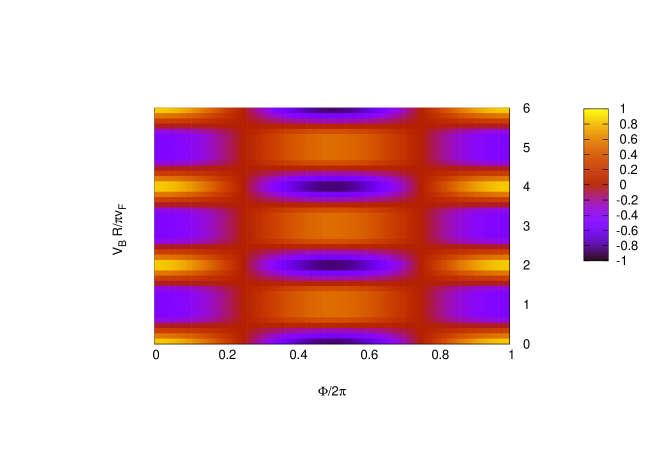
Figure 4: Colorplot of the normal-superconducting Andreev interferometer dimensionless conductance $g_{0}(\Phi/2\pi,V_{B}R/\pi\hbar v_{F})$ given by Eq. (31). We assume for simplicity a single jump in the distribution function of the central 2D metal, in the regime of dominant sequential tunneling. The dimensionless zero-temperature conductance $g_{0}\propto dI_{B}/dV_{B}$ is plotted as a function of the reduced magnetic flux $\Phi/2\pi$ (on the $x$-axis) and the reduced effective Fermi energy $y=V_{B}R/\pi\hbar v_{F}$ (on the $y$-axis). We obtain alternations between inversion and noninversion, where the dimensionless conductance $g_{0}$ is larger at the flux $\Phi=\pi$ than at $\Phi=0$ for the inversion, or the reverse for the noninversion.

We microscopically consider that a spin-up electron is Andreev reflected at one interface and the resulting spin-down hole is coherently transferred through ABS to the other interface where the spin-down hole is scattered into a spin-up electron, see Fig. 3c and Fig. 3d. We propose to use the wording phase-AR for the process shown in Fig. 3c and Fig. 3d in order to reflect the interplay between phase-sensitivity and the coupled spin-up electron/spin-down hole current conversions typical of AR. We argue that, microscopically, this density-phase coupling produces a transient coherent superposition between Cooper pairs (CPs) at each of the $S_{a}IN_{a}$ and $N_{b}IS_{b}$ interfaces, e.g. a superposition of the following type: $\left(|CP\,a\rangle\pm\exp(i\Phi)|CP\,b\rangle\right)/\sqrt{2}$.

Now, we discuss the parity of the conductance $dI_{B}/dV_{B}$ upon changing the signs of the voltage $V_{B}$ and the phase difference $\varphi_{b}-\varphi_{a}\simeq\Phi$. Let us first assume a tunnel contact between $N_{B}$ and the 2D metal $N$. Then, the differential conductance $dI_{B}/dV_{B}$ is proportional to the density of states (DOS) in $N$. The DOS of the ABS formed between $S_{a}$ and $S_{b}$ is even in the phase difference $\varphi_{b}-\varphi_{a}\simeq\Phi$ and thus, $dI_{B}/dV_{B}$ is also even in the magnetic flux $\Phi\simeq\varphi_{b}-\varphi_{a}$. The observation that $I_{B}$ changes sign if both $V_{B}$ and $\Phi\simeq\varphi_{b}-\varphi_{a}$ are simultaneously reversed implies that $I_{B}$ is odd in the voltage $V_{B}$ and $dI_{B}/dV_{B}$ is even in $V_{B}$.

IV.2 Expression of the tunneling conductance

In this subsection, we obtain a simple expression for the conductance $dI_{B}/dV_{B}$ in the limit of small contact transparencies.

The dissipative spectral current transmitted into $S_{a}$ [see Eq. (84] is expanded to the order-$t_{a}^{2}t_{b}^{2}$:

$$\hat{t}_{\alpha,a}\delta\hat{G}_{a,\alpha}^{+,-}(\omega)\simeq$$

$$\hat{t}_{\alpha,a}\hat{g}^{R}_{a,a}\hat{t}_{a,\alpha}\hat{g}^{R}_{\alpha,\beta}(\omega)\hat{t}_{\beta,b}\hat{g}^{R}_{b,b}\hat{t}_{b,\beta}\delta\hat{g}^{+,-}_{\beta,\alpha}(\omega)$$

$$+ \hat{t}_{\alpha,a}\hat{g}^{R}_{a,a}\hat{t}_{a,\alpha}\delta\hat{g}^{+,-}_{\alpha,\beta}(\omega)\hat{t}_{\beta,b}\hat{g}^{A}_{b,b}\hat{t}_{b,\beta}\hat{g}^{A}_{\beta,\alpha}(\omega),$$

and

$$\hat{t}_{a,\alpha}\delta\hat{G}_{\alpha,a}^{+,-}(\omega)\simeq$$

$$\hat{t}_{a,\alpha}\hat{g}^{R}_{\alpha,\beta}(\omega)\hat{t}_{\beta,b}\hat{g}^{R}_{b,b}\hat{t}_{b,\beta}\delta\hat{g}^{+,-}_{\beta,\alpha}(\omega)\hat{t}_{\alpha,a}\hat{g}^{A}_{a,a}$$

$$+ \hat{t}_{a,\alpha}\delta\hat{g}^{+,-}_{\alpha,\beta}(\omega)\hat{t}_{\beta,b}\hat{g}^{A}_{b,b}\hat{t}_{b,\beta}\hat{g}^{A}_{\beta,\alpha}(\omega)\hat{t}_{\alpha,a}\hat{g}^{A}_{a,a}.$$

The $\{\mu_{N,q}\}$-sensitive component of the spectral current takes the following form at the order-$t_{a}^{2}t_{b}^{2}$:

$$I_{a,\alpha}(\{\mu_{N,q}\},\{Z_{q}\},\omega)$$

$$= \mbox{Nambu-trace}\left\{\hat{\tau}_{3}\left[\hat{t}_{\alpha,a}(\ref{eq:(1)})-\hat{t}_{a,\alpha}(\ref{eq:(1)-prime})\right]\right\}$$

$$\equiv I_{0}(\{\mu_{N,q}\},\{Z_{q}\},\omega)+I_{1}(\{\mu_{N,q}\},\{Z_{q}\},\Phi,\omega),$$

where $Z_{q}$ is defined in the Appendix A.3 and we separate between the magnetic flux-$\Phi$-insensitive term $I_{0}(\{\mu_{N,q}\},\{Z_{q}\},\omega)$ of order-$t_{a}^{4}$ and the magnetic flux-$\Phi$ sensitive $I_{1}(\{\mu_{N,q}\},\{Z_{q}\},\Phi,\omega)$ coupling both interfaces, i.e. $I_{1}(\{\mu_{N,q}\},\{Z_{q}\},\Phi,\omega)$ is of order-$t_{a}^{2}t_{b}^{2}$:

$$I_{1}(\{\mu_{N,q}\},\{Z_{q}\},\Phi,\omega)$$

$$\simeq\mbox{Nambu-trace}\left\{\hat{\tau}_{3}\left[\hat{t}_{\alpha,a}\hat{g}^{R}_{a,a}\hat{t}_{a,\alpha}\hat{g}^{R}_{\alpha,\beta}(\omega)\hat{t}_{\beta,b}\hat{g}^{R}_{b,b}\hat{t}_{b,\beta}\delta\hat{g}^{+,-}_{\beta,\alpha}(\omega)\right.\right.$$

$$+ \hat{t}_{\alpha,a}\hat{g}^{R}_{a,a}\hat{t}_{a,\alpha}\delta\hat{g}^{+,-}_{\alpha,\beta}(\omega)\hat{t}_{\beta,b}\hat{g}^{A}_{b,b}\hat{t}_{b,\beta}\hat{g}^{A}_{\beta,\alpha}(\omega)$$

$$-\hat{t}_{a,\alpha}\hat{g}^{R}_{\alpha,\beta}(\omega)\hat{t}_{\beta,b}\hat{g}^{R}_{b,b}\hat{t}_{b,\beta}\delta\hat{g}^{+,-}_{\beta,\alpha}(\omega)\hat{t}_{\alpha,a}\hat{g}^{A}_{a,a}$$

$$- \left.\left.\hat{t}_{a,\alpha}\delta\hat{g}^{+,-}_{\alpha,\beta}(\omega)\hat{t}_{\beta,b}\hat{g}^{A}_{b,b}\hat{t}_{b,\beta}\hat{g}^{A}_{\beta,\alpha}(\omega)\hat{t}_{\alpha,a}\hat{g}^{A}_{a,a}\right]\right\}.$$

We make the Nambu labels explicit in the above Eq. (IV.2), and consider voltage or energy scales that are small compared to the superconducting gap, see Appendix A.2. Within this large-gap approximation, the spectral current $\tilde{I}_{1}(\{\mu_{N,q}\},\{Z_{q}\},\Phi,\omega)$ takes the following form at the order-$t_{a}^{2}t_{b}^{2}$:

$$\tilde{I}_{1}(\{\mu_{N,q}\},\{Z_{q}\},\Phi,\omega)\simeq$$

$$2\frac{t_{a}^{2}t_{b}^{2}}{W^{2}}e^{i\Phi}\left[\hat{g}^{R,2,2}_{\alpha,\beta}(\omega)\delta\hat{g}^{+,-,1,1}_{\beta,\alpha}(\omega)+\delta\hat{g}^{+,-,2,2}_{\alpha,\beta}(\omega)\hat{g}_{\beta,\alpha}^{A,1,1}(\omega)\right]$$

$$- 2\frac{t_{a}^{2}t_{b}^{2}}{W^{2}}e^{-i\Phi}\left[\hat{g}^{R,1,1}_{\alpha,\beta}(\omega)\delta\hat{g}^{+,-,2,2}_{\beta,\alpha}(\omega)+\delta\hat{g}^{+,-,1,1}_{\alpha,\beta}(\omega)\hat{g}_{\beta,\alpha}^{A,2,2}(\omega)\right],$$

where the superscripts “1” and “2” refer to the “spin-up electron” and “spin-down hole” Nambu components respectively. We further assume that the interfaces have transverse dimension that is much smaller than the distance between them. This assumption allows parameterizing the geometry with the single variable $R\equiv R_{\alpha,\beta}$ for the separation between the interfaces. A generalization to extended interfaces is possible, see the discussion concluding the above subsection II.2. For instance, one option is to sum over all the pairs of the tight-binding sites at both interfaces in the tunnel limit. At higher transparency, the Dyson matrices can be inverted, with entries in the set of the tight-binding sites making the contacts, see for instance Ref. theory-CPBS12, .

IV.3 Infinite planar geometry

In this subsection, we calculate the conductance $dI_{B}/dV_{B}$ of the phase-AR process within lowest-order perturbation theory in the tunneling amplitudes, and in the infinite planar geometry of figure 2.

Under those conditions, we deduce from Eq. (IV.2) the following expression for the spectral conductance $\partial\tilde{I}_{1}/\partial\mu_{N,p}(\omega)$ at the order-$t_{a}^{2}t_{b}^{2}$:

$$\frac{\partial\tilde{I}_{1}(\{\mu_{N,q}\},\{Z_{q}\},\Phi,\omega)}{\partial\mu_{N,p}}\simeq 8Z_{p}\frac{t_{a}^{2}t_{b}^{2}}{W^{4}\sqrt{k_{h}R}\sqrt{k_{e}R}}\cos\Phi\times$$ (26)

$$\cos\left(k_{h}R-\frac{\pi}{4}\right)\cos\left(k_{e}R-\frac{\pi}{4}\right)\times\left[\delta(\omega-\mu_{N,p})+\delta(\omega+\mu_{N,p})\right].$$

Approximating the slowly varying $\sqrt{k_{h}R}\sqrt{k_{e}R}$ as $k_{F}R$ in the prefactor and integrating over the energy $\omega$ leads to the following leading-order term in the expansion of $\partial\tilde{I}_{1}/\partial\mu_{N,p}(\omega)$ as a function of the hopping amplitudes $t_{a}$ and $t_{b}$:

$$\frac{\partial\tilde{I}_{1}(\{\mu_{N,q}\},\{Z_{q}\},\Phi)}{\partial\mu_{N,p}}=$$

$$\int d\omega\frac{\partial\tilde{I}_{1}(\{\mu_{N,q}\},\{Z_{q}\},\Phi,\omega)}{\partial\mu_{N,p}}$$

$$\simeq 16Z_{p}\frac{t_{a}^{2}t_{b}^{2}}{W^{4}(k_{F}R)}\cos\Phi\cos\left[\left(k_{F}-\frac{\delta\mu_{N,p}}{\hbar v_{F}}\right)R-\frac{\pi}{4}\right]\times$$

$$\cos\left[\left(k_{F}+\frac{\delta\mu_{N,p}}{\hbar v_{F}}\right)R-\frac{\pi}{4}\right].$$

We note that $\delta\mu_{N,p}R/\hbar v_{F}$ and $k_{F}R$ encode the slow and fast oscillations respectively. In a standard procedure theory-CPBS11 ; theory-CPBS12 ; theory-CPBS13 ; Floser , we average out those $(k_{F}R)$-oscillations in order to mimic multichannel contacts according to $\langle\langle\cos(x+A)\cos(x-A)\rangle\rangle=(\cos 2A)/2$, namely,

$$\langle\langle\cos(x+A)\cos(x-A)\rangle\rangle=$$ (28)

$$\langle\langle\left(\cos x\cos A-\sin x\sin A\right)\left(\cos x\cos A+\sin x\sin A\right)\rangle\rangle=$$

$$\cos^{2}A\langle\langle\cos^{2}x\rangle\rangle-\sin^{2}A\langle\langle\sin^{2}x\rangle\rangle=\frac{1}{2}\cos(2A),$$

where the slow and fast variables are denoted by $A=\delta\mu_{N,p}R_{1,2}/\hbar v_{F}$ and $x=k_{F}R_{1,2}-\pi/4$ respectively. We obtain the following expression for the conductance $\partial I_{1}/\partial\mu_{N,p}$ at the order-$t_{a}^{2}t_{b}^{2}$:

$$\frac{\partial\langle\langle\tilde{I}_{1}(\{\delta\mu_{N,q}\},\Phi)\rangle\rangle}{\partial(\delta\mu_{N,p})}=$$ (29)

$$\langle\langle\int d\omega\frac{\partial\tilde{I}_{1}(\{\mu_{N,q}\},\{Z_{q}\},\Phi,\omega)}{\partial\mu_{N,p}}\rangle\rangle\simeq$$

$$8Z_{p}\frac{t_{a}^{2}t_{b}^{2}}{W^{4}(k_{F}R)}\cos\Phi\cos\left(\frac{2\delta\mu_{N,p}R}{\hbar v_{F}}\right).$$

In order to illustrate this Eq. (29), we consider a simple $(S_{a},\,S_{b},\,N_{B})$ normal-superconducting Andreev interferometer where $(S_{a},\,S_{b})$ are grounded and $N_{B}$ is biased at the voltage $V_{B}$. Thus, we have a single $V_{B}$-sensitive step of height $Z$ at the step-energy $\delta\mu_{N}=eV_{B}$ in the distribution function of the normal lead $N$. Eq. (29) then simplifies as follows:

$$\frac{\partial\langle\langle\tilde{I}_{1}(V_{B},\Phi)\rangle\rangle}{\partial V_{B}}\simeq 8Z\frac{t_{a}^{2}t_{b}^{2}}{W^{4}(k_{F}R)}g_{0}\left(\frac{\Phi}{2\pi},\frac{V_{B}R}{\pi\hbar v_{F}}\right),$$ (30)

where the dimensionless conductance $g_{0}$ is the following:

$$g_{0}\left(\frac{\Phi}{2\pi},\frac{V_{B}R}{\pi\hbar v_{F}}\right)=\cos\Phi\cos\left(\frac{2eV_{B}R}{\hbar v_{F}}\right).$$ (31)

Fig. 4 shows a color-plot for the conductance $g_{0}$ in the plane of the parameters $\Phi/2\pi$ and $V_{B}R/\pi\hbar v_{F}$. We conclude the emergence of multiple inversion-noninversion coherent alternations, as it was anticipated in the Introduction.

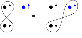
Figure 5: Schematics of the exchange between a pair and a single-particle electronic state. On this figure, we illustrate the anticommutation relations given by Eqs. (32)-(34). The left-hand-side of the cartoon shows the paired $c_{x,\uparrow}^{+}c_{x,\downarrow}^{+}$ and the single-particle $c_{y,\uparrow}^{+}$. The right-hand-side shows the rearrangement as the single-particle $c_{x,\uparrow}^{+}$ and the paired $c_{y,\uparrow}^{+}c_{x,\downarrow}^{+}$. Note the “minus” sign in front of the right-hand-side cartoon, which reflects Eq. 34.

IV.4 Further physical remarks

In this subsection, we present physical remarks as an interpretation of the above Eq. (31).

Exchange between the ABS and the normal single-particle background: Let us consider an Andreev pair entering the normal metal $N$, which consists of a spin-up electron and a time-reversed spin-down hole. We denote this quantum state as $\left(c_{x,\uparrow}^{+}c_{x,\downarrow}^{+}\right)$, where $c_{x,\sigma}^{+}$ creates a spin-$\sigma$ electron at the location $x$. We also add another unpaired spin-up electron at the location $y$, corresponding to $c_{y,\uparrow}^{+}$. Then, the fermionic anticommutation relations lead to

$$\left(c_{x,\uparrow}^{+}c_{x,\downarrow}^{+}\right)c_{y,\uparrow}^{+} = c_{x,\uparrow}^{+}c_{x,\downarrow}^{+}c_{y,\uparrow}^{+}$$ (32)

$$= -c_{x,\uparrow}^{+}c_{y,\uparrow}^{+}c_{x,\downarrow}^{+}$$ (33)

$$= -c_{x,\uparrow}^{+}\left(c_{y,\uparrow}^{+}c_{x,\downarrow}^{+}\right),$$ (34)

where the pair $\left(c_{x,\uparrow}^{+}c_{x,\downarrow}^{+}\right)$ in Eq. (32) exchanges its spin-up component with the single-particle electronic state $c_{y,\uparrow}^{+}$, leading to Eq. (34). In the final state, a spin-up electron $c_{x,\uparrow}^{+}$ is separated, and the pair $\left(c_{y,\uparrow}^{+}c_{x,\downarrow}^{+}\right)$ is formed. We conclude that a minus sign is produced if a pair is exchanged with a single electron, see Fig. 5. The coupling to the density via the Keldysh Green’s function is nonequilibrium, which explains the noninversion at $V_{B}=0$ on figure 4 and the threshold voltage to produce the inversion.

Voltage dependence: The voltage-$V_{B}$-sensitive alternations can be viewed as a simple consequence of the oscillating $\exp(2iE\tau/\hbar)$, where the bias voltage energy is $E=eV_{B}$, with $\tau=R/v_{F}$ the delay for ballistic propagation between the $S_{a}$-$N_{\alpha}$ and the $N_{\beta}$-$S_{b}$ interfaces. The phase-AR current transmitted from $N_{B}$ towards $(S_{a},\,S_{b})$ is proportional to $\sim\cos\Phi$, see the above Eq. (31), instead of $\sim\sin\Phi$ for the equilibrium DC-Josephson current transmitted between $S_{a}$ and $S_{b}$. We also note that Eq. (31) reveals the ballistic undamped $\cos\left(2ER/\hbar v_{F}\right)$ alternations.

Comparison to the diffusive limit: In the diffusive limit, the elastic mean free path is large compared to the Fermi wave-length but small compared to the dimension of the device. It was established Pfeffer2014 ; Wilhelm ; Nakano ; Zaitsev ; Kadigrobov ; Volkov ; Nazarov1 ; Nazarov2 ; Yip ; Belzig ; Zaikin1 ; Zaikin2 ; Zaikin3 ; Zaikin4 that, in the diffusive limit, the conductance shows damped oscillations as a function of the bias voltage $V_{B}$, which are controlled by the Thouless energy, see also the recent experiment in Ref. Margineda, . This contrasts with the absence of damping in Eq. (31) as a function of the bias voltage.

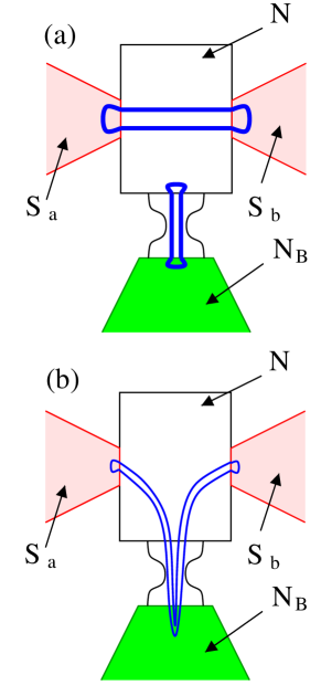
Figure 6: Schematics of the microscopic processes involved in sequential tunneling (a) and in elastic cotunneling (b), where the nonlocal Green’s functions have been gathered in a pairwise manner and a quantum point contact (QPC) is connected to the 2D metal $N$ and to the normal lead $N_{B}$. Sequential tunneling on panel a requires a finite density of states in the 2D normal metal N, and involves microscopic processes taking place locally at each interface. Elastic cotunneling on panel b involves a single higher-order tunneling diagram that crosses at least four times the $N$-$N_{B}$ interface through the QPC. Thus, the evolution of the conductance $dI_{B}/dV_{B}$ as a function of the opening of the QPC is a way to distinguish between sequential tunneling and elastic cotunneling. The former contributes to $dI_{B}/dV_{B}$ as $G_{B}$, whereas the latter contributes as $G_{B}^{2}$, where $G_{B}$ is the normal-state conductance of the $N$-QPC-$N_{B}$ interface.

How to experimentally distinguish between sequential tunneling and elastic cotunneling: The microscopic processes of elastic cotunneling and sequential tunneling are schematically shown in Fig. 6a and Fig. 6b respectively. Considering sequential tunneling on Fig. 6a, the current transmitted into $N$ is given by

$$I_{N}=(G_{a}+G_{b})\mu_{N}+G_{B}(\mu_{N}-V_{B})+G_{a,b}\mu_{N}\cos\Phi,$$ (35)

where $G_{a}$ and $G_{b}$ are the Andreev reflection conductances of each $S_{a}$-$N$ and $N$-$S_{b}$ interfaces, and $G_{B}$ is the conductance of the $N$-QPC-$N_{B}$ interface, where we assume that a quantum point contact (QPC) with tunable transparency has been inserted in between $N$ and $N_{B}$. Imposing the current conservation $I_{N}=0$ yields the expression of the normal metal Fermi energy

$$\mu_{N}=\frac{G_{B}}{G_{a}+G_{b}+G_{B}+G_{a,b}\cos\Phi}V_{B}.$$ (36)

The current transmitted into $N_{B}$ is then given by

$$I_{B} = G_{B}(V_{B}-\mu_{N})$$ (37)

$$= G_{B}\frac{G_{a}+G_{b}+G_{a,b}\cos\Phi}{G_{a}+G_{b}+G_{B}+G_{a,b}\cos\Phi}V_{B}$$ (38)

and, at the lowest order in the tunneling amplitude connecting the bottom $N_{B}$, the conductance $I_{B}/V_{B}$ scales like $I_{B}/V_{B}\sim G_{B}$, where $G_{B}$ is the normal-state conductance of the $N$-QPC-$N_{B}$ interface. This differs from the $I_{B}/V_{B}\sim G_{B}^{2}$ scaling of the elastic cotunneling process in Fig. 6b. Plotting the conductance $dI_{B}/dV_{B}$ as a function of both the bias voltage $V_{B}$ and the normal-state conductance is thus a way to experimentally determine whether the sequential tunneling or elastic cotunneling is dominant.

V Intrinsic resonances

In this section, we address resonances in geometries where an integrable billiard is connected to two superconducting leads and to a normal lead. We show how the intrinsic resonances of purely electronic origin emerge in those ultraclean multiterminal Josephson junctions, in the absence of coupling to the modes of the electromagnetic field as it is the case for the Fiske resonances Fiske .

Subsections V.1 and V.2 present calculations of the current associated to the one- and two-particle resonances within the dominant sequential tunneling mechanism. Subsection V.3 discusses dominant elastic cotunneling.

V.1 One-particle resonances

In this subsection, we assume the dominant sequential tunneling channel and address the emergence of the one-particle resonances in the expression of the current, on the basis of the calculation that is detailed in Appendix B. We assume that the “central” normal metal $N$ is connected to the superconductors $S_{a}$, $S_{b}$ and to the normal lead $N_{B}$ by contacts having arbitrary transmission.

In Appendix B, we find eight terms containing a single fully dressed Green’s function, see Eqs. (108), (108), (111), (114) and Eqs. (121), (121), (124), (127). Using the cyclic properties of the trace, the summation over those eight terms takes the following compact form:

$$I_{a}^{(1)}(\Phi,\omega)=\mbox{Nambu-trace}\left\{\sum_{k}\hat{t}_{\alpha,a}\left[\hat{\tau}_{3}\hat{g}^{R}_{a,a}-\hat{g}^{A}_{a,a}\hat{\tau}_{3}\right]\hat{t}_{a,\alpha}\times\right.$$ (39)

$$\left.\hat{G}^{R}_{\alpha,\alpha_{k}}(\omega)\hat{t}_{\alpha_{k},a_{k}}\hat{g}^{R}_{a_{k},a_{k}}\hat{t}_{a_{k},\alpha_{k}}\delta\hat{g}^{+,-}_{\alpha_{k},\alpha}(\omega)\right\}$$

$$+ \mbox{Nambu-trace}\left\{\sum_{k}\hat{t}_{\alpha,a}\left[\hat{\tau}_{3}\hat{g}^{R}_{a,a}-\hat{g}^{A}_{a,a}\hat{\tau}_{3}\right]\hat{t}_{a,\alpha}\times\right.$$

$$\left.\delta\hat{g}^{+,-}_{\alpha,\alpha_{k}}(\omega)\hat{t}_{\alpha_{k},a_{k}}\hat{g}^{A}_{a_{k},a_{k}}\hat{t}_{a_{k},\alpha_{k}}\hat{G}^{A}_{\alpha_{k},\alpha}(\omega)\right\}.$$

First coming back to the tunnel limit $t_{a,\alpha},\,t_{b,\beta}\ll W$, we replace the fully dressed Green’s functions $\hat{G}_{\alpha_{k},\alpha_{l}}$ by the bare ones $\hat{g}_{\alpha_{k},\alpha_{l}}$ and expand the Nambu labels according to

$$\tilde{I}_{a}^{(1)}(\Phi,\omega)=$$

$$2\hat{t}_{\alpha,a}^{1,1}\hat{g}^{R,1,2}_{a,a}\hat{t}_{a,\alpha}^{2,2}\hat{g}^{R,2,2}_{\alpha,\beta}(\omega)\hat{t}_{\beta,b}^{2,2}\hat{g}^{R,2,1}_{b,b}\hat{t}_{b,\beta}^{1,1}\delta\hat{g}^{+,-,1,1}_{\beta,\alpha}(\omega)$$

$$- 2\hat{t}_{\alpha,a}^{2,2}\hat{g}^{R,2,1}_{a,a}\hat{t}_{a,\alpha}^{1,1}\hat{g}^{R,1,1}_{\alpha,\beta}(\omega)\hat{t}_{\beta,b}^{1,1}\hat{g}^{R,1,2}_{b,b}\hat{t}_{b,\beta}^{2,2}\delta\hat{g}^{+,-,2,2}_{\beta,\alpha}(\omega)$$

$$+ 2\hat{t}_{\alpha,a}^{1,1}\hat{g}^{R,1,2}_{a,a}\hat{t}_{a,\alpha}^{2,2}\delta\hat{g}^{+,-,2,2}_{\alpha,\beta}(\omega)\hat{t}_{\beta,b}^{2,2}\hat{g}^{A,2,1}_{b,b}\hat{t}_{b,\beta}^{1,1}\hat{g}^{A,1,1}_{\beta,\alpha}(\omega)$$

$$- 2\hat{t}_{\alpha,a}^{2,2}\hat{g}^{R,2,1}_{a,a}\hat{t}_{a,\alpha}^{1,1}\delta\hat{g}^{+,-,1,1}_{\alpha,\beta}(\omega)\hat{t}_{\beta,b}^{1,1}\hat{g}^{A,1,2}_{b,b}\hat{t}_{b,\beta}^{2,2}\hat{g}^{A,2,2}_{\beta,\alpha}(\omega).$$

This Eq. (V.1) implies the above Eq. (IV.2). Thus, the phase-AR process evaluated in the above section IV is entirely within this one-particle sector.

Now, we consider the one-particle resonances and insert the fully dressed Green’s functions $\hat{G}^{A}_{\alpha_{k},\alpha_{l}}(\omega)$ and $\hat{G}^{R}_{\alpha_{k},\alpha_{l}}(\omega)$ into Eq. (39).

The fully dressed advanced and retarded Green’s functions have poles at the ABS energies $\Omega_{\lambda}\pm i\eta_{\lambda}$. The corresponding line-width broadening are denoted by $\eta_{\lambda}=\hbar/\tau_{\lambda}$, where $\tau_{\lambda}$ is the life-time of the ABS labeled by $\lambda$. Then, the fully dressed Green’s functions have the following spectral representation:

$$\hat{G}^{A}_{\alpha_{k},\alpha_{l}}(\omega) = \sum_{\lambda}\frac{\hat{\cal R}_{\alpha_{k},\alpha_{l}}^{(\lambda)}}{\omega-\Omega_{\lambda}-i\eta_{\lambda}}$$ (41)

and

$$\hat{G}^{R}_{\alpha_{k},\alpha_{l}}(\omega) = \sum_{\lambda}\frac{\hat{\cal R}_{\alpha_{k},\alpha_{l}}^{(\lambda)}}{\omega-\Omega_{\lambda}+i\eta_{\lambda}},$$ (42)

where $\hat{\cal R}$ is the matrix of the residues.

Conversely, in the absence of coupling to the superconductors, the bare Green’s functions of the normal metal $N$ connected to $N_{B}$ have the following spectral representation:

$$\hat{g}^{A}_{\alpha_{k},\alpha_{l}}(\omega) = \sum_{\mu}\frac{\hat{\cal R}_{\alpha_{k},\alpha_{l}}^{{}^{\prime}(\mu)}}{\omega-\zeta^{\prime}_{\mu}-i\eta^{\prime}_{\mu}}$$ (43)

and

$$\hat{g}^{R}_{\alpha_{k},\alpha_{l}}(\omega) = \sum_{\mu}\frac{\hat{\cal R}_{\alpha_{k},\alpha_{l}}^{{}^{\prime}(\mu)}}{\omega-\zeta^{\prime}_{\mu}+i\eta^{\prime}_{\mu}},$$ (44)

where $\eta^{\prime}_{\mu}$ is the corresponding line-width broadening. Eqs. (43)-(44) lead to the following expression for the derivative of the Keldysh Green’s function with respect to $\mu_{N,p}$:

$$\frac{\partial}{\partial\mu_{N,p}}\hat{g}^{+,-}_{\alpha_{k},\alpha_{l}}(\omega)$$

$$= 2i\pi Z_{p}\hat{\tau}_{3}\delta\left(\omega-\mu_{N,p}\hat{\tau}_{3}\right)\sum_{\mu}\hat{\cal R}_{\alpha_{k},\alpha_{l}}^{{}^{\prime}(\mu)}\delta_{\eta^{\prime}_{\mu}}\left(\omega-\zeta^{\prime}_{\mu}\right),$$

where $\delta_{\eta^{\prime}_{\mu}}$ is the Dirac $\delta$-function broadened by the line-width $\eta^{\prime}_{\mu}$.

Now, we insert Eqs. (41)-(V.1) into Eqs. (39). Then, $\partial\tilde{I}_{1}/\partial\mu_{N,p}$ takes the following form:

$$\frac{\partial}{\partial\mu_{N,p}}\int d\omega\tilde{I}_{a}^{(1)}(\Phi,\omega)=$$

$$4i\pi Z_{p}\mbox{Nambu-trace}\left\{\sum_{\lambda,\mu}\hat{t}_{\alpha,a}\hat{\tau}_{3}\hat{g}_{a,a}\hat{t}_{a,\alpha}\hat{\cal R}^{(\lambda)}_{\alpha,\beta}\hat{t}_{\beta,b}\hat{g}_{b,b}\hat{t}_{b,\beta}\times\right.$$

$$\left.\hat{\tau}_{3}\hat{\cal R}^{{}^{\prime}(\mu)}_{\beta,\alpha}\int d\omega\frac{\delta\left(\omega-\mu_{N,p}\hat{\tau}_{3}^{\beta,\alpha}\right)\delta_{\eta^{\prime}_{\mu}}\left(\omega-\zeta^{\prime}_{\mu}\right)}{\omega-\Omega_{\lambda}+i\eta_{\lambda}}\right\}$$

$$+ 4i\pi Z_{p}\mbox{Nambu-trace}\left\{\sum_{\lambda,\mu}\hat{t}_{\alpha,a}\hat{\tau}_{3}\hat{g}_{a,a}\hat{t}_{a,\alpha}\hat{\cal R}^{{}^{\prime}(\lambda)}_{\alpha,\beta}\hat{t}_{\beta,b}\hat{g}_{b,b}\hat{t}_{b,\beta}\times\right.$$

$$\left.\hat{\tau}_{3}\hat{\cal R}^{(\mu)}_{\beta,\alpha}\int d\omega\frac{\delta\left(\omega-\mu_{N,p}\hat{\tau}_{3}^{\alpha,\beta}\right)\delta_{\eta^{\prime}_{\lambda}}\left(\omega-\zeta^{\prime}_{\lambda}\right)}{\omega-\Omega_{\mu}-i\eta_{\mu}}\right\},$$

where we denoted by $g_{a,a}\equiv g^{A}_{a,a}=g^{R}_{a,a}$ and $g_{b,b}\equiv g^{A}_{b,b}=g^{R}_{b,b}$ the local superconducting Green’s function of $S_{a}$ and $S_{b}$ in the large-gap approximation and we then used $\hat{\tau}_{3}\hat{g}^{R}_{a,a}-\hat{g}^{A}_{a,a}\hat{\tau}_{3}=2\hat{\tau}_{3}\hat{g}_{a,a}$. The superscript on the matrix $\hat{\tau}_{3}$ refers to where it has been inserted in the chain of the Green’s function.

We conclude from the above Eq. (V.1) that this energy-integral is sensitive to the values of the complex energies $\zeta^{\prime}_{\mu}\pm i\eta^{\prime}_{\mu}$ of $N$ connected to $N_{B}$, and to the values of the fully dressed ABS energies $\Omega_{\lambda}\pm i\eta_{\lambda}$ in the presence of all couplings to the superconducting and normal leads $S_{a}$, $S_{b}$ and $N_{B}$ respectively.

V.2 Two-particle resonances

In this subsection, we assume the dominant sequential tunneling channel and discuss the emergence of two-particle resonances which will turn out to have stronger amplitude than the one-particle ones.

We obtain in Appendix B eight terms corresponding to the second-order contribution $I_{a}^{(2)}(\Phi,\omega)$ to the spectral current $I_{a}(\Phi,\omega)$, see Eqs. (108), (111), (114), (116) and Eqs. (121), (124), (127), (129). Using the cyclic properties of the trace, those contributions are summarized as follows:

$$I_{a}^{(2)}(\Phi,\omega)=\mbox{Nambu-trace}\left\{\sum_{k,l}\hat{t}_{\alpha,a}\left[\hat{\tau}_{3}\hat{g}^{R}_{a,a}-\hat{g}^{A}_{a,a}\hat{\tau}_{3}\right]\hat{t}_{a,\alpha}\times\right.$$ (47)

$$\left.\hat{G}^{R}_{\alpha,\alpha_{k}}(\omega)\hat{t}_{\alpha_{k},a_{k}}\hat{g}^{R}_{a_{k},a_{k}}\hat{t}_{a_{k},\alpha_{k}}\delta\hat{g}^{+,-}_{\alpha_{k},\alpha_{l}}(\omega)\hat{t}_{\alpha_{l},a_{l}}\hat{g}^{A}_{a_{l},a_{l}}\hat{t}_{a_{l},\alpha_{l}}\hat{G}^{A}_{\alpha_{l},\alpha}(\omega)\right\},$$

where Eq. (47) generally holds for arbitrary values of the tunneling amplitudes $t_{a}$ and $t_{b}$ connecting by single channel contacts the central normal metal to the superconducting leads $S_{a}$ and $S_{b}$.

Now, we insert into Eq. (47) the spectral decomposition given by Eqs. (41)-(V.1):

$$\frac{\partial}{\partial\mu_{N,p}}\int d\omega\tilde{I}_{a}^{(2)}(\Phi,\omega)=4i\pi Z_{p}\mbox{Nambu-trace}\left\{\sum_{k,l}\sum_{\lambda,\lambda^{\prime},\mu}\hat{t}_{\alpha,a}\hat{\tau}_{3}\right.$$

$$\left.\hat{g}_{a,a}\hat{t}_{a,\alpha}\hat{\cal R}^{(\lambda)}_{\alpha,\alpha_{k}}\hat{t}_{\alpha_{k},a_{k}}\hat{g}_{a_{k},a_{k}}\hat{t}_{a_{k},\alpha_{k}}\hat{\tau}_{3}\hat{\cal R}_{\alpha_{k},\alpha_{l}}^{{}^{\prime}(\mu)}\hat{t}_{\alpha_{l},a_{l}}\hat{g}_{a_{l},a_{l}}\hat{t}_{a_{l},\alpha_{l}}\hat{\cal R}^{(\lambda^{\prime})}_{\alpha_{l},\alpha}\times\right.$$

$$\left.\int d\omega\frac{\delta\left(\omega-\mu_{N,p}\hat{\tau}_{3}^{\alpha_{k},\alpha_{l}}\right)\delta_{\eta^{\prime}_{\mu}}\left(\omega-\zeta^{\prime}_{\mu}\right)}{\left(\omega-\Omega_{\lambda}+i\eta_{\lambda}\right)\left(\omega-\Omega_{\lambda^{\prime}}-i\eta_{\lambda^{\prime}}\right)}\right\},$$ (48)

where we also used $\hat{\tau}_{3}\hat{g}^{R}_{a,a}-\hat{g}^{A}_{a,a}\hat{\tau}_{3}=2\hat{\tau}_{3}\hat{g}_{a,a}$. As it was the case for the one-particle resonances, see Eq. (V.1), we find that the two-particle contribution to the current depends on the resonance energies $\Omega_{\lambda}$, $\Omega_{\lambda^{\prime}}$ and $\zeta^{\prime}_{\mu}$, see Eq. (48). This contribution is maximal if $\Omega_{\lambda}$ and $\Omega_{\lambda}^{\prime}$ are within the line-width broadening $\delta_{eff}$:

$$\Omega_{\lambda}=\Omega_{\lambda^{\prime}}+{\cal O}\left(\delta_{eff}\right).$$ (49)

In this sense, the spectrum of the two-particle resonances is sparse inside the spectrum of the pairs of one-particle resonances, on the condition of small line-width broadening $\delta_{eff}$, see the forthcoming section VI.1.

V.3 Further calculations of the two-particle resonances

In this subsection, we assume the dominant elastic cotunneling channel. We provide a complementary point of view on the two-particle resonances and directly evaluate the current $I_{B}$ flowing through the lead $N_{B}$:

$$I_{B}=\mbox{Nambu-trace}\left\{\hat{\tau}_{3}\left[\hat{\Sigma}_{N_{B},N}\hat{G}^{+,-}_{N,N_{B}}-\hat{\Sigma}_{N,N_{B}}\hat{G}^{+,-}_{N_{B},N}\right]\right\}.$$ (50)

We find the following for each of the Nambu components of $\hat{\Sigma}_{N_{B},N}\hat{G}^{+,-}_{N,N_{B}}$ and $\hat{\Sigma}_{N,N_{B}}\hat{G}^{+,-}_{N_{B},N}$:

$$\left(\hat{\Sigma}_{N_{B},N}\hat{G}^{+,-}_{N,N_{B}}\right)^{1,1}=\Sigma_{N_{B},N}^{1,1}G^{R,1,1}_{N,N}\Sigma_{N,N_{B}}^{1,1}g^{+,-,1,1}_{N_{B},N_{B}}$$ (51)

$$+ \Sigma_{N_{B},N}^{1,1}G^{R,1,1}_{N,N}\Sigma_{N,N_{B}}^{1,1}g^{+,-,1,1}_{N_{B},N_{B}}\Sigma_{N_{B},N}^{1,1}G^{A,1,1}_{N,N}\Sigma_{N,N_{B}}^{1,1}g^{A,1,1}_{N_{B},N_{B}}$$ (52)

$$+ \Sigma_{N_{B},N}^{1,1}G^{R,1,2}_{N,N}\Sigma_{N,N_{B}}^{2,2}g^{+,-,2,2}_{N_{B},N_{B}}\Sigma_{N_{B},N}^{2,2}G^{A,2,1}_{N,N}\Sigma_{N,N_{B}}^{1,1}g^{A,1,1}_{N_{B},N_{B}},$$ (53)

$$\left(\hat{\Sigma}_{N_{B},N}\hat{G}^{+,-}_{N,N_{B}}\right)^{2,2}=\Sigma_{N_{B},N}^{2,2}G^{R,2,2}_{N,N}\Sigma_{N,N_{B}}^{2,2}g^{+,-,2,2}_{N_{B},N_{B}}$$ (54)

$$+ \Sigma_{N_{B},N}^{2,2}G^{R,2,2}_{N,N}\Sigma_{N,N_{B}}^{2,2}g^{+,-,2,2}_{N_{B},N_{B}}\Sigma_{N_{B},N}^{2,2}G^{A,2,2}_{N,N}\Sigma_{N,N_{B}}^{2,2}g^{A,2,2}_{N_{B},N_{B}}$$ (55)

$$+ \Sigma_{N_{B},N}^{2,2}G^{R,2,1}_{N,N}\Sigma_{N,N_{B}}^{1,1}g^{+,-,1,1}_{N_{B},N_{B}}\Sigma_{N_{B},N}^{1,1}G^{A,1,2}_{N,N}\Sigma_{N,N_{B}}^{2,2}g^{A,1,1}_{N_{B},N_{B}},$$ (56)

$$\left(\hat{\Sigma}_{N,N_{B}}\hat{G}^{+,-}_{N_{B},N}\right)^{1,1}=\Sigma_{N,N_{B}}^{1,1}g^{+,-,1,1}_{N_{B},N_{B}}\Sigma_{N_{B},N}^{1,1}G^{A,1,1}_{N,N}$$ (57)

$$+ \Sigma_{N,N_{B}}^{1,1}g^{R,1,1}_{N_{B},N_{B}}\Sigma_{N_{B},N}^{1,1}G^{R,1,1}_{N,N}\Sigma_{N,N_{B}}^{1,1}g^{+,-,1,1}_{N_{B},N_{B}}\Sigma_{N_{B},N}^{1,1}G^{A,1,1}_{N,N}$$ (58)

$$+ \Sigma_{N,N_{B}}^{1,1}g^{R,1,1}_{N_{B},N_{B}}\Sigma_{N_{B},N}^{1,1}G^{R,1,2}_{N,N}\Sigma_{N,N_{B}}^{2,2}g^{+,-,2,2}_{N_{B},N_{B}}\Sigma_{N_{B},N}^{2,2}G^{A,2,1}_{N,N},$$ (59)

and

$$\left(\hat{\Sigma}_{N,N_{B}}\hat{G}^{+,-}_{N_{B},N}\right)^{2,2}=\Sigma_{N,N_{B}}^{2,2}g^{+,-,2,2}_{N_{B},N_{B}}\Sigma_{N_{B},N}^{2,2}G^{A,2,2}_{N,N}$$ (60)

$$+ \Sigma_{N,N_{B}}^{2,2}g^{R,2,2}_{N_{B},N_{B}}\Sigma_{N_{B},N}^{2,2}G^{R,2,2}_{N,N}\Sigma_{N,N_{B}}^{2,2}g^{+,-,2,2}_{N_{B},N_{B}}\Sigma_{N_{B},N}^{2,2}G^{A,2,2}_{N,N}$$ (61)

$$+ \Sigma_{N,N_{B}}^{2,2}g^{R,2,2}_{N_{B},N_{B}}\Sigma_{N_{B},N}^{2,2}G^{R,2,1}_{N,N}\Sigma_{N,N_{B}}^{1,1}g^{+,-,1,1}_{N_{B},N_{B}}\Sigma_{N_{B},N}^{1,1}G^{A,1,2}_{N,N}.$$ (62)

We next assume that the $N_{B}$-$N$ contact has moderately small transparency. Considering low energy in comparison to the superconducting gap, we perform the following approximation in Eqs. (51)-(62):

$$G_{N,N}^{1,1} \simeq G_{N,N}^{(1),1,1}$$

$$+ G_{N,N}^{(1),1,1}\Sigma_{N,S}^{1,1}g_{S,S}^{1,2}\Sigma_{S,N}^{2,2}G_{N,N}^{(1),2,2}\Sigma_{N,S}^{2,2}g_{S,S}^{2,1}\Sigma_{S,N}^{1,1}G_{N,N}^{(1),1,1}$$

$$G_{N,N}^{1,2} \simeq G_{N,N}^{(1),1,1}\Sigma_{N,S}^{1,1}g_{S,S}^{1,2}\Sigma_{S,N}^{2,2}G_{N,N}^{(1),2,2},$$ (64)

where

$$\hat{G}^{(1),A}_{\alpha_{k},\alpha_{l}}(\omega) = \sum_{\mu}\frac{\hat{\cal R}_{\alpha_{k},\alpha_{l}}^{{}^{\prime\prime}(\mu)}}{\omega-\zeta^{\prime\prime}_{\mu}-i\eta^{\prime\prime}_{\mu}}$$ (65)

and

$$\hat{G}^{(1),R}_{\alpha_{k},\alpha_{l}}(\omega) = \sum_{\mu}\frac{\hat{\cal R}_{\alpha_{k},\alpha_{l}}^{{}^{\prime\prime}(\mu)}}{\omega-\zeta^{\prime\prime}_{\mu}+i\eta^{\prime\prime}_{\mu}}$$ (66)

are the Green’s function in the absence of coupling to the bottom normal lead $N_{B}$, and where $\zeta^{\prime\prime}_{\mu}$ and $\eta^{\prime\prime}_{\mu}$ are the corresponding ABS energies and line-width broadening. In the large-gap approximation, we obtain the following expression for the difference between Eq. (53) and Eq. (59):

$$(\ref{eq:(A3)})-(\ref{eq:(C3)}) = \mbox{Nambu-trace}\left\{\hat{\tau}_{3}^{1,1}\Sigma_{N,N_{B}}^{1,1}\left[g^{A,1,1}_{N_{B},N_{B}}-g^{R,1,1}_{N_{B},N_{B}}\right]\times\right.$$

$$\left.\Sigma_{N_{B},N}^{1,1}G^{(1),1,1,R}_{N,N}\Sigma_{N,S}^{1,1}g^{1,2}_{S,S}\Sigma_{S,N}^{2,2}G^{(1),2,2,R}_{N,N}\times\right.$$

$$\left.\Sigma_{N,N_{B}}^{2,2}g^{+,-,2,2}_{N_{B},N_{B}}\Sigma_{N_{B},N}^{2,2}G^{(1),2,2,A}_{N,N}\Sigma_{N,S}^{2,2}G^{(1),1,1,A}_{N,N}\right\},$$

and a similar equation holds for the difference between Eq. (56) and Eq. (62). The remaining term given by Eqs. (51)-(52), Eqs. (54)-(55), Eqs. (57)-(58) and Eqs. (60)-(61) contribute to the current in the “$1,1$” electron-electron channel in response to the “$1,1$” component of the Keldysh Green’s function $g^{+,-,1,1}$. Those quasiparticle terms contribute to coupling the effective Fermi surface in $N$ to the bias voltage $V_{B}$ if the density of states in $N$ is nonvanishingly small.

The product $G^{(1),1,1,R}_{N,N}G^{(1),2,2,R}_{N,N}G^{(1),2,2,A}_{N,N}G^{(1),1,1,A}_{N,N}$ between four Green’s functions of the $G^{(1)}$-type appears in the phase-AR current given by Eq. (V.3). Those four Green’s functions are maximally resonant if the pairs of the spin-up electron and spin-down hole ABS energies $\zeta^{\prime\prime}_{\mu}$ and $\zeta^{\prime\prime}_{\nu}$ are opposite, where the $\zeta^{\prime\prime}$s are the ABS energies in the absence of coupling to the bottom normal lead $N_{B}$. This argument further illustrates the “two-particle resonances” in the ultraclean normal-superconducting Andreev interferometer shown in Fig. 1a, in the sense of resonances in both of the spin-up electron and spin-down hole channels. This is in a qualitative agreement with the 0D quantum dot discussed in Appendix C.

VI Discussion and conclusion

In order to conclude the paper, we present a discussion in subsection VI.1 and final remarks in subsection VI.2

VI.1 Discussion

In this subsection, we discuss the possibility that our model of a $(S_{a},\,S_{b},\,N_{B})$ normal-superconducting Andreev interferometer biased at the voltages $(0,\,0,\,V_{B})$ can extrapolate to the all-superconducting $(S_{a},\,S_{b},\,S_{B})$ Andreev interferometer, also biased at $(0,\,0,\,V_{B})$.

We already noted in the Introduction that $\varphi_{b}-\varphi_{a}\simeq\Phi$ is the only static combination of the superconducting phase variables to which the DC-current couples. We also note the absence of DC-current of Cooper pairs transmitted from the bottom $S_{B}$ to the superconducting loop, due to energy conservation, see also the adiabatic limit in Appendix D. A strong approximation is to discard any coupling to the Cooper pairs in $S_{B}$, even in intermediate states. This produces the Giaver approximation, where Eq. (82) becomes

$$\hat{g}_{B,Giaver}^{A}(\Delta,\omega)=\frac{1}{W\sqrt{\Delta^{2}-(\omega-i\eta_{S})^{2}}}\times$$ (71)

$$\left(\begin{array}[]{cc}-(\omega-i\eta_{S})&0\\ 0&-(\omega-i\eta_{S})\end{array}\right).$$

This Eq. (71) is viewed as the starting point of perturbation theory in the time-periodic Floquet dynamics. Considering here the zero order of this perturbation theory, the low-energy density of states $\rho_{B,Giaver}=\eta_{S}/\Delta W$ of $N_{B,\,Giaver}$ is reduced by a factor $\eta_{S}/\Delta$ in comparison to the normal metal $N_{B}$, where $\eta_{S}$ is the Dynes parameter Kaplan ; Dynes ; Pekola1 ; Pekola2 of the superconductor $S_{B}$. The line-width of the intrinsic resonances are consequently reduced by a factor $\eta_{S}/\Delta$. This enhanced ABS life-time is a property of the suppressed normal density of states in the superconducting gap and thus, this protection from the short relaxation time in the quasiparticle continua is expected to generalize to the all-superconducting $(S_{a},\,S_{b},\,S_{B})$ Andreev interferometer biased at $(0,\,0,\,V_{B})$, which turns out to be fully compatible with Ref. Melin2017, .

VI.2 Conclusion

In this subsection, we present a summary of the paper and final remarks.

In this work, we proposed the microscopic theory of an ultraclean $(S_{a},S_{b},N_{B})$ normal-superconducting Andreev interferometer, where $S_{a}$ and $S_{b}$ are connected by a loop pierced by a magnetic flux $\Phi$, and $N_{B}$ is biased at the voltage $V_{B}$.

We found that the microscopic theory confirms all of the physical expectations presented in the Introduction:

Connecting an integrable billiard to the normal lead $N_{B}$ and to a two-terminal Josephson junction has two effects:

(i) Providing a finite line-width broadening to the ABS, then becoming resonances.

(ii) Producing in the regime of sequential tunneling a nonequilibrium effective Fermi surface in $N$, in the sense of a single or multiple jumps in the distribution function at an energy that is sensitive to the bias voltage $V_{B}$.

Then, in the infinite planar geometry, we obtained multiple alternations between inversion and noninversion as a function of the bias voltage $V_{B}$. The inversion corresponds to the conductance $dI_{B}/dV_{B}$ that is larger at the flux $\Phi=\pi$ than in zero magnetic field $\Phi=0$ respectively.

We found emergence of the one- and two-particle resonances in the conductance $dI_{B}/dV_{B}$ of the normal-superconducting Andreev interferometer. Those resonances are preexisting in the absence of coupling to the superconducting leads. Measuring the conductance of the superconducting device at the variable bias voltage $V_{B}$ then allows a kind of spectroscopy of those intrinsic resonances. This mechanism has no counterpart with two terminals, and contrasts with the Fiske resonances that are also operational with two terminals.

We have also shown that zero order in the terms producing the time-periodic dynamics implies emergence of long time scales and small line-width broadening, due to protection by the superconducting gap of $S_{B}$ from strong relaxation of the ABS in the normal continua. Future works include going beyond the Giaver approximation and considering the possibility of Floquet replica of those intrinsic resonances. However, given the relevance of the nonFloquet resonances that we find, the observation of the Floquet resonances appears to be highly challenging from the point of view of experiments realized with 2D metals. We will also come back in the near future to the quartets and Floquet theory in the three- or four-terminal configurations, in order to determine whether the present work has consequences in the Josephson channel. To conclude, the present theoretical work supports the proposed interpretation of the recent Penn State group experiment.

Appendix A Details about the methods

This Appendix contains the necessary details about the methods on which the paper relies. The structure of this Appendix is provided in the main text, see section II.3.

A.1 Advanced and retarded Green’s functions in the normal region of the circuit

In this subsection of Appendix A, we first provide the form of the bare Green’s function $\hat{g}_{i,j}(\omega)$, i.e. the Green’s functions of the central region with vanishingly small tunneling amplitudes to the superconducting or normal lead. In a second step, we provide an approximation to the Green’s function of $N_{eff}$ consisting of $N$ strongly coupled to $N_{B}$.

Open infinite planar 2D metal not sustaining geometrical resonances: The electronic Green’s functions of an infinite planar 2D metal treated in the continuous limit are given by

$$g^{A,1,1}(R,\omega) = -g^{R,1,1}(R)=\frac{i}{W}J_{0}(k_{e}R)$$ (72)

$$g^{A,2,2}(R,\omega) = -g^{R,2,2}(R)=\frac{i}{W}J_{0}(k_{h}R),$$ (73)

where $J_{0}$ is a Bessel function, $\omega$ is the energy, $k_{e}$ and $k_{h}$ denote the electron and hole Fermi wave-vectors $k_{e,h}=k_{F}\pm\delta\omega/\hbar v_{F}$, with $\delta\omega$ the energy with respect to the equilibrium chemical potential. The variable $R$ in Eqs. (72)-(73) denotes the separation in real space.

In the limit of large separation $R\equiv R_{\alpha,\beta}$ between $\alpha$ and $\beta$, i.e. $R\gg 1/k_{F}$, we find the following approximation to the nonlocal bare Green’s functions:

$$g^{A,1,1}(R,\omega) = -g^{R,1,1}(R,\omega)$$

$$\simeq \frac{i}{W\sqrt{k_{e}R}}\cos\left(k_{e}R-\frac{\pi}{4}\right)$$

$$g^{A,2,2}(R,\omega) = -g^{R,2,2}(R,\omega)$$

$$\simeq \frac{i}{W\sqrt{k_{h}R}}\cos\left(k_{h}R-\frac{\pi}{4}\right).$$

Finite 2D metal connected to infinite normal leads: Now, we carry out perturbation theory in the coupling to the superconducting leads. We denote by $N$ the finite-size central normal conductor, which is attached to both superconducting leads $S_{a}$ and $S_{b}$ at the left and right respectively, and, at the bottom, to the normal lead $N_{B}$. The corresponding hopping amplitudes are denoted by $\hat{t}_{N,S_{a}}$, $\hat{t}_{N,S_{b}}$ and $\hat{t}_{N,N_{b}}$ respectively, where the diagonal matrix $\hat{t}_{i,j}=(t_{i,j},\,-t_{i,j})$ has entries in Nambu and in the set of the the tight-binding sites at the interfaces, see Eq. (4).

The Dyson equations for the fully dressed $\hat{G}_{N,N}(\omega)$ take the following form:

$$\hat{G}_{N,N}(\omega) = \hat{g}_{N,N}(\omega)$$

$$+ \hat{g}_{N,N}(\omega)\hat{t}_{N,N_{B}}\hat{g}_{N_{B},N_{B}}\hat{t}_{N_{B},N}\hat{G}_{N,N}(\omega)$$

$$+ \sum_{k}\hat{g}_{N,N}(\omega)\hat{t}_{N,a_{k}}\hat{g}_{a_{k},a_{k}}\hat{t}_{a_{k},N}\hat{G}_{N,N}(\omega).$$

Perturbation theory in $t_{a_{k},N}^{2}$ leads to

$$\hat{G}_{N,N}(\omega)=\left(\left(\hat{G}^{(0)}_{N,N}\right)^{-1}(\omega)-\sum_{k}\hat{t}_{N,a_{k}}\hat{g}_{a_{k},a_{k}}\hat{t}_{a_{k},N}\right)^{-1},$$ (77)

where $\hat{G}^{(0)}_{N,N}(\omega)$ is the component in the finite central $N$ coupled to $N_{B}$ of the fully dressed Green’s function in absence of coupling to the superconductors, i.e. with ${t}_{N,a_{k}}=0$:

$$\hat{G}^{(0)}_{N,N}(\omega)=\left(g_{N,N}^{-1}(\omega)-\hat{t}_{N,N_{B}}\hat{g}_{N_{B},N_{B}}\hat{t}_{N_{B},N}\right)^{-1}.$$ (78)

The Green’s function $\hat{G}^{(0)}_{N,N}(\omega)$ features resonances in the sense that the energy levels of the “bare” finite normal region $N$ are broadened by the coupling to the infinite normal metal $N_{B}$.

A.2 Large-gap approximation

In this subsection of Appendix A, we introduce the large-gap approximation that is used throughout the paper.

The local Green’s functions of a BCS superconductor takes the following form:

$$\hat{g}_{0}^{A}(\Delta,\omega) = \frac{1}{W\sqrt{\Delta^{2}-(\omega-i\eta_{S})^{2}}}\times$$ (82)

$$\left(\begin{array}[]{cc}-(\omega-i\eta_{S})&\Delta\exp(i\varphi)\\ \Delta\exp(-i\varphi)&-(\omega-i\eta_{S})\end{array}\right),$$

where $W$, $\Delta$ and $\varphi$ are the band-width, the superconducting gap and superconducting phase variable respectively. In Eq. (82), the energy $\omega$ of the advanced Green’s function acquires a small imaginary part $-i\eta_{S}$, where $\eta_{S}$ is the Dynes parameter, which phenomenologically accounts for the microscopic relaxation mechanisms such as electron-electron interaction or electron-phonon coupling Kaplan ; Dynes ; Pekola1 ; Pekola2 .

In what follows, we focus on energy/voltage scales that are much smaller than the superconducting gap $\Delta$. Eq. (82) becomes independent on the energy $\omega$ in this large-gap approximation:

$$\hat{g}_{S,S}=\frac{1}{W}\left(\begin{array}[]{cc}0&\exp(i\varphi)\\ \exp(-i\varphi)&0\end{array}\right).$$ (83)

The consistency Melin-Winkelmann-Danneau between the two-terminal Fraunhofer patterns calculated from the large-gap approximation and known theoretical results Cuevas2007 further supports the use of Eq. (83) to capture the qualitative behavior of 2D multiterminal devices such as in Fig. 1a.

A.3 Notations for the populations

In this subsection of Appendix A, we fix the notations regarding the nonequilibrium distribution functions.

Physically, we assume that the electrons and holes in the infinite $N_{B}$ can tunnel back and forth into the normal-metallic $N$. Thus, in the regime of sequential tunneling, a collection of steps $Z_{p}$ is produced at the energies $\mu_{N,p}$ in the distribution function $\hat{n}_{F}(\omega)$. For instance, $\hat{n}_{F}^{1,1}(\omega)=n_{F}^{(0)}(\omega-\mu_{N})$ and $\hat{n}_{F}^{2,2}(\omega)=n_{F}^{(0)}(\omega+\mu_{N})$ for a single step with $Z=1$ at the step-energy $\mu_{N}$. Multistep distribution functions with discontinuities $\{Z_{p}\}$ at the energies $\{\mu_{N,p}\}$ are obtained in the presence of two or more normal leads, see Fig. 1e.

A.4 Nonequilibrium current and the Keldysh Green’s function

In this subsection of Appendix A, we present how the currents are calculated from the Keldysh Green’s functions.

We assume that the superconducting leads $S_{a}$ and $S_{b}$ are connected to the central normal metal tight-binding sites $(N_{\alpha},\,N_{\beta})$ by the single-channel contacts $S_{a}$-$N_{\alpha}$ and $N_{\beta}$-$S_{b}$, see Figs. 1b and 1c. The spectral current transmitted into $S_{a}$ is the following CCNSJ1 ; CCNSJ2 ; Cuevas :

$$I_{a}(\omega)=\mbox{Nambu-trace}\left\{\hat{\tau}_{3}\left[\hat{t}_{\alpha,a}\hat{G}^{+,-}_{a,\alpha}(\omega)-\hat{t}_{a,\alpha}\hat{G}^{+,-}_{\alpha,a}(\omega)\right]\right\},$$ (84)

where $\hat{G}^{+,-}(\omega)$ is the Keldysh Green’s function, and $\hat{t}$ is the self-energy provided by the hopping term at the interfaces between the central $N$ and the superconducting leads. The physical current $I_{a}=\int d\omega I_{a}(\omega)$ is defined as the integral over the energy $\omega$ of the spectral current $I_{a}(\omega)$.

The fully dressed Keldysh Green’s functions $\hat{G}_{i,j}^{+,-}(\omega)$ are deduced as follows from the fully dressed advanced and retarded Green’s functions $\hat{G}^{A}_{i,j}(\omega)$ and $\hat{G}^{R}_{i,j}(\omega)$ respectively, and from the bare Keldysh Green’s function $\hat{g}^{+,-}(\omega)$:

$$\hat{G}_{a,\alpha}^{+,-}(\omega)=$$

$$\sum_{k}\left(\hat{I}+\hat{G}^{R}(\omega)\hat{t}\right)_{a,a_{k}}\hat{g}^{+,-}_{a_{k},a_{k}}(\omega)\left(\hat{I}+\hat{t}\hat{G}^{A}(\omega)\right)_{a_{k},\alpha}$$

$$+ \sum_{k,l}\left(\hat{I}+\hat{G}^{R}(\omega)\hat{t}\right)_{a,\alpha_{k}}\hat{g}^{+,-}_{\alpha_{k},\alpha_{l}}(\omega)\left(\hat{I}+\hat{t}\hat{G}^{A}(\omega)\right)_{\alpha_{l},\alpha}$$

and

$$\hat{G}_{\alpha,a}^{+,-}(\omega)=$$

$$\sum_{k}\left(\hat{I}+\hat{G}^{R}(\omega)\hat{t}\right)_{\alpha,a_{k}}\hat{g}^{+,-}_{a_{k},a_{k}}(\omega)\left(\hat{I}+\hat{t}\hat{G}^{A}(\omega)\right)_{a_{k},a}$$

$$+ \sum_{k,l}\left(\hat{I}+\hat{G}^{R}(\omega)\hat{t}\right)_{\alpha,\alpha_{k}}\hat{g}^{+,-}_{\alpha_{k},\alpha_{l}}(\omega)\left(\hat{I}+\hat{t}\hat{G}^{A}(\omega)\right)_{\alpha_{l},a},$$

where the summation over $k,\,l$ is such that the labels $\alpha_{k},\,\alpha_{l}$ take the values $\alpha$ or $\beta$, and the label $a_{k}$ takes the values $a$ or $b$.

The fully dressed advanced and retarded Green’s functions $\hat{G}^{A}(\omega)$ and $\hat{G}^{R}(\omega)$ are the solution of the Dyson equations, which take the following form in a compact notation:

$$\hat{G}^{A,R}_{\alpha_{k},\alpha_{l}}(\omega)=\hat{g}^{A,R}_{\alpha_{k},\alpha_{l}}(\omega)+\sum_{m}\hat{g}^{A,R}_{\alpha_{k},\alpha_{m}}(\omega)\hat{t}_{\alpha_{m},a_{m}}\hat{G}^{A,R}_{a_{m},\alpha_{l}}(\omega),$$ (87)

where $\hat{g}^{A,R}(\omega)$ are the bare advanced and retarded Green’s function. At second order in the hopping amplitudes $\hat{t}$, Eq. (87) takes the form of a closed set of equations for $\{\hat{G}^{A,R}_{\alpha_{k},\alpha_{l}}(\omega)\}$:

$$\hat{G}^{A,R}_{\alpha_{k},\alpha_{l}}(\omega) = \hat{g}^{A,R}_{\alpha_{k},\alpha_{l}}(\omega)$$

$$+ \sum_{m,n}\hat{g}^{A,R}_{\alpha_{k},\alpha_{m}}(\omega)\hat{t}_{\alpha_{m},a_{m}}\hat{g}^{A,R}_{a_{m},a_{n}}\hat{t}_{a_{n},\alpha_{n}}\hat{G}^{A,R}_{\alpha_{n},\alpha_{l}}(\omega).$$

In order to distinguish the quasiequilibrium from the the nonequilibrium currents, we add and subtract Melin2009 the equilibrium Keldysh Green’s function $\hat{G}^{+,-,eq}(\omega)=n_{F}^{eq}(\omega)\left\{\hat{G}^{A}(\omega)-\hat{G}^{R}(\omega)\right\}$ to Eqs. (A.4)-(A.4):

$$\hat{G}_{a,\alpha}^{+,-}(\omega) = \delta\hat{G}_{a,\alpha}^{+,-}(\omega)$$

$$+ n_{F}^{eq}(\omega)\left[\hat{G}^{A}_{a,\alpha}(\omega)-\hat{G}^{R}_{a,\alpha}(\omega)\right]$$

$$\hat{G}_{\alpha,a}^{+,-}(\omega) = \delta\hat{G}_{\alpha,a}^{+,-}(\omega)$$

$$+ n_{F}^{eq}(\omega)\left[\hat{G}^{A}_{\alpha,a}(\omega)-\hat{G}^{R}_{\alpha,a}(\omega)\right],$$

where

$$\delta\hat{G}_{a,\alpha}^{+,-}(\omega)=$$ (91)

$$\sum_{k,l}\left(\hat{I}+\hat{G}^{R}(\omega)\hat{t}\right)_{a,\alpha_{k}}\delta\hat{g}^{+,-}_{\alpha_{k},\alpha_{l}}(\omega)\left(\hat{I}+\hat{t}\hat{G}^{A}(\omega)\right)_{\alpha_{l},\alpha}$$

$$\delta\hat{G}_{\alpha,a}^{+,-}(\omega)=$$ (92)

$$\sum_{k,l}\left(\hat{I}+\hat{G}^{R}(\omega)\hat{t}\right)_{\alpha,\alpha_{k}}\delta\hat{g}^{+,-}_{\alpha_{k},\alpha_{l}}(\omega)\left(\hat{I}+\hat{t}\hat{G}^{A}(\omega)\right)_{\alpha_{l},a},$$

with $\delta\hat{g}^{+,-}_{\alpha_{k},\alpha_{l}}(\omega)=\hat{g}^{+,-}_{\alpha_{k},\alpha_{l}}(\omega)-\hat{g}^{+,-,eq}_{\alpha_{k},\alpha_{l}}(\omega)$ and

$$\hat{g}^{+,-}_{a_{k},a_{k}}(\omega)=\hat{g}^{+,-,eq}_{a_{k},a_{k}}(\omega)=n_{F}^{eq}(\omega)\left[\hat{g}^{A}_{a_{k},a_{k}}-\hat{g}^{R}_{a_{k},a_{k}}\right]$$ (93)

$$\hat{g}^{+,-}_{\alpha_{k},\alpha_{l}}(\omega)=\hat{n}_{F}(\omega)\left[\hat{g}^{A}_{\alpha_{k},\alpha_{l}}(\omega)-\hat{g}^{R}_{\alpha_{k},\alpha_{l}}(\omega)\right]\mbox{ and }$$ (94)

$$\hat{g}^{+,-,eq}_{\alpha_{k},\alpha_{l}}(\omega)=\hat{n}_{F}^{eq}(\omega)\left[\hat{g}^{A}_{\alpha_{k},\alpha_{l}}(\omega)-\hat{g}^{R}_{\alpha_{k},\alpha_{l}}(\omega)\right].$$ (95)

Eq. (93) results from the quasiparticle distribution function in the reservoirs $S_{a}$ and $S_{b}$ [with $\hat{g}^{+,-}_{a_{k},a_{k}}=\hat{g}^{+,-,eq}_{a_{k},a_{k}}$]. The nonequilibrium distribution function in the central $N$ corresponds to $\hat{g}^{+,-}_{\alpha_{k},\alpha_{l}}(\omega)\neq\hat{g}^{+,-,eq}_{\alpha_{k},\alpha_{l}}(\omega)$ in Eq. (95).

We will evaluate the conductance, i.e. the derivative of the current $I_{a}$ with respect to $V_{B}$:

$$\frac{dI_{a}}{dV_{B}}=\sum_{q}\frac{\partial I_{a}}{\partial\mu_{N,q}}\frac{\partial\mu_{N,q}}{\partial V_{B}}.$$ (96)

Evaluating the partial derivative of the current $I_{a}$ with respect to the energy $\mu_{N,p}$ involves differentiating $\hat{g}^{+,-}(\omega)$ with respect to $\mu_{N,p}$ according to $\partial\hat{g}^{+,-}(\omega)/\partial\mu_{N,p}$:

$$\frac{\partial I_{a}}{\partial\mu_{N,p}}(\omega) = \mbox{Nambu-trace}\left\{\hat{\tau}_{3}\left\{\hat{t}_{\alpha,a}\left[\frac{\partial}{\partial\mu_{N,p}}\hat{G}^{+,-}_{a,\alpha}\right](\omega)\right.\right.$$ (97)

$$- \left.\left.\hat{t}_{a,\alpha}\left[\frac{\partial}{\partial\mu_{N,p}}\hat{G}^{+,-}_{\alpha,a}\right](\omega)\right\}\right\}.$$

where $\partial\hat{G}_{a,\alpha}^{+,-}(\omega)/\partial\mu_{N,p}$ and $\partial\hat{G}_{\alpha,a}^{+,-}(\omega)/\partial\mu_{N,p}$ are deduced from Eqs. (A.4)-(A.4), Eqs. (91)-(92) and Eqs. (93)-(95):

$$\frac{\partial}{\partial\mu_{N,p}}\hat{G}_{a,\alpha}^{+,-}(\omega) = \sum_{k,l}\left(\hat{I}+\hat{G}^{R}(\omega)\hat{t}\right)_{a,\alpha_{k}}\left[\frac{\partial}{\partial\mu_{N,p}}\hat{g}^{+,-}_{\alpha_{k},\alpha_{l}}\right](\omega)\times$$ (98)

$$\left(\hat{I}+\hat{t}\hat{G}^{A}(\omega)\right)_{\alpha_{l},\alpha}$$

$$\frac{\partial}{\partial\mu_{N,p}}\hat{G}_{\alpha,a}^{+,-}(\omega) = \sum_{k,l}\left(\hat{I}+\hat{G}^{R}(\omega)\hat{t}\right)_{\alpha,\alpha_{k}}\left[\frac{\partial}{\partial\mu_{N,p}}\hat{g}^{+,-}_{\alpha_{k},\alpha_{l}}\right](\omega)\times$$ (99)

$$\left(\hat{I}+\hat{t}\hat{G}^{A}(\omega)\right)_{\alpha_{l},a}.$$

We obtain the following for the bare Keldysh Green’s functions appearing in Eqs. (98)-(99):

$$\frac{\partial g^{+,-,1,1}(\{\mu_{N,q}\},\{Z_{q}\},R_{\alpha_{k},\alpha_{l}},\omega)}{\partial\mu_{N,p}}\simeq$$ (100)

$$2iZ_{p}\frac{dn_{F}(\omega-\mu_{N,p})}{d\mu_{N,p}}J_{0}(k_{e}R_{\alpha_{k},\alpha_{l}})$$

$$\frac{\partial g^{+,-,2,2}(\{\mu_{N,q}\},\{Z_{q}\},R_{\alpha_{k},\alpha_{l}},\omega)}{\partial\mu_{N,p}}\simeq$$ (101)

$$2iZ_{p}\frac{dn_{F}(\omega+\mu_{N})}{d\mu_{N,p}}J_{0}(k_{h}R_{\alpha_{k},\alpha_{l}}),$$

where we assumed jumps $Z_{q}$ at the energies $\mu_{N,q}$ in the central normal metal distribution function. We implement the zero-temperature limit according to

$$\frac{dn_{F}(\omega-\mu_{N,p})}{d\mu_{N,p}} = \frac{d\theta(\mu_{N,p}-\omega)}{d\mu_{N,p}}$$

$$= \delta(\omega-\mu_{N,p})$$

$$\frac{dn_{F}(\omega+\mu_{N,p})}{d\mu_{N,p}} = \frac{d\theta(-\mu_{N,p}-\omega)}{d\mu_{N,p}}$$

$$= -\delta(\omega+\mu_{N,p}).$$

Appendix B Expression of the current

In this Appendix, we expand Eq. (91) in terms of the central normal metal-$N_{eff}$ fully dressed Green’s functions:

$$\mbox{$\alpha_{k}=\alpha$ and $\alpha_{l}=\alpha$ in Eq. }(\ref{eq:(1)})$$

$$= \hat{G}^{R}_{a,a}(\omega)\hat{t}_{a,\alpha}\delta\hat{g}^{+,-}_{\alpha,\alpha}(\omega)\left(\hat{I}+\hat{t}_{\alpha,a}\hat{G}^{A}_{a,\alpha}(\omega)\right)$$

$$= \left(\hat{g}^{R}_{a,a}+\hat{g}^{R}_{a,a}\hat{t}_{a,\alpha}\hat{G}^{R}_{\alpha,\alpha}(\omega)\hat{t}_{\alpha,a}\hat{g}^{R}_{a,a}\right)\hat{t}_{a,\alpha}\delta\hat{g}^{+,-}_{\alpha,\alpha}(\omega)\times$$

$$\left(\hat{I}+\hat{t}_{\alpha,a}\hat{g}^{A}_{a,a}\hat{t}_{a,\alpha}\hat{G}^{A}_{\alpha,\alpha}(\omega)\right)$$

$$= \hat{g}^{R}_{a,a}\hat{t}_{a,\alpha}\delta\hat{g}^{+,-}_{\alpha,\alpha}(\omega)\mbox{ [order-$0$ in powers of $G$]}$$ (108)

$$+\hat{g}^{R}_{a,a}\hat{t}_{a,\alpha}\hat{G}^{R}_{\alpha,\alpha}(\omega)\hat{t}_{\alpha,a}\hat{g}^{R}_{a,a}\hat{t}_{a,\alpha}\times$$

$$\delta\hat{g}^{+,-}_{\alpha,\alpha}(\omega)\mbox{ [order-$1$ in powers of $G$]}$$

$$+\hat{g}^{R}_{a,a}\hat{t}_{a,\alpha}\delta\hat{g}^{+,-}_{\alpha,\alpha}(\omega)\hat{t}_{\alpha,a}\hat{g}^{A}_{a,a}\hat{t}_{a,\alpha}\times$$

$$\hat{G}^{A}_{\alpha,\alpha}(\omega)\mbox{ [order-$1$ in powers of $G$]}$$

$$+\hat{g}^{R}_{a,a}\hat{t}_{a,\alpha}\hat{G}^{R}_{\alpha,\alpha}(\omega)\hat{t}_{\alpha,a}\hat{g}^{R}_{a,a}\hat{t}_{a,\alpha}\delta\hat{g}^{+,-}_{\alpha,\alpha}(\omega)\hat{t}_{\alpha,a}\hat{g}^{A}_{a,a}\times$$

$$\hat{t}_{a,\alpha}\hat{G}^{A}_{\alpha,\alpha}(\omega)\mbox{ [order-$2$ in powers of $G$]}$$

$$\mbox{$\alpha_{k}=\beta$ and $\alpha_{l}=\alpha$ in Eq. }(\ref{eq:(1)})$$ (111)

$$= \hat{G}^{R}_{a,b}\hat{t}_{b,\beta}\delta\hat{g}^{+,-}_{\beta,\alpha}(\omega)\left(\hat{I}+\hat{t}_{\alpha,a}\hat{G}^{A}_{a,\alpha}(\omega)\right)$$

$$= \hat{g}^{R}_{a,a}\hat{t}_{a,\alpha}\hat{G}^{R}_{\alpha,\beta}(\omega)\hat{t}_{\beta,b}\hat{g}^{R}_{b,b}\hat{t}_{b,\beta}\delta\hat{g}^{+,-}_{\beta,\alpha}(\omega)\times$$

$$\left(\hat{I}+\hat{t}_{\alpha,a}\hat{g}^{A}_{a,a}\hat{t}_{a,\alpha}\hat{G}^{A}_{\alpha,\alpha}(\omega)\right)$$

$$= \hat{g}^{R}_{a,a}\hat{t}_{a,\alpha}\hat{G}^{R}_{\alpha,\beta}(\omega)\hat{t}_{\beta,b}\hat{g}^{R}_{b,b}\hat{t}_{b,\beta}\times$$

$$\delta\hat{g}^{+,-}_{\beta,\alpha}(\omega)\mbox{ [order-$1$ in powers of $G$]}$$

$$+\hat{g}^{R}_{a,a}\hat{t}_{a,\alpha}\hat{G}^{R}_{\alpha,\beta}(\omega)\hat{t}_{\beta,b}\hat{g}^{R}_{b,b}\hat{t}_{b,\beta}\delta\hat{g}^{+,-}_{\beta,\alpha}(\omega)\hat{t}_{\alpha,a}\hat{g}^{A}_{a,a}\times$$

$$\hat{t}_{a,\alpha}\hat{G}^{A}_{\alpha,\alpha}(\omega)\mbox{ [order-$2$ in powers of $G$]}$$

$$\mbox{$\alpha_{k}=\alpha$ and $\alpha_{l}=\beta$ in Eq. }(\ref{eq:(1)})$$ (114)

$$= \hat{G}^{R}_{a,a}(\omega)\hat{t}_{a,\alpha}\delta\hat{g}^{+,-}_{\alpha,\beta}(\omega)\hat{t}_{\beta,b}\hat{g}^{A}_{b,b}\hat{t}_{b,\beta}\hat{G}^{A}_{\beta,\alpha}(\omega)$$

$$= \left(\hat{g}^{R}_{a,a}+\hat{g}^{R}_{a,a}\hat{t}_{a,\alpha}\hat{G}^{R}_{\alpha,\alpha}(\omega)\hat{t}_{\alpha,a}\hat{g}^{R}_{a,a}\right)\hat{t}_{a,\alpha}\delta\hat{g}^{+,-}_{\alpha,\beta}(\omega)\times$$

$$\hat{t}_{\beta,b}\hat{g}^{A}_{b,b}\hat{t}_{b,\beta}\hat{G}^{A}_{\beta,\alpha}(\omega)$$

$$= \hat{g}^{R}_{a,a}\hat{t}_{a,\alpha}\delta\hat{g}^{+,-}_{\alpha,\beta}(\omega)\hat{t}_{\beta,b}\hat{g}^{A}_{b,b}\times$$

$$\hat{t}_{b,\beta}\hat{G}^{A}_{\beta,\alpha}(\omega)\mbox{ [order-$1$ in powers of $G$]}$$

$$+\hat{g}^{R}_{a,a}\hat{t}_{a,\alpha}\hat{G}^{R}_{\alpha,\alpha}(\omega)\hat{t}_{\alpha,a}\hat{g}^{R}_{a,a}\hat{t}_{a,\alpha}\delta\hat{g}^{+,-}_{\alpha,\beta}(\omega)\hat{t}_{\beta,b}\hat{g}^{A}_{b,b}\times$$

$$\hat{t}_{b,\beta}\hat{G}^{A}_{\beta,\alpha}(\omega)\mbox{ [order-$2$ in powers of $G$]}$$

$$\mbox{$\alpha_{k}=\beta$ and $\alpha_{l}=\beta$ in Eq. }(\ref{eq:(1)})$$ (116)

$$= \hat{G}^{R}_{a,b}(\omega)\hat{t}_{b,\beta}\delta\hat{g}^{+,-}_{\beta,\beta}(\omega)\hat{t}_{\beta,b}\hat{G}^{A}_{b,\alpha}(\omega)$$

$$= \hat{g}^{R}_{a,a}\hat{t}_{a,\alpha}\hat{G}^{R}_{\alpha,\beta}(\omega)\hat{t}_{\beta,b}\hat{g}^{R}_{b,b}\hat{t}_{b,\beta}\delta\hat{g}^{+,-}_{\beta,\beta}(\omega)\hat{t}_{\beta,b}\hat{g}^{A}_{b,b}\times$$

$$\hat{t}_{b,\beta}\hat{G}^{A}_{\beta,\alpha}(\omega)\mbox{ [order-$2$ in powers of $G$]},$$

where the order-$0$, order-$1$ and order-$2$ terms correspond to zero, one or two fully dressed Green’s functions in the expression of the current.

Eq. (92) is expressed as follows:

$$\mbox{$\alpha_{k}=\alpha$ and $\alpha_{l}=\alpha$ in Eq. }(\ref{eq:(1)-prime})$$

$$= \left(\hat{I}+\hat{G}^{R}_{\alpha,a}(\omega)\hat{t}_{a,\alpha}\right)\delta\hat{g}^{+,-}_{\alpha,\alpha}(\omega)\hat{t}_{\alpha,a}\hat{G}^{A}_{a,a}(\omega)$$

$$= \left(\hat{I}+\hat{G}^{R}_{\alpha,\alpha}(\omega)\hat{t}_{\alpha,a}\hat{g}^{R}_{a,a}\hat{t}_{a,\alpha}\right)\delta\hat{g}^{+,-}_{\alpha,\alpha}(\omega)\times$$

$$\hat{t}_{\alpha,a}\left(\hat{g}^{A}_{a,a}+\hat{g}^{A}_{a,a}\hat{t}_{a,\alpha}\hat{G}^{A}_{\alpha,\alpha}(\omega)\hat{t}_{\alpha,a}\hat{g}^{A}_{a,a}\right)$$

$$= \delta\hat{g}^{+,-}_{\alpha,\alpha}(\omega)\hat{t}_{\alpha,a}\hat{g}^{A}_{a,a}\mbox{ [order-$0$ in powers of $G$]}$$ (121)

$$+\hat{G}^{R}_{\alpha,\alpha}(\omega)\hat{t}_{\alpha,a}\hat{g}^{R}_{a,a}\hat{t}_{a,\alpha}\delta\hat{g}^{+,-}_{\alpha,\alpha}(\omega)\times$$

$$\hat{t}_{\alpha,a}\hat{g}^{A}_{a,a}\mbox{ [order-$1$ in powers of $G$]}$$

$$+\delta\hat{g}^{+,-}_{\alpha,\alpha}(\omega)\hat{t}_{\alpha,a}\hat{g}^{A}_{a,a}\hat{t}_{a,\alpha}\hat{G}^{A}_{\alpha,\alpha}(\omega)\times$$

$$\hat{t}_{\alpha,a}\hat{g}^{A}_{a,a}\mbox{ [order-$1$ in powers of $G$]}$$

$$+\hat{G}^{R}_{\alpha,\alpha}(\omega)\hat{t}_{\alpha,a}\hat{g}^{R}_{a,a}\hat{t}_{a,\alpha}\delta\hat{g}^{+,-}_{\alpha,\alpha}(\omega)\hat{t}_{\alpha,a}\hat{g}^{A}_{a,a}\times$$

$$\hat{t}_{a,\alpha}\hat{G}^{A}_{\alpha,\alpha}(\omega)\hat{t}_{\alpha,a}\hat{g}^{A}_{a,a}\mbox{ [order-$2$ in powers of $G$]}$$

$$\mbox{$\alpha_{k}=\beta$ and $\alpha_{l}=\alpha$ in Eq. }(\ref{eq:(1)-prime})$$ (124)

$$= \hat{G}^{R}_{\alpha,b}(\omega)\hat{t}_{b,\beta}\delta\hat{g}^{+,-}_{\beta,\alpha}(\omega)\hat{t}_{\alpha,a}\hat{G}^{A}_{a,a}(\omega)$$

$$= \hat{G}^{R}_{\alpha,\beta}(\omega)\hat{t}_{\beta,b}\hat{g}^{R}_{b,b}\hat{t}_{b,\beta}\delta\hat{g}^{+,-}_{\beta,\alpha}(\omega)\times$$

$$\hat{t}_{\alpha,a}\left(\hat{g}^{A}_{a,a}+\hat{g}^{A}_{a,a}\hat{t}_{a,\alpha}\hat{G}^{A}_{\alpha,\alpha}(\omega)\hat{t}_{\alpha,a}\hat{g}^{A}_{a,a}\right)$$

$$= \hat{G}^{R}_{\alpha,\beta}(\omega)\hat{t}_{\beta,b}\hat{g}^{R}_{b,b}\hat{t}_{b,\beta}\delta\hat{g}^{+,-}_{\beta,\alpha}(\omega)\times$$

$$\hat{t}_{\alpha,a}\hat{g}^{A}_{a,a}\mbox{ [order-$1$ in powers of $G$]}$$

$$+\hat{G}^{R}_{\alpha,\beta}(\omega)\hat{t}_{\beta,b}\hat{g}^{R}_{b,b}\hat{t}_{b,\beta}\delta\hat{g}^{+,-}_{\beta,\alpha}(\omega)\hat{t}_{\alpha,a}\hat{g}^{A}_{a,a}\times$$

$$\hat{t}_{a,\alpha}\hat{G}^{A}_{\alpha,\alpha}(\omega)\hat{t}_{\alpha,a}\hat{g}^{A}_{a,a}\mbox{ [order-$2$ in powers of $G$]}$$

$$\mbox{$\alpha_{k}=\alpha$ and $\alpha_{l}=\beta$ in Eq. }(\ref{eq:(1)-prime})$$ (127)

$$= \left(\hat{I}+\hat{G}^{R}_{\alpha,a}(\omega)\hat{t}_{a,\alpha}\right)\delta\hat{g}^{+,-}_{\alpha,\beta}(\omega)\hat{t}_{\beta,b}\hat{G}^{A}_{b,a}(\omega)$$

$$= \left(\hat{I}+\hat{G}^{R}_{\alpha,\alpha}(\omega)\hat{t}_{\alpha,a}\hat{g}^{R}_{a,a}\hat{t}_{a,\alpha}\right)\delta\hat{g}^{+,-}_{\alpha,\beta}(\omega)\times$$

$$\hat{t}_{\beta,b}\hat{g}^{A}_{b,b}\hat{t}_{b,\beta}\hat{G}^{A}_{\beta,\alpha}(\omega)\hat{t}_{\alpha,a}\hat{g}^{A}_{a,a}$$

$$= \delta\hat{g}^{+,-}_{\alpha,\beta}(\omega)\hat{t}_{\beta,b}\hat{g}^{A}_{b,b}\hat{t}_{b,\beta}\hat{G}^{A}_{\beta,\alpha}(\omega)\times$$

$$\hat{t}_{\alpha,a}\hat{g}^{A}_{a,a}\mbox{ [order-$1$ in powers of $G$]}$$

$$+\hat{G}^{R}_{\alpha,\alpha}(\omega)\hat{t}_{\alpha,a}\hat{g}^{R}_{a,a}\hat{t}_{a,\alpha}\delta\hat{g}^{+,-}_{\alpha,\beta}(\omega)\hat{t}_{\beta,b}\hat{g}^{A}_{b,b}\times$$

$$\hat{t}_{b,\beta}\hat{G}^{A}_{\beta,\alpha}(\omega)\hat{t}_{\alpha,a}\hat{g}^{A}_{a,a}\mbox{ [order-$2$ in powers of $G$]}$$

$$\mbox{$\alpha_{k}=\beta$ and $\alpha_{l}=\beta$ in Eq. }(\ref{eq:(1)-prime})$$ (129)

$$= \hat{G}^{R}_{\alpha,b}(\omega)\hat{t}_{b,\beta}\delta\hat{g}^{+,-}_{\beta,\beta}(\omega)\hat{t}_{\beta,b}\hat{G}^{A}_{b,a}(\omega)$$

$$= \hat{G}^{R}_{\alpha,\beta}(\omega)\hat{t}_{\beta,b}\hat{g}^{R}_{b,b}\hat{t}_{b,\beta}\delta\hat{g}^{+,-}_{\beta,\beta}(\omega)\hat{t}_{\beta,b}\hat{g}^{A}_{b,b}\times$$

$$\hat{t}_{b,\beta}\hat{G}^{A}_{\beta,\alpha}(\omega)\hat{t}_{\alpha,a}\hat{g}^{A}_{a,a}\mbox{ [order-$2$ in powers of $G$]}.$$

Appendix C Zero-dimensional limit

In this Appendix, we present a simple 0D limit with vanishingly small Dynes parameter, see the device in Fig. 1f consisting of a single 0D tight-binding site connected by the hopping amplitude $t_{x,a}$, $t_{x,b}$ and $t_{x,N_{B}}$ to the superconducting leads $S_{a}$, $S_{b}$ and to the normal-metallic $N_{B}$ respectively. We assume low bias voltage $V_{B}$ and treat the superconductors $S_{a}$ and $S_{b}$ in the large-gap approximation. In a standard notation, we parameterize the contact transparencies by $\Gamma_{a}=t_{x,a}^{2}/W$, $\Gamma_{b}=t_{x,b}^{2}/W$ and $\gamma_{B}=t_{x,N_{B}}^{2}/W$, where $W$ is the band-width, taken identical in all of the leads. The two superconducting leads $S_{a}$ and $S_{b}$ are assumed to be grounded, and the third normal lead $N_{B}$ is biased at the voltage $V_{B}$.

ABS energies: The Dyson Eqs. (87)-(A.4) take the following form for the device in Fig. 1f:

$$\hat{G}_{x,x}(\omega)=\left[\left(\hat{g}_{x,x}\right)^{-1}(\omega)-\hat{\Gamma}_{N_{B},N_{B}}-\hat{\Gamma}_{S,S}\right]^{-1}.$$ (130)

We implemented the large-gap approximation and used the following notations:

$$\hat{g}_{x,x}(\omega) = \left(\begin{array}[]{cc}\omega-\epsilon_{0}&0\\ 0&\omega+\epsilon_{0}\end{array}\right)^{-1}$$ (133)

$$\hat{\Gamma}_{N_{B},N_{B}} = \left(\begin{array}[]{cc}i\gamma_{B}&0\\ 0&i\gamma_{B}\end{array}\right)$$ (136)

$$\hat{\Gamma}_{S,S} = \left(\begin{array}[]{cc}0&-\Gamma_{a}e^{i\varphi_{a}}-\Gamma_{b}e^{i\varphi_{b}}\\ -\Gamma_{a}e^{-i\varphi_{a}}-\Gamma_{b}e^{-i\varphi_{b}}&0\end{array}\right),$$ (139)

where $\hat{g}_{x,x}(\omega)$ and $\epsilon_{0}$ are the bare Green’s function on the single tight-binding site $x$ and the on-site energy. The resolvent given by Eq. (130) is related to a non-Hermitian effective Hamiltonian: $\hat{G}_{x,x}(\omega)=\left(\omega-\hat{\cal H}_{eff}\right)^{-1}$, with

$$\hat{\cal H}_{eff}=\left(\begin{array}[]{cc}\epsilon_{0}+i\gamma_{B}&-\Gamma_{a}e^{i\varphi_{a}}-\Gamma_{b}e^{i\varphi_{b}}\\ -\Gamma_{a}e^{-i\varphi_{a}}-\Gamma_{b}e^{-i\varphi_{b}}&-\epsilon_{0}+i\gamma_{B}\end{array}\right).$$ (140)

The ABS energies are at $\omega=\Omega_{\pm}$, with

$$\Omega_{\pm}=i\gamma_{B}\pm\sqrt{\epsilon_{0}^{2}+\left|\Gamma_{a}e^{i\varphi_{a}}+\Gamma_{b}e^{i\varphi_{b}}\right|^{2}}.$$ (141)

The coupling to the normal lead produces nonvanishingly small line-width broadening captured by the complex-valued energies of the non-Hermitian Hamiltonian, see Eq. (140).

Andreev reflection current $I_{B}$: The current transmitted from the normal lead $N_{B}$ to the 0D single tight-binding site $x$ connected to the superconducting leads $S_{a}$ and $S_{b}$ involves an incoming spin-$\sigma$ electron and an outgoing hole in the spin-$(-\sigma)$ band. The resulting Andreev reflection current scales like $\gamma_{B}^{2}$ if $\gamma_{B}$ is small, because each of the spin-$\sigma$ electron and spin-($-\sigma$) hole have to cross the interfaces.

Small coupling to the normal lead $N_{B}$: Let us first demonstrate that the current $I_{B}=0$ is vanishingly small at the lowest-order-$\gamma_{B}$. We practically implement perturbation theory in $\gamma_{B}$ assumed to be much smaller than $\Gamma_{a}$ and $\Gamma_{b}$, i.e. $\gamma_{B}\ll\Gamma_{a}$ and $\gamma_{B}\ll\Gamma_{b}$:

$$\hat{t}_{N_{B},x}\hat{G}^{+,-}_{x,N_{B}}(\omega) = \hat{t}_{N_{B},x}\hat{G}^{+,-,(0)}_{x,x}(\omega)\hat{t}_{x,N_{B}}\hat{g}^{A}_{N_{B},N_{B}}$$ (142)

$$+ \hat{t}_{N_{B},x}\hat{G}^{R,(0)}_{x,x}(\omega)\hat{t}_{x,N_{B}}\hat{g}^{+,-}_{N_{B},N_{B}}(\omega),$$ (143)

with

$$\hat{G}^{+,-,(0)}_{x,x}(\omega)=n_{F}(\omega)\left[G^{A,(0)}_{x,x}(\omega)-G^{R,(0)}_{x,x}(\omega)\right]$$ (144)

and

$$\hat{g}^{+,-,1,1}_{N_{B},N_{B}}(\omega) = n_{F}(\omega-eV_{B})\left[g^{A}_{N_{B},N_{B}}-g^{R}_{N_{B},N_{B}}\right]$$ (145)

$$\hat{g}^{+,-,2,2}_{N_{B},N_{B}}(\omega) = n_{F}(\omega+eV_{B})\left[g^{A}_{N_{B},N_{B}}-g^{R}_{N_{B},N_{B}}\right],$$ (146)

and where $G^{R,(0)}_{x,x}(\omega)$ is the fully dressed Green’s function in the absence of coupling to the normal lead, i.e. with $\gamma_{B}=0$:

$$G^{R,(0),1,1}_{x,x}(\omega) = \frac{\omega+\epsilon_{0}}{\omega^{2}-\epsilon_{0}^{2}-|\Gamma_{a}\exp(i\varphi_{a})+\Gamma_{b}\exp(i\varphi_{b})|^{2}}$$ (147)

$$G^{R,(0),2,2}_{x,x}(\omega) = \frac{\omega-\epsilon_{0}}{\omega^{2}-\epsilon_{0}^{2}-|\Gamma_{a}\exp(i\varphi_{a})+\Gamma_{b}\exp(i\varphi_{b})|^{2}}.$$ (148)

We deduce

$$\frac{d}{d(eV_{B})}\left(\hat{t}_{N_{B},x}\hat{G}^{+,-}_{x,N_{B}}(\omega)\right)^{1,1} \simeq \delta(\omega-eV_{B})\left[t_{N_{B},x}^{1,1}G^{R,(0),1,1}_{x,x}(\omega)t_{x,N_{B}}^{1,1}\left(g^{A,1,1}_{N_{B},N_{B}}-g^{R,1,1}_{N_{B},N_{B}}\right)\right]$$ (149)

$$\frac{d}{d(eV_{B})}\left(\hat{t}_{N_{B},x}\hat{G}^{+,-}_{x,N_{B}}(\omega)\right)^{2,2} \simeq -\delta(\omega+eV_{B})\left[t_{N_{B},x}^{2,2}G^{R,(0),2,2}_{x,x}(\omega)t_{x,N_{B}}^{2,2}\left(g^{A,2,2}_{N_{B},N_{B}}-g^{R,2,2}_{N_{B},N_{B}}\right)\right].$$ (150)

Integrating over the energy $\omega$ leads to

$$\int d\omega\left\{\frac{d}{d(eV_{B})}\left(\hat{t}_{N_{B},x}\hat{G}^{+,-}_{x,N_{B}}(\omega)\right)^{1,1}-\frac{d}{d(eV_{B})}\left(\hat{t}_{N_{B},x}\hat{G}^{+,-}_{x,N_{B}}(\omega)\right)^{2,2}\right\}\simeq\frac{2it_{x,N_{B}}^{2}}{W}\left[G^{R,(0),1,1}_{x,x}(\omega=eV_{B})+G^{R,(0),2,2}_{x,x}(\omega=-eV_{B})\right].$$ (151)

It is deduced from Eqs. (147)-(148) that $G^{R,(0),1,1}_{x,x}(\omega=eV_{B})+G^{R,(0),2,2}_{x,x}(\omega=-eV_{B})=0$, which implies $dI_{B}/dV_{B}=0$ at the lowest-order-$\gamma_{B}$ because the Andreev processes are of order $\gamma_{B}^{2}$, as it was anticipated in the above discussion.

Strong coupling to the normal lead $N_{B}$: Now, we evaluate an approximation to $dI_{B}/dV_{B}$ beyond the order $\gamma_{B}$, starting from the opposite limit of weak coupling to the superconducting leads, i.e. we implement the following assumptions about $\Gamma_{a}$, $\Gamma_{b}$ and $\gamma_{B}$: $\Gamma_{a}\ll\gamma_{B}$ and $\Gamma_{b}\ll\gamma_{B}$.

Similarly to Eq. (84), the current is expressed as

$$I_{B}(\omega)=\mbox{Nambu-trace}\left\{\hat{\tau}_{3}\left[\hat{t}_{N_{B},x}\hat{G}^{+,-}_{x,N_{B}}(\omega)-\hat{t}_{x,N_{B}}\hat{G}^{+,-}_{N_{B},x}(\omega)\right]\right\},$$ (152)

where $\hat{t}_{N_{B},x}\hat{G}^{+,-}_{x,N_{B}}(\omega)$ and $\hat{t}_{x,N_{B}}\hat{G}^{+,-}_{N_{B},x}(\omega)$ are given by

$$\hat{t}_{N_{B},x}\hat{G}^{+,-}_{x,N_{B}}(\omega)=$$

$$\hat{t}_{N_{B},x}\hat{G}^{R}_{x,x}(\omega)\hat{t}_{x,N_{B}}\hat{g}^{+,-}_{N_{B},N_{B}}\hat{t}_{N_{B},x}\hat{G}^{A}_{x,x}(\omega)\hat{t}_{x,N_{B}}\hat{g}^{A}_{N_{B},N_{B}}$$

$$+ \hat{t}_{N_{B},x}\hat{G}^{R}_{x,x}(\omega)\hat{t}_{x,N_{B}}\hat{g}^{+,-}_{N_{B},N_{B}}(\omega)$$

$$\hat{t}_{x,N_{B}}\hat{G}^{+,-}_{N_{B},x}(\omega)=$$

$$\hat{t}_{x,N_{B}}\hat{g}^{R}_{N_{B},N_{B}}\hat{t}_{N_{B},x}\hat{G}^{R}_{x,x}(\omega)\hat{t}_{x,N_{B}}\hat{g}^{+,-}_{N_{B},N_{B}}(\omega)\hat{t}_{N_{B},x}\hat{G}^{A}_{x,x}(\omega)$$

$$+ \hat{t}_{x,N_{B}}\hat{g}^{+,-}_{N_{B},N_{B}}(\omega)\hat{t}_{N_{B},x}\hat{G}^{A}_{x,x}(\omega).$$

The fully dressed Green’s function of the 0D single tight-binding site $\hat{G}_{x,x}(\omega)$ takes the following form at the orders $\Gamma_{a}$ and $\Gamma_{b}$:

$$G_{x,x}^{1,1}(\omega)\simeq\left(\omega-\epsilon-i\gamma_{B}\right)^{-1}+{\cal O}\left(\Gamma^{2}\right)$$ (158)

$$G_{x,x}^{1,2}(\omega)\simeq$$

$$- \left(\omega-\epsilon-i\gamma_{B}\right)^{-1}\left(\Gamma_{a}e^{i\varphi_{a}}+\Gamma_{b}e^{i\varphi_{b}}\right)\left(\omega+\epsilon-i\gamma_{B}\right)^{-1}$$

$$+ {\cal O}\left(\Gamma^{3}\right)$$

$$G_{x,x}^{2,1}(\omega)\simeq$$

$$- \left(\omega+\epsilon-i\gamma_{B}\right)^{-1}\left(\Gamma_{a}e^{-i\varphi_{a}}+\Gamma_{b}e^{-i\varphi_{b}}\right)\left(\omega-\epsilon-i\gamma_{B}\right)^{-1}$$

$$+ {\cal O}\left(\Gamma^{3}\right)$$

$$G_{x,x}^{2,2}(\omega)\simeq\left(\omega+\epsilon-i\gamma_{B}\right)^{-1}+{\cal O}\left(\Gamma^{2}\right).$$

Inserting the above Eqs. (158)-(158) into Eqs. (C)-(C) leads to the following expression of the conductance in the 0D limit:

$$\frac{dI_{B}}{dV_{B}} \simeq 8\pi^{2}\gamma_{B}^{2}\times$$

$$\frac{\left|\Gamma_{a}e^{i\varphi_{a}}+\Gamma_{b}e^{i\varphi_{b}}\right|^{2}}{\left[\left(eV_{B}-\epsilon_{0}\right)^{2}+\left(\gamma_{B}\right)^{2}\right]\left[\left(eV_{B}+\epsilon_{0}\right)^{2}+\left(\gamma_{B}\right)^{2}\right]}.$$

We find two resonances at $eV_{B}\simeq\pm\epsilon_{0}$, which coincides with the energy of the ABS in the limit of small $\Gamma_{a}$ and $\Gamma_{b}$, see the above Eq. (141). We also note that Eq. (C) for the conductance is proportional to $\sim\gamma_{B}^{2}=t_{B}^{4}/W^{2}$, which is a scaling typical of Andreev reflection. In addition, the expression of $dI_{B}/dV_{B}$ in Eq. (C) is typical of two-particle resonances, in the sense that the denominator is a product between two terms featuring resonances at $eV_{B}\simeq\pm\epsilon_{0}$.

To conclude, we found emergence of two-particle resonances in the conductance $dI_{B}/dV_{B}$ plotted as a function of $V_{B}$. This simple calculation of elastic cotunneling for a 0D quantum dot is in a full agreement with the corresponding section V.2 in the main text.

Appendix D Adiabatic limit

In this Appendix, we present calculations of the current in the adiabatic limit of low bias voltage $V_{B}$, for an all-superconducting Andreev interferometer biased at $(0,\,0,\,V)$.

Specifically, we consider a 0D quantum dot connected to three superconducting leads with the phase variable $\varphi_{1}=-\Phi/2$, $\varphi_{2}=\Phi/2$ and $\varphi_{3}=\varphi_{B}$. We assume that the energy/voltage scales are small compared to the superconducting gap. Then, the $2\times 2$ Bogoliubov-de Gennes Hamiltonian takes the following form

$${\cal H}=\left(\begin{array}[]{cc}0&\sum_{k=1}^{3}\Gamma_{k}\exp\left(i\varphi_{k}\right)\\ \sum_{k=1}^{3}\Gamma_{k}\exp\left(-i\varphi_{k}\right)&0\end{array}\right),$$ (160)

where we use the standard notation $\Gamma_{k}=t_{k}^{2}/W$, with $t_{k}$ the hopping amplitude between the quantum dot and the superconducting lead $S_{k}$, and $W$ the band-width.

The ABS energies are given by

$$E_{\pm}(\Phi,\varphi_{B}) = \pm\left|\Gamma_{a}\exp(-i\Phi)+\Gamma_{b}\exp(i\Phi)\right.$$

$$+ \left.\Gamma_{B}\exp(i\varphi_{B})\right|.$$

We use the notation $\varphi_{B}=\varphi_{B}^{(0)}+2eV_{B}t/\hbar$, with $V_{B}$ a (small) voltage on $S_{B}$ and average Eq. (D) over $\varphi_{B}$ in the adiabatic limit:

$$\langle E_{\pm}\rangle(\Phi)=\int\frac{d\varphi_{B}}{2\pi}E_{\pm}(\Phi,\varphi_{B})=\pm\int\frac{d\varphi_{B}}{2\pi}\times$$ (162)

$$\left|\Gamma_{a}\exp(-i\Phi)+\Gamma_{b}\exp(i\Phi)+\Gamma_{B}\exp(i\varphi_{B})\right|.$$

Then, we obtain two ladders of Floquet states at the energies $\langle E_{\pm}\rangle(\Phi)+2nV_{B}$, with $n$ an integer, which is consistent with our previous paper on the spectroscopy of the Floquet-Andreev ladders using finite frequency noise, see Ref. Melin2019, .

The supercurrent is obtained from differentiating Eq. (D) with respect to $\varphi_{B}$:

$$I_{\pm}(\Phi,\varphi_{B})=\mp\frac{2e}{\hbar}\times$$ (163)

$$\frac{\partial\left|\Gamma_{a}\exp(-i\Phi)+\Gamma_{b}\exp(i\Phi)+\Gamma_{B}\exp(i\varphi_{B})\right|}{\partial\varphi_{B}}.$$

Considering symmetric contacts with $\Gamma_{a}=\Gamma_{b}\equiv\Gamma$, we obtain

$$E_{\pm}(\Phi,\varphi_{B})=$$ (164)

$$\pm\sqrt{4\Gamma^{2}\cos^{2}(\Phi/2)+\Gamma_{B}^{2}+4\Gamma\Gamma_{B}\cos(\Phi/2)\cos\varphi_{B}}$$

and

$$\langle I_{\pm}\rangle(\Phi)=\pm\frac{2e}{\hbar}\int_{0}^{2\pi}\frac{d\varphi_{B}}{2\pi}\times$$ (165)

$$\frac{2\Gamma\Gamma_{B}\cos(\Phi/2)\sin\varphi_{B}}{\sqrt{4\Gamma^{2}\cos^{2}(\Phi/2)+\Gamma_{B}^{2}+4\Gamma\Gamma_{B}\cos(\Phi/2)\cos\varphi_{B}}}.$$

Due to the antisymmetry in $\varphi_{B}\rightarrow-\varphi_{B}$, we conclude that the supercurrent $\langle I_{\pm}\rangle(\Phi)$ in Eq. (165) is vanishingly small in the adiabatic limit for symmetric contacts.

In the general case of asymmetric contacts, we find

$$\langle I_{\pm}\rangle(\Phi)=-\frac{2}{\hbar}\int_{0}^{2\pi}\frac{d\varphi_{B}}{2\pi}\times$$ (167)

$$\frac{\partial\left|\Gamma_{a}\exp(-i\Phi)+\Gamma_{b}\exp(i\Phi)+\Gamma_{B}\exp(i\varphi_{B})\right|}{\partial\varphi_{B}}$$

$$= -\frac{2}{\hbar}\frac{1}{2\pi}\times$$

$$\left[\left|\Gamma_{a}\exp(-i\Phi)+\Gamma_{b}\exp(i\Phi)+\Gamma_{B}\exp(i\varphi_{B})\right|\right]_{\varphi_{B}=0}^{\varphi_{B}=2\pi}$$

$$= 0.$$ (169)

Thus, $\langle I_{\pm}\rangle(\Phi)$ vanishes for arbitrary values of the asymmetry in the contact transparencies and in the adiabatic limit.

The interpretation is in terms of energy conservation: A DC-supercurrent of Cooper pair does not flow between the grounded loop and $S_{B}$ biased at the voltage $V_{B}$. Instead, we have AC-Josephson oscillations of the current.

References

• (1) P. W. Anderson, Random-Phase Approximation in the Theory of Superconductivity, Phys. Rev. 112, 1900 (1958).
• (2) P. W. Anderson, Plasmons, Gauge Invariance, and Mass, Phys. Rev. 130, 439 (1963).
• (3) B.D. Josephson, Possible new effects in superconductive tunnelling, Physics Letters 1, 251 (1962).
• (4) A. Freyn, B. Douçot, D. Feinberg, and R. Mélin, Production of non-local quartets and phase-sensitive entanglement in a superconducting beam splitter, Phys. Rev. Lett. 106, 257005 (2011).
• (5) J. C. Cuevas and H. Pothier, Voltage-induced Shapiro steps in a superconducting multiterminal structure Phys. Rev. B 75, 174513 (2007).
• (6) S. Shapiro, Josephson Currents in Superconducting Tunneling: The Effect of Microwaves and Other Observations, Phys. Rev. Lett., 11,80 (1963).
• (7) R. Mélin, D. Feinberg, and B. Douçot, Partially resummed perturbation theory for multiple Andreev reflections in a short three-terminal Josephson junction, Eur. Phys. J. B 89, 67 (2016).
• (8) R. Mélin, J.-G. Caputo, K. Yang and B. Douçot, Simple Floquet-Wannier-Stark-Andreev viewpoint and emergence of low-energy scales in a voltage-biased three-terminal Josephson junction, Phys. Rev. B 95, 085415 (2017).
• (9) R. Mélin, Inversion in a four terminal superconducting device on the quartet line. I. Two-dimensional metal and the quartet beam splitter, Phys. Rev. B 102, 245435 (2020).
• (10) R. Mélin and B. Douçot, Inversion in a four terminal superconducting device on the quartet line. II. Quantum dot and Floquet theory, Phys. Rev. B 102, 245436 (2020).
• (11) R. Mélin and D. Feinberg, Quantum interferometer for quartets in superconducting three-terminal Josephson junctions, Phys. Rev. B 107, L161405 (2023).
• (12) R. Mélin, R. Danneau and C.B. Winkelmann, Proposal for detecting the $\pi$-shifted Cooper quartet supercurrent, Phys. Rev. Res. 5, 033124 (2023).
• (13) R. Mélin, C.B. Winkelmann and R. Danneau, Magneto-interferometry of multiterminal Josephson junctions, arXiv:2311.12964 (2023).
• (14) R. Mélin, R. Danneau, K. Yang, J.-G. Caputo, and B. Douçot, Engineering the Floquet spectrum of superconducting multiterminal quantum dots, Phys. Rev. B 100, 035450 (2019).
• (15) B. Douçot, R. Danneau, K. Yang, J.-G. Caputo and R. Mélin, Berry phase in superconducting multiterminal quantum dots, Phys. Rev. B 101, 035411 (2020).
• (16) R. Mélin, Ultralong-distance quantum correlations in three-terminal Josephson junctions, Phys. Rev. B 104, 075402 (2021).
• (17) R. Mélin, Multiterminal ballistic Josephson junctions coupled to normal leads, Phys. Rev. B 105, 155418 (2022).
• (18) A.H. Pfeffer, J.E. Duvauchelle, H. Courtois, R. Mélin, D. Feinberg, and F. Lefloch, Subgap structure in the conductance of a three-terminal Josephson junction, Phys. Rev. B 90, 075401 (2014).
• (19) Y. Cohen, Y. Ronen, J.H. Kang, M. Heiblum, D. Feinberg, R. Mélin, and H. Strikman, Non-local supercurrent of quartets in a three-terminal Josephson junction, Proc. Natl. Acad. Sci. U.S.A. 115, 6991 (2018).
• (20) K.F. Huang, Y. Ronen, R. Mélin, D. Feinberg, K. Watanabe, T. Taniguchi, and P. Kim, Evidence for 4e charge of Cooper quartets in a biased multi-terminal graphene-based Josephson junction, Nat. Comm. 13, 3032 (2022).
• (21) A.W. Draelos, M.-T. Wei, A. Seredinski, H. Li, Y. Mehta, K. Watanabe, T. Taniguchi, I.V. Borzenets, F. Amet, and G. Finkelstein, Supercurrent flow in multiterminal graphene Josephson junctions, Nano Lett. 19, 1039 (2019).
• (22) E.G. Arnault, T. Larson, A. Seredinski, L. Zhao, H. Li, K. Watanabe, T. Taniguchi, I. Borzenets, F. Amet and G. Finkelstein, The multiterminal inverse AC Josephson effect, Nano Lett. 21, 9668 (2021).
• (23) E.G. Arnault, S. Idris, A. McConnell, L. Zhao, T.F.Q. Trevy, K. Watanabe, T. Taniguchi, G. Finkelstein and F. Amet, Dynamical Stabilization of Multiplet Supercurrents in Multiterminal Josephson Junctions, Nano Lett. 22, 7073 (2022).
• (24) F. Zhang, A. S. Rashid, M.T. Ahari, W. Zhang, K.M. Ananthanarayanan, R. Xiao, G. J. de Coster, M.J. Gilbert, N. Samarth, and M. Kayyalha, Andreev processes in mesoscopic multiterminal graphene Josephson junctions, Phys. Rev. B 107, L140503 (2023).
• (25) M. Gupta, G. V. Graziano, M. Pendharkar, J. T. Dong, C. P. Dempsey, C. Palmstrøm and V. S. Pribiag, Superconducting diode effect in a three-terminal Josephson device, Nat. Commun. 14, 3078 (2023).
• (26) G.V. Graziano, J.S. Lee, M. Pendharkar, C. Palmstrøm and V.S. Pribiag, Transport studies in a gate-tunable three-terminal Josephson junction, Phys. Rev. B 101, 054510 (2020).
• (27) D.C. Ohnmacht, M. Coraiola, J.J. García-Esteban, D. Sabonis, F. Nichele, W. Belzig, J. C. Cuevas, Quartet Tomography in Multiterminal Josephson Junctions, arXiv:2311.18544 (2023).
• (28) Evidence for $\pi$-shifted Cooper quartets in PbTe nanowire three-terminal Josephson junctions, M. Gupta, V. Khade, C. Riggert, L. Shani, G. Menning, P. Lueb, J. Jung, R. Mélin, E.P.A.M. Bakkers, V. S. Pribiag, arXiv:2312.17703 (2023).
• (29) N. Pankratova, H. Lee, R. Kuzmin, K. Wickramasinghe, W. Mayer,J. Yuan,M. Vavilov,J. Shabani and V. Manucharyan, The multi-terminal Josephson effect, Phys. Rev. X 10, 031051 (2020).
• (30) R.-P. Riwar, M. Houzet, J.S. Meyer, and Y.V. Nazarov, Multi-terminal Josephson junctions as topological materials, Nat. Commun. 7, 11167 (2016).
• (31) E. Eriksson, R.-P. Riwar, M. Houzet, J. S. Meyer, and Y. V. Nazarov, Topological transconductance quantization in a four-terminal Josephson junction, Phys. Rev. B 95, 075417 (2017).
• (32) H.-Y. Xie, M.G. Vavilov and A. Levchenko, Topological Andreev bands in three-terminal Josephson junctions, Phys. Rev. B 96, 161406 (2017).
• (33) H.-Y. Xie, M.G. Vavilov and A. Levchenko, Weyl nodes in Andreev spectra of multiterminal Josephson junctions: Chern numbers, conductances and supercurrents, Phys. Rev. B 97, 035443 (2018).
• (34) J.D. Pillet, V. Benzoni, J. Griesmar, J.-L. Smirr, and Ç.Ö. Girit, Nonlocal Josephson effect in Andreev molecules Nano Lett. 19, 7138 (2019).
• (35) J.-D. Pillet, V. Benzoni, J. Griesmar, J.-L. Smirr, and Ç. Ö. Girit, Scattering description of Andreev molecules, SciPost Phys. Core 2, 009 (2020).
• (36) V. Kornich, H.S. Barakov, and Yu.V. Nazarov, Fine energy splitting of overlapping Andreev bound states in multiterminal superconducting nanostructures, Phys. Rev. Research 1, 033004 (2019).
• (37) J. -D. Pillet, S. Annabi, A. Peugeot, H. Riechert, E. Arrighi, J. Griesmar, L. Bretheau, Josephson Diode Effect in Andreev Molecules, Phys. Rev. Res. 5, 033199 (2023).
• (38) F. Zhang, A.S. Rashid, M.T. Ahari, G.J. de Coster, T. Taniguchi, K. Watanabe, M. J. Gilbert, N. Samarth, and M. Kayyalha, Phys. Rev. Appl 21, 034011 (2024).
• (39) S.A. Khan, L. Stampfer, T. Mutas, J.-H. Kang, P. Krogstrup and T.S. Jespersen, Multiterminal Quantized Conductance in InSb Nanocrosses, Advanced Materials 33, 2100078 (2021).
• (40) S. Matsuo, J.S. Lee, C.-Y. Chang, Y. Sato, K. Ueda, C.J. Palstrøm and S. Tarucha, Observation of the nonlocal Josephson effect on double InAs nanowires, Communications Physics 5, 221 (2022).
• (41) I. O. Kulik, Macroscopic Quantization and the Proximity Effect in S-N-S Junctions, Zh. Eksp. Teor. Fiz. 57, 1745 (1969) [Sov. Phys. JETP 30, 944 (1970)].
• (42) C. Ishii, Josephson Currents through Junctions with Normal Metal Barriers, Prog. Theor. Phys. 44, 1525 (1970).
• (43) P. F. Bagwell, Suppression of the Josephson current through a narrow, mesoscopic, semiconductor channel by a single impurity, Phys. Rev. B 46, 12 573 (1992).
• (44) O. Parcollet and C. Hooley, On the perturbative expansion of the magnetization in the out-of-equilibrium Kondo model Phys. Rev. B 66, 085315 (2002).
• (45) H. Nakano and H. Takayanagi, Quasiparticle interferometer controlled by quantum-correlated Andreev reflection, Sol. St. Comm. 80, 997 (1991).
• (46) A. V. Zaitsev, Effect of quasiparticle interference on the conductance of mesoscopic superconductor-normal-metal coupled systems, Phys. Lett. A 194, 315 (1994).
• (47) A. Kadigrobov, A. Zagoskin, R.I. Shekhter and M. Jonson, Giant conductance oscillations controlled by supercurrent flow through a ballistic mesoscopic conductor, Phys. Rev. B 52, 8662 (1995).
• (48) A.F. Volkov, New phenomena in Josephson SINIS junctions, Phys. Rev. Lett. 74, 4730 (1995).
• (49) T.H. Stoof and Yu.V. Nazarov, Flux effect in superconducting hybrid Aharonov-Bohm rings, Phys. Rev. B, Phys. Rev. B 54, R772(R) (1996).
• (50) T. H. Stoof and Yu. V. Nazarov, Kinetic-equation approach to diffusive superconducting hybrid devices, Phys. Rev. B 53, 14496 (1996).
• (51) F.K. Wilhelm, G. Schön, and A.D. Zaikin, Mesoscopic Superconducting–Normal Metal–Superconducting Transistor, Phys. Rev. Lett. 81, 1682 (1998).
• (52) S.-K. Yip, Energy-resolved supercurrent between two superconductors, Phys. Rev. B 58, 5803 (1998).
• (53) W. Belzig, F.K. Wilhelm, C. Bruder, G. Schön and A.D. Zaikin, Quasiclassical Green’s function approach to mesoscopic superconductivity, Superlatt. Microstruct. 25, 1251 (1999).
• (54) A.V. Galaktionov, A.D. Zaikin, L.S. Kuzmin, Andreev interferometer with three superconducting electrodes, Phys. Rev. B 85, 224523 (2012).
• (55) A.V. Galaktionov and A.D. Zaikin, Current-biased Andreev interferometer, Phys. Rev. B 88, 104513 (2013)
• (56) P.E. Dolgirev, M.S. Kalenkov, A.D. Zaikin, Interplay between Josephson and Aharonov-Bohm effects in Andreev interferometers, Sci Rep 9, 1301 (2019).
• (57) P.E. Dolgirev, M.S. Kalenkov, A.E. Tarkhov, A.D. Zaikin, Phase coherent electron transport in asymmetric cross-like Andreev interferometers, Phys. Rev. B 100, 054511 (2019).
• (58) R. Mélin and D. Feinberg, Transport theory of multiterminal hybrid structures, Eur. Phys. J. B 26, 101 (2002).
• (59) G. Falci, D. Feinberg, and F. W. J. Hekking, Correlated tunneling into a superconductor in a multiprobe hybrid structure, Europhys. Lett. 54, 255 (2001).
• (60) R. Mélin and D. Feinberg, Sign of the crossed conductances at a ferromagnet/superconductor/ferromagnet double interface, Phys. Rev. B 70, 174509 (2004).
• (61) M. Flöser, D. Feinberg, and R. Mélin, Absence of split pairs in cross correlations of a highly transparent normal metal–superconductor–normal metal electron-beam splitter, Phys. Rev. B 88, 094517 (2013).
• (62) A.F. Andreev, The thermal conductivity of the intermediate state in superconductors, Zh. Eksp. Teor. Fiz. 46, 1823 (1964); [Sov. Phys. JETP 19, 1228 (1964)].
• (63) G. E. Blonder, M. Tinkham, and T. M. Klapwijk, Transition from metallic to tunneling regimes in superconducting microconstrictions: Excess current, charge imbalance, and supercurrent conversion, Phys. Rev. B 25, 4515 (1982).
• (64) D. Margineda, J.S. Claydon, F. Qejvanaj and C. Checkley, Observation of anomalous Josephson effect in nonequilibrium Andreev interferometers, Phys. Rev. B 107, L100502 (2023).
• (65) D.D. Coon and M.D. Fiske, Josephson AC and step structure in the supercurrent tunneling characteristic, D.D. Coon and M.D. Fiske, Phys. Rev. 138, A744 (1965).
• (66) S.B. Kaplan, C.C. Chi, D.N. Langenberg, J.J. Chang, S. Jafarey, and D.J. Scalapino, Quasiparticle and phonon lifetimes in superconductors, Phys. Rev. B 14, 4854 (1976).
• (67) R.C. Dynes, V. Narayanamurti, and J.P. Garno, Direct measurement of quasiparticle-lifetime broadening in a strong-coupled superconductor, Phys. Rev. Lett. 41, 1509 (1978).
• (68) J.P. Pekola, V.F. Maisi, S. Kafanov, N. Chekurov, A. Kemppinen, Yu.A. Pashkin, O.-P. Saira, M. Möttönen, and J.S. Tsai, Environment-assisted tunneling as an origin of the Dynes density of states, Phys. Rev. Lett. 105, 026803 (2010).
• (69) O.-P. Saira, A. Kemppinen, V.F. Maisi, and J.P. Pekola, Vanishing quasiparticle density in a hybrid Al/Cu/Al single-electron transistor, Phys. Rev. B 85, 012504 (2012).
• (70) J.C. Cuevas and F.S. Bergeret, Magnetic Interference Patterns and Vortices in Diffusive SNS Junctions, Phys. Rev. Lett. 99, 217002 (2007).
• (71) C. Caroli, R. Combescot, P. Nozières, and D. Saint-James, Direct calculation of the tunneling current J. Phys. C 4, 916 (1971).
• (72) C. Caroli, R. Combescot, P. Nozières, and D. Saint-James, A direct calculation of the tunnelling current: IV. Electron-phonon interaction effects J. Phys. C 5, 21 (1972).
• (73) J. C. Cuevas, A. Martín-Rodero, and A. Levy Yeyati, Hamiltonian approach to the transport properties of superconducting quantum point contacts, Phys. Rev. B 54, 7366 (1996).
• (74) R. Mélin, F. S. Bergeret, and A. Levy Yeyati, Self-consistent microscopic calculations for nonlocal transport through nanoscale superconductors, Phys. Rev. B 79, 104518 (2009).