Distance Comparison Operators for Approximate Nearest Neighbor Search: Exploration and Benchmark

Abstract

Approximate nearest neighbor search (ANNS) on high-dimensional vectors has become a fundamental and essential component in various machine learning tasks. Prior research has shown that the distance comparison operation is the bottleneck of ANNS, which determines the query and indexing performance. To overcome this challenge, some novel methods have been proposed recently. The basic idea is to estimate the actual distance with fewer calculations, at the cost of accuracy loss. Inspired by this, we also propose that some classical techniques and deep learning models can also be adapted to this purpose. In this paper, we systematically categorize the techniques that have been or can be used to accelerate distance approximation. And to help the users understand the pros and cons of different techniques, we design a fair and comprehensive benchmark, Fudist implements these techniques with the same base index and evaluates them on 16 real datasets with several evaluation metrics. Designed as an independent and portable library, Fudist is orthogonal to the specific index structure and thus can be easily utilized in the current ANNS library to achieve significant improvements.

1 Introduction

Approximate nearest neighbor search (ANNS) is a crucial component for numerous applications in various fields, such as image recognition [19], pose estimation [27], and recommendation systems [9], particularly in high-dimensional spaces. Recent studies have shown that deep neural networks, including large language models, can be augmented by retrieval to enhance accuracy [24, 23] and decrease the magnitude of parameters [18], further emphasizing the significance of ANNS in modern AI applications. Objects, such as images, documents, and videos, can be transformed into dense vectors in the embedding space. ANNS aims to find top-$k$ most similar objects in the embedding space $\mathbb{R}^{D}$, given a query vector $q\in\mathbb{R}^{D}$. Compared to the prohibitively high cost of exact search, ANNS is more appealing due to its ability to retrieve neighbors that are close to optimal with a fast response time.

Algorithm 1 Greedy beam search (graph index $G$, query vector $q$, $k$, $ef$)

1:  $ep$ : a point randomly selected from $G$

2:  $H_{C}$ = a min-heap with unlimited capacity, initialized with $ep$

3:  $H_{R}$ = a max-heap with $ef$ capacity

4:  while $H_{C}$ has unvisited node do

5:     $c$ = pop the first unvisited element in $H_{C}$

6:     $R_{ef}$ = the maximal element in $H_{R}$

7:     if $dist(c,q)>dist(R_{ef},q)$ then

8:        break

9:     for each unvisited neighbor $v$ of $c$ do

10:        if $dist(v,q)<dist(R_{ef},q)$ then $\triangleright$ Distance Comparison Operation

11:           Insert $v$ into $H_{C}$ and $H_{R}$

12:     resize $H_{R}$ to be $ef$

13:  return  $k$ smallest elements in $H_{R}$

For almost all ANNS algorithms, distance comparison operations are the bottleneck of indexing and querying. Take the state-of-the-art graph-based algorithm for example, where each vertex is a vector and the directed edge represents the proximity between vectors. As shown in Algorithm 1, the querying process begins from an entry point and proceeds by selecting the closest neighbor points to the query until convergence. During this process, the closest visited points are maintained in a max-heap $H_{R}$ with capacity $ef$, where $ef$ is a user-defined parameter to control the accuracy-latency trade-off. At each hop, we need to compare whether the distances between the neighboring points and query are smaller than the furthest point in $H_{R}$ (line 10). This seemingly simple operation actually accounts for 60%$\sim$90% of total query processing time, and thus becomes a crucial bottleneck in ANNS, regardless of any type of indexes [8, 13, 35].

To address this issue, many Distance Comparison Operators (DCOs) are proposed to estimate the actual distance with fewer computations. One type of approach is to estimate the whole distance with calculations on fewer dimensions [13, 35], while others try to estimate the neighbors’ distances (to the query) based on the distance of the current point already calculated before [8]. Moreover, we observe that many classical distance approximation techniques such as product quantization (PQ) [22] and information concentration techniques such as principle component analysis (PCA) can also take effect in this context. Additionally, deep learning models that aim to produce proximity-preserved dense embeddings are also promising DCOs [33]. Therefore, the first challenge is to systematically categorize and benchmark different distance comparison operations from various technical routes and analyze their pros and cons.

Due to the tight coupling of some DCOs with specific index structures like PQ and LSH, it is often difficult for readers to distinguish whether improvements result from DCO or index structure. Therefore, experimental results from different research works are more or less incomparable. Consequently, the second challenge is to construct a fair environment that separates DCO from specific index structures, enabling comprehensive evaluation of different methods.

In this paper, we propose Fudist, the first fair and extensive DCO benchmark for ANNS based on hnswlib [26], a popular and high-performing ANNS library. Fudist implements and evaluates the DCOs from both advanced research, promising traditional techniques and deep neural networks. Our contributions are as follows.

1. We innovatively introduce both classical and deep learning techniques for distance approximation and pruning in ANNS, some of which advance the state-of-the-art according to our experiments. More importantly, it extends the research ideas and provides opportunities in this area.

2. We systematically summarize and categorize the advanced techniques and our newly-introduced ideas for distance approximation and comparison, and also provide analysis in principle and theory.

3. we propose Fudist as a standard interface and benchmark to evaluate these DCOs. We implement all DCOs into Fudist in a pluggable way with the same base index to ensure fairness. Also, Fudist is easy for users to evaluate different DCOs in their cases and choose the optimal one to accelerate ANNS.

4. We extensively benchmark these DCOs using Fudist with several evaluation metrics on 16 real million-scale datasets of different distribution, with and without SIMD support, and also conduct a comparative study based on the experimental results.

5. Based on empirical findings from the benchmark, we provide open problems for different technical routes of DCO to help improve this area of research.

We have released all experiment codes, datasets, and hyper-parameter settings used in our benchmark . It ensures the reproducibility of all the experimental results presented in this work. We strive to make Fudist a standard library for ANNS research that is orthogonal to the index type and search algorithms and thus help improve the comparability of results from different papers. The rest of this paper is organized as follows. In Section 2 we review the related works. Section 3 gives a taxonomy and basic analysis of DCOs and Section 4 introduces the design of our Fudist benchmark. Section 5 presents the experimental study and we conclude our paper and discuss open problems in Section 6.

2 Related Work

ANN indexes

State-of-the-art ANN indexes can be categorized into four classes, proximity-graph-based [26, 6, 20], PQ-based [22, 14], Locally-Sensitive-Hash (LSH)-based [35, 36] and tree-based [3, 34].  [25] conducts a nice survey on this. Among these solutions, the graph-based index achieves the best query performance and attracts the most interest from the academic and industrial areas [31, 11]. Therefore in this paper, we use the graph-based index as the baseline despite that DCO also matters in other classes of indexes.

DCOs for ANN search

As researchers notice that DCO is a bottleneck of ANNS, various kinds of methods have been proposed to approximate, simplify or accelerate the distance calculations. Some methods concentrate information in fewer dimensions to estimate the whole distance. For example, ADS [13] rotates the vectors with a group of standard orthogonal basis and adaptively estimates the distance with fewer dimensions. LSH [35] uses a family of hash functions to project the vectors to low-dimensional spaces while preserving the proximity with probabilistic guarantees. Deep learning models [33] can also produce dense embeddings by minimizing the reconstruction error.

Another group of methods simplifies the computing and approximates the final distance. FINGER [8] transforms the Euclidean distance into several scalar computing and a low-rank approximation with the help of pre-computed distance from close neighbors. Product Quantization (PQ) [22], segments the vector and trains a codebook on each sub-space by k-means clustering. Then the distance of a vector to the query can be approximated by the distance to the clustering centroids.

Besides these techniques, researchers also propose heuristic ideas that help improve the pruning ratio [28, 13], as well as proper utilization of vectorized execution to speed up the calculation [21, 17]. Moreover, it is worth noting that there is a large body of research work aimed at improving the quality of index structure and the efficiency of the search algorithm, which are orthogonal to this benchmark since DCO remains the building block and the bottleneck of them until now.

ANN benchmarks

There have been several ANN benchmarks in the literature.  [25] extensively summarizes and evaluates ANN indexes across multiple domains and  [4] provides a constantly-updated standard benchmark for comparing different solutions. For the graph-based index,  [29] surveys different graph structures, and  [32] provides comprehensive experimental results of a dozen of state-of-the-art graph-based indexes.  [10] focuses on large-scale datasets while  [12] evaluates different kinds of indexes with and without quality constraints on time series datasets.  [5] studies the relationships between statistics of datasets like intrinsic dimension and query performance. And in 2021, NeurIPS held a competition on ANNS for large datasets [30]. However, all these benchmarks primarily focus on the entire index’s performance, where the DCO is either implemented naively or directly adopted from the original work, thereby somewhat confuseing readers on which part of the ANN index actually contributes to the final performance.

3 Taxonomy

We categorize current DCOs, including those described in research work, and firstly introduced in this paper, into four classes: transformation, projection, geometry, and quantization (as shown in Table 1).

Table 1: Taxonomy of distance approximation techniques

Category	Method	Accuracy guarantee	SIMD compat.	Pruning granularity	Benefit threshold
Transformation	PCA [1]	lower-bound	Partial	dimension	$p_{d}>1-\frac{\mathcal{O}(D)}{D\cdot f_{d}}+\frac{C}{T\cdot D\cdot f_{d}}$
	DWT [7]	lower-bound	Partial	dimension
	ADS [13]	probabilistic	Partial	dimension
Projection	LSH [35]	probabilistic	$\checkmark$	vector	$p_{v}>\frac{f_{v}}{\mathcal{O}(D)}+\frac{C}{T\cdot\mathcal{O}(D)}$
	DNN [33]		$\checkmark$	vector
Quantization	PQ [14]		$\checkmark$	vector
Geometry	FINGER [8]		Partial	vector

Transformation-based DCOs employ linear transformations on the high-dimensional space such that the new permutation of dimensions can be leveraged to estimate the distance. For example, ADS [13] randomly rotates the input matrix, trying to distribute the distance uniformly among dimensions. Thus, the actual distance can be estimated by partial distance on some sampled dimensions with a multiplicator. Inspired by this idea, we propose adapting classical techniques such as PCA [1] and DWT [7] to act as DCOs. PCA selects the eigenvectors as the new group of basis and the dimensions with higher variances (or larger eigenvalues) are placed at the first positions. Therefore, by evaluating the first several dimensions, we expect to obtain most of the distance and have a high probability to early stop, once the partial distance exceeds the threshold. Similarly, as a common analysis tool for time series, DWT decomposes the vector with hierarchical wavelet transformations where the major waves are placed in the beginning positions. Besides, DWT follows Parseval’s Theorem[7], which means that the distances conserve in both time and frequency domains. So, same as the PCA, the approximate distances of DWT can also serve as the lower bounds of the actual distance, i.e., no accuracy loss exists for them in ANNS. In general, transformation-based DCOs approximate the whole distance with computations on partial dimensions. It indicates that the distance calculations can be adaptively early stopped at any time once over the threshold (i.e., dimension-level pruning granularity).

Projection-based DCOs project the high-dimensional vectors into low-dimensional spaces, and estimate the full distance by the distance (usually L2 distance) on projected spaces. LSH leverages a family of hash functions that can preserve the proximity between vectors with a probabilistic guarantee. Moreover, with distance-preservation loss function, deep neural networks (DNN) can also act as DCOs to encode high-dimensional embeddings to dense vectors. Notable, both LSH and DNN are able to produce very compact vectors with ultra-low dimensions (e.g., 16) irrespective of the original dimensionality, which is advantageous for ultra-high dimensional datasets (e.g., 4096).

Quantization-based DCOs are inspired by the asymmetric distance calculation (ADC) on PQ [22]. Specifically, in the indexing phase, PQ cuts the vectors into several segments and trains sub-codebooks by $k$-means clustering separately on each subspace. Then the vectors are represented by the nearest clustering centroids (i.e. codewords) on each subspace. When a query comes, it computes the distance to these codewords to prepare the distance book, and then the approximate distance between the query and any vector can be obtained by only looking up the distance book. Therefore, the approximate distance calculation is very efficient with several memory accesses and additions on a few segments (usually 8 segments are enough). Since there is a large family of quantization-based methods tailored to different tasks and we select the popular OPQ [14], which tries to find an optimal rotation matrix before quantization, as a representative tries to find an optimal rotation matrix in our benchmark.

Geometry-based DCO is recently proposed in FINGER where the distance between the query and current vector can be used to estimate the distance of the neighbor point of the current vector to the query. The main idea is to decompose the query and neighbor vector with a projection vector and a residual vector, and the final distance can be represented by a sum of some scalars that can be pre-computed and an inner product term that can be estimated by LSH with bit operations. Note that FINGER is built on the graph-based index and is somewhat NOT orthogonal to the specific index structure since it needs neighborhood information. But since the novelty and the possibility to be extended on other types of indexes, we also include it in our benchmark by extending our design,

Benefit threshold

All these methods share a common characteristic that they take some time cost and accuracy loss (except for PCA and DWT) to approximate the distance with the hope of pruning some complete distance calculations. Thus, the pruning ratio is the key factor determining whether the DCOs can bring performance gains. Given the total times of distance comparisons $T$, we can define the vector-level pruning ratio with $p_{v}=1-\frac{\#fulldist.calc.}{T}$. Since for transformation-based DCOs the pruning cost for a vector is not fixed, we further define the dimension-level pruning ratio $p_{d}=1-\frac{\#dim.calc.}{D\cdot T}$, to examine how many dimensions are pruned in distance calculations, where $D$ is the dimensionality of vectors.

More precisely, given the time cost of preprocess $C$ (which happens when the query comes), and the amortized cost $f_{d}$ to evaluate each dimension in approximate distance calculation, we can deduce the benefit threshold for transformation-based DCOs from

$$T\cdot D\cdot f_{d}\cdot(1-p_{d})+C<T\cdot\mathcal{O}(D)$$ (1)

and the final result is shown in Table 1. Similarly, given the cost $f_{v}$ to approximately evaluate a vector for other DCOs, the benefit inequation is

$$T\cdot f_{v}+f_{d}\cdot(1-p_{v})\cdot\mathcal{O}(D)+C<T\cdot\mathcal{O}(D)$$ (2)

It is clear that a high pruning ratio, a low approximation and preprocess cost make an efficient DCO. In the meanwhile, the accuracy loss in the pruning process also determines the final performance.

4 Fudist Benchmark Design

To conduct fair and extensible evaluations on these DCOs, we propose Fudist benchmark, which is implemented in a header-only style on top of a common graph index library, hnswlib, and can be easily transplanted to other ANNS indexes. Fudist provides a standard interface that only replaces the distance comparison codes (usually 1 line) in querying stage. In other words, we decouple the DCOs from previous works which mix them with their index designs or other optimizations. In this way, Fudist can be extended to benchmark future DCOs in a pluggable way and it is also very feasible for users to choose the optimal one to accelerate inference in their scenarios from Fudist since neither the storage layout nor the search/indexing algorithms are changed.

Preprocess

As DCOs usually need auxiliary information (e.g. the codebook of PQ, the rotation matrix of PCA, the hash functions of LSH and etc.), we add a preprocess step in the indexing phase to prepare it. To avoid violating the storage layout, we store the information in separate data structures, which though degrades the performance of DCOs somewhat for random memory accesses, provides a more transparent interface to benchmark the algorithmic ideas. And for transformation-based methods, we build the ANNS index on top of the transformed datasets. Note that the distance between vectors is preserved during transformation, so the index is also the same. And in case the original $k$NN vectors are also required by the users, we can reversely transform the vectors in the index to serve the need. And for FINGER we prepare the information after the index is built to collect the neighborhood information. Moreover, such a process also incurs much overhead when inserting new vectors into the index. The extra cost for indexing will be evaluated and analyzed in Appendix.

Vectorized computation

As vectorization computation is a very common and useful optimization for ANNS in production, we also regard SIMD compatibility as a key metric in Fudist. Since some methods do not support SIMD originally, we implement an optimized version for them in Fudist.

Datasets

We collect 16 million-level real datasets from various data sources including text, image, audio and video, with dimensionality ranging from 96 to 4096. As indicated by previous work [5], the intrinsic dimensionality is a nice metric for the difficulty of $k$NN tasks on these datasets, which can be estimated as Locally Intrinsic Dimensionality (LID) by maximum likelihood estimation [2]. Furthermore, we divide the datasets by the pruning difficulty, indicated by $D/LID$, as a higher $D$ can provide more pruning profits and a smaller $LID$ can provide more pruning possibilities.

5 Experimental Studies

5.1 Experimental Settings

Setup

Experiments were conducted on an Intel(R) Xeon(R) CPU E5-2620 v4 @ 2.10GHz CPU 20MiB L3 cache with 128GB 2400MHz main memory, running Ubuntu Linux 16.04 LTS. All the codes are implemented in C++ and compiled in g++ 9.4.0 with -O3 optimization. We implemented the SIMD version of methods with AVX instructions. Memory allocation is supported by TCMalloc [15].

Hyper-parameters

Since the number of distance comparisons and the overall search performance highly depend on the base graph index, we build the graph that achieves the best time-recall performance with as less as edges to avoid redundant computations that might amplify the benefits of DCOs. As most evaluated DCOs (except PCA and DWT) have one or more hyper-parameters to adjust the overall performance (we also add a scale factor for approximate distance for OPQ, FINGER and DNN), we report their best search performance (Pareto curve) in our benchmark after over 600 rounds of experiments. Unless otherwise stated, $k$ is set to 20 and the query is executed on one thread.

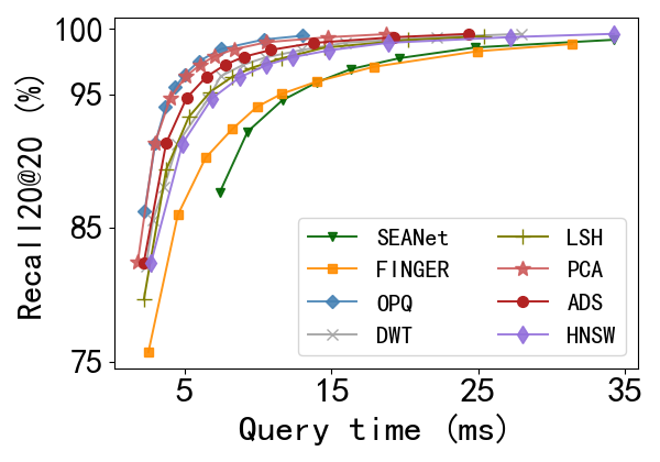
(a) GIST (D=960, LID=18.9)

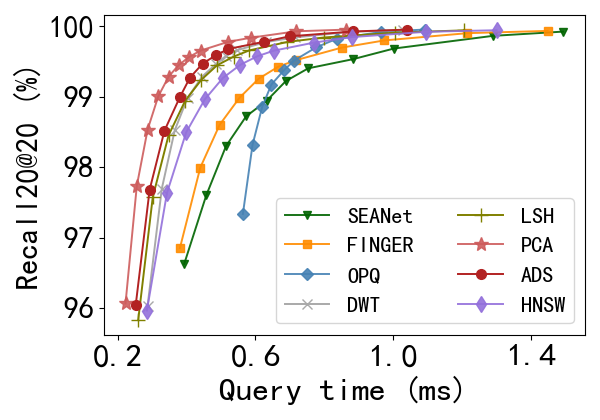
(b) MNIST (D=784, LID=6.5)

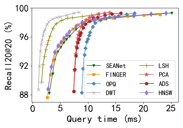
(c) Trevi (D=4096, LID=9.2)

Figure 1: ANNS performance on high D/LID datasets

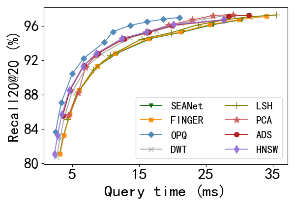
(a) Imagenet (D=150, LID=12)

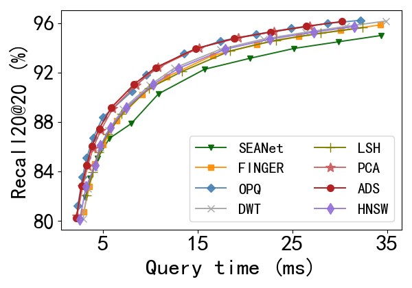
(b) Word2vec (D=300, LID=27)

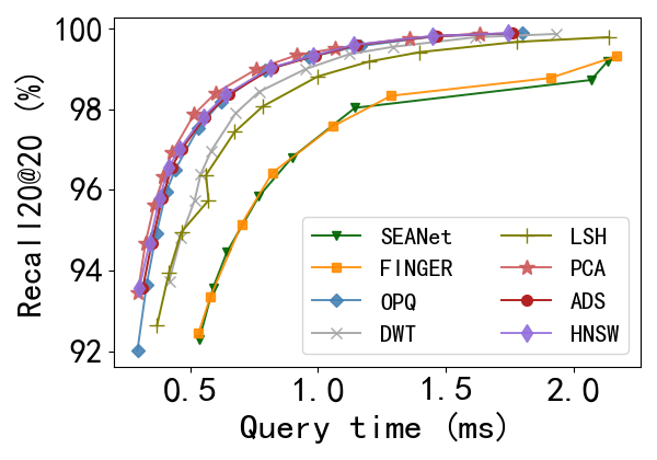
(c) Deep (D=96, LID=12)

Figure 2: ANNS performance on low D/LID datasets

5.2 Search Performance

Results summary

We benchmark DCOs on two groups of datasets with high and low $D/LID$, respectively. The first observation is that all DCOs do not always provide a performance gain compared with the original index, especially in low $D/LID$ datasets, matching the benefit threshold analyzed in Section 3. In summary, transformation-based DCOs, especially PCA and ADS are generally superior to others while OPQ achieves the best place on low-dimensional and hard datasets. And on high-dimensional and easy datasets, LSH and DWT are the optimal alternatives. We next investigate the reasons behind the benchmark results in the following w.r.t. the accuracy loss and efficient improvements respectively to analyze the results in-depth.

5.3 Accuracy Loss

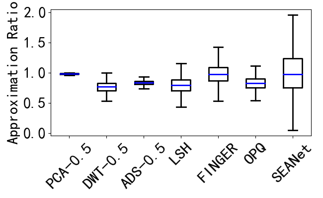
(a) All DCOs

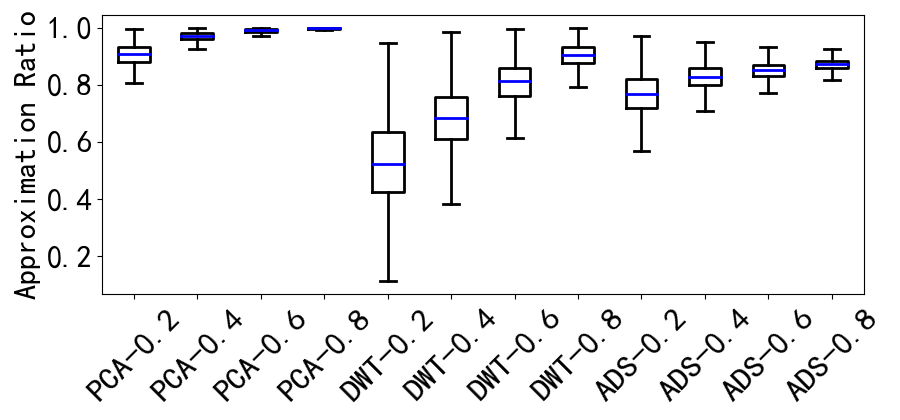
(b) Adaptive DCOs

Figure 3: Approximation ratio on GIST

We first sample partial vectors from training and test sets to evaluate the approximation ratios of different DCOs, defined as $AR=\frac{\widehat{dist}(v,q)}{dist(v,q)}$ where $\widehat{dist}$ is the estimated distance. Figure 3(a) depicts the distribution of $AR$ on GIST dataset, where PCA-0.5 means estimating distances by the first 50% dimensions on the transformed dataset. As lower-bounding techniques, $AR$ of PCA and DWT are surely below 1, while PCA is much tighter with a smaller variance. Similarly, although ADS does not provide a lower bound, it hardly generates false dismissals due to the reliable probabilistic guarantee. The tightness and variance of the approximated distance exactly reflect the final rankings of three transformation-based methods: PCA > ADS > DWT. The only exception is in ultra-high dimensional and easy datasets, where the pre-process time domains the low-recall range and the complexity of DWT $O(D)$ is superior to PCA and ADS $O(D^{2})$.

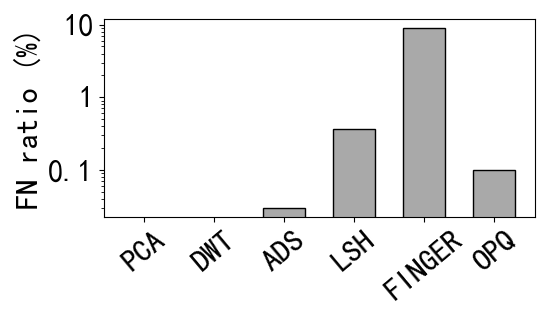
Figure 4: False negative ratio on GIST (recall=95%, k=500)

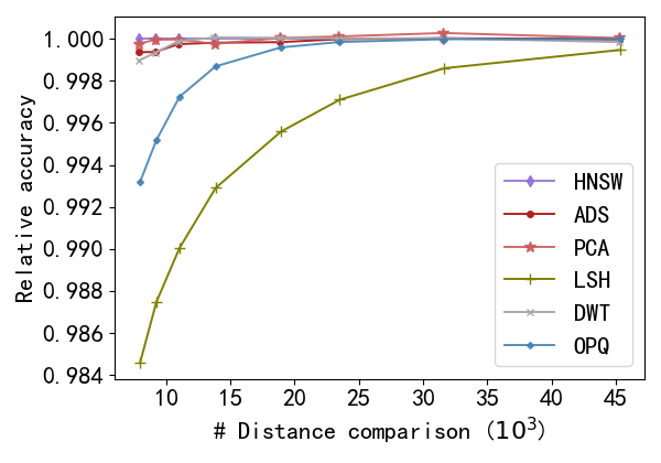
Figure 5: Accuracy loss on GIST (recall=95%, k=500)

At the same time, other categories of methods have larger variances of approximation ratios, especially for FINGER and SEANet. An interesting point is that the medians of these two are very close to 1.0, indicating that they serve as nice estimators of the actual distance. However, as shown in Figure 5, the false negative ratios of them, defined as $\frac{\#(\widehat{dist}(v,q)>dist(R_{ef},q)\geq dist(v,q))}{T}$ are exponentially higher than the others. The false negative samples describe the cases when a qualified neighbor point is wrongly pruned by DCOs, which is the root cause of DCOs’ accuracy loss. Note that OPQ and LSH more or less also suffer from this problem, i.e., relatively large variance of approximation ratios and ineligible false negative ratios. However, as shown in Figure 5, the accuracy loss becomes marginal as the number of distance comparisons increases, indicating that though some neighbors are wrongly pruned, the final destination area can still be reached from other routes with other neighbors by taking a long way around, and the actual $k$NN are hardly pruned. And in the final stage of searching, most efforts are devoted to ensuring the $k$NN found are actual [16], which does not improve the recall. In contrast, FINGER and SEANet are missing in Figure 5 for their large accuracy loss. It means that a large false negative ratio will make the ANNS lose the way (especially the key hops on the way) in the graph index and substantially delay the time to reach the destination area. Based on these analyses, we give our first insight: Tight and reliable lower-bound approximations benefit ANNS more than a general estimation of the actual distance.

5.4 Efficiency Improvements

We next explore the properties of different DCOs w.r.t. the efficiency improvement for ANNS. An important metric is the pruning ratio, as shown in Table 2. On GIST dataset, PCA and ADS are very efficient in pruning, benefiting from their adaptive dimension-level pruning and norm preservation during the transformation. That is, when the pruning fails, they can directly give the actual distance to give without completely computing it again. On low-dimensional or hard datasets, LSH is not competitive in terms of either accuracy loss or pruning ratio. FINGER though has a nice pruning ratio, the large false negative ratio substantially degrades the search efficiency. An interesting point is that although OPQ does not have a better pruning ratio nor accuracy loss than PCA and ADS, it achieves competitive overall performance. It is because the cost of evaluating the approximate distance in OPQ is smaller than PCA and ADS. Specifically, we only need to look up the distance table (memory access) and sum the results. And for PCA and ADS, we need to execute one time of multiplication and subtraction on each dimension with periodical comparison (even with a multiplier in ADS). As analyzed in Section 3, the cost of evaluating approximate distance is also a crucial factor.

Table 2: Pruning ratio on GIST ($k$=500, recall=95%)

Prune ratio (%)	PCA	DWT	ADS	LSH	FINGER	OPQ
Dim-level	63.6	20.6	38.5	22.4	54.6	34.1
Vec-level	93.2	93.2	93.1	28.6	61.9	34.9

5.5 SIMD compatibility

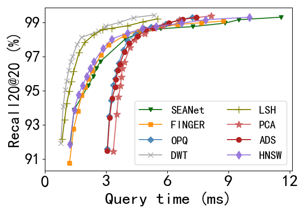
(a) Trevi (D=4096, LID=9.2)

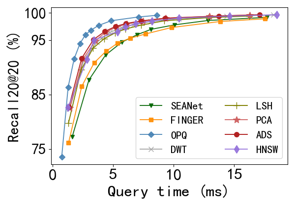
(b) GIST (D=960, LID=18.9)

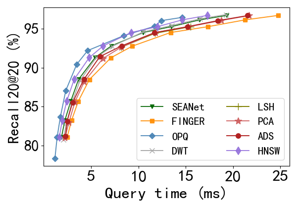
(c) Imagenet (D=150, LID=12)

Figure 6: ANNS performance with SIMD (AVX)

Figure 6 shows the performance of all DCOs and HNSW enhanced with SIMD techniques. It can be seen that the advantages of all DCOs compared with the original HNSW turn smaller. Specifically, only OPQ, PCA and ADS show benefit gains on GIST dataset while LSH and DWT remain superior on Trevi dataset. And in Imagenet, OPQ is the only one to provide benefit gains. The reason is that the raw distance calculations can fully enjoy the acceleration of SIMD while the approximate distance calculation, on the contrary, usually incurs extra computation overheads. For example, the transformation-based DCOs, adopt an adaptive pruning style which early abandons at the time when the pruning condition is satisfied. Thus, there is a trade-off between the pruning ratio and SIMD efficiency. When the data length (i.e. dimensionality) for vectorized execution is increased (e.g. from 4 to 16), we can use more efficient SIMD instructions while the pruning ratio is sacrificed. Therefore, the efficiency improvement is not as good as raw distance calculations. As geometry-based methods, FINGER relies more on memory access along with hamming distance calculations, so SIMD cannot help it in approximate distance calculations. As for LSH and DNN, since the projected distances are still in L2 format, it is easy to be optimized by SIMD. Additionally, SIMD optimizations for the approximate distance calculations of PQ-based DCOs, i.e., the look-up of distance table and a sum of the results from different segments, are well developed in the literature. Based on the results and analysis, we give our second finding: low-dimensional distance calculation or segment-level pruning tends to be more SIMD-friendly in approximate distance calculation.

6 Discussion and Conclusion

Open problems

Based on the investigation and insights from our benchmark, we provide several important open problems that are worth studying to further push the boundary of state-of-the-art.

1. As some classical methods like PQ perform competitively in most cases of our benchmark, it is meaningful to provide a theoretical accuracy guarantee, deterministic or probabilistic, for them to help find the Pareto curve.

2. Although deep neural networks currently do not perform well, there is still a large space to optimize by adjusting the loss functions or the network topology based on our insights.

3. It is promising to design DCOs natively combining the pruning techniques with SIMD instructions. For example, the features can be grouped in 256 bits and the approximate distance can be estimated between features in a SIMD-friendly way.

Limitations

Our benchmark can be extended in the following aspects to make it more extensive and comprehensive.

1. There are many optimizations and variants of the evaluated techniques such as PQ and LSH. It is interesting to figure out which kinds of optimizations can (be extended to) match our insights or improve query performance in a novel way.

2. On large datasets (e.g. billion-scale), some techniques evaluated in Fudist might meet scalability limitations. In that case, sampling might be a natural way to reduce the complexity while preserving the main features.

3. Although we only focus on DCOs that are orthogonal to specific ANNS indexes and search algorithms (except for FINGER), it is also interesting to see how current DCOs can be adapted to serve and optimize the specific search and indexing algorithm, as described in  [13, 28].

Conclusions

In this paper, we study the solutions of distance approximation and pruning served for ANNS. We first introduce classical techniques like PCA and DWT, and deep learning models like SEANet into this area. We further provide a detailed analysis of these methods along with the advanced techniques from recent research. To evaluate these methods fairly, we design a lightweight benchmark Fudist and conduct a comparative study on it. The analysis and insights obtained from the experimental results help researchers further understand the mechanisms of different techniques.

Appendix A Fudist Dataset Details

Trevi

Trevi is a collection of images of the Trevi Fountain in Rome, Italy, taken from Photo Tourism reconstructions . This dataset contains 100,000 image patches, each of which is sampled as $64\times 64$ grayscale with a canonical scale and orientation. The patch is flattened as a 4096-dimension vector. This dataset can be accessed at http://phototour.cs.washington.edu/patches/default.htm under no clear license.

MNIST

MNIST is a database of handwritten digits, which have been size-normalized and centered in a fixed-size image. The images were centered in a $28\times 28$ image by computing the center of mass of the pixels, and translating the image so as to position this point at the center of the $28\times 28$ field. Each vector is flattened as a 784-dimension vector. This dataset can be accessed at http://yann.lecun.com/exdb/mnist/ under the terms of the Creative Commons Attribution-Share Alike 3.0 license.

Cifar

Cifar is a labeled subset of 80 million tiny image dataset, consisting of $32\times 32$ color images in 10 classes, with 6,000 images per class. The images are represented by a 512-dimension GIST feature vector. This dataset can be accessed at https://www.cs.toronto.edu/~kriz/cifar.html under the terms of license CC BY 4.0.

Sun

Scene UNderstanding (SUN) database contains 397 categories and 79,106 images for scene recognition tasks. The images are represented by a 512-dimension GIST feature vector. This dataset can be accessed at https://vision.princeton.edu/projects/2010/SUN/ under the terms of the Creative Commons Attribution-Share Alike 4.0 license.

GIST

GIST dataset contains 1 million images represented by 960-dimension GIST descriptors. This dataset can be accessed at http://corpus-texmex.irisa.fr/ under no clear license.

Msong

Msong is a collection of one million western popular music pieces. This dataset comes with a set of features extracted by the API of The Echonest, which include tempo, loudness, timings of fade-in and fade-out, and MFCC-like features for a number of segments. This dataset can be accessed at http://www.ifs.tuwien.ac.at/mir/msd/ under the Open Access license.

Tiny

Tiny image dataset extracts 5 million images from 80 million images of size $32\times 32$ pixels collected from the Internet, crawling the words in WordNet. This dataset can be accessed at https://www.cse.cuhk.edu.hk/systems/hash/gqr/datasets.html under no clear license.

Nuswide

Nuswide is a web image dataset containing 268,643 images represented by 500-dimension bag of words based on SIFT descriptions. This dataset can be accessed at https://lms.comp.nus.edu.sg/wp-content/uploads/2019/research/nuswide/NUS-WIDE.html.

UKbench

UKbench contains 10200 images of N=2550 groups with each four images at size $640\times 480$. The images are rotated, blurred and have a tendency for computer science motives. This dataset can be accessed at https://archive.org/details/ukbench under no clear license.

Table 3: Dataset statistic

Datasets	Data size	Query size	D	LID	D/LID	Type
Trevi	99,900	200	4096	9.2	445.2	Image
MNIST	60,000	10,000	784	6.5	120.6	Image
Cifar	50,000	200	512	9.0	56.9	Image
Sun	79,106	200	512	9.9	51.7	Image
GIST	1,000,000	1,000	960	18.9	50.8	Image
Msong	994,185	1,000	420	9.5	44.2	Audio
Tiny	5,000,000	1,000	384	14.4	26.7	Image
Nuswide	268,643	200	500	24.5	20.4	Image
UKbench	1,097,907	200	128	7.2	17.8	Image
Crawl	1,989,995	10,000	300	15.7	19.1	Text
Notre	332,688	200	128	9.0	14.2	Image
SIFT	1,000,000	10,000	128	9.3	13.8	Image
Imagenet	2,340,373	200	150	11.6	12.9	Image
Word2Vec	1,000,000	1,000	300	26.6	11.3	Text
Deep	1,000,000	10,000	96	12.1	7.9	Image
Glove100	1,183,514	10,000	100	20.0	5.0	Text

Crawl

Crawl dataset provides a corpus for collaborative research, analysis and education. The text is converted to 300-dimension vectors with fastText. This dataset can be accessed at https://commoncrawl.org/ under the Open Access license.

Notre

Notre dataset contains about 0.3 million 128-d features of a set of Flickr images and a reconstruction from a collection of images from Notre Dame in Paris. This dataset can be accessed at http://phototour.cs.washington.edu/patches/default.htm under no clear license.

SIFT

SIFT dataset contains 1 million images represented by 128-dimension SIFT descriptors. This dataset can be accessed at http://corpus-texmex.irisa.fr/ under no clear license.

Imagenet

Imagenet is a large visual database designed for use in visual object recognition software research. It contains about 2.4 million data points with 150 dimensions of dense SIFT features. This dataset can be accessed at https://www.image-net.org/ under no clear license.

Word2vec

Word2vec dataset is sampled from the word2vec embeddings which are trained on part of Google News dataset. This dataset can be accessed at https://code.google.com/archive/p/word2vec/ under the license of Apache License 2.0.

Deep

Deep vectors are produced as the outputs from the last fully-connected layer of the GoogLeNet model, which was pretrained on the Imagenet classification task. The embeddings are then compressed by PCA to 96 dimensions and L2-normalized. This dataset can be accessed at http://sites.skoltech.ru/compvision/noimi under no clear license.

Glove100

Glove (Global Vectors for Word Representation) is a word vector dataset produced by the corresponding Glove unsupervised learning algorithm. This dataset is the pre-trained word vectors from Wikipedia 2014  and Gigaword 5  corpus. This dataset can be accessed at https://nlp.stanford.edu/projects/glove/ under the Public Domain Dedication and License v1.0.

Appendix B Explanation and Analyses of Theoretical Results

We now prove and explain the benefit thresholds described in Table 1 in detail. Since the exhaustive computation cost of all distance comparisons is $T\cdot\mathcal{O}(D)$, where $T$ is the total times of distance comparisons and $\mathcal{O}(D)$ is the complexity to compute Euclidean distance between two vectors, the actual cost for DCOs should be less than this exhaustive cost so that users can gain the overall benefit. The actual cost consists of three parts, the preprocess cost, the approximation cost (i.e., the pruning cost), and the cost to compute the full distance for the vectors not pruned. Note that the preprocess cost here only refers to the cost of transforming a query to a certain format (e.g., rotated by a prepared matrix, quantized by a codebook and etc), and we only use a constant $C$ to represent it since it is usually small and can be amortized by the further distance comparisons. More detailed analyses of preprocess cost are elaborated in Appendix C.

Now we focus on the approximation cost and the distance calculation cost. For transformation-based DCOs, the approximation cost for a vector is not fixed, ranging from $\mathcal{O}(1)$ to $\mathcal{O}(D)$, depending on which point the approximated distance exceeds the threshold. We thus use the cost to evaluate one dimension $f_{d}$, and the dimension-level pruning ratio $p_{d}=1-\frac{\#dim.calc.}{D\cdot T}$ to describe the approximation cost, i.e., $T\cdot D\cdot f_{d}\cdot(1-p_{d})$. And since transformation-based DCOs can naturally obtain the actual distance when the pruning fails, no distance calculation cost exists. Then we can get Equation 1 for transformation-based DCOs, and the final benefit threshold can be easily deduced from Equation 1 by the basic laws of inequalities.

For DCOs of other types, we assume the approximation cost for a whole vector is $f_{v}$ which is asymptotically smaller than $\mathcal{O}(D)$, and the vector-level pruning ratio $p_{v}=1-\frac{\#full\,dist.calc.}{T}$. Then the total approximation cost is $T\cdot f_{v}$ and the full distance cost is $T\cdot(1-p_{v})\cdot O(D)$. By summarizing these two terms and the preprocess cost $C$, we can get the real cost for these DCOs as shown in Equation 2, and the benefit threshold in Table 1, finally.

We next analyze the impacting factors in the benefit thresholds.

• $p_{d}$. The value range of $p_{d}$ for transformation-based DCOs is $(0,1]$, whereas for other DCOs $p_{d}$ can be a negative number and the limit depends on the ways of approximation. It is because the approximation is an additional cost for non-transformation DCOs. Considering the extreme case when all the pruning test fails, the actual cost is the exhausted computation cost plus the pruning cost.

• $p_{v}$. In contrast to $p_{d}$, $p_{v}$ is always non-negative, belonging to $[0,1]$. And usually for transformation-based DCOs, $p_{v}$ is very close to $1$.

• $f_{d}$. $f_{d}$ is usually larger than the amortized cost of computing Euclidean distance on one dimension due to the additional cost of evaluating the pruning criteria. For example, ADS needs to multiply the approximated distance and compare it with the threshold. Therefore, transformation-based DCOs often evaluate the pruning criteria after computing a period of dimensions to amortize the cost (described in Appendix C.2).

• $f_{v}$. The exact cost of $f_{v}$ varies across different DCOs, but all below $\mathcal{O}(D)$. Details will be elaborated in Appendix C.2.

• $C$. It is clear that in the benefit thresholds of all DCOs, the terms containing $C$ tend to be zero when $T$ is a large value. However, in some easy datasets (e.g., Trevi), a large $T$ is unnecessary to find the $k$NN. On the other, $C$ is often also $\mathcal{O}(D)$ with a large multiplier. In such cases, these terms should not be ignored.

Appendix C Analyses of Extra Costs of DCOs

Table 4: Extra costs of DCOs

Category	DCO	Index time cost	Memory cost (4 bytes)
Transformation	PCA	$\mathcal{O}(n^{2}D+ND^{2})$ 1	$D^{2}$
	DWT	$\mathcal{O}(ND)$	$0$
	ADS	$\mathcal{O}(ND^{2})$	$D^{2}$
Projection	LSH	$\mathcal{O}(NDd)$ 2	$Nd+Dd$
	SEANet	$\mathcal{O}(nX)$ 3	$\mathcal{O}(X)$
Quantization	OPQ	$\mathcal{O}(t_{1}n^{2}D+(t_{1}n+t_{2}n+N)DK_{s}))$	$Nm+DK_{s}+D^{2}$
Geometry	FINGER	$O(\left|E\right|D^{2}+ND^{2}+\left|E\right|Dd+NDd)$ 4	$(2+\frac{d}{32})\left|E\right|+(1+d)N$

• $n$ is the size of training set, and $N$ is the size of dataset.

• $d$ is the dimensionality of projected vectors (e.g., the number of hash functions).

• $X$ depends on the number of parameters.

• $\left|E\right|$ is the number of edges in the graph index, and $d$ is the number of LSH hash functions.

The extra costs of DCOs include the additional indexing time cost and memory cost (listed in Table 4), as well as query time cost (listed in Table 5).

In the indexing stage, DCOs need to compute auxiliary information that will be used in the query stage to help speed up distance calculation. Usually, we sample randomly a portion of data from the dataset as the training set. In the analyses below, we assume the cardinality of the dataset and the training set is $N$ and $n$, respectively.

In the querying stage, the auxiliary information will be loaded into memory and thus produces extra memory cost. When a query vector comes, it usually needs to be preprocessed into other formats (e.g., rotated by an orthogonal matrix, projected by a group of hash functions, embedded by neural networks, etc.). The time cost of preprocess forms the factor $C$ in the benefit thresholds. It though is often insignificant due to the amortization by a large number of distance calculations, determines the total time in some cases as explained in Appendix B. We also analyze the approximation costs for different DCOs, which is the most important property determining the query performance. We only show the asymptotic complexity of evaluating one dimension for transformation-based DCOs and the whole vector for other types of DCOs in Table 4 respectively. Details will be elaborated in Appendix C.2.

Finally, we discuss other limitations when adopting DCOs in ANNS index in different scenarios and provide suggestions for these users.

C.1 Indexing Time and Memory Cost

The indexing time cost comes from the calculations of the auxiliary information. This information is index-independent (except FINGER) and can be prepared once the data is ready. It is a little different for transformation-based DCOs that build the index on the transformed vectors and thus the auxiliary information must be obtained before building the index. The original vectors (before transformation) can be directly discarded since it is usually meaningless and users usually only care about the identifiers of $k$NN. To say the least, the original vectors can still be restored by inverse transformation (i.e., multiply the inverse of the transformation matrix), which is not time costly.

Recall that all transformation-based DCOs preserve the norm during the transformation (i.e., the distance between vectors keep unchanged) and the ANNS index is built relying on only the distance between vectors. So the index built after transformation is the same as before in theory (i.e., neglect the errors in float point number calculations). Therefore, the comparison between transformation-based DCOs and other types of DCOs is still fair.

Another choice for transformation-based DCOs is to build the index on the original vectors and store the transformed vectors in separate data structures along with the transformation matrix. However, it will double the memory consumption and introduce more memory accesses, which are unnecessary in real applications.

PCA

The time complexity of PCA is $\mathcal{O}(n^{2}D)$ and we need to store the matrix consisting of eigenvectors (ordered by the corresponding eigenvalues from the highest to the lowest), which is a $D\times D$ orthogonal full-rank matrix, occupying $D^{2}$ elements of space. After that, we need to rotate the dataset with the matrix, with time complexity $O(ND^{2})$.

DWT

In contrast to PCA, DWT transforms each vector independently without the need of learning a rotation matrix from a training set. And the transformation is very efficient with $O(D)$ linear complexity and no other auxiliary information. As a result, DWT is the most lightweight DCO in our benchmark.

ADS

ADS is also independent of data distribution. It generates a random transformation matrix ($D\times D$) and all vectors are rotated by this matrix. So the time complexity is $\mathcal{O}(ND^{2})$ and the memory cost is $D^{2}$ elements of space, the same as PCA.

LSH

Similar to ADS, LSH generates $d$ hash functions in the format of inner product, where each function consists of $D$ parameters to align with the dimensionality of the vectors. All parameters in the hash functions are sampled from the Gaussian distribution. Therefore, the projection of the dataset can be performed by matrix multiplication, with $\mathcal{O}(NDd)$ time complexity, and we only need to store the parameters of the hash functions, occupying $Dd$ elements of space.

SEANet

The extra indexing cost for SEANet is to train the CNN model with the training set. It depends on the number of epochs and the training complexity of the model. The time complexity of training is linearly related to the dimensions of the vector. And the memory cost is in direct proportion to the number of parameters.

OPQ

OPQ trains a codebook with the training set by k-means clustering on each subspace, and encodes the dataset as codewords. Thus the memory consumption includes three parts, the codebook, the rotation matrix and the codewords. The codebook contains $m$ subspaces and on each subspace we have $K_{s}$ clustering centroids which are also vectors of dimensionality $D/m$. Thus, the codebook contains $mK_{s}D/m=DK_{s}$ elements. Similar to PCA and ADS, the rotation matrix covers $D^{2}$ elements of space. As for the codewords, for each vector, OPQ cuts it into $m$ equal-length segments and represents the subvector on each space with the identifier of clustering centroid. Strictly speaking, $K_{s}$ centroids need identifiers of only $logK_{s}$ bits. Here to keep the table concise, we use one 4-byte integer as the identifier, which can support up to $2^{32}>4$ billion centroids. Therefore, the codewords occupy $Nm$ elements of space.

Next, we introduce the time complexity of training OPQ. OPQ tries to find the optimal rotation matrix and the optimal clustering centroids by minimizing the distortion error. In each iteration, OPQ first fixes the rotation matrix and optimizes the clustering by adjusting the centroids like k-means. Then OPQ fixes the centroids and optimizes the rotation matrix. Due to the NP-hard complexity of this optimization problem, OPQ approximates it by first encoding the training vectors with the current codebook and then applying Singular Value Decomposition (SVD) to the multiplication of the original training set matrix and the encoded codewords matrix. Then the multiplication of the left and right singular vector matrices is regarded as the rotation matrix. The complexity of training clustering centroids and matrix multiplication in one iteration is $O(nDK_{s})$ and $O(n^{2}D)$, respectively. This process ends until the maximum number of iterations $t_{1}$ is reached. The next round fixes the rotation matrix and updates the clustering centroids with $t_{2}$ iterations.

FINGER

The auxiliary information of FINGER is prepared after the graph index is built. Specifically, we need to compute the$||d_{proj}||$ and $||d_{res}||$ for each edge and $||c||$ for each node in the graph index, which costs the $O(\left|E\right|D^{2}+ND^{2})$ time. Besides, FINGER pre-computes the sigend LSH of $d_{res}$ for each edge and rotated vectors of $c$ with time complexity $O(\left|E\right|Dd+NDd)$. The symbols above are consistent with the original paper.

C.2 Query Time Cost

Table 5: Extra query costs of DCOs

Category	DCO	Preprocess ($C$)	Approximation ($f_{d}$/$f_{v}$)
Transformation	PCA	$\mathcal{O}(D^{2})$	$\mathcal{O}(1/\Delta D)$ 1
	DWT	$\mathcal{O}(D)$	$\mathcal{O}(1/\Delta D)$
	ADS	$\mathcal{O}(D^{2})$	$\mathcal{O}(2/\Delta D)$
Projection	LSH	$\mathcal{O}(Dd)$2	$\mathcal{O}(d)$
	SEANet	$\mathcal{O}(DX^{\prime})$3	$\mathcal{O}(d)$
Quantization	OPQ	$\mathcal{O}(DK_{s})$4	$\mathcal{O}(m){\textsuperscript{5}}$
Geometry	FINGER	$\mathcal{O}(Dd)$	$\mathcal{O}(log(d)+C)$6

• $\Delta D$ is the number of computed dimensions before evaluating the pruning criteria in each iteration.

• $d$ is the dimensionality of projected vectors (e.g., the number of hash functions).

• $X^{\prime}$ depends on the model topology and the number of parameters.

• $K_{s}$ is the number of clustering centroids.

• $m$ is the number of segments.

• $C$ is the time cost to read and sum pre-computed information.

The additional query time cost comes from the transformation of the query vector and the approximate distance calculation. For transformation-based DCOs, evaluating the pruning criteria on each dimension is too expensive so we usually set a user-defined hyper-parameter $\Delta D$ to control the evaluation frequency. Note that for transformation-based DCOs we use the dimension-level cost $f_{d}$ to represent the approximation cost while for others we use the vector-level cost $f_{v}$.

PCA

The preprocess time cost of PCA is $O(D^{2})$ due to the matrix multiplication. In approximate distance calculation, we evaluate the pruning criteria for every $\Delta D$ dimensions. Thus the amortized additional cost for evaluating each dimension is $\mathcal{O}(1/\Delta D)$.

DWT

DWT transformation of a query vector is $O(D)$ time complexity. And the extra approximation cost is also $\mathcal{O}(1/\Delta D)$.

ADS

Like PCA, ADS transformation is also $O(D^{2})$ for matrix multiplication. In approximation, ADS needs to multiply a coefficient on the partial distance to evaluate the pruning criteria. Therefore the extra amortized cost is $\mathcal{O}(2/\Delta D)$.

LSH

LSH also applies matrix multiplication on the query vector but the size of the matrix is $D\times d$. And the approximate distance is defined as the L2 distance between the transformed vectors, with $\mathcal{O}(d)$ time complexity.

SEANet

The preprocess of a query vector is one time of inference and the time complexity depends on the number of parameters. The approximate distance calculations are the L2 distance between two embedding vectors, with $\mathcal{O}(d)$ time complexity.

OPQ

OPQ needs to prepare a distance table before probing the index. The time cost is the same as encoding a vector $\mathcal{O}(DK_{s})$. And when computing the approximate distance, OPQ only needs to look up the distance table $m$ times and sum the results. Compared with the format of L2 distance calculation, OPQ does not involve any multiplication operations.

FINGER

FINGER requires projecting the query with LSH rotation matrix with time complexity $\mathcal{O}(Dd)$. The major procedure of computing approximate distance is to estimate the inner product value of two vectors, which is facilitated by the humming distance between two binary vectors. We use the built-in instruction of GCC to speed up the humming distance calculation with only $\mathcal{O}(log(d))$ time complexity. Besides that, we also need to load some other numbers from the pre-computed auxiliary information with constant time complexity.

C.3 Discussion

Given the detailed analysis of all the DCOs included in our benchmark, we now provide a comparative study and a rank. In terms of extra indexing time, DWT is the fastest, and the next LSH and ADS are also very fast. PCA, OPQ and SEANet are slower and they rely on the size of the training set and the last two also rely on the number of iterations/epochs. FINGER introduces the largest cost since it needs to check each edge.

As for the memory cost, DWT does not need any extra memory while PCA and ADS only incur a little cost. LSH and OPQ store encoded (and compressed) vectors which are usually several times smaller than the original dataset. The memory cost of SEANet is the size of the model whereas FINGER introduces the largest memory cost due to the large number of edges.

In terms of the extra query cost, DWT is also the fastest w.r.t. the preprocess cost while LSH and FINGER are the next. The preprocess cost of PCA and ADS should not be neglected on easy and high-dimensional datasets. While the costs of OPQ and SEANet depend on the number of clustering centroids and the number of model parameters, respectively.

Sampling

Note that PCA, OPQ and SEANet need to sample from the dataset to construct the training set. If the training set is not a proper representative of the original data distribution, it will degrade the effectiveness of the transformation or projection. Therefore, how to sample representative data from the dataset is also an important problem for these DCOs.

Streaming ANNS

Another cost of these DCOs is in the insertion or update operation, where the update can be viewed as the composition of insertion and deletion. For example, PCA, ADS and LSH need to transform the new vector with a rotation matrix, while OPQ needs to encode it with the codebook and SEANet embeds it with neural networks. The cost of these operations is the same as the query preprocess cost. The only exception is FINGER, which needs to additionally maintain auxiliary information with the neighborhood and thus the extra insertion cost is large.

Appendix D Experimental Details

D.1 Adaption of Baseline Methods

We now describe how to adapt the techniques mentioned in our benchmarks to be DCOs. Since the approximate distances of PCA and DWT are always the lower bound of actual distance, we can check whether the approximate distance is larger than the pruning threshold (i.e., $dist(R_{ef},q)$), and if so (i.e., $dist(v,q)\geq\widehat{dist}(v,q)>R_{ef}>dist(R_{ef},q)$), the current neighbor can be simply skipped.

On the contrary, for LSH, OPQ and SEANet, we add a scale factor $\alpha$ when evaluating the pruning condition. That is, we change the distance comparison from $\widehat{dist}(v,q)>dist(R_{ef},q)$ into $\widehat{dist}(v,q)>\alpha\cdot dist(R_{ef},q)$. The larger $\alpha$ is, the smaller the probability of pruning is. In other words, larger $alpha$ trades efficiency for accuracy. For DCOs prone to produce false dismissals, we enlarge $alpha$ to ensure accuracy. Note that for FINGER we also add $alpha$ to reduce accuracy loss although it is not designed by the original paper.

SIMD support

We adopt the SIMD implementation in hnswlib for Euclidean distance calculation. For approximate distance calculation, only OPQ has the SIMD version and we adopt the implementation in FAISS. Since the format of approximated distance calculation of other DCOs except for FINGER is also the Euclidean distance, we implement the SIMD version in the same way as full distance calculation. But note that a short vector can not yet leverage the full power of SIMD optimizations due to the limited parallelism. For transformation-based DCOs, we set the parallelism of the SIMD instructions to be equal to $\Delta D$ to reconcile the pruning ratio with the acceleration of vectorized execution.

D.2 Reproduce Procedures

Sampling

Since in Fudist benchmark, the sizes of datasets are all million-level, we regard the whole dataset as the training set for OPQ and PCA. And we assume the dataset and the query set are from the same distribution as they usually originate from the same embedding model, so there is no problem of over-fitting. For SEANet, we randomly sample 50000 vectors for training the model to ensure efficiency.

Dimensionality aligning

DWT requires the length of the vector to be a power of two while OPQ requires it to be a multiple of the number of segments. For these two DCOs, we add padding zeros into the dataset whose dimensionality cannot satisfy the requirements. And for DWT, we remove the all-zero columns after transformation.

Workflow

To reproduce our benchmark results, users need to prepare the dataset in the correct format, build the base ANNS index and prepare auxiliary information (before or after the indexing), and finally execute queries. In the querying stage, Fudist loads the corresponding auxiliary information according to the name of DCO provided by the user and preprocesses the query vector. Also, the distance comparison operation is replaced by the interface provided by Fudist.

Reported results

Every reported result is the mean value of 3 runs of the same experiment. The query time is the average of all the queries in the query set. We omit the error bars since the variations are all within 5%.

Measure

We measure the search accuracy with recall. Given the set of approximate search results $A$ containing $k$ vectors, and the set of ground truth $GT$ also containing $k$ vectors, recall is defined as

$$recall\,k@k=\frac{|A\cap GT|}{k}$$ (3)

Extended to more ANNS indexes

Fudist can be extended to more ANNS indexes. The only work is to add a preprocess step before querying, and replace the distance comparison with Fudist DCO interface.

D.3 Hyper-parameters

We use grid search to select the optimum combinations of hyper-parameters. The graph index is first fixed and then we select hyper-parameters for DCOs.

Table 6: Optimal hyper-parameters

	HNSW	OPQ	LSH	FINGER
Trevi	$M$=16	$m$=8, $\alpha$=1.0	$d$=64, $p_{\tau}=0.8$	$\alpha$=1.6
MNIST	$M$=8	$m$=8, $\alpha$=0.9	$d$=64, $p_{\tau}$=0.95	$\alpha$=1.8
Cifar	$M$=8	$m$=8, $\alpha$=0.95	$d$=64, $p_{\tau}$=0.95	$\alpha$=3.0
Sun	$M$=8	$m$=8, $\alpha$=0.9	$d$=64, $p_{\tau}$=0.95	$\alpha$=3.0
GIST	$M$=16	$m$=8, $\alpha$=0.8	$d$=64, $p_{\tau}$=0.8	$\alpha$=1.5
Msong	$M$=8	$m$=6, $\alpha$=0.98	$d$=64, $p_{\tau}$=0.98	$\alpha$=1.2
Tiny	$M$=48	$m$=8, $\alpha$=0.9	$d$=16, $p_{\tau}$=0.99	$\alpha$=1.6
Nuswide	$M$=48	$m$=10, $\alpha$=0.8	$d$=64, $p_{\tau}$=0.99	$\alpha$=1.5
UKbench	$M$=16	$m$=8, $\alpha$=1.2	$d$=16, $p_{\tau}$=0.99	$\alpha$=1.5
Crawl	$M$=16	$m$=6, $\alpha$=0.95	$d$=16, $p_{\tau}$=0.99	$\alpha$=1.5
Notre	$M$=8	$m$=8, $\alpha$=1.0	$d$=16, $p_{\tau}$=0.99	$\alpha$=1.8
SIFT	$M$=16	$m$=8, $\alpha$=0.98	$d$=16, $p_{\tau}$=0.99	$\alpha$=1.8
Imagenet	$M$=16	$m$=6, $\alpha$=0.95	$d$=16 $p_{\tau}$=1.0	$\alpha$=1.5
Word2Vec	$M$=48	$m$=6, $\alpha$=1.0	$d$=16, $p_{\tau}$=0.95	$\alpha$=1.5
Deep	$M$=16	$m$=8, $\alpha$=1.1	$d$=16, $p_{\tau}$=0.95	$\alpha$=1.6
Glove100	$M$=16	$m$=4, $\alpha$=1.0	$d$=16, $p_{\tau}$=0.99	$\alpha$=1.8

Base graph index

We select HNSW as the base graph index, implemented by hnswlib. For the base graph index, we fix the parameter $efConstrution$ to be 500 as recommended . The parameter $M$ that controls the maximum out-degree of a node in the graph is adjusted to obtain the smallest value while achieving the optimum efficiency-accuracy trade-off, as shown in Table 6.

Transformation-based DCOs

For transformation-based DCOs, we fix $\Delta D$ to be 32 as it almost always achieves the best performance except for very hard datasets, where the pruning ratio cannot reach the benefit threshold and thus the evaluations of pruning criteria are a burden. It is not practical for actual cases to adjust $\Delta D$ to be a very large value on these datasets. And for ADS, we fix the hyper-parameter $\epsilon_{0}$ to be 2.1 as recommended, which usually reaches the optimum in our experiments.

LSH

LSH have two hyper-parameters $p_{\tau}$ and $d$. The former represents the confidence level and a larger $p_{\tau}$ trades efficiency for accuracy. $d$ is the number of hash functions and also the dimensionality of projected vectors.

SEANet

SEANet requires multiple hyper-parameters for model training in the indexing stage, and 1 scaling factor in the querying stage. We set the size of the sampling dataset as 50000 and an appropriate number of epochs that allow convergence. Other hyper-parameters are set as default values in the original paper.

OPQ

OPQ has 4 hyper-parameters in the indexing stage and 1 scaling factor in the querying stage. $m$ is the number of segments and $K_{s}$ is the number of clustering centroids which is fixed to be 256 as recommended. The maximum numbers of the first iterations $t_{1}$ and the second iterations $t_{2}$ are both fixed to 20. We assume to execute one round for clustering in the first iteration by default.

FINGER

in the indexing stage, FINGER’s hyper-parameters include $d$, the number of LSH hash functions and $n$, the sampling number of $d_{res}$ vectors for learning the eigenvectors to optimize the LSH rotation matrix. And it needs a scale factor $\alpha$ in the query stage. In our experiments, we fix $d$ to be 64 as recommended.

Appendix E Additional Experimental Results

We now report the complete benchmark results of ANNS performance, with and without SIMD optimizations, and also the approximation ratios on the 16 real datasets for all DCOs .

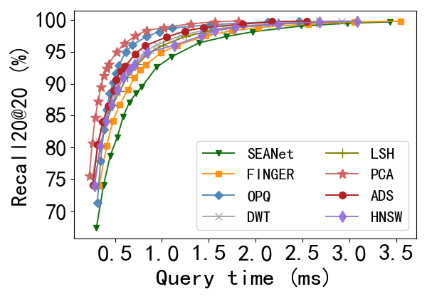
(a) Cifar

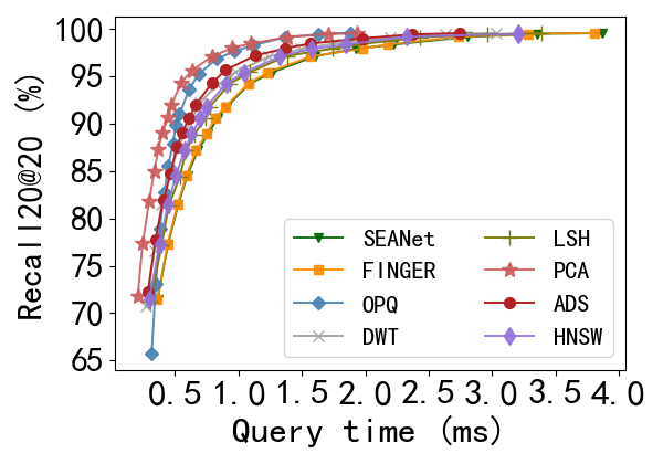
(b) Sun

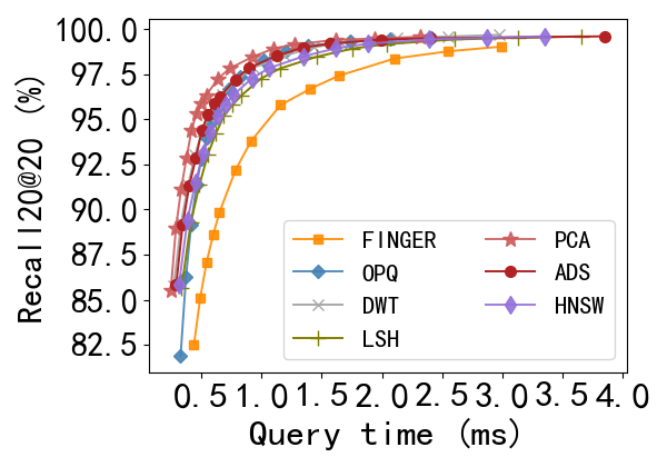
(c) Msong

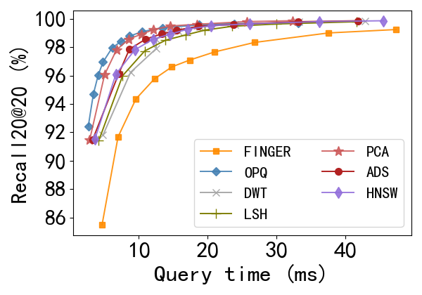
(d) Tiny

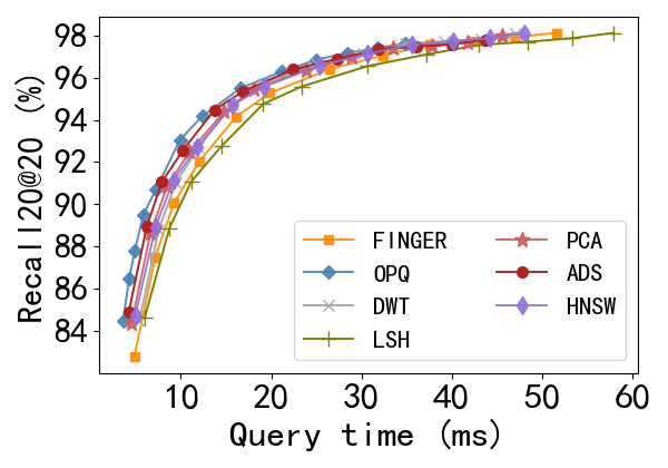
(e) Nuswide

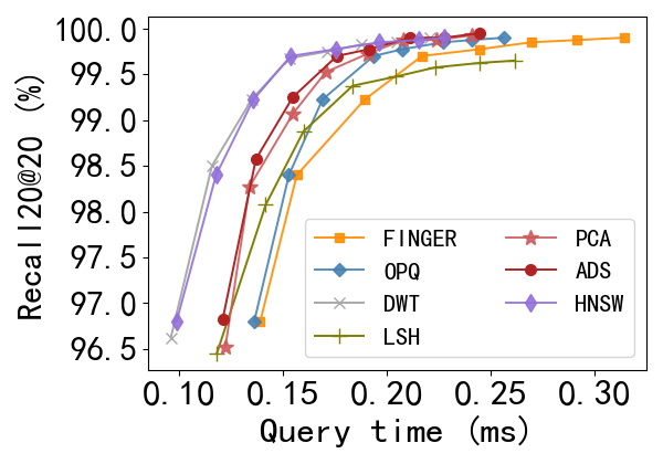
(f) UKbench

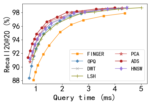
(g) Crawl

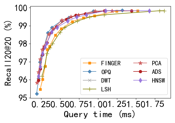
(h) Notre

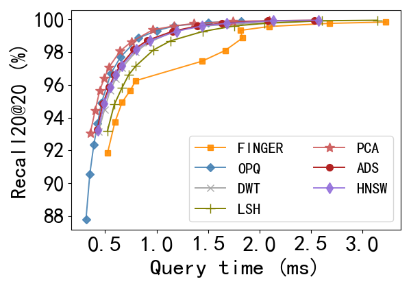
(i) SIFT

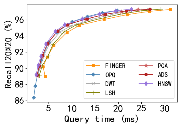
(j) Glove100

Figure 7: ANNS performance

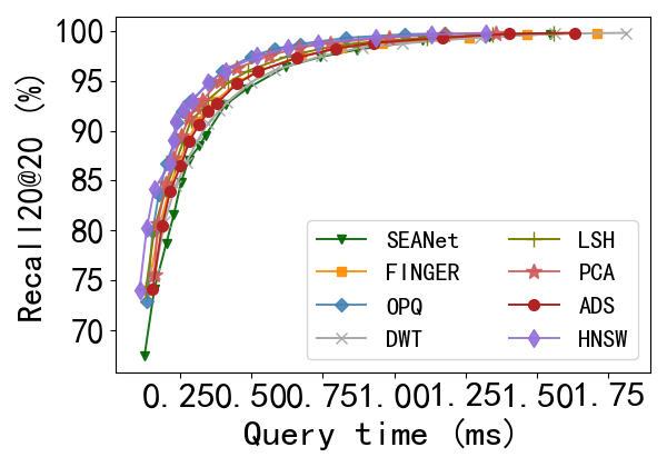
(a) Cifar

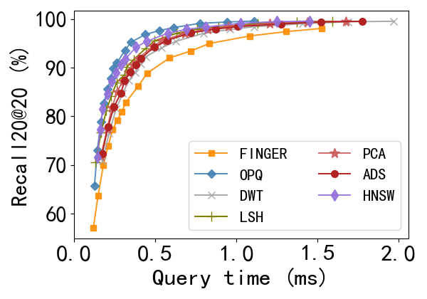
(b) Sun

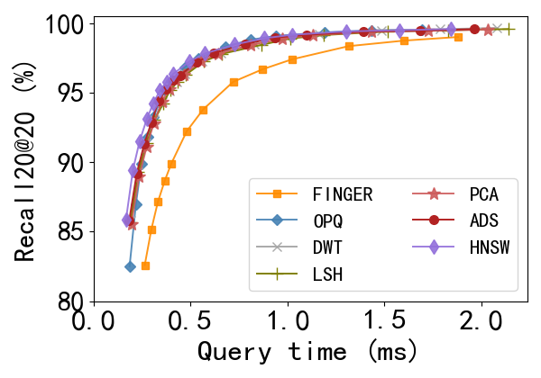
(c) Msong

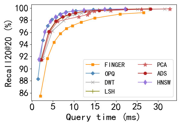
(d) Tiny

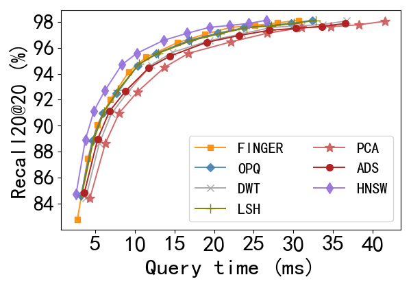
(e) Nuswide

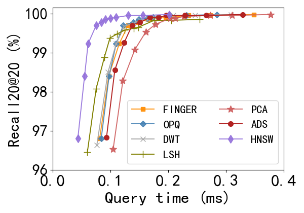
(f) UKbench

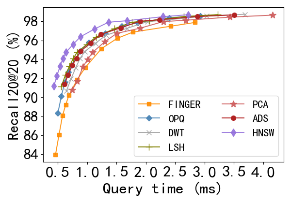
(g) Crawl

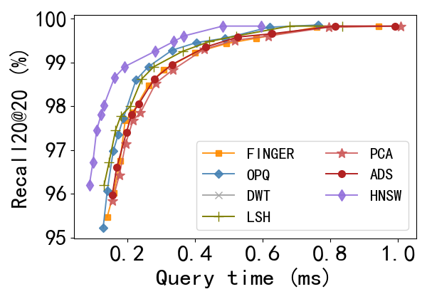
(h) Notre

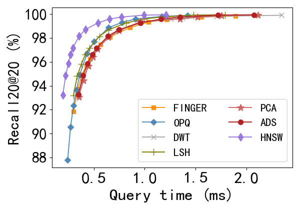
(i) SIFT

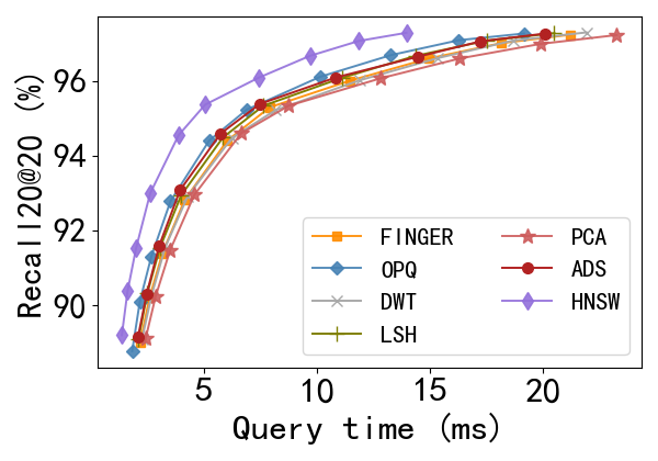
(j) Glove100

Figure 8: ANNS performance with SIMD

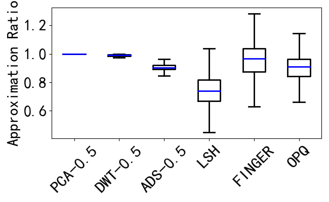
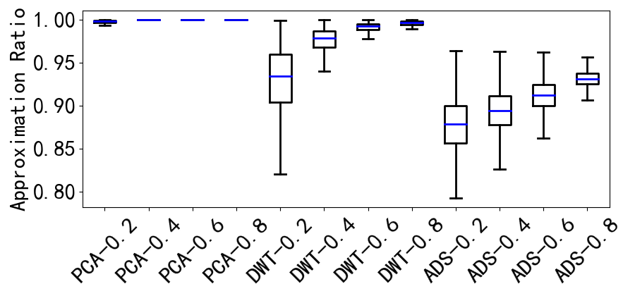
(a) Trevi

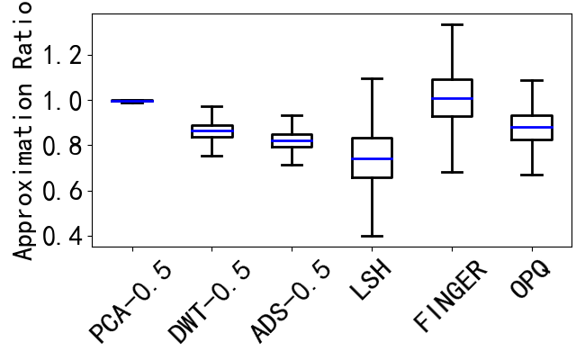
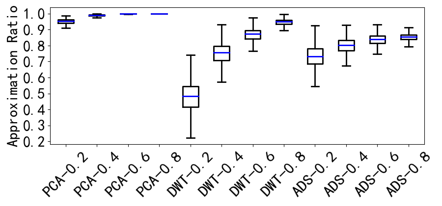
(b) MNIST

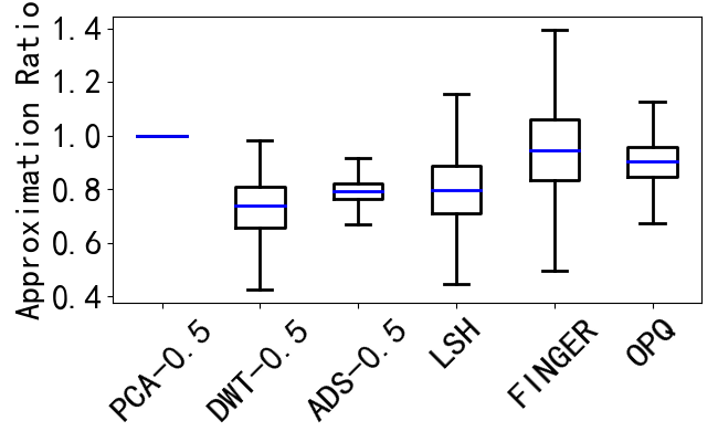
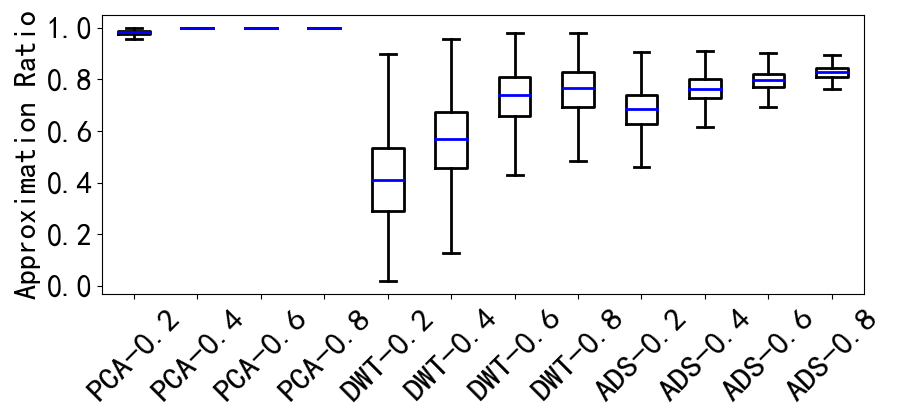
(c) Cifar

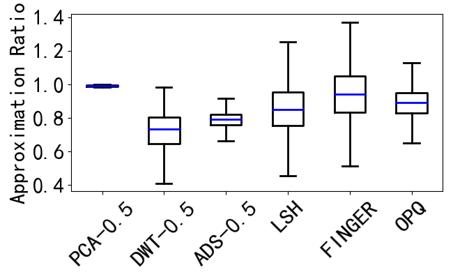
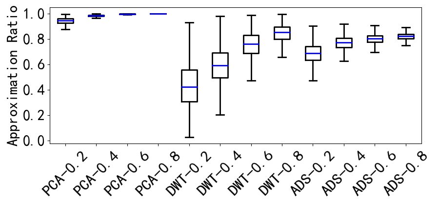
(d) Sun

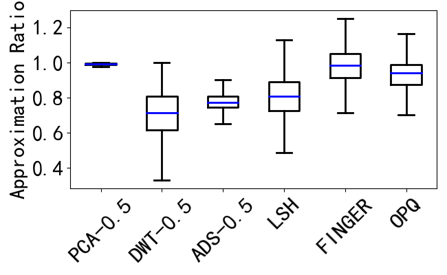
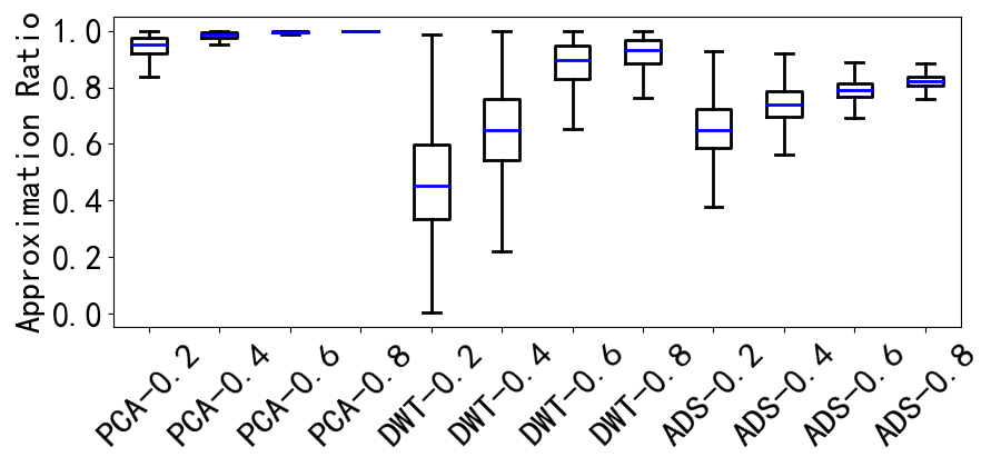
(e) Mson

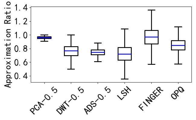
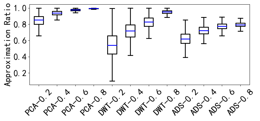
(f) Tiny

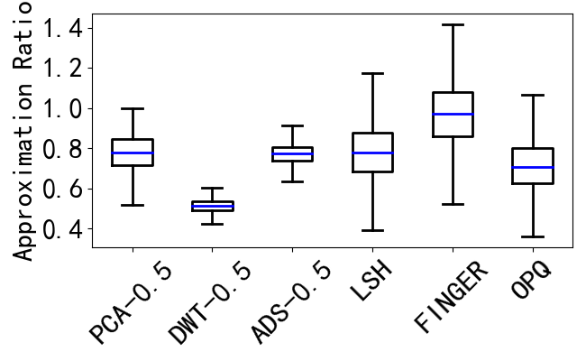
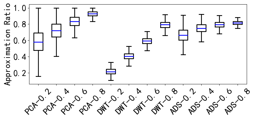
(g) Nuswide

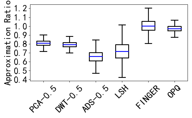
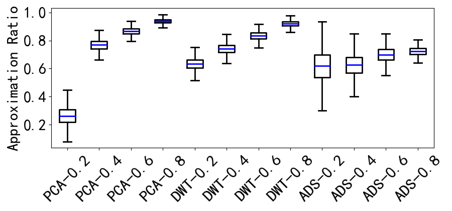
(h) UKbench

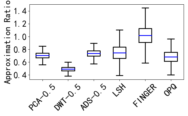
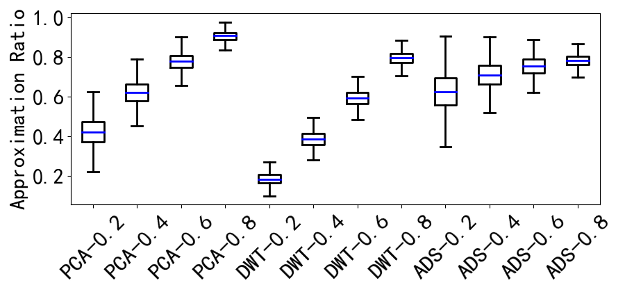
(i) Crawl

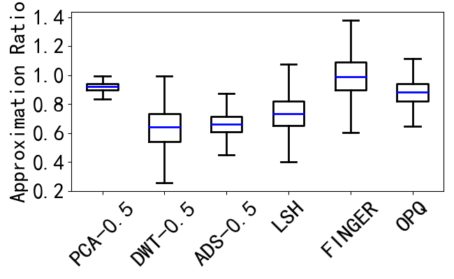
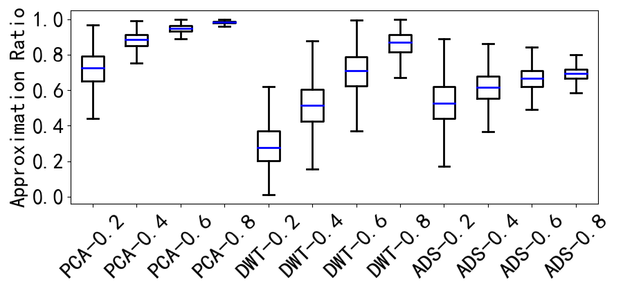
(j) Notre

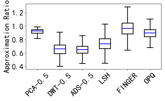
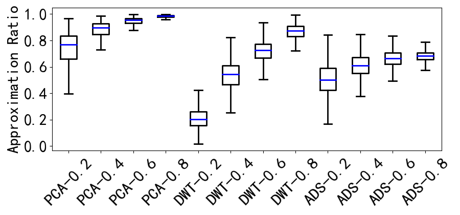
(k) SIFT

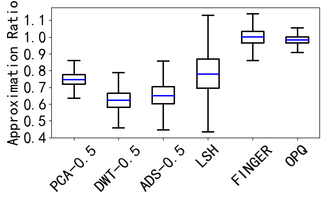
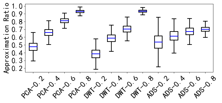
(l) Imagenet

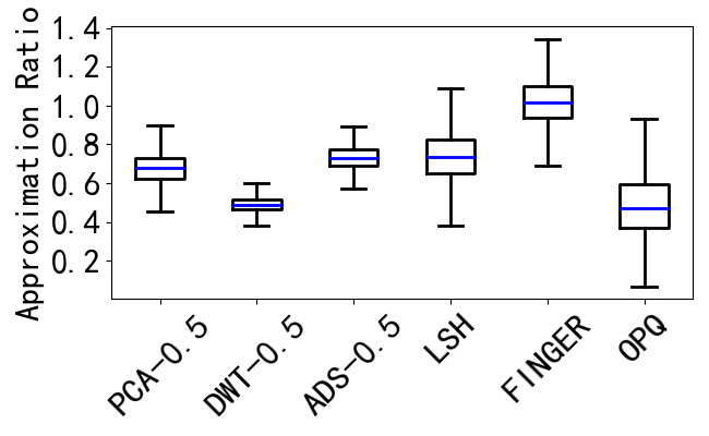
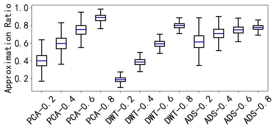
(m) Word2Vec

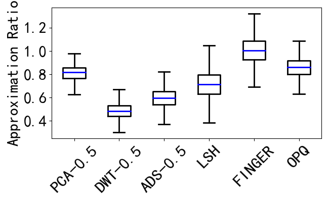
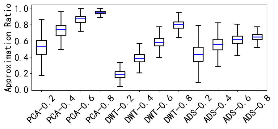
(n) Deep

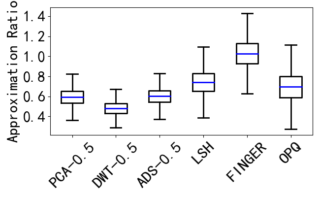
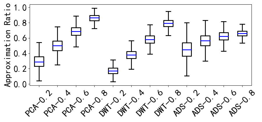
(o) Glove100

Figure 9: Approximation ratio

References

- [1] Hervé Abdi and Lynne J. Williams. Principal component analysis. WIREs Computational Statistics, 2(4):433–459, 2010.
- [2] Laurent Amsaleg, Oussama Chelly, Teddy Furon, Stéphane Girard, Michael E. Houle, Ken-ichi Kawarabayashi, and Michael Nett. Estimating local intrinsic dimensionality. In Proceedings of the 21th ACM SIGKDD International Conference on Knowledge Discovery and Data Mining, page 29–38, New York, NY, USA, 2015. Association for Computing Machinery.
- [3] Akhil Arora, Sakshi Sinha, Piyush Kumar, and Arnab Bhattacharya. Hd-index: Pushing the scalability-accuracy boundary for approximate knn search in high-dimensional spaces. Proc. VLDB Endow., 11(8):906–919, apr 2018.
- [4] Martin Aumüller, Erik Bernhardsson, and Alexander Faithfull. Ann-benchmarks: A benchmarking tool for approximate nearest neighbor algorithms. Information Systems, 87:101374, 2020.
- [5] Martin Aumüller and Matteo Ceccarello. The role of local dimensionality measures in benchmarking nearest neighbor search. Information Systems, 101:101807, 2021.
- [6] Ilias Azizi, Karima Echihabi, and Themis Palpanas. Elpis: Graph-based similarity search for scalable data science. Proc. VLDB Endow., 16(6):1548–1559, apr 2023.
- [7] Kin-Pong Chan and Ada Wai-Chee Fu. Efficient time series matching by wavelets. In Proceedings 15th International Conference on Data Engineering (Cat. No.99CB36337), pages 126–133, 1999.
- [8] Patrick Chen, Wei-Cheng Chang, Jyun-Yu Jiang, Hsiang-Fu Yu, Inderjit Dhillon, and Cho-Jui Hsieh. Finger: Fast inference for graph-based approximate nearest neighbor search. In Proceedings of the ACM Web Conference 2023, page 3225–3235, New York, NY, USA, 2023. Association for Computing Machinery.
- [9] Abhinandan S. Das, Mayur Datar, Ashutosh Garg, and Shyam Rajaram. Google news personalization: Scalable online collaborative filtering. In Proceedings of the 16th International Conference on World Wide Web, WWW ’07, page 271–280. Association for Computing Machinery, 2007.
- [10] Magdalen Dobson, Zheqi Shen, Guy E. Blelloch, Laxman Dhulipala, Yan Gu, Harsha Vardhan Simhadri, and Yihan Sun. Scaling graph-based anns algorithms to billion-size datasets: A comparative analysis, 2023.
- [11] Ishita Doshi, Dhritiman Das, Ashish Bhutani, Rajeev Kumar, Rushi Bhatt, and Niranjan Balasubramanian. Lanns: A web-scale approximate nearest neighbor lookup system. Proc. VLDB Endow., 15(4):850–858, dec 2021.
- [12] Karima Echihabi, Kostas Zoumpatianos, Themis Palpanas, and Houda Benbrahim. Return of the lernaean hydra: Experimental evaluation of data series approximate similarity search. Proc. VLDB Endow., 13(3):403–420, nov 2019.
- [13] Jianyang Gao and Cheng Long. High-dimensional approximate nearest neighbor search: with reliable and efficient distance comparison operations. Proc. ACM Manag. Data, 1(1), may 2023.
- [14] Tiezheng Ge, Kaiming He, Qifa Ke, and Jian Sun. Optimized product quantization. IEEE Transactions on Pattern Analysis and Machine Intelligence, 36(4):744–755, 2014.
- [15] Sanjay Ghemawat and Paul Menage. Tcmalloc: Thread-caching malloc. https://goog-perftools.sourceforge.net/doc/tcmalloc.html, 2022. Accessed: June 2023.
- [16] Anna Gogolou, Theophanis Tsandilas, Karima Echihabi, Anastasia Bezerianos, and Themis Palpanas. Data series progressive similarity search with probabilistic quality guarantees. In Proceedings of the 2020 ACM SIGMOD International Conference on Management of Data, SIGMOD ’20, page 1857–1873, New York, NY, USA, 2020. Association for Computing Machinery.
- [17] Ruiqi Guo, Philip Sun, Erik Lindgren, Quan Geng, David Simcha, Felix Chern, and Sanjiv Kumar. Accelerating large-scale inference with anisotropic vector quantization. In Hal Daumé III and Aarti Singh, editors, Proceedings of the 37th International Conference on Machine Learning, volume 119 of Proceedings of Machine Learning Research, pages 3887–3896. PMLR, 13–18 Jul 2020.
- [18] Kelvin Guu, Kenton Lee, Zora Tung, Panupong Pasupat, and Mingwei Chang. Retrieval augmented language model pre-training. In Hal Daumé III and Aarti Singh, editors, Proceedings of the 37th International Conference on Machine Learning, volume 119 of Proceedings of Machine Learning Research, pages 3929–3938. PMLR, 13–18 Jul 2020.
- [19] Young Kyun Jang and Nam Ik Cho. Generalized product quantization network for semi-supervised image retrieval. In Proceedings of the IEEE/CVF Conference on Computer Vision and Pattern Recognition (CVPR), June 2020.
- [20] Suhas Jayaram Subramanya, Fnu Devvrit, Harsha Vardhan Simhadri, Ravishankar Krishnawamy, and Rohan Kadekodi. Diskann: Fast accurate billion-point nearest neighbor search on a single node. In Advances in Neural Information Processing Systems, volume 32. Curran Associates, Inc., 2019.
- [21] Jeff Johnson, Matthijs Douze, and Hervé Jégou. Billion-scale similarity search with GPUs. IEEE Transactions on Big Data, 7(3):535–547, 2019.
- [22] Herve Jégou, Matthijs Douze, and Cordelia Schmid. Product quantization for nearest neighbor search. IEEE Transactions on Pattern Analysis and Machine Intelligence, 33(1):117–128, 2011.
- [23] Patrick Lewis, Ethan Perez, Aleksandra Piktus, Fabio Petroni, Vladimir Karpukhin, Naman Goyal, Heinrich Küttler, Mike Lewis, Wen-tau Yih, Tim Rocktäschel, Sebastian Riedel, and Douwe Kiela. Retrieval-augmented generation for knowledge-intensive nlp tasks. In Advances in Neural Information Processing Systems, volume 33, pages 9459–9474. Curran Associates, Inc., 2020.
- [24] Huayang Li, Yixuan Su, Deng Cai, Yan Wang, and Lemao Liu. A survey on retrieval-augmented text generation. arXiv preprint arXiv:2202.01110, 2022.
- [25] Wen Li, Ying Zhang, Yifang Sun, Wei Wang, Mingjie Li, Wenjie Zhang, and Xuemin Lin. Approximate nearest neighbor search on high dimensional data — experiments, analyses, and improvement. IEEE Transactions on Knowledge and Data Engineering, 32(8):1475–1488, 2020.
- [26] Yu A. Malkov and D. A. Yashunin. Efficient and robust approximate nearest neighbor search using hierarchical navigable small world graphs. IEEE Transactions on Pattern Analysis and Machine Intelligence, 42(4):824–836, 2020.
- [27] D. Nister and H. Stewenius. Scalable recognition with a vocabulary tree. In 2006 IEEE Computer Society Conference on Computer Vision and Pattern Recognition (CVPR’06), volume 2, pages 2161–2168, 2006.
- [28] Yun Peng, Byron Choi, Tsz Nam Chan, Jianye Yang, and Jianliang Xu. Efficient approximate nearest neighbor search in multi-dimensional databases. Proc. ACM Manag. Data, 1(1), may 2023.
- [29] Larissa C. Shimomura, Rafael Seidi Oyamada, Marcos R. Vieira, and Daniel S. Kaster. A survey on graph-based methods for similarity searches in metric spaces. Information Systems, 95:101507, 2021.
- [30] Harsha Vardhan Simhadri, George Williams, Martin Aumüller, Matthijs Douze, Artem Babenko, Dmitry Baranchuk, Qi Chen, Lucas Hosseini, Ravishankar Krishnaswamny, Gopal Srinivasa, Suhas Jayaram Subramanya, and Jingdong Wang. Results of the neurips’21 challenge on billion-scale approximate nearest neighbor search. In Douwe Kiela, Marco Ciccone, and Barbara Caputo, editors, Proceedings of the NeurIPS 2021 Competitions and Demonstrations Track, volume 176 of Proceedings of Machine Learning Research, pages 177–189. PMLR, 06–14 Dec 2022.
- [31] Jianguo Wang, Xiaomeng Yi, Rentong Guo, Hai Jin, Peng Xu, Shengjun Li, Xiangyu Wang, Xiangzhou Guo, Chengming Li, Xiaohai Xu, Kun Yu, Yuxing Yuan, Yinghao Zou, Jiquan Long, Yudong Cai, Zhenxiang Li, Zhifeng Zhang, Yihua Mo, Jun Gu, Ruiyi Jiang, Yi Wei, and Charles Xie. Milvus: A purpose-built vector data management system. In Proceedings of the 2021 International Conference on Management of Data, SIGMOD ’21, page 2614–2627, New York, NY, USA, 2021. Association for Computing Machinery.
- [32] Mengzhao Wang, Xiaoliang Xu, Qiang Yue, and Yuxiang Wang. A comprehensive survey and experimental comparison of graph-based approximate nearest neighbor search. Proc. VLDB Endow., 14(11):1964–1978, jul 2021.
- [33] Qitong Wang and Themis Palpanas. Deep learning embeddings for data series similarity search. In Proceedings of the 27th ACM SIGKDD Conference on Knowledge Discovery & Data Mining, page 1708–1716. ACM, 2021.
- [34] Zeyu Wang, Qitong Wang, Peng Wang, Themis Palpanas, and Wei Wang. Dumpy: A compact and adaptive index for large data series collections. Proc. ACM Manag. Data, 1(1), may 2023.
- [35] Xi Zhao, Yao Tian, Kai Huang, Bolong Zheng, and Xiaofang Zhou. Efficient index construction and approximate nearest neighbor search in high-dimensional spaces. Proc. VLDB Endow., 16(8):1979–1991, 2023.
- [36] Bolong Zheng, Xi Zhao, Lianggui Weng, Nguyen Quoc Viet Hung, Hang Liu, and Christian S. Jensen. Pm-lsh: A fast and accurate lsh framework for high-dimensional approximate nn search. Proc. VLDB Endow., 13(5):643–655, jan 2020.