propositionProposition \newtheoremreplemmaLemma 11institutetext: Univ Paris Est Creteil, LACL, 94000, Creteil, France
Causal Graph Dynamics and Kan Extensions
Abstract
On the one side, the formalism of Global Transformations comes with the claim of capturing any transformation of space that is local, synchronous and deterministic. The claim has been proven for different classes of models such as mesh refinements from computer graphics, Lindenmayer systems from morphogenesis modeling and cellular automata from biological, physical and parallel computation modeling. The Global Transformation formalism achieves this by using category theory for its genericity, and more precisely the notion of Kan extension to determine the global behaviors based on the local ones. On the other side, Causal Graph Dynamics describe the transformation of port graphs in a synchronous and deterministic way and has not yet being tackled. In this paper, we show the precise sense in which the claim of Global Transformations holds for them as well. This is done by showing different ways in which they can be expressed as Kan extensions, each of them highlighting different features of Causal Graph Dynamics. Along the way, this work uncovers the interesting class of Monotonic Causal Graph Dynamics and their universality among General Causal Graph Dynamics.
1 Introduction
Initial Motivation.
This work started as an effort to understand the framework of Causal Graph Dynamics (CGD) from the point of view of Global Transformations (GT), both frameworks expanding on Cellular Automata (CA) with the similar goal of handling dynamical spaces, but with two different answers. Indeed, we have on the one hand CGD that have been introduced in 2012 in [DBLP:conf/icalp/ArrighiD12] as a way to describe synchronous and local evolutions of labeled port graphs whose structures also evolve. Since then, the framework has evolved to incorporate many considerations such as stochasticity, reversibility [DBLP:journals/nc/ArrighiMP20] and quantumness [arrighi2017quantum] On the other hand, we have GT that have been proposed in 2015 in [DBLP:conf/gg/MaignanS15] as a way to describe synchronous local evolution of any spatial structure whose structure also evolves. This genericity over arbitrary kind of space is obtained using the language of category theory. It should therefore be the case that CGD are a special case of GT in which the spatial structure happens to be labeled port graphs. So the initial motivation is to make this relationship precise.
Initial Plan.
Initially, we expected this to be a very straightforward work. First, because of the technical features of CGD (recalled in the next section), it is appropriate to study them in the same way that CA had been studied in [DBLP:journals/nc/FernandezMS23]. By this, we mean that although GT uses the language of category theory, the categorical considerations all simplify into considerations from order theory in the case of plain CGD. Secondly, CGD seemed to come directly with the required order theoretic considerations needed to make every thing trivial. It indeed has a notion of sub-graph used implicitly throughout. The initial plan was to write these “trivialities” explicitly, to make sure that every thing is indeed trivial, and then proceed to the next step: quotienting absolute positions out to only keep relative ones, thus actually using categorical features and not only order theoretic ones, as done in [DBLP:journals/nc/FernandezMS23] for CA.
Actual Plan.
It turns out that the initial ambition falls short, but the precise way in which it does reveals something interesting about CGD. The expected relationship is in fact partial and only allows to accommodate Kan extensions with CGD which happen to be monotonic. This led us to change our initial plan to investigate the role played by monotonic CGD within the framework. Doing so, we uncover the universality of monotonic CGD among general CGD, thus impliying the initially wanted result: all CGD are GT.
2 Preliminaries
2.1 Notations
The definitions in this paper mostly use common notations from set theory. The set operations symbols, especially set inclusion and union , are heavily overloaded, but the context always allows to recover the right semantics. Two first overloads concern the inclusion and the union of partial functions, which are to be understood as the inclusion and union of the graphs of the functions respectively, i.e., their sets of input-output pairs. A partial function from a set to a set is indicated as , meaning that is defined for some elements of . The restriction of a function to a subset is denoted .
2.2 Causal Graph Dynamics
Our work strongly relies on the objects defined in [DBLP:conf/icalp/ArrighiD12]. We recall here the definitions required to understand the rest of the paper. Particularly, [DBLP:conf/icalp/ArrighiD12] establishes the equivalence of the so-called causal dynamics and localisable functions. For the present work, we focus on the latter. Our method is to stick to the original notations in order to make clear our relationship with the previous work. However, some slight differences exist but are locally justified.
We consider an uncountable infinite set of symbols for naming vertices.
Definition 1 (Labeled Graphs with Ports).
Let and be two sets, and a finite set. A graph with states in and , and ports in is the data of:
-
•
a countable subset whose elements are the vertices of ,
-
•
a set of non-intersecting two-element subsets of , whose elements are the edges of , and are denoted .
-
•
a partial function labeling vertices of with states,
-
•
a partial function labeling edges of with states.
The set of graphs with states in and , and ports is written .
A pointed graph is a graph with a selected vertex called pointer.
In this definition, the fact that edges are non-intersecting means that each appears in at most one element of . The vertices of the graph are therefore of degree at most , the size of the finite set . Let us note right now that the particular elements of used to build in a graph should ultimately be irrelevant, and only the structure and the labels should matter, as made precisely in Def. 6. This is the reason of the definition of the following object.
Definition 2 (Isomorphism).
An isomorphism is the data of a bijection . Its action on vertices is straightforwardly extended to any edge by to any graph by
and to any pointed graph by .
Operations are defined to manipulate graphs in a set-like fashion.
Definition 3 (Consistency, Union, Intersection).
Two graphs and are consistent when:
-
•
is a set of non-intersecting two-element sets,
-
•
and agree where they are both defined,
-
•
and agree where they are both defined.
In this case, the union of and is defined by
The intersection of and is always defined and given by
The empty graph with no vertex is designed .
In this definition, the unions of functions seen as relations (that result in a non-functional relation in general) are here guarantied to be functional by the consistency condition. The intersection of (partial) functions simply gives a (partial) function which is defined only on inputs on which both functions agree.
To describe the evolution of such graphs in the CGD framework, we first need to make precise the notion of locality, which is captured by how a graph is pruned to a local view: a disk. We consider the usual distance between two vertices in graphs, i.e., the minimal number of edges of the paths between them, and denote by the set of vertices at distance at most from in the graph .
Definition 4 (Disk).
Let be a graph, a vertex, and a non-negative integer. The disk of radius and center is the pointed graph with given by
We denote the set of all disks of radius , and the set of all disks of any radius. When the disk notation is used with a set of vertices as subscript, we mean
| (1) |
The CGD dynamics relies on a local evolution describing how local views generates local outputs consistently.
Definition 5 (Local Rule).
A local rule of radius is a function such that:
-
1.
for any isomorphism , there is another isomorphism , called the conjugate of , with ,
-
2.
for any family , ,
-
3.
there exists such that for all , ,
-
4.
for any , , and are consistent.
In the second condition, note that a set of graphs have the empty graph as intersection iff their sets of vertices are disjoint. In the original work, functions respecting the two first conditions, the third condition, and the fourth condition are called respectively dynamics, bounded functions, and consistent functions. A local rule is therefore a bounded consistent dynamics.
The main result of [DBLP:conf/icalp/ArrighiD12] is the proof that causal graph dynamics are localisable functions, the concepts coming from the paper. We rely on this result in the following definition since we use the formal definition of the latter with the name of the former.
Definition 6 (Causal Graph Dynamics (CGD)).
A function is a causal graph dynamics (CGD) if there exists a radius and a local rule of radius such that
| (2) |
2.3 Global Transformations & Kan Extensions
In category theory, Kan extensions are a construction allowing to extend a functor along another one in a universal way. In the context of this article, we restrict ourselves to the case of pointwise left Kan extensions involving only categories which are posets. In this case, their definition simplifies as follows.
Definition 7 (Pointwise Left Kan Extension for Posets).
Given three posets , and , and two monotonic functions , , the function given by
| (3) |
is called the pointwise left Kan extension of along when it is well-defined (some suprema might not exist), and in which case it is necessarily monotonic.
Global Transformations (GT) makes use of left Kan extensions to tackle the question of the synchronous deterministic local transformation of arbitrary kind of spaces. It is a categorical framework, but in the restricted case of posets, it works as follows. While and capture as posets the local-to-global relationship between the spatial elements to be handled (inputs and outputs respectively), specifies a poset of local transformation rules. The monotonic functions and give respectively the left-hand-side and right-hand-side of the rules in . Glancing at Eq. (3), the transformation mechanism works as follows. Consider an input spatial object to be transformed. The associated output is obtained by gathering (thanks to the supremum in ) all the right-hand-side of the rules with a left-hand-side occurring in . The occurrence relationship is captured by the respective partial orders: in for the left-hand-side, and in for the right-hand-side.
The monotonicity of is the formal expression of a major property of a GT: if an input is a subpart of an input (i.e., in ), the output has to occur as a subpart of the output (i.e., in ). This property gives to the orders of and a particular semantics for GT which will play an important role in the present work.
Remark 1.
Elements of are understood as information about the input. So, when , provides a richer information than about the input that uses to produce output , itself richer than output . However, cannot deduce the falsety of a property about the input from the fact this property is not included in ; otherwise the output might be incompatible with .
At the categorical level, the whole GT formalism relies on the key ingredient that the collection of rules is also a category. Arrows in are called rule inclusions. They guide the construction of the output and allow overlapping rules to be applied all together avoiding the well-known issue of concurrent rules application [DBLP:conf/gg/MaignanS15].
In cases where captures the evolution function of a (discrete time) dynamical system (so particularly for the present work where we want to compare to a CGD), we consider the input and output categories/posets and to be the same category/poset, making an endo-functor/function.
3 Unifying Causal Graph Dynamics and Kan Extensions
The starting point of our study is that Eq. (2) in the definition of CGD has almost the same form as Eq. (3). Indeed, if we take Eq. (3) and set , , the function to be the projection function from discs to graphs that drops their centers (i.e., ) and the function to be the local function from discs to graphs, we obtain an equation for of the form
| (4) |
which is close to the equation Eq. (2) rewritten
This brings many questions. What is the partial order involved in Eq. (4)? Is the union of Eq. (2) given by the suprema of this partial order? Is it the case that implies for some in this order? Are and of Eq. (2) monotonic functions for this order? We tackle these questions in the following sections.
3.1 The Underlying Partial Order
Considering the two first questions, there is a partial order which is forced on us. Indeed, we need this partial order to imply that suprema are unions of graphs. But partial orders can be defined from their binary suprema since . Let us give explicitly the partial order, since it is very natural, and prove afterward that it is the one given by the previous procedure.
Definition 8 (Subgraph).
Given two graphs and , is a subgraph of , denoted , when
This defines a partial order on called the subgraph order.
The subgraph order is extended to pointed graphs by
In this definition, the relational condition , where these two functions are taken as sets of input-output pairs, means that is either undefined or equal to , for any vertex . The same holds for the condition .
Let us now state that the subgraph order has the correct relation with unions of graphs. It similarly encodes consistency and intersections of pairs of graphs.
Two graphs and are consistent precisely when they admit an upper bound in . The union of and is exactly their supremum (least upper bound) in . The intersection of and is exactly their infimum (greatest lower bound) in . {appendixproof} Admitting an upper bound in means there is such that and . Since the subgraph order is defined componentwise, we consider the union of and as quadruplets of sets:
which always exists and is the least upper bound in the poset of quadruplets of sets with the natural order. For this object to be a graph, it is enough to check is a non-intersecting two-element set, and that and (resp. and ) coincide on their common domain. This is the case when and admit an upper bound as required in the definition. Conversely, when the condition holds, the union is itself an upper bound.
For intersection, consider
which is clearly the greatest lower bound and is always a graph. ∎
The two first questions being answered positively, let us rewrite Eq. (4) as
| (5) |
3.2 Comparing Disks and Subgraphs
Let us embark on the third question: is it the case that implies for some ? Making the long story short, the answer is no. But it is crucial to understand precisely why. Fix some vertex . Clearly, in Eq. (2), the only considered disk centered on is . Let us determine now what are exactly the disks centered on involved in Eq. (5), that is, the set . Firstly, is one of them of course.
For any vertex , .
In the Def. 4, the graph component of the pointed graph is explicitly defined by taking a subset for each of the four components of , as required in Def. 8 of subgraph. ∎
The concern is that is generally not the only one disk in as expected by Eq. (2). However, is the maximal one in the following sense.
For any vertex , consider the disk . Then for any disk , we have .
By Def. 8 of the subgraph order, we need to prove four inclusions. For the inclusion of vertices, consider an arbitrary vertex . By definition of disks of radius , there is a path in from to of length at most . But since , we have and this path itself is also in . So respects the defining property of the set and therefore belongs to it. The three other inclusions (, and ) are proved similarly, by using the definition of disks, then the fact , and finally the definition of . ∎
In some sense, the converse of the previous proposition holds: it is roughly enough to be smaller than to be a disk of , as characterized by the following two propositions.
The set of disks is the set of pointed connected finite graphs.
Indeed, for any disk , is connected since all vertices are connected to , and is finite since all vertices have at most neighbors, so a rough bound is with the radius of the disk. Conversely, for any pointed connected finite graphs , we have for any , the length of the longest possible path. ∎
For any vertex , is a principal downward closed set in the poset of graphs restricted to connected finite graphs containing .
Indeed, consider any disk such that . Now, take a connected graph containing and such that . Since is finite, so is . By Proposition 3.2, is also a disk. By transitivity, . This proves that we have a downward closed set. This is moreover a principal one because of Propositions 3.2 and 3.2. ∎
We now know that the union of Eq. (5) receives a bigger set of local outputs to merge than the union of Eq. (2). But we cannot conclude anything yet. Indeed, it might be the case that all additional local outputs do not contribute anything more. This is in particular the case if disks are such that . This is related to the fourth and last question.
3.3 Monotonic and General Causal Graph Dynamics
The last remark invites us to consider the case where the CGD is monotonic. We deal with the general case afterward.
3.3.1 Monotonic CGD as Kan Extensions.
As just evoked, things seem to go well if the local rule happens to be monotonic. All the ingredients have been already given and the proposition can be made formal straightforwardly.
Proposition 1.
Let be a CGD with local rule of radius . If is monotonic, then is the pointwise left Kan extension of along , the projection of discs to graphs.
Proof.
The proposition is equivalent to show that for all . Summarizing our journey up to here, we now know that Eq. (5) and Eq. (2) are similar except that the former iterates over the set of disks while the latter iterates over , with by Prop. 3.2. We get . Moreover, by Prop. 3.2, for any for any , , and by monotonicity of , . So for all and , leading to the expected equality. ∎∎
The class of CGD having such a monotonic local rule is easily characterizable: they correspond to CGD that are monotonic themselves as stated by the following proposition.
A CGD is monotonic iff admits a monotonic local rule.
If has a monotonic local rule , is a left Kan extension by Prop. 1 and is monotonic as recalled in Sec. 2.3.
Conversely, suppose monotonic. By Def. 6 of CGD, there is a local rule , not necessarily monotonic, of radius generating . Consider defined by for any disk . is monotonic by monotonicity of . is a local rule, which is checked easily using that is itself a local rule and that . generates . For any graph :
But , the last inclusion coming from the monotonicity of . So . Moreover, for any , , so and . ∎
Corollary 1.
A CGD is monotonic iff it is a left Kan extension.
3.3.2 The Non-Monotonic Case.
The previous result brings us close to our initial goal: encoding any CGD as a GT. The job would be considered done only if there is no non-monotonic CGD, or if those CGD are degenerate cases. However, it is clearly not the case and most of the examples in the literature are of this kind, as we can see with the following example, inspired from [DBLP:journals/nc/ArrighiMP20].
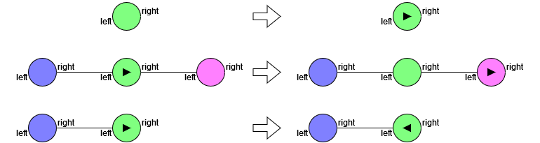
Consider for example the modeling of a particle going left and right on a linear graph by bouncing at the extremities. The linear structure is coded using two ports “left” and “right” on each vertex, while the particle is represented with the presence of a label on some vertex, with two possible values indicating its direction. See Fig. 1 for illustrations of such graphs. The dynamics of the particle is captured by as follows. Suppose that the particle is located at some vertex (in green in Fig. 1), and wants to go to the right. If there is an outgoing edge to the right to an unlabeled vertex (in pink in Fig. 1), the label representing the particle is moved from to (second row of Fig. 1). If there is no outgoing edge to the right (the “right” port of is free), it bounces by becoming a left-going particle (third row of Fig. 1). works symmetrically for a left-going particle.
The behavior of is non-monotonic since the latter situation is a sub-graph of the former, while the particle behaviors in the two cases are clearly incompatible. On Fig. 1, the right hand sides of the second and third rows are comparable by inclusion, but the left hand sides are not. This non-monotonicity involves a missing edge but missing labels may induce non-monotonicity as well. Suppose for the sake of the argument that generates a right-going particle at any unlabeled isolated vertex (first row of Fig. 1). The unlabeled one-vertex graph is clearly a subgraph of any other one where the same vertex is labeled by a right-going particle and has some unlabeled right neighbor. In the former case, the dynamics puts a label on the vertex, while it removes it on the latter case. The new configurations are no longer comparable. See the first and second rows of Fig. 1 for an illustration.
CGD are not necessarily monotonic.
Take , . In a graph , we have isolated vertices and pairwise connected vertices. For the local rule, consider , so the two possible disks (modulo renaming) are the isolated vertex and a pair of connected vertices. There is no graph such that the two disks appear together (otherwise would ask the vertex to be connected and disconnected at the same time). So we can define such that it acts inconsistently on the two disks, since property 4 of local rules does not apply here. But the isolated vertex is included in the connected vertices in the sense of , but the image by , then by are not. ∎
From Corollary 1, we conclude that all non-monotonic CGD are not left Kan extensions as we have developed so far, i.e., based on the subgraph relationship of Def 8. Analyzing the particle CGD in the light of Remark 1 tells us why. Indeed, the subgraph ordering is able to compare a place without any right neighbor with a place with some (left-hand-side of rows 3 and 2 in Fig. 1 for instance). Following Remark 1, in the GT setting, the former situation has less information than the latter: in the former, there is no clue whether the place has a neighbor or not; the dynamics should not be able to specify any behavior for a particle at that place. But clearly, for the corresponding CGD, both situations are totally different: the former is an extremity while the latter is not, and the dynamics specifies two different behaviors accordingly for a particle at that place.
4 Universality of Monotonic Causal Graph Dynamics
We have proven that the set of all CGD is strictly bigger than the set of monotonic ones. However, we prove now that it is not more expressive. By this, we mean that we can simulate any CGD by a monotonic one, i.e., monotonic CGD are universal among general CGD.
More precisely, given a general CGD , a monotonic simulation of consists of encoding, call it , of each graph , and a monotonic CGD such that whenever on the general side, on the monotonic side. Substituting in the latter equation using the former equation, we get , the exact property of the expected simulation: for any , we want some and such that .
4.1 Key Ideas of the Simulation
In this section, we aim at introducing the key elements of the simulation informally and by the mean of the moving particle example.
4.1.1 Encoding the Original Graphs: The Moving Particle Case.
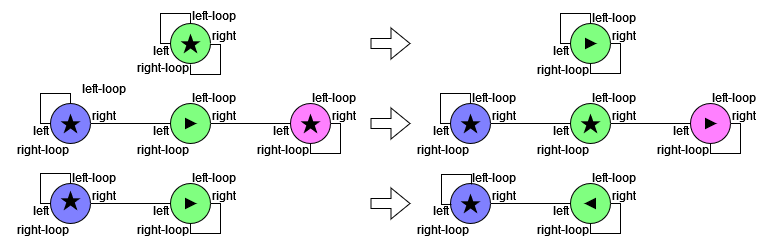
Let us design a monotonic simulation of the particle dynamics. The original dynamics can be made monotonic by replacing the two missing edges at the extremities by easily identifiable loopback edges, making incomparable the two originally comparable situations. For such loopback edges to exist, we need an additional port for each original port, in our case say “left-loop” and “right-loop” for instance. For the case of non-monotonicity with labels, vertices where there is no particle (so originally unlabeled) are marked with a special label, say . Fig. 2 depicts the same evolutions as Fig. 1 after those transformations.
This will be the exact role of the encoding function : the key idea to design a monotonic simulation is to make uncomparable the initially comparable situations. Any missing entity (edge or label) composing an original graph needs to be replaced by a special entity (loopback edge or respectively) in indicating it was originally missing. At the end of the day, for any , we get and no longer comparable.
4.1.2 An Extended Universe of Graphs.
All that remains is to design such that . It is important to note however that the universe of graphs targeted by , which is the domain of , is by design much larger than the original universe. Indeed, each vertex has now a doubled number of ports and the additional label is available. So to be completely done with the task, we need to be able to work not only with graphs generated by the encoding, but also with all the other graphs.
Let us classify the various cases. Firstly, notice that the monotonic counterpart of any graph is “total” in the following sense: all vertices have labels, all original ports have edges, and all edges have labels. However, there also exists partial graphs with free ports and unlabeled vertices in this monotonic universe of graphs. Secondly, uses the additional ports strictly for the encoding of missing edges with loopback edges. But, there are also graphs making arbitrary use of those ports and which are not “coherent” with respect to the encoding. Fig. 3 illustrates the three identified classes: the middle graph is a coherent subgraph of the total graph on the right, and of an incoherent graph on the left. Notice that incoherent edges can always be dropped away to get the largest coherent subgraph of any graph. This is the case on the figure.

4.1.3 Disks in the Extended Universe.
In order to design a local rule of the monotonic CGD , we need to handle disks after encoding. The universe of graphs being bigger than initially, this also holds for disks, and the behavior of will depend on the class of the disk.
Let us first identify the monotonic counterpart of the original disks. They are called “total” disks and correspond to disks of some . For those disks, the injectivity of allows to simply retrieve the corresponding disk of the original graph and invoke the original local rule on it.
An arbitrary disk may not be “total” and exhibit some partiality (free ports, unlabeled vertices or edges). Since is required to be monotonic, it needs to output a subgraph of the original local rule output. More precisely, we need to have for any total disk with . The easiest way to do that is by outputting the empty graph: . (This solution corresponds to the so-called coarse extension proposed for CA in [DBLP:journals/nc/FernandezMS23]; finer extensions are also considered there.)
Last, but not least, an arbitrary disk may make an incoherent use of the additional ports with respect to . In that case, all incoherent information may be ignored by considering the largest coherent subdisk . The behavior of on is then aligned with its behavior on : .
4.1.4 A Larger Radius.
The last parameter of to tune is its radius. It will of course depend on the radius of the local rule of . But it is worth noting that we are actually trying to build more information locally than the original local rule was trying to. Indeed, given a vertex of the original global output, many local rule applications may contribute concurrently to its definition. All of these contributions are consistent with each other of course, but it is possible for some local outputs to indicate some features of that vertex (label, edges) while others do not. If even one of them puts such a label for instance, then there is a label in the global output. It is only if none of them put a label that the global output will not have any label on it. The same holds similarly for ports: a port is free in the global output if it is so on all local outputs. Because the monotonic counterpart needs to specify locally if none of the local rule applications puts such a feature to a vertex, the radius of the monotonic local rule needs to be big enough to include all those local rule input disks. It turns out that the required radius for is , if is the radius of the original local rule , as explained in Fig. 4.
4.2 Formal Definition of the Simulation
Now that we have all the components of the solution, let us make them precise.
4.2.1 The Encoding Function .
The encoding function aims at embedding the graphs of in a universe where ports are doubled and labels are extended with an extra symbol. Set , , and . Ports are considered to be semantically the same as their counterpart while ports are their for loopback edges. For simplicity, let us define the short-hands and for and respectively for the remainder of this section. Since we need to complete partial functions, we introduce the following notation: for any partial function and total function , we define the total function
For simplicity, we write for where runs over . This allows us to define the encoding of any as follows.
The definition of is written to make clear that all original ports are indeed occupied by an edge. The total function is defined based on the partial function as follows.
The definition of deals with original edges for the first case, and with loopback edges for the second, which are the only two possibilities with respect to .
4.2.2 The Disk Encoding Function .
Let us now define the shorthands and for and for any radius . We put the radius as a subscript to make readable the four combinations , , , and . The function aims at encoding original disks as total disks. It is defined as
| (6) |
The reason we apply on the raw result of is that the behavior of (adding loopback edges on each unused port and labels on unlabeled vertices and edges) is not desired at distance for the result to be a disk of radius . More conceptually, is the unique function having the following commutation property, which expresses that is the disk counterpart of . {propositionrep} For any graph , .
Take . After inlining the definition of , we are left to show . For any entity (vertices, labels, edges) at distance at most of , and coincide. At distance , things may differ for the special label and loopback edges, and beyond distance , has no entities at all. However, all these differences are exactly what is removed by . So, we get the expected equality. ∎
4.2.3 Coherent Subgraph Function .
As discussed informally, some graphs in may be ill-formed from the perspective of the encoding by using doubled ports arbitrarily. We define the function that removes the incoherencies.
Since only removes incoherent edges, and since they are stable by inclusion, we trivially have that
Lemma 1.
is monotonic.
4.2.4 The Monotonic Local Rule.
The monotonic local rule is defined in two stages. The first stage is to take a disk in and transform it into something that the original local rule can work with. To do this, we remove any incoherencies with the function , and if the result is total, we restrict it to the correct radius and retrieve its counterpart in the original universe (which is possible because is injective). The original local function can be called on this counterpart. As discussed before, if the coherent sub-disk is not total, we simply output an empty graph. The signature of this function is .
| (7) |
Turning this result in into its counterpart in is more complicated than simply invoking since one have to check that missing entities are really missing, as discussed in Fig. 4. This is the purpose of the second stage leading to the definition of the monotonous local rule which, thanks to its radius , is able to inspect all -disks at distance from .
| (8) |
In this equation, the union of all local results that can contribute to entities attached to is built. In this way, they are all given a chance to say if what was missing in is actually missing. Finally is applied and its result restricted to the sole vertices of and their edges, using the notation of Eq. (1). Those vertices and edges are the only one for which all the possibly contributing disks have been inspected.
is a monotonic local rule.
We first show that is a local rule, that is, to check the four properties of 5.
We need to show that for any isomorphism , there is a conjugate such that . We show that the conjugate of for works. The result is obvious for . In the other case, take :
Consider a family of disks such that . We need to show that . We suppose that for all , (otherwise the result is trivial). First notice that for any family , we have , so . Suppose now some vertex in . So, for each there is some such that which is impossible.
We need a bound such that for all , . We consider the bound given by and show that it works. Indeed the last step of the computation of is precisely a restriction to the vertices of . So .
Consider and . We need and to be consistent. Once again, we suppose that and (otherwise the result is trivial). In order to use the consistency property of , we build . So for any pair of -disks of , and are consistent. In other words, all the original -disks involved in and are consistent with each other. It is particularly true for and . Edges of and are consistent because either they come from and which are consistent, or they are backloop edges added by . Labels are also consistent for the same kind of reason, making and consistent.
We finally show that is monotonic. Take two disks and such that . As is ultimately defined by cases, let us consider first the case where . In this case so we necessarily have . We are left with the case , meaning that is a total disk. Since is monotonic by Lem. 1, . And as a total disk, nothing but incoherences can be added to . So and therefore . So the order is preserved in all cases, and is monotonic. ∎
4.2.5 The Monotonic Simulation.
We finally have the wanted CGD of local rule :
It remains then to show that is indeed a monotonic simulation of , which is achieved with the two next propositions.
Proposition 2.
is monotonic.
Proposition 3.
simulates via the encoding, i.e., .
Proof.
Suppose for some . Since all involved disks in are total and thanks to Prop. 6, the expression of simplifies drastically.
| (9) |
Clearly, does not exhibit any incoherencies and is total, so it is enough to show that to have the equality. This can be done entity by entity. Take a vertex . It comes from some . So it belongs to the inner union of Eq. (9). It is preserved by then by , so it belongs to . Consider now its label . If , there is some with . So the inner union of Eq. (9) labels by . The label is preserved by then by since . So as well. If , this means that none of the put a label on , so is unlabeled in the inner union of Eq. (9). By definition, completes the labeling by at , and preserves this label. So as well. The proof continues similarly for edges and their labels, with an additional care for dealing with loopback edges. ∎∎
5 Conclusion
In this article, we planned to compare CGD and GT frameworks. The very particular route we have chosen for this task led us to identify the class of Monotonic CGD which are both CGD and GT, and happen to be universal among all CGD.
This work was guided by the formal similarities between the two frameworks leading to a list of four questions. The chosen strategy to cope with these questions was to tackle the first one “what is the order?” with the goal of answering positively to the second question “is the union of CGD the supremum of this order?”. This journey led us to identify the subgraph order to structure the set of port graphs instead of considering them independent (more precisely related by the disks only) as the original framework does. This pushes forward the idea of using graph inclusion to express gain of information as proposed by the GT framework, opening a new direction when designing CGD by respecting the order with monotonicity.
One interesting thing to note is that a slight adaptation of the original definition of port graphs allows to represent general CGD as Kan extensions without any encoding. Indeed, the encoding considered in this article leads to a universe of graphs where most of them are ill-formed. By adding explicitly to graphs additional features to represent the positive information that some port is not occupied or some label is missing, it is possible to get a universe where all objects make sense.
An alternative route to answer the four-question list is possible by tackling the first question with the goal of answering the third one (almost) positively, thus falsifying the second one. An order closely related to this route is the “induced subgraph” order stating that is lower than if . This order is stronger than the usual subgraph order but is also very interesting. Fewer graphs are “inducedly consistent” and one may ask if the subclass of CGD definable with this stronger notion of consistency is universal. This might give an idea on whether the result of this article is isolated or, on the contrary, if it follows a common pattern shared with many instances.
Finally, let us not forget the next steps sketched in the introduction, in particular the quotienting of vertex names. In this paper, the notions of isomorphism and renaming-invariance of CGD play no real role. Because GT use a categorical language, this renaming-invariance can be handled by quotienting the objects of the poset, but not the arrows between the objects. This means that there would be now typically many arrows between two objects that the GT framework is able to cope with. Indeed, the formalism of GT was designed to work with objects like abstract graphs where no notion of names or positioning exist, but only their (possible multiple) occurrences in each other. As similar line of thought was already explored for cellular automata in [DBLP:journals/nc/FernandezMS23]. Indeed, cellular automata are typically defined with a global positioning system, but many studies actually only care about the relative positioning of the information. A similar treatment for CGD is for futur work.
References
- [1] Arrighi, P., Dowek, G.: Causal graph dynamics. In: Czumaj, A., Mehlhorn, K., Pitts, A.M., Wattenhofer, R. (eds.) Automata, Languages, and Programming - 39th International Colloquium, ICALP 2012, Warwick, UK, July 9-13, 2012, Proceedings, Part II. Lecture Notes in Computer Science, vol. 7392, pp. 54–66. Springer (2012). https://doi.org/10.1007/978-3-642-31585-5_9, https://doi.org/10.1007/978-3-642-31585-5_9
- [2] Arrighi, P., Martiel, S.: Quantum causal graph dynamics. Physical Review D 96(2), 024026 (2017)
- [3] Arrighi, P., Martiel, S., Perdrix, S.: Reversible causal graph dynamics: invertibility, block representation, vertex-preservation. Nat. Comput. 19(1), 157–178 (2020). https://doi.org/10.1007/S11047-019-09768-0, https://doi.org/10.1007/s11047-019-09768-0
- [4] Fernandez, A., Maignan, L., Spicher, A.: Cellular automata and kan extensions. Nat. Comput. 22(3), 493–507 (2023). https://doi.org/10.1007/S11047-022-09931-0, https://doi.org/10.1007/s11047-022-09931-0
- [5] Maignan, L., Spicher, A.: Global graph transformations. In: Plump, D. (ed.) Proceedings of the 6th International Workshop on Graph Computation Models co-located with the 8th International Conference on Graph Transformation (ICGT 2015) part of the Software Technologies: Applications and Foundations (STAF 2015) federation of conferences, L’Aquila, Italy, July 20, 2015. CEUR Workshop Proceedings, vol. 1403, pp. 34–49. CEUR-WS.org (2015), http://ceur-ws.org/Vol-1403/paper4.pdf