Robust image segmentation model based on binary level set

Abstract

In order to improve the robustness of traditional image segmentation models to noise, this paper models the illumination term in intensity inhomogeneity images. Additionally, to enhance the model’s robustness to noisy images, we incorporate the binary level set model into the proposed model. Compared to the traditional level set, the binary level set eliminates the need for continuous reinitialization. Moreover, by introducing the variational operator GL, our model demonstrates better capability in segmenting noisy images. Finally, we employ the three-step splitting operator method for solving, and the effectiveness of the proposed model is demonstrated on various images.

1 Introduction

With the continuous development of image processing technology, image segmentation plays a key role in various fields such as medical image analysis, 3D reconstruction, and object tracking. In particular, in the context of image segmentation-assisted medical diagnosis, images often suffer from varying degrees of in and noise due to imaging device limitations, which can impact the accuracy of medical diagnosis and treatment. Therefore, for medical images with severe intensity inhomogeneity and noise, a robust and accurate segmentation model is especially important for medical diagnosis. Over the past few decades, numerous segmentation models have been proposed specifically for intensity inhomogeneity and noisy images. Li et al. [6] proposed the Locally Based Fitting (LBF) model, which utilizes the intensity information of local image regions. Zhang [16] modeled intensity inhomogeneity images as Gaussian distributions with different means and variances by exploiting local image region statistics, achieving simultaneous segmentation of intensity inhomogeneity images and the addition of Gaussian noise. Cai et al. [1] introduced the adaptive-scale active contour model based on the maximum a posteriori framework. They constructed an adaptive scale operator and introduced a pixel membership function to achieve segmentation of severely intensity inhomogeneity images. Li et al. [7] introduced the graph space regularization of Markov Random Field to enhance the model’s robustness to noise. For accurate extraction of the region of interest, Ma et al. [10] proposed the Adaptive Local-Fitting-based Active Contour (ALF) method. Yang et al. [11] presented an Adaptive Local Variances-Based Level Set Framework for segmenting intensity inhomogeneity medical images, such as cardiac MR images. Zhang et al. [15] proposed a multi-scale image segmentation model that simultaneously performs image denoising. Ding et al. [2] utilized the Locally Based Fitting (LoG) and optimized Laplacian operator to propose the Laplacian of Gaussian model (LoGLSF). Weng et al. [13] decomposed the observed image into three parts and proposed the Additive Bias Correction (ABC) image segmentation model. Fang et al. [3] proposed an active contour model based on a combination of mixed and locally fuzzy region energies. Wang et al. [12] defined a novel hybrid region intensity fitting energy functional. Jung et al. [5] improved the fidelity term of traditional image segmentation models using L1 norm and proposed the Piecewise Smooth (L1PS) image segmentation model. Wu et al. [14] achieved the non-convex approximation of the Mumford-Shah (MS) model by utilizing a non-convex lp quasi-norm regularization operator and obtained segmentation results using the threshold of K-means clustering. Duan et al. [8] established a new segmented smooth Mumford-Shah model with non-convex Lp regularization term for image labeling and segmentation. Different fitting energy functions have different effects on image segmentation models. Han et al. [4] improved the traditional Euclidean distance and proposed a local data fitting term based on Jeffreys divergence. Liu et al. [9] utilized kernel metric to enhance the model’s robustness to noise. Zhi et al. [17] proposed a hierarchical level set evolution protocol to overcome the edge leakage problem in the level set method (LSM) segmentation process.This paper proposes a segmentation model for intensity inhomogeneity and noisy images. By introducing a binary level set framework and the GL operator, this model eliminates the need for continuous reinitialization and enhances its robustness against noise. The binary level set framework replaces the traditional level set methods, thus avoiding the need for constant reinitialization. Additionally, the inclusion of the GL operator improves the model’s ability to handle noisy images. By employing a three-step segmentation operator approach for solving, the effectiveness of the proposed model is demonstrated on various images.

2 Related work

2.1 LBF model

In order to accurately segment intensity inhomogeneity images, Li et al. proposed the Locally Based Fitting (LBF) model, which utilizes the intensity information of local image regions [6]. The LBF model introduces a variable-scale Gaussian kernel function into the data fitting term, which enables effective segmentation of intensity inhomogeneity images. Therefore, the expression of the LBF model is as follows:

$$\begin{split}\mathcal{M}_{\epsilon}=\mathcal{F}^{LBF}_{\epsilon}+\mu\mathcal{P}(\phi)+\nu\mathcal{L}(\phi).\end{split}$$ (1)

Where $\mu$ and $\nu$ are positive parameters, $\mathcal{P}(\phi)=\frac{1}{2}\int_{\Omega}{(|\nabla\phi(x)-1|^{2})},{\rm d}x$ is the regularization term, $\mathcal{L}(\phi)=\int_{\Omega}{|\nabla H(\phi(x))|},{\rm d}x$ is the length term. The data fitting function is expressed as follows:

$$\begin{split}\mathcal{F}^{LBF}_{\epsilon}(\phi,f_{1},f_{2})=\lambda_{1}\int{[\int{K_{\sigma}(x-y)|I(y)-f_{1}(x)|^{2}T(\phi(y))}\,{\rm d}y]}\,{\rm d}x\\ +\lambda_{2}\int{[\int{K_{\sigma}(x-y)|I(y)-f_{2}(x)|^{2}(1-T(\phi(y)))}\,{\rm d}y]}\,{\rm d}x\end{split}$$ (2)

Where $I:\Omega\subset R^{2}\to R$ represents the image domain, $f_{1}(x)$ and $f_{2}(x)$ denote the approximate intensity values inside and outside the evolving curve $\Gamma$, respectively. $\lambda_{1}$ and $\lambda_{2}$ are positive parameters, $K_{\sigma}$ is a Gaussian kernel function, and $\mathcal{T}(x)$ is the smoothed version of the Heaviside function, defined as:

$$\begin{split}\mathcal{T}_{\epsilon}(x)=\frac{1}{2}[1+\frac{2}{\pi}arctan(\frac{x}{\epsilon})]\end{split}$$ (3)

Although the LBF model has advantages over traditional CV and MS models in segmenting intensity inhomogeneity images, it is sensitive to the initial contour and lacks the ability to segment noisy images.

2.2 Binary Level Set

In order to improve the complex process of continuous reinitialization in traditional level set functions, Lie et al. proposed a binary level set model. Lie et al. suggested using a discontinuous level set function $\phi$ to represent the evolving curve $C$. The definition of $\phi$ is as follows:

$$\phi(x)=\begin{cases}1,&x\in inside(C)\\ -1,&x\in outside(C).\end{cases}$$ (4)

Furthermore, it is assumed that the piecewise constant $\nu$ is represented by the discontinuous binary level set function $\phi$, i.e., $\nu=q_{1}$ when inside$(C)$ and $\nu=q_{2}$ when outside$(C)$.

$$\begin{split}\nu=q_{1}\psi_{1}+q_{2}\psi_{2},\end{split}$$ (5)

Where $\psi_{1}=\frac{1}{2}(1+\phi),\psi_{2}=\frac{1}{2}(1-\phi)$.
Therefore, by combining the binary level set with the Mumford-Shah functional, the following binary level set energy functional is obtained:

$$\begin{split}\mathcal{T}(q_{1},q_{2},\phi)=\frac{1}{2}\int_{\Omega}{(I-\nu)^{2}}\,{\rm d}x+\mu\int_{\Omega}{|\nabla\phi|}\,{\rm d}x\end{split}$$ (6)

Where $\mu\geq 0$, based on the constraint $\phi^{2}=1$, the above energy functional can be transformed into the following unconstrained minimization problem:

$$\begin{split}\min_{q_{1},q_{2},\phi}\mathcal{T}(q_{1},q_{2},\phi),\phi^{2}-1=0\end{split}$$ (7)

Furthermore, by using the Lagrange projection method and augmented Lagrangian method, the aforementioned problem can be transformed into the following expression:

$$\begin{split}\mathcal{H}_{\nu}(q_{1},q_{2},\phi,\lambda)=T(q_{1},q_{2},\phi)+\lambda\int_{\Omega}{(\phi^{2}-1)}\,{\rm d}x+\frac{1}{2}\mu\int_{\Omega}{(\phi^{2}-1)^{2}}\,{\rm d}x.\end{split}$$ (8)

Where $\lambda>0$ and $\mu>0$ are the Lagrange multipliers and penalty parameters.

3 The proposed model

To correct the intensity inhomogeneity of the image and enhance the model’s robustness to noise, we introduce the bias field correction $I=bc$ model into the binary level set assumption. Furthermore, the following model assumptions are proposed.

$$\begin{split}E(c_{1},c_{2},\phi)=\lambda_{1}\int_{\Omega}{(I-bc_{1})^{2}(1+\phi)^{2}}dx+\lambda_{2}\int_{\Omega}{(I-bc_{2})^{2}(1-\phi)^{2}}dx\\ +\mu\int_{\Omega}{|\nabla\phi|^{2}}dx\end{split}$$ (9)

Where $\lambda_{1}$, $\lambda_{2}$, $\mu$, and $\nu$ are non-negative constants. The regularization term $\int_{\Omega}|\nabla\phi|^{2}dx$ effectively suppresses the oscillation of the level set during the evolution process and enhances the model’s robustness to noise. To further solve the above functional, we transform it into the following unconstrained minimization problem.

$$\begin{split}min_{c_{1},c_{2},\phi}E(c_{1},c_{2},\phi)=\lambda_{1}\int_{\Omega}{(I-bc_{1})^{2}(1+\phi)^{2}}dx+\lambda_{2}\int_{\Omega}{(I-bc_{2})^{2}(1-\phi)^{2}}dx\\ +\mu\int_{\Omega}{|\nabla\phi|^{2}}dx+\nu\int_{\Omega}{(\phi^{2}-1)^{2}}dx\end{split}$$ (10)

Usually, a larger parameter $\nu$ is chosen to make the variable $\phi^{2}$ closer to 1. The last term, $\int_{\Omega}(\phi^{2}-1)^{2}dx$, is included to ensure that the level set remains within the binary range.

4 Algorithm implementation

To solve the problem in Eq.(10), we update the variables $c_{1}$, $c_{2}$, $b$, and the variable $\phi$ using iterative minimization algorithms and a three-step splitting operator. Therefore, we divide it into the following two parts for solving: (1) To solve the subproblem of $c_{1}$ and $c_{2}$, we fix the variables $\phi$ and $b$ and solve for

$$\begin{split}min_{c_{1},c_{2}}E(c_{1},c_{2})=\lambda_{1}\int_{\Omega}{(I-bc_{1})^{2}(1+\phi)^{2}}dx+\lambda_{2}\int_{\Omega}{(I-bc_{2})^{2}(1-\phi)^{2}}dx\end{split}$$ (11)

where the last two terms in Eq.(10) are omitted since they are independent of the variables $c_{1}$ and $c_{2}$.

$$\begin{split}min_{c_{1},c_{2}}E(c_{1},c_{2})=\lambda_{1}\int_{\Omega}{(I-bc_{1})^{2}(1+\phi)^{2}}dx+\lambda_{2}\int_{\Omega}{(I-bc_{2})^{2}(1-\phi)^{2}}dx\end{split}$$ (12)

The last two terms in (10) are omitted because they are independent of the variables $c_{1}$ and $c_{2}$. (2) To solve the subproblem of $b$, we fix the variables $\phi$, $c_{1}$, and $c_{2}$, and solve for

$$\begin{split}min_{b}E(b)=\lambda_{1}\int_{\Omega}{(I-bc_{1})^{2}(1+\phi)^{2}}dx+\lambda_{2}\int_{\Omega}{(I-bc_{2})^{2}(1-\phi)^{2}}dx\end{split}$$ (13)

$$\begin{split}min_{\phi}E(\phi)=\lambda_{1}\int_{\Omega}{(I-bc_{1})^{2}(1+\phi)^{2}}dx+\lambda_{2}\int_{\Omega}{(I-bc_{2})^{2}(1-\phi)^{2}}dx\\ +\mu\int_{\Omega}|\nabla\phi|^{2}dx+\nu\int_{\Omega}{(\phi^{2}-1)^{2}}dx\end{split}$$ (14)

(3)Solve the $\phi$ sub-problem by fixing the variables $c_{1},c_{2},b$ and finding the solution.

$$\begin{split}min_{\phi}E(\phi)=\lambda_{1}\int_{\Omega}{(I-bc_{1})^{2}(1+\phi)^{2}}dx+\lambda_{2}\int_{\Omega}{(I-bc_{2})^{2}(1-\phi)^{2}}dx\\ +\mu\int_{\Omega}|\nabla\phi|^{2}dx+\nu\int_{\Omega}{(\phi^{2}-1)^{2}}dx\end{split}$$ (15)

By using the gradient descent method, we can obtain the values of $c_{1}$ and $c_{2}$ as follows:

$$\begin{split}c_{1}=\frac{\int_{\Omega}{Ib(1+\phi)^{2}}dx}{\int_{\Omega}{b^{2}(1+\phi)^{2}}dx}\end{split}$$ (16)

$$\begin{split}c_{2}=\frac{\int_{\Omega}{Ib(1-\phi)^{2}}dx}{\int_{\Omega}{b^{2}(1-\phi)^{2}}dx}\end{split}$$ (17)

By fixing the variables $c_{1}$, $c_{2}$, and $\phi$, we iteratively update the variable $b$ and obtain the following equation:

$$\begin{split}b=\frac{\int_{\Omega}{\lambda_{1}I(1+\phi)^{2}c_{1}+\lambda_{2}I(1-\phi)^{2}c_{2}dx}}{\int_{\Omega}{\lambda_{1}c_{1}^{2}(1+\phi)^{2}+\lambda_{2}c^{2}_{1}(1-\phi)^{2}dx}}\end{split}$$ (18)

Next, we will update the iterative variable $\phi$ using the three-step splitting operator. Therefore, we first apply the gradient descent method to Eq.(15) and obtain:

$$\begin{split}\frac{\partial\phi}{\partial t}=-\lambda_{1}(I-bc_{1})^{2}(1+\phi)+\lambda_{2}(I-bc_{2})^{2}(1-\phi)+\mu\nabla\phi-2\nu\phi(\phi^{2}-1)\end{split}$$ (19)

To simplify the solving process, we let

$$\begin{split}A=\lambda_{1}(I-bc_{1})^{2},B=\lambda_{2}(I-bc_{2})^{2}\end{split}$$ (20)

Next, we will use the three-step splitting operator method to solve the above process: 第一步： First step: Let $\phi^{n}(x)$ be the level set function computed in the nth loop. We solve the initial value problem originating from the data term:

$$\begin{split}\begin{cases}\frac{\partial\phi}{\partial t}=-A(1+\phi)+B(1-\phi)\\ \phi(x,t)|_{t=0}=\phi^{n}(x)\end{cases}\end{split}$$ (21)

The iteration continues until we obtain the final result $\phi^{n+1,1}(x)=\phi(x,T_{1})$, where $T_{1}>0$. Second step: Solving the nonlinear diffusion equation generated by the regularization term.

$$\begin{split}\frac{\partial\phi}{\partial t}=\mu\nabla\phi\end{split}$$ (22)

With the initial value $\phi(x,t)|_{t}=\phi^{n+1,1}(x)$, we obtain the solution at the second time step as $\phi^{n+1,2}(x)=\phi(x,T_{2})$, where $T_{2}>0$. The third step: Based on the initial value $\phi(x,t)|_{t}=0=\phi^{n+1,2}(x)$, we obtain the following nonlinear equation:

$$\begin{split}\frac{\partial\phi}{\partial t}=-2\nu\phi(\phi^{2}-1)\end{split}$$ (23)

Until a certain time $T_{3}>0$, we obtain the solution at the third time step as $\phi^{n+1}(x)=\phi(x,T_{3})$. To solve the first step, to avoid the restriction of time step, we adopt the implicit scheme as follows:

$$\begin{split}\frac{\phi^{n+1,1}-\phi^{n}}{\tau_{1}}=-A(1+\phi^{n+1,1})+B()-\phi^{n+1,1}\end{split}$$ (24)

$\tau_{1}>0$ is the time step. Therefore, we obtain the result of the first step as:

$$\begin{split}\phi^{n+1,1}=\frac{\phi^{n}-\tau_{1}(A-B)}{1+\tau_{1}(A+B)}\end{split}$$ (25)

In the second step, we further discretize the time as follows:

$$\begin{split}\frac{\phi^{n+1,2}-\phi^{n+1,1}}{\tau_{2}}=\mu\nabla\phi^{n+1,2}\end{split}$$ (26)

Where $\tau_{2}>0$ is the time step. By utilizing the Fast Fourier Transform, we obtain the solution to the discretized equation mentioned above:

$$\begin{split}\phi^{n+1,2}=\mathscr{F}^{-1}(\frac{\mathscr{F}(\phi^{n+1,1})}{1-\mu\tau_{2}\mathscr{F}(\Delta)}).\end{split}$$ (27)

Where $\mathscr{F}$ denotes the Fourier transform, and $\mathscr{F}^{-1}$ denotes the inverse Fourier transform. In the third step, utilizing the projection method, we obtain the following solution:

$$\phi^{k+1}=\begin{cases}1&\phi^{n+1,2}\geq 0\\ -1&\phi^{n+1,2}<0.\end{cases}$$ (28)

4.1 Experiments

This paper adopts the $JS$ and $Dice$ coefficients as evaluation metrics for image segmentation results. The parameter settings are $\lambda_{1}=\lambda_{2}$, $\tau_{1}=$. $TP$ represents true positives, which are positive samples correctly predicted by the model. $TN$ represents true negatives, which are negative samples correctly predicted by the model. $FP$ represents false positives, which are negative samples incorrectly predicted as positive by the model. $FN$ represents false negatives, which are positive samples incorrectly predicted as negative by the model. The specific definitions of $JS$ and $Dice$ coefficients are as follows:

$$\begin{split}Dice=\frac{2*TP}{TP+FP+TP+FN}\end{split}$$ (29)

$$\begin{split}JS=\frac{TP}{TP+FP}\end{split}$$ (30)

With the development of computer-aided medical imaging technology, medical image segmentation has been widely used in medical research, clinical diagnosis, lesion analysis, and other areas. The purpose of medical segmentation is to extract lesions or identify abnormalities from MRI and CT images, providing a basis for further clinical studies. However, due to the diversity of medical images and the influences of factors such as noise, tissue motion, and bias fields during the imaging process, medical image segmentation remains a challenging task. To further validate the performance and efficiency of the proposed model in segmenting medical images, we conducted qualitative and quantitative analyses on four MRI images. The segmentation results are shown in Fig. 1. From a visual perspective, in the brain tumor images in the first and fourth rows, although the LSACM, LBF, and DRLSE-ADMM models can locate the boundaries of the targets, they tend to oversegment due to the influence of brighter areas such as the skull. Moreover, due to the blurred nature of tumor edge regions, the ABC model exhibits undersegmentation in the fourth row. Specifically, in the brain CT image shown in the second row, only LBF and LSACM achieve complete segmentation of the target region, but fail to segment some gray matter sulci. In comparison, the proposed model demonstrates higher accuracy in segmenting medical images than other models. Fig. 3 presents line graphs illustrating the quantitative metrics for the aforementioned four images. It can be observed that the proposed model achieves the highest Jaccard similarity (JS) value, which remains stable, thus validating its effectiveness in segmenting MRI images.

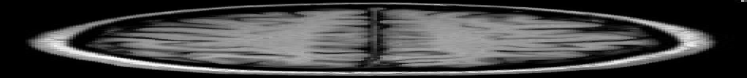
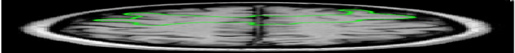
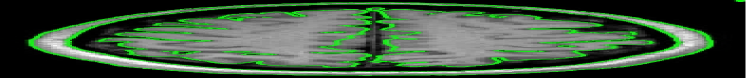
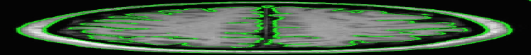
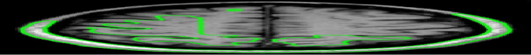
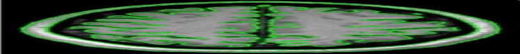
Figure 1: (a)The original image(b)ABC(c)LSACM(d)LBF(e)DRLSE-ADMM(f)OURS

Regardless of whether it is low-light images, medical images, or real-world images, they often contain varying degrees of noise and intensity inhomogeneity. This requires the proposed algorithm to possess a certain robustness to images with noise and intensity inhomogeneity. To validate the segmentation performance of the proposed model on severely noisy images, the following experiment was designed. Figure LABEL:img8 displays columns of the original images with initial contours, the segmentation results of the original images, and the segmentation results after adding the same type of noise. Rows display three different images and the segmentation results after adding various types and degrees of noise. The first and second images have been respectively added with salt-and-pepper noise with a variance of 0.8, Gaussian white noise with variances of 0.4 and 0.6, and speckle noise with variances of 0.4 and 0.8. The third image has been added with salt-and-pepper noise with a variance of 0.5, Gaussian white noise with a variance of 0.3, and speckle noise with a variance of 0.3. It is well-known that image quality decreases to varying degrees when severe noise is added. However, from the experimental results, it can be observed that the segmentation accuracy did not change significantly. Particularly, the third image demonstrates that even when both intensity inhomogeneity and noise are present, the proposed model still achieves good segmentation results.

Figure 2: Our model was applied to segment noisy images, and the segmentation results are as shown above. From left to right, they correspond to: original images with initial contours, segmentation results of the original images, images with added Speckle noise, images with added Salt and pepper noise, and images with added Gaussian noise.

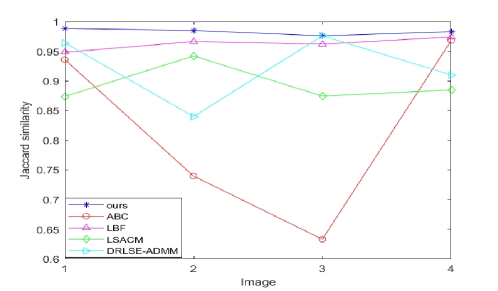
Figure 3: The line graph corresponding to the segmentation results in Figure 1.

5 Conclusion

This paper proposes an image segmentation and bias field correction model based on binary level sets. Additionally, due to the introduction of the GL operator, the proposed model in this paper exhibits good robustness to noise and has been compared with other relevant models to demonstrate its effectiveness. Furthermore, we will further improve the proposed model’s ability to handle high-noise images and optimize the modeling framework.

References

- Cai et al. [2018] Q. Cai, H. Liu, S. Zhou, J. Sun, J. Li, An adaptive-scale active contour model for inhomogeneous image segmentation and bias field estimation, Pattern Recognition 82 (2018) 79–93.
- Ding et al. [2017] K. Ding, L. Xiao, G. Weng, Active contours driven by region-scalable fitting and optimized laplacian of gaussian energy for image segmentation, Signal Processing 134 (2017) 224–233.
- Fang et al. [2021] J. Fang, H. Liu, L. Zhang, J. Liu, H. Liu, Region-edge-based active contours driven by hybrid and local fuzzy region-based energy for image segmentation, Information Sciences 546 (2021) 397–419.
- Han and Wu [2020] B. Han, Y. Wu, Active contour model for inhomogenous image segmentation based on jeffreys divergence, Pattern Recognition 107 (2020) 107520.
- Jung [2017] M. Jung, Piecewise-smooth image segmentation models with l1 data-fidelity terms, J. Sci. Comput. 70 (2017) 1229–1261.
- Li et al. [2008] C. Li, C.Y. Kao, J.C. Gore, Z. Ding, Minimization of region-scalable fitting energy for image segmentation, IEEE Transactions on Image Processing 17 (2008) 1940–1949.
- Li et al. [2020a] Y. Li, G. Cao, T. Wang, Q. Cui, B. Wang, A novel local region-based active contour model for image segmentation using bayes theorem, Information Sciences 506 (2020a) 443–456.
- Li et al. [2020b] Y. Li, C. Wu, Y. Duan, The tvp regularized mumford-shah model for image labeling and segmentation, IEEE Transactions on Image Processing 29 (2020b) 7061–7075.
- Liu et al. [2018] Y. Liu, C. He, Y. Wu, Variational model with kernel metric-based data term for noisy image segmentation, Digital Signal Processing 78 (2018) 42–55.
- Ma et al. [2019] D. Ma, Q. Liao, Z. Chen, R. Liao, H. Ma, Adaptive local-fitting-based active contour model for medical image segmentation, Signal Processing: Image Communication 76 (2019) 201–213.
- Shu et al. [2023] X. Shu, Y. Yang, J. Liu, X. Chang, B. Wu, Alvls: Adaptive local variances-based levelset framework for medical images segmentation, Pattern Recognition 136 (2023) 109257.
- Wang et al. [2018] L. Wang, J. Zhu, M. Sheng, A. Cribb, S. Zhu, J. Pu, Simultaneous segmentation and bias field estimation using local fitted images, Pattern Recognition 74 (2018) 145–155.
- Weng et al. [2021] G. Weng, B. Dong, Y. Lei, A level set method based on additive bias correction for image segmentation, Expert Systems with Applications 185 (2021) 115633.
- Wu et al. [2021] T. Wu, J. Shao, X. Gu, M.K. Ng, T. Zeng, Two-stage image segmentation based on nonconvex ℓ2−ℓp approximation and thresholding, Applied Mathematics and Computation 403 (2021) 126168.
- Zhang et al. [2019] H. Zhang, L. Tang, C. He, A variational level set model for multiscale image segmentation, Information Sciences 493 (2019) 152–175.
- Zhang et al. [2016] K. Zhang, L. Zhang, K.M. Lam, D. Zhang, A level set approach to image segmentation with intensity inhomogeneity, IEEE Transactions on Cybernetics 46 (2016) 546–557.
- Zhi and Shen [2018] X.H. Zhi, H.B. Shen, Saliency driven region-edge-based top down level set evolution reveals the asynchronous focus in image segmentation, Pattern Recognition 80 (2018) 241–255.