Enhancing Security in Multi-Robot Systems through Co-Observation Planning, Reachability Analysis, and Network Flow

Abstract

This paper addresses security challenges in multi-robot systems (MRS) where adversaries may compromise robot control, risking unauthorized access to forbidden areas. We propose a novel multi-robot optimal planning algorithm that integrates mutual observations and introduces reachability constraints for enhanced security. This ensures that, even with adversarial movements, compromised robots cannot breach forbidden regions without missing scheduled co-observations. The reachability constraint uses ellipsoidal over-approximation for efficient intersection checking and gradient computation. To enhance system resilience and tackle feasibility challenges, we also introduce sub-teams. These cohesive units replace individual robot assignments along each route, enabling redundant robots to deviate for co-observations across different trajectories, securing multiple sub-teams without requiring modifications. We formulate the cross-trajectory co-observation plan by solving a network flow coverage problem on the checkpoint graph generated from the original unsecured MRS trajectories, providing the same security guarantees against plan-deviation attacks. We demonstrate the effectiveness and robustness of our proposed algorithm, which significantly strengthens the security of multi-robot systems in the face of adversarial threats.

I Introduction

Multi-robot systems (MRS) have found wide applications in various fields. While offering numerous advantages, the distributed nature and dependence on network communication render the MRS vulnerable to cyber threats, such as unauthorized access, malicious attacks, and data manipulation [1]. This paper addresses a specific scenario in which robots are compromised by attacker and directed to forbidden regions, which may contain security-sensitive equipment or human workers. Such countering deliberate deviations, termed plan-deviation attacks, are identified and addressed in previous studies [2, 3, 4, 5, 6]. As a security measure, we utilized onboard sensing capabilities of the robots to perform inter-robot co-observations and check for unusual behavior. These mutual observation establish a co-observation schedule alongside the path, ensuring that any attempts by a compromised robot to violate safety constraints (such as transgressing forbidden regions) would break the observation plan and be promptly detected.

A preliminary version of the paper was presented in [6, 5]. Extanding the grid-world solution from [2] to continuous configuration spaces, we incorporate the co-observation planning as constraints in the ADMM-based trajectory optimization solver to accomodate for more flexible objectives. In this paper, we incorporate additional reachability analysis during the planning phase, incorporating constraints based on sets of locations that agents could potentially reach, referred to as reachability regions, as a novel perspective to the existing literature. This approach enforces an empty intersection between forbidden regions and the reachability region during trajectory optimization, preventing undetected attacks if an adversary gains control of the robots. Inspired by the heuristic sampling domain introduced by [7] within the context of the $\mathtt{RRT^{*}}$ path planning algorithm, we utilize an ellipsoidal boundary to constrain the search space and formulate the ellipsoid as the reachability region constraint. We present a mathematical formulation of reachability regions compatible with the solver in [6] as a spatio-temporal constraint.

However, such plans are not guaranteed to exist, and the secured trajectory always come at the cost of overall system performance. As an extension of the previous works [6, 5], we also address the feasibility and optimality challenges. For a MRS with unsecured optimal trajectorys (without security constraints), we introduce redundant robots and formed into sub-teams with the original ones. These redundant robots are assigned the task of establishing additional co-observations, termed cross-trajectory co-observations, within and across different sub-teams. The proposed algorithm focuses on the movement plans for the additional robots, distinct from those dedicated to task objectives, indicating when they should stay with their current sub-team and when they should deviate to join another. This strategy allows sub-teams to preserve the optimal unsecured trajectories (as illustrated in Figure 1) without requiring the entire sub-team to maintain close proximity to other teams during co-observation events. The cross-trajectory co-observation problem is transformed as a multi-agent path finding problem on roadmap (represented as directed graph) and solved as a network flow problem [8].

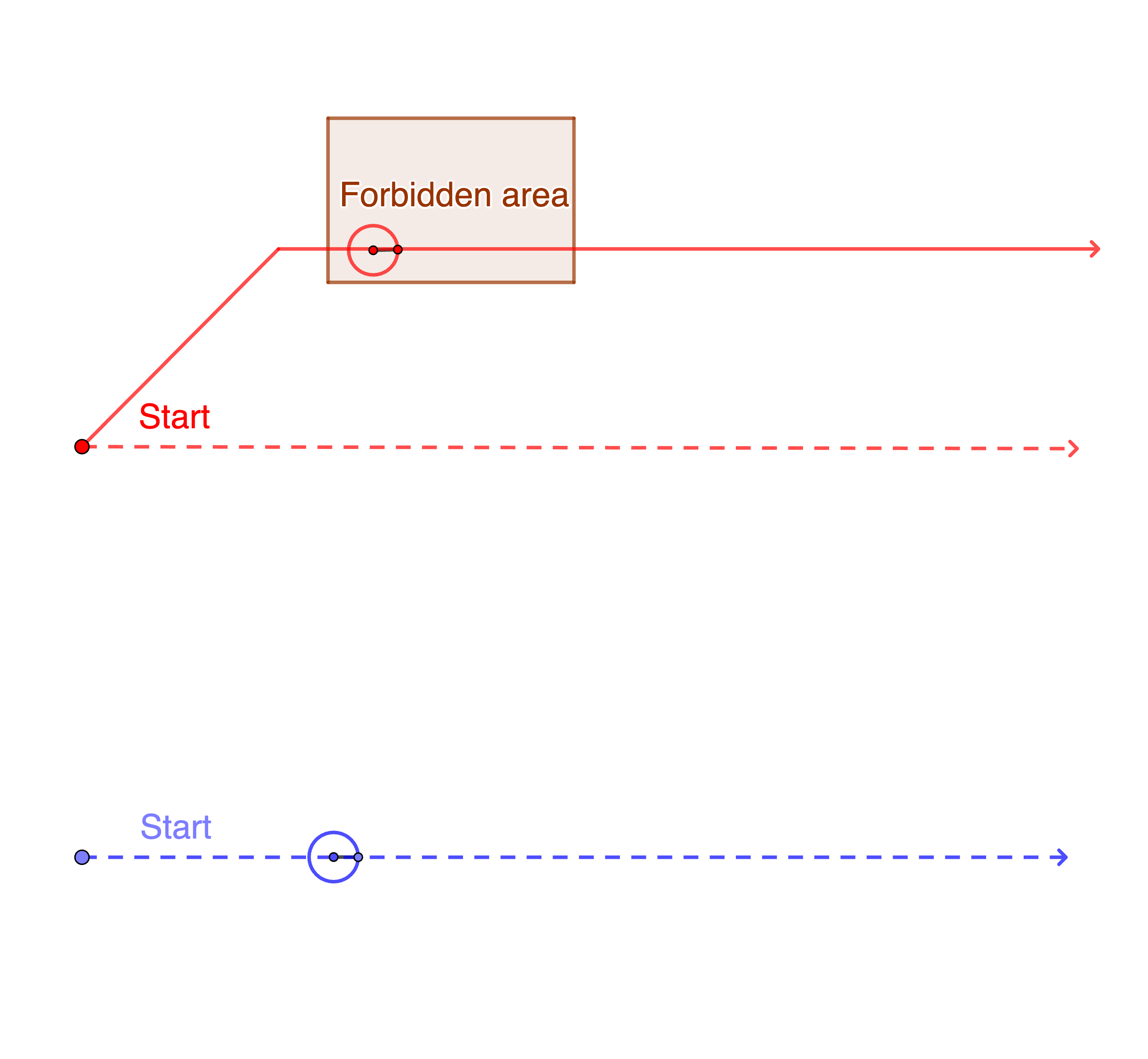
(a) Plan-deviation attack

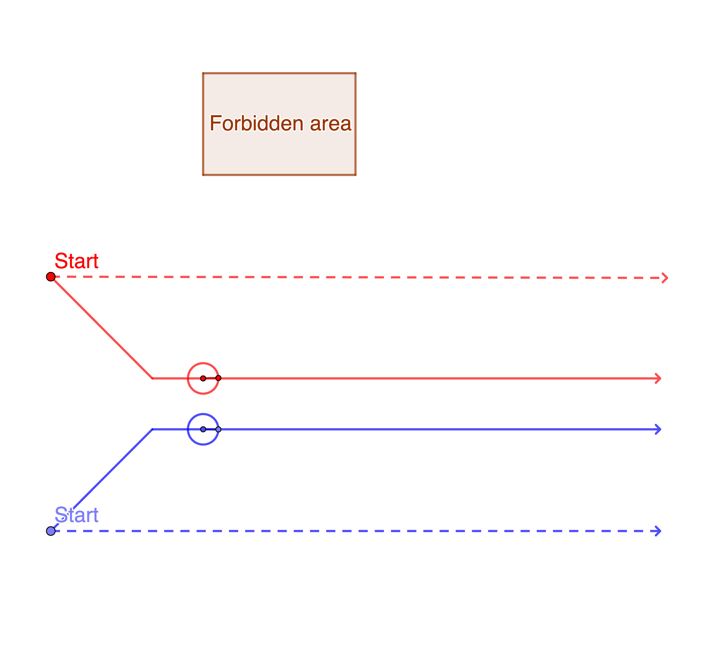
(b) Co-observation

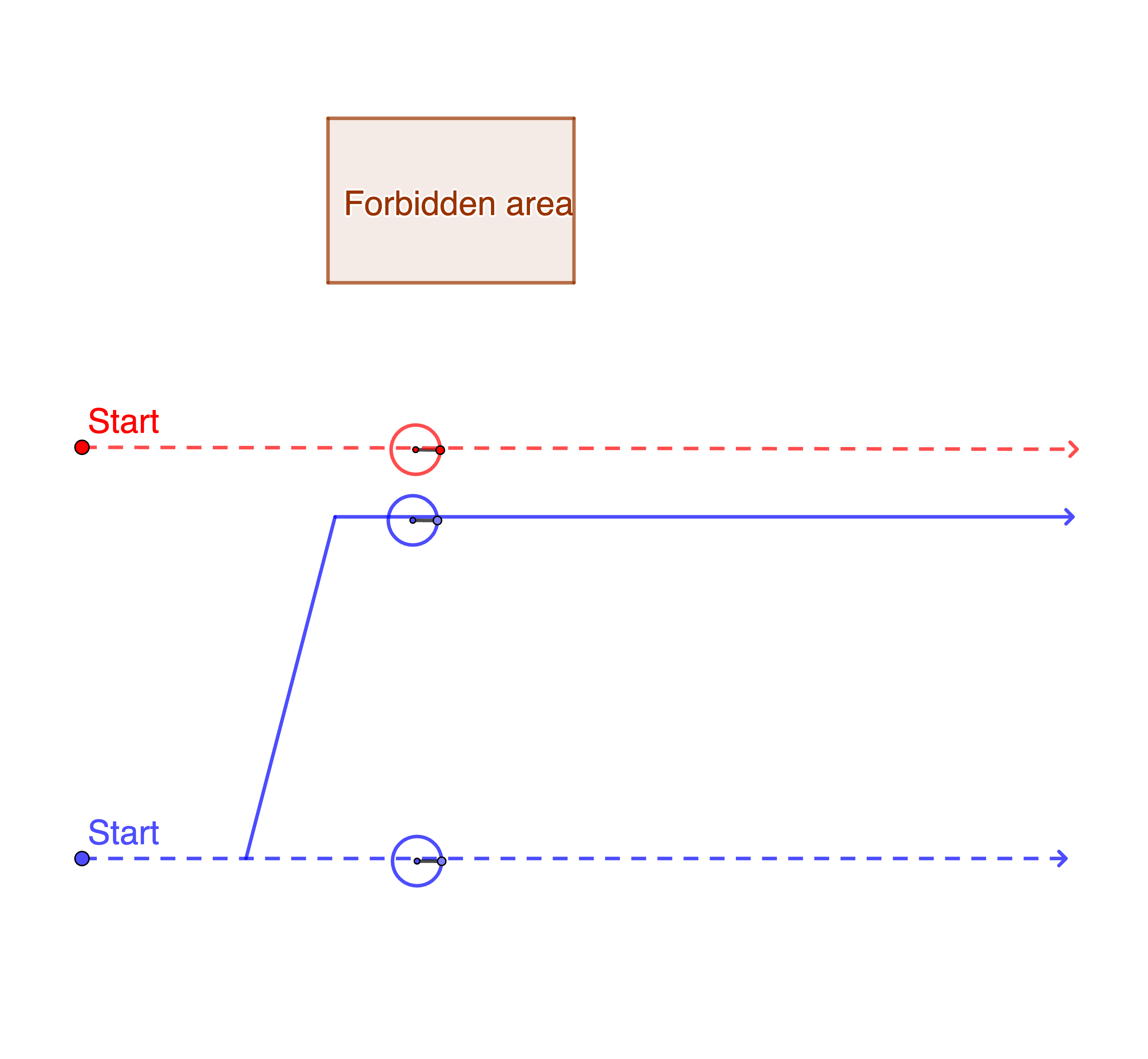
(c) Cross-trajectory co-observation

Figure 1: 1b Limited by the co-observation requirement, both red and blue robot follow the co-observation secured routes (solid lines) and abandon the optimal ones (dashed line). 1c Through cross-trajectory co-observations, the blue team sends one robot to follow the red team (solid blue line) and performs co-observation while having the rest of the robots following the optimal trajectory.

Related research. Trajectory planning problem of MRS systems remained as a subject of intense study for many decades, and optimization is a common approaches in such area. Optimization based approaches are customizable to a variable of constraints (e.g. speed limit, avoid obstacles) and task specifications (e.g. maximum surveillance coverage, minimal energy cost). In constract to our work in Section II, many motion planning tasks require a non-convex constraint problem formulation, most contributors focused on convex problems, and only allow for a few types of pre-specified non-convex constraints through convexification[9][10][11]. Several optimization techniques like MIQP [12] and ADMM [13] have been used to reduce computational complexity, and to incorporate more complex non-convex constraints.

Graph-based search is another extensively explored approach in trajectory planning problems, such as formation control [14, 15] and Multi-Agent Path Finding (MAPF) problems [16]. In traditional MAPF formulations, environments are abstracted as graphs, with nodes representing positions and edges denoting possible transitions between positions and solved as a network flow problem [8, 17]. This formulation allows for the application of combinatorial network flow algorithms and linear program techniques, offering efficient and more flexible solutions to the planning problem.

In Section II, we incorporate reachability constraints to increase overall security Reachability analysis is a important step in the security and safety verification synthesis for cyber-physical systems (CPSs) [18, 19]. One typical approach involves computing an over-approximation of the reachable space for checking safety properities. Previous studies [20, 21, 22] often use geometric representation, such as zonotopes and ellipsoids, as a compact enclosure of the reachability sets. In the realm of online safety assessment against cyber attacks, [23] computed the reachable set of CPS states achievable by potential cyber attacks and compared it with the safe region, set based on current state estimation and environmental conditions.

Paper contributions. In this paper, two main contributions have been presented.

• We present an innovative method to integrate reachability analysis into the ADMM-based optimal trajectory solver for multi-robot systems, preventing attackers from executing undetected attacks by simultaneously entering forbidden areas and adhering to co-observation schedules.

• We introduce additional robots to form sub-teams for both intra-sub-team and cross-sub-team co-observations. A new co-observation planning algorithm is formulated that can generate a resilient multi-robot trajectory with a co-observation plan that still preserve the optimal performance against arbitrary tasks. We also find the minimum redundant robots required for the security.

Paper Outline. The rest of this paper is organized as follows. Section IIprovide an overview of the ADMM-based optimal trajectory solver and introduce the security constraints including co-observation constraints and ellipsoidal reachability constraints. Section III introduced the enhanced security planning algorithm by the incorporation of redundant robots for cross-trajectory co-observation. Section IV concludes this article.

II Secured Multi-robot trajectory planning

We formulate the planning problem as an optimal trajectory optimization problem to minimize arbitrary smooth objective functions. We denote as $q_{ij}\in m$ the position of agent $i$ at the discrete-time index $j$, with $m$ representing the dimension of the state space. For a total of $n_{p}$ robots, and a task time horizon of $T$, a total of $n_{p}$ trajectories can be represented as an aggregated vector $\mathbf{q}\in nmT$. The overall goal is to minimize or maximize an objective function $\varPhi(\mathbf{q})$ under a set of nonlinear constraints described by a set $\Omega$, which is given by the intersection of spatio-temporal sets given by traditional path planning constraintsand the security constraints (co-observation schedule, reachability analysis). Formally:

$$\begin{split}\min/\max&\quad\varPhi(\mathbf{q})\\ \textrm{subject to}&\quad\mathbf{q}\in\Omega.\end{split}$$ (1)

To give a concrete example of the cost $\varPhi$ and the set $\Omega$, we introduce a representative application that will be used for all the simulations throughout the paper.

Example 1

Robots are tasked to navigate, collecting sensory data to construct a corresponding map for the slowly-varying field, denoted as $\mathbf{x}$, of an unknown environment (see Figure 3b). The map comprises points of interest arranged on a grid, each associated with a slowly-changing value. Our goal is to find paths that minimize uncertainty and effectively reconstruct the field. We associate a Kalman Filter (KF) (cf. [24]) to each point $j$, and use it to track the uncertainty through its estimated covariance $P_{j}$. The updates of the filters are based on measurements from the robot centered at $q$, and we use a Gaussian radial basis function modeling spatially-varying measurement quality. The optimization objective $\varPhi(\mathbf{q})$ is written as the maximum uncertainty $\max_{j}P_{j}$ (detailed formulation can be found in [6]).

To incorporate the security against malicious deviations (through co-observation and reachability analysis) as constraints in the optimal trajectory planning problem, we define the security as:

Definition 1

A multi-robot trajectory plan is secure again plan-deviation attacks if it ensure that any potential deviations to these forbidden regions will cause the corresponding robot to miss their next co-observation with other robots.

II-A Preliminaries

II-A1 Differentials

We define the differential of a map $f(x):m\to n$ at a point $x_{0}$ as the unique matrix $\partial_{x}f\in n\times m$ such that

$$\left.\frac{\mathrm{d}}{\mathrm{d}t}f\bigl{(}x(t)\bigr{)}\right|_{t=0}=\partial_{x}f\bigl{(}x(0)\bigr{)}\dot{x}(0)$$ (2)

where $t\mapsto x(t)\in n$ is a smooth parametric curve such that $x(0)=x$ with any arbitrary tangent $\dot{x}(0)$. For brevity we will use $\dot{f}$ for $\frac{\mathrm{d}}{\mathrm{d}t}f$ and $\partial_{x}f$ for $\frac{\partial f}{\partial x}$.

With a slight abuse of notation, we use the same notation $\partial_{x}f$ for the differential of a matrix-valued function with scalar arguments $f:R\to m\times n$. Note that in this case (2) is still formally correct, although the RHS needs to be interpreted as applying $\partial_{x}f$ as a linear operator to $\dot{x}$.

II-A2 Householder rotations

We define a differentiable transformation to a canonical ellipse that is used in the derivation of the reachability constraints in Sections II-C and II-H. This transformation includes a rotation derived from a modified version of Householder transformations [25]. With respect to the standard definition, our modification ensures that the final operator is a proper rotation (i.e., not a reflection). We call our version of the operator a Householder rotation. In this section we derive Householder rotations and their differentials for the 3-D case; the 2-D case can be easily obtained by embedding it in the $z=0$ plane.

Definition 2

Let $\nu_{\mathcal{F}}$ and $\nu_{\mathcal{E}}$ be two unitary vectors ($\lVert\nu_{\mathcal{F}}\rVert=\lVert\nu_{\mathcal{E}}\rVert=1$). Define the normalized vector $u$ as

$$u^{\prime}=\nu_{\mathcal{F}}+\nu_{\mathcal{E}},\quad u=\frac{u^{\prime}}{\lVert u^{\prime}\rVert}.$$ (3)

The Householder rotation $H(\nu_{\mathcal{F}},\nu_{\mathcal{E}})$ is defined as

$$H(\nu_{\mathcal{F}},\nu_{\mathcal{E}})=2uu^{\mathrm{T}}-I.$$ (4)

Here $H$ is a rotation mapping $\hat{\nu_{\mathcal{F}}}$ to $\hat{\nu_{\mathcal{E}}}$, as shown by the following.

Proposition 1

The matrix $H$ has the following properties:

1. It is a rotation, i.e.

   1. $H^{\mathrm{T}}H=I$;

   2. $\det(H)=1$.

2. $\nu_{\mathcal{E}}=H\nu_{\mathcal{F}}$.

Proof:

See Appendix -A. ∎

We compute the differential of $H$ implicitly using its definition (2). We use the notation $[v]_{\times}\!:3\to 3\times 3$ to denote the matrix representation of the cross product with the vector $v$, i.e.,

$$\begin{bmatrix}v_{1}\\ v_{2}\\ v_{3}\end{bmatrix}_{\times}=\begin{bmatrix}0&-v_{3}&v_{2}\\ v_{3}&0&-v_{1}\\ -v_{2}&v_{1}&0\end{bmatrix},$$ (5)

such that $[v]_{\times}w=v\times w$ for any $w\in 3$.

Proposition 2

Let $\nu_{\mathcal{F}}(t)$ represent a parametric curve. Then

$$\dot{H}=H[-2M\dot{\nu}_{\mathcal{F}}]_{\times}\!,$$ (6)

where the matrix $M\in 3\times 3$ is given by

$$M=[u]_{\times}\frac{\left(I-uu^{\mathrm{T}}\right)\left(I-\nu_{\mathcal{F}}\nu_{\mathcal{F}}^{\mathrm{T}}\right)}{\lVert u^{\prime}\rVert\lVert\nu_{\mathcal{F}}\rVert}.$$ (7)

Proof:

See Appendix -B. ∎

II-A3 Alternating Directions Method of Multipliers (ADMM)

The basic idea of the ADMM-based solver introduced in [6] is to separate the constraints from the objective function using a different set of variables $\mathbf{z}$, and then solve separately in (1). More specifically, we rewrite the constraint $\mathbf{q}\in\varOmega$ using an indicator function $\varTheta$, and include it in the objective function (details can be found in [6]). We allow $\mathbf{z}=D(\mathbf{q})$ to replicate an arbitrary function of the main variables $\mathbf{q}$ (instead of being an exact copy in general ADMM formulation), to transform constraint $\mathbf{q}\in\Omega$ to $D(\mathbf{q})\in\mathcal{Z}$ to allow for an easier projection step in Equation 9b. In summary, we transform Equation 1 into

$$\max\quad\varPhi(\mathbf{q})+\varTheta(\mathbf{z})$$ (8)

$$\begin{array}[]{r@{\quad}c}s.t.&D(\mathbf{q})-\mathbf{z}=0\end{array}$$

where $D(\mathbf{q})=[D_{1}(\mathbf{q})^{T},\dots,D_{l}(\mathbf{q})^{T}]^{T}$ is a vertical concatenation of different functions for different constraints. This makes each constraint set $\mathcal{Z}_{i}$ independent and thus can be computed separately in later updating steps. $D_{i}(\mathbf{q})$ is chosen that the new constraint set $\mathcal{Z}_{i}$ becomes simple to compute which is illustrated in later secitons.

The update steps of the algorithm are then derived as [26]:

$$\mathbf{q}^{k+1} :=\operatorname*{\arg\!\min}_{\mathbf{q}}(\varPhi(\mathbf{q}^{k})+\frac{\rho}{2}\lVert D(\mathbf{q})-\mathbf{z}^{k}+\mathbf{u}^{k}\rVert_{2}^{2}),$$ (9a)

$$\mathbf{z}^{k+1} :=\Pi_{\mathcal{Z}}(D(\mathbf{q}^{k+1})+\mathbf{u}^{k}),$$ (9b)

$$\mathbf{u}^{k+1} :=\mathbf{u}^{k}+D(\mathbf{q}^{k+1})-\mathbf{z}^{k+1},$$ (9c)

where $\Pi_{\mathcal{Z}}$ is the new projection function to the modified constraint set $\mathcal{Z}$, $\mathbf{u}$ represents a scaled dual variable that, intuitively, accumulates the sum of primal residuals

$$\mathbf{r}^{k}=D(\mathbf{q}^{k+1})-\mathbf{z}^{k+1}.$$ (10)

Checking the primal residuals alongside with the dual residuals

$$\mathbf{s}^{k}=-\rho(\mathbf{z}^{k}-\mathbf{z}^{k-1})$$ (11)

after each iteration, the steps are reiterated until convergence when the primal and dual residuals are small, or divergence when primal and dual residual remains large after a fixed number of iterations.

We now provide the functions $D(\mathbf{q})$, the sets $\mathcal{Z}$, and the corresponding projection operators $\Pi_{\mathcal{Z}}$ for security constraints including co-observation security constraints (Section II-B), and reachability constraints (Section II-E-Equation 46). The latter are based on the definition of ellipse-region-constraint (Section II-C). Formulation of traditional path planning constraints like velocity constraints, convex obstacle constraints can be found in [6], thus are omitted in this paper.

II-B Co-observation schedule constraint

The co-observation constraint ensures that two robots come into close proximity at scheduled times to observe each other’s behavior. This constraint is represented as a relative distance requirement between the two robots at a specific time instant, ensuring they are within a defined radius to inspect each other or exchange data.

ADMM constraint 1 (Co-observation constraint)

$$D(\mathbf{q}) =\overrightarrow{q_{aj}q_{bj}},$$ (12)

$$\mathcal{Z} =\{\mathbf{z}\mid\lVert\mathbf{z}\rVert\leq d_{max}\},$$ (13)

$$\Pi_{\mathcal{Z}}(z) =\begin{cases}d_{max}\frac{\mathbf{z}}{\lVert\mathbf{z}\rVert}&\text{if }\lVert\mathbf{z}\rVert>d_{max},\\ \mathbf{z}&otherwise,\end{cases}$$ (14)

where $a,b$ are the indices of the pair of agents required for a mutual inspection.

The locations $q_{aj}$ and $q_{bj}$ where the co-observation is performed are computed as part of the optimization.

II-C Definition of ellipsoidal reachability regions

In this section, we define ellipsoidal reachability regions based on pairs of co-observation locations on a trajectory, and a transformation of such region in axis-aligned form. Different types of reachability constraints (between an ellipsoid and different geometric entities such as a point, line, line segment, and polygon) alongside their projections, and differentials are introduced in subsequent sections. Together with the co-observation constraint 1, these will be used in the ADMM formulation of section II-A3 to provide security for all observed and unobservered periods.

Definition 3

The reachability region for two waypoints $q(t_{1})=q_{1}$, $q(t_{2})=q_{2}$ is defined as the sets of points $q^{\prime}$ in the workspace such that there exist a trajectory $q(t)$ where $q(t^{\prime})=q^{\prime}$, $t_{1}\leq t^{\prime}\leq t_{2}$ and $q(t)$ satisfies the velocity constraint $d(q(t),q(t+1))\leq v_{max}$.

This region can be analytically bounded via an ellipsoid:

Definition 4

The reachability ellipsoid $\mathcal{E}$ is defined as the region $\mathcal{E}(q_{1},q_{2},t_{1},t_{2})=\{\tilde{q}\in\mathbb{R}^{n}:d(q_{1},\tilde{q})+d(\tilde{q}+q_{2})<2a\}$, where $a=\frac{v_{maq}}{2}(t_{2}-t_{1})$.

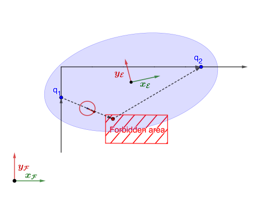
(a) Showcase of a reachability region

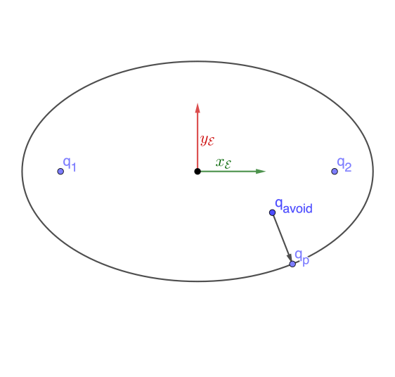
(b) Point-ellipsoid constraint

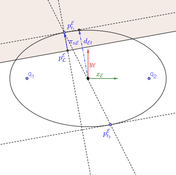
(c) Plane-ellipse constraint

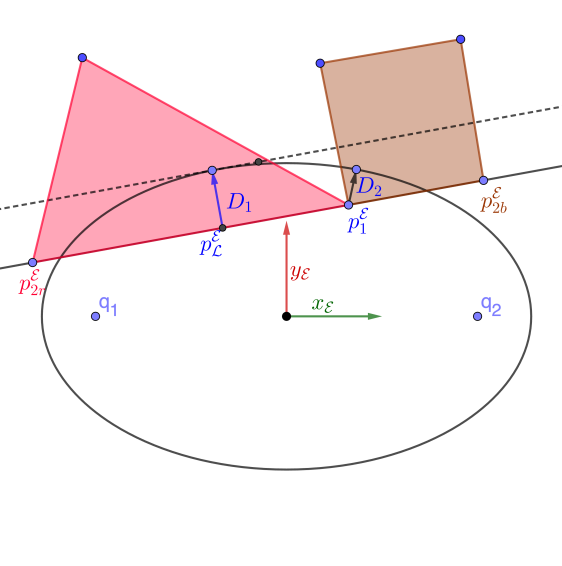
(d) Polygon-ellipse constraint

Figure 2: Figure 2a showcases the ellipsodial reachability region. Black line is the planned trajectory, $q_{1}$ and $q_{2}$ are two co-observed locations the robot are expected at given time $t_{1}$ and $t_{2}$, dashed lines show possible trajectory of a compromised robot during unobserved period. Axis of global frame $\mathcal{F}$ and canonical frame $\mathcal{F}_{\mathcal{E}}$ are shown as $x_{\mathcal{F}},y_{\mathcal{F}}$ and $x_{\mathcal{E}},y_{\mathcal{E}}$ respectively. In Figure 2b, a point $q_{avoid}$ inside ellipsoid is projected to the areas outside the ellipsoid $f_{p}$. In Figure 2c, the projection is simplified to the point-ellipse constraint as projecting a point inside ellipse $p_{L}$ to $p_{t}$ on outside the ellipse. In Figure 2d, this constraint is simplified to either a plane-ellipse constraint $D_{1}$ or a point-ellipse constraint $D_{2}$.

The region $\mathcal{E}(q_{1},q_{2})$ is an ellipsoid with foci at $q_{1},q_{2}$, center $o_{\mathcal{E}}=\frac{1}{2}(q_{1}+q_{2})$, and the major radius equal to $a$. We denote as $c_{\mathcal{E}}=\frac{1}{2}\lVert q_{1}-q_{2}\rVert=\lVert o_{\mathcal{E}}-q_{1}\rVert$ the semi-axis distance from the center to a foci. This reachability ellipsoid is an over-approximation of the exact reachability region in Definition 3.

Expanding upon the concept of co-observation and reachability, Definition 1 can be written as,

Remark 1

A multi-robot trajectory is secured against plan-deviation attacks if there exist a co-observation plan such that the reachability region between each consecutive co-observation does not intersect with any forbidden regions.

II-D Transformation to canonical coordinates

To simplify the problem, we employ a canonical rigid body transformation that repositions the ellipse $\mathcal{E}$ from the global frame $\mathcal{F}$ to a canonical frame $\mathcal{F}_{\mathcal{E}}$, and perform this transformation in a differentiable manner with respect to the two foci serving as waypoints for a robot. The canonical frame $\mathcal{F}_{\mathcal{E}}$ is defined with the origin at the ellipsoid’s center, and the first axis aligned with the foci Figure 2a.

For all reachability ellipsoid constraints, we first solve the problem in the canonical frame $\mathcal{F}_{\mathcal{E}}$, and transform the solutions to the global frame $\mathcal{F}$ using the transformation (15). We parametrize the transformation from $\mathcal{F}$ to $\mathcal{F}_{\mathcal{E}}$ using a rotation $R^{\mathcal{F}}_{\mathcal{E}}$ and a translation $o^{\mathcal{F}}_{\mathcal{E}}$, which, to simplify the notation, we refer to as $R$ and $o$, respectively. The transformation of a point from the frame $\mathcal{F}_{\mathcal{E}}$ to the frame $\mathcal{F}$ and its inverse are given by the rigid body transformations:

$${q^{\mathcal{F}}}=R{q^{\mathcal{E}}}+o,\quad{q^{\mathcal{E}}}=R^{\mathrm{T}}({q^{\mathcal{F}}}-o).$$ (15)

We define $\nu_{\mathcal{F}}$ and $\nu_{\mathcal{E}}$ to represent the $x$-axis unitary vector of $\mathcal{F}_{\mathcal{E}}$ in the frames $\mathcal{F}$ and $\mathcal{F}_{\mathcal{E}}$, respectively. Formally:

$$\nu^{\prime}_{\mathcal{F}} =q_{2}-q_{1}, \nu_{\mathcal{F}} =\frac{\nu^{\prime}_{\mathcal{F}}}{\lVert\nu_{\mathcal{F}}\rVert}, \nu_{\mathcal{E}} =[1,0,0]^{T};$$ (16)

see Fig.2a for an illustration. Note that $\nu_{\mathcal{E}}$ is constant while, for the sake of clarity, $\nu_{\mathcal{F}}$ depends on $q_{1},q_{2}$. From the definition of $\mathcal{F}_{\mathcal{E}}$, the rotation $R$ can be found using a Householder rotation, while from (15) the translation $o$ must be equal to the center of $\mathcal{E}(q_{1},q_{2})$ expressed in $\mathcal{F}$, i.e.:

$$R =H(\nu_{\mathcal{F}}(q_{1},q_{2}),\nu_{\mathcal{E}}(q_{1},q_{2})), o =\frac{1}{2}(q_{1}+q_{2}).$$ (17)

To simplify the notation, in the following, we will consider $H$ to be a function of $q_{1},q_{2}$ directly, i.e. $H(q_{1},q_{2})$. The ellipse $\mathcal{E}$ expressed in $\mathcal{F}_{\mathcal{E}}$ is given by ${\mathcal{E}^{\mathcal{E}}}=\{{q^{\mathcal{E}}}\in m:d(q^{\mathcal{E}}_{1},{q^{\mathcal{E}}})+d({q^{\mathcal{E}}},q^{\mathcal{E}}_{2})<2a\}$, with foci $q^{\mathcal{E}}_{1},q^{\mathcal{E}}_{2}$ in $\mathcal{F}_{\mathcal{E}}$ defined as

$$q^{\mathcal{E}}_{1}=\begin{bmatrix}c&0&0\end{bmatrix}^{\mathrm{T}}, q^{\mathcal{E}}_{2}=\begin{bmatrix}-c&0&0\end{bmatrix}^{\mathrm{T}},$$ (18)

and semi-axis distance $c=\frac{\lVert q_{2}-q_{1}\rVert}{2}$.

Definition 5

The reachability ellipsoid $\mathcal{E}$ in the canonical frame is defined as as the zero level set of the quadratic function

$${E^{\mathcal{E}}}({q^{\mathcal{E}}})={q^{\mathcal{E}}}^{\mathrm{T}}Q{q^{\mathcal{E}}}-1$$ (19)

where

$$Q=\operatorname{diag}(a^{-2},b^{-2},b^{-2}),$$ (20)

and $b=\sqrt{a^{2}-c^{2}}$. The ellipse parameters $a$, $b$ represent the lengths of the major axes.

Lemma 1

The original ellipse $\mathcal{E}$ in $\mathcal{F}$ can be expressed as the zero level set of the quadratic function

$${E^{\mathcal{F}}}({q^{\mathcal{F}}})=({q^{\mathcal{F}}}-o_{\mathcal{E}})^{\mathrm{T}}H^{\mathrm{T}}QH({q^{\mathcal{F}}}-o_{\mathcal{E}})-1$$ (21)

Proof:

The claim follows by substituting (15) into (19), and from the definition of $R$ and $o$. ∎

We are now ready to formulate constraints based on reachability ellipsoids against different types of forbidden regions: a point, a plane, a segment, and a convex polygon which is is done by defining $D(q)$, its differential $\partial_{q}D(q)$, the set $\zeta$ and the projection $\Pi_{\zeta}$.

II-E Point-ellipsoid reachability constraint

As shown in Fig.2b, we consider a forbidden region in the shape of a single point $q_{avoid}$. The goal is to design the trajectory $q(t)$ such that $q_{avoid}\notin\mathcal{E}(q_{1},q_{2})$. This constraint can be written as,

ADMM constraint 2 (Point-ellipsoid reachability constraint)

$$D(\mathbf{q}) =\begin{cases}\pi_{p\mathcal{E}}(\mathbf{q})-q_{avoid}&q_{avoid}\in\mathcal{E},\\ {0}&\textrm{otherwise}.\end{cases}$$ (22)

$$\mathcal{Z} =\{q\in\mathbb{R}^{nm}:\lVert D_{p}(\mathbf{q})\rVert=0\},$$ (23)

$$\Pi_{\mathcal{Z}}(\mathbf{z}) =0,$$ (24)

where $\pi_{p\mathcal{E}}(q_{avoid};q_{1},q_{2},a)=q_{p}$ is a projection function that returns a projected point $q_{p}$ of $q_{avoid}$ outside the ellipse, i.e., as the solution to

$$\pi_{p\mathcal{E}}=\operatorname*{\arg\!\min}_{q_{p}\in\mathcal{E}^{c}}\quad\lVert q_{avoid}-q_{p}\rVert^{2}$$ (25)

where $\mathcal{E}^{c}$ is the set complement of region $\mathcal{E}$.

For cases where $q_{avoid}\notin\mathcal{E}(q(t_{2}),q(t_{1}),r)$, $\pi_{p\mathcal{E}}(q_{avoid})=q_{avoid}$. And for cases where $q_{avoid}\in\mathcal{E}(q_{1},q_{2},r)$, $D(q)$ needs to be projected to the boundary of the ellipse. In the canonical frame $\mathcal{F}_{\mathcal{E}}$, the projected point $q^{\mathcal{E}}_{p}$ can be written as:

$$q^{\mathcal{E}}_{p}={(I+sQ)}^{-1}q^{\mathcal{E}}_{avoid}=Sq^{\mathcal{E}}_{avoid}$$ (26)

where $s$ can be solved as the root of the level set (19):

$${q^{\mathcal{E}}_{p}}^{\mathrm{T}}Qq^{\mathcal{E}}_{p}-1={q^{\mathcal{E}}_{avoid}}^{\mathrm{T}}Q^{\prime}(s)q^{\mathcal{E}}_{avoid}-1=0$$ (27)

where

$$Q^{\prime}(s)=S^{\mathrm{T}}QS=\operatorname{diag}\left(\frac{a^{2}}{(s+a^{2})^{2}},\frac{b^{2}}{(s+b^{2})^{2}},\frac{b^{2}}{(s+b^{2})^{2}}\right)$$ (28)

Detailed methods for computing $s$ can be found in [5, 6, 27].

The point-to-ellipse projection function in $\mathcal{F}$ is then:

$$\pi_{p\mathcal{E}}(q)=R^{-1}(q(t_{1}),q(t_{2}))q^{\mathcal{E}}_{p}+o\\ =R^{-1}(q(t_{1}),q(t_{2}))Sq^{\mathcal{E}}_{avoid}+o\\ =R^{-1}SR(q_{avoid}-o)+o$$ (29)

In our derivations, we consider only the 3-D case ($m=3$); for the 2-D case, let $P=\begin{bmatrix}I&0\end{bmatrix}\in 2\times 3$: then $\pi_{p\mathcal{E}}^{\textrm{2D}}=P\pi_{p\mathcal{E}}^{\textrm{3D}}(P^{\mathrm{T}}q_{avoid};P^{\mathrm{T}}q_{1},P^{\mathrm{T}}q_{2},a)$.

Proposition 3

The differential of the projection operator $\pi_{p\mathcal{E}}(q_{avoid};q_{1},q_{2},a)$ with respect to the foci $q_{1},q_{2}$ is given by the following (using $q$ as a shorthand notation for $q^{\mathcal{E}}_{avoid}$)

$$\partial_{\left[\begin{smallmatrix}q_{1}\\ q_{2}\end{smallmatrix}\right]}\pi_{p\mathcal{E}}=-2H[SH(q-o)]_{\times}U\\ +\left((q^{\mathrm{T}}\partial_{s}Q^{\prime}q)^{-1}H^{-1}Q^{\prime}qq^{\mathrm{T}}(4Q^{\prime}H[q-o]_{\times}U\right.\\ \left.+2Q^{\prime}H\partial_{q}o-\partial_{b}Q^{\prime}qq\partial_{q}b)-sH^{-1}S^{2}\partial_{b}Qq\partial_{q}b\right)\\ -2H^{-1}SH[q-o]_{\times}U+(H^{-1}SH-I)\partial_{q}o$$ (30)

Proof:

See Section -C. ∎

The differential of $D_{p}$ is the same as the one for $\pi_{p\mathcal{E}}$.

II-F Plane-ellipsoid reachability constraint

For forbidden region in the shape of a hyperplane $\mathcal{L}({q^{\mathcal{F}}})=\{{q^{\mathcal{F}}}\in\mathbb{R}^{n}:\mathbf{n}^{\mathrm{T}}{q^{\mathcal{F}}}=d\}$ (as shown in Figure 2c), the reachability constraint can be defined as $\mathcal{L}\cap\mathcal{E}(q_{1},q_{2},a)=\emptyset$. When transformed into the canonical frame, the hyperplane can be written as ${\mathcal{L}^{\mathcal{E}}}({q^{\mathcal{E}}})=\{{q^{\mathcal{E}}}\in\mathbb{R}^{m}:\mathbf{n}_{\mathcal{E}}^{\mathrm{T}}{q^{\mathcal{E}}}=d_{\mathcal{E}}\}$, where,

$$\mathbf{n}_{\mathcal{E}}=H(q_{1},q_{2})\mathbf{n},\quad d_{\mathcal{E}}=-\mathbf{n}^{\mathrm{T}}o+d.$$ (31)

Intuitively, $d_{\mathcal{E}}$ can be thought as a distance between the the plane $\mathcal{L}$ and the origin (i.e., the center of $\mathcal{E}$).

For every ${\mathcal{L}^{\mathcal{E}}}({q^{\mathcal{E}}})$, there always exist two planes that are both parallel to $\mathcal{L}$ and tangential to the ellipse (i.e. resulting in a unique intersection point), $\mathcal{L}_{1}^{\mathcal{E}}=\{{q^{\mathcal{E}}}\in\mathbb{R}^{m}:\mathbf{n}_{\mathcal{E}}^{\mathrm{T}}{q^{\mathcal{E}}}=d_{\mathcal{E}t}\}$ and $\mathcal{L}_{2}^{\mathcal{E}}=\{{q^{\mathcal{E}}}\in\mathbb{R}^{m}:\mathbf{n}_{\mathcal{E}}^{\mathrm{T}}{q^{\mathcal{E}}}=-d_{\mathcal{E}t}\}$ (Figure 2c). And the intersection point can be written as:

$$p^{\mathcal{E}}_{t_{1}}=\frac{d_{\mathcal{E}t}Q^{-1}n_{\mathcal{E}}}{n_{\mathcal{E}}^{\mathrm{T}}Q^{-1}n_{\mathcal{E}}}=\frac{Q^{-1}n_{\mathcal{E}}}{d_{\mathcal{E}t}},\quad p^{\mathcal{E}}_{t_{2}}=-p^{\mathcal{E}}_{t_{1}},$$ (32)

where $d_{\mathcal{E}t}=\sqrt{n_{\mathcal{E}}^{\mathrm{T}}Q^{-1}n_{\mathcal{E}}}$; intuitively, $d_{\mathcal{E}t}$ can be thought as a distance between the tangent plane $\mathcal{L}_{1}^{\mathcal{E}}$ (or $\mathcal{L}_{2}^{\mathcal{E}}$) and the origin (i.e., the center of the ellipse $\mathcal{E}$).

We introduce the concept of a tangent interpolation point on the hyperplane to characterize the relationship between the plane and the ellipse.

Definition 6

The tangent interpolation point $p^{\mathcal{E}}_{\mathcal{L}}\in\mathcal{L}$ is defined on the plane by

$$p^{\mathcal{E}}_{\mathcal{L}}=\frac{d_{\mathcal{E}}Q^{-1}n_{\mathcal{E}}}{n_{\mathcal{E}}^{\mathrm{T}}Q^{-1}n_{\mathcal{E}}}.$$ (33)

Intuitively, the point $p^{\mathcal{E}}_{\mathcal{L}}$ is the point on $\mathcal{L}$ which is closest to either $p^{\mathcal{E}}_{1}$ or $p^{\mathcal{E}}_{2}$. Note that when $d_{\mathcal{E}}=d_{\mathcal{E}t}$ or $d_{\mathcal{E}}=-d_{\mathcal{E}t}$, $p^{\mathcal{E}}_{\mathcal{L}}=p^{\mathcal{E}}_{t_{1}}$ or $p^{\mathcal{E}}_{\mathcal{L}}=p^{\mathcal{E}}_{t_{2}}$, respectively. When $d_{\mathcal{E}}\in[-d_{\mathcal{E}t},d_{\mathcal{E}t}]$, the plane $\mathcal{L}$ and the ellipsoid $\mathcal{E}$ have at least one intersection, thus violating our desired reachability constraint.

With these definitions, the constraint can be written as:

ADMM constraint 3 (Plane-ellipsoid reachability constraint)

$$D(\mathbf{q}) =H^{-1}(q_{1},q_{2})\pi^{\mathcal{E}}_{\mathbf{n}_{\mathcal{E}}}(\mathbf{q})+o,$$ (34)

$$\mathcal{Z} =\{\mathbf{q}\in\mathbb{R}^{nm}:\lVert D_{\mathbf{n}}(\mathbf{q})\rVert=0\},$$ (35)

$$\Pi_{\mathcal{Z}}(\mathbf{z}) =\overrightarrow{0},$$ (36)

where $\pi^{\mathcal{E}}_{\mathbf{n}_{\mathcal{E}}}(q)$ is the projection operator defined as:

$$\pi^{\mathcal{E}}_{\mathbf{n}_{\mathcal{E}}}(\mathbf{q})=\begin{cases}p^{\mathcal{E}}_{t_{1}}-p^{\mathcal{E}}_{\mathcal{L}}&\textrm{ if }d_{\mathcal{E}}\in[0,d_{\mathcal{E}t}],\\ p^{\mathcal{E}}_{t_{2}}-p^{\mathcal{E}}_{\mathcal{L}}&\textrm{ if }d_{\mathcal{E}}\in[-d_{\mathcal{E}t},0),\\ {0}&\textrm{otherwise}.\end{cases}$$ (37)

Proposition 4

The differential of the projection function $\pi^{\mathcal{E}}_{\mathbf{n}\mathcal{E}}(\mathbf{q})$ with respect to the foci $q_{1}$ and $q_{2}$ is given by:

$$\partial_{q}\pi^{\mathcal{E}}_{\mathbf{n}\mathcal{E}}(q)=\begin{cases}\partial_{q}p^{\mathcal{E}}_{t1}-\partial_{q}p^{\mathcal{E}}_{\mathcal{L}}&d_{\mathcal{E}}\in[0,d_{\mathcal{E}t}],\\ \partial_{q}p^{\mathcal{E}}_{t2}-\partial_{q}p^{\mathcal{E}}_{\mathcal{L}}&d\in[-d_{\mathcal{E}t},0),\\ {0}&otherwise.\end{cases}$$ (38)

where

$$\partial_{q}p_{\mathcal{L}}=(-\frac{d_{\mathcal{E}t}n^{\mathrm{T}}\partial_{q}o-2d_{\mathcal{E}}\partial_{q}d_{\mathcal{E}t}}{d_{\mathcal{E}t}^{3}})Q^{-1}n_{\mathcal{E}}\\ +\frac{d_{\mathcal{E}}\partial_{b}Q^{-1}n_{\mathcal{E}}\partial_{q}b-2d_{\mathcal{E}}Q^{-1}H[n]_{\times}U}{d_{\mathcal{E}t}^{2}},$$ (39)

$$\partial_{q}p_{1}=-\frac{Q^{-1}n_{\mathcal{E}}\partial_{q}d_{\mathcal{E}t}}{d_{\mathcal{E}t}^{2}}+\frac{\partial_{b}Q^{-1}n_{\mathcal{E}}\partial_{q}b-2Q^{-1}H[n]_{\times}U}{d_{\mathcal{E}t}}.$$ (40)

Proof:

See Section -D. ∎

Based on the Proposition 4, the differential of (34) can be written as:

$$\partial_{q}{D_{\mathbf{n}\mathcal{E}}}=-2H[{\Pi^{\mathcal{E}}}_{\mathbf{n}\mathcal{E}}]_{\times}\!M+H^{-1}\partial_{q}{\Pi^{\mathcal{E}}}_{\mathbf{n}\mathcal{E}}$$ (41)

II-G Line-segment-ellipse reachability constraint

For a intermediate step to get the relationship between a polygon shaped forbidden region, the relative position between the ellipse and segment of the hyperplane that defines the region is studied. Assume the segment on hyperplane ${\mathcal{L}^{\mathcal{E}}}({q^{\mathcal{E}}})=\{{q^{\mathcal{E}}}\in\mathbb{R}^{m}:\mathbf{n}_{\mathcal{E}}^{\mathrm{T}}{q^{\mathcal{E}}}=d_{\mathcal{E}}\}$ has endpoints ${p_{1}^{\mathcal{E}}}$ and ${p_{2}^{\mathcal{E}}}$; then the segment can be defined as:

$$\begin{bmatrix}({p_{1}^{\mathcal{E}}}-{p_{2}^{\mathcal{E}}})^{\mathrm{T}}\\ ({p_{2}^{\mathcal{E}}}-{p_{1}^{\mathcal{E}}})^{\mathrm{T}}\end{bmatrix}{p^{\mathcal{E}}}\leq\begin{bmatrix}{p_{2}^{\mathcal{E}}}^{\mathrm{T}}\\ -{p_{1}^{\mathcal{E}}}^{\mathrm{T}}\end{bmatrix}({p_{1}^{\mathcal{E}}}-{p_{2}^{\mathcal{E}}}),\quad\mathbf{n}_{\mathcal{E}}^{\mathrm{T}}{q^{\mathcal{E}}}=d_{\mathcal{E}}.$$ (42)

For cases, where the tangent interpolation point ${p_{\mathcal{L}}^{\mathcal{E}}}$ stays within the segment (i.e. red region in Figure 2d, where ${p_{\mathcal{L}}^{\mathcal{E}}}$ lies between ${p_{1}^{\mathcal{E}}}$ and ${p_{2r}^{\mathcal{E}}}$), the constraint can be seen as a plane-ellipse constraint in Section II-F. Otherwise (i.e. brown region in Figure 2d, where ${p_{\mathcal{L}}^{\mathcal{E}}}$ lies outside ${p_{1}^{\mathcal{E}}}$ and ${p_{2b}^{\mathcal{E}}}$), the constraint can be seen as a point-ellipse constraint in Section II-E.

ADMM constraint 4 (Line-segment-ellipsoid reachability constraint)

$$D(\mathbf{q}) =\begin{cases}D_{p_{1}}(\mathbf{q})&({p_{1}^{\mathcal{E}}}-{p_{2}^{\mathcal{E}}})^{\mathrm{T}}({p_{\mathcal{L}}^{\mathcal{E}}}-{p_{2}^{\mathcal{E}}})<0\\ D_{p_{2}}(\mathbf{q})&({p_{2}^{\mathcal{E}}}-{p_{1}^{\mathcal{E}}})^{\mathrm{T}}({p_{\mathcal{L}}^{\mathcal{E}}}-{p_{1}^{\mathcal{E}}})<0\\ D_{p_{\mathcal{L}}^{\mathcal{E}}}(\mathbf{q})&\textrm{otherwise}\end{cases}$$ (43)

$$\mathcal{Z} =\{\mathbf{q}\in\mathbb{R}^{nm}:\lVert D(\mathbf{q})\rVert=0\},$$ (44)

$$\Pi_{\mathcal{Z}}(\mathbf{z}) =0,$$ (45)

where $D_{p_{1}}$ and $D_{p_{2}}$ are the point-ellipsoid constraint projection function with respect to ${p_{1}^{\mathcal{E}}}$ and ${p_{2}^{\mathcal{E}}}$ in (22), and $D_{p_{\mathcal{L}}^{\mathcal{E}}}$ is the plane-ellipsoid constraint with respect to frame ${\mathcal{L}^{\mathcal{E}}}$ in (34).

II-H Convex-polygon-ellipse reachability constraint

To keep an ellipse away from a convex polygon, first, we need to keep all segments of the hyperplanes outside the ellipse. Similar to (33), we define

ADMM constraint 5 (Convex-polygon-ellipsoid reachability constraint)

$$D(\mathbf{q}) =\begin{bmatrix}D_{seg1}(\mathbf{q})\\ D_{seg2}(\mathbf{q})\\ \vdots\end{bmatrix}$$ (46)

$$\mathcal{Z} =\{\mathbf{q}\in\mathbb{R}^{nm}:\lVert D(\mathbf{q})\rVert=0\},$$ (47)

$$\Pi_{\mathcal{Z}}(\mathbf{z}) =0,$$ (48)

where $D_{seg}$ are the constraint functions for each line segment used to define convex polygon region. ADMM constraint 5 needs to be supplemented with a convex obstacle constraint for the polygon (as introduced in [6]) to prevent cases where the ellipse is a subset of the region.

II-I Secured planning results and limitation

We test the newly introduced security constraints to a map exploration problem, illustrated in Figure 3 in both simulations and on an experimental testbed, involving a 3-robot system assigned to explore a $10m\times 10m$ region with one obstacle, Zone 1, and two forbidden zones, Zone 2 and Zone 3. The maximum velocity constraint $v_{max}=0.5m/dt$, time horizon $T=20$.

We employ the APMAPF solver ([2]) to generate a MAPF plan with a co-observation schedule in a grid-world application (Fig.3a). This result serves as the initial trajectory input for the ADMM solver. This obtained plan is then transformed to a continuous configuration space, addressing map exploration tasks. Co-observation schedules are set up using the APMAPF algorithm for two forbidden regions. Reachability constraints are added to ensure an empty intersection between all robots’ reachability regions during co-observations and the forbidden regions. It’s important to note that the secured attack-proof solution is initially infeasible in the continues setting, unless additional checkpoints (e.g., stationary security cameras) are incorporated (additional task added for agent 3 to visit the checkpoint at time $8$). Further solutions to avoid these checkpoints are discussed in Section III.

The simulation result, shown in Fig. 3c, displays reachability regions as black ellipsoids, demonstrating empty intersections with Zones 2 and 3. Explicit constraints between reachability regions and obstacles are not activated, assuming basic obstacle avoidance capabilities in robots. The intersections between obstacles and ellipsoids, as observed between agent 3 and Zone 1, are deemed tolerable. All constraints are satisfied, and agents have effectively spread across the map for optimal exploration tasks.

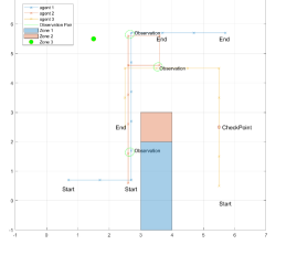
(a) Grid-world trajectory.

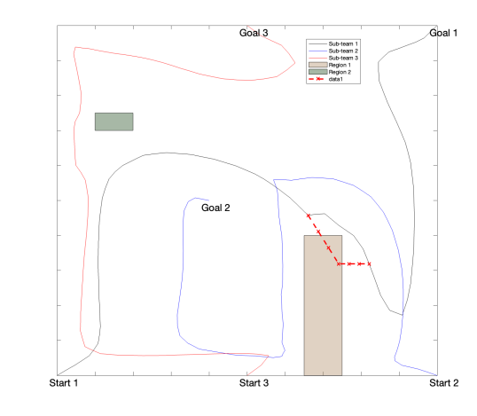
(b) Continuous world trajectory

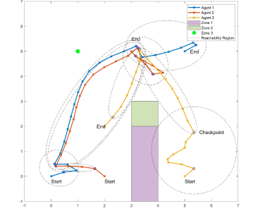
(c) Securd result

Figure 3: Trajectory design of an example map exploration task for a three-robot system with start locations and destinations fixed. Task are planned in a $8\times 8$ grid world. Zone 1 is obstacle, Zone 2 and Zone 3 are safe zones. Figure 3a shows the planned trajectory with co-observation schedule in grid-world. Figure 3b shows the unsecured trajectory design in continuous world optimized with respect to a map exploration task where Zone 1 and 2 are considered together as one obstacle. A potential path that could break the security by entering region 1 is highlighted in dashline. Figure 3c shows the secured trajectory with the incorporation of co-observation and reachability constraints.

II-I1 Limitations

Our solution demonstrates the potential of planning with reachability and co-observation to enhance the security of multi-agent systems. However, two primary challenges need to be addressed. Firstly, achieving a co-observation and reachability-secured plan may not always be feasible when robots are separated by obstacles or forbidden regions, making it impossible for them to establish co-observation schedules or find a reachability-secured path. For example, Agent 3 in Figure 3c required an additional security checkpoint to create secured reachability areas. Secondly, meeting security requirements may impact overall system performance, as illustrated by the comparison between Figure 3b and 3c. The introduction of security constraints led to the top left corner being unexplored by any robots. This trade-off between security and system performance is particularly significant given that system performance plays a crucial role in the decision to employ multi-agent systems. These challenges are addressed in Chapter III to ensure the effective use of planning with reachability and co-observation in securing multi-agent systems.

III Cross-trajectory co-observation planning

To address the feasibility and performance trade-offs, we propose to form sub-teams on each route, and setup additional co-observations both within the sub-team and across different sub-teams. These cross-trajectory co-observations allow sub-teams to obtain trajectories that are closer to the optimal (as shown in Figure 1), because they do not require the entire sub-team to meet with other teams for co-observations, thus providing more flexibility.

III-A Problem overview

We start with an unsecured MRS trajectory with $n_{p}$ routes $\{q_{p}\}_{p=1}^{N_{p}}$ (the ADMM-based planner in Section II without security constraints is used, but other planners are applicable). Here, the state $q_{p}(t),p\in\{\mathcal{I}_{0},\ldots,\mathcal{I}_{p}\}$ represents the reference position of the $i$-th sub-team at time $t\in\{0,\dots,T\}$. Introducing redundant robots into the MRS, we assume a total of $n>n_{p}$ robots are available and organized into sub-teams through a time-varying partition $\mathcal{I}(t)=\cup_{p}\mathcal{I}_{p}(t)$ where robots in each sub-team $\mathcal{I}_{p}$ share the same nominal trajectory. To ensure the fulfillment of essential tasks, at least one robot is assigned to adhere to the reference trajectory. The remaining redundant $n_{p}-n$ robots are strategically utilized to enhance security. These robots focus on co-observations either within their respective sub-teams, or when necessary, deviate and join another sub-team to provide necessary co-observations. The objective of this problem is to formulate a strategy for this new co-observation strategy, named cross-trajectory co-observation that the resulting MRS plan meet the security in Remark 1 while minimizing the number of additional robots required.

We model the planned trajectory $\{q_{p}\}_{p=1}^{N_{p}}$ as a directed checkpoint graph $G{q}=(V_{q},E_{q})$, where vertices $V_{q}$ represent key locations requiring co-observation (as required by Remark 1), and edges $E_{q}=E_{t}\cup E_{c}$ connect pairs of vertices if possible paths exist. Inspired by [8], additional robots in the sub-team are treated as flows in the checkpoint graph. This transforms the co-observation planning problem into a network multi-flow problem, solvable with general Mixed-Integer Linear Programming techniques.

This section presents the two components of our approach: constructing the checkpoint graph based on unsecured multi-robot trajectories, and the formulation and solution of the network multi-flow problem.

III-B Rapidly-exploring Random Trees

To find edges between different nominal trajectories, we use the $\texttt{RRT}^{\texttt{*}}$ [28] algorithm to find paths from a waypoint on one trajectory to multiple destination points (i.e., reference trajectories of other sub-teams, in our method). As a optimal path planning algorithm, $\texttt{RRT}^{\texttt{*}}$ returns the shortest paths between an initial location and points in the free configuration space, organized as a tree. We assume that the generated paths can be travelled in both directions (this is used later in our analysis). Key functions from $\texttt{RRT}^{\texttt{*}}$ that are also used during constructions of the checkpoint graph are

$\texttt{Cost}(v)$

This function assigns a non-negative cost (total travel distance in our application) to the unique path from the initial position to $v$ .

$\texttt{Parent}(v)$

This is a function that maps the vertex $v$ to $v^{\prime}\in V$ such that $(v^{\prime},v)\in E$.

Our objective here is to ascertain the existence of feasible paths instead of optimize specific tasks. While the ADMM based solver Section II presented earlier offers a broader range of constraint handling, RRT*’s efficient exploration of the solution space, coupled with its ability to incorporate obstacle constraints, makes it a fitting choice for building the checkpoint graph.

III-C Checkpoint graph construction

In this section, we define and search for security checkpoints and how to use $\texttt{RRT}^{\texttt{*}}$ to construct the checkpoint graph $G_{q}$.

III-C1 Checkpoints

Let $q_{p}\in nT$ represent the trajectory for sub-team $p$ with time horizon $T$, where $q_{p}(t)\in n$ denotes the reference waypoint at time $t$. We identify checkpoints within $q_{p}$ that require co-observations for securty, as outlined in Remark 1. Checkpoint $v_{pi}=(q_{pi},t_{i})$ signifies a required co-observation for sub-team $p$, defined by a location $q_{pi}=q_{p}(t_{i})$ and time $t_{i}$. For simplicity, let $\mathcal{I}_{v_{i}}$ denote the sub-team to which $v_{i}$ belongs, and $q_{v_{pi}}=q_{pi}$ and $t_{v_{pi}}$ be the corresponding waypoint and time for checkpoint $v_{pi}$. To ensure the security of the reference trajectory, the reachability region between consecutive checkpoints must avoid intersections with forbidden areas. This requirement can be formally stated as:

Remark 2

A set of checkpoints $V_{p}=\{v_{p0},\dots,v_{pT}\}$ (arranged in ascending order of $t_{v_{pi}}$) can secure the reference trajectory for sub-team $p$, if $\mathcal{E}(q_{v_{pi}},q_{v_{p(i+1)}},t_{v_{pi}},t_{v_{p(i+1)}})\cap F=\emptyset$ for every $i$, where $F$ is the union of all forbidden areas.

A heuristic approach is provided (Algorithm 1) to locate the checkpoints on given trajectories (an optimal solution would likely be NP-hard, while the approach below works well enough for our purpose).

Algorithm 1 Secure Checkpoint Generate for sub-team $p$

$v_{p0}\leftarrow(q_{p}(0),0)$; $v_{pT}\leftarrow(q_{p}(T),T)$

$V_{p}=\{v_{p0},v_{pT}\}$

$t_{0}\leftarrow 0$; $t_{1}\leftarrow T$

while $\mathcal{E}(q_{p}(t_{0}),q_{p}(t_{1}),t_{0},t_{1})\cap F\neq\emptyset$ or $t_{1}-t_{0}>1$ do

     $i\leftarrow 1$; $j\leftarrow 1$

     while $\mathcal{E}(q_{p}(t_{0}),q_{p}(t_{0}+i),t_{0},t_{0}+i)\cap F=\emptyset$ and $t_{0}+i>t_{1}$ do

         $v_{pf}\leftarrow(q_{p}(t_{0}+i),t_{0}+i)$

         $i\leftarrow i+1$

     end while

     $V_{p}\leftarrow V_{p}\cup v_{pf}$

     while $\mathcal{E}(q_{p}(t_{1}-j),q_{p}(t_{1}),t_{1}-j,t_{1})\cap F=\emptyset$ and $t_{0}+i\geq t_{1}-j$ do

         $v_{pb}\leftarrow(q_{p}(t_{1}-j),t_{1}-j)$

         $j\leftarrow j+1$

     end while

     if $t_{0}+i\neq t_{1}-j$ then

         $V_{p}\leftarrow V_{p}\cup v_{pb}$

     end if

end while

III-C2 Cross-trajectory edges

To enable co-observation cross different sub-team at checkpoints, we search for available connection paths (cross-trajectory edges) between checkpoints on different trajectories, allowing robots deviate from one sub-team to perform co-observation with a different sub-team.

Cross-trajectory edges $E_{c}=(v_{1},v_{2})$ define viable paths between two reference trajectories, where $\mathcal{I}_{v_{1}}\neq\mathcal{I}_{v_{2}}$ and at least one of $v_{1}$ and $v_{2}$ correspond to a security checkpoint $\cup_{p}V_{p}$. The cross-trajectory edges must also adhere to reachability constraints $\mathcal{E}(q_{v_{1}},q_{v_{2}},t_{v_{1}},t_{v_{2}})\cap F=\emptyset$ to ensure that no deviations into forbidden areas can occur during trajectory switches.

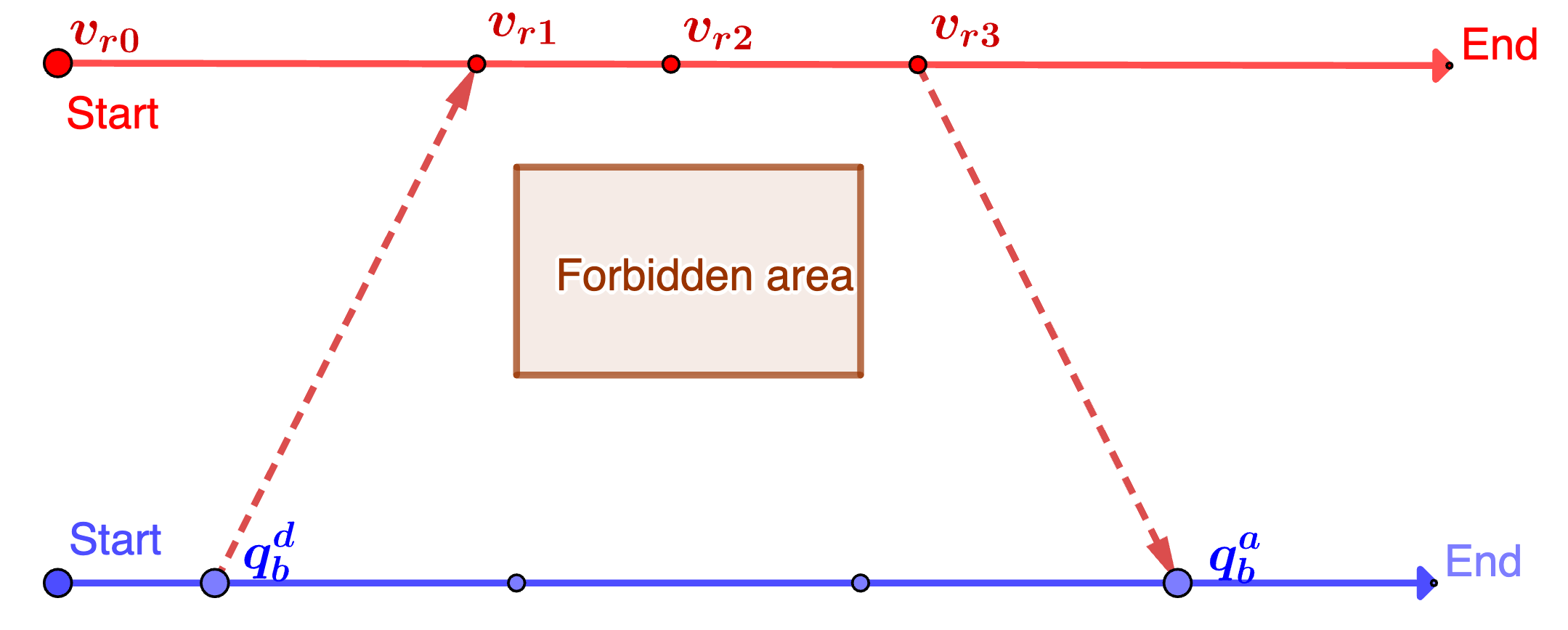
(a) Cross-trajectory edge generation

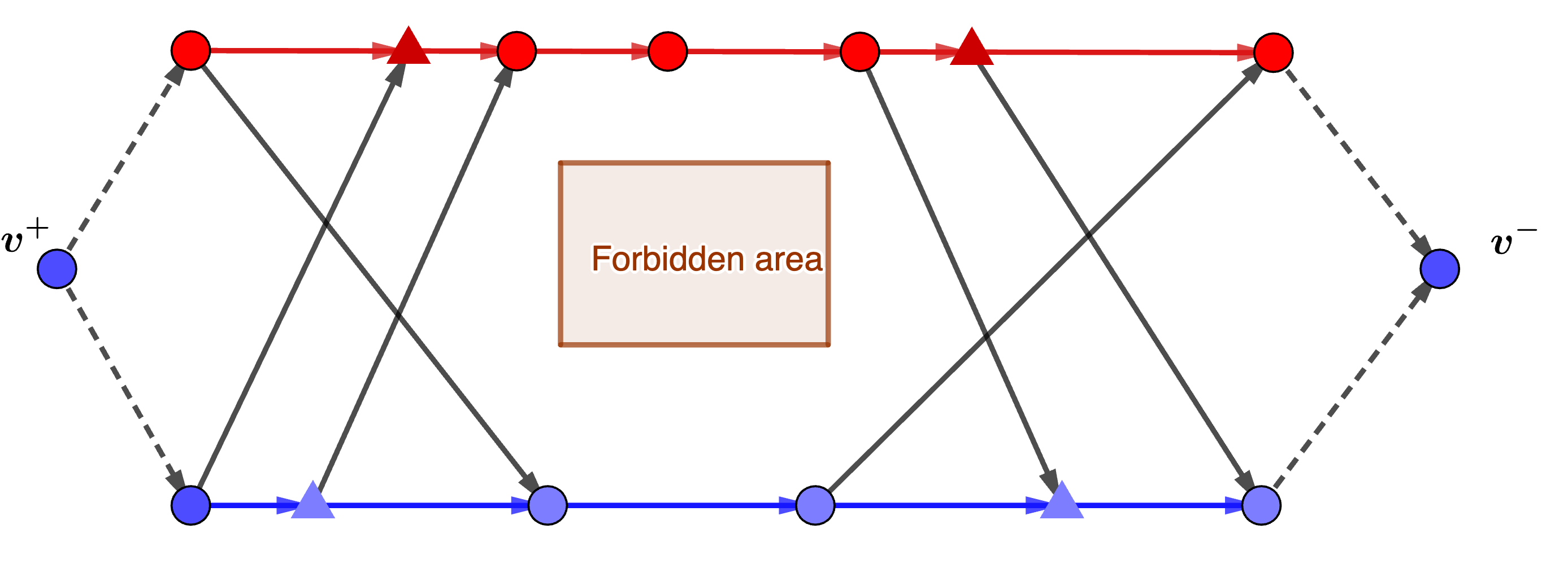
(b) Full checkpoint graph

Figure 4: Figure 4a, Latest departure node $q^{d}_{b}$ found for $v_{r1}$ and earliest arrival node $q^{a}_{b}$ found for $v_{r3}$. Figure 4b, example of a full checkpoint graph where round vertices are checkpoint generated through the heuristic search and triangle vertices are added with the cross-trajectory edges. Virtual source $v^{+}$ and sink $v^{-}$ are added to be used later in planning problem.

We first find trees of feasible paths between each security checkpoint and all other trajectories using position information alone (ignoring, for the moment, any timing constraint). More precisely, through $\texttt{RRT}^{\texttt{*}}$, we find all feasible, quasi-optimal paths between one security checkpoint location $q_{v_{p}}(t_{v_{p}})$ where $v_{p}\in V_{p}$ for sub-team $\mathcal{I}_{p}$, and all the waypoints $\{q_{r}(t_{{r}_{i}})\}$ on any reference trajectory for a different sub-team $\mathcal{I}_{r}$. Then, to prune these trees, we consider the time needed to physically travel from one trajectory to the other while meeting other robots at the two endpoints. This is done by calculating the minimal travel time $t_{\textrm{path}}=\texttt{Cost}(q)/v_{max}$ for a robot to traverse each path. Two types of connecting nodes can be found.

Arrival nodes

are waypoints on $\{q_{r}\}$ where robots from sub-team $\mathcal{I}_{p}$, deviating at $v_{p}$, can meet with sub-team $\mathcal{I}_{r}$ at $(q_{r}(t_{r_{i}}),t_{r_{i}})$. For these, $\texttt{RRT}^{\texttt{*}}$ must have found a path from $v_{p}$ to $q_{r}(t^{a}_{r})$ with $t_{p}+t_{\textrm{path}}<t_{{r}_{i}}$, and $\mathcal{E}(q_{r}(t_{{r}_{i}}),q_{p},t_{{r}_{i}},t_{p})\cap F=\emptyset$.

For each trajectory $r\neq p$, we define the earliest arrival node from $v_{p}$ to $v_{ea}=(q_{r}(t^{a}_{r}),t^{a}_{r})$ as the arrival node characterized by the minimum $t^{a}_{r}$ discovered.

Departure nodes

are the waypoints on $\{q_{r}\}$ such that a robot from sub-team $\mathcal{I}_{r}$, deviating from $(q_{r}(t_{{r}_{i}}),t_{{r}_{i}})$, can meet with robots in sub-team $\mathcal{I}_{p}$ at $v_{p}$. For these nodes, $\texttt{RRT}^{\texttt{*}}$ must find a path from $v_{p}$ to $q_{r}(t_{{r}_{i}})$ for $v_{p}$ if $t_{p}>t_{{r}_{i}}+t_{\textrm{path}}$ and $\mathcal{E}(q_{p},q_{r}(t_{{r}_{i}}),t_{p},t_{{r}_{i}})\cap F=\emptyset$.

For each trajectory $r\neq p$, we define the latest departure node $v_{ld}=(q_{r}(t^{d}_{r}),t^{d}_{r})$ as the departure node characterized by the maximum $t^{d}_{r}$ discovered.

For each $v_{p}\in V_{p}$ found through Algorithm 1, all the latest departure and earliest arrival nodes are added as vertices $V_{q}=V_{p}\cup\{v_{ea},v_{ld}\}$, and the corresponding paths are added as cross-trajectory edges to $E_{q}$. Examples are shown in Figure 4a.

III-C3 In-trajectory edges

We arrange all $V_{q}=\cup_{p}\{v^{0}_{p},\dots,v^{T}_{p}\}$ found in Sections III-C1 and III-C2 in ascending order of $t_{v^{i}_{p}}$. We then add to $E_{q}$ the in-trajectory edges $\{(v^{i}_{p}\rightarrow v^{i+1}_{p})\}$ obtained by connecting all consecutive checkpoints $v^{i}_{p}\in V_{q}$ with the checkpoints $v^{i+1}_{p}$ that follow them in their original trajectories. Examples are shown in Figure 4b.

III-D Co-observation planning problem

In this section, we formulate the cross-trajectory planning problem as a network multi-flow problem, and solve it using mixed-integer linear programs (MILP). We assume that $n_{p}$ robots are dedicated (one in each sub-team) to follow the reference trajectory (named reference robots). The goal is to plan the routes of the $n-n_{p}$ additional cross-trajectory robots dedicated to cross-trajectory co-observations, and potentially minimize the number of ross-trajectory robots needed.

Remark 3

Note that we assign fixed roles to robots for convenience in explaining the multi-flow formulation. In practice, after a cross-trajectory robot joins a team, it is considered interchangable, and could switch roles with the reference robot of that trajectory.

To formulate the problem as a network multi-flow problem, we augment the checkpoint graph $G_{q}$ to a flow graph $G=(V,E)$. The vertices of the new graph $G$ are defined as $V=V_{q}\cup\{v^{+},v^{-}\}$, where $v^{+}$ is a virtual source node, and $v^{-}$ is a virtual sink node. We add directed edges from $v^{+}$ to all the start vertices, and from all end vertices to $v^{-}$, with $v^{0}_{p}$ and $v^{T}_{p}$ representing the start and end vertices of sub-team $\mathcal{I}_{p}$. The edges of the new graph are defined as $E=E_{q}\cup\{(v_{+},v^{0}_{p})\}_{p}\cup\{(v^{T}_{p},v_{-})\}_{p}$.

The path of a robot $k$ all starts from $v^{+}$ and ends at $v^{-}$, and are represented as a flow vector $\mathbf{f}^{k}=\{f^{k}_{ij}\}$, where $f^{k}_{ij}\in\{1,0\}$ is an indicator variable representing whether robot $k$’s path contains the edge $v_{i}\to v_{j}$. The planning problem can be formulated as a path cover problem on $G_{q}$, i.e., as finding a set of paths $F=[\mathbf{f}_{1},\dots,\mathbf{f}_{\mathcal{K}}]$ for cross-trajectory robots such that every checkpoint in $\cup_{p}V_{p}$ is included in at least one path in $F$ (to ensure co-observation at every checkpoint as required by Remark 1).

Technically, we can always create a trivial schedule that involves only co-observations between members of the same team; this, however, would make the solution more vulnerable in the case where multiple agents are compromised in the same team. While in this paper we explicitly consider only the single attacker scenario, multi-attacks can be potentially handled by taking advantage of the decentralized blocklist protocol introduced in [3]. For this reason, we setup the methods presented below to always prefer cross-trajectory co-observation when feasible.

Finally, edges from the virtual source and to the virtual sink should have zero cost, to allow robots to automatically get assigned to the starting point that is most convenient for the overall solution (lower cost when taking cross-trajectory edges). These requirements are achieved with the weights for edges $(v_{i},v_{j})\in E$ defined as:

$$w_{i,j}=\begin{cases}-w_{t}&\mathcal{I}_{v_{i}}=\mathcal{I}_{v_{j}},(v_{i},v_{j})\in E_{q}\\ w_{c}&\mathcal{I}_{v_{i}}\neq\mathcal{I}_{v_{j}},(v_{i},v_{j})\in E_{q}\\ 0&(v_{i},v_{j})\in E/E_{q}\end{cases}$$ (49)

where $w_{c}>w_{t}$.

With the formulation, the planning problem is written as an optimization problem, where the optimization cost balances between the co-observation performance and total number of flows (cross-trajectory robots) needed:

$$\min_{F} \sum^{\mathcal{K}}_{k}\sum_{(+i)\in E}f^{k}_{+i}-\rho\sum^{\mathcal{K}}_{k}\sum_{(ij)\in E}w_{ij}f^{k}_{ij}$$ (50a)

$$s.t. \sum_{\{h:(hi)\in E\}}f^{k}_{hi}=\sum_{\{j:(ij)\in E\}}f^{k}_{ij},\forall k,\forall v\in V_{q}/\{v^{+},v^{-}\}$$ (50b)

$$\sum^{\mathcal{K}}_{k}\sum_{\{i:(ij)\in E\}}f^{k}_{ij}\geq 1,\forall v_{j}\in\{V^{s}_{p}\}$$ (50c)

$$f^{k}_{ij}\in\{0,1\}\,\forall(ij)\in E$$ (50d)

where, for convenience, we used $(ij)$ to represent the edge $(v_{i},v_{j})$, and $(+i)$ to represent the edge $(v^{+},v_{i})$.

The first term in the cost (50a) represents the total number of robot used, and the second term represents the overall co-observation performance (defined as the total number of cross-trajectory edges taken by all flows beyond the regular trajectory edges); the constant $\rho$ is a manually selected penalty parameter to balance between the two terms. (50b) is the flow conservation constraint to ensures that the amount of flow entering and leaving a given node $v$ is equal (except for $v^{+}$ and $v^{-}$). (50c) is the flow coverage constraints to ensures that all security checkpoints $\{V^{s}_{p}\}$ have been visited co-observed. The security graph $G_{q}$ is acyclic, making this problem in complexity class $P$, thus, can be solved in polynominal time [29].

III-E Co-observation performance

Notice that problem (50) is guaranteed to have a solution for $\mathcal{K}=N_{p}$ where all $\mathcal{K}$ robots follows the reference trajectory ($f^{k}_{ij}=1,\forall\mathcal{I}_{v_{i}}=\mathcal{I}_{v_{j}}=k$). It is possible for the resulting flows to have a subset of flows $F_{e}\in F$ that is empty, i.e. $f_{ij}=0,\forall(v_{i},v_{j})\in E$, $f\in F_{e}$; these flow will not increase the cost and can be discarded from the solution.

The constant $\rho$ selects the trade-off between the number of surveillance robots and security performance. An increase in robots generally enhancing security via cross-trajectory co-observations; this also increases the complexity of the coordination across robots. In order to identify the minimum number of robots necessary, we propose an iterative approach where we start with $\mathcal{K}=1$ and gradually increases it until $F$ contains an empty flow, indicating the point where further robot additions do not improve performance.

Remark 4

The value of row $\rho$ is upper bounded such that the second term for each single flow in (50a) is always smaller than one, i.e., $\rho\sum_{(ij)\in E}w_{ij}f^{k}_{ij}\leq 1$. Otherwise, the iteration continues indefinitely as adding additional flow introduce a negative term $\sum_{(+i)\in E}f^{k}_{+i}-\rho\sum_{(ij)\in E}w_{ij}f^{k}_{ij}=1-\rho\sum_{(ij)\in E}w_{ij}f^{k}_{ij}<0$ which always makes the cost (50a) smaller.

III-F Result and simulation

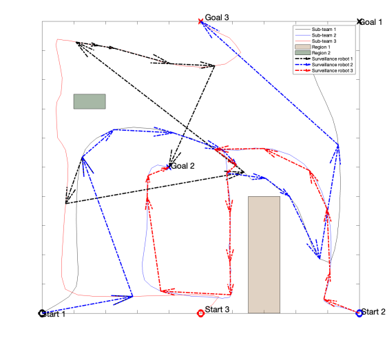
(a) Cross-trajectory co-observation plan

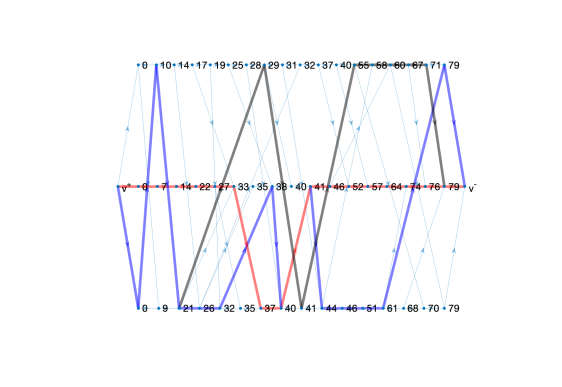
(b) Checkpoint graph and result flows

Figure 5: Figure 5a showcase an unsecured 4-robot map exploration task. The cross-trajectory co-observation plan is shown as dotted arrors on top of the original plan in Figure 5a. The checkpoint graph and resulting flows are shown in Figure 5b.

We first test the proposed method for the example application in Figures 3 and 3c, using the same setup in Section II-I. Using the parameters $w_{c}=10$, $w_{t}=1$ and $\rho=0.01$, the result returns a total of $\mathcal{K}=3$ surveillance robots with cross-trajectory plan shown in Figure 5. The flows derived from the solution of the optimization problem (50) are highlighted in the graph Figure 5b, where each horizontal line represents the original trajectory of a sub-team and the number on each vertex $v_{i}$ represents the corresponding time $t_{i}$. The planning result in the workspace is shown in Figure 5a as dash-dotted arrows with the same color used for each flow in Figure 5b. Compared with the result in Figure 3c, it is easy to see that there is a significant improvement in map coverage in Figure 5a. At the same time, unsecured deviations to the forbidden regions of robots are secured through cross-trajectory observations.

The problem shows no solution for $\mathcal{K}\leq 2$. For cases $\mathcal{K}=3$, problem return the optimal result as shown in Figure 6. If we further increase $\mathcal{K}>3$, we do not get a better result; instead, the planner will return four flows with the rest $\mathcal{K}-3$ flows empty.

We then test the proposed method for a 4-team and 7-team case with result shown in Figure 6, where four trajectories are provided for a map exploration task with no security related constraints (co-observation schedule and reachability). We have a $10m\times 10m$ task space, three forbidden regions (rectangle regions in Figure 6a) and robots with a max velocity of $0.5m/dt$.

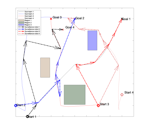
(a) 4-agent co-observation plan

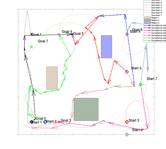
(b) 7-agent co-observation plan

Figure 6: Cross-trajectory co-observation result of a 4 sub-teams task (Figure 6a) and a 7 sub-teams task Figure 6b

IV Summary

This paper introduces security measures for protecting Multi-Robot Systems (MRS) from plan-deviation attacks. We establish a mutual observation schedule to ensure that any deviations into forbidden regions break the schedule, triggering detection. Co-observation requirements and reachability analysis are incorporated into the trajectory planning phase, formulated as constraints for the optimal problem. In scenarios where a secured plan is infeasible or enhanced task performance is necessary, we propose using redundant robots for cross-trajectory co-observations, offering the same security guarantees against plan-deviation attacks. However, the time-sensitive and proximity-dependent nature of co-observation necessitates a focus on collision avoidance during planning. Future work will integrate collision avoidance and explore dynamic duty assignments within sub-teams, increasing the challenge for potential attackers.

-A Proof of proposition 1

For subclaim 1a:

$$H^{\mathrm{T}}H=H^{2}=4uu^{\mathrm{T}}uu^{\mathrm{T}}-4uu^{\mathrm{T}}+I^{2}=I,$$ (51)

since $u^{\mathrm{T}}u=1$.

For subclaim 1b, let $U=\begin{bmatrix}u&u^{\bot}_{1},u^{\bot}_{2}\end{bmatrix}$, where $u^{\bot}_{1},u^{\bot}_{2}$ are two orthonormal vectors such that $I=UU^{\mathrm{T}}=uu^{\mathrm{T}}+u^{\bot}_{1}(u^{\bot}_{1})^{\mathrm{T}}+u^{\bot}_{2}(u^{\bot}_{2})^{\mathrm{T}}$; then, substituting $I$ in (4), we have that the eigenvalue decomposition of $H$ is given by

$$H=U\operatorname{diag}(1,-1,-1)U^{\mathrm{T}}.$$ (52)

Since the determinant of a matrix is equal to the product of the eigenvalues, $\det(H)=1$.

For subclaim 2, first note that $Hu=2uu^{\mathrm{T}}u-u=u$. It follows that the sum of $\nu_{\mathcal{F}}$ and $\nu_{\mathcal{E}}$ is invariant under $H$:

$$H(\nu_{\mathcal{F}}+\nu_{\mathcal{E}})=Hu\lVert\nu_{\mathcal{F}}+\nu_{\mathcal{E}}\rVert=u\lVert\nu_{\mathcal{F}}+\nu_{\mathcal{E}}\rVert=\nu_{\mathcal{F}}+\nu_{\mathcal{E}},$$ (53)

and that their difference is flipped under $H$:

$$H(\nu_{\mathcal{F}}-\nu_{\mathcal{E}})=2uu^{\mathrm{T}}(\nu_{\mathcal{F}}-\nu_{\mathcal{E}})-(\nu_{\mathcal{F}}-\nu_{\mathcal{E}})^{2}=-(\nu_{\mathcal{F}}-\nu_{\mathcal{E}}).$$ (54)

Combining (53) and (54) we obtain

$$H\nu_{\mathcal{F}}=\frac{1}{2}\bigl{(}H(\nu_{\mathcal{F}}+\nu_{\mathcal{E}})+H(\nu_{\mathcal{F}}-\nu_{\mathcal{E}})\bigr{)}=\nu_{\mathcal{E}}$$ (55)

-B Proof or proposition 2

From the definition of $H$ in (4), we have

$$\dot{H}=2(\dot{u}u^{\mathrm{T}}+u\dot{u}^{\mathrm{T}})$$ (56)

Recall that $\dot{u}=\frac{1}{\lVert u^{\prime}\rVert}(I-uu^{\mathrm{T}})\dot{u}^{\prime}$ (see, for instance, [30]), which implies $(I-uu^{\mathrm{T}})\dot{u}^{\prime}=\dot{u}^{\prime}$. It follows that $\dot{u}$ flips sign under the action of $H^{\mathrm{T}}$:

$$H^{\mathrm{T}}\dot{u}=(2uu^{\mathrm{T}}-I)\frac{\left(I-uu^{\mathrm{T}}\right)}{\left\|u^{\prime}\right\|}\dot{u}^{\prime}\\ =\frac{1}{\lVert u^{\prime}\rVert}(2uu^{\mathrm{T}}-I-2uu^{\mathrm{T}}uu^{\mathrm{T}}+uu^{\mathrm{T}})\dot{u}^{\prime}\\ =-\frac{1}{\lVert u^{\prime}\rVert}(I-uu^{\mathrm{T}})\dot{u}^{\prime}=-\dot{u}$$ (57)

Inserting $HH^{\mathrm{T}}=I$ in (56), we have

$$\begin{split}\dot{H}=&2HH^{\mathrm{T}}(\dot{u}u^{\mathrm{T}}+u\dot{u}^{\mathrm{T}})=2H(-\dot{u}u^{\mathrm{T}}+u\dot{u}^{\mathrm{T}})\\ =&-2H[[u]_{\times}\dot{u}]_{\times}\\ =&-2H\left[[u]_{\times}\frac{\left(I-uu^{\mathrm{T}}\right)\left(I-\nu_{\mathcal{F}}\nu_{\mathcal{F}}^{\mathrm{T}}\right)}{\left\|u^{\prime}\right\|\left\|\nu_{\mathcal{F}}\right\|}\dot{\nu}_{\mathcal{F}}\right]_{\times}\\ =&-2H[M\dot{\nu}_{\mathcal{F}}]_{\times}\!,\end{split}$$ (58)

which is equivalent to the claim.

-C Proof of proposition 3

To make the notation more compact, we will use $\partial_{q}f$ instead of $\partial_{\left[\begin{smallmatrix}q_{1}\\ q_{2}\end{smallmatrix}\right]}f$ for the remainder of the proof. The differential of (29) can be represented as:

$$\begin{split}\dot{\pi}_{p\mathcal{E}}=&\dot{H}^{-1}SH(q_{avoid}-o)+H^{-1}\dot{S}H(q_{avoid}-o)\\ &+H^{-1}S\dot{H}(q_{avoid}-o)+(H^{-1}SH-I)\dot{o}\\ \end{split}$$ (59)

where

$$\begin{split}\dot{S}=&-S^{2}(Q\dot{s}+s\dot{Q})\\ =&-S^{2}(Q\partial_{q}s\dot{q}-\partial_{b}Q\partial_{q}b\dot{q})\end{split}$$ (60)

where

$$\partial_{b}Q=2\frac{s}{b^{3}}\operatorname{diag}\{0,1,1\}$$ (61)

To compute the derivative $\partial_{q}\pi$, we need the expression of $\partial_{q}b$, $\partial_{q}o$ and $\partial_{q}s$; the first two can be easily derived using the equations above:

$$\partial_{q}b =\frac{1}{4b}\begin{bmatrix}q_{1}-q_{2},q_{2}-q_{1}\end{bmatrix}^{\mathrm{T}}$$ (62)

$$\partial_{q}o =\begin{bmatrix}I/2,I/2\end{bmatrix}^{\mathrm{T}}$$ (63)

In order to get $\partial_{q}s$, we use the fact that $F\bigl{(}s(q)\bigr{)}=0$ for all $q$; hence $F\bigl{(}\tilde{q}(t)\bigr{)}\equiv 0$, and $\partial_{q}F=0$. We then have:

$$0=\dot{F}=2q^{\mathrm{T}}Q^{\prime}\dot{q}+q^{\mathrm{T}}\partial_{s}Q^{\prime}q\dot{s}+q^{\mathrm{T}}\partial_{b}Q^{\prime}q\dot{b}$$ (64)

where

$$\partial_{s}Q^{\prime}=-\operatorname{diag}\left(\frac{2a^{2}}{(s+a^{2})^{3}},\frac{2b^{2}}{(s+b^{2})^{3}},\frac{2b^{2}}{(s+b^{2})^{3}}\right).$$ (65)

By moving term $\dot{s}$ to the left-hand side we can obtain:

$$\dot{s}=(q^{\mathrm{T}}\partial_{s}Q^{\prime}q)^{-1}(2q^{\mathrm{T}}Q^{\prime}\dot{q}+q^{\mathrm{T}}\partial_{b}Q^{\prime}q\dot{b})\\ =(q^{\mathrm{T}}\partial_{s}Q^{\prime}q)^{-1}(-4q^{\mathrm{T}}Q^{\prime}H[U\dot{q}]_{\times}(q_{avoid}-o)\\ -2q^{\mathrm{T}}Q^{\prime}H\dot{o}+q^{\mathrm{T}}\partial_{b}Q^{\prime}q\dot{b})\\ =(q^{\mathrm{T}}\partial_{s}Q^{\prime}q)^{-1}(-4q^{\mathrm{T}}Q^{\prime}H[q_{avoid}-o]_{\times}U\dot{q}\\ -2q^{\mathrm{T}}Q^{\prime}H\dot{o}+q^{\mathrm{T}}\partial_{b}Q^{\prime}q\dot{b})$$ (66)

The second term of equation (59) turns into:

$$H^{-1}\dot{S}H(q_{avoid}-o)=-H^{-1}Q^{\prime}q\dot{s}-sH^{-1}S^{2}\partial_{b}Qq\dot{b}\\ =\big{(}(q^{\mathrm{T}}\partial_{s}Q^{\prime}q)^{-1}H^{-1}Q^{\prime}qq^{\mathrm{T}}(4Q^{\prime}H[q_{avoid}-o]_{\times}U\\ +2Q^{\prime}H\partial_{q}o-\partial_{b}Q^{\prime}qq\partial_{q}b)-sH^{-1}S^{2}\partial_{b}Qq\partial_{q}b\big{)}\dot{q}\\$$ (67)

Thus equation (59) could be written as:

$$\dot{\pi}_{p\mathcal{E}}=\big{(}-2H[SH(q_{avoid}-o)]_{\times}U\\ +\left((q^{\mathrm{T}}\partial_{s}Q^{\prime}q)^{-1}H^{-1}Q^{\prime}qq^{\mathrm{T}}(4Q^{\prime}H[q_{avoid}-o]_{\times}U\right.\\ \left.+2Q^{\prime}H\partial_{q}o-\partial_{b}Q^{\prime}qq\partial_{q}b)-sH^{-1}S^{2}\partial_{b}Qq\partial_{q}b\right)\\ -2H^{-1}SH[q_{avoid}-o]_{\times}U\\ +(H^{-1}SH-I)\partial_{q}o\big{)}\dot{q},$$ (68)

from which the claim follows.

-D Proof of proposition 4

We first need to derive $\dot{d}_{\mathcal{E}}$ and $\dot{d}_{\mathcal{E}t}$

$$\dot{d}_{\mathcal{E}}=-n^{\mathrm{T}}\partial_{q}o\dot{q}$$ (69)

$$\begin{split}\dot{d}_{\mathcal{E}t}=&(\dot{n}_{\mathcal{E}}^{\mathrm{T}}Q^{-1}n_{\mathcal{E}}+n_{\mathcal{E}}^{\mathrm{T}}\dot{Q}^{-1}n_{\mathcal{E}}+n_{\mathcal{E}}^{\mathrm{T}}Q^{-1}\dot{n}_{\mathcal{E}})/\sqrt{n_{\mathcal{E}}^{\mathrm{T}}Q^{-1}n_{\mathcal{E}}}\\ =&(\sqrt{n_{\mathcal{E}}^{\mathrm{T}}Q^{-1}n_{\mathcal{E}}})^{-1}\left(-2n^{\mathrm{T}}H[Q^{-1}n_{\mathcal{E}}]_{\times}U\right.\\ &\left.+n_{\mathcal{E}}^{\mathrm{T}}\partial_{b}Q^{-1}n_{\mathcal{E}}\partial_{q}b-2n_{\mathcal{E}}Q^{-1}H[n]_{\times}U\right)\dot{q}\end{split}$$ (70)

Next, we need to derive $\dot{p}_{t1}$, $\dot{p}_{t2}$ and $\dot{p}_{\mathcal{L}}$. Since $p_{\mathcal{L}}$ could be written as

$$p_{\mathcal{L}}=\frac{d_{\mathcal{E}}Q^{-1}n_{\mathcal{E}}}{d_{\mathcal{E}t}^{2}},$$ (71)

we have

$$\dot{p}_{\mathcal{L}}=\left((-\frac{d_{\mathcal{E}t}n^{\mathrm{T}}\partial_{q}o-2d_{\mathcal{E}}\partial_{q}d_{\mathcal{E}t}}{d_{\mathcal{E}t}^{3}})Q^{-1}n_{\mathcal{E}}\right.\\ \left.+\frac{d_{\mathcal{E}}\partial_{b}Q^{-1}n_{\mathcal{E}}\partial_{q}b-2d_{\mathcal{E}}Q^{-1}H[n]_{\times}U}{d_{\mathcal{E}t}^{2}}\right)\dot{q}$$ (72)

$$\dot{p}_{1}=\left(-\frac{Q^{-1}n_{\mathcal{E}}\partial_{q}d_{\mathcal{E}t}}{d_{\mathcal{E}t}^{2}}\right.\\ \left.+\frac{\partial_{b}Q^{-1}n_{\mathcal{E}}\partial_{q}b-2Q^{-1}H[n]_{\times}U}{d_{\mathcal{E}t}}\right)\dot{q}$$ (73)

subtracting $\dot{q}$ from (72) and (73), we can derive the result shown in (33)

References

- [1] Martin Brunner, Hans Hofinger, Christoph Krauß, Christopher Roblee, P Schoo, and S Todt. Infiltrating critical infrastructures with next-generation attacks. Fraunhofer Institute for Secure Information Technology (SIT), Munich, 2010.
- [2] Kacper Wardega, Roberto Tron, and Wenchao Li. Resilience of multi-robot systems to physical masquerade attacks. In 2019 IEEE Security and Privacy Workshops (SPW), pages 120–125. IEEE, 2019.
- [3] Kacper Wardega, Max von Hippel, Roberto Tron, Cristina Nita-Rotaru, and Wenchao Li. Byzantine resilience at swarm scale: A decentralized blocklist protocol from inter-robot accusations. In Proceedings of the 2023 International Conference on Autonomous Agents and Multiagent Systems, pages 1430–1438, 2023.
- [4] Kacper Wardega, Max von Hippel, Roberto Tron, Cristina Nita-Rotaru, and Wenchao Li. Hola robots: Mitigating plan-deviation attacks in multi-robot systems with co-observations and horizon-limiting announcements. arXiv preprint arXiv:2301.10704, 2023.
- [5] Ziqi Yang and Roberto Tron. Multi-agent trajectory optimization against plan-deviation attacks using co-observations and reachability constraints. In 2021 60th IEEE Conference on Decision and Control (CDC), pages 241–247. IEEE, 2021.
- [6] Ziqi Yang and Roberto Tron. Multi-agent path planning under observation schedule constraints. In 2020 IEEE/RSJ International Conference on Intelligent Robots and Systems (IROS), pages 6990–6997. IEEE, 2020.
- [7] Jonathan D Gammell, Siddhartha S Srinivasa, and Timothy D Barfoot. Informed rrt*: Optimal sampling-based path planning focused via direct sampling of an admissible ellipsoidal heuristic. In 2014 IEEE/RSJ International Conference on Intelligent Robots and Systems, pages 2997–3004. IEEE, 2014.
- [8] Jingjin Yu and Steven M LaValle. Multi-agent path planning and network flow. In Algorithmic Foundations of Robotics X: Proceedings of the Tenth Workshop on the Algorithmic Foundations of Robotics, pages 157–173. Springer, 2013.
- [9] Xinfu Liu and Ping Lu. Solving nonconvex optimal control problems by convex optimization. Journal of Guidance, Control, and Dynamics, 37(3):750–765, 2014.
- [10] Ruben Van Parys and Goele Pipeleers. Online distributed motion planning for multi-vehicle systems. 2016 European Control Conference, ECC 2016, pages 1580–1585, 2016.
- [11] John Schulman, Yan Duan, Jonathan Ho, Alex Lee, Ibrahim Awwal, Henry Bradlow, Jia Pan, Sachin Patil, Ken Goldberg, and Pieter Abbeel. Motion planning with sequential convex optimization and convex collision checking. International Journal of Robotics Research, 33(9):1251–1270, 2014.
- [12] Daniel Mellinger, Alex Kushleyev, and Vijay Kumar. Mixed-integer quadratic program trajectory generation for heterogeneous quadrotor teams. In 2012 IEEE international conference on robotics and automation, pages 477–483. IEEE, 2012.
- [13] José Bento, Nate Derbinsky, Javier Alonso-Mora, and Jonathan S Yedidia. A message-passing algorithm for multi-agent trajectory planning. In Advances in neural information processing systems, pages 521–529, 2013.
- [14] Herbert G Tanner, George J Pappas, and Vijay Kumar. Leader-to-formation stability. IEEE Transactions on robotics and automation, 20(3):443–455, 2004.
- [15] Junyan Hu, Parijat Bhowmick, and Alexander Lanzon. Distributed adaptive time-varying group formation tracking for multiagent systems with multiple leaders on directed graphs. IEEE Transactions on Control of Network Systems, 7(1):140–150, 2019.
- [16] Roni Stern, Nathan Sturtevant, Ariel Felner, Sven Koenig, Hang Ma, Thayne Walker, Jiaoyang Li, Dor Atzmon, Liron Cohen, TK Kumar, et al. Multi-agent pathfinding: Definitions, variants, and benchmarks. In Proceedings of the International Symposium on Combinatorial Search, volume 10, pages 151–158, 2019.
- [17] Jingjin Yu and Steven M LaValle. Optimal multirobot path planning on graphs: Complete algorithms and effective heuristics. IEEE Transactions on Robotics, 32(5):1163–1177, 2016.
- [18] Hervé Guéguen, Marie-Anne Lefebvre, Janan Zaytoon, and Othman Nasri. Safety verification and reachability analysis for hybrid systems. Annual Reviews in Control, 33(1):25–36, 2009.
- [19] Derui Ding, Qing-Long Han, Xiaohua Ge, and Jun Wang. Secure state estimation and control of cyber-physical systems: A survey. IEEE Transactions on Systems, Man, and Cybernetics: Systems, 51(1):176–190, 2020.
- [20] Alexander B Kurzhanski and Pravin Varaiya. Ellipsoidal techniques for reachability analysis. In International workshop on hybrid systems: Computation and control, pages 202–214. Springer, 2000.
- [21] Nadhir Mansour Ben Lakhal, Lounis Adouane, Othman Nasri, and Jaleleddine Ben Hadj Slama. Interval-based solutions for reliable and safe navigation of intelligent autonomous vehicles. In 2019 12th International Workshop on Robot Motion and Control (RoMoCo), pages 124–130. IEEE, 2019.
- [22] Moussa Maiga, Nacim Ramdani, Louise Travé-Massuyès, and Christophe Combastel. A comprehensive method for reachability analysis of uncertain nonlinear hybrid systems. IEEE Transactions on Automatic Control, 61(9):2341–2356, 2015.
- [23] Cheolhyeon Kwon and Inseok Hwang. Reachability analysis for safety assurance of cyber-physical systems against cyber attacks. IEEE Transactions on Automatic Control, 63(7):2272–2279, 2017.
- [24] Brian DO Anderson and John B Moore. Optimal filtering. Courier Corporation, 2012.
- [25] Alston S Householder. Unitary triangularization of a nonsymmetric matrix. Journal of the ACM (JACM), 5(4):339–342, 1958.
- [26] Stephen Boyd, Neal Parikh, Eric Chu, Borja Peleato, Jonathan Eckstein, et al. Distributed optimization and statistical learning via the alternating direction method of multipliers. Foundations and Trends® in Machine learning, 3(1):1–122, 2011.
- [27] David Eberly. Distance from a point to an ellipse, an ellipsoid, or a hyperellipsoid, 2013.
- [28] Sertac Karaman and Emilio Frazzoli. Incremental sampling-based algorithms for optimal motion planning. Robotics Science and Systems VI, 104(2):267–274, 2010.
- [29] S.C. Ntafos and S.L. Hakimi. On path cover problems in digraphs and applications to program testing. IEEE Transactions on Software Engineering, SE-5(5):520–529, 1979.
- [30] Roberto Tron and K. Daniilidis. Technical report on optimization-based bearing-only visual homing with applications to a 2-d unicycle model. 2014.