LHS 1140 b is a potentially habitable water world

Abstract

LHS 1140 b is a small planet orbiting in the habitable zone of its M4.5V dwarf host. Recent mass and radius constraints have indicated that it has either a thick H₂-rich atmosphere or substantial water by mass. Here we present a transmission spectrum of LHS 1140 b between 1.7 and 5.2 $\mu$m, obtained using the NIRSpec instrument on JWST. By combining spectral retrievals and self-consistent atmospheric models, we show that the transmission spectrum is inconsistent with H₂-rich atmospheres with varied size and metallicity, leaving a water world as the remaining scenario to explain the planet’s low density. Specifically, a H₂-rich atmosphere would result in prominent spectral features of CH₄ or CO₂ on this planet, but they are not seen in the transmission spectrum. Instead, the data favors a high-mean-molecular-weight atmosphere (possibly N₂-dominated with H₂O and CO₂) with a modest confidence. Forming the planet by accreting C- and N-bearing ices could naturally give rise to a CO₂- or N₂-dominated atmosphere, and if the planet evolves to or has the climate-stabilizing mechanism to maintain a moderate-size CO₂/N₂-dominated atmosphere, the planet could have liquid-water oceans. Our models suggest CO₂ absorption features with an expected signal of 20 ppm at 4.2 $\mu$m. As the existence of an atmosphere on TRAPPIST-1 planets is uncertain, LHS 1140 b may well present the best current opportunity to detect and characterize a habitable world.

1 Introduction

The endeavor to search for and characterize potentially habitable planets is driving the exploration of the Universe. In the near term, it is recognized that M dwarfs represent an ideal environment to discover and characterize small and temperate planets (Seager & Deming, 2010). The relatively small size of the host star makes it easier to detect atmospheric absorption and measure the planetary mass using the radial velocity technique. The lower irradiance levels of M dwarfs mean that the habitable zone (HZ), i.e., the range of orbits within which a planetary surface can support liquid water, is closer to the star. Planets in the HZ around M dwarfs have correspondingly short orbital periods and more frequent transits, making them more accessible for detailed characterization.

The only known Earth-sized ($<1.5$ R_⊕) HZ planets potentially suitable for atmospheric studies by JWST are in the TRAPPIST-1 system (Gillon et al., 2017). Ongoing TESS and ground-based planet surveys are expected to discover only $\sim 1$ more temperate and Earth-sized planets like the TRAPPIST-1 planets (Kunimoto et al., 2022; Sebastian et al., 2021). Meanwhile, several temperate planets with radii in the $1.5-2.2\ R_{\oplus}$ range have been found and most of these larger-than-Earth planets are volatile-rich (Rogers, 2015). The exoplanet demographics (e.g., Luque & Pallé, 2022; Rogers et al., 2023) and planet formation models (e.g., Venturini et al., 2020; Izidoro et al., 2022; Chakrabarty & Mulders, 2023) indicate that they can have massive H₂-rich envelopes or a large fraction of water by mass (i.e., water worlds). The temperate sub-Neptunes located farther from their host stars are more likely to be water worlds (Izidoro et al., 2022; Chakrabarty & Mulders, 2023). The possibility that some of the sub-Neptunes are water worlds is important, because temperate water worlds that have moderate-size atmospheres can host liquid-water oceans, and are thus targets for the search of habitability (Goldblatt, 2015; Koll & Cronin, 2019; Madhusudhan et al., 2021).

However, the required conditions for a liquid water ocean surface on water worlds are likely more stringent than previously thought. Recent planetary climate models with self-consistent treatments of water vapor and cloud feedback indicate that water worlds orbiting M dwarfs would already enter the runaway greenhouse state if they receive $>\sim 0.3\times$ Earth’s insolation (Innes et al., 2023; Leconte et al., 2024). This requirement makes it much less plausible for warmer sub-Neptunes (K2-18 b and TOI-270 d, for example) to host liquid-water oceans unless they have fine-tuned conditions such as a very high Bond albedo. Therefore, the search for potentially habitable planets around M dwarfs must focus on even cooler planets.

LHS 1140 is an M-dwarf with a mass and radius approximately 15% that of the Sun and a temperature of $\sim$3000 K (Dittmann et al., 2017; Lillo-Box et al., 2020). It hosts two planets of very different natures. LHS 1140 c, the inner planet, is a warm super-Earth ($\sim 2$ M$\oplus$ and $\sim 1.2$ R$\oplus$) with an equilibrium temperature of $\sim 420$ K (Ment et al., 2019; Cadieux et al., 2024). LHS 1140 b was the first to be discovered (Dittmann et al., 2017), and it only receives $\sim 42\%$ irradiation from the star as Earth receives from the Sun, leading to a zero-albedo equilibrium temperature of $\sim 220$ K and placing the planet well within the habitable zone, either as a rocky planet with an N₂-CO₂ atmosphere (Kopparapu et al., 2013), or, with a modest Bond albedo of 0.3, as a water world with an H₂-rich atmosphere (Innes et al., 2023; Leconte et al., 2024).

The physical properties of LHS 1140 b have been studied with high-precision transit and radial-velocity measurements (Table 1). According to Lillo-Box et al. (2020), LHS 1140 b would have a mass of $6.4\pm 0.5$ M$\oplus$ and a radius of $1.64\pm 0.05$ R$\oplus$. In this case, the mass and radius would be fully consistent with an Earth-like bulk composition, and detailed internal structure modeling suggests that the planet is likely iron-enriched but could also have an ocean more massive than Earth’s ocean (Lillo-Box et al., 2020). However, recent measurements of Cadieux et al. (2024) suggest that the planet has a lower mass of $5.60\pm 0.19$ M$\oplus$ and a larger radius of $1.73\pm 0.025$ R$\oplus$. The refined constraints on the mass and radius indicate that the planet is substantially less dense than an Earth-like composition. Aside from the unlikely scenario of a coreless planet, the planet’s low density can be explained by including $\sim 0.1\%$ H₂/He or $10-20\%$ water by mass (Rogers et al., 2023; Cadieux et al., 2024). Note that even with $\sim 0.1\%$ H₂/He, the surface pressure of the envelope would be $>4000$ bar – a “massive” envelope for atmospheric studies. The combination of the low temperature and lower-than-Earth-composition density makes LHS 1140 b a unique, naturally plausible, water world candidate for the observation of extant habitability.

It is thus crucial to determine whether LHS 1140 b has an H₂-rich envelope or a water-dominated one. With the expected thermal emission signal $<10$ ppm at 5 $\mu$m, transmission spectroscopy is the only feasible way to provide constraints on its atmospheric composition. An initial effort to characterize the atmosphere of LHS 1140 b was made by observing the planet with the Hubble Space Telescope (HST). Two HST/WFC3-G141 visits (centered at 1.3 $\mu$m) have been obtained for the transit of LHS 1140 b. The transmission spectra resulting from these observations suggested modulations that peak at 1.38 $\mu$m, apparently compatible with H₂O absorption in an H₂-dominated atmosphere (Edwards et al., 2020). It is however challenging to determine whether the spectral modulation is produced by the planetary atmosphere or by stellar heterogeneities (i.e., the transit light source effect, Rackham et al., 2018; Moran et al., 2023; Lim et al., 2023; May et al., 2023).

We have observed two transits of LHS 1140 b using JWST (program ID: 2334, PI: M. Damiano) with the NIRSpec instrument, combining the G235H and G395H gratings to provide a wavelength coverage between $\sim 1.7$ and $\sim 5.2$ $\mu$m. Here we present the data analysis of the observations and the interpretation of the resulting transmission spectrum through Bayesian retrieval analysis and self-consistent atmospheric modeling. The manuscript is organized as follows: in Sec. 2, we will describe the observations, the data analysis procedure, the retrieval setup, and the atmospheric models. In Sec. 3, we will present the results of our analysis, including the corrected white and spectroscopic light curves, the extracted transmission spectrum, and the results from the retrieval and forward-model analyses. In Sec. 4, we will discuss the nature of the planet in light of these new observations and results. We will conclude with Sec. 5 and summarize our findings and describe possible future observations to further unveil the nature of LHS 1140 b, which appears to be one of the best candidates for habitability studies today.

Table 1: System parameters used in this paper. (1) Cadieux et al. (2024), (2) Dittmann et al. (2017).

Parameter	Value	Reference
LHS 1140
M⋆ [M⊙]	0.1844$\pm$0.0045	(1)
R⋆ [R⊙]	0.2159$\pm$0.0030	(1)
$\rho_{\star}$ [g cm-3]	25.8$\pm$1.0	(1)
Teff [K]	3096$\pm$48	(1)
L⋆ [L⊙]	0.0038$\pm$0.0003	(1)
SpT	M4.5V	(2)
$[$Fe/H$]$ [dex]	-0.15$\pm$0.09	(1)
log g [cgs]	5.041$\pm$0.016	(1)
LHS 1140 b
P [days]	24.73723$\pm$0.00002	(1)
t0 [BJD–2457000]	1399.9300$\pm$0.0003	(1)
a [au]	0.0946$\pm$0.0017	(1)
$i$ [deg]	89.86$\pm$0.04	(1)
Rp [R⊕]	1.730$\pm$0.025	(1)
Mp [M⊕]	5.60$\pm$0.19	(1)
$\rho$ [g cm-3]	5.9$\pm$0.3	(1)
Teq [K]	226$\pm$4	(1)

2 Methods

2.1 Observations

Two primary transits of LHS 1140 b have been observed by JWST on July 5^th and July 30^th, 2023 and the datasets are available in the MAST archive (dataset: http://dx.doi.org/10.17909/r627-v590 (catalog 10.17909/r627-v590)). The two visits were recorded with the NIRSpec instrument, using the G235H and G395H gratings to cover a wide wavelength range from 1.665 $\mu$m to 5.175 $\mu$m. For the G235H grating, we used the S1600A1 slit to enable the Bright Object Time-Series (BOTS) spectroscopy. The sub-array SUB2048 with NRSRAPID as the readout pattern was used for this observation. Eight groups were taken per integration for a total of 8.14 seconds of integration time per integration. This pattern was repeated for 2382 integrations to cover the entire transit event. The total exposure time is 19385.86 seconds (5.39 hours). For the G395H grating, the same setup was used, except that 15 groups were recorded per integration for a total of 14.45 seconds per integration. The pattern was repeated 1342 times to cover the entire transit event. The two visits consist of the in-transit event ($\sim$117 minutes), and a $1.5\times$ such amount of time out of transit ($\sim$157 minutes before and $\sim$40 minutes after the transit).

2.2 Data analysis

We reduced the NIRSpec data using Eureka! (version 0.10, Bell et al., 2022), an open-source end-to-end pipeline for exoplanet time-series observations (TSO). Recent works have demonstrated the ability of Eureka! to produce spectra that are consistent with other state-of-the-art JWST pipelines when applied to NIRSpec/G395H data (e.g. Alderson et al., 2023; Lustig-Yaeger et al., 2023) and to other JWST instrument modes (JWST Transiting Exoplanet Community Early Release Science Team et al., 2023; Ahrer et al., 2023). During the data reduction and light curve fits, we treated the data from the two gratings (G235H and G395H) and the two detectors (NRS1 and NRS2) independently.

Starting from the uncal.fits files, we ran stages 1 and 2 of Eureka! to process and calibrate the raw data. After testing different setups, we decided to run all the default stage 1 near-infrared TSO steps. We corrected the super-bias using a scale factor calculated with background pixels located at least 8 pixels away from the trace. We applied a smoothing filter of length 62 integrations to the scale factor values. We set the jump rejection threshold to $5\sigma$ and ran a group-level background subtraction using the average of the background pixels in each detector column. In stage 2, we skipped the flat field step, which increases the noise in the data, and the photometric calibration step, as we are only interested in the relative flux measurements.

Stages 3 and 4 of Eureka! perform optimal spectral extraction and generate the spectroscopic light curves. We extracted columns in the range 545–2041 and 6–2044 for the NRS1 and NRS2 data, respectively. We corrected the curvature of the trace, and we performed a second background subtraction using the average value in each detector column of pixels located at least 9 pixels away from the trace. For the optimal extraction of the spectra, we constructed the spatial profile from the median frame, and we used an aperture region with a half width of 3 pixels. We generated spectroscopic light curves at the native resolution, spanning the following regions: 1.665-2.202 $\mu$m (G235H/NRS1), 2.266-3.070 $\mu$m (G235H/NRS2), 2.880-3.717 $\mu$m (G395H/NRS1), 3.824-5.175 $\mu$m (G395H/NRS2). The extracted light curves are shown in Fig. 1.

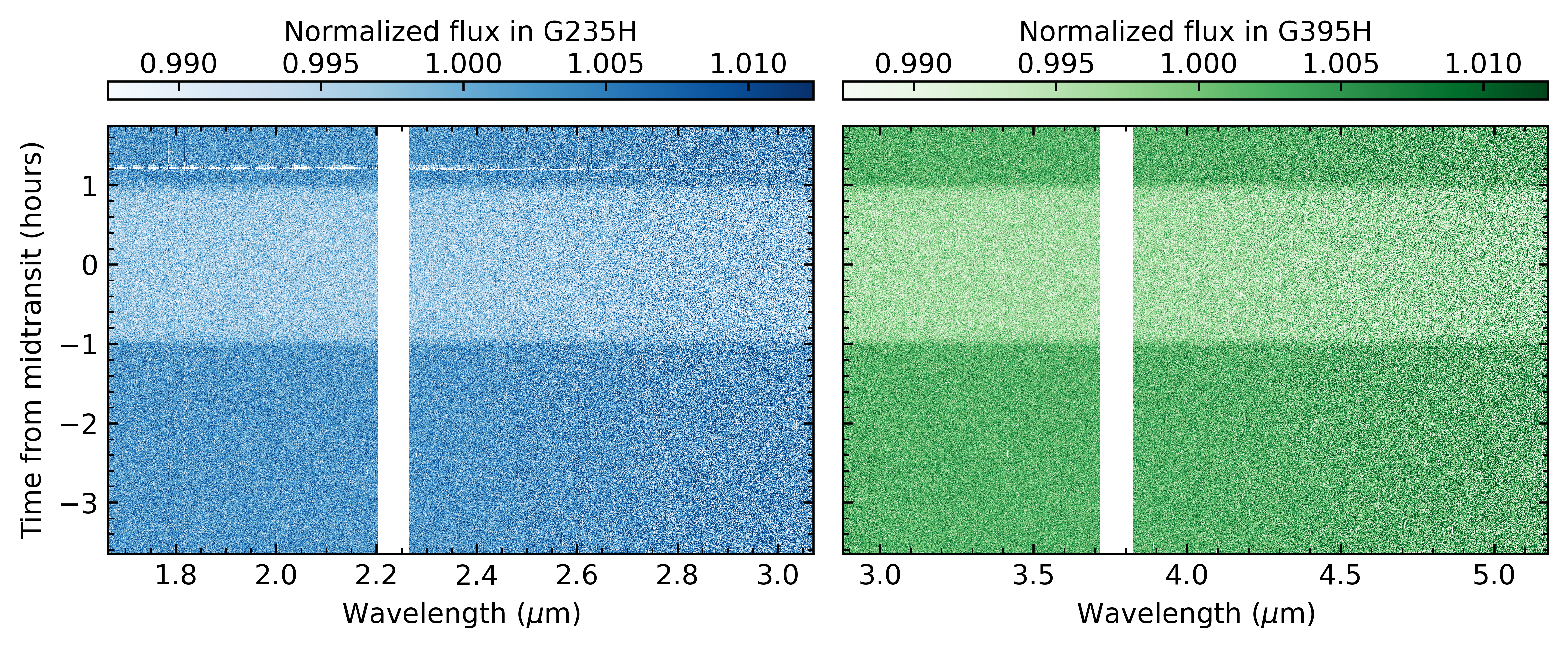
Figure 1: Raw spectroscopic light curves from the NIRSpec/G235H (left) and G395H (right) modes. Both modes show a gap that separates the data from the NRS1 and NRS2 detectors. The white horizontal stripe in the G235H data are points affected by the high-gain antenna move.

We modeled the light curves as a combination of a batman transit function (Kreidberg, 2015) and a linear polynomial in time. First, we fitted each white light curve to determine the transit midpoint ($T_{0}$), orbital inclination ($i$), and scaled semi-major axis ($a/R_{\star}$). During the white light curve fits, we kept the quadratic limb darkening coefficients free. We included a white-noise multiplier as a free parameter in the fits. We masked the integrations in the range 2134–2185 of the G235H light curves, which are affected by a high-gain antenna move (Fig. 1). Meanwhile, the G395H white light curves show a starspot crossing event, visible in both detectors (Fig. 2).

We corrected the white light curves affected by the starspot using the semi-analytical spot modeling code spotrod (Béky et al., 2014). The spot is characterized by four parameters in this model: the ratio of the spot’s radius to the star’s radius (R_spot/R_⋆), the ratio of the spot’s intensity compared to the unspotted surface of the star ($f$), and the position of the spot’s center on the star’s surface, represented by two coordinates ($\theta$, $r^{2}$). The spot-corrected white light curves are then fitted to obtain the photometric $R_{p}/R_{star}$, $T_{0}$, $i$, and $a/R_{star}$ for each of the four datasets (Table 2).

We then fitted the spectroscopic light curves at the native resolution, keeping $T_{0}$, $i$, and $a/R_{star}$ fixed to the values derived from the white light curves. We masked the integrations affected by the high-gain antenna move and the star-spot crossing event and fixed the quadratic limb darkening coefficients to those calculated by the ExoTiC-LD package (Grant & Wakeford, 2022) using 3D stellar models (Magic et al., 2015) and assuming the stellar parameters as those reported by Cadieux et al. (2024). As in the white light curve fits, we included a white-noise multiplier to ensure that the uncertainties of the results are consistent with the scatter of the residuals. We also tried fitting the spectroscopic light curves without masking the spot crossing event and found that the resulting transmission spectra were consistent.

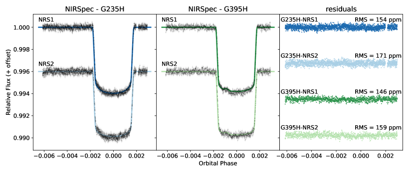
Figure 2: White light curves analysis of the two LHS 1140 b transits. The white light curve of each visit and each detector is normalized. Left panel shows the white light curves from the NRS1 and NRS2 detectors using the G235H grating. Central panel shows the same information as the left but for the G395H grating. The starspot crossing can be seen here. Right panel shows the residuals of the fit for each of the four white light curves. The relative root mean square (RMS) is also noted.

Table 2: White light curves analysis results.

Parameter	G235H – NRS1	G235H – NRS2	G395H – NRS1	G395H – NRS2
T0 [BJD]	60131.037574 $\pm$ 0.000016	60131.037605 $\pm$ 0.000018	60155.774828 $\pm$ 0.000020	60155.774826 $\pm$ 0.000022
Rp/R⋆	0.07422${}_{-0.00008}^{+0.00011}$	0.07437${}_{-0.00012}^{+0.00012}$	0.07404${}_{-0.00012}^{+0.00013}$	0.07441${}_{-0.00013}^{+0.00012}$
a/R⋆	95.6${}_{-0.7}^{+0.5}$	94.4${}_{-0.7}^{+0.7}$	95.1${}_{-0.8}^{+0.7}$	91.6${}_{-0.8}^{+0.9}$
$i$ [deg]	89.93${}_{-0.03}^{+0.03}$	89.88${}_{-0.02}^{+0.03}$	89.92${}_{-0.03}^{+0.04}$	89.81${}_{-0.02}^{+0.02}$
$u$1	0.145${}_{-0.017}^{+0.017}$	0.151${}_{-0.020}^{+0.022}$	0.091${}_{-0.022}^{+0.022}$	0.012${}_{-0.009}^{+0.016}$
$u$2	0.223${}_{-0.032}^{+0.032}$	0.152${}_{-0.039}^{+0.038}$	0.250${}_{-0.042}^{+0.040}$	0.247${}_{-0.030}^{+0.025}$

2.3 Atmospheric retrieval setup

We used the ExoTR (Exoplanetary Transmission Retrieval) algorithm to interpret the derived transmission spectrum. ExoTR is a fully Bayesian retrieval algorithm designed to interpret exoplanet transmission spectra. Its useful features include: a) the cloud layer can be modeled as an optically thick surface or as a physically motivated cloud scenario tied to a non-uniform water volume mixing ratio profile, similarly to ExoReL^ℜ (Hu, 2019; Damiano & Hu, 2020, 2022), b) the stellar heterogeneity components can be jointly fit with the planetary atmospheric parameters (Rackham et al., 2017; Pinhas et al., 2018), c) the atmospheric abundances are fit in the centered-log-ratio (CLR) space and the prior functions are designed to render a flat prior when transformed back to the log-mixing-ratio space (Damiano & Hu, 2021), and d) the possibility to fit photochemical hazes with prescribed optical constants and a free particle size. ExoTR will be described in detail in a subsequent paper (Tokadjian et al. in prep.).

In this work, we included the offset between the NRS1 and NRS2 detectors for both gratings as free parameters ($off_{n}$), given recent results using NIRSpec/G395H (e.g., Moran et al., 2023; Madhusudhan et al., 2023). We kept the NIRSpec/G235H-NRS1 dataset fixed and applied the offsets to other datasets. $off_{1}$ is the offset between NRS1 and NRS2 within the G235H grating, $off_{2}$ is the offset between G325H-NRS1 and G395H-NRS1, and $off_{3}$ is the offset between G325H-NRS1 and G395H-NRS2. Here, we adopted a simple cloud model characterized by the cloud top pressure (${\rm P}_{top}$) and kept the planetary temperature at 200 K. The atmospheric abundances are parameterized in the CLR space with H₂ or N₂ as the background gasses, and the other gases considered as free parameters in the retrieval include H₂O, CH₄, NH₃, CO₂, and CO. We jointly fit the impact of stellar heterogeneity with the planetary parameters. Three parameters were used to describe the stellar component (Pinhas et al., 2018): the star temperature ($Ts_{phot}$), the star heterogeneity temperature (either faculae or spots) ($Ts_{het}$), and the fraction of stellar surface impacted by the heterogeneity ($\delta$). The stellar spectra are adopted from the PHOENIX models (Husser et al., 2013). Table 3 lists the free parameters, the prior space used, and the range in which the parameters are probed. ExoTR uses MultiNest (Feroz et al., 2009) to sample the Bayesian evidence, estimate the parameters, and determine the posterior distribution functions. MultiNest is used through its Python implementation pymultinest (Buchner et al., 2014). For all the retrieval analyses presented here, we used 500 live points and 0.5 as the Bayesian evidence tolerance. Finally, to assess the significance of a scenario over the null hypothesis, we calculated the Bayes factor (Trotta, 2008), which is a quantitative statistical measurement to choose one model over another one.

Table 3: Model parameters and prior probability distributions used in the atmospheric retrievals. $\mathcal{U}(a,b)$ is the uniform distribution between values $a$ and $b$, $\mathcal{LU}(a,b)$ is the log-uniform (Jeffreys) distribution between values $a$ and $b$, and $\mathcal{N}(\mu,\sigma^{2})$ is the normal distribution with mean $\mu$ and variance $\sigma^{2}$. NOTE - $(^{1})$ Damiano & Hu (2021), $(^{2})$ Cadieux et al. (2024).

Parameter	Symbol	Prior
Datasets offsets [ppm]	$off_{n}$	$\mathcal{U}$(-100, 100)
Planetary radius [R⊕]	$R_{p}$	$\mathcal{U}$(0.5, 2)$\times$ R${}_{p}(^{2})$
Cloud top [Pa]	Ptop	$\mathcal{LU}$(0.0, 9.0)
VMR H2O	H2O	CLR$(-25.0,25.0)(^{1})$
VMR CH4	CH4	CLR$(-25.0,25.0)(^{1})$
VMR NH3	NH3	CLR$(-25.0,25.0)(^{1})$
VMR CO2	CO2	CLR$(-25.0,25.0)(^{1})$
VMR CO	CO	CLR$(-25.0,25.0)(^{1})$
VMR N2	N2	CLR$(-25.0,25.0)(^{1})$
Heterogeneity fraction	$\delta$	$\mathcal{U}$(0.0 - 0.5)
Heterogeneity temperature [K]	$Ts_{het}$	$\mathcal{U}$(0.5, 1.2) $\times$ $Ts_{phot}(^{2})$
Stellar temperature [K]	$Ts_{phot}$	$\mathcal{N}$(3096, 48)$(^{2})$

2.4 Self-consistent atmospheric models

We also simulated representative self-consistent atmospheric models for the potential scenarios of LHS 1140 b. We explored massive H₂-rich atmospheres with $1\times$, $10\times$, and $100\times$ solar metallicities, a small H₂-dominated atmosphere with CO₂ (i.e., a potential “hycean” scenario following Madhusudhan et al., 2021; Hu et al., 2021), as well as N₂- and CO₂-dominated atmospheres, which are plausible atmospheres overlaying a water-dominated mantle (see Sec. 4.2).

We calculated the pressure-temperature profiles for each scenario under radiative-convective equilibrium using the climate module of the ExoPlanet Atmospheric Chemistry & Radiative Interaction Simulator (EPACRIS-Climate, Scheucher et al. in prep.). The model solves the radiative fluxes using the 2-stream formulation of Heng & Marley (2018) and performs the moist adiabatic adjustment using the formulation of Graham et al. (2021). Water is treated as condensable in these models and its atmospheric abundance is self-consistently adjusted together with the moist adiabats. For simplicity, we did not include the cloud albedo feedback in these calculations, but instead applied a modest albedo of 0.3 in all models.

Based on the pressure-temperature profiles, we then simulated the effects of vertical transport and photochemistry using the chemistry module of EPACRIS. For the massive atmosphere models, we used a chemical network generated by the Reaction Mechanism Generator (Gao et al., 2016; Johnson et al., 2022) for the conditions relevant to LHS 1140 b and coupled it to the planetary-scale kinetic-transport model (Yang & Hu, 2024). For the small atmosphere models, we used the chemical network in Hu et al. (2021) together with the recent rate updates from Wogan et al. (2024). The resulting chemical abundance profiles were used together with the pressure-temperature profiles to calculate the transmission spectra. The impact of water condensation and cloud formation is self-consistently included in the transmission spectra such that the cold trap in the atmosphere controls the pressure level of the cloud and the water vapor mixing ratio above the cloud (Hu, 2019; Damiano & Hu, 2020).

3 Results

3.1 White light curves and transmission spectrum

Fig. 1 depicts the extracted and calibrated light curves at the native resolution. In the light curves obtained with the G235H grating, we observed the high-gain antenna move effect. We masked the data affected by this distortion. The high-gain antenna move happened outside the transit, and therefore masking these data does not result in any significant loss of signal.

The signal extracted from the four detectors resulted in four white light curves. Fig. 2 shows the analysis performed on each of the four white light curves as well as the residuals. The white light curves obtained with the G395H grating show the effect of a starspot crossing at the orbital phase of $\sim 0.0015$ earlier than the mid-transit point. We used spotrod (Béky et al., 2014) to fit and correct the starspot effect. First, we fit a model without the starspot using spotrod and MultiNest (Feroz et al., 2009; Espinoza et al., 2019) combined, so that we can calculate the Bayesian evidence of the model. Then, we fit a model that includes the starspot distortion. By calculating the Bayes factor, we found that the model with one starspot is preferred by the data with a significance greater than 5$\sigma$ over the light curve model without starspot. For the one starspot model, we obtained an intensity ratio of $f=0.963\pm 0.012$ and a spot-to-star radius ratio of R_spot/R${}_{\star}=0.176\pm 0.041$. The white light curve fitting results are summarized in Table 2.

The planetary and transit parameters derived from the white light curves are then fixed and used to fit the spectroscopic light curves. We did not use any binning when fitting the spectroscopic light curves, in either the time domain or the wavelength domain. After obtaining the transmission spectrum at the native resolution (R$\sim$5800), we binned the spectrum to a spectral resolution of R=65 to reveal any major molecular absorption features. The derived transmission spectrum is shown in Fig. 3.

3.2 Retrieval results

We used ExoTR described in Sec. 2.3 to interpret the transmission spectrum of LHS 1140 b. We fixed the planetary and stellar parameters to those in Table 1 and fit the atmospheric parameters in Table 3. The scenarios considered and the Bayesian evidence obtained are summarized in Table 4, and the constraints of parameters are reported in Tables 5 and 6 in Appendix A.

We considered two baseline scenarios as the null hypotheses. The first scenario assumes an H₂-only atmosphere (with Rayleigh scattering and H₂-H₂ collision-induced absorption), a generic cloud top, and the offsets between datasets. The other baseline scenario instead assumes an N₂-only atmosphere also with a generic cloud and offsets. In this way, we define the two null hypotheses with different atmospheric scale heights. We ran retrievals on the data for these two scenarios and obtained log-Bayesian evidence of ln(EV)$=$642.59 and 643.61, respectively.

On top of the baseline scenarios, we successively considered various absorbing molecules to see which ones would be favored by the data. We added H₂O to either H₂- or N₂-dominated atmosphere and H₂O and CO₂ to N₂-dominated atmosphere. We also considered the general cases where H₂, N₂, H₂O, CO₂, CH₄, NH₃, and CO are all included in the retrieval. Table 4 ranks these scenarios by the order of decreasing Bayesian evidence. We found that the models with an N₂-dominated atmosphere with H₂O and CO₂ are favored over the baseline scenarios by $>3\sigma$ (Table 4, Scenarios 1 and 2), while the inclusion of other gases does not result in the increase of evidence (Scenario 3). We also found that the Bayesian evidence does not change substantially when the stellar heterogeneity components are fit as free parameters in the retrieval (e.g., comparing Scenarios 4 and 1), and with stellar heterogeneity, the N₂-dominated atmosphere with H₂O and CO₂ is still preferred over the baseline scenarios by $\sim 3\sigma$.

The posterior distributions of Scenarios 1 and 4 are shown in Fig. 4. While both retrievals suggest solutions that range from N₂- to H₂O-dominated atmospheres, the inclusion of the stellar heterogeneity components as free parameters decrease the probability density of high mixing ratios of H₂O, suggesting that the spectral modulation seen at wavelengths $<3\mu$m may be partly due to stellar heterogeneity. In both scenarios, low mixing ratios of H₂O are possible, making an N₂-dominated atmosphere more likely (also see Table 6.)

Meanwhile, including H₂O in an H₂-dominated atmosphere results in an increase of evidence that corresponds to $\sim 2\sigma$ with respect to the baseline scenarios (Scenario 6 in Table 4). The cloud pressure required by this scenario is $\sim 10^{2.8\pm 0.5}$ Pa (Table 5). Based on the self-consistent atmospheric models, however, the water clouds should be located at a higher pressure on this planet, and an H₂-dominated atmosphere should have additional absorbing gas including CH₄ or CO₂ (see Sec. 3.3). Moreover, if we compare this scenario to an N₂-dominated atmosphere with H₂O (i.e., comparing Scenarios 6 and 2), the data still prefers the N₂-dominated atmosphere with a significance of $\sim 2.8\sigma$ (Table 4).

Lastly, we performed a joint analysis of all available datasets including the transmission spectra obtained by HST and ground-based observations (Appendix B). In that case, the spectral contribution from stellar heterogeneity is clearly required to fit the dataset across the entire wavelength range covered.

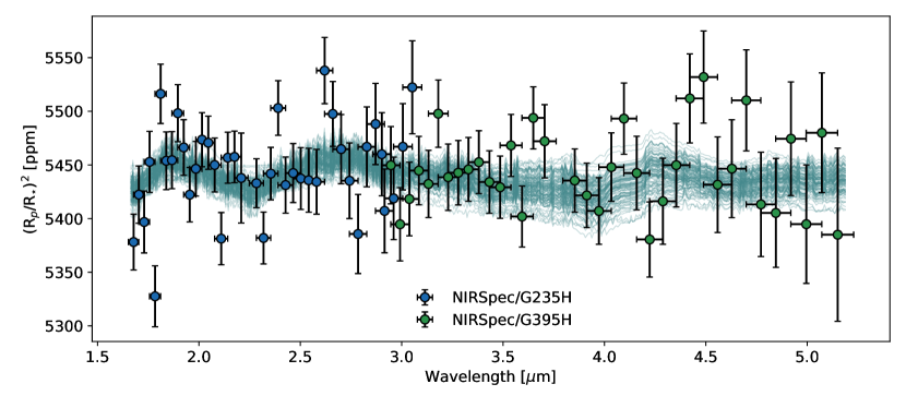
Figure 3: Transmission spectrum of LHS 1140 b. The two transit observations are color coded, i.e., blue for the G235H grating and green for the G395H grating. The models shown are randomly selected solutions from the posterior distributions of Scenario 4 (Table 4, corresponding to N₂-H₂O atmospheres with deep clouds). We have applied the best-fit offsets to the data. The offset between the two visits is $\sim 50$ ppm, while the offset between the two detectors within each of the two visits is negligible (see Figure 4 and Table 5).

Table 4: Atmospheric scenarios considered and their corresponding log-Bayesian evidence. The third and fourth columns indicate the significance level at which each scenario is favored against the baseline scenarios, obtained by calculating the Bayes factor. The offsets between the visits and the detectors have been included as free parameters for all the scenarios (3 offsets).

Free parameters	log-Bayesian Evidence, ln(EV)	$\sigma$ baseline 1	$\sigma$ baseline 2
1. N2, H2O, CO2, and cloud	647.20 $\pm$ 0.16	3.48$\sigma$	3.18$\sigma$
2. N2, H2O, and cloud	646.68 $\pm$ 0.16	3.33$\sigma$	3.02$\sigma$
3. H2, N2, H2O, CH4, NH3, CO2, CO, and cloud	646.00 $\pm$ 0.16	3.12$\sigma$	2.67$\sigma$
4. N2, H2O, CO2, cloud, and stellar heterogeneity	645.68 $\pm$ 0.16	3.03$\sigma$	2.59$\sigma$
5. H2, N2, H2O, CH4, NH3, CO2, CO, cloud, and stellar heterogeneity	645.22 $\pm$ 0.16	2.78$\sigma$	2.38$\sigma$
6. H2, H2O, and cloud	644.11 $\pm$ 0.17	2.34$\sigma$	$<$2$\sigma$
7. N2-only atmosphere with cloud (i.e., baseline 2)	643.61 $\pm$ 0.15	2.11$\sigma$	$-$
8. H2-only atmosphere with cloud (i.e., baseline 1)	642.59 $\pm$ 0.15	$-$	$-$

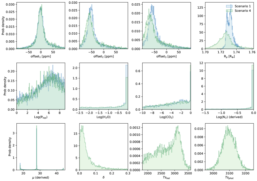
Figure 4: Comparison of the 1D posterior distribution functions of Scenarios 1 and 4 (i.e., including N₂, H₂O, CO₂, clouds and with and without the stellar heterogeneity).

3.3 Self-consistent atmospheric models

Figure 5 shows the pressure-temperature profiles of our self-consistent atmosphere models. We find that, for H₂-rich atmospheres with a wide range of metallicity, the condensation of water extends to $\sim 10^{4}$ Pa and the temperature at the cold trap would be $\sim 200$ K. Meanwhile, the atmospheric chemistry models indicate that CH₄ and NH₃ should be the most abundant carbon and nitrogen species, with appreciable amount of CO2 occurring at the high metallicity of $100\times$ solar. This behavior is similar to the findings of Hu (2021). For LHS 1140 b, due to the low temperature, the mixing ratio of H₂O is reduced by $\sim 3$ orders of magnitude above the cold trap pressure ($\sim 10^{4}$ Pa). As a result, the transmission spectra of a massive H₂-rich atmosphere on LHS 1140 b, regardless of metallicity, would at least show strong spectral features of CH₄, which is clearly ruled out by the transmission spectrum presented here (Fig. 6).

If the planet has a small H₂-dominated atmosphere on top of an H₂O-dominated mantle, the dominant form of carbon should be CO₂ (Hu et al., 2021; Wogan et al., 2024) and NH₃ should be either removed by photolysis or dissolved in the oceans (Yu et al., 2021; Hu et al., 2021). The transmission spectrum of this scenario would have strong CO₂ features, which is also clearly ruled out by the transmission spectrum presented here (Fig. 6).

Lastly, we considered an N₂-dominated atmosphere (with 10% CO₂) and a CO₂-dominated atmosphere (with 10% N₂) for the planet. With a surface pressure of 2.2 bar, we found that the surface temperatures of these two scenarios would be $\sim 310$ and $\sim 340$ K, consistent with liquid water. We caution that these temperatures are substantially higher than the surface temperatures predicted by 3D climate models (Cadieux et al., 2024). One possible reason for the discrepancy may be that the 3D models have a proper account of the ice-albedo effect. With the high mean molecular weight to subdue the transmission features, these models provide a reasonable fit to the spectrum (Fig. 6). Notably, the models do not show significant absorption of water vapor as it has condensed out from the part of the atmosphere probed by transmission spectra, and the only spectral features that could be observed are CO₂ absorption. This is consistent with the models presented in Cadieux et al. (2024). At $\sim 4.2\ \mu$m, our model suggests a $\sim$20-ppm CO₂ absorption feature.

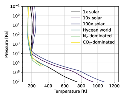
Figure 5: Modeled pressure-temperature profiles for LHS 1140 b, considering massive H₂-rich atmospheres with $1\times$, $10\times$, and $100\times$ solar metallicity abundances, and small (2.2-bar) H₂-, N₂-, and CO₂-dominated atmospheres. The small H₂-dominated atmosphere has 1% CO₂, corresponding to the proposed “hycean world” scenario for temperate sub-Neptunes (Madhusudhan et al., 2021; Hu et al., 2021). The temperature profiles indicate a cold trap at the pressure of $\sim 10^{4}$ Pa for the H₂-rich atmospheres and $\sim 10^{4.5}$ Pa for N₂- and CO₂-dominated atmospheres. The resulting transmission spectra of these models are shown in Fig. 6.

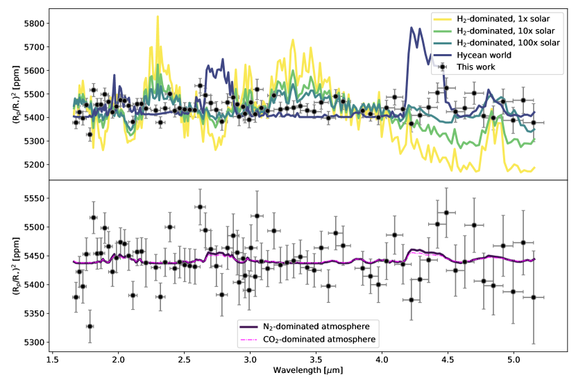
Figure 6: Self-consistent atmospheric models of LHS 1140 b compared to the JWST data. Top panel shows the massive H₂-rich atmosphere models with varied metallicities as well as the small H₂-dominated atmosphere with CO₂ model (“hycean world”). $\chi^{2}=$1405, 506, and 289 for the $1\times$, $10\times$, and $100\times$ solar metallicity models, respectively, and $\chi^{2}=$473 for the hycean model. These models are ruled out by the data with a p-value $<0.00001$. Bottom panel shows the N₂- and CO₂-dominated atmosphere models. $\chi^{2}=$118 for both models.

4 Discussion

4.1 Excluding the H₂-rich atmosphere scenarios

The observations presented here were originally designed to detect an H₂-rich atmosphere with the possible presence of water vapor and other gases (e.g., methane and carbon dioxide). However, the transmission spectrum obtained makes an H₂-dominated atmosphere highly unlikely. Our atmospheric models show that, regardless of the atmospheric metallicity or size, an H₂-rich atmosphere on LHS 1140 b should result in detectable spectral features of either CH₄ or CO₂ (Fig. 6). Because of the low temperature of the planet, H₂O is condensed out at a higher pressure than the region typically probed by transmission spectra. This eliminates the potentially confounding scenario of a highly metal-rich H₂ atmosphere (Benneke et al., 2024), because such a scenario would still result in detectable spectral features of CH₄ and CO₂.

From the point of view of spectral retrievals, Table 4 shows that the data favor a high mean molecular weight atmosphere with the presence of water vapor. The data could be marginally explained by an H₂-dominated atmosphere with high clouds ($\sim$10^2.8 Pa) and low water vapor mixing ratio ($\sim$10^-4) (Scenario 6, see Tables 5 and 6 for detailed constraints). However, our atmospheric models show that the water clouds should extend to $\sim 10^{4}$ Pa but not lower pressures. We have also checked for the condensation of NH₃ and the formation of NH₄SH clouds in the self-consistent atmospheric models shown in Figs. 5 and 6 using the method of Hu (2021), and found that NH₃ should not condense, and the NH₄SH clouds, if forming, should only occur within a pressure scale height of the cold trap, having a minimal impact to the transmission spectra. Besides, such an H₂-dominated atmosphere should also have an appreciable abundance of CH₄ (if massive) or CO₂ (if small), and they would result in spectral features detectable in $3-5\ \mu$m. Therefore H₂-dominated atmosphere with high clouds scenario is unlikely to apply for LHS 1140 b.

One might ask if a high-altitude haze layer might create the flat spectrum. Given the low temperature of the planet, the plausible photochemical haze in a H₂-rich atmosphere includes sulfur haze from H₂S and hydrocarbon haze from CH₄. Atmospheric chemistry calculations indicated that the sulfur haze, if any, should be located at a similar pressure level as the water cloud and thus not impact the transmission spectrum (Hu, 2021). Hydrocarbon haze, on the other hand, can be produced from the photolysis of CH₄ in the upper atmosphere. However, this mechanism cannot explain the transmission spectrum of LHS 1140 b because, first, we do not detect any signals of CH₄ and second, such a haze layer would result in a slope in the transmission spectrum in the spectral range probed by JWST observations (Robinson et al., 2014; Kawashima et al., 2019; Gao & Zhang, 2020), which is not observed here. Lastly, we would like to point out that any massive H₂-rich atmosphere on LHS 1140 b should have abundant CH₄, which would cause a moderate temperature inversion in the middle atmosphere due to shortwave absorption (Fig. 5). Such a stratified atmosphere would also facilitate the fall off of any large photochemical haze particles, giving rise to a spectral slope if any detectable photochemical haze is present at all.

4.2 Possible habitable water world

Without a massive H₂-rich atmosphere, the most plausible explanation for LHS 1140 b’s low density is a water-rich envelope. Given the low irradiation and $\sim 10\%$ water by mass (Cadieux et al., 2024), LHS 1140 b is likely to have a high-pressure (HP) ice mantle (e.g., Sotin et al., 2007; Fu et al., 2009; Zeng & Sasselov, 2014), which itself may be partly or fully mixed with the rocky mantle underneath (e.g., Vazan et al., 2022; Kovačević et al., 2022). Meanwhile, we could expect that C- and N-bearing ices were accreted together with H₂O ice when the planet formed (Öberg et al., 2011; Schwarz & Bergin, 2014). With the accretional heat, those C- and N-bearing molecules would be thermally equilibrated with a reservoir of H₂O, resulting in predominantly CO₂ and N₂. Thus, the planet could reasonably have an N₂- or CO₂-dominated atmosphere.

The partitioning of C, N, and O molecules between the ice/rock mantle and atmosphere controls the atmospheric size and composition (Levi et al., 2017; Marounina & Rogers, 2020). For example, depending on the planet’s thermal evolution history, CO₂ can be stored in the interior as clathrate hydrates, liquids, and various types of ices (Figure 7), which could give rise to a moderate-size atmosphere and a surface temperature conducive to liquid water. Alternatively, if the entirety of the planet’s carbon and nitrogen presents as gas-phase N₂ and CO₂, this could result in a massive atmosphere and supercritical water layer (Levi et al., 2017; Marounina & Rogers, 2020).

It is therefore crucial to maintain the size of the N₂-CO₂ atmosphere for a habitable state to emerge. Silicate weathering as the key atmosphere/climate stabilizing mechanism for rocky planets is likely not applicable for LHS 1140 b, due to a lack of exposed landmasses and decoupling between the deep ocean and the atmosphere. Alternatively, the entrapment and depletion of CO₂ as clathrate-rich sea ice could help sustain a stable CO₂ atmospheric pressure suitable for liquid water (Ramirez & Levi, 2018). This mechanism works because CO₂ clathrate hydrate is denser than water and is thermodynamically stable in the deep CO₂-saturated ocean. And therefore, the formation and sinking of CO₂ clathrates in the cooler part of the planet (e.g., the night side) could maintain a CO₂ atmosphere to $<\sim 10$ bar. The workings of this mechanism on LHS 1140 b, which can be assumed to be tidally locked (Leconte et al., 2015), requires further studies.

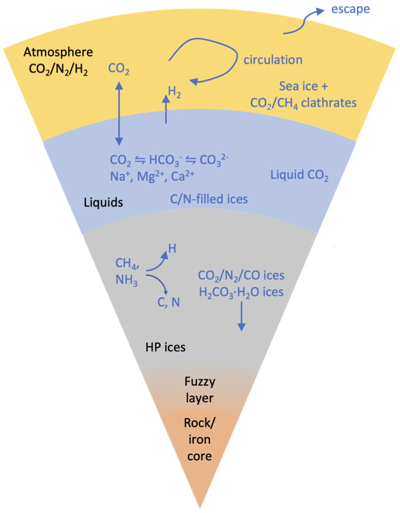
Figure 7: Potential processes that partition C and N species between the atmosphere, the ocean, and the HP ices in a cold water world like LHS 1140 b. Summarized based on Levi et al. (2017); Ramirez & Levi (2018); Levi & Cohen (2019); Marounina & Rogers (2020); Vazan et al. (2022); Kovačević et al. (2022).

4.3 Prospect for future observations

The N₂-CO₂ atmosphere scenarios result in small but potentially detectable spectral features of CO₂ absorption (Fig. 6). Using PandExo (Batalha et al., 2017), we find that an additional 9 transits with NIRSpec/G395M would be required to achieve a precision of 20 ppm at $\sim 4.2\ \mu$m to detect the CO₂ absorption feature. This estimate is in line with those presented in Cadieux et al. (2024).

Considering the rarity of LHS 1140 b transit events, a campaign of 9 additional transits would require a few years to complete. In addition, obtaining transit measurements using NIRISS/SOSS could help to disentangle the stellar heterogeneity component from the planetary atmospheric signature, benefiting from the continuous coverage from 0.6 to 2.8 $\mu$m. However, we do not yet understand how the stellar activity would change from visit to visit and this may prevent combining multiple NIRISS observations or using NIRISS observations to constrain NIRSpec/G395M observations directly. We note that two transit observations of LHS 1140 b have been taken using NIRISS/SOSS in December 2023 (Program ID: 6543, PI: Cadieux, C.). Those observations could provide updated constraints on the stellar heterogeneity component and refinements to the transmission spectrum of LHS 1140 b at wavelengths $<3\ \mu$m.

5 Conclusions

In this paper, we present the data analysis of the two primary transit observations of LHS 1140 b performed by JWST using the NIRSpec instrument. The observations cover a spectral range between 1.7 and 5.2 $\mu$m. The transmission spectrum resulting from the JWST data shows a constant transit depth as a function of wavelength, indicating no apparent absorption features. Because an H₂-rich atmosphere on this planet would show strong transmission spectral features from CH₄ or CO₂, the spectrum presented here rules out an H₂-rich atmosphere on LHS 1140 b.

We used a Bayesian retrieval framework, ExoTR, to interpret the transmission spectrum together with the stellar heterogeneity and found that the data favors an N₂-dominated atmosphere with H₂O and CO₂ over an H₂-dominated atmosphere with high clouds or an N₂-dominated atmosphere without any molecular absorption by $3\sigma$ confidence. The H₂-dominated atmosphere with high clouds or photochemical haze is unlikely because the expected water cloud is deep in the atmosphere (at $>\sim 10^{4}$ Pa) and the spectrum does not show any signals of CH₄ which is the feedstock to form photochemical haze.

The observation and analysis presented here effectively leave a water-dominated layer as the only plausible explanation for the low density of the planet. Also, the water world cannot have a small H₂-dominated atmosphere, i.e., not a “hycean world.” Rather, based on planetary evolution considerations, we suggest that an N₂- or CO₂-dominated atmosphere is likely and consistent with the transmission spectrum presented here. Our climate model indicates that a moderate-size ($\sim 2$ bar) N₂- or CO₂-dominated atmosphere could maintain a global mean surface temperature above the freezing point of water. If the planet evolves to or has the climate-stabilizing mechanism to maintain such a moderate-size N₂- or CO₂-dominated atmosphere, the planet may be a habitable water world.

LHS 1140 b is thus a unique planet that provides the rare opportunity to observe and characterize a temperate, potentially habitable water worlds. We estimated that 9 additional transits are required to detect CO₂ in the high mean molecular weight atmosphere on this planet, and this could be completed in $\sim 3$ JWST cycles. With the existence of an atmosphere on TRAPPIST-1 planets called into question (Dong et al., 2018; Greene et al., 2023; Zieba et al., 2023), LHS 1140 b may well present the best current opportunity to detect and characterize a habitable world in our interstellar neighborhood.

Data availability

All the JWST data used in this paper can be found in MAST: http://dx.doi.org/10.17909/r627-v590 (catalog 10.17909/r627-v590). Raw data will be publicly available after the proprietary period (i.e., August 2024).

Software

ExoTR, Numpy (Oliphant, 2015), Scipy (Virtanen et al., 2020), Astropy (Price-Whelan et al., 2018), scikit-bio (scikit-bio development team, 2020), Matplotlib (Hunter, 2007), MultiNest (Feroz et al., 2009; Buchner et al., 2014), mpi4py (Dalcin & Fang, 2021), spotrod (Béky et al., 2014), Eureka! (Bell et al., 2022), ExoTiC-LD (Grant & Wakeford, 2022), batman (Kreidberg, 2015), PandExo (Batalha et al., 2017).

Appendix A Scenarios retrieval results

Tables 5 and 6 contain the results of the retrieval analyses performed on the scenarios listed in Table 4.

Table 5: Retrieval results for the scenarios presented in Table 4. The offsets are defined relative to the NIRSpec/G325H-NRS1 dataset. Therefore, $off_{1}$ is the offset between NRS1 and NRS2 within the G235H grating, $off_{2}$ is the offset between the G325H-NRS1 and G395H-NRS1, and $off_{3}$ is the offset between the G325H-NRS1 and G395H-NRS2.

Scenario	$off_{1}$	$off_{2}$	$off_{3}$	Rp [R⊕]	Log(Ptop)	$\delta$	Thet	Tphot
1.	-0.73${}^{+8.99}_{-8.78}$	-52.89${}^{+8.89}_{-9.02}$	-59.20${}^{+10.79}_{-10.53}$	1.730$\pm$0.003	6.48${}^{+1.68}_{-1.94}$	$-$	$-$	$-$
2.	0.23${}^{+7.78}_{-9.07}$	-51.52${}^{+9.05}_{-9.57}$	-66.35${}^{+10.51}_{-10.98}$	1.732$\pm$0.002	6.49${}^{+1.66}_{-1.85}$	$-$	$-$	$-$
3.	2.42${}^{+9.37}_{-7.95}$	-51.57${}^{+9.22}_{-8.81}$	-60.85${}^{+11.03}_{-9.95}$	1.728$\pm$0.002	5.93${}^{+1.93}_{-1.91}$	$-$	$-$	$-$
4.	-2.10${}^{+8.32}_{-8.34}$	-59.88${}^{+10.52}_{-11.58}$	-69.01${}^{+12.98}_{-14.10}$	1.725$\pm$0.006	6.37${}^{+1.69}_{-1.97}$	0.02${}^{+0.03}_{-0.01}$	2641${}^{+410}_{-517}$	3098$\pm$45
5.	1.39${}^{+8.23}_{-8.76}$	-57.26${}^{+10.46}_{-10.73}$	-68.30${}^{+13.33}_{-13.98}$	1.724$\pm$0.004	5.91${}^{+1.99}_{-2.15}$	0.03${}^{+0.05}_{-0.02}$	2941${}^{+168}_{-325}$	3097$\pm$41
6.	4.25${}^{+9.09}_{-9.23}$	-57.14${}^{+9.72}_{-8.08}$	-64.45${}^{+8.89}_{-9.82}$	1.657$\pm$0.007	2.82${}^{+0.45}_{-0.58}$	$-$	$-$	$-$
7.	-5.09${}^{+9.07}_{-8.82}$	-54.74${}^{+9.87}_{-9.82}$	-60.72${}^{+10.71}_{-11.13}$	1.732$\pm$0.003	3.59${}^{+2.99}_{-2.46}$	$-$	$-$	$-$
8.	-4.16${}^{+8.84}_{-8.97}$	-53.81${}^{+8.91}_{-9.96}$	-60.03${}^{+10.53}_{-10.76}$	1.641$\pm$0.013	1.59${}^{+1.04}_{-1.06}$	$-$	$-$	$-$

Table 6: Retrieval results on the atmospheric abundances for the scenarios presented in Table 4.

Scenario	Log(H2O)	Log(CH4)	Log(NH3)	Log(CO)	Log(CO2)	Log(N2)	Log(H2)	$\mu$ (derived)
1.	-0.34${}^{+0.33}_{-3.38}$	$-$	$-$	$-$	-2.32${}^{+1.51}_{-3.09}$	-0.84${}^{+0.84}_{-3.25}$	$-$	25.45${}^{+2.65}_{-7.19}$
2.	-2.19${}^{+1.61}_{-2.13}$	$-$	$-$	$-$	$-$	-0.01${}^{+0.01}_{-0.13}$	$-$	27.95${}^{+0.06}_{-2.55}$
3.	-0.05${}^{+0.05}_{-1.42}$	-6.83${}^{+1.78}_{-2.03}$	-4.58${}^{+3.04}_{-3.26}$	-3.18${}^{+2.58}_{-3.22}$	-4.32${}^{+2.98}_{-3.77}$	-3.91${}^{+2.78}_{-3.33}$	-5.16${}^{+3.18}_{-3.91}$	18.50${}^{+8.97}_{-0.52}$
4.	-1.31${}^{+1.29}_{-3.03}$	$-$	$-$	$-$	-2.71${}^{+2.02}_{-3.59}$	-0.15${}^{+0.15}_{-2.77}$	$-$	27.98${}^{+0.79}_{-9.17}$
5.	-0.27${}^{+0.26}_{-2.21}$	-6.53${}^{+1.97}_{-2.26}$	-4.55${}^{+3.12}_{3.09}$	-3.00${}^{+2.54}_{-3.23}$	-3.43${}^{+2.81}_{-4.22}$	-3.19${}^{+2.64}_{-3.60}$	-5.14${}^{+3.45}_{-4.67}$	20.42${}^{+7.73}_{-2.43}$
6.	-4.20${}^{+0.93}_{-0.59}$	$-$	$-$	$-$	$-$	$-$	-0.01${}^{+0.01}_{-0.01}$	2.02$\pm$0.01
7.	$-$	$-$	$-$	$-$	$-$	0.00	$-$	28.00
8.	$-$	$-$	$-$	$-$	$-$	$-$	0.00	2.02

Appendix B Joint fit of groudbased, HST, and JWST data

Given its intriguing physical parameters, LHS 1140 b has been the object of several observation campaigns to unveil the atmospheric composition and assess the nature of the planet. HST initially observed the planet in January and December of 2017 (program ID: 14888, PI: Dittmann, J.) for an initial reconnaissance of the planet’s transmission spectrum between $\sim$1.1 and $\sim$1.6 $\mu$m. The resulting 1D transmission spectrum suggests strong spectral modulations that may be attributed to H₂O. If the spectral modulation truly has a planetary origin, the planet should have an H₂-dominated atmosphere (Edwards et al., 2020). Another campaign was conducted between 2017 and 2018 to observe the planet in transmission spectroscopy in the visible band with the Magellan telescope at Las Campanas Observatory. The obtained spectrum revealed a strong linear trend due to the stellar heterogeneity (Diamond-Lowe et al., 2020).

The HST and JWST datasets do not appear to be consistent with each other. Fig. 8 compares the solution of the spectral retrieval performed on the HST observation with the JWST data, and it shows that the data and the model are incompatible. In particular, the lack of the H₂-H₂ CIA spectral feature is clear between 2 and 3 $\mu$m.

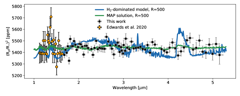
Figure 8: The transmission spectrum obtained in this work compared with the HST data adopted from Edwards et al. (2020). The green model, i.e., maximum a posteriori (MAP) solution, is the same as the one depicted in Fig. 3 extended to the HST data wavelength. The blue model is the best fit model for the HST data (an H₂-dominated atmosphere with water vapour absorption) with a CH₄ and CO₂ 10^-6 VMR injected extended to the wavelength range covered by the JWST data. The JWST dataset is incompatible with the blue model.

Under the assumption that the stellar heterogeity signal remains constant between epoches (which is likely not true), we performed a joint fit of all the datasets aforementioned together with the the JWST data presented in this work (Figs. 9 and 10) to fit the stellar heterogeity component and assess whether or not a high mean molecular weight atmosphere is still a statistically preferred by the data. The visible-wavelength dataset helps primarily to fit the stellar heterogeneity contribution to the transmission spectrum. The stellar heterogeneity also contributes at longer wavelengths, but not significantly beyond 3 $\mu$m. According to the resulting posterior distribution functions in Fig. 10, the combined data do not favor an H₂-dominated atmosphere, but rather an H₂O-dominated atmosphere, potentially with some amounts of H₂. This is largely consistent with the results presented in Sec. 3, where a high mean molecular weight atmosphere is preferred. The non negligible amount of H₂ mainly comes form the fitting of the HST data. In that dataset, the spectral feature around 1.3$\mu$m is significant. The difference in (R_p/R_⋆)² between the peak at 1.38 $\mu$m and the baseline is approximately 200 ppm. The pressure scale height of an H₂-dominated atmosphere around LHS 1140 b is $\sim$35 km, corresponding to 38 ppm. Therefore, the potential spectral variation would correspond to approximately 5 pressure scale heights in an H₂-dominated atmosphere. However, the JWST data, as explained in Sections 3 and 4, do not show such large spectral features. It is entirely possible that the HST dataset suffers from a particularly intense episode of stellar heterogeneity.

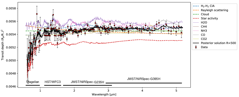
Figure 9: Available datasets for LHS 1140 b. The maximum a posteriori solution from the Bayesian retrieval process is shown in black. The individual contribution from the spectral components is also shown. The data is plotted by taking into consideration the offsets value calculated by the Bayesian analysis. The offsets value are reported in the posterior distribution functions in Fig. 10. HST data are adopted from (Edwards et al., 2020) and the Magellan data are adopted from (Diamond-Lowe et al., 2020).

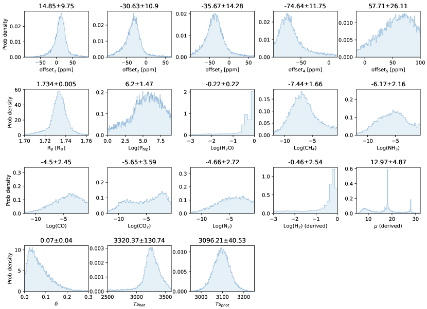
Figure 10: Posterior distribution functions of the Bayesian analysis of all the LHS 1140 b datasets combined. The posterior distribution functions suggest an H₂O-rich atmosphere with a non-negligible presence of hydrogen. The offsets are defined as follows: $offset_{1}$ is related with the G235H - NRS2, and $offset_{2}$ and $offset_{3}$ are instead relative to the G395H - NRS1 and NRS2 respectively. $offset_{4}$ is between the HST data (Edwards et al., 2020) and G325H-NRS1 dataset and $offset_{5}$ is between the Magellan dataset (Diamond-Lowe et al., 2020) and the G325H-NRS1 data. The numeric values above each panel indicate the median and $1\sigma$ uncertainty of the distribution.

References

- Ahrer et al. (2023) Ahrer, E.-M., Stevenson, K. B., Mansfield, M., et al. 2023, Nature, 614, 653, doi: 10.1038/s41586-022-05590-4
- Alderson et al. (2023) Alderson, L., Wakeford, H. R., Alam, M. K., et al. 2023, Nature, 614, 664, doi: 10.1038/s41586-022-05591-3
- Batalha et al. (2017) Batalha, N. E., Mandell, A., Pontoppidan, K., et al. 2017, PASP, 129, 064501, doi: 10.1088/1538-3873/aa65b0
- Béky et al. (2014) Béky, B., Kipping, D. M., & Holman, M. J. 2014, MNRAS, 442, 3686, doi: 10.1093/mnras/stu1061
- Bell et al. (2022) Bell, T. J., Ahrer, E.-M., Brande, J., et al. 2022, Journal of Open Source Software, 7, 4503, doi: 10.21105/joss.04503
- Benneke et al. (2024) Benneke, B., Roy, P.-A., Coulombe, L.-P., et al. 2024, arXiv preprint arXiv:2403.03325
- Buchner et al. (2014) Buchner, J., Georgakakis, A., Nandra, K., et al. 2014, A&A, 564, A125, doi: 10.1051/0004-6361/201322971
- Cadieux et al. (2024) Cadieux, C., Plotnykov, M., Doyon, R., et al. 2024, The Astrophysical Journal Letters, 960, L3, doi: 10.3847/2041-8213/ad1691
- Chakrabarty & Mulders (2023) Chakrabarty, A., & Mulders, G. D. 2023, arXiv preprint arXiv:2310.03593
- Dalcin & Fang (2021) Dalcin, L., & Fang, Y.-L. L. 2021, Computing in Science & Engineering, 23, 47, doi: 10.1109/MCSE.2021.3083216
- Damiano & Hu (2020) Damiano, M., & Hu, R. 2020, AJ, 159, 175, doi: 10.3847/1538-3881/ab79a5
- Damiano & Hu (2021) —. 2021, AJ, 162, 200, doi: 10.3847/1538-3881/ac224d
- Damiano & Hu (2022) —. 2022, AJ, 163, 299, doi: 10.3847/1538-3881/ac6b97
- Diamond-Lowe et al. (2020) Diamond-Lowe, H., Berta-Thompson, Z., Charbonneau, D., Dittmann, J., & Kempton, E. M.-R. 2020, The Astronomical Journal, 160, 27, doi: 10.3847/1538-3881/ab935f
- Dittmann et al. (2017) Dittmann, J. A., Irwin, J. M., Charbonneau, D., et al. 2017, Nature, 544, 333, doi: 10.1038/nature22055
- Dong et al. (2018) Dong, C., Jin, M., Lingam, M., et al. 2018, Proceedings of the National Academy of Sciences, 115, 260
- Edwards et al. (2020) Edwards, B., Changeat, Q., Mori, M., et al. 2020, The Astronomical Journal, 161, 44, doi: 10.3847/1538-3881/abc6a5
- Espinoza et al. (2019) Espinoza, N., Rackham, B. V., Jordán, A., et al. 2019, MNRAS, 482, 2065, doi: 10.1093/mnras/sty2691
- Feroz et al. (2009) Feroz, F., Hobson, M. P., & Bridges, M. 2009, Monthly Notices of the Royal Astronomical Society, 398, 1601, doi: 10.1111/j.1365-2966.2009.14548.x
- Fu et al. (2009) Fu, R., O’Connell, R. J., & Sasselov, D. D. 2009, The Astrophysical Journal, 708, 1326
- Gao et al. (2016) Gao, C. W., Allen, J. W., Green, W. H., & West, R. H. 2016, Computer Physics Communications, 203, 212, doi: https://doi.org/10.1016/j.cpc.2016.02.013
- Gao & Zhang (2020) Gao, P., & Zhang, X. 2020, The Astrophysical Journal, 890, 93
- Gillon et al. (2017) Gillon, M., Triaud, A. H., Demory, B.-O., et al. 2017, Nature, 542, 456
- Goldblatt (2015) Goldblatt, C. 2015, Astrobiology, 15, 362
- Graham et al. (2021) Graham, R. J., Lichtenberg, T., Boukrouche, R., & Pierrehumbert, R. T. 2021, \psj, 2, 207, doi: 10.3847/PSJ/ac214c
- Grant & Wakeford (2022) Grant, D., & Wakeford, H. R. 2022, Exo-TiC/ExoTiC-LD: ExoTiC-LD v3.0.0, v3.0.0, Zenodo, doi: 10.5281/zenodo.7437681. https://doi.org/10.5281/zenodo.7437681
- Greene et al. (2023) Greene, T. P., Bell, T. J., Ducrot, E., et al. 2023, Nature, 618, 39
- Heng & Marley (2018) Heng, K., & Marley, M. S. 2018, Radiative Transfer for Exoplanet Atmospheres, ed. H. J. Deeg & J. A. Belmonte (Cham: Springer International Publishing), 2137–2152. https://doi.org/10.1007/978-3-319-55333-7_102
- Hu (2019) Hu, R. 2019, The Astrophysical Journal, 887, 166
- Hu (2021) —. 2021, The Astrophysical Journal, 921, 27
- Hu et al. (2021) Hu, R., Damiano, M., Scheucher, M., et al. 2021, The Astrophysical Journal Letters, 921, L8
- Hunter (2007) Hunter, J. D. 2007, Computing in Science & Engineering, 9, 90, doi: 10.1109/MCSE.2007.55
- Husser et al. (2013) Husser, T. O., Wende-von Berg, S., Dreizler, S., et al. 2013, A&A, 553, A6, doi: 10.1051/0004-6361/201219058
- Innes et al. (2023) Innes, H., Tsai, S.-M., & Pierrehumbert, R. T. 2023, arXiv preprint arXiv:2304.02698
- Izidoro et al. (2022) Izidoro, A., Schlichting, H. E., Isella, A., et al. 2022, The Astrophysical Journal Letters, 939, L19
- Johnson et al. (2022) Johnson, M. S., Dong, X., Grinberg Dana, A., et al. 2022, Journal of Chemical Information and Modeling, 62, 4906, doi: 10.1021/acs.jcim.2c00965
- JWST Transiting Exoplanet Community Early Release Science Team et al. (2023) JWST Transiting Exoplanet Community Early Release Science Team, Ahrer, E.-M., Alderson, L., et al. 2023, Nature, 614, 649, doi: 10.1038/s41586-022-05269-w
- Kawashima et al. (2019) Kawashima, Y., Hu, R., & Ikoma, M. 2019, The Astrophysical Journal Letters, 876, L5
- Koll & Cronin (2019) Koll, D. D., & Cronin, T. W. 2019, The Astrophysical Journal, 881, 120
- Kopparapu et al. (2013) Kopparapu, R. K., Ramirez, R., Kasting, J. F., et al. 2013, ApJ, 770, 82, doi: 10.1088/0004-637X/770/1/82
- Kovačević et al. (2022) Kovačević, T., González-Cataldo, F., Stewart, S. T., & Militzer, B. 2022, Scientific reports, 12, 13055
- Kreidberg (2015) Kreidberg, L. 2015, PASP, 127, 1161, doi: 10.1086/683602
- Kunimoto et al. (2022) Kunimoto, M., Winn, J., Ricker, G. R., & Vanderspek, R. K. 2022, AJ, 163, 290, doi: 10.3847/1538-3881/ac68e3
- Leconte et al. (2015) Leconte, J., Wu, H., Menou, K., & Murray, N. 2015, Science, 347, 632
- Leconte et al. (2024) Leconte, J., Spiga, A., Clément, N., et al. 2024, arXiv preprint arXiv:2401.06608
- Levi & Cohen (2019) Levi, A., & Cohen, R. E. 2019, The Astrophysical Journal, 882, 71
- Levi et al. (2017) Levi, A., Sasselov, D., & Podolak, M. 2017, The Astrophysical Journal, 838, 24
- Lillo-Box et al. (2020) Lillo-Box, J., Figueira, P., Leleu, A., et al. 2020, Astronomy & Astrophysics, 642, A121, doi: 10.1051/0004-6361/202038922
- Lim et al. (2023) Lim, O., Benneke, B., Doyon, R., et al. 2023, The Astrophysical Journal Letters, 955, L22
- Luque & Pallé (2022) Luque, R., & Pallé, E. 2022, Science, 377, 1211
- Lustig-Yaeger et al. (2023) Lustig-Yaeger, J., Fu, G., May, E. M., et al. 2023, Nature Astronomy, 7, 1317, doi: 10.1038/s41550-023-02064-z
- Madhusudhan et al. (2021) Madhusudhan, N., Piette, A. A., & Constantinou, S. 2021, The Astrophysical Journal, 918, 1
- Madhusudhan et al. (2023) Madhusudhan, N., Sarkar, S., Constantinou, S., et al. 2023, ApJ, 956, L13, doi: 10.3847/2041-8213/acf577
- Magic et al. (2015) Magic, Z., Chiavassa, A., Collet, R., & Asplund, M. 2015, Astronomy & Astrophysics, 573, A90
- Marounina & Rogers (2020) Marounina, N., & Rogers, L. A. 2020, The Astrophysical Journal, 890, 107
- May et al. (2023) May, E., MacDonald, R. J., Bennett, K. A., et al. 2023, The Astrophysical Journal Letters, 959, L9
- Ment et al. (2019) Ment, K., Dittmann, J. A., Astudillo-Defru, N., et al. 2019, AJ, 157, 32, doi: 10.3847/1538-3881/aaf1b1
- Moran et al. (2023) Moran, S. E., Stevenson, K. B., Sing, D. K., et al. 2023, The Astrophysical Journal Letters, 948, L11
- Öberg et al. (2011) Öberg, K. I., Murray-Clay, R., & Bergin, E. A. 2011, The Astrophysical Journal Letters, 743, L16
- Oliphant (2015) Oliphant, T. 2015, Guide to NumPy (Continuum Press). https://books.google.com/books?id=g58ljgEACAAJ
- Pinhas et al. (2018) Pinhas, A., Rackham, B. V., Madhusudhan, N., & Apai, D. 2018, MNRAS, 480, 5314, doi: 10.1093/mnras/sty2209
- Price-Whelan et al. (2018) Price-Whelan, A. M., Sipőcz, B. M., Günther, H. M., et al. 2018, The Astronomical Journal, 156, 123, doi: 10.3847/1538-3881/aabc4f
- Rackham et al. (2017) Rackham, B., Espinoza, N., Apai, D., et al. 2017, ApJ, 834, 151, doi: 10.3847/1538-4357/aa4f6c
- Rackham et al. (2018) Rackham, B. V., Apai, D., & Giampapa, M. S. 2018, The Astrophysical Journal, 853, 122
- Ramirez & Levi (2018) Ramirez, R. M., & Levi, A. 2018, Monthly Notices of the Royal Astronomical Society, 477, 4627
- Robinson et al. (2014) Robinson, T. D., Maltagliati, L., Marley, M. S., & Fortney, J. J. 2014, Proceedings of the National Academy of Sciences, 111, 9042
- Rogers et al. (2023) Rogers, J. G., Schlichting, H. E., & Owen, J. E. 2023, The Astrophysical Journal Letters, 947, L19
- Rogers (2015) Rogers, L. A. 2015, The Astrophysical Journal, 801, 41
- Schwarz & Bergin (2014) Schwarz, K. R., & Bergin, E. A. 2014, The Astrophysical Journal, 797, 113
- scikit-bio development team (2020) scikit-bio development team, T. 2020, scikit-bio: A Bioinformatics Library for Data Scientists, Students, and Developers, 0.5.5. http://scikit-bio.org
- Seager & Deming (2010) Seager, S., & Deming, D. 2010, Annual Review of Astronomy and Astrophysics, 48, 631
- Sebastian et al. (2021) Sebastian, D., Gillon, M., Ducrot, E., et al. 2021, A&A, 645, A100, doi: 10.1051/0004-6361/202038827
- Sotin et al. (2007) Sotin, C., Grasset, O., & Mocquet, A. 2007, Icarus, 191, 337
- Trotta (2008) Trotta, R. 2008, Contemporary Physics, 49, 71, doi: 10.1080/00107510802066753
- Vazan et al. (2022) Vazan, A., Sari, R., & Kessel, R. 2022, The Astrophysical Journal, 926, 150
- Venturini et al. (2020) Venturini, J., Guilera, O. M., Haldemann, J., Ronco, M. P., & Mordasini, C. 2020, Astronomy & Astrophysics, 643, L1
- Virtanen et al. (2020) Virtanen, P., Gommers, R., Oliphant, T. E., et al. 2020, Nature Methods, 17, 261, doi: 10.1038/s41592-019-0686-2
- Wogan et al. (2024) Wogan, N. F., Batalha, N. E., Zahnle, K. J., et al. 2024, ApJ, 963, L7, doi: 10.3847/2041-8213/ad2616
- Yang & Hu (2024) Yang, J., & Hu, R. 2024, ApJ in press, arXiv:2402.14784, doi: 10.48550/arXiv.2402.14784
- Yu et al. (2021) Yu, X., Moses, J. I., Fortney, J. J., & Zhang, X. 2021, The Astrophysical Journal, 914, 38
- Zeng & Sasselov (2014) Zeng, L., & Sasselov, D. 2014, The Astrophysical Journal, 784, 96
- Zieba et al. (2023) Zieba, S., Kreidberg, L., Ducrot, E., et al. 2023, Nature, 620, 746