Criticality and thermodynamic geometry of quantum BTZ black holes

Abstract

Within the framework of extended black hole thermodynamics, where the cosmological constant acts as the thermodynamic pressure and its conjugate as the thermodynamic volume, we analyze the phase structure and thermodynamic geometry of the three-dimensional quantum-corrected BTZ (qBTZ) black hole. Our results uncover two-phase transitions in the $T-S$ plane across all pressures except at a critical value. Numerical analysis reveals continuous critical phenomena along the coexistence curve, with critical exponents of 2 and 3 for the heat capacity at constant pressure and the NTG curvature, respectively. Importantly, these values notably deviate from the well-known critical exponents observed in mean-field Van der Waals (VdW) fluids, where the NTG curvature and heat capacity demonstrate discontinuous criticality. To our knowledge, our investigation is the first exploration of critical behavior in black holes incorporating consistent semiclassical backreaction.

I Introduction

In the past decade, the field of extended black hole thermodynamics, or black hole chemistry, has garnered significant attention Kastor et al. (2009); Dolan (2011); Cvetic et al. (2011); Kubiznak and Mann (2012, 2015). A key advancement in this area is the interpretation of the cosmological constant as a thermodynamic pressure and its conjugate as a thermodynamic volume. This conceptual advancement has led to numerous theoretical developments in understanding the thermodynamics and phase transitions of AdS black holes in the extended phase space, as evidenced by various studies Altamirano et al. (2013, 2014a, 2014b); Johnson (2014); Dolan (2014); Wei and Liu (2013); Cai et al. (2013); Sherkatghanad et al. (2016); Caceres et al. (2015); Karch and Robinson (2015); Pedraza et al. (2019); Visser (2022); Amo et al. (2023). See Kubiznak et al. (2017) for a comprehensive review.

In recent years, it has been recognized that the geometry of thermodynamic phase space, characterized by the Ruppeiner metric, provides us with a valuable tool to explore black hole phase transitions and criticality Ruppeiner (1979); Oshima et al. (1999); Ruppeiner (1995); Åman et al. (2003); Mirza and Zamaninasab (2007). In this context, a novel formalism of Ruppeiner geometry, dubbed New Thermodynamic Geometry (NTG) Mansoori and Mirza (2014); Hosseini Mansoori and Mirza (2019); Mansoori et al. (2016, 2015), has been recently proposed, establishing a one-to-one correspondence between phase transition points and singularities of the corresponding scalar curvature.

The formalism of NTG not only addresses a notable limitation inherent in the conventional Ruppeiner approach Sarkar et al. (2006); Åman et al. (2003) but also reveals additional compelling insights Hosseini Mansoori et al. (2020); Rafiee et al. (2022). Specifically, a universal behavior has been observed in the NTG curvatures of charged AdS black holes, akin to that of a Van der Waals fluid within the framework of extended black hole thermodynamics. Regardless of spacetime dimension, these black holes consistently exhibit a critical exponent of 2 and a universal critical amplitude of $-1/8$ for their normalized NTG curvatures near the critical point Hosseini Mansoori et al. (2020); Wei et al. (2019a, b).

Thus far, criticality results have been confined to the realm of classical black holes in AdS space, corresponding to holographic duals of large-$N$ field theories. However, our primary objective in this study is to initiate an exploration of the phase structure and critical phenomena within holographic theories extending beyond the strict infinite-$N$ limit. In fact, exploring beyond the realm of infinite-$N$ holds promise, as in the classical limit, all extensive quantities scale with the number of degrees of freedom and, when properly organized, extended thermodynamics seemingly represents a straightforward extension of standard thermodynamics Karch and Robinson (2015); Visser (2022). To this end, we shift our focus towards investigating the criticality of the so-called quantum BTZ (qBTZ) black hole Emparan et al. (2020), a model derived from a specific braneworld construction incorporating consistent semi-classical backreaction.

In the context of braneworld holography Randall and Sundrum (1999a, b); Karch and Randall (2001a, b); de Haro et al. (2001), quantum black hole solutions on a Randall-Sundrum or Karch-Randall brane arise from classical solutions of the higher dimensional bulk’s Einstein equations, with appropriate brane boundary conditions Emparan et al. (2000a, b, 2002). From the brane perspective, these ‘quantum’ black holes are shown to solve semi-classical gravitational equations, capturing backreaction effects from quantum conformal matter on the brane. Furthermore, braneworld holography offers a robust and natural framework for exploring the extended thermodynamics of black holes Frassino et al. (2023a). Specifically, variations in brane tension result in a dynamic cosmological constant on the brane, which can be interpreted as pressure within the context of extended thermodynamics.

The remainder of the paper is organized as follows. In Section II we derive the heat capacities at constant pressure and volume using the bracket method, alongside presenting the phase structure of the qBTZ on the $T-S$ plane. In Section III, we employ the NTG geometry to investigate phase transitions and validate their correspondence with thermodynamic curvature singularities. Notably, the phase structure of the qBTZ black hole exhibits characteristics akin to a Van der Waals transition, featuring distinct phases at low and high temperatures. Consequently, in Section IV, we investigate the thermodynamic behavior along the coexistence curve and we determine numerically the critical exponents and amplitudes for thermodynamic quantities such as heat capacities and thermodynamic curvatures, zooming in near the critical point. Finally, Section V provides a summary of our findings and draws conclusions based on our results.

II Thermodynamics of the quantum BTZ black hole

In the context of braneworld models Emparan et al. (2000a, b, 2002), the qBTZ black hole emerges as an induced black hole within a Karch-Randall $AdS_{3}$ brane embedded in a slice of $AdS_{4}$ C-metric Emparan et al. (2020). The brane’s position is characterized by a parameter $l$, inversely related to the brane tension and the black hole’s acceleration in the higher dimensional bulk. However, in the regime of ‘small acceleration’, there is no acceleration horizon and we have only a black hole horizon in thermal equilibrium with its surrounding. Consequently, the thermodynamics of the qBTZ black hole are directly inherited by the black hole thermodynamics in the $AdS_{4}$ spacetime. In this regard, the mass $M$ and entropy $S$ for the qBTZ black hole Kudoh and Kurita (2004); Johnson and Nazario (2023); Frassino et al. (2023b) are

$$M(z,\nu) = \frac{\sqrt{1+\nu^{2}}}{2G_{3}}\frac{z^{2}(1-\nu z^{3})(1+\nu z)}{(1+3z^{2}+2\nu z^{3})^{2}},$$ (1)

$$S(z,\nu) = \frac{\pi l_{3}\sqrt{1+\nu^{2}}}{G_{3}}\frac{z}{1+3z^{2}+2\nu z^{3}},$$ (2)

which can be obtained by identifying the bulk on-shell Euclidean action with the canonical free energy Kudoh and Kurita (2004). Here, $G_{3}$ represents the bare three-dimensional Newton’s constant, while $l_{3}$ denotes the $AdS_{3}$ length scale. Additionally, the two variables $(z,\nu)$ are defined as:

$$z\equiv\frac{l_{3}}{r_{+}x_{1}},\qquad\nu\equiv\frac{l}{l_{3}},$$ (3)

and both quantities have a range of $[0,\infty)$. Roughly speaking, $z$ controls the temperature of the black hole, while $\nu$ the strength of backreaction due to the $CFT_{3}$ on the brane. Furthermore, $r_{+}$ denotes the location of the event horizon, and $x_{1}$ represents the unique positive root of a polynomial function in the C-metric that remains after part of the bulk is truncated by the brane Emparan et al. (2020).

In the framework of extended thermodynamics of quantum black holes Frassino et al. (2023a), there are two additional important thermodynamic variables: the (brane) cosmological constant $\Lambda_{3}=-1/L_{3}^{2}$, interpreted as the pressure,

$$P\equiv-\frac{\Lambda_{3}}{8\pi G_{3}}=\frac{1+\nu^{2}-\sqrt{1+\nu^{2}}}{4\pi G_{3}l_{3}^{2}\nu^{2}},$$ (4)

and the central charge of the CFT backreacting onto the geometry, which is holographically given by

$$c\equiv\frac{L_{4}^{2}}{G_{4}}=\frac{l_{3}\nu}{2G_{3}\sqrt{1+\nu^{2}}}.$$ (5)

All these quantities satisfy the extended first law

$$dM=TdS+VdP+\mu dc,$$ (6)

and the semi-classical Smarr relation

$$0=TS-2PV+\mu c\,,$$ (7)

where the temperature $T$, the conjugate volume $V$ and chemical potential $\mu$ are given by (for more details on the bracket notation, please refer to Appendix A):

$$T = \left(\frac{\partial M}{\partial S}\right)_{P,c}=\frac{\{M,P,c\}_{z,v,c}}{\{S,P,c\}_{z,v,c}}$$

$$= \frac{1}{2\pi l_{3}}\frac{z(2+3\nu z+\nu z^{3})}{1+3z^{2}+2\nu z^{3}},$$

$$V = \left(\frac{\partial M}{\partial P}\right)_{S,c}=\frac{\{M,S,c\}_{z,v,c}}{\{P,S,c\}_{z,v,c}}$$

$$= \frac{-2\pi l_{3}^{2}(-2+\nu^{2}+3\nu^{3}z^{3}+\nu z(\nu^{2}-4)+\nu^{4}z^{4})}{(1+3z^{2}+2\nu z^{3})^{2}},$$

$$\mu = \left(\frac{\partial M}{\partial c}\right)_{S,P}=\frac{\{M,S,P\}_{z,v,c}}{\{c,S,P\}_{z,v,c}}$$

$$= \frac{-z^{2}(1+\nu^{2})}{l_{3}\nu^{3}(1+z^{2}(3+2z\nu))^{2}}\Big{[}\nu^{2}(2+z(3+z^{2})\nu)$$

$$+ 2(\sqrt{1+\nu^{2}}-1)\Big{(}\nu^{2}+z\nu^{3}+3z^{3}\nu^{3}+z^{4}\nu^{4}-4z\nu-2\Big{)}\Big{]}.$$

The above quantities are in consistent with those obtained in Refs. Johnson and Nazario (2023); Frassino et al. (2023b). Note that by allowing pressure variations in the first law, the mass function $M$ plays the role as the enthalpy, namely $M=H=E+PV$ where $E$ is the internal energy. The Gibbs free energy, defined by $G=H-TS$, defines the extended phase space.

Throughout this paper we will assume $c$ is a constant, equivalent to working in the ‘fixed charge ensemble.’ The heat capacity at constant pressure is given by

$$C_{P,c} = T\Big{(}\frac{\partial S}{\partial T}\Big{)}_{P,c}=T\frac{\{S,P,c\}_{z,\nu,c}}{\{T,P,c\}_{z,\nu,c}}$$

$$= \frac{cz\pi(1+\nu^{2})(3z^{2}-1+4\nu z^{3})(2+3\nu z+\nu z^{3})}{\nu(1-\nu z^{3})(1+3z^{2}+2\nu z^{3})(3z^{2}-1-3\nu z+\nu z^{3})},$$

consistent with the results of Johnson and Nazario (2023); Frassino et al. (2023b). Similarly, the heat capacity at constant volume is given by

$$C_{V,c} = T\Big{(}\frac{\partial S}{\partial T}\Big{)}_{V,c}=T\frac{\{S,V,c\}_{z,\nu,c}}{\{T,V,c\}_{z,\nu,c}}$$

$$= \frac{-4c\pi z(1+\nu^{2})(1+\nu z)^{3}(2+\nu z(3+z^{2}))f(z,\nu)}{(1+z^{2}(3+2\nu z))g(z,\nu)},$$

where

$$f(z,\nu) = 4z+\nu(-3+z(-3z+\nu(3+z^{2}(3+4\nu z)))),$$ (13)

$$g(z,\nu) = 16-48z^{2}+80\nu z(1-2z^{2})+4\nu^{8}z^{8}(z^{2}-3)$$

$$+ 8\nu^{7}z^{7}(3z^{2}-5)-4\nu^{3}z(3-4z^{2}+45z^{4})$$

$$- 4\nu^{2}(1-27z^{2}+56z^{4})+4\nu^{5}z(3+2z^{2}-15z^{4}+2z^{6})$$

$$- 4\nu^{4}(3z^{2}-1+17z^{4}+21z^{6})$$

$$+ 3\nu^{6}z^{2}(3+5(z^{2}-3z^{4}+3z^{6})).$$

Note that the both above heat capacities are linearly dependent on the central charge.

In order to explore the extended phase behavior of the qBTZ black hole, we need to determine the critical point by solving the following pair of conditions

$$\left(\frac{\partial T}{\partial S}\right)_{P} = \frac{\{T,P,c\}_{z,\nu,c}}{\{S,P,c\}_{z,\nu,c}}=0$$

$$\Rightarrow (\nu z^{3}-1)(3z^{2}-1+\nu z(z^{2}-3))=0,$$

$$\left(\frac{\partial^{2}T}{\partial S^{2}}\right)_{P} = \frac{\{(\partial_{S}T)_{P},P,c\}_{z,\nu,c}}{\{S,P,c\}_{z,\nu,c}}=0$$

$$\Rightarrow (z^{2}-1)(1+z^{2}(3+2\nu z))^{4}=0.$$

Hence, the critical point is found to be $z=1$ and $\nu=1$, or equivalently,

$$P_{c} = \frac{2-\sqrt{2}}{32\pi c^{2}G_{3}^{3}},\hskip 5.69046ptT_{c}=\frac{1}{4\pi\sqrt{2}cG_{3}},\hskip 5.69046ptV_{c}=0,$$ (16)

$$S_{c} = \frac{2\pi c}{3},\hskip 8.5359pt\mu_{c}=-\frac{1}{6\sqrt{2}cG_{3}}.$$

It is convenient to define the reduced variables as $\hat{P}=P/P_{c}$, $\hat{T}=T/T_{c}$, $\hat{S}=S/S_{c}$, and $\hat{\mu}=\mu/\mu_{c}$. However, it is not possible to define $\hat{V}$ in this way, since $V_{c}$ vanishes. Hence, it is more favorable for us to work in the $\hat{T}-\hat{S}$ plane, instead of the more standard $\hat{P}-\hat{V}$ plane, used in studies of extended thermodynamics.

As shown in Fig. 1, except for the critical pressure $P=P_{c}$, we observe three distinct phases on the $\hat{T}-\hat{S}$ plane. These include: (a) the cold black hole (CBH), (b) the intermediate black hole (IBH), and (c) the hot black hole (HBH) (we adopt the terminology introduced in Frassino et al. (2023b), which differs from that of Emparan et al. (2020)). In fact, there exists a first order phase transition between cold and hot black holes. Just like how small-large black hole phase transitions occur in charged and rotating AdS black holes, a similar phenomenon can be observed here. Notice that the critical point is $(\hat{T},\hat{S})=(1,1)$ in $\hat{T}-\hat{S}$ plane.

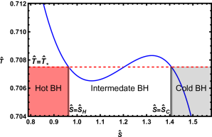
Figure 1: A typical $\hat{T}-\hat{S}$ diagram for $\hat{P}<\hat{P}_{c}$ ($\hat{P}=0.6$). A qualitatively similar diagram can be observed for pressures higher than its critical value, however, when the critical pressure is attained, the Maxwell areas vanish.

III Thermodynamic geometry

In this section, we employ a novel formalism of thermodynamic geometry, known as NTG Hosseini Mansoori and Mirza (2019), to explore the phase behavior of the system. This framework facilitates the identification of a direct mapping between phase transitions and singularities within the thermodynamic scalar curvature. The NTG geometry is characterized by

$$dl_{NTG}^{2}=\frac{1}{T}\left(\eta_{i}^{j}\,\frac{\partial^{2}\Xi}{\partial X^{j}\partial X^{l}}\,dX^{i}dX^{l}\right),$$ (17)

where $\eta_{i}^{j}={\rm diag}(-1,1,...,1)$, $\Xi$ is a thermodynamic potential and $X^{i}$ are intensive/extensive variables Hosseini Mansoori and Mirza (2019).

As mentioned before, the NTG results extend further our knowledge of phase transition points. For example, in the fixed central charge ensemble, as one chooses thermodynamic potential by Legendre transformation like $\Xi=H(S,P)=E+PV=M(S,P)$, the curvature singularity occurs exactly at the same location as the phase transition point of $C_{P,c}$ happens Hosseini Mansoori and Mirza (2019). In addition, this result holds true for conjugate potential pairs $(\Xi,\overline{\Xi})$ that satisfy the following relation Hosseini Mansoori (2021),

$$\Xi+\overline{\Xi}=2E-TS+PV,$$ (18)

Therefore, one can prove that the singularities of the scalar curvatures $R^{H}$ and $R^{F}$, associated with the conjugate pair $\Xi=M(S,P)=H(S,P)$ and $\bar{\Xi}=F(T,V)=E-TS=M-PV-TS$, respectively, correspond to the divergences of $C_{P,c}$. In addition, their associated metrics are negative of each other, i.e.

$$g^{NTG}_{H}=-J^{T}g^{NTG}_{F}J\hskip 14.22636pt\text{or}\hskip 14.22636ptdl^{2}(H)=-dl^{2}(F),$$ (19)

where $J$ is the Jacobian matrix defined as

$$J=\frac{\partial(T,V)}{\partial(S,P)}=\left(\begin{matrix}\Big{(}\frac{\partial T}{\partial S}\Big{)}_{P}&\Big{(}\frac{\partial T}{\partial P}\Big{)}_{S}\\ \Big{(}\frac{\partial V}{\partial S}\Big{)}_{P}&\Big{(}\frac{\partial V}{\partial P}\Big{)}_{S}\\ \end{matrix}\right).$$ (20)

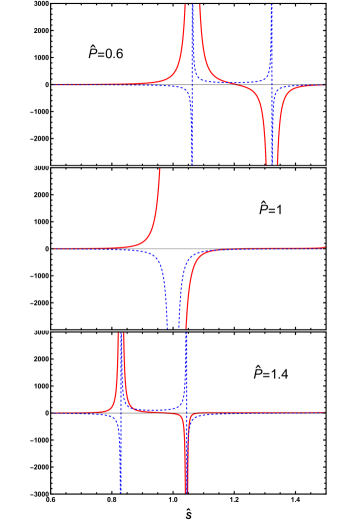
Figure 2: The diagram of the specific heat $C_{P,c}$ (blue dashed curve) and curvature $R^{H}$ (red curve) versus the entropy $\hat{S}$ for $\hat{P}=0.6$, $\hat{P}=1$, and $\hat{P}=1.4$. Note that the same figures can be obtained when one consider $R^{F}$.

Equipped with the enthalpy potential $M(S,P)$, we can employ NTG geometry to examine phase transition points of $C_{P,c}$. By substituting thermodynamic potential $\Xi=H=M=E+PV$ with $X^{i}=(S,P)$ into Eq. (17), we arrive at

$$g^{NTG}_{H}=\frac{1}{T}\text{diag}\left(M_{SS},-M_{PP}\right).$$ (21)

As all thermodynamic parameters are expressed as a function of $(z,\nu)$, it is convenient to transform the metric elements from the coordinate $X^{i}=(S,P)$ to the preferred coordinate $(z,\nu)$. To do this, we first need to redefine metric elements as follows,

$$M_{SS} = \frac{\partial^{2}M}{\partial S^{2}}=\left(\frac{\partial T}{\partial S}\right)_{P}=\frac{\{T,P\}_{z,\nu}}{\{S,P\}_{z,\nu}},$$ (22)

$$M_{PP} = \frac{\partial^{2}M}{\partial P^{2}}=\left(\frac{\partial V}{\partial P}\right)_{S}=\frac{\{V,S\}_{z,\nu}}{\{P,S\}_{z,\nu}},$$ (23)

then changing from coordinate $(S,P)$ to $(z,v)$ by using the below Jacobian matrix,

$$J_{c}=\frac{\partial(S,P)}{\partial(z,\nu)},$$ (24)

and finally convert the metric elements to

$$\hat{g}=J_{c}^{T}g^{NTG}_{M}J_{c}.$$ (25)

We have depicted the scalar curvature $R^{H}$ and heat capacity $C_{P,c}$ with respect to entropy in Fig. 2. It can be observed that there exists a one-to-one correspondence between the singularities of the Ricci scalar $R^{H}$ and the phase transition of $C_{P,c}$.

Fig. 2 also reveals that, for $P\neq P_{c}$ there exists two divergent points for $C_{P,c}$. The unstable phases with negative specific heat happen in the lower and higher entropy regions, while the intermediate phase with positive $C_{P,c}$ value is stable phase. As temperature is lower or higher than its critical value there are three possible phases, i.e., the cold black hole (CBH), intermediate black hole (IBH) and hot black hole (HBH). As temperature reaches to its critical value $T=T_{c}$, these two divergent points get closer and coincide at $\hat{S}=1$ to form a single divergence where the stable region disappears. It means that the black hole is unstable for $P=P_{c}$.

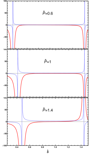
Figure 3: The diagram of the specific heat $C_{V,c}$ (blue dashed curve) and curvature $R^{G}$ (red curve) versus the entropy $\hat{S}$ for $\hat{P}=0.6$, $\hat{P}=1$, and $\hat{P}=1.4$. Note that the same figures can be obtined when one consider $R^{E}$.

Before proceeding to the next section, allow us to examine the correspondence between the phase transitions of $C_{V,c}$ and singularities of the NTG curvature. To construct the appropriate NTG metric elements, we need to select either $\Xi=E(S,V)=M-PV$ or $\bar{\Xi}=G(T,P)=E-TS+PV=H-TS$ in Eq. (17), with the coordinates $(S,V)$ and $(T,P)$, respectively. In Fig. 3, $C_{V,c}$ and $R^{G}$ have been depicted with respect to entropy. It is obvious that there exists a direct mapping between the phase transition points of $C_{V,c}$ and the singularities of $R^{G}$.

A notable finding is that both heat capacities $C_{V,c}$ and $C_{P,c}$ are positive within the intermediate black hole (coexistence) region, as illustrated in Figs. 2 and 3. This observation reinforces the argument put forth in Johnson (2020) regarding the significance of considering the signs of $C_{P,c}$ and $C_{V,c}$ in assessing the stability of black holes within the extended framework.

IV Coexistence curves and critical exponents

The aim of this section is to determine the critical exponents that describe the behavior of thermodynamic quantities such as heat capacities and thermodynamic curvatures, which were discussed in the previous section, near the critical point. In order to accomplish this, we construct the equal area law in the $\hat{T}-\hat{S}$ plane and then attempt to obtain the coexistence curve between the cold and hot black hole phases.

The coexistence phase in $\hat{T}-\hat{S}$ plane occurs within a range of entropy values determined using the Maxwell equal area construction, namely

$$\hat{T}_{\star}\Big{(}\hat{S}_{H}-\hat{S}_{C}\Big{)}=\int_{\hat{S}_{C}}^{\hat{S}_{H}}\hat{T}d\hat{S},$$ (29)

where $\hat{T}=\hat{T}_{\star}$ is the horizontal isothermal line. In this study, due to the complicated form of $T$, $S$, and $P$ (i.e., Eqs. (II), (2), and (4), respectively), it is not possible to express temperature explicitly in terms of $(S,P)$. However, we can determine temperature as a function of entropy at a constant pressure using numerical methods.

In Fig. 1, we have shown the location of $\hat{S}_{C}$ and $\hat{S}_{H}$ in the two black hole phases. Using Maxwell’s construction (29), we have further plotted the $\hat{P}-\hat{T}$ phase diagram in Fig. 4. This diagram features the two distinct black hole phases: cold and hot black holes. The red solid curve represents the coexistence phase. This curve originates from the origin, gradually increases with temperature, and ultimately terminates at the critical point, which is denoted by a black dot.

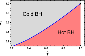
Figure 4: Phases of the qBTZ black hole. The blue solid curve is the coexistence curve of cold and hot black holes.

Furthermore, the entropy difference is considered as an order parameter in $\hat{T}-\hat{S}$ plane, which quantifies the phase change across the critical point, using the Maxwell equal-area law. Analogous to the Van der Waals fluid, we thus define

$$\eta=|\hat{S}_{H}-\hat{S}_{C}|.$$ (30)

Typically, near the critical point, the behavior of the entropy difference along the $\hat{P}-\hat{T}$ coexistence curve, is characterized by

$$\eta\sim\bigg{\{}\begin{matrix}(-t)^{\beta}&\hskip 14.22636pt\text{for}\hskip 14.22636ptt<0,\\ t^{\beta^{\prime}}&\hskip 14.22636pt\text{for}\hskip 14.22636ptt>0,\end{matrix}$$ (31)

where $t=\hat{T}-1$. Given the presence of a two-phase regime in the qBTZ system for either $t>0$ or $t<0$, it is reasonable to anticipate that the system exhibits identical critical behavior for both $t>0$ and $t<0$.

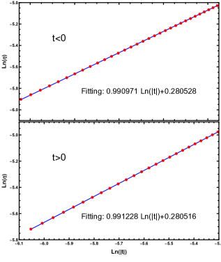
Figure 5: Diagram of $\ln\eta$ versus $\ln|t|$ on crossing the $\hat{P}-\hat{T}$ cold-hot coexistence curve of the qBTZ black hole. The fitted straight line for the data points (red dot) is given by $\eta=b(-t)^{\beta}$ with $b=1.32383$ and $\beta=0.990971$ for $t<0$ and $\eta=b^{\prime}t^{\beta^{\prime}}$ with $b^{\prime}=1.32381$ and $\beta^{\prime}=0.991228$ for $t>0$.

Fig. 5 presents the Ln-Ln plot of $\eta$ as a function of $t$ for $t\neq 0$. Form the slope and the intercept of the fitted straight lines for the numerical data points on the lower left with $|t|>10^{-4}$, we find

$$\eta\sim|t|\hskip 14.22636pt\text{for}\hskip 14.22636ptt\neq 0.$$ (32)

This shows that $\beta=\beta^{\prime}=1$. These exponent values significantly differ from the classical mean-field critical exponents for the van der Waals fluid Niu et al. (2012). In addition, the behavior of $C_{P,c}$ and $R^{H}$ along the coexistence curve and near the critical point are shown in Fig. 6. By increasing $\hat{T}$ for $\hat{T}<1$ or decreasing $\hat{T}$ for $\hat{T}>1$, both quantities decrease and diverge at the critical temperature $\hat{T}=1$. Near the critical point, one can consider the following critical behavior for $C_{P,c}$ and $R^{H}$ along $\hat{P}-\hat{T}$ coexistence curve.

$$\frac{C_{P,c}}{c}\sim\bigg{\{}\begin{matrix}(-t)^{-\alpha}&\hskip 14.22636pt\text{for}\hskip 14.22636ptt<0,\\ t^{-\alpha^{\prime}}&\hskip 14.22636pt\text{for}\hskip 14.22636ptt>0,\end{matrix}$$ (33)

and

$$R^{H}c\sim\bigg{\{}\begin{matrix}(-t)^{-\gamma}&\hskip 14.22636pt\text{for}\hskip 14.22636ptt<0,\\ t^{-\gamma^{\prime}}&\hskip 14.22636pt\text{for}\hskip 14.22636ptt>0.\end{matrix}$$ (34)

Employing Maxwell’s construction, we have studied the critical behaviour of $C_{P,c}$ and $R^{H}$ for $t>0$ and $t<0$ along $\hat{P}-\hat{T}$ coexistence curve, in Tab. 1.

Quantity	Coefficient	Temperature	SCBH	SHBH
		for $t<0$	2.013581	2.013420
	$c_{C}$	for $t>0$	2.014214	2.012750
$\ln(|C_{P,c}|)$		for $t<0$	1.794873	1.795891
	$d_{C}$	for $t>0$	1.787699	1.797094
		for $t<0$	3.013427	3.013230
	$c_{R}$	for $t>0$	3.010046	3.010006
$\ln(|R^{H}|)$		for $t<0$	-0.285991	-0.284792
	$d_{R}$	for $t<0$	-0.287398	-0.287158

Table 1: Fitting values of the slope and intercept of $\ln|C_{P,c}|=-c_{C}\ln(|t|)+d_{C}$ and $\ln|R^{H}|=-c_{R}\ln(|t|)+d_{R}$ straight line for coexistence saturated cold black hole (SCBH) and coexistence saturated hot black hole (SHBH) curves.

According to the data shown in Tab. 1, by taking numerical error into account, one finds that

$$\frac{C_{P,c}}{c}(-t)^{2} = -\exp\frac{(1.794873+1.795891)}{2}\approx-6.021,$$

$$\frac{C_{P,c}}{c}t^{2} = -\exp\frac{(1.787699+1.797094)}{2}\approx-6.003,$$

for $t<0$ and $t>0$, respectively. This implies $\alpha=\alpha^{\prime}=2$ which are are not mean field critical exponents Niu et al. (2012). Similarly, one obtains

$$R^{H}c(-t)^{3} = -\exp\frac{(-0.285991-0.284792)}{2}\approx-0.75171,$$

$$R^{H}ct^{3} = -\exp\frac{(-0.287398-0.287158)}{2}\approx-0.75030.$$

The above relations reveal that $\gamma=\gamma^{\prime}=3$. As a result, we have

$$\frac{C_{P,c}}{c}|t|^{2}\approx-6\hskip 8.5359pt\text{and}\hskip 8.5359ptR^{H}c|t|^{3}\approx-\frac{3}{4}\hskip 14.22636pt\text{for}\hskip 14.22636ptt\neq 0.$$ (35)

Interestingly, the critical amplitudes are dimensionless constants and independent of the central charge. In addition, thanks to $dl_{H}^{2}=-dl_{F}^{2}$, we can conclude

$$R^{F}C^{\rm qBTZ}_{V}|t|^{3}\approx-2\hskip 14.22636pt\text{for}\hskip 14.22636ptt\neq 0.$$ (36)

where the heat capacity takes the positive finite value, i.e., $C^{\rm qBTZ}_{V}\approx 64c\pi/75$ near the critical point. Furthermore, Eq. (36) indicates a continuity in the criticality of thermodynamic curvature as we approach to the critical point for $t\to 0^{\pm}$ limits.

This finding is significantly differ from the result reported in Hosseini Mansoori et al. (2020); Wei et al. (2019a) for a VdW fluid. In the VdW fluid case, we observe two-phase regime (the liquid/gas phase) only for $t<0$. Therefore, for $t<0$ we get close to the critical point along coexistence line between the liquid phase and the gas phase, whereas for $t>0$ we approach to the critical point along the isochore line $v=v_{c}$ ($v$ is the specific volume) in $P-v$ plane. Consequently, our choice of various trajectories in $P-v$ diagram on approaching to the critical point leads to a discontinuity in criticality of the NTG curvature, that is,

$$R^{F}C^{\rm VdW}_{V}|t|^{2}\approx\bigg{\{}\begin{matrix}-\frac{1}{8}&\text{for}\hskip 14.22636ptt<0,\\ -\frac{1}{2}&\text{for}\hskip 14.22636ptt>0,\\ \end{matrix}$$ (37)

where $C^{\rm VdW}_{V}=3/2$ when one takes $k_{B}=1$ Hosseini Mansoori et al. (2020); Wei et al. (2019a).

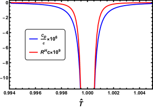
Figure 6: The behaviour of $C_{P}$ and $R^{H}$ along the coexistence saturated cold curve. The same figure will be obtained for the coexistence saturated hot curve.

V Conclusions

In this paper we have carried out a thorough exploration of the critical behavior and extended phase structure of the quantum BTZ black hole. This solution was discovered via braneworld holography, and embodies the semiclassical backreaction effects of quantum conformal matter onto the geometry. Consequently, it serves as a holographic dual to a finite-$N$ quantum field theory.

Focusing on the fixed central charge ensemble, we first revisited the derivation of the heat capacities $C_{P,c}$ and $C_{V,c}$ using the bracket method introduced in Mansoori et al. (2015). Subsequently, we illustrated the phase structure of the qBTZ black hole in the $T-S$ plane. Notably, our analysis revealed a two-phase regime at both low and high temperature limits. Intriguingly, except for a critical pressure, $P=P_{c}$, the heat capacity $C_{P,c}$ undergoes a sign change at two phase transition points, indicative of the system transitioning between stable and unstable branches. Remarkably, $C_{V,c}$ remains positive at these points, allowing the system to seamlessly transfer between these branches.

Utilizing the NTG geometry, we then formulated a metric to accurately represent the one-to-one relationship between phase transitions of heat capacities and the singularities of scalar curvatures. Employing this framework, we examined the critical behavior of heat capacities and scalar curvatures near the critical point. Specifically, we numerically assessed the criticality of such curvature along the coexistence curve in the $\hat{T}-\hat{S}$ diagram as it approached the critical point.

Our findings revealed that the critical exponent of $C_{P,c}$ and the scalar curvature $R^{H}$ are 2 and 3, respectively, diverging from the well-known critical mean-field values for Van der Waals fluids. Other gravitational systems exhibiting non-standard critical exponents include the so-called Lovelock black holes Frassino et al. (2014, 2016). It would be interesting to understand more broadly the circumstances and mechanisms wherein mean field theory predictions may be circumvented. Notably, our numerical data unveiled that critical amplitudes remain unaffected by the central charge in the qBTZ black hole. This prompts an intriguing inquiry into their potential universality, which could be explored further by investigating other quantum black holes, such as the charged quantum BTZ Climent et al. , and the quantum Schwarzschild-de Sitter and Kerr-de Sitter solutions in three dimensions Emparan et al. (2022); Panella and Svesko (2023). We defer such investigation for future examination.

Acknowledgements. We are grateful to Roberto Emparan, Antonia Frassino and Andrew Svesko for useful discussions and correspondence. JFP is supported by the ‘Atracción de Talento’ program grant 2020-T1/TIC-20495, the Spanish Research Agency through the grants CEX2020-001007-S and PID2021-123017NB-I00, funded by MCIN/AEI/10.13039/501100011033 and by ERDF A way of making Europe.

Appendix A Partial derivatives and bracket notation

Let us introduce the bracket method for doing partial derivatives. This allows us to calculate heat capacities very easily. Generally, if we consider $f$, $g$, and $h$ as explicit functions of $(a,b)$, the partial derivative can be expressed by Poisson bracket as follows Mansoori et al. (2015):

$$\Big{(}\frac{\partial f}{\partial g}\Big{)}_{h}=\frac{\{f,h\}_{a,b}}{\{g,h\}_{a,b}}$$ (38)

where $\{.,.\}$ is Poisson bracket given by

$$\{f,g\}_{a,b}=\Big{(}\frac{\partial f}{\partial a}\Big{)}_{b}\Big{(}\frac{\partial g}{\partial b}\Big{)}_{a}-\Big{(}\frac{\partial f}{\partial b}\Big{)}_{a}\Big{(}\frac{\partial g}{\partial a}\Big{)}_{b}$$ (39)

Moreover, we can generalize the bracket method for functions depending on $(n+1)$ independent variables. In this case, the partial derivative can be expressed as Mansoori et al. (2015)

$$\Big{(}\frac{\partial f}{\partial g}\Big{)}_{h_{1},h_{2},...,h_{n}}=\frac{\{f,h_{1},h_{2},...,h_{n}\}_{q_{1},q_{2},...,q_{n+1}}}{\{g,h_{1},h_{2},...,h_{n}\}_{q_{1},q_{2},...,q_{n+1}}}$$ (40)

where all $f$, $g$, and $h_{n}$ ($n=1,2,3,...$) are functions of $q_{i}$, $i=1,2,...,n+1$ independent variables and $\{.,.,.\}$ denotes Nambu bracket that is defined as,

$$\{f,h_{1},...,h_{n}\}_{q_{1},...,q_{n+1}}=\sum_{ijk...l=1}^{n+1}\epsilon_{ijk...l}\frac{\partial f}{\partial q_{i}}\frac{\partial h_{1}}{\partial q_{j}}\frac{\partial h_{2}}{\partial q_{k}}...\frac{\partial h_{n}}{\partial q_{l}}$$ (41)

where $\epsilon_{ijk..l}$ is the Levi-Civita symbol.

References

- Kastor et al. (2009) D. Kastor, S. Ray, and J. Traschen, Class. Quant. Grav. 26, 195011 (2009), arXiv:0904.2765 [hep-th] .
- Dolan (2011) B. P. Dolan, Class. Quant. Grav. 28, 125020 (2011), arXiv:1008.5023 [gr-qc] .
- Cvetic et al. (2011) M. Cvetic, G. W. Gibbons, D. Kubiznak, and C. N. Pope, Phys. Rev. D 84, 024037 (2011), arXiv:1012.2888 [hep-th] .
- Kubiznak and Mann (2012) D. Kubiznak and R. B. Mann, JHEP 07, 033 (2012), arXiv:1205.0559 [hep-th] .
- Kubiznak and Mann (2015) D. Kubiznak and R. B. Mann, Can. J. Phys. 93, 999 (2015), arXiv:1404.2126 [gr-qc] .
- Altamirano et al. (2013) N. Altamirano, D. Kubiznak, and R. B. Mann, Phys. Rev. D 88, 101502 (2013), arXiv:1306.5756 [hep-th] .
- Altamirano et al. (2014a) N. Altamirano, D. Kubizňák, R. B. Mann, and Z. Sherkatghanad, Class. Quant. Grav. 31, 042001 (2014a), arXiv:1308.2672 [hep-th] .
- Altamirano et al. (2014b) N. Altamirano, D. Kubiznak, R. B. Mann, and Z. Sherkatghanad, Galaxies 2, 89 (2014b), arXiv:1401.2586 [hep-th] .
- Johnson (2014) C. V. Johnson, Class. Quant. Grav. 31, 205002 (2014), arXiv:1404.5982 [hep-th] .
- Dolan (2014) B. P. Dolan, JHEP 10, 179 (2014), arXiv:1406.7267 [hep-th] .
- Wei and Liu (2013) S.-W. Wei and Y.-X. Liu, Phys. Rev. D 87, 044014 (2013), arXiv:1209.1707 [gr-qc] .
- Cai et al. (2013) R.-G. Cai, L.-M. Cao, L. Li, and R.-Q. Yang, JHEP 09, 005 (2013), arXiv:1306.6233 [gr-qc] .
- Sherkatghanad et al. (2016) Z. Sherkatghanad, B. Mirza, Z. Mirzaiyan, and S. A. Hosseini Mansoori, Int. J. Mod. Phys. D 26, 1750017 (2016), arXiv:1412.5028 [gr-qc] .
- Caceres et al. (2015) E. Caceres, P. H. Nguyen, and J. F. Pedraza, JHEP 09, 184 (2015), arXiv:1507.06069 [hep-th] .
- Karch and Robinson (2015) A. Karch and B. Robinson, JHEP 12, 073 (2015), arXiv:1510.02472 [hep-th] .
- Pedraza et al. (2019) J. F. Pedraza, W. Sybesma, and M. R. Visser, Class. Quant. Grav. 36, 054002 (2019), arXiv:1807.09770 [hep-th] .
- Visser (2022) M. R. Visser, Phys. Rev. D 105, 106014 (2022), arXiv:2101.04145 [hep-th] .
- Amo et al. (2023) M. Amo, A. M. Frassino, and R. A. Hennigar, Phys. Rev. Lett. 131, 241401 (2023), arXiv:2307.03011 [gr-qc] .
- Kubiznak et al. (2017) D. Kubiznak, R. B. Mann, and M. Teo, Class. Quant. Grav. 34, 063001 (2017), arXiv:1608.06147 [hep-th] .
- Ruppeiner (1979) G. Ruppeiner, Physical Review A 20, 1608 (1979).
- Oshima et al. (1999) H. Oshima, T. Obata, and H. Hara, Journal of Physics A: Mathematical and General 32, 6373 (1999).
- Ruppeiner (1995) G. Ruppeiner, Reviews of Modern Physics 67, 605 (1995).
- Åman et al. (2003) J. E. Åman, I. Bengtsson, and N. Pidokrajt, General Relativity and Gravitation 35, 1733 (2003).
- Mirza and Zamaninasab (2007) B. Mirza and M. Zamaninasab, Journal of High Energy Physics 2007, 059 (2007).
- Mansoori and Mirza (2014) S. A. H. Mansoori and B. Mirza, Eur. Phys. J. C 74, 2681 (2014), arXiv:1308.1543 [gr-qc] .
- Hosseini Mansoori and Mirza (2019) S. A. Hosseini Mansoori and B. Mirza, Phys. Lett. B 799, 135040 (2019), arXiv:1905.01733 [gr-qc] .
- Mansoori et al. (2016) S. A. H. Mansoori, B. Mirza, and E. Sharifian, Phys. Lett. B 759, 298 (2016), arXiv:1602.03066 [gr-qc] .
- Mansoori et al. (2015) S. A. H. Mansoori, B. Mirza, and M. Fazel, JHEP 04, 115 (2015), arXiv:1411.2582 [gr-qc] .
- Sarkar et al. (2006) T. Sarkar, G. Sengupta, and B. Nath Tiwari, JHEP 11, 015 (2006), arXiv:hep-th/0606084 .
- Hosseini Mansoori et al. (2020) S. A. Hosseini Mansoori, M. Rafiee, and S.-W. Wei, Phys. Rev. D 102, 124066 (2020), arXiv:2007.03255 [gr-qc] .
- Rafiee et al. (2022) M. Rafiee, S. A. H. Mansoori, S.-W. Wei, and R. B. Mann, Phys. Rev. D 105, 024058 (2022), arXiv:2107.08883 [gr-qc] .
- Wei et al. (2019a) S.-W. Wei, Y.-X. Liu, and R. B. Mann, Phys. Rev. Lett. 123, 071103 (2019a), arXiv:1906.10840 [gr-qc] .
- Wei et al. (2019b) S.-W. Wei, Y.-X. Liu, and R. B. Mann, Phys. Rev. D 100, 124033 (2019b), arXiv:1909.03887 [gr-qc] .
- Emparan et al. (2020) R. Emparan, A. M. Frassino, and B. Way, JHEP 11, 137 (2020), arXiv:2007.15999 [hep-th] .
- Randall and Sundrum (1999a) L. Randall and R. Sundrum, Phys. Rev. Lett. 83, 4690 (1999a), arXiv:hep-th/9906064 .
- Randall and Sundrum (1999b) L. Randall and R. Sundrum, Phys. Rev. Lett. 83, 3370 (1999b), arXiv:hep-ph/9905221 .
- Karch and Randall (2001a) A. Karch and L. Randall, JHEP 05, 008 (2001a), arXiv:hep-th/0011156 .
- Karch and Randall (2001b) A. Karch and L. Randall, JHEP 06, 063 (2001b), arXiv:hep-th/0105132 .
- de Haro et al. (2001) S. de Haro, K. Skenderis, and S. N. Solodukhin, Classical and Quantum Gravity 18, 3171 (2001).
- Emparan et al. (2000a) R. Emparan, G. T. Horowitz, and R. C. Myers, JHEP 01, 007 (2000a), arXiv:hep-th/9911043 .
- Emparan et al. (2000b) R. Emparan, G. T. Horowitz, and R. C. Myers, JHEP 01, 021 (2000b), arXiv:hep-th/9912135 .
- Emparan et al. (2002) R. Emparan, A. Fabbri, and N. Kaloper, JHEP 08, 043 (2002), arXiv:hep-th/0206155 .
- Frassino et al. (2023a) A. M. Frassino, J. F. Pedraza, A. Svesko, and M. R. Visser, Phys. Rev. Lett. 130, 161501 (2023a), arXiv:2212.14055 [hep-th] .
- Kudoh and Kurita (2004) H. Kudoh and Y. Kurita, Phys. Rev. D 70, 084029 (2004), arXiv:gr-qc/0406107 .
- Johnson and Nazario (2023) C. V. Johnson and R. Nazario, (2023), arXiv:2310.12212 [hep-th] .
- Frassino et al. (2023b) A. M. Frassino, J. F. Pedraza, A. Svesko, and M. R. Visser, (2023b), arXiv:2310.12220 [hep-th] .
- Hosseini Mansoori (2021) S. A. Hosseini Mansoori, Phys. Dark Univ. 31, 100776 (2021), arXiv:2003.13382 [gr-qc] .
- Johnson (2020) C. V. Johnson, Mod. Phys. Lett. A 35, 2050098 (2020), arXiv:1906.00993 [hep-th] .
- Niu et al. (2012) C. Niu, Y. Tian, and X.-N. Wu, Phys. Rev. D 85, 024017 (2012), arXiv:1104.3066 [hep-th] .
- Frassino et al. (2014) A. M. Frassino, D. Kubiznak, R. B. Mann, and F. Simovic, JHEP 09, 080 (2014), arXiv:1406.7015 [hep-th] .
- Frassino et al. (2016) A. M. Frassino, R. B. Mann, and F. Simovic, in 2nd Karl Schwarzschild Meeting on Gravitational Physics (2016) arXiv:1611.03525 [hep-th] .
- (52) A. Climent, R. Emparan, and R. Hennigar, to appear.
- Emparan et al. (2022) R. Emparan, J. F. Pedraza, A. Svesko, M. Tomašević, and M. R. Visser, JHEP 11, 073 (2022), arXiv:2207.03302 [hep-th] .
- Panella and Svesko (2023) E. Panella and A. Svesko, JHEP 06, 127 (2023), arXiv:2303.08845 [hep-th] .