Shadows of black holes in dynamical Chern-Simons modified gravity

Abstract

We revisit and extend the study of null geodesics around a slowly rotating black hole in Chern-Simons modified gravity. We employ the Hamilton-Jacobi formalism to derive the equations for the shadow profile and determine its shape. We compare our results with numerical ray tracing, finding good agreement within the validity of our approximations for slow rotation and small Chern-Simons coupling. We constrain the model parameters using data from the observed shadow of SgrA^∗.

1 Abstract

Contents

1. 1 Abstract
2. 2 Introduction
3. 3 Formulation of Chern-Simons modified gravity
4. 4 Hamilton-Jacobi Formalism in General Relativity
   1. 4.1 Hamilton-Jacobi equations in Kerr space-time
   2. 4.2 Shadow of the Kerr black hole
5. 5 Black holes in dCS modified gravity: slow rotation approximation
   1. 5.1 Hamilton-Jacobi equations in dCS and Separation of Variables.
   2. 5.2 Shadows of dCS black holes
   3. 5.3 Images of dCS black hole with accretion disk
   4. 5.4 Observables for the shadow
6. 6 Discussion
7. 7 Acknowledgments

2 Introduction

In 1915, Albert Einstein formulated the General Theory of Relativity (GR), which relates gravity to the geometry of space-time. This theory has been extensively tested on the Solar System and other astrophysical scales [Will_2014] and is the basis of the Standard Cosmological Model. However; unless some exotic energy/matter content is considered, a few observations and theoretical questions elude GR’s explanations, such as the late acceleration of the Universe [Perlmutter_1999,Riess_1998] and the anomalous rotation curves of galaxies [Sofue_2001]. Modifying GR offers alternative ways to address these unresolved issues, but any modification must reproduce well-tested predictions of GR. One such prediction, which has gained observational relevance in recent years, is the appearance of photons orbiting in unstable orbits around a black hole in an observer’s sky, the black hole shadow [Stepanian_2021,Ayzenberg_2018,PhysRevD.106.064012,Antoniou_2023].

A reason for the recent surge in black hole research is the reconstruction by the Event Horizon Telescope (EHT) of the first image of the shadow of the Supermassive Black Hole (SMBH) in the center of the $M87^{*}$ galaxy in 2019 [Akiyama_2019], followed by the image of the shadow of Sagittarius $A^{*}$, located in the center of the Milky Way [2022ApJ…930L..12E], also reported by the EHT in 2022. This opens up new possibilities for constraining modified theories of gravity, since the size of the shadow can be affected both by the new coupling constants introduced by the alternative model of gravity and by the properties of the black hole solution, which usually is not the same as in GR.

In this work, we focus on shadows of black holes within modifications to GR that introduce a scalar field non-minimally coupled to squared curvature scalars, commonly known as quadratic gravity theories [Yunes_2011]. In particular, we work in the theory known as dynamical Chern-Simons gravity (dCS) [Jackiw_2003]. Several aspects of dCS have been explored in the literature. Cosmological studies have explored its connection with cosmic microwave background radiation [Lue_1999,Li_2007] and leptogenesis [Alexander_2006,Alexander_200]. Gravitational wave solutions have also been investigated in [Yunes_2010,Wagle_2022,Yagi_2012].

Concerning black hole solutions in dCS [Wagle_2022,Grumiller_20008,PhysRevLett.28.1082,erdmenger2022universal,Kimura_2018], spherically symmetric spacetimes known in GR persist as solutions in dCS, whereas axially symmetric solutions do not. Yunes and Pretorious [Yunes_2009] reported the first solution that describes a rotating black hole in the slow rotation/small coupling limit. This solution introduces a modification to the Kerr metric parameterized by a scalar hair, resulting in a correction to the location of photon orbits. An analysis of these corrections was presented in [PhysRevD.81.124045]. In this work, we revisit and expand on these results, also presenting numerical shadows with an accretion disk and using observational data from M87^∗ and SgrA^∗ to put constraints on the parameters of dCS spacetime.

This paper is organized as follows. In Section 3 we present the basics of the dynamical Chern-Simons theory. In Section 4 we review the Hamilton-Jacobi formalism to investigate the shadow of the Kerr black hole in GR. In Section 5 we apply the Hamilton-Jacobi formalism to the slowly rotating black hole found in dynamical Chern-Simons gravity, and we also present images generated with the ray-tracing code Gyoto. We investigate the radius of the shadow and the distortion with respect to a Kerr black hole. These observable parameters allow us to compare the predictions of dCS with the observations reported by EHT. We conclude in Section 6 with a discussion of our results.

3 Formulation of Chern-Simons modified gravity

Chern-Simons modified gravity (CS) represents a 4-dimensional deformation of GR defined by the action

$$S_{total}=S_{EH}+S_{CS}+S_{\vartheta}+S_{mat}.$$ (1)

The first term is the Einstein-Hilbert action,

$$S_{EH}=\kappa\int d^{4}x\sqrt{-g}R,$$ (2)

where $\kappa=\left(16\pi\right)^{-1}$ is the dimensionless gravitational coupling constant in units $c=G=1$, $R$ is the Ricci scalar, and $g$ is the determinant of the metric $g_{\mu\nu}$.

The CS term is given by

$$S_{CS}=\frac{\alpha}{4}\int d^{4}x\sqrt{-g}\vartheta{}^{\star}\!RR,$$ (3)

where $\alpha$ is the CS coupling constant with units of length squared, ${}^{\star}\!R$ is the dual Riemann tensor used to form the Pontryagin density ${}^{\star}\!RR$, and $\vartheta$ is a dimensionless scalar field, known as the Chern-Simons coupling field. In components,

$${}^{\star}RR ={}^{\star}R^{\mu}{}_{\nu}{}^{\rho\sigma}R^{\nu}{}_{\mu}{}_{\rho\sigma}=\frac{1}{2}\epsilon^{\rho\sigma\delta\tau}R^{\mu}{}_{\nu}{}_{\delta\tau}R^{\nu}{}_{\mu}{}_{\rho\sigma}.$$ (4)

with $\epsilon^{\rho\sigma\delta\tau}$ being the 4-dimensional Levi-Civita tensor,

The scalar field action is given by

$$S_{\vartheta}=-\frac{\beta}{2}\int d^{4}x\sqrt{-g}\left[g^{\mu\nu}\nabla_{\mu}\vartheta\nabla_{\nu}\vartheta+2V(\vartheta)\right],$$ (5)

where $\nabla_{\mu}$ is the covariant derivative compatible with the metric, $\beta$ is a dimensionless coupling constant, and $V(\vartheta)$ is a potential for the scalar that we set to zero.

An additional, unspecified matter contribution is described by

$$S_{mat}=\frac{1}{4}\int d^{4}x\sqrt{-g}\mathcal{L}_{mat},$$ (6)

where $\mathcal{L}_{mat}$ is a Lagrangian density that does not depend on $\vartheta$. The modified CS equations include a variety of theories, each characterized by specific couplings $\alpha$ and $\beta$. Within this family, two distinct formulations stand out: the non-dynamical framework, where $\alpha$ can take any value while $\beta=0$, and the dynamical framework, where both $\alpha$ and $\beta$ are arbitrary but nonzero. Unfortunately, since its inception, this theory has been explored with various notations for the coupling constants, here we adhere to the notation used in Ref. [Alexander_2009].

If the scalar field $\vartheta$ is a constant, then the CS modified gravity reduces identically to GR. This occurs because the Pontryagin term (4) can be expressed as a divergence,

$$\nabla_{\mu}K^{\mu}=\frac{1}{2}{}^{\star}RR,$$ (7)

of the Chern-Simons topological current

$$K^{\mu}=\epsilon^{\mu\rho\sigma\tau}\Gamma^{\upsilon}_{\rho\psi}\left(\partial_{\sigma}\Gamma^{\psi}_{\tau\upsilon}+\frac{2}{3}\Gamma^{\psi}_{\sigma\xi}\Gamma^{\xi}_{\tau\upsilon}\right),$$ (8)

where $\Gamma^{\psi}_{\sigma\xi}$ are the Christoffel symbols. Therefore, we focus on a non-constant $\vartheta$.

The field equations are obtained by varying the action with respect to the metric and the CS coupling field. The former leads to

$$G_{\mu\nu}+\frac{\alpha}{\kappa}C_{\mu\nu}=\frac{1}{2\kappa}T_{\mu\nu},$$ (9)

where $G_{\mu\nu}$ is the Einstein tensor and $C_{\mu\nu}$ is the trace-free C-tensor

$$C^{\mu\nu}=\left(\nabla_{\sigma}\vartheta\right)\epsilon^{\sigma\delta\alpha(\mu}\nabla_{\alpha}R^{\nu)}{}_{\delta}+\left(\nabla_{\sigma}\nabla_{\delta}\vartheta\right){}^{\star}\!R^{\delta(\mu\nu)\sigma}.$$ (10)

On the other hand, variation with respect to the CS coupling field leads to

$$\beta\Box\vartheta=-\frac{\alpha}{4}\,{}^{\star}\!RR,$$ (11)

where $\Box:=g^{\mu\nu}\nabla_{\mu}\nabla_{\nu}$ is the d’Alembert operator. The previous is the Klein-Gordon equation for a massless scalar field in the presence of a source term.

4 Hamilton-Jacobi Formalism in General Relativity

Much can be learned from the study of the geodesics of massive particles and photons around black holes, contributing to a deeper comprehension of the physics of space-time. For an analytical examination of these trajectories, the Hamilton-Jacobi formalism proves advantageous, and we provide a brief overview here. This will serve as a foundation for our subsequent exploration of geodesics in the dCS metric.

The space-time geometry in GR for a rotating black hole is described by the Kerr metric [PhysRevLett.11.237]. According to GR, the exterior region of stellar and supermassive black holes is characterized by this metric. In Boyer-Lindquist coordinates $(t,r,\theta,\phi)$, this metric takes the form:

$$ds^{2} =-\left(1-\frac{2mr}{\rho^{2}}\right)dt^{2}-\frac{4mr\sin^{2}{\theta}}{\rho^{2}}dtd\phi+\frac{\rho^{2}}{\Delta}dr^{2}+\rho^{2}d\theta^{2}+\sin^{2}{\theta}d\Omega,$$ (12)

where

$$d\Omega=\left(r^{2}+a^{2}+\frac{2mar\sin^{2}{\theta}}{\rho^{2}}\right)d\phi^{2},$$ (13)

where $m$ is the mass in geometrized units , and $\rho^{2}$ and $\Delta$ are defined as

$$\rho^{2}=r^{2}+a^{2}\cos^{2}{\theta},$$ (14)

$$\Delta=r^{2}+a^{2}-2mr.$$ (15)

The parameter $a$ measures the specific angular momentum [ryder_2009]. To prevent a naked singularity, observable from infinity and forbidden by the cosmic censorship conjecture [carroll1997lecture], the value of $a$ is restricted to the interval $a\in[-m,m]$, or equivalently $\left|a\right|\leq m$.

4.1 Hamilton-Jacobi equations in Kerr space-time

The Hamiltonian for a particle in spacetime is expressed as

$$H=\frac{1}{2}g^{\mu\nu}p_{\mu}p_{\nu},$$ (16)

where $p_{\mu}$ are the generalized momenta. From the Hamilton-Jacobi formulation, this leads to

$$\frac{\partial S}{\partial\lambda}=-\frac{1}{2}g^{\mu\nu}\frac{\partial S}{\partial x^{\mu}}\frac{\partial S}{\partial x^{\nu}}.$$ (17)

where $S$ is the Hamilton’s principal function. In Kerr space-time, due to the symmetry of the problem, $H$ does not explicitly depend on $t$, $\phi$, and the affine parameter $\lambda$, resulting in three linear terms in $S$. Furthermore, it is assumed that the radial and angular dependencies are also separable. Then, the function $S$ is proposed as

$$S=\frac{\mu^{2}}{2}\lambda+Et+\Phi\phi+S_{r}(r)+S_{\theta}(\theta),$$ (18)

where

$$\frac{\partial S}{\partial\lambda}=-H=\frac{\mu^{2}}{2},$$ (19)

and $\mu$ is the rest mass of the particle in geometrized units. The conserved quantities $E=-p_{t}$ and $\Phi=p_{\varphi}$ correspond to the specific energy and axial component of the angular momentum relative to an observer at infinity. Substituting Eq. (18) into the Hamilton-Jacobi Eq. (17) , we have

$$g^{tt}E^{2}+g^{\varphi\varphi}\Phi^{2}-2g^{t\varphi}E\Phi+g^{rr}\left(\frac{dS_{r}}{dr}\right)^{2}+g^{\theta\theta}\left(\frac{dS_{\theta}}{d\theta}\right)^{2}=-\mu^{2}.$$ (20)

Substituting the inverse terms of the Kerr metric and simplifying, we obtain

$$\frac{-P^{2}+p^{2}_{r}\Delta^{2}+\Delta r^{2}\mu^{2}}{\Delta}= -\left[a^{2}\mu^{2}\cos^{2}{\theta}+\left(aE\sin{\theta}-\frac{\Phi}{\sin\theta}\right)^{2}+p^{2}_{\theta}\right],$$ (21)

where $P=E(r^{2}+a^{2})-a\Phi$, $p_{r}={\partial S}/{\partial r}$, and $p_{\theta}={\partial S}/{\partial\theta}$. The left hand side depends solely on the coordinate $r$ and is defined as $f_{r}(r)$, while the right hand side depends only on $\theta$ and is defined as $f_{\theta}(\theta)$. Therefore, the equality in Eq. (21) implies that both sides are equal to a constant, which we define as

$$f_{r}(r)=f_{\theta}(\theta)=-K.$$ (22)

Sometimes, these equations are expressed in terms of the conserved quantity

$$Q=K-(aE-\Phi)^{2},$$ (23)

called Carter’s constant. In terms of this quantity, it can be written as

$$\Delta^{2}p^{2}_{r}=P^{2}-\Delta[Q+(aE-\Phi)^{2}+\mu^{2}r^{2}].$$

Using $\dot{r}=p^{r}=g^{rr}p_{r}={\Delta}p_{r}/{\rho^{2}}$, we obtain the equation of motion for $r$ as

$$\rho^{2}\dot{r}=\pm\sqrt{P^{2}-\Delta[Q+(aE-\Phi)^{2}+\mu^{2}r^{2}]}=\pm\sqrt{R(r)}.$$ (24)

Similarly, the equation for $\theta$ is obtained from $-K=f_{\theta}(\theta)$ and $\dot{\theta}=g^{\theta\theta}p_{\theta}={p_{\theta}}/{\rho^{2}}$, arriving to

$$\rho^{2}\dot{\theta}=\sqrt{Q-\cos^{2}{\theta}\left(a^{2}(\mu^{2}-E^{2})+\frac{\Phi^{2}}{\sin^{2}{\theta}}\right)}=\sqrt{\Theta(\theta)}.$$ (25)

The orbits of the test particles in Kerr geometry are obtained from the solutions to Eqs. (24) and (25). For photons, $\mu=0$, the equations of motion for $r$ and $\theta$ become

$$\rho^{4}\dot{r}^{2} =R(r)=P^{2}-\Delta\left(Q+(aE-\Phi)^{2}+\mu^{2}r^{2}\right),$$ (26)

$$\rho^{4}\dot{\theta}^{2} =\Theta(\theta)=Q-\cos^{2}{\theta}\left(a^{2}(\mu^{2}-E^{2})+\frac{\Phi^{2}}{\sin^{2}{\theta}}\right).$$ (27)

Dividing the equation of motion for $r$ by $E^{2}$ and using the reduced Carter constants $\lambda={\Phi}/{E},\eta={Q}/{E^{2}}$ we get

$$\Re(r)=\frac{R(r)}{E^{2}}=r^{4}+(a^{2}-\eta-\lambda^{2})r^{2}+2mr[\eta+(a-\lambda)^{2}]-\eta a^{2}.$$ (28)

The conditions for spherical orbits [PhysRevD.5.814,Fathi,Teo_2021,Perlick_2017] are then given by

$$\Re=0,\ \ \ \frac{d\Re}{dr}=0.$$ (29)

The solution to this set of equations is provided by the roots of a quadratic equation. Each of these two roots leads to a different class of solutions, and only one of these classes corresponds to physically viable spherical orbits. In this class, it follows from Eq. (29) that

$$\lambda =-\frac{r^{3}-3mr^{2}+a^{2}r+ma^{2}}{a(r-m)},$$ (30)

$$\eta =-\frac{r^{3}(r^{3}-6mr^{2}+9m^{2}r-4a^{2}m)}{a^{2}(r-m)^{2}}.$$ (31)

Even though $\lambda$ and $\eta$ are expressed in terms of the orbital radius, for a photon following a geodesic, these quantities remain constant. It is worth mentioning that these spherical orbits are unstable.

For Eqs. (30) and (31), the condition $\eta\geq 0$ [Chandrasekhar:1985kt] restricts the range of the radial coordinate to $r_{1}\leq r\leq r_{2}$, where $r_{1}$ and $r_{2}$ are the roots of $\eta$,

$$r_{1}=2m\left[1+2\cos\left(\frac{2}{3}\arccos{\theta}\left[-\frac{|a|}{m}\right]\right)\right],$$ (32)

$$r_{2}=2m\left[1+2\cos\left(\frac{2}{3}\arccos{\theta}\left[\frac{|a|}{m}\right]\right)\right].$$ (33)

It turns out that $r_{1}$ is associated with a rotating orbit and $r_{2}$ with a counter-rotating orbit , see Figure 1.

4.2 Shadow of the Kerr black hole

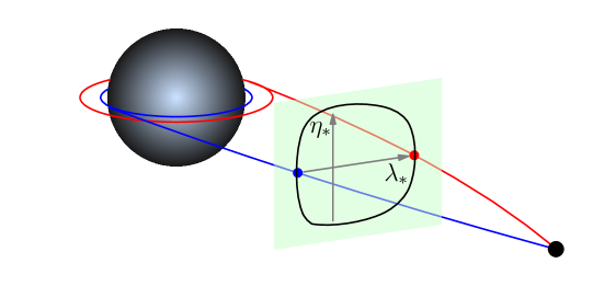
Figure 1: Two unstable circular orbits in the equatorial plane of a Kerr black hole (figure based on [35]). The one with the smaller radius is rotating the blue orbit, and the one with the larger radius is counterrotating the red orbit. Light rays asymptotically approaching them give two points on the shadow boundary curve for an observer in the equatorial plane. The spherical orbits of light outside the equatorial plane are not flat.

The formation of the black hole shadow is primarily influenced by the gravitational bending of light. To analyse this phenomenon one must consider the perspective of an observer positioned at a certain distance from the black hole [1979A&A….75..228L,10.1093/mnras/131.3.463,Bardeen:1973tla,Chandrasekhar:1985kt,Brihaye_2017,Perlick_2022,alma991019795519703414,Grenzebach_2014,Grenzebach_2015,Johannsen_2010]. The observable shape of a black hole is defined by the boundary of its shadow. When discussing this shadow, we use celestial coordinates as outlined in Ref. [Vázquez_Esteban_2004]. Specifically, we consider a scenario where the observer’s perspective aligns in such a way that the line of sight coincides with the equatorial plane of the black hole. In this configuration, the inclination angle of the observer is $\theta_{0}=\pi/2$ and the celestial coordinates are

$$\lambda*=-\lambda,\ \ \ \eta*=\sqrt{\eta}.$$ (34)

The coordinate $\lambda*$ represents the apparent horizontal distance of the image as seen from the symmetry axis, and the coordinate $\eta*$ is the apparent distance perpendicular to the equatorial plane, as illustrated in Fig. 1. Some examples of shadows for the Kerr black hole are presented in Fig. 2 for a distant equatorial observer ($r\gg m$, $\theta_{O}=\pi/2$) considering different values of spin $a=0,0.1,0.3,0.5,0.99$.

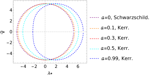
Figure 2: Kerr shadow as seen by a distant equatorial observer ($r\gg m$, $\theta_{O}=\pi/2$) for different values of spin $a=0,0.1,0.3,0.5,0.99$. $\lambda*$ and $\eta*$ are the celestial coordinates.

5 Black holes in dCS modified gravity: slow rotation approximation

Adding a CS term to the Einstein-Hilbert action modifies the rotating solution of General Relativity [Jackiw_2003,Yunes_2009,Grumiller_20008,Grumiller_2008,Alexander2009,Konno_2007,Konno_2009]. The metric corresponding to the solution of the modified theory in the slow rotation approximation takes the form

$$ds^{2}=ds^{2}_{Kerr}+\frac{5}{4}\frac{\alpha^{2}}{\beta\kappa}\frac{a}{r^{4}}\left(1+\frac{12}{7}\frac{m}{r}+\frac{27}{10}\frac{m^{2}}{r^{2}}\right)\sin^{2}{\theta}d\phi dt,$$ (35)

with the scalar field is given by

$$\vartheta=\frac{5\alpha a\cos{\theta}}{8\beta mr^{2}}\left(1+\frac{2m}{r}+\frac{18m^{2}}{5r^{2}}\right).$$ (36)

In eq. (35), $ds^{2}_{Kerr}$ is the slow rotation limit of the Kerr metric, $m$ is the geometrized mass of the black hole and $a$ is its specific angular momentum. The coupling constants are $\alpha$ and $\beta$. This solution is valid up to the second order in the slow rotation expansion parameter ${a}/{m}$. Note that this solution, derived under the dCS frame, is asymptotically flat at infinity. It can be considered as a small deformation of a Kerr black hole with an additional CS scalar hair of finite energy. This deformation of the space-time metric is parameterized by $\alpha$ and $\beta$. When it comes to testing the theory, it is advantageous to introduce the coupling parameter

$$\xi:=\frac{\alpha^{2}}{\beta\kappa}.$$ (37)

With the conventions defined in Sec. 3, $\xi$ has units of $[\text{length}]^{4}$. It is also customary to define the dimensionless coupling parameter $\zeta$,

$$\zeta:=\frac{\xi}{m^{4}},$$ (38)

where $m$ is associated with the mass of the system. The rotating black hole solution to dCS gravity reduces to the Kerr metric when $\alpha=0$, or equivalently $\xi=0$ or $\zeta=0$. To date, the best constraint on the coupling constant of the theory is given by [Yunes_2009,Ali_Ha_moud_2011,Yagi_2012]

$$\xi^{\frac{1}{4}}\leq 10^{8}\ \rm{Km}.$$

The corresponding dimensionless coupling parameter is restricted to $\zeta\leq 10^{7}$ for a $10^{6}m_{\odot}$ black hole, and to $\zeta\leq 10^{27}$ for a $10m_{\odot}$ black hole.

5.1 Hamilton-Jacobi equations in dCS and Separation of Variables.

In the subsequent analysis, we approximate the expression in Eq. (35) by neglecting the second and third terms enclosed in parentheses. This simplification is justified by observing that the influence of these terms decreases rapidly with increasing powers of $r$, specifically $r^{5}$ and $r^{6}$, rendering their contributions negligible in comparison. Therefore, we consider the metric

$$ds^{2}=ds^{2}_{Kerr}+\frac{5}{4}\frac{\alpha^{2}}{\beta\kappa}\frac{a}{r^{4}}\sin^{2}{\theta}d\phi dt,$$ (39)

and compute the correction to the black hole shadow to leading order. To analyze the general orbits of photons around the black hole, we begin by studying the separability of the Hamilton-Jacobi equation. As reviewed in previous sections, separability is possible in the case of the Kerr spacetime, using a third conserved quantity , often called Carter’s constant. For the dCS solution, we follow the same procedure. Proposing the same separable form of the Hamilton’s principal function $S$ as in Eq. (18) and focusing on null geodesics $\mu=0$, leads to

$$g^{tt}E^{2}+g^{\phi\phi}\Phi^{2}-2g^{t\phi}E\Phi+g^{rr}P_{r}^{2}++g^{\theta\theta}P_{\theta}^{2}=0.$$ (40)

Equation (40) is presented in a general form; however, in the following it is manipulated, keeping only terms up to orders $a^{2}$ and $a\alpha^{2}$. In this way, the separation

$$f_{r}(r)=f_{\theta}(\theta)=Constant=-K,$$ (41)

is achieved as in (22), but now

$$f_{r}(r) =\frac{-P^{2}+\Delta^{2}p^{2}_{r}+\Delta r^{2}\mu^{2}}{\Delta}-\frac{5a\Delta P^{2}\alpha^{2}\Phi}{8Ekmr^{7}\beta-4Ekr^{8}\beta},$$ (42)

$$f_{\theta}(\theta) =-a^{2}\mu^{2}\cos^{2}{\theta}-\left(aE\sin{\theta}-\frac{\Phi}{\sin{\theta}}\right)^{2}-p^{2}_{\theta}.$$ (43)

The constant $K$ can be expressed in terms of Carter’s constant $Q$, which remains the same as in the Kerr case [Sopuerta_2009],

$$Q=K-(aE-\Phi)^{2}.$$ (44)

From $f_{r}(r)=-K$, we get the following relation

$$\Delta^{2}p^{2}_{r}=P^{2}-\Delta[Q+(aE-\Phi)^{2}+\mu^{2}r^{2}]+\frac{5a\Delta P^{2}\alpha^{2}\Phi}{8Ekmr^{7}\beta-4Ekr^{8}\beta}.$$ (45)

Using the relations $\dot{r}=p^{r}=g^{rr}p_{r}={\Delta}p_{r}/{\rho^{2}}$ we obtain the equation of motion for $r$ as

$$\rho^{2}\dot{r}=\pm\sqrt{R(r)},$$ (46)

where

$$R(r)=R_{K}+\xi R_{CS}$$ (47)

is split into the Kerr part and a dCS correction,

$$R_{K} =P^{2}-\Delta[Q+(aE-\Phi)^{2}+\mu^{2}r^{2}],$$ (48)

$$R_{CS} =\frac{5a\Delta P^{2}\Phi}{8Emr^{7}-4Er^{8}}.$$ (49)

On the other hand, equation $f_{\theta}(\theta)=-K$ leads to

$$K=a^{2}\mu^{2}\cos^{2}{\theta}+\left(aE\sin{\theta}-\frac{\Phi}{\sin{\theta}}\right)^{2}+p^{2}_{\theta},$$ (50)

From this relation it follows that we must have $K\geq 0$. The momentum in terms of Carter’s constant becomes

$$p^{2}_{\theta}=Q-\cos^{2}{\theta}\left(a^{2}(\mu^{2}-E^{2})+\frac{\Phi^{2}}{\sin^{2}{\theta}}\right).$$ (51)

Using $\dot{\theta}=p^{\theta}=g^{\theta\theta}p_{\theta}={p_{\theta}/\rho^{2}}$ we can obtain the equation of motion for $\theta$,

$$\rho^{2}\dot{\theta}=\sqrt{Q-\cos^{2}{\theta}\left(a^{2}(\mu^{2}-E^{2})+\frac{\Phi^{2}}{\sin^{2}{\theta}}\right)}=\sqrt{\Theta(\theta)}.$$ (52)

We must notice that by replacing $\xi=0$ in Eq. (47) we recover the expression for the Kerr metric (to second order in $a$). Also, it is worth noticing that the function $\Theta(\theta)$ is the same as for the Kerr geometry.

5.2 Shadows of dCS black holes

The conditions for the spherical orbits are given by Eq. (29), with $\Re$ constructed out of Eq. (47).

The values of the impact parameters $\eta$ and $\lambda$ that are compatible with these conditions determine the contour of the black hole shadow. In the case of slow rotating dCS black holes, the parameters $\eta$ and $\lambda$ compatible with the Eq. (29) belong to two possible families, as in the case of Kerr geometry. However, one of these families is not consistent with the conditions that must be satisfied by the function $\Theta(\theta)$ [Chandrasekhar:1985kt]. In fact, the family of allowed parameters is the one that in the limit $\alpha=0$ coincides with the solution for the Kerr geometry. Then, the expressions for $\eta$ and $\lambda$ take the form

$$\lambda =\lambda_{K}+\xi\lambda_{CS},$$ (53)

$$\eta =\eta_{K}+\xi\eta_{CS},$$ (54)

where

$$\lambda_{CS} =\frac{\left(a^{2}+rf_{2}\right)^{2}\left(r^{2}f_{3}+a^{2}f_{-1}\right)\left(3rf_{2}^{2}+a^{2}\left(3r+f_{7}\right)\right)}{2ar^{7}f_{-2}^{2}f_{1}^{3}},$$ (55)

$$\eta_{CS} =\frac{5\left(a^{2}-rf_{2}\right)^{2}\left(r^{2}f_{3}+a^{2}f_{-1}\right)\left(3rf_{3}f_{2}^{2}+a^{2}f_{23}^{*}\right)}{a^{2}r^{5}\left(-f_{1}\right)^{4}f_{2}^{2}},$$ (56)

and the functions $f$ are defined as follows:

$$f_{n} =r-nm,$$ (57)

$$f_{n}^{*} =\left(1-n\right)rm+nm^{2}+5r^{2},$$ (58)

$$f_{n}^{**} =\left(1-n\right)rm+\left(n-1\right)m^{2}+r^{2}.$$ (59)

Here, we also define $f_{n}^{**}$ for future use. To ensure that the condition $\eta\geq 0$ is satisfied, we need to constrain the radial coordinate to the range of $r_{1}\leq r\leq r_{2}$, where $r_{1}$ and $r_{2}$ are determined by the roots of Eq. (54), which in turn defines the value of $r$ as

$$r=r_{K}+\xi r_{CS},$$ (60)

with

$$r_{CS}=\frac{25\left(a^{2}+r_{K}f_{2,K}\right)^{2}\left(r_{K}^{2}f_{3,K}+a^{2}f_{-1,K}\right)\left(a^{2}f_{23,K}^{*}-r_{K}f_{3,K}f_{2,K}^{2}\right)}{4r^{7}_{K}f_{1,K}f_{2,K}^{2}f_{3,K}\left(r_{K}f_{4,K}^{**}-a^{2}m\right)}.$$ (61)

The allowed values of the parameters $\eta$ and $\lambda$ determine the shadow of the black hole in dCS modified gravity. If a black hole is located between a light source and an observer, some photons reach the observer after being deflected by the gravitational field of the black hole. However; those with small impact parameters end up falling into the black hole without reaching the observer. In Fig. 3 we show a representation of dCS shadows based on equations (34), (53) and  (54), for the equatorial observer angle $\theta_{O}={\pi}/{2}$, spin parameters $a=0.1,0.3,0.5$, and the values of the parameter $\zeta=0.033,0.050$. The generated curves illustrate the influence of these parameters on the observed shadows.

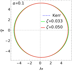
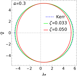
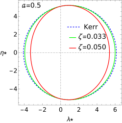
Figure 3: The dCS shadows as seen by a distant equatorial observer $\theta_{O}=\pi/2$ for different spin parameters $a=0.1,0.3,0.5$, as well as different values of $\zeta=0.033,0.050$. The curves are plotted with the help of equations $\lambda*$ and $\eta*$.

5.3 Images of dCS black hole with accretion disk

Accretion disks, essential elements situated in the equatorial plane of black holes, play a crucial role in the emission of observable light. These dynamic structures are characterized by a continuous flow of matter. The behavior of matter within the accretion disk is significantly influenced by its proximity to the black hole. To create these images, we use a thin accretion disk, as described in Ref. [1974ApJ…191..499P]. This model simplifies the analysis of accretion processes by assuming that the disk is geometrically thin compared to its radial extent. In addition, the disk is considered stationary and axisymmetric. These simplifications allow us to describe a two-dimensional disk using few important parameters such as the mass and spin of the black hole, the dimensionless coupling parameter of dCS, $\zeta$, the radius of the ISCO that determines the smallest stable orbits of massive particles, the geometrical thickness of the disk in geometric units, the angle (in radians) between spin axis and disk surface, and the position of observer angle that we fix to $\theta_{O}=\pi/2$. In Figure 4, we present thin accretion disks surrounding both a Kerr ($a=0.1$) and a dCS ($a=0.1$, $\zeta=0.024,0.057$) generated numerically, with superimposed images of null geodesics (dotted lines) of a photon sphere, obtained using the Hamilton-Jacobi formalism. At the given resolution of the figure (1000 × 1000 pixels), the images of Kerr and dCS for $\zeta=0.024$ black holes are indistinguishable from the naked eye. Any disparities between the two images are of the order of pixel size. On the other hand, for $\zeta=0.057$, differences emerge between the analytically generated geodesic and the numerically generated background. Considering our approximation scheme, it is important to note that the precision of the analytic solutions decreases for higher values of $\zeta$.

These images were generated using the Gyoto code, an open-source ray tracing tool [Vincent_2011]. Gyoto operates by numerically integrating null geodesic equations in a backward fashion, commencing from the observer’s screen. This technique allows for the computation of visual representations of the accretion disk around the black hole .

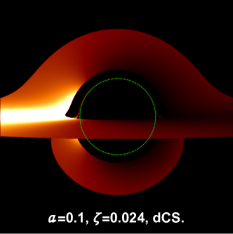
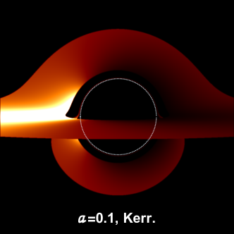
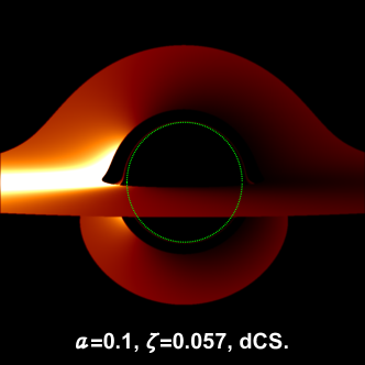
Figure 4: Left: Kerr black hole shadows with $a=0.1$ (white dotted line), superposed on the image of a geometrically thin accretion disk for the Kerr metric with $a=0.1$ in the equatorial plane $\pi/2$. Right: The shadow curve of the dCS with $a=0.1$ (green dotted line) superposed on the image of a geometrically thin accretion disk for the dCS metric with $a=0.1$ (images produced by Gyoto [52]).

5.4 Observables for the shadow

In this section, we analyze quantitatively the difference between the shadow of rotating black holes in dCS theory and in GR. To this end, we compute the shadow radius $R_{s}$ and the distortion parameter $\delta_{s}$. These observables enable us to perform a precise exploration of the deviations with respect to the Kerr shadow. Our methodology is based on the well-established framework provided in Refs. [Hioki_2009,Wei_2019]. The shadow radius $R_{s}$, defined in Ref. [Hioki_2009] as

$$R_{s}=\frac{\left(\lambda*_{t}-\lambda*_{r}\right)^{2}+\eta*^{2}_{t}}{2\left|\lambda*_{r}-\lambda*_{t}\right|},$$ (62)

characterizes the radius of a reference circle. The quantities in the definition above correspond to the points $T$ and $R$ shown in Fig. 5, whose coordinates are $(\lambda*_{t},\eta*_{t})$ and $(\lambda*_{r},0)$, respectively.

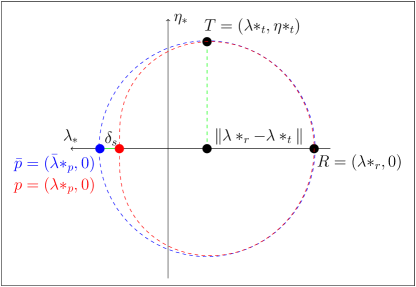
Figure 5: The observable $\delta s$ quantifies the extent to which the actual shadow deviates from the reference circle, where $(\bar{\lambda}*_{p},0)$ and $(\lambda*_{p},0)$ represent points where the reference circle and the shadow contour intersect the horizontal axis, positioned on the opposite side of $(\lambda*_{r},0)$.

On the other hand, the distortion parameter $\delta_{s}$ quantifies the extent to which the actual shadow deviates from the reference circle and is defined by

$$\delta_{s}=\frac{\left|\bar{\lambda}*_{p}-\lambda*_{p}\right|}{R_{s}},$$ (63)

where $(\bar{\lambda}*_{p},0)$ and $(\lambda*_{p},0)$ represent points where the reference circle and the shadow contour intersect the horizontal axis, positioned on the opposite side of $(\lambda*_{r},0)$, as shown in Fig. 5. The observables $R_{s}$ and $\delta_{s}$ as functions of the dCS dimensionless coupling parameter $\zeta$ are shown in Fig. 6.

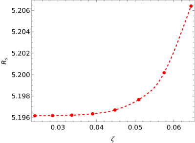
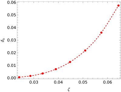
Figure 6: The observables $R_{s}$ and $\delta_{s}$ as functions of the dCS coupling parameter $\zeta$, corresponding to the shadow of a black hole positioned at the origin of coordinates and in the equatorial plane, with spin parameter $a=0.1$. As $\zeta$ increases, the shadow becomes more distorted.

To reach precise and physically consistent conclusions, we employ the relative difference $D_{s}$ taking a Kerr black hole as a reference,

$$D_{s}=\left|\frac{\lambda*_{r}-\lambda*_{rcs}}{\frac{\lambda*_{r}+\lambda*_{rcs}}{2}}\right|.$$ (64)

As shown in the previous section, the coordinate $\lambda*_{r}$ is significantly affected by the value of the CS coupling parameter. For this reason, $D_{s}$ is a good measurement of the deformations due to dCS. The estimation of this observable is reported in Figure 7. In the same figure, we include the distortion allowed by the uncertainty in the shadow radius of $SgA^{*}$, represented with a square marker. This distortion is obtained from Eq. (64) by associating $\lambda*_{r}$ to the central value of the $SgA^{*}$ shadow’s radius and $\lambda*_{rcs}$ to the maximum value allowed by the observational uncertainty. Large values of $\zeta$ are ruled out because they lead to distortions that are incompatible with this observation. This shows that the relative difference $D_{s}$ serves as a means of quantifying the deviations within the shadow. These deviations are directly attributed to variations in the coupling constants $\alpha$ and $\beta$ associated with the scalar field in the context of dCS modified gravity.

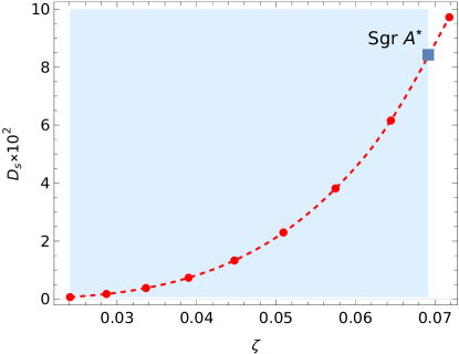
Figure 7: The relative difference $D_{s}$ with respect to a Kerr black hole measured from $(\lambda*_{r},0)$ as functions of the dCS coupling parameter $\zeta$, corresponding to the shadow of a black hole positioned at the origin of coordinates in the equatorial plane $\vartheta_{O}=\pi/2$ and the spin parameter $a=0.1$.

6 Discussion

In our investigation, we explore the behavior of null geodesics around a slowly rotating black hole within the framework of dCS modified gravity. This study specifically delves into scenarios characterized by a small coupling constant. A determining observation in our analysis is the separability of the Hamilton-Jacobi equation. However, it is crucial to acknowledge that for certain black hole solutions the Hamilton-Jacobi equation does not readily permit variable separation. To address this limitation, we use an approach based on the hierarchy of expansion orders of inverse powers of the radial coordinate, which facilitates the identification of the most significant modifications to the geodesic equations, thus allowing us to systematically neglect some terms from the equations of motion.

From these equations we find that the shape of a black hole shadow in dCS modified gravity depends primarily on the parameters $m$, $a$ and $\zeta$. The mass parameter is relevant to determine the size of the shadow, while $a$ and $\zeta$ are responsible for the deviation from the perfect circularity. This implies that the appearance of a shadow becomes a distinguishing factor between Kerr geometry and its dCS modification.

In this alternative theoretical framework, with a fixed rotation parameter $a$, the shadow consistently appears larger and more distorted than predicted by GR. The distortion increases progressively with higher values of $\zeta$, mainly due to the substantial influence of the dCS term.

These predictions can be validated in the future by cross-referencing with observations from the EHT, potentially substantiating or refuting theories associated with modified gravity. By scrutinizing the shadows cast by black holes, we stand on the brink of refining our understanding of the Universe, gradually reducing the range of possible models that can explain our astronomical observations.

7 Acknowledgments

This work was partially supported by CONAHCyT grants 932448 and DCF-320821.

References

- [1] C. M. Will, Living Reviews in Relativity 17 (Jun 2014).
- [2] S. Perlmutter, G. Aldering, G. Goldhaber, R. A. Knop, P. Nugent, P. G. Castro, S. Deustua, S. Fabbro, A. Goobar, D. E. Groom, I. M. Hook, A. G. Kim, M. Y. Kim, J. C. Lee, N. J. Nunes, R. Pain, C. R. Pennypacker, R. Quimby, C. Lidman, R. S. Ellis, M. Irwin, R. G. McMahon, P. Ruiz-Lapuente, N. Walton, B. Schaefer, B. J. Boyle, A. V. Filippenko, T. Matheson, A. S. Fruchter, N. Panagia, H. J. M. Newberg, W. J. Couch and T. S. C. Project, The Astrophysical Journal 517 (Jun 1999) 565.
- [3] A. G. Riess, A. V. Filippenko, P. Challis, A. Clocchiatti, A. Diercks, P. M. Garnavich, R. L. Gilliland, C. J. Hogan, S. Jha, R. P. Kirshner, B. Leibundgut, M. M. Phillips, D. Reiss, B. P. Schmidt, R. A. Schommer, R. C. Smith, J. Spyromilio, C. Stubbs, N. B. Suntzeff and J. Tonry, The Astronomical Journal 116 (Sep 1998) 1009.
- [4] Y. Sofue and V. Rubin, Annual Review of Astronomy and Astrophysics 39 (Sep 2001) 137.
- [5] A. Stepanian, S. Khlghatyan and V. G. Gurzadyan, The European Physical Journal Plus 136 (January 2021).
- [6] D. Ayzenberg and N. Yunes, Classical and Quantum Gravity 35 (November 2018) 235002.
- [7] X.-M. Kuang, Z.-Y. Tang, B. Wang and A. Wang, Phys. Rev. D 106 (Sep 2022) 064012.
- [8] G. Antoniou, A. Papageorgiou and P. Kanti, Universe 9 (March 2023) 147.
- [9] T. E. H. T. Collaboration, The Astrophysical Journal Letters 875 (Apr 2019) L1.
- [10] Event Horizon Telescope Collaboration, ”ApJL” 930 (May 2022) L12.
- [11] N. Yunes and L. C. Stein, Physical Review D 83 (May 2011).
- [12] R. Jackiw and S.-Y. Pi, Physical Review D 68 (Nov 2003).
- [13] A. Lue, L. Wang and M. Kamionkowski, Physical Review Letters 83 (Aug 1999) 1506.
- [14] M. Li, J.-Q. Xia, H. Li and X. Zhang, Physics Letters B 651 (Aug 2007) 357.
- [15] S. H. S. Alexander and S. J. Gates, Journal of Cosmology and Astroparticle Physics 2006 (Jun 2006) 018.
- [16] S. H. S. Alexander, M. E. Peskin and M. M. Sheikh-Jabbari, Physical Review Letters 96 (Feb 2006).
- [17] N. Yunes, D. Psaltis, F. Özel and A. Loeb, Physical Review D 81 (Mar 2010).
- [18] P. Wagle, N. Yunes and H. O. Silva, Physical Review D 105 (Jun 2022).
- [19] K. Yagi, N. Yunes and T. Tanaka, Physical Review D 86 (Aug 2012).
- [20] D. Grumiller, R. Mann and R. McNees, Physical Review D 78 (Oct 2008).
- [21] J. W. York, Phys. Rev. Lett. 28 (Apr 1972) 1082.
- [22] J. Erdmenger, B. Heß, I. Matthaiakakis and R. Meyer, Universal gibbons-hawking-york term for theories with curvature, torsion and non-metricity (2022).
- [23] M. Kimura, Physical Review D 98 (Jul 2018).
- [24] N. Yunes and F. Pretorius, Physical Review D 79 (Apr 2009).
- [25] L. Amarilla, E. F. Eiroa and G. Giribet, Phys. Rev. D 81 (Jun 2010) 124045.
- [26] S. Alexander and N. Yunes, Physics Reports 480 (August 2009) 1–55.
- [27] R. P. Kerr, Phys. Rev. Lett. 11 (Sep 1963) 237.
- [28] L. Ryder (2009).
- [29] S. M. Carroll, Lecture notes on general relativity (1997).
- [30] D. C. Wilkins, Phys. Rev. D 5 (Feb 1972) 814.
- [31] M. Fathi, M. Olivares and J. Villanueva, The European Physical Journal Plus 138 (12 2022).
- [32] E. Teo, General Relativity and Gravitation 53 (Jan 2021).
- [33] V. Perlick and O. Y. Tsupko, Physical Review D 95 (May 2017).
- [34] S. Chandrasekhar, The mathematical theory of black holes 1985.
- [35] V. Perlick and O. Y. Tsupko, Physics Reports 947 (Feb 2022) 1.
- [36] J. P. Luminet, AA 75 (May 1979) 228.
- [37] J. L. Synge, Monthly Notices of the Royal Astronomical Society 131 (02 1966) 463, https://academic.oup.com/mnras/article-pdf/131/3/463/8076763/mnras131-0463.pdf.
- [38] J. M. Bardeen, Proceedings, Ecole d’Eté de Physique Théorique: Les Astres Occlus : Les Houches, France, August, 1972, 215-240 (1973) 215.
- [39] Y. Brihaye and E. Radu, Physics Letters B 764 (Jan 2017) 300.
- [40] A. Grenzebach, The shadow of black holes : an analytic description (Springer, Switzerland, 2016).
- [41] A. Grenzebach, V. Perlick and C. Lämmerzahl, Physical Review D 89 (Jun 2014).
- [42] A. Grenzebach, V. Perlick and C. Lämmerzahl, International Journal of Modern Physics D 24 (Jul 2015) 1542024.
- [43] T. Johannsen and D. Psaltis, The Astrophysical Journal 718 (Jun 2010) 446.
- [44] S. Vázquez and E. Esteban, Il Nuovo Cimento B 119 (Dec 2004) 489–519.
- [45] D. Grumiller and N. Yunes, Physical Review D 77 (Feb 2008).
- [46] S. Alexander and N. Yunes, Physics Reports 480 (Aug 2009) 1.
- [47] K. Konno, T. Matsuyama and S. Tanda, Physical Review D 76 (Jul 2007).
- [48] K. Konno, T. Matsuyama and S. Tanda, Progress of Theoretical Physics 122 (Aug 2009) 561.
- [49] Y. Ali-Haïmoud and Y. Chen, Physical Review D 84 (Dec 2011).
- [50] C. F. Sopuerta and N. Yunes, Physical Review D 80 (September 2009).
- [51] D. N. Page and K. S. Thorne, ApJ 191 (July 1974) 499.
- [52] F. H. Vincent, T. Paumard, E. Gourgoulhon and G. Perrin, Classical and Quantum Gravity 28 (Oct 2011) 225011.
- [53] K. Hioki and K. ichi Maeda, Physical Review D 80 (Jul 2009).
- [54] S.-W. Wei, Y.-X. Liu and R. B. Mann, Physical Review D 99 (Feb 2019).