Rotating fermion-boson stars

Abstract

Rotating fermion-boson stars are hypothetical celestial objects that consist of both fermionic and bosonic matter interacting exclusively through gravity. Bosonic fields are believed to arise in certain models of particle physics describing dark matter and could accumulate within neutron stars, modifying some of their properties and gravitational wave emission. Fermion-boson stars have been extensively studied in the static non-rotating case, exploring their combined stability and their gravitational radiation in binary mergers. However, stationary rotating configurations were yet to be found and investigated. The presence of a bosonic component could impact the development of the bar-mode instability in differentially rotating neutron stars. Therefore, the study of rotating fermion-boson stars has important implications for astrophysics, as they could provide a new avenue for the detection of gravitational waves. In addition, these objects may shed light on the behavior of matter under extreme conditions, such as those found in the cores of neutron stars, and explain any tension in the determination of the dense-matter equation of state from multi-messenger observations. In this work we study a new consistent method of constructing uniformly rotating fermion-boson stars and we analyse some of their main properties. These objects might offer alternative explanations for current observations populating the lower black-hole mass gap, as the $2.6M_{\odot}$ compact object involved in GW190814.

I Introduction

Neutron stars (NS) are a focal point of numerous studies due to their unique and remarkable properties. They present an exceptional opportunity to examine various areas of physics, including nuclear physics, gravitational physics, and astrophysics. Both binary systems and isolated neutron stars are being scrutinized in depth to test General Relativity and different theories of gravity under strong field conditions. Furthermore, with regard to nuclear matter research, recent findings by the Neutron Star Interior Composition Explorer (NICER) have substantially strengthened constraints on the Equation of State (EOS), and have also furnished highly precise and reliable measurements for the mass and equatorial radius of various millisecond pulsars Ozel et al. (2016); Miller et al. (2019a).

Binary NS systems are considered one of the most promising sources of gravitational waves that can be detected by the advanced LIGO, advanced VIRGO, and KAGRA observatories Akutsu et al. (2019); Abbott et al. (2022). Moreover, the combined use of different types of observations has significantly improved our understanding of compact objects and other astrophysical phenomena. We are entering the era of multi-messenger astronomy, where the simultaneous detection of signals from multiple messengers (electromagnetic and gravitational waves, neutrinos) results in more accurate and precise measurements of physical quantities associated with NSs Raaijmakers et al. (2020).

Many NS properties are of significant interest, including quadrupole moments, spin angular velocity, which is directly proportional to the moment of inertia, and their tidal and rotational deformability, often represented by the Love numbers Hinderer (2008); Postnikov et al. (2010). In August 2017, the first gravitational wave (GW) signal from the merger of a compact low-mass NS binary was observed by the LIGO-Virgo detector network Abbott et al. (2017a), which was followed by an electromagnetic counterpart Abbott et al. (2017b). Similar systems have since been detected and are currently under investigation Abbott et al. (2020a). Future new detections of gravitational waveforms emitted by these systems could be used to constrain the parameters of the equation of state of NSs and learn more about their internal composition Abbott et al. (2018); Raithel (2019).

On the other hand, theoretical exotic compact objects could also populated the Universe. One of the simplest examples are boson stars (BSs), compact horizonless, regular solutions of an ultralight bosonic field theory minimally coupled to gravity, which involves a complex scalar field $\Phi$. However, solutions for massive vector fields (aka Proca stars or vector boson stars) have also been obtained, both with and without rotation (for a thorough understanding on BSs, we refer the interested reader to Liebling and Palenzuela (2012); Lai (2004); Schunck and Mielke (2003); Brito et al. (2016); Herdeiro et al. (2019); Sanchis-Gual et al. (2019)). The concept of BSs dates back to the proposal of geons by Wheeler Wheeler (1955) and the introduction of the original spherical scalar BSs by Kaup Kaup (1968), Ruffini, Bonazzola, and Pacini RUFFINI and BONAZZOLA (1969); Bonazzola and Pacini (1966). The properties of BSs are primarily determined by the potential that encodes the self-interaction of the complex scalar field and varies with the Lagrangian form. Different potentials can be used to model various astrophysical objects, such as black-hole mimickers with features resembling those of NSs or even black holes Guzmán and Rueda-Becerril (2009); Olivares et al. (2020); Herdeiro et al. (2021); Pitz and Schaffner-Bielich (2023); Rosa et al. (2022); Rosa and Rubiera-Garcia (2022); Rosa et al. (2023, 2024); Sengo et al. (2024). Additionally, BSs and ultralight bosonic fields are considered promising candidates to account for (part of) the dark matter present in galaxy halos Schunck (1998).

There are several unconventional extensions of BSs, which involve more generalized models of gravity, such as Palatini gravity Masó-Ferrando et al. (2021), Einstein-Gauss-Bonnet theory, scalar-tensor models Torres (1997), or the semi-classical gravity framework Alcubierre et al. (2022). Apart from these generalizations, recently considerable effort has been invested into the exploration of more exotic BS models, including multi-state BSs Urena-Lopez and Bernal (2010), $\ell$-BSs Alcubierre et al. (2018), multi-field multi-frequency BSs Sanchis-Gual et al. (2021), Proca-Higgs stars Herdeiro et al. (2023), scalar-vector stars, also called Scalaroca stars Pombo et al. (2023), and $\ell$-Proca stars Lazarte and Alcubierre (2024).

In recent years there has been a surge of interest in the search of additional scalar or vector degrees of freedom. One reason for this was the discovery of the fundamental scalar Higgs boson at CERN Aad et al. (2012); Chatrchyan et al. (2012), which has provided a theoretical motivation for the existence of additional scalar fields beyond the Standard Model, such as the axion Weinberg (1978); Wilczek (1978); Guo et al. (2023) or other ultralight scalar or vector bosons Arvanitaki et al. (2010); Freitas et al. (2021), which have been proposed as potential dark matter particles Khlopov (2024). The potential detection of new fundamental vector fields through future observations with LISA is a highly motivating factor for the continued study of these types of objects Fell et al. (2023).

As for NSs, GW astronomy presents a new avenue for the exploration of exotic compact objects, which includes BSs. In this auspicious context, an exceptional GW signal was detected in 2020 by advanced LIGO-Virgo, which could potentially be interpreted as the result of a head-on collision of two Proca stars Bustillo et al. (2021) (see also Calderon Bustillo et al. (2023)). Furthermore, current research efforts are also focused on studying the merger dynamics of BS binaries Palenzuela et al. (2017); Bezares et al. (2019); Sanchis-Gual et al. (2022); Bezares et al. (2022); Siemonsen and East (2023); Atteneder et al. (2024).

If a primordial gas could give rise to bosonic configurations, it is plausible that fermions could also be present during condensation. This suggests the possibility of mixed configurations, consisting of both bosons and fermions. While the original configurations might have been mainly composed of either bosons or fermions, they could also have captured additional fermions and bosons through accretion.

Thus, it is an intriguing theoretical question to explore the properties of these macroscopic composites, which are known as fermion-boson stars in the literature Henriques et al. (1990a). The initial research on the topic was conducted at the end of $1980s$ Henriques et al. (1989, 1990b); Valdez-Alvarado et al. (2013a). Other generalizations have also been studied, like charged fermion-boson stars Kain (2021) and fermion-Proca stars Jockel and Sagunski (2024). Numerical simulations have been performed to study their stability and the possible mechanisms through which they could form Valdez-Alvarado et al. (2013b); Di Giovanni et al. (2020a, 2021); Nyhan and Kain (2022); Di Giovanni et al. (2022a). It is worth mentioning that recent studies have applied perturbative methods over the static background, obtaining the tidal deformability for mixed stars Diedrichs et al. (2023).

From the astrophysical point of view, non-zero angular momentum stars are important, and the slowly rotating limit was studied in de Sousa and Silveira (2001). Recent measurements have identified the most rapidly rotating and massive NS in our galaxy to date. Designated as PSR J0952-0607, this NS was initially discovered by Bassa et al. (2017) in 2017. It exhibits an exceptionally short rotational period of $1.41$ milliseconds. Further investigations by Romani et al. (2022) have revealed that the NS possesses a significantly high mass, estimated to be $M=2.35\pm 0.17M_{\odot}$. Additionally, the secondary component of the GW event GW190814 could also be a massive NS with $M=2.6M_{\odot}$ Abbott et al. (2020b). These findings provide substantial support for the theory that mixed stars could be plausible explanations for such astrophysical phenomena Lee et al. (2021); Das et al. (2021a); Di Giovanni et al. (2022b); Valdez-Alvarado et al. (2024).

In this work we obtain stationary solutions of the Einstein-Euler-Klein-Gordon system, where fermionic and bosonic matter are coupled only through gravity, both have angular momentum and form a spinning mixed fermion-boson star.

In section II, we establish the theoretical framework, delineating each component and the system as a whole to elucidate the types of objects presented in this manuscript. Section III is devoted to the numerical treatment and the development of the algorithm employed for solving the systems. The main global properties of our solutions are obtained in section IV, whereas a thorough analysis of the solutions is presented in section V. The section VI delves into how these types of objects integrate into the GW paradigm, providing some insights into their significance and implications, while section VII is devoted to some final remarks and conclusions. An appendix appendix A with some more equations of interest closes the manuscript. Through this work, we adopt $G=c=1$ units.

II Formalism

We will first introduce the framework to obtain numerical solutions of NSs and BSs, since fermionic and bosonic matter describing them behave differently. Besides, the numerical methods for solving each type of star separately are significantly different. In this section, we describe the theoretical set-up and numerical methods to build stationary NSs and BSs separately.

II.1 Neutron Stars and RNS

We can model uniformly rotating NSs described as a perfect fluid assuming a stationary, axisymmetric space-time. The circular velocity $u^{\alpha}$ can be written in terms of two Killing vectors $t^{\alpha}$ and $\psi^{\alpha}$, being,

$$u^{\alpha}=u^{t}(t^{\alpha}+\Omega\psi^{\alpha}),$$ (1)

where,

$$u^{t}\coloneqq\left[g_{\alpha\beta}(t^{\alpha}+\Omega\psi^{\alpha})(t^{\beta}+\Omega\psi^{\beta})\right]^{1/2},$$ (2)

is the $t$ component of $u^{\alpha}$. In the natural coordinates of $t$ and $\psi$, the angular velocity of the fluid as seen by an observer at rest at infinity can be expressed as follows,

$$\Omega\equiv\frac{u^{\psi}}{u^{t}}=\frac{d\psi}{dt}.$$ (3)

We will have uniform rotation if and only if $\Omega=\text{constant}$. The metric $g_{\alpha\beta}$ for the system can be written as

$$\begin{split}ds^{2}=&-e^{\gamma+\rho}dt^{2}+e^{\gamma-\rho}r^{2}\sin^{2}{\theta}\left(d\psi-\omega dt\right)^{2}\\ &+e^{2\alpha}\left(dr^{2}+r^{2}d\theta^{2}\right),\end{split}$$ (4)

where $\gamma,\rho,\alpha$ and $\omega$ are functions of $r$ and $\theta$ Friedman and Stergioulas (2013). The stress-energy tensor that describes our matter source is given by

$$T^{\alpha\beta}=\left(\rho_{0}+\rho_{i}+P\right)u^{\alpha}u^{\beta}+Pg^{\alpha\beta},$$ (5)

where $\rho_{0}$ is the rest-energy density, $\rho_{i}$ is the internal energy density and $P$ is the pressure.

We solve the Einstein field equations

$$G_{\alpha\beta}=R_{\alpha\beta}-\frac{1}{2}Rg_{\alpha\beta}=8\pi T_{\alpha\beta},$$ (6)

coupled to the Euler equations in order to obtain solutions of rotating NSs. To do this we will employ the RNS code Stergioulas and Friedman (1995), which is based on the Komatsu, Eriguchi, and Hachisu method, also known as the Hachisu self-consistent field (HSCF) Komatsu et al. (1989). This method makes use of a Green’s function approach, in which the Einstein field equations are manipulated to isolate terms for which the flat-space Green’s function is known. The remaining terms (referred to as the sources) are moved to the right-hand side. The metric functions are then determined at each iteration through an integral involving the sources (including the stress-energy tensor and other elements) and Green’s functions. This approach combines different aspects of spectral methods and finite difference techniques, and was modified by Teukolsky, Cook, and Shapiro Cook et al. (1992).

Taking the above into account, the Einstein field equations will be presented as second-order partial derivative operators over some combinations of the metric potentials, equated to the source terms,

$$\Delta\left[\rho e^{\gamma/2}\right]=S_{\rho}(r,\mu),$$ (7)

$$\left(\Delta+\frac{1}{r}\partial_{r}-\frac{\mu}{r^{2}}\partial_{\mu}\right)\left[\gamma e^{\gamma/2}\right]=S_{\gamma}(r,\mu),$$ (8)

$$\left(\Delta+\frac{2}{r}\partial_{r}-\frac{2\mu}{r^{2}}\partial_{\mu}\right)\left[\omega e^{(\gamma-\rho)/2}\right]=S_{\omega}(r,\mu),$$ (9)

with $\Delta$ the flat-space, spherical coordinate Laplacian, $\mu=\cos\theta$, and $S_{\rho}$, $S_{\gamma}$, $S_{\omega}$ are the mentioned sources, shown in the Appendix A. The fourth field equation determines $\alpha$ and it is not separable in this way. The four field equations together with the hydrostatic equilibrium one,

$$dP-\left(\rho_{0}+\rho_{i}+P\right)\left[d\ln u^{t}+u^{t}u_{\phi}d\Omega\right],$$ (10)

and a given EOS close the problem. The behavior of the fermionic matter in this work is assumed to follow a polytropic law for simplicity,

$$P=K\rho_{t}^{1+1/n},$$ (11)

where $\Gamma=1+1/n$ is the adiabatic index and $K$ is the polytropic constant, which will determine our scale all over the work. Further, $\rho_{t}=\rho_{0}+\rho_{i}$ is the total energy density. Since $K^{n/2}$ has units of length, we can use it to redefine dimensionless quantities and fix the scale of our system.

We will first define the zero angular momentum observer (ZAMO) velocity,

$$v=(\Omega-\omega)r\sin\theta e^{-\rho},$$ (12)

which will be useful in what follows.

The metric functions are numerically determined by integrating the sources defined by eqs. 7, 8 and 9, where we use the method of the Green functions for the radial part, and the corresponding polynomials for the angular dependence. This is the RNS philosophy.

II.2 Boson stars

The complex scalar field dynamics are described by the Lagrangian,

$$\mathcal{L}_{\Phi}=-\frac{1}{2}\left[g^{\alpha\beta}\nabla_{\alpha}\Phi^{*}\nabla_{\beta}\Phi+V\left(|\Phi|^{2}\right)\right],$$ (13)

where $V\left(|\Phi|^{2}\right)$ is a potential that depends only on the absolute value of the scalar field, respecting the global $U(1)$ invariance of the model.

Through a minimal coupling to gravity, the above enters the action in the following manner Liebling and Palenzuela (2012),

$$\mathcal{S}=\int\left(\frac{1}{16\pi G}R+\mathcal{L}_{\Phi}\right)\sqrt{-g}d^{4}x.$$ (14)

This equation, called the Einstein-Klein-Gordon (EKG) action, describes the behavior of a massive complex scalar field $\Phi$ coupled to Einstein’s gravity. In the former equation, $g$ is the metric determinant, and $R$ is the Ricci scalar.

Varying the action (14) yields the EKG equations,

$$\begin{split}&R_{\alpha\beta}-\frac{1}{2}Rg_{\alpha\beta}=8\pi T_{\alpha\beta},\\ &g^{\alpha\beta}\nabla_{\alpha}\nabla_{\beta}\Phi=\frac{dV}{d|\Phi|^{2}}\Phi,\end{split}$$ (15)

where $T_{\alpha\beta}$ is now the canonical stress-energy tensor of the scalar field,

$$T_{\alpha\beta}=2\nabla_{(\alpha}\Phi^{*}\nabla_{\beta)}\Phi-2g_{\alpha\beta}\left[g^{\mu\nu}\nabla_{(\mu}\Phi^{*}\nabla_{\nu)}\Phi+V\left(|\Phi|^{2}\right)\right]],$$ (16)

and $R_{\alpha\beta}$ is the Ricci tensor. Equilibrium solutions are obtained assuming an axisymmetric coordinate system as in eq. 4 and the following ansatz for the field, as in Herdeiro and Radu (2015); Ryan (1997a),

$$\Phi(t,r,\theta,\psi)=\phi(r,\theta)e^{-i(wt+\eta\psi)}.$$ (17)

The angular frequency of the field is $w\in\mathbb{R}$ and $\eta\in\mathbb{Z}$ is the harmonic index, also called the winding number and the complex scalar field modulus is $|\Phi(t,r,\theta,\psi)|=\phi(r,\theta)$.

II.3 Mixed stars and rotating fermion-boson stars

Several studies have been conducted on the static case of mixed fermion-boson configurations Di Giovanni et al. (2020a); Nyhan and Kain (2022); Di Giovanni et al. (2022a, 2021); Valdez-Alvarado et al. (2013a); Kain (2021). However, since rotation is a ubiquitous phenomenon in astrophysics, we aimed to develop a framework for solving the Einstein equations for mixed rotating stars, which are more closely aligned with plausible astrophysical scenarios.

In this initial approach, we have developed a code that can solve the Einstein equations for an axisymmetric spacetime with a matter content of fermions and bosons that are coupled solely by gravity,

$$R_{\alpha\beta}-\frac{1}{2}Rg_{\alpha\beta}=G_{\alpha\beta}=8\pi(T^{f}_{\alpha\beta}+T^{b}_{\alpha\beta}).$$ (18)

The metric ansatz is precisely eq. 4. The stress-energy tensor for the fermionic matter, i.e. the neutron star component, is represented by $T_{\alpha\beta}^{f}$ and it is exactly eq. 5, while $T_{\alpha\beta}^{b}$ represents the stress-energy tensor for the bosonic matter given by eq. 16. The Einstein equations can be reformulated in terms of the aforementioned differential operators and sources,

$$\begin{split}&\Delta\left[\rho e^{\gamma/2}\right]=S_{\rho}^{T}(r,\mu),\\ &\left(\Delta+\frac{1}{r}\partial_{r}-\frac{\mu}{r^{2}}\partial_{\mu}\right)\left[\gamma e^{\gamma/2}\right]=S_{\gamma}^{T}(r,\mu),\\ &\left(\Delta+\frac{2}{r}\partial_{r}-\frac{2\mu}{r^{2}}\partial_{\mu}\right)\left[\omega e^{(\gamma-\rho)/2}\right]=S_{\omega}^{T}(r,\mu),\end{split}$$ (19)

The sources corresponding to the bosonic part, are obtained using the high coupling-constant approximation, following Ryan (1997b); Vaglio et al. (2022) where such approach is used and explained in what follows. It is important to notice that when computing the source terms for the mixed star, we have contributions from the fermionic and bosonic matter, but also some curvature contributions which cannot be computed twice, i.e with a total stress-energy tensor given by $T^{T}_{\alpha\beta}=(T^{f}_{\alpha\beta}+T^{b}_{\alpha\beta})$, the full sources $S_{i}^{T}\neq S_{i}^{f}+S_{i}^{b}$.

In the above-mentioned framework, we have the following potential:

$$V(|\Phi|)=\mu_{b}^{2}|\Phi|^{2}+\frac{1}{2}\lambda|\Phi|^{4},$$ (20)

where $\mu_{b}$ is the boson scalar field mass (not to be confused with $\mu=\cos\theta$) and $\lambda$ the coupling or self-interacting constant. In the high-coupling approximation, although the ansatz for the field is eq. 17, we marginalize the bosonic tail and assume that the scalar field in the outer region is $|\Phi|=0$, while, in the inner part,

$$|\Phi|^{2}={\rm{max}}\left[0,\frac{1}{\lambda}\left(\frac{(w-\eta\omega)^{2}}{e^{\gamma+\rho}}-\frac{e^{\rho-\gamma}\eta^{2}}{r^{2}\sin^{2}\theta}-\mu_{b}^{2}\right)\right].$$ (21)

Moreover, the stress-energy tensor for the bosonic matter reduces to that of an analogous perfect fluid describing the interior of the star, while the exponential tail region identified as the outer part is neglected under this approximation,

$$T_{\mu\nu}^{b}=(\rho_{BS}+P_{BS})\hat{u}_{\mu}\hat{u}_{\nu}+P_{BS}g_{\mu\nu}.$$ (22)

The pressure and energy density are given by

$$P_{BS}=\frac{1}{4}\lambda|\Phi|^{4},\hskip 14.22636pt\rho_{BS}=\mu_{b}^{2}|\Phi|^{2}+\frac{3}{4}\lambda|\Phi|^{4},$$ (23)

and the four-velocity,

$$(\hat{u}_{t},\hat{u}_{r},\hat{u}_{\theta},\hat{u}_{\psi})=\frac{(-w,0,0,\eta)}{(\lambda|\Phi|^{2}+\mu_{b}^{2})^{\frac{1}{2}}}.$$ (24)

So the proper velocity of the zero angular momentum observer is given by,

$$\bar{v}=\frac{\eta}{(w-\eta\omega)}\frac{e^{\rho}}{r\sin\theta}.$$ (25)

As under this approximation the stress-energy tensor can be re-expressed in a perfect-fluid-like form, we obtain the source equations analogously to the NS case. We also have defined the energy density and pressure induced by the bosonic part, therefore the equations for the mixed stars will be similar to the NS ones, but with additional bosonic matter terms.

The corresponding sources are:

$$\begin{split}&S_{\rho}^{T}(r,\mu)=e^{\gamma/2}\left[8\pi e^{2\alpha}\left\{\left(\rho_{0}+\rho_{i}+P\right)\frac{1+v^{2}}{1-v^{2}}+\left(\rho_{BS}+P_{BS}\right)\frac{1+\bar{v}^{2}}{1-\bar{v}^{2}}\right\}+r^{2}(1-\mu^{2})e^{-2\rho}\left(\omega_{,r}^{2}+\frac{(1-\mu^{2})}{r^{2}}\omega^{2}_{,\mu}\right)+\right.\\ &\left.\frac{1}{r}\gamma_{r}-\mu\gamma_{,\mu}+\frac{\rho}{2}\left\{16\pi e^{2\alpha}\left(P+P_{BS}\right)-\gamma_{,r}\left(\frac{1}{2}\gamma_{,r}+\frac{1}{r}\right)-\frac{1}{r^{2}}\gamma_{,\mu}\left(\frac{1-\mu^{2}}{2}\gamma_{,\mu}-\mu\right)\right\}\right],\end{split}$$ (26)

$$S_{\gamma}^{T}(r,\mu)=e^{\gamma/2}\left[16\pi e^{2\alpha}\left(P+P_{BS}\right)+\frac{\gamma}{2}\left\{16\pi e^{2\alpha}\left(P+P_{BS}\right)-\frac{1}{2}\gamma_{,r}^{2}-\frac{1-\mu^{2}}{2r^{2}}\gamma_{,\mu}^{2}\right\}\right],$$ (27)

$$\begin{split}&S_{\omega}^{T}(r,\mu)=e^{(\gamma-2\rho)/2}\left[-16\pi e^{2\alpha}\left[\frac{(\Omega-\omega)(\rho_{0}+\rho_{i}+P)}{1-v^{2}}+\frac{\bar{v}\left(\rho_{BS}+P_{BS}\right)}{(1-\bar{v}^{2})r\sin\theta}\right]+\right.\\ &\left.\omega\left\{-8\pi e^{2\alpha}\left[\frac{(1+v^{2})(\rho_{0}+\rho_{i})+2v^{2}P}{1-v^{2}}+\frac{(1+\bar{v}^{2})\rho_{BS}+2\bar{v}^{2}P}{1-\bar{v}^{2}}\right]-\frac{1}{r}\left(2\rho_{,r}+\frac{1}{2}\gamma_{,r}\right)+\frac{\mu}{r^{2}}\left(2\rho_{,\mu}+\frac{1}{2}\gamma_{,\mu}\right)+\right.\right.\\ &\left.\left.\frac{1}{4}(4\rho_{,r}^{2}-\gamma_{,r}^{2})+\frac{1-\mu^{2}}{4r^{2}}(4\rho_{,\mu}^{2}-\gamma_{,\mu}^{2})-r^{2}(1-\mu^{2})e^{-2\rho}\left[\omega_{,r}^{2}+\frac{(1-\mu^{2})}{r^{2}}\omega_{,\mu}^{2}\right]\right\}\right],\end{split}$$ (28)

$$\begin{split}&\alpha^{T}_{,\mu}=-\frac{1}{2}\left(\rho_{,\mu}+\gamma_{,\mu}\right)-\left\{\left(1-\mu^{2}\right)\left[1+r\gamma_{,r}\right]^{2}+\left[\mu-\left(1-\mu^{2}\right)\gamma_{,\mu}\right]^{2}\right\}^{-1}\left[\frac{1}{2}\left[r^{2}\left[\gamma_{,rr}+\gamma_{,r}^{2}\right]\right.\right.\\ &\left.-\left(1-\mu^{2}\right)\left(\gamma_{,\mu\mu}+\gamma_{,\mu}^{2}\right)\right]\left[-\mu+\left(1-\mu^{2}\right)\gamma_{,\mu}\right]+r\gamma_{,r}\left[\frac{1}{2}\mu+\mu r\gamma_{r}+\frac{1}{2}\left(1-\mu^{2}\right)\gamma_{,\mu}\right]+\\ &\left.+\frac{3}{2}\gamma_{,\mu}\left[-\mu^{2}+\mu(1-\mu^{2})\gamma_{,\mu}\right]-r\left(1-\mu^{2}\right)\left(\gamma_{,r\mu}+\gamma_{,r}\gamma_{,\mu}\right)\left(1+r\gamma_{,r}\right)-\frac{1}{4}\mu r^{2}\left(\rho_{,r}+\gamma_{,r}\right)^{2}-\frac{r}{2}\left(1-\mu^{2}\right)\left(\rho_{,r}+\gamma_{,r}\right)\left(\rho_{,\mu}+\gamma_{,\mu}\right)\right.\\ &\left.+\frac{1}{4}\mu\left(1-\mu^{2}\right)\left(\rho_{,\mu}+\gamma_{,\mu}\right)^{2}-\frac{r^{2}}{2}\left(1-\mu^{2}\right)\gamma_{,r}\left(\rho_{,r}+\gamma_{,r}\right)\left(\rho_{,\mu}+\gamma_{,\mu}\right)+\frac{1}{4}\left(1-\mu^{2}\right)\gamma_{,\mu}\left[r^{2}\left(\rho_{,r}+\gamma_{,r}\right)^{2}-\left(1-\mu^{2}\right)\left(\rho_{,\mu}+\gamma_{,\mu}\right)^{2}\right]\right.\\ &\left.+\left(1-\mu^{2}\right)e^{-2\rho}\left\{\frac{1}{4}r^{4}\mu\omega_{,r}^{2}+\frac{1}{2}r^{3}\left(1-\mu^{2}\right)\omega_{,r}\omega_{,\mu}-\frac{1}{4}r^{2}\mu\left(1-\mu^{2}\right)\omega_{,\mu}^{2}+\frac{1}{2}r^{4}\left(1-\mu^{2}\right)\gamma_{,r}\omega_{,r}\omega_{,\mu}\right.\right.\\ &\left.\left.-\frac{1}{4}r^{2}\left(1-\mu^{2}\right)\gamma_{,\mu}\left[r^{2}\omega_{,r}^{2}-\left(1-\mu^{2}\right)\omega_{,\mu}^{2}\right]\right\}\right],\end{split}$$ (29)

where the equation for $\alpha^{T}$ is formally the same than for the NS case, eq. 61.

III Numerical implementation

III.1 Internal scaling

Our approach consists in using the RNS as the base code, and implementing the Ryan-Vaglio approximation for the BSs as additional source terms in the usual NSs algorithm. The code had to be modified to include the bosonic matter part but our algorithm is essentially the same RNS code, making use of the HSCF method based on Green functions to solve our system of equations. The main problem we dealt with was the different rescaling for both types of objects. As shown in the RNS bibliography Cook et al. (1992), the whole code uses a map between the compactified coordinate $s$ and the full spherical radius $r$ through the equatorial coordinate radius $r_{e}$, following

$$r=r_{e}\left(\frac{s}{1-s}\right).$$ (30)

Thus, let us explicitly derive the differentiation rule for this variable change,

$$\begin{split}&\frac{dr}{ds}=r_{e}\frac{d}{ds}\left(\frac{s}{1-s}\right)=r_{e}\left(\frac{(1-s)-s(-1)}{(1-s)^{2}}\right)\\ &\rightarrow dr=\frac{r_{e}}{(1-s)^{2}}ds.\end{split}$$ (31)

For the NS case, it is straightforward to obtain $r_{e}$, since it is the coordinate radius at the star’s surface, but when dealing with BSs or mixed stars, in the static case, it is not clear how to define this quantity, as the bosonic matter decays exponentially to zero at infinity in a non-compact form. This parameter is important because the method uses this radius as a scaling parameter. For each star, we should have a different value of $r_{e}$. To solve this issue, we have implemented the following criterion: on one hand, in the pure BS case, the $r_{e}$ is defined by the radius at which $99\%$ of the scalar field energy density is enclosed by a sphere of that radius. On the other hand, when we have a mixed star as the initial guess we simply take the fermionic $r_{e}$. We have checked the consistency and stability of the method for various mixed and purely bosonic spherical static stars, used as initial guesses, by having close but different values for $r_{e}$. For those constrained boundary conditions for the spinning case, we obtain the same solutions. The calculations involving the initial guesses are described in Appendix A.

As mentioned before, the scaling for the problem is defined by the polytropic constant $K$, i.e, the NS part. From Cook et al. (1994) we have the following dimensionless re-definitions,

$$\begin{split}&\bar{r}\equiv K^{-n/2}r,\\ &\bar{t}\equiv K^{-n/2}t,\\ &\bar{\omega}\equiv K^{n/2}\omega,\\ &\bar{\Omega}\equiv K^{n/2}\Omega,\\ &\bar{\rho}_{0}\equiv K^{n}\rho_{0},\\ &\bar{\rho}_{i}\equiv K^{n}\rho_{i},\\ &\bar{P}\equiv K^{n}P.\end{split}$$ (32)

For the BS part, the scaling with the polytropic constant may seem less natural than using the boson mass $\mu_{b}$, but as it is easier to use same scaling to build mixed configurations, we will maintain both the self-interaction constant and the mass potential. The re-scaled and dimensionless BS parameters are given by

$$\begin{split}&\bar{w}\equiv K^{n/2}w,\\ &\bar{\eta}\equiv K^{-n}\eta,\\ &\bar{\mu_{b}}\equiv K^{-n/2}\mu_{b},\\ &\bar{\lambda}\equiv K^{-n}\lambda.\end{split}$$ (33)

This also leads to the usual constraint for the frequency defined by $\bar{w}\in[0,\bar{\mu_{b}}]$. It is important to note that, at the level of the code, we do an effective re-scaling by fixing $\mu_{b}$ to unity, but as this boson mass is also re-scaled by our choice of the natural parameter for the problem (the polytropic constant), we cannot just remove it from the code, and it will appear as $\bar{\mu_{b}}$.

Having the aforementioned re-scaling rule settled, the observable quantities obtained are also dimensionless, and the transformation law is defined by,

$$\begin{split}&\bar{M}=K^{-n/2}M,\\ &\bar{J}=K^{-n}J,\end{split}$$

with $M$ and $J$ the mass and the angular momentum of the star, respectively.

III.2 Initial guess, shooting method, and coordinate transformation

The initial conditions can be obtained through two different calculations, depending on the inputs given to the code and the configurations we wish to obtain. In one case, if we want to build mixed stars that have a larger fermionic component, which is the main case of study here, the code will choose the spherical NS as the initial guess. The procedure to take a spherically symmetric star as the spinning star initial guess is well explained in the RNS manual Stergioulas (1992). However, we will give a brief explanation of how to implement all possible cases of initial conditions. Both the previously mentioned case in which the initial condition is obtained from a scenario in which the fermionic matter dominates, as well as the case in which there is a mixed initial condition or with bosonic dominance. The mixed and purely bosonic scenario can be obtained with a single, general formalism with the only condition of making zero or non-zero the fermionic energy density at the origin for having pure BSs or mixed stars. The Tolman-Oppenheimer-Volkoff (TOV) equations are solved for the given polytropic parameters, with the line element for a static spherical object defined by

$$ds_{SNS}^{2}=-e^{2\nu(r)}dt^{2}+\frac{1}{1-\frac{2m(r)}{r}}dr^{2}+r^{2}d\Omega.$$ (34)

Thus, we have static NSs described by the following system of equations:

EOS: $$P=P(\rho)$$

Mass: $$\frac{dm(r)}{dr}=4\pi r^{2}\rho(r)$$

Radial Einstein: $$\frac{d\nu(r)}{dr}=\frac{(m(r)+4\pi r^{3}P(r))}{r(r-2m(r))}$$

TOV: $$\frac{dP(r)}{dr}=-\nu^{\prime}(r)(\rho(r)+P(r)).$$ (35)

The RNS and our extension use a Runge-Kutta method to integrate the former equations. Then, a subroutine interpolates the interior of the stars and matches them with the outer solution, determined by the isotropic Schwarzschild metric coordinates, while for the interior part, it recovers the quasi-isotropic metric. The initial guess for the metric eq. 4 results in the following isotropic coordinates

INT: $$ds^{2}=-e^{2\nu}dt^{2}+e^{2\lambda}(dr^{2}+r^{2}d\theta+r^{2}\sin^{2}\theta d\psi^{2})$$

$$\Rightarrow \gamma=\nu+\lambda,\hskip 5.69046pt\rho=\nu-\lambda,\hskip 5.69046pt\alpha=(\gamma-\rho)/2,\hskip 5.69046pt\omega=0$$

OUT: $$e^{(\gamma+\rho)/2}=[1-M_{s}/(2r)]/[1+M_{s}/(2r)],$$

$$\Rightarrow e^{(\gamma-\rho)/2}=e^{\alpha}=(1+M_{s}/(2r))^{2},\hskip 5.69046pt\omega=0.$$ (36)

Through the previous transformations, the initial guess calculation for the scenario where fermionic matter is dominant, is straightforward. In contrast, posing an initial guess for a mixed star or a purely bosonic star requires a slightly different approach. Specifically, the metric ansatz must be expressed in quasi-isotropic coordinates and the TOV system needs the corresponding modifications. Our chosen metric in these cases is the same as the one used in Di Giovanni et al. (2020a),

$$ds^{2}=-b^{2}dt^{2}+a^{2}dr^{2}+(r^{2}d\theta+r^{2}\sin^{2}\theta d\psi^{2})$$ (37)

The scalar field ansatz in spherical symmetry is now

$$\phi_{s}(t,r)=\phi_{s}(r)e^{-iw_{s}t}.$$ (38)

The modified TOV system is

$$\begin{split}&\frac{db}{dr}=\frac{b}{2}\left(\frac{a^{2}-1}{r}+8\pi r\left[\left(\frac{w_{s}^{2}}{b^{2}}-\mu_{b}^{2}-\frac{\lambda}{2}\phi_{s}^{2}\right)a^{2}\phi_{s}^{2}+\Psi^{2}+2a^{2}P\right]\right),\\ &\frac{da}{dr}=\frac{a}{2}\left(\frac{1-a^{2}}{r}+8\pi r\left[\left(\frac{w_{s}^{2}}{b^{2}}+\mu_{b}^{2}+\frac{\lambda}{2}\phi_{s}^{2}\right)a^{2}\phi_{s}^{2}+\Psi^{2}+2a^{2}\rho_{t}\right]\right),\\ &\frac{d\phi_{s}}{dr}=\Psi,\\ &\frac{d\Psi}{dr}=-\left(1+a^{2}-8\pi ra^{2}\left[\mu_{b}^{2}\phi_{s}^{2}+\frac{\lambda}{2}\phi_{s}^{4}+\frac{1}{2}(\rho_{t}-P)\right]\right)\frac{\Psi}{r}-\left(\frac{w_{s}^{2}}{b^{2}}-\mu_{b}^{2}-\lambda\phi_{s}^{2}\right)a^{2}\phi_{s},\\ &\frac{dp}{dr}=-(\rho_{t}+p)\frac{1}{a}\frac{db}{dr}.\end{split}$$ (39)

We have omitted the functional dependencies for clarity. This modified TOV system allows us to recover the static pure BS when $P=\rho_{t}=0$. This set of equations defines an eigenvalue problem and it can be solved using a shooting method over the frequency parameter. For a given central field value $\phi_{0}$, there is a $w_{shot}$ that ensures the right behavior at the boundaries. The differential equations are solved using the shooting method for a Runge-Kutta $4th$ order. After finding the correct eigenvalue, we have to rescale both the frequency and $g^{tt}$ by its value at the outer boundary $g^{tt}(r\rightarrow\infty)$ .

After solving the system with the shooting, we need a metric transformation to set the initial guess as our code requires. The transformation might allow the code to read the solved static mixed or pure BS obtained from eq. 37 in terms of the axisymmetric language eq. 4. A coordinate transformation is mandatory, and for the static scenario, the data must be reformulated in such a way that the metric functions derived for the static star are analogous to those of the rotating system in the limit where $\omega=0$. Additionally, there is a critical issue related to grid sizes which is addressed through data interpolation techniques.

We can perform the following identifications in the static limit

$$\begin{split}&b=e^{(\rho+\gamma)/2}\rightarrow 2\ln b=\rho+\gamma\\ &e^{\alpha}d\bar{r}=adr\\ &e^{\alpha}\bar{r}=r,\hskip 8.5359pte^{(\rho-\gamma)/2}\bar{r}=r\rightarrow\\ &\rightarrow e^{(\rho-\gamma)/2}=\frac{r}{\bar{r}}\rightarrow\rho-\gamma=2\ln\frac{r}{\bar{r}}\end{split}$$ (40)

The differential equation for the two radii arises as

$$e^{\alpha}=\frac{r}{\bar{r}};\frac{dr}{d\bar{r}}=\frac{e^{\alpha}}{a}\rightarrow\frac{dr}{d\bar{r}}=\frac{r}{\bar{r}}\frac{1}{a}.$$ (41)

If we introduce the function

$$\beta^{*}=\frac{r}{\bar{r}},$$ (42)

we can also take into account that $b$ has to be normalized by its asymptotic value, in order to deal with the freedom of the initial condition for this potential. By doing so, we recover the asymptotic behavior matching unity at infinity. We denote it as $b^{c}$, making the difference between the computational and the coordinate variables,

$$b^{*}=\frac{b^{c}}{b^{c}_{asympt}}.$$ (43)

We can obtain $\gamma$ and $\rho$ with

$$\begin{split}&\rho+\gamma=2\ln b^{*}\\ &\rho-\gamma=2\ln\beta^{*}\\ \hline\cr&+\rightarrow\rho=\ln b^{*}+\ln\beta^{*}\\ &-\rightarrow\gamma=\ln b^{*}-\ln\beta^{*}\end{split}$$ (44)

or in a simpler way,

$$\begin{split}&\alpha=\log\beta^{*}\\ &\rho=\ln b^{*}+\alpha\\ &\gamma=\ln b^{*}-\alpha\end{split}$$ (45)

Since $\beta^{*}$ is still unknown, we rewrite eq. 41 in terms of our new function by using a straightforward change of variable,

$$\begin{split}&\frac{d\bar{r}}{dr}=\frac{\bar{r}}{r}a\rightarrow\bar{r}=\beta^{*}/r\rightarrow d\bar{r}=\frac{d\beta^{*}r+\beta^{*}dr}{r^{2}}\\ &\rightarrow\frac{d\beta^{*}}{dr}r+\beta^{*}=\beta^{*}a\rightarrow\frac{d\beta*}{\beta^{*}}=\frac{a-1}{r}dr,\end{split}$$

and we find the equation for $\beta^{*}$,

$$\beta^{*}=\exp\left[\int_{r_{0}}^{r}\frac{a-1}{r}dr\right].$$

We require $\bar{r}(r)\rightarrow r$ when $r\rightarrow\infty$ to fix the integration constants.

III.3 Green’s functions and integration

As mentioned in section II.1, the RNS code Cook et al. (1992) and our modified code exploit the Komatsu, Eriguchi, and Hachisu self-consistent field method Komatsu et al. (1989), in turn inspired by the seminal works presented by Butterworth and Ipser Butterworth and Ipser (1976). We will explain in detail how the integration using Green’s functions is performed. The field equations in the operational form in eq. 19 are elliptical, and taking into account the equatorial and axial symmetry of the problem, the metric potentials can be written as integral forms in terms of three-dimensional Green’s functions. The main idea behind this approach lies in the separability of the known differential operators that can be solved through a Green function, plus some sources that get closer to the solution furnishing the boundary conditions by iterating them over the initial guess. This concept can be elucidated as follows: Einstein’s equations are divided such that, on one side of the equality, we find the Green’s functions in flat space, which are well-known and readily solvable. On the opposite side are the remaining source terms. During each iteration, the metric functions are updated by integrating the product of these Green’s functions with the source terms Ryan (1997b). Expanding the Green functions in their radial and angular parts (as explained in Komatsu et al. (1989) and described in appendix A for one single case), the three elliptic potentials $\rho$, $\gamma$ and $\omega$ are:

$$\begin{split}&\rho(s,\mu)=-e^{-\gamma/2}\sum_{n=0}^{\infty}P_{2n}(\mu)\left[\left(\frac{1-s}{s}\right)^{2n+1}\right.\\ &\left.\int_{0}^{s}\frac{ds^{\prime}s^{\prime 2n}}{(1-s^{\prime})^{2n+2}}\int_{0}^{1}d\mu^{\prime}P_{2n}(\mu^{\prime})\widetilde{S}_{\rho}^{T}(s^{\prime},\mu^{\prime})+\left(\frac{s}{1-s}\right)^{2n}\right.\\ &\int_{0}^{1}\frac{ds^{\prime}(1-s^{\prime})^{2n-1}}{s^{\prime 2n+1}}\left.\int_{0}^{1}d\mu^{\prime}P_{2n}(\mu^{\prime})\widetilde{S}_{\rho}^{T}(s^{\prime},\mu^{\prime})\right],\end{split}$$ (46)

$$\begin{split}&\gamma(s,\mu)=\frac{-2e^{-\gamma/2}}{\pi}\sum_{n=1}^{\infty}\frac{\sin[(2n-1)\theta]}{(2n-1)\sin\theta}\left[\left(\frac{1-s}{s}\right)^{2n}\right.\\ &\left.\int_{0}^{s}\frac{ds^{\prime}s^{\prime 2n-1}}{(1-s^{\prime})^{2n+1}}\int_{0}^{1}d\mu^{\prime}\sin[(2n-1)\theta^{\prime}]\widetilde{S}_{\gamma}^{T}(s^{\prime},\mu^{\prime})\right.\\ &\left.+\left(\frac{s}{1-s}\right)^{2n-2}\right.\\ &\left.\int_{s}^{1}\frac{ds^{\prime}(1-s^{\prime})^{2n-3}}{s^{\prime 2n-1}}\int_{0}^{1}d\mu^{\prime}\sin[(2n-1)\theta^{\prime}]\widetilde{S}_{\gamma}^{T}(s^{\prime},\mu^{\prime})\right],\end{split}$$ (47)

$$\begin{split}&\hat{\omega}(s,\mu)=-e^{(2\rho-\gamma)/2}\sum_{n=1}^{\infty}\frac{P_{2n-1}^{1}(\mu)}{2n(2n-1)\sin\theta}\left[\left(\frac{1-s}{s}\right)^{2n+1}\right.\\ &\left.\int_{0}^{s}\frac{ds^{\prime}s^{\prime 2n}}{(1-s)^{2n+2}}\int_{0}^{1}d\mu^{\prime}\sin\theta^{\prime}P_{2n-1}^{1}(\mu^{\prime})\widetilde{S}_{\hat{\omega}}^{T}(s^{\prime},\mu^{\prime})\right.\\ &\left.+\left(\frac{s}{1-s}\right)^{2n-2}\right.\\ &\left.\int_{0}^{1}\frac{ds^{\prime}(1-s^{\prime})^{2n-3}}{s^{\prime 2n-1}}\int_{0}^{1}d\mu^{\prime}\sin\theta^{\prime}P_{2n-1}^{1}(\mu^{\prime})\widetilde{S}_{\hat{\omega}}^{T}(s^{\prime},\mu^{\prime})\right],\end{split}$$ (48)

with $\widetilde{S}_{\rho}^{T}(s,\mu)=\bar{r}^{2}S_{\rho}^{T}(s,\mu)$, $\widetilde{S}_{\gamma}^{T}(s,\mu)=\bar{r}^{2}S_{\gamma}^{T}(s,\mu)$ and $\widetilde{S}_{\hat{\omega}}^{T}(s,\mu)=\bar{r}_{e}\bar{r}^{2}S_{\omega}^{T}(s,\mu)$. $P_{n}(\mu)$ and $P_{n}^{m}(\mu)$ are the Legendre and associated polynomials, respectively. Functions of $\theta$ are related with our variable $\mu$ through their inverse trigonometric functions, for instance $\sin(n\theta)$ is written as a function of $\mu$ from $\theta=\arccos\mu$.

By construction, the method ensures automatically the asymptotic behaviour for the elliptic potentials. For large $\bar{r}$ we have $\rho\sim\mathcal{O}\left(1/\bar{r}\right)$, $\gamma\sim\mathcal{O}\left(1/\bar{r}^{2}\right)$ and $\omega\sim\mathcal{O}\left(1/\bar{r}^{3}\right)$. The following identities are used to reach a better accuracy,

$$\begin{split}&P_{n}(\mu)d\mu=\frac{1}{n+1}d\left[\mu P_{n}(\mu)-P_{n-1}(\mu)\right],\hskip 5.69046pt\text{for }\hskip 2.84544ptn>0,\\ &\sin[(2n-1)\theta]d\mu=d\left(\frac{\sin[2n\theta]}{4n}-\frac{\sin[2(n-1)\theta]}{4(n-1)}\right)\\ &\text{for }\hskip 2.84544ptn>1,\\ &\sin\theta d\mu=d\left[\frac{1}{4}\sin(2\theta)-\frac{1}{2}\theta\right],\hskip 5.69046pt\text{for }\hskip 2.84544ptn=1.\end{split}$$ (49)

It is crucial that the equation for $\alpha$ as featured in 61 is not elliptic, and its determination ensues from the integration of 19. Therefore, the integration of the source terms facilitates the determination of the previously outlined metric potentials.

It is imperative to acknowledge the significance of Ridder’s method within our computational framework. The second version of the RNS incorporates this root-finding algorithm specifically to generate sequences of polytropic NS solutions, as outlined in Cook et al. (1992). In a parallel methodology, we have adopted Ridder’s method with the analogous aim of computing sequences for our mixed systems. A comprehensive and detailed exposition of Ridder’s method is provided in Press et al. (1992), offering crucial insights into its application and efficacy.

IV Global properties

Once the equations for the metric functions are solved, the main observable quantities can be extracted in terms of the Killing vector and the stress-energy tensor using the Komar integrals

$$\begin{split}&M=-\int(2T^{\alpha}_{\beta}-\delta^{\alpha}_{\beta}T^{\sigma}_{\sigma})\xi^{\beta}_{t}d^{3}\Sigma_{\mu}=\int(-2T^{t}_{t}+T^{\sigma}_{\sigma})\sqrt{-g}d^{3}x.\\ &J=\int T^{\alpha}_{\beta}\xi^{\beta}_{\psi}d^{3}\Sigma_{\mu}=\int T^{t}_{\psi}\sqrt{-g}d^{3}x.\end{split}$$ (50)

The gravitational mass $M$, which is essential for our purpose, is obtained again with a Komar integral, the one involving the time-like Killing vector, while the angular momentum is obtained through the Komar integral from the axial Killing vector of the spacetime.

Since we have $T^{T}_{\alpha\beta}=(T^{f}_{\alpha\beta}+T^{b}_{\alpha\beta})$ we can obtain both integrals separately and, through a simple addition, we will have the total mass and angular momentum. The mass and angular momentum for the NS part is given by Cook et al. (1992) as follows,

$$\bar{M}_{NS} = 4\pi\bar{r}_{e}^{3}\int_{0}^{1}\frac{s^{2}ds}{(1-s)^{4}}\int_{0}^{1}d\mu e^{2\alpha+\gamma}\left[\frac{(p+\rho_{0}+\rho_{i})}{1-v^{2}}\times\right.$$ (51)

$$\left.\left(1+v^{2}+\frac{2vs}{1-s}\sqrt{1-\mu^{2}}e^{-\rho}\bar{\omega}\right)+2p\right],$$

$$\bar{J}_{NS} = 4\pi\bar{r}_{e}^{4}\int_{0}^{1}\frac{s^{3}ds}{(1-s)^{5}}\int_{0}^{1}d\mu\sqrt{1-\mu^{2}}e^{2\alpha+\gamma-\rho}\times$$ (52)

$$\frac{\displaystyle(p+\rho_{0}+\rho_{i})v}{\displaystyle 1-v^{2}}.$$

And the BS part,

$$\bar{M}_{BS} = 4\pi\bar{r}_{e}\int_{0}^{1}\frac{ds}{(1-s)^{2}}\int_{0}^{1}d\mu e^{2\alpha-\rho}|\Phi|^{2}\left[e^{2\rho}\frac{\bar{\eta}^{2}}{1-\mu^{2}}+\right.$$ (53)

$$\left.\frac{s^{2}}{(1-s)^{2}}\left(\bar{w}^{2}-\bar{\eta}^{2}\bar{\omega}^{2}+e^{\gamma+\rho}\lambda\frac{|\Phi|^{2}}{2}\right)\right],$$

$$\bar{J}_{BS} = 4\pi\bar{r}_{e}^{3}\int_{0}^{1}\frac{s^{2}ds}{(1-s)^{4}}\int_{0}^{1}d\mu e^{2\alpha-\rho}\bar{\eta}(\bar{w}-\bar{\eta}\bar{\omega})|\Phi|^{2}.$$ (54)

We keep both quantities separate and treat them as completely independent observables.,

$$\begin{split}&\bar{M}_{T}=\bar{M}_{NS}+\bar{M}_{BS},\\ &\bar{J}_{HS}=\bar{J}_{NS}+\bar{J}_{BS}.\end{split}$$ (55)

There is another method for obtaining the quantities calculations, that is done directly using the relations between the sources and the observables, just by integrating with the proper Legendre polynomials. We have the general formulae,

$$M_{2n} = \frac{1}{2}r_{e}^{2n+1}\int_{0}^{1}ds\frac{s^{2n}}{(1-s)^{2n+2}}\int_{0}^{1}d\mu^{\prime}P_{2n}(\mu^{\prime})$$ (56)

$$\times S_{\rho}(s,\mu^{\prime}),$$

$$S_{2n-1} = \frac{r_{e}^{2n+1}}{4n}\int_{0}^{1}\frac{dss^{2n}}{(1-s)^{2n+2}}\times$$ (57)

$$\int_{0}^{1}d\mu^{\prime}\sin\theta^{\prime}P_{2n-1}^{1}(\mu^{\prime})S_{\omega}(s,\mu^{\prime}),$$

with $n$ the multipole order, and $P_{m}^{l}$ the family of Legendre polynomials and their derivatives. We can directly integrate the expression for $M_{0}$ which is the mass, $S_{1}$ for the angular momentum, and beyond for the quadrupole moment and higher order multipole moments. Note that our expressions for the multipole integrals are slightly different to the ones in Vaglio et al. (2022) since our sources, at the level of the code, are re-scaled with a factor of $\bar{r}^{2}$. The above integrals are key to perform checks on the calculations of our code and to obtain higher order multipoles in future works.

V Equilibrium configurations

V.1 Solutions

Spinning fermion-boson star solutions depend on many parameters. Various families of solutions can be found exhibiting remarkable differences among them, making their study complex. With the above in mind, we will consider an illustrative family of solutions and leave the remaining cases for future works. The usual spinning NS solutions are determined when the EOS parameters in the theory are fixed. With polytropic models, as in our case, the energy density at the origin $\bar{\rho}_{0}$ and the adiabatic index $\Gamma$ must be initially chosen. Due to rotation, we also have to set the rotational frequency. We implement the previous boundaries through the oblateness of the body, that is, the ratio of the polar radius with respect to the equatorial radius. We must note that it is easier to explore pure NSs, as the original RNS code offers some specific related options, allowing us to build solutions by setting the final properties of the star, such as masses, angular momentum, or even axis ratios.

In the examination of the rotating BS configurations, we are required to determine the values for four main parameters. First, we establish the parameters that define our model, which include the boson mass, the self-interaction coupling constant, and the harmonic index for the scope of this analysis. These parameters are selected based on criteria that ensure that the bosonic components are represented within realistic attributes, adhering to the previously established approximation of a high self-interaction constant. This approximation inherently limits the parameter space for the dimensionless self-interaction constant, $\bar{\lambda}$. Furthermore, the harmonic index, now treated as a continuous variable, is held constant across all computational models to represent the fundamental case.

Conversely, the internal field frequency, denoted as $\bar{w}$, serves as the dynamic variable within our suite of solutions in the bosonic domain, thereby instilling each mixed star with distinct characteristics pertaining to its bosonic nature. Thus, $\bar{w}$ emerges as the singularly modifiable parameter for the BS configurations under consideration.

By incorporating all aforementioned variables into a cohesive analytical framework, we aim to present a family of solutions. These solutions emerge from systematic variations of the initial adjustable parameters, specifically $\bar{w}$ and $\bar{\rho}_{0}$, whilst maintaining the other parameters at their predetermined values. We also introduce the total central mass-energy density $\bar{\epsilon}_{c}=\bar{\rho}_{0}+\bar{\rho}_{i}$, which is the parameter used in what follows. It is determined by $\bar{\rho}_{0}$ but used instead due to the original structure of the RNS. This approach enables a comprehensive systematic exploration of the parameter space, facilitating a deeper understanding of the intrinsic properties and behaviors of BSs within the defined theoretical constructs.

It is imperative to assert that the solutions under discussion are mostly aligned with the astrophysical scenario that predominantly features fermionic matter from the outset. This assertion underscores the relevance of our investigation within the broader context of astrophysical phenomena, where NSs are well-known and important in the field.

Before delving into a comprehensive analysis of the entire suite of solutions, we propose an initial examination focused on the behavior of the metric functions, fermionic matter, and the bosonic component across radial and angular dimensions. This examination will be conducted through the lens of four distinct models. This methodological approach enables a detailed inspection of the interplay between these critical aspects of the system, offering insights into how they vary spatially.

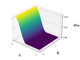
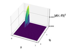
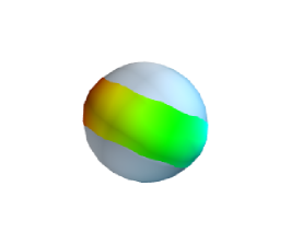
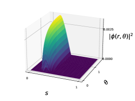
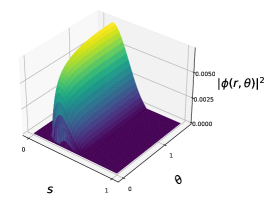
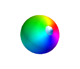
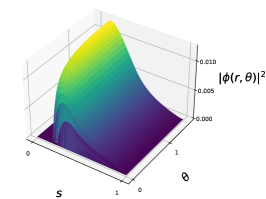
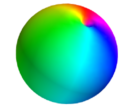
Figure 1: Different mixed star solutions having the same central density $\bar{\epsilon}_{c}=0.17$ and $\Gamma=1.0$. The upper solution was obtained for $\bar{w}=0.069$. The second row shows a $\bar{w}=0.078$ star. The third row shows a star with a frequency $\bar{w}=0.088$. The last row is for the limiting case $\bar{w}=0.0991$ star. It is important to notice that the radial coordinate is the compactified radius $s\in[0,1]$ and by columns, we plot $p_{NS}(s,\theta),|\phi(s,\theta)|^{2}$ and the contour plots show the energy densities for both parts, being the grey/blue spheres, the fermionic part and the multicolor contour the field energy density $|\phi(s,\theta)|^{2}$. The color in the bosonic part represents the phase.

From the analysis of fig. 1, we deduce several notable properties of mixed stars within the framework of our study. Each row in the figure is dedicated to a distinct star, with subsequent columns providing detailed visualizations of the variables $p_{NS}(s,\theta)$ and $|\phi(s,\theta)|^{2}$ across the $s,\theta$ grid. The final column offers a representation of both fermionic and bosonic energy densities, rendered in Cartesian coordinates. This structured presentation facilitates a comprehensive comparison of the physical characteristics inherent to each star, delineating the spatial distribution of gravitational potentials, pressure fields, and scalar field configurations. Moreover, the juxtaposition of fermionic and bosonic energy densities in the concluding column underscores the interplay between these fundamental components, highlighting their distribution and relative contributions within the composite structure of the mixed stars.

Despite the markedly different scenarios under consideration, the visual comparisons between the pressure within the neutron stars, $p_{NS}$, depicted in the first column, do not exhibit significant contrast. Although the numerical values characterizing $p_{NS}$ are distinctly different, a visual examination does not readily differentiate between the four cases. It is in the representations of the scalar field and the spatial energy density where the distinctions become pronounced.

Upon scrutinizing the second and third columns of fig. 1, we observe a clear differentiation in the scalar field distributions and their corresponding energy density manifestations, analyzed on a row-by-row basis. The initial star demonstrates the most pronounced scalar field distributions, which, when interpreted in terms of energy density distribution, reveals a slender torus of bosonic matter that envelops and intersects the NS exterior.

In the subsequent scenario, the expansion of the field distribution is evident, indicating that the torus now encompasses a larger portion of the NS. This expansion is indicative of an increase in total mass. The third scenario illustrates a significant enhancement in the field’s predominance, to the extent that the NS is almost completely cloaked in bosonic matter. The final depicted scenario reveals a mixed star configuration where the NS is entirely encased in bosonic matter, with the torus expanding to such a degree that it nearly forms a spherical shape.

These observations stress the intricate interplay between the scalar field distributions and the resultant energy density surfaces, highlighting the transition from a slim torus to an almost spherical envelope of bosonic matter. This transition reflects the varying degrees of interaction between the fermionic and bosonic components.

Computing the total masses for the family of solutions as a function of the parameters $M_{T}(\bar{w},\bar{\epsilon}_{c})$ allows us to study the region where the scalar field couples more strongly, leading to more massive stars.

Figure 2: Contour plots depicting the total masses as functions of the scalar field frequency and the central NS energy density are presented. The upper and lower plots display identical datasets, with the lower plot offering a magnified view of the region where the behavior of the bosonic component becomes more discernible.

In fig. 2 we represent solutions for the range of $\bar{w}$ between $0.085$ and $0.0993$. We explored, in fact, solutions for $\bar{w}\in[0.0685,0.0993]$, but for $\bar{w}<0.085$ the boson component contributes less than $2\%$ of the total mass, rendering them less relevant for our analysis.

We start the analysis by scrutinizing the upper plot in fig. 2, wherein the contour can be explained by splitting it into four principal regions. The first region is characterized by an exceedingly low NS energy density, where $e_{c}\sim(0,0.2)$. Solutions within this parameter space represent the existence threshold for NS, manifesting very low masses and failing to meet the requisite density and compactness criteria essential for sustaining a scalar field. This segment of the plot can be elucidated by drawing a parallelism with a mass-radius plot for NSs, specifically focusing on the segment where the mass is below $0.5M_{\odot}$ and the radii exceed 13 km. Additionally, an inspection of this region with respect to $\bar{w}$ reveals negligible variations despite alterations in the parameter, aligning with the inference that the solutions are derived under a scenario dominated by fermionic matter, even if the fermioninc component is itself small. This suggests that a certain mass threshold for NSs is imperative to facilitate a significant coupling with the scalar field.

The second region is distinctly demarcated by the contours, encompassing the solution space bounded by $\bar{w}\in(0.068,0.096)$ —excluding certain solutions at the lower limit of $\bar{w}$ to omit redundant information —and $\bar{e}_{c}\in(0.2,0.85)$. This domain exhibits solutions with neutron star masses in the range of $1.8-2.3~{}M{\odot}$. Notably, the solutions within this region display low sensitivity to variations in frequency and energy density, indicating that a broad parameter space converges to similar types of solutions. This implies a certain robustness or invariance in the NS characteristics within this specific range of parameters, reflecting an area of uniformity in the solution space.

The third region is situated in the right portion of the upper plot in fig. 2. It is characterized by a decrease in the total mass beyond $\bar{e}_{c}\sim 0.9$. This trend aligns with observations from prior studies on polytropic NSs and mixed fermion-boson stars (see for instance Di Giovanni et al. (2020a)) and was anticipated in our research. The influence of the field frequency on this behavior is evident, as the contours exhibit rounded borders, indicating a variation in mass with frequency. Analysis of this plot reveals that higher frequencies correlate with more massive solutions, which can be attributed to the increased coupling of the scalar field within the system, thereby leading to an increase of the total mass of mixed stars in this region.

Finally, the fourth region is the high frequency parameter space ranging almost all the data based on the $\bar{e}_{c}$. We define it for solutions with $\bar{w}\geq 0.096$ and $\bar{e}_{c}>0.2$. This region covers a wide range of data predicated on $\bar{e}_{c}$ and is prominently illustrated in the lower panel of fig. 2. Several critical insights can be derived from this solution domain.

Figure 3: We show the relation between the bosonic and total mass for our mixed stars data set. The upper and lower plots have the same data, but zoom the region of interest in the second one.

A pivotal observation is the attainment of maximum masses exceeding $4.5M_{\odot}$ within a small subregion, indicating the presence of exceptionally massive mixed star solutions. However, it is noted that these maximal mass values are not located at the extreme boundaries of the parameter space, as one could naively expect. Instead, there is a discernible decrease in mass beyond a specific neutron star energy density and scalar field frequency threshold. This behavior is visually represented by a narrow yellow band, flanked by green and blue regions, signifying that an increase in $\bar{w}$ and $\bar{e}_{c}$ beyond specific limits reduces the total mass. This phenomenon suggests a complex relation between the two significant parameters within this high-frequency region.

Another surprising behavior is found concerning the field frequency boundary. When increasing $\bar{e}_{c}$, the space of $\bar{w}$ where the code finds equilibrium solutions decreases linearly. Further, in this region an effect already described for the third region is stronger. We see how the contours describe a sort of central higher mass region that clearly decreases after going beyond the thresholds. This pattern suggests the formation of a peak in the mixed star mass that decreases on either side of these thresholds, illustrating a nuanced interplay between central energy density and field frequency in determining the total mass.

Additionally, higher values of $\bar{w}$ lead to a convergence of contours, making this region richer in terms of the variety of solutions. This behavior emphasizes the significant influence of the bosonic component on the equilibrium and structural characteristics of mixed stars within the high-frequency domain.

A possible explanation for this behavior is the following. Our fermionic matter models are rapidly rotating, and so are the bosonic parts for stars for which the field frequency is higher, as an increase in $\bar{w}$ means higher rotational frequency for bosonic stars. What we might be seeing here is a kind of rotational frequency synchronization relation for both the fermionic and bosonic parts and the mixed star reaches higher total masses and couples both matters in a better way if the bosonic and the fermionic parts tend to rotate in a comparable or equal manner. But a rigorous study will be done in a future work.

The subsequent fig. 3 shows the ratio between the mass of the bosonic part and the total mass obtained by summing the fermionic and bosonic contributions. This figure helps to clarify and expands on some of the above conclusions. The upper panel shows a broader range of solutions where we can identify solutions with less than a $10\%$ of bosonic content, shown in dark blue, and solutions where the BS part represents more than $60\%$ of the total mass in light green and yellow. It becomes clear from this plot that the medium-high energy density-high-frequency region is the part of the parameter space where the bosonic contribution becomes important.

We can go even further in the analysis if we zoom into the above-mentioned region of interest. The lower panel in fig. 3 shows this region in more detail. The first assessment we can make is related to the high variability of the space of solutions, meaning that the solutions in this area are strongly affected by any variation in $\bar{w}$. We also checked that the spectra of solutions decrease for the frequency when $\bar{e}_{c}$ increases. Additional comments can be made about the maximal bosonic mass found in our data set. There is a tiny region for non-extremal high frequencies and medium NS energy densities, where the bosonic component reaches values above $60\%$ of the total mass. Moving beyond these values of the parameters, the bosonic contribution to the total mass decreases significantly.

It is important to acknowledge that the study of the higher spectrum of solutions is constrained by potential numerical challenges. Our computational model is designed to solve problems within specific boundary conditions. However, an unregulated increase in the number of bosons could lead to a scenario where asymptotic flatness is violated. In such cases, the code struggles to converge to a meaningful equilibrium solution as the fundamental assumptions of the model are violated.

This limitation underscores the intricate balance required in numerical simulations, especially when dealing with systems where the interplay of various components —such as the neutron star and boson star elements— can lead to complex and, at times, unpredictable outcomes. The inability to reach a broader spectrum of solutions highlights the system’s sensitivity to boundary conditions and the need for a careful control of parameters to ensure the reliability and relevance of the simulated solutions.

V.2 Presence of ergoregions

The ergoregion instability appears in any system with ergoregions and no horizons. For some models of rapidly rotating NS, it was shown that ergoregions can arise when dealing with certain EOS Tsokaros et al. (2019) where typical instability time scales are shown to be larger than the Hubble time. In these cases, the ergoregion instability is too weak to affect the star’s evolution. This conclusion changes drastically for ultracompact stars. Depending on the compactness, it was found that instability time scales ranging from seconds to even weeks Cardoso et al. (2008). Indeed, a rigorous study was done around various types of exotic compact objects Maggio et al. (2019). Furthermore, BSs has been proven to support ergoregions depending on the self-interaction governing the field Vaglio et al. (2022). Those fast-spinning, massive BSs are directly related to our mixed stars.

On the other hand, the mixed stars we have obtained with the polytropic EOS discussed in this work, with $\Gamma=1.0$, and for any value of $\bar{w}$ did not present any ergoregion. However, considering different polytropic indexes resulted in drastic changes in the compactness of our solutions, and some of them showed this kind of region where no particle can remain at fixed $r,\theta$ and $\psi$. To further underline this point, and going beyond the polytropic EOS, we present in fig. 4 a solution obtained for a rather realistic, tabulated EOS Adam et al. (2020) where we appreciate two changes in the sign of $g_{tt}$, which translates into the existence of an ergoregion, demonstrating that mixed stars can also support ergoregions. Firstly, we show their existence for some of our results, making a clear connection with Tsokaros et al. (2019); Vaglio et al. (2022). Secondly, this result anticipates a future research line since our solver is capable of using tabulated EOS. In future work, therefore, we will be able to analyze in detail and discuss more realistic models from the point of view of the NSs.

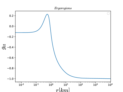
Figure 4: For the EOS presented in Adam et al. (2020) and some very specific parameters, we have found ergoregions with toroidal topology in our mixed star solutions. These manifest as a change in the $g_{tt}$ sign.

VI Fermion-Boson stars in gravitational-wave astronomy

While alternative scenarios have been proposed Bustillo et al. (2021); Calderon Bustillo et al. (2023), the vast majority of current GW detections of compact binaries are perfectly described by that of mergers of black holes and/or NS Abbott et al. (2019, 2021a); Collaboration and the Virgo Collaboration (2021); Abbott et al. (2021b). There exist, however, observations that challenge the assumed characteristic masses of these objects. For instance, the event GW190814 Abbott et al. (2020c) involves a compact object of around $2.6M\odot$, falling in the so-called “lower-mass black-hole gap”, where the formation of black holes from stellar-collapse is prevented. While scenarios involving primordial black holes Vattis et al. (2020); Clesse and Garcia-Bellido (2020) and dark matter Lee et al. (2021); Das et al. (2021b) have been proposed to explain such event, fermion-boson stars can also populate such mass range, offering an alternative scenario Di Giovanni et al. (2022c). While we are far from performing actual numerical simulations of mergers of these objects, we anticipate two potential avenues to confirm or discard such an option. First, GWs emitted during the end stages of the inspiral phase will contain information about the characteristic tidal deformability of these objects. Second, the bosonic part of the star will affect both the nature of the final object, most likely making it collapse into a black hole due to the increased mass of the binary in comparison to the case of pure NS binaries, and any potential post-merger emission. In both cases, third-generation detectors such as Einstein Telescope Punturo et al. (2010); Hild et al. (2010), Cosmic Explorer Reitze et al. (2019); Abbott et al. (2017c) or NEMO Ackley et al. (2020) will be needed to access the corresponding information.

The expanded array of options provided by our mixed solutions offers essential insights that could address the inconsistencies observed in recent multi-messenger observations and nuclear physics experiments concerning NS masses and radii. Notably, our developed solutions exhibit significant coherence with multi-messenger data, p.e., by populating the lower-mass black hole gap with our hypothetical compact fermion-boson stars, in the line with the discussion in Di Giovanni et al. (2022c). This coherence extends beyond the previously mentioned GW to include X-ray pulsars PSR J0030+0451 Miller et al. (2019b) and PSR J0740+6620 Miller et al. (2021). Additionally, these solutions are in alignment with the nuclear physics constraints determined by the PREX-2 experiment Reed et al. (2021).

We note that the above statements, including the viability of isolated rotating mixed stars and of compact mergers involving fermion-boson stars, crucially depend on a few assumptions that we outline next. Despite the positive outcomes achieved and the potential relevance to the mass-gap context, it is imperative to exercise a degree of caution due to the specific and limiting assumptions that were applied to derive our solutions. First of all, for the stars composed of fermionic matter we mainly employed polytropic EOS in the presented work rather than other tabulated, realistic EOS. This implies that our models should be considered approximations from the outset. Nonetheless, as we have indicated in the previous section, and in spite of not presenting it in this work, our solver can be readily generalized to accommodate tabulated EOS. Undoubtedly, the most significant limitation arises from employing the Ryan-Pani-Vaglio approximation for the scalar field Vaglio et al. (2022); Ryan (1997b). This approach restricts the value range of the coupling constants or the adoption of different potentials. By relying on this approximation, we cannot guarantee that the use of other potentials or constants within another algorithm framework would not alter the solutions we obtain. Nevertheless, considering that the quartic potential with a high coupling constant represents one of the assumed stable scenarios Siemonsen and East (2021); Di Giovanni et al. (2020b), we can assert with moderate confidence that the use of this approximation is justifiable, particularly concerning the stability of bosonic matter. In the absence of dedicated stability studies, definitive assertions cannot be made within this framework. However, we have grounds to hypothesize that our objects may possess inherent stability. This potential for stability is inferred from the fact that both the fermionic and bosonic components, when examined independently, have demonstrated stable characteristics.

In conclusion and by way of anticipation, we venture to suggest that our model, despite its approximate nature, is likely not far removed from an exact representation. Solving the complete system with realistic EOS and integrating the scalar field without any approximation will undoubtedly alter at a certain degree the total mass and the relative proportions between fermionic and bosonic masses. However, we posit that the nature of the solutions will closely resemble our findings, both in terms of the object’s geometry or topology and the total magnitude or range of the masses.

VII Conclusions

We have presented a new kind of hypothetical compact object: a fully spinning mixed fermion-boson star with a specific bosonic self-interaction, valid within the large self-coupling regime. The Einstein equations for the axisymmetric system, sourced by a mixed stress-energy tensor eq. 18, have been solved by a $\mathcal{C}$-code that takes the RNS Cook et al. (1992) as a base. Due to the large number of parameters defining this kind of system, the available zoo of solutions is large. For this reason, we present only one complete family of configurations, as it is the first time that this kind of object is treated in depth.

We delineate the theoretical framework incrementally, before integrating it into a cohesive system, to elucidate our conceptualization of the hypothetical astrophysical object. Subsequently, we systematically detail the implementation of the intricate algorithm employed for solving this integrated system. Following the derivation of accurate expressions intended to quantify observable magnitudes, we conducted simulations of several representative cases. These simulations, grounded in carefully selected initial conditions, facilitated the exploration of the most plausible astrophysical scenarios. Specifically, these scenarios involve a NS that variably accretes bosons, thereby illustrating the nature of such astrophysical objects. Not only were the metric potentials and scalar field behaviors elucidated for a selection of distinct and representative cases, but volumetric representations of energy densities for both types of matter were also constructed and analyzed. These visualizations provide insights into the comprehensive matter distributions of these astrophysical entities within spatial dimensions. Furthermore, the analysis allows for the observation of a conventional, flattened spherical spinning NS encased within a toroidal distribution of the scalar field, highlighting the complex interplay between the NS and surrounding scalar fields.

Upon fixing specific parameters, such as the oblateness of the inner NS, the harmonic index, polytropic variables, and the mass of the bosons, we derived a comprehensive suite of solutions by modulating the internal bosonic scalar field frequency and the central energy density of the NS. It is important to underscore that the simulated scenarios invariably commence with a purely static NS as the initial condition, resulting in configurations that are, in general, more enriched in fermionic content. This outcome aligns with what is astrophysically considered to be the most likely scenario.

Our findings suggest that the novel astrophysical entities introduced in this study are capable of achieving greater masses in some scenarios, particularly when the frequency $w$ closely approaches but remains smaller than the value of $\mu_{b}$, and when the central energy density increases within specific bounds, rather than arbitrarily. Consequently, it becomes feasible to form objects with masses surpassing $3M_{\odot}$, potentially extending up to $4M_{\odot}$.

A key focus of our analysis also lies in contrasting the contribution of bosonic matter to the total mass, thereby elucidating the significance and proportion of scalar bosonic matter within the entire astrophysical entity. Despite an inherent predominance of fermionic matter, particularly in regions associated with higher masses, our observations reveal a convergence towards equilibrium in the percentage composition of both bosonic and fermionic natures. Notably, we identify limiting cases where over $50\%$ of the mass can be attributed to the BS component. Our investigation further extended to the presence of ergoregions, yielding positive outcomes. These findings were realized after the application of an advanced, albeit not comprehensively examined, methodology involving the use of realistic EOS during the integration process of the mixed system.

One of the most significant contributions of our results could lie in their potential to elucidate certain astrophysical phenomena currently interpreted as mass-gap black holes, specially among GW observations. The compact objects detailed in this manuscript, though not entirely realistic owing to the adoption of polytropic models and large self-interaction constants for NS and BS components respectively, illuminate a novel avenue for extending these models to more encompassing and plausible scenarios. Our analysis, bolstered by additional verifications not detailed herein, suggests that incorporating realistic EOS could diversify the spectrum of solutions. This includes the possibility of achieving higher masses in certain instances, altering the scalar field configurations, and fostering varied fermion-boson equilibria, wherein the NS component primarily functions as a core. However, given the ongoing nature of our investigation, we reserve more bold conclusions for future work.

Our ongoing research endeavors are directed towards intriguing expansions of our previous work. Notably, the incorporation of realistic EOS has been identified as a viable direction, though it remains under-explored in a systematic context. An immediate enhancement under consideration involves transcending the approximation of large self-interaction coupling constants to address the dynamics of a fully realized scalar field, integrated via a generalized Stress-Energy tensor. Furthermore, the exploration of varied self-interaction potentials for the BS component presents a fertile ground for additional inquiry. The extension of our methods to encompass spinning fermion-Proca stars is another avenue of interest. There are also promising insights into the study of stability and evolutionary trajectories of these novel mixed compact objects. Moreover, the investigation into Universal Relations, the multipolar structure, and the determination of deformability parameters for these entities are anticipated to yield significant implications. Such advancements not only augment our understanding of compact astrophysical objects but also enhance the theoretical framework necessary for interpreting their observational signatures.

Appendix A Additional equations

We introduce a series of equations that, being of main interest, we do not add to the text for clarity of reading. First of all we show the sources for the pure spinning NS case:

$$\begin{split}&S_{\rho}(r,\mu)=e^{\gamma/2}\left[8\pi e^{2\alpha}\left(\rho_{0}+\rho_{i}+P\right)\frac{1+v^{2}}{1-v^{2}}+r^{2}(1-\mu^{2})e^{-2\rho}\left(\omega_{,r}^{2}+\frac{(1-\mu^{2})}{r^{2}}\omega^{2}_{,\mu}\right)+\right.\\ &\left.\frac{1}{r}\gamma_{r}-\mu\gamma_{,\mu}+\frac{\rho}{2}\left\{16\pi e^{2\alpha}P-\gamma_{,r}\left(\frac{1}{2}\gamma_{,r}+\frac{1}{r}\right)-\frac{1}{r^{2}}\gamma_{,\mu}\left(\frac{1-\mu^{2}}{2}\gamma_{,\mu}-\mu\right)\right\}\right],\end{split}$$ (58)

$$S_{\gamma}(r,\mu)=e^{\gamma/2}\left[16\pi e^{2\alpha}P+\frac{\gamma}{2}\left(16\pi e^{2\alpha}P-\frac{1}{2}\gamma_{,r}^{2}-\frac{1-\mu^{2}}{2r^{2}}\gamma_{,\mu}^{2}\right)\right]$$ (59)

$$\begin{split}&S_{\omega}(r,\mu)=e^{(\gamma-2\rho)/2}\left[-16\pi e^{2\alpha}\frac{(\Omega-\omega)(\rho_{0}+\rho_{i}+P)}{1-v^{2}}+\right.\\ &\left.\omega\left\{-8\pi e^{2\alpha}\frac{(1+v^{2})(\rho_{0}+\rho_{i})+2v^{2}P}{1-v^{2}}-\frac{1}{r}\left(2\rho_{,r}+\frac{1}{2}\gamma_{,r}\right)+\frac{\mu}{r^{2}}\left(2\rho_{,\mu}+\frac{1}{2}\gamma_{,\mu}\right)+\right.\right.\\ &\left.\left.\frac{1}{4}(4\rho_{,r}^{2}-\gamma_{,r}^{2})+\frac{1-\mu^{2}}{4r^{2}}(4\rho_{,\mu}^{2}-\gamma_{,\mu}^{2})-r^{2}(1-\mu^{2})e^{-2\rho}\left[\omega_{,r}^{2}+\frac{(1-\mu^{2})}{r^{2}}\omega_{,\mu}^{2}\right]\right\}\right]\end{split}$$ (60)

For the fourth equation, the one involving the $\alpha$ function, we have,

$$\begin{split}&\alpha_{,\mu}=\\ &-\frac{1}{2}\left(\rho_{,\mu}+\gamma_{,\mu}\right)-\left\{\left(1-\mu^{2}\right)\left[1+r\gamma_{,r}\right]^{2}+\left[\mu-\left(1-\mu^{2}\right)\gamma_{,\mu}\right]^{2}\right\}^{-1}\left[\frac{1}{2}\left[r^{2}\left[\gamma_{,rr}+\gamma_{,r}^{2}\right]\right.\right.\\ &\left.-\left(1-\mu^{2}\right)\left(\gamma_{,\mu\mu}+\gamma_{,\mu}^{2}\right)\right]\left[-\mu+\left(1-\mu^{2}\right)\gamma_{,\mu}\right]+r\gamma_{,r}\left[\frac{1}{2}\mu+\mu r\gamma_{r}+\frac{1}{2}\left(1-\mu^{2}\right)\gamma_{,\mu}\right]+\\ &\left.+\frac{3}{2}\gamma_{,\mu}\left[-\mu^{2}+\mu(1-\mu^{2})\gamma_{,\mu}\right]-r\left(1-\mu^{2}\right)\left(\gamma_{,r\mu}+\gamma_{,r}\gamma_{,\mu}\right)\left(1+r\gamma_{,r}\right)-\frac{1}{4}\mu r^{2}\left(\rho_{,r}+\gamma_{,r}\right)^{2}-\frac{r}{2}\left(1-\mu^{2}\right)\left(\rho_{,r}+\gamma_{,r}\right)\left(\rho_{,\mu}+\gamma_{,\mu}\right)\right.\\ &\left.+\frac{1}{4}\mu\left(1-\mu^{2}\right)\left(\rho_{,\mu}+\gamma_{,\mu}\right)^{2}-\frac{r^{2}}{2}\left(1-\mu^{2}\right)\gamma_{,r}\left(\rho_{,r}+\gamma_{,r}\right)\left(\rho_{,\mu}+\gamma_{,\mu}\right)+\frac{1}{4}\left(1-\mu^{2}\right)\gamma_{,\mu}\left[r^{2}\left(\rho_{,r}+\gamma_{,r}\right)^{2}-\left(1-\mu^{2}\right)\left(\rho_{,\mu}+\gamma_{,\mu}\right)^{2}\right]\right.\\ &\left.+\left(1-\mu^{2}\right)e^{-2\rho}\left\{\frac{1}{4}r^{4}\mu\omega_{,r}^{2}+\frac{1}{2}r^{3}\left(1-\mu^{2}\right)\omega_{,r}\omega_{,\mu}-\frac{1}{4}r^{2}\mu\left(1-\mu^{2}\right)\omega_{,\mu}^{2}+\frac{1}{2}r^{4}\left(1-\mu^{2}\right)\gamma_{,r}\omega_{,r}\omega_{,\mu}\right.\right.\\ &\left.\left.-\frac{1}{4}r^{2}\left(1-\mu^{2}\right)\gamma_{,\mu}\left[r^{2}\omega_{,r}^{2}-\left(1-\mu^{2}\right)\omega_{,\mu}^{2}\right]\right\}\right]\end{split}$$ (61)

We introduce as an example the $\rho$ equation in the KEH seminal paper, in terms of the three-dimensional Green function previous to the expansion. The integral formula for the potential is written in $(r,\mu)$ variables:

$$\rho\sim\int_{0}^{\infty}dr^{\prime}\int_{-1}^{1}d\mu^{\prime}\int_{0}^{2\pi}d\psi^{\prime}r^{\prime 2}S_{\rho}(r^{\prime},\mu^{\prime})\frac{1}{|\textbf{r}-\textbf{r'}|},$$ (62)

and we show the series expansion for the Green function,

$$\frac{1}{|\textbf{r}-\textbf{r'}|}=\sum_{n=0}^{\infty}f_{n}^{\prime 2}(r,r^{\prime})\left[P_{n}(\cos\theta)P_{n}(\cos\theta^{\prime})+2\sum_{m=1}^{n}\frac{(n-m)!}{(n+m)!}P_{n}^{m}(\cos\theta)P_{n}^{m}(\cos\theta^{\prime})\cos m(\psi-\psi^{\prime})\right]$$ (63)

where,

$$f_{n}^{2^{\prime}}(r,r^{\prime})=\begin{cases}(1/r)(r^{\prime}/r)^{n},&for\hskip 28.45274ptr^{\prime}/r\leq 1\\ (1/r^{\prime})(r/r^{\prime})^{n},&for\hskip 28.45274ptr^{\prime}/r>1.\\ \end{cases}$$ (64)