SHIVA and SHAKTI:
Presumed Proto-Galactic Fragments in the Inner Milky Way
Abstract
Using Gaia DR3 astrometry and spectroscopy, we study two new substructures in the orbit-metallicity space of the inner Milky Way: Shakti and Shiva. They were identified as two confined, high-contrast overdensities in the distribution of bright () and metal-poor () stars. Both have stellar masses of , and are distributed on prograde orbits inside the Solar circle in the Galaxy. Both structures have an orbit-space distribution that points towards an accreted origin, however, their abundance patterns – from APOGEE – are such that are conventionally attributed to an in situ population. These seemingly contradictory diagnostics could be reconciled if we interpret the abundances [Mg/Fe], [Al/Fe], [Mg/Mn] vs. [Fe/H] distribution of their member stars merely as a sign of rapid enrichment. This would then suggest one of two scenarios. Either these prograde substructures were created by some form of resonant orbit trapping of the field stars by the rotating bar; a plausible scenario proposed by Dillamore et al. (2023). Or, Shakti and Shiva were proto-galactic fragments that formed stars rapidly and coalesced early, akin to the constituents of the Poor Old Heart of the Milky Way; just less deep in the Galactic potential and still discernible in orbit space.
1 Introduction
One focus of modern astrophysics is to understand how massive galaxies, such as our Milky Way, formed and evolved. To address this broad theme with observations of the present epoch Universe, it has proven powerful to take the Milky Way itself as a galaxy model organism for which to map – and then eventually understand – the detailed age-orbit-abundance distribution of its stars. This constrains when and on which orbits its stars formed, how the stellar birth material became gradually enriched, and which dynamical processes – e.g. mergers or secular evolution – shaped the Galactic structure. The importance of various processes must depend both on the epoch and on the Galactocentric radius (or potential well depth) at which they occur.
One of the most striking observations of our Galaxy is how dramatically age, metallicity, and orbits of stars are connected (e.g., Bland-Hawthorn & Gerhard 2016). The stellar body is dominated by a rotation-dominated, disky distribution (e.g., Rix & Bovy 2013; Helmi 2020) that shows a bimodal density distribution in the [Fe/H]-[/Fe] plane (e.g. Bensby et al., 2014), where both the kinematics and the spatial structure depend strongly on both [Fe/H] and [/Fe] (e.g. Bovy et al., 2012). Basically all these stars with disk-like kinematics have [M/H] (e.g., Mackereth et al. 2019). The central portions of our Galaxy ( kpc) are dominated by a bar (Blitz & Spergel, 1991) and a central spheroid, dominated by random motions and a wide range of metallicities (e.g. Ness et al., 2013; Belokurov & Kravtsov, 2022; Rix et al., 2022). The arguably smallest component by stellar mass, but the largest by spatial extent (to kpc) is the stellar halo with [M/H]. At least beyond kpc, it is predominately composed of unbound ‘debris’ of tidally disrupted satellite galaxies (Ibata et al., 1994; Helmi et al., 1999; Bell et al., 2008; Newberg et al., 2009; Belokurov et al., 2018; Helmi et al., 2018; Myeong et al., 2019; Koppelman et al., 2019a; Yuan et al., 2020; Naidu et al., 2020; Necib et al., 2020; Malhan, 2022; Tenachi et al., 2022).
Parsing the overall stellar orbit–abundance distribution into an extensive set of individual components has been a long tradition, as each of them may represent a discrete event or regime in our Galaxy’s formation history. In particular, it has become established to categorise each component or substructure as either born from gas already within the Milky Way’s dominant potential well (dubbed in-situ) or born within a (at the time) distinct subhalo (or satellite galaxy) that was later accreted into the Milky Way.
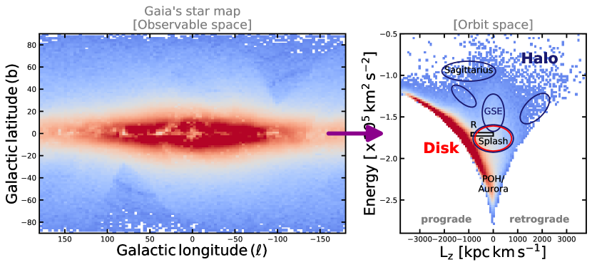
Among old ( Gyrs) stellar populations in the Milky Way, the prototypical in-situ population is the -enhanced or thick disk. This inference is based on the disk-like kinematics that reflects the settling of the stars’ birth gas in the Milky Way’s main potential well (e.g. Birnboim & Dekel, 2003; Stern et al., 2021), starting ago (Xiang & Rix, 2022). When looking at these stars in the plane of orbital parameters, their distribution follows the line of circular, in-plane orbits (see Fig. 1), though not exactly owing to their substantive velocity dispersion. And this assessment of an in-situ origin is based on the abundance patterns: these stars are enhanced in [Mg/Fe] and [Mg/Mn] and show a rapid rise of [Al/Fe] with [Fe/H]. All of these are taken as signatures of rapid enrichment that presumably requires high densities and a deep potential well (Hawkins et al., 2016; Belokurov & Kravtsov, 2022).
Among the stellar halo components, the Gaia-Sausage-Enceladus (henceforth GSE) population (Helmi et al., 2018; Belokurov et al., 2018) exemplifies an accreted population (see Fig. 1; right panel). The very low angular momentum and large apocenters of their orbits cannot be readily explained by an in-situ origin, and the low- abundance patterns resemble those of the ‘surviving’ dwarfs satellites of the Milky Way and point toward slow enrichment in a more diffuse potential well (Wyse, 2016; Hasselquist et al., 2021).
Yet, when looking in detail at the very early phases of our Galaxy’s evolution (say ago), this in-situ vs. accreted distinction may become practically ambiguous and conceptually subtle. For instance, there is the “Splash” population (see Fig. 1), identified by Bonaca et al. (2017); Di Matteo et al. (2019); Belokurov et al. (2020) that has been termed the “metal-rich in-situ” halo: its orbits are radial (hence halo-like, favouring and accreted origin), but the population is metal-rich with [M/H] and -enhanced, pointing towards an in-situ scenario. But both properties can be understood if its population arose from stars that were kicked out of the early, nascent in-situ disk into radial orbits during an early collision with some massive merger.
Recent studies of ancient stars in the inner Galaxy (Kruijssen et al., 2019; Belokurov & Kravtsov, 2022; Rix et al., 2022; Horta et al., 2022; Conroy et al., 2022) have identified a dynamically hot population of tightly-bound stars, namely the Poor Old Heart of the Milky Way (or Aurora), henceforth POH (see Fig. 1). Most of these stars show the chemical signatures of rapid enrichment (i.e., these stars are enhanced in [Mg/Fe] and [Mg/Mn] and show a rapid rise of [Al/Fe] with [Fe/H]) that are conventionally attributed to an in-situ origin. Simulations of galaxy formation (e.g., Renaud et al. 2021) suggest that this component originated presumably from the coalescence of several proto-Galactic fragments that were of comparable, though not equal, mass. Whether at such early phases, it is useful to attribute the term in-situ for only one of these presumed protogalactic fragments (Belokurov & Kravtsov, 2022) is not clear (cf. Rix et al., 2022; Conroy et al., 2022). Nonetheless, the abundance pattern of these stars may serve as a reminder that they only imply rapid enrichment (which may require high star formation rates, deep potential wells and high densities), rather than as a direct indicator of the dynamical pre-history.
But also the inference path from a particular orbit distribution to, say, an accreted origin may not be straightforward or unique. For instance, as mentioned above, the “Splash” population has halo-like orbits and appear to favour an accreted origin; but, it actually comprises metal-rich stars with [M/H] that suggest it was the earliest part of the -enhanced disk whose stars were dramatically stirred during an early, quite massive merger. Likewise, the “R” feature indicated in Fig. 1, which represents ridge-like overdensity of stars, may lend itself to the interpretation as an accreted population. But Dillamore et al. (2023) showed that this feature comprises both metal-rich and metal-poor stars and their orbits lie somewhere between disk- and halo-like. Given that these stars’ azimuthal orbit frequency coincides with that of the Galactic bar, this orbit-space substructure can be very plausibly attributed to the trapping of the (inner) halo stars in bar resonances.
In this study, our primary goal is to examine the (inner) Milky Way’s ()–[M/H] space, using the recent Gaia DR3–based XGBoost dataset, (Rix et al., 2022; Andrae et al., 2023, A23), to look for previously unrecognised substructures. In doing so, we identified two orbit-abundance space overdensities that we call Shakti and Shiva, and show these possess very intriguing properties that send “mixed messages” about their in-situ or accreted origin. To this end, Section 2 describes the data used. Section 2.2 details our method to compute the orbital parameters of the stars. In section 3, we analyze the () distribution of stars in different slices of [M/H], thereby identifying Shakti and Shiva. Section 4 and Section 5 present the characterization of these stellar populations. In Section 6, we lay out possible origin scenarios for these two populations. We finally conclude in Section 7.
2 Data
To explore the Milky Way’s stellar ()[M/H] space, we require for each star [M/H] information and a complete 6D phase-space measurement, i.e., its sky position (), parallax (, which can be inverted to obtain the heliocentric distance), proper motions () and line-of-sight velocity ().
2.1 XGBoost dataset
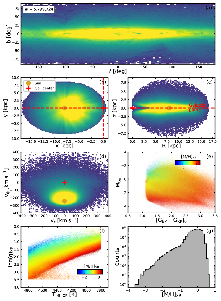
For this, one of the most extensive and well-vetted data sets is the recent Gaia DR3–based XGBoost catalogue (Rix et al., 2022; Andrae et al., 2023, A23). A23 provides data-driven XGboost estimates of stellar metallicity , surface gravity and effective temperature for million sources. These are based on their Gaia DR3 low-resolution BP/RP (or, XP) spectra, after being trained on stellar parameters from APOGEE that have been augmented by a set of very metal-poor stars. Although all of these stars have Gaia DR3’s 5D astrometry, only brighter sources (with mag) also have Gaia RVS velocities. A23 combines one of the most extensive data set with 6D phase-space with [M/H] that are robust, precise, and vetted against a number of external catalogs, such as APOGEE DR17 (Abdurro’uf et al., 2021), GALAH DR3 (Buder et al., 2021), LAMOST DR7 (Zhao et al., 2012) and SEGUE (Yanny et al., 2009). In our analysis, we restrict ourselves to only those stars with , K K and , because in this range XGBoost’s [M/H] estimates are most robust and precise (with ). Even with these quality cuts, this A23 subset contains times more stars compared to APOGEE DR17 and LAMOST DR7, times more stars compared to GALAH DR3 and times more stars than in SEGUE.
We apply additional quality to ensure good Gaia astrometry (similar to Malhan, 2022): (1) parallax_over_error; this quality cut ensures that our resulting sample contains well-measured parallaxes with relative parallax error of . Effectively, it also ensures that and that the estimated heliocentric distances are physical. We correct for the parallax zero-point of each star as (Lindegren et al., 2021). (2) phot_bp_rp_excess_factor; this moderate cut removes stars with strong color excess that occurs in the very crowded regions of the Galaxy (for normal stars, phot_bp_rp_excess_factor, Arenou et al. 2018). (3) ruwe; this value has been prescribed as a quality cut for “good” astrometric solutions by Lindegren et al. (2021). This results in a sample of stars.
Finally, we excise all the stars that lie within five tidal radii of the globular clusters (listed in Harris 2010) in the 2D projection space. This removes stars.
Our final ‘base’ dataset comprises stars, and its overview is provided in Fig. 2. We correct for dust extinction using Schlegel et al. (1998) maps and assuming the extinction ratios , , (as listed on the web interface of the PARSEC isochrones, Bressan et al. 2012). Henceforth, all magnitudes and colors refer to these extinction-corrected values.
2.2 Orbits
To compute the orbital parameters of stars (such as , , etc), we need to transform their heliocentric phase-space measurements into Galactocentric Cartesian coordinates. This is achieved using the Sun’s Galactocentric location as (Gravity Collaboration et al., 2018) and the Sun’s Galactocentric velocity as (Drimmel & Poggio, 2018). Next, the Galactic potential is set up using the McMillan (2017) model, which is a static and axisymmetric model comprising a bulge, disk components and an NFW halo. With this potential, we compute the orbital parameters, using the galpy module (Bovy, 2015).
3 New stellar structures in space:
Shakti and Shiva
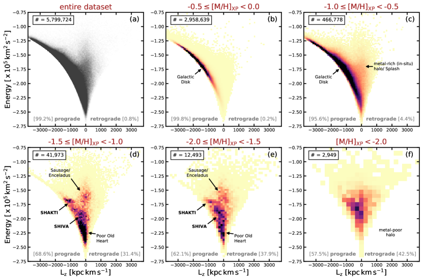
Fig. 3 shows the () orbit distribution of these stars in different slices, i.e. . Foremost, this Figure illustrates the known fact that the stellar orbit distribution depends dramatically on their metallicity, with the Galactic disk(s) dominating at (see panels and ). It also shows clearly some of the well-established low-metallicity ‘sub-structures’, such as the metal-rich in-situ halo/Splash (Bonaca et al. 2017; Di Matteo et al. 2019; Belokurov et al. 2020, visible in the panel ), GSE merger debris (Belokurov et al. 2018; Helmi et al. 2018, visible in the panels and ) and POH (Belokurov & Kravtsov 2022; Rix et al. 2022, visible in the panels and ).
Panels and of Fig. 3 (which together correspond to the metal-poor regime ) reveal the presence of three prominent substructures that are well confined in space. One of them with net corresponds to the known GSE structure. The other two prograde substructures at and at have previously not been observed as such prominent overdensities or appreciated as possible substructures. They are the focus of the present work, and for brevity, we denote them as Shakti and Shiva respectively111In Hindu philosophy, Shiva – Shakti are the divine couple and their union (i.e., shivashakti) gives birth to the whole macrocosm. The goddess Shakti represents the purest form of energy and the god Shiva (one of the trinity gods) represents consciousness.. The fact that these substructures are observed here for the first time with such high contrast, owes to the novel richness of the XGBoost dataset.
In the remaining study, we characterize the stellar populations of Shakti and Shiva and aim to understand their nature and origin (i.e., in-situ or accreted). At this juncture, it is important to note that the location of Shakti is similar to two previously identified substructures: the ridge-like component pointed out in Dillamore et al. (2023), who attribute them to halo stars that got spun up as they got trapped in the resonances of the Galactic bar (see our Fig. 1); and also a sparse population of metal-poor disk stars (e.g., Carollo et al. 2019; Naidu et al. 2020). To what extent these substructures are identical, overlapping or connected with Shakti is a question we address in Section 6.
4 Characterization of Shakti
Below, Section 4.1 describes our procedure to select the Shakti population, Section 4.2 details its chemo-dynamical properties and in Section 4.3 we compute its stellar mass.
4.1 Selection of Shakti stars
We select Shakti stars drawing on simple visual inspection of the distribution, inspired by the high-contrast appearance among low-metallicity stars (see panel of Fig. 3). Initially, we had tried for automated and systematic selection by employing some detection algorithms (namely, ENLINK, Sharma & Johnston 2009, and Gaussian mixture model, Pedregosa et al. 2011) and also experimented with different data sub-spaces (e.g., the 2D space, the 3D action space, the 4D space, the 3D space). We did not find that any of these served our specific purposes better than selection “by hand”.
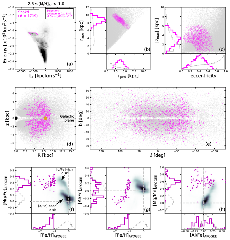
To select the Shakti population, we use the base data and restrict ourselves in the metallicity range and then retain only those stars that lie inside a 2D polygon described by four vertices as , , , ; the units are in []. This polygon best describes this population. The [M/H] range is in concordance with the [M/H] slices in which we identify Shakti in Fig. 3, and we especially probe the low–[M/H] range to gather even the very metal–poor stars. This selection results in stars.
| Shakti | Shiva | |||
| Parameters | Median | Spread | Median | Spread |
| eccentricity | ||||
4.2 Orbital and chemical properties of Shakti
Fig. 4 shows the distribution of the Shakti stars in the orbital space, spatial coordinates and chemical space. These distributions are quantified in Table 1, with uncertainties derived from bootstrap re-sampling. The basic properties can be summarized as follows.
Shakti stars orbit the Milky Way within the Galactocentric distance range of (Fig. 4, panel ); they reach away from the Galactic plane, and have moderate eccentricities of . Furthermore, these stars are well phase-mixed in the Galaxy (as shown in the and distributions).
We now turn to understanding Shakti’s detailed abundance patterns. We initially had selected Shakti members via . Now we aim to construct the detailed element ratios that can serve as diagnostics to differentiate Galactic populations (e.g., Hawkins et al. 2015; Belokurov & Kravtsov 2022). Since Gaia DR3 cannot deliver these222Gaia DR3 RVS provides individual element abundances essentially only for stars with [M/H] (Recio-Blanco et al., 2023)., we cross–match the Gaia-identified Shakti sample members with SDSS/APOGEE DR17 (Abdurro’uf et al., 2021; Almeida et al., 2023) to obtain [Fe/H], [Mg/Fe], [Al/Fe], [Mg/Mn]. In so doing, we find stars possessing [Fe/H] and [Mg/Fe] measurements. And of these, only stars possess [Al/Fe] measurements and stars possess [Mg/Mn] measurements.
Shakti stars are metal–poor, with an MDF that ranges from [Fe/H] to . The stars are all Fe]-enhanced, they show a tight relation in the [Al/Fe]–[Fe/H] plane, and of stars have [Al/Fe] (Fig. 4, panel , and ). Note that the [Fe/H]–[Al/Fe] relation is remarkably tight. The reason behind this is unclear, however, but it may be pointing towards a single, chemically simple origin for the Shakti stars, rather than a mix of different populations. While CMD-based analyses are generally quite useful to study stellar populations, here this is not very helpful for two reaons: all Shakti stars were chosen to be metal-poor, and hence by implication old, population of giant stars (see Section 2 and panels and of Figure 2). Second, for most members the parallaxes are not precise enough to enable meaninful age estimates.
How the above properties of Shakti relate to its nature and origin is discussed below in Section 6 (together with that of Shiva).
4.3 Shakti’s Stellar Mass
Obviously, the sample members that we attribute to Shakti are a highly biased subset of that structure’s stars, biased in luminosity and orbital phase.
If Shakti reflected an accreted satellite, we could employ the much-used mass-metallicity relation for dwarf galaxies (Kirby et al., 2013). Adopting a mean [Fe/H]APOGEE for Shakti would imply , as this mean metallicity resembles that of the known WLM dwarf galaxy, which has [Fe/H] and (Zhang et al., 2012; McConnachie, 2012). It is important to note that this [Fe/H]– relation possesses significant scatter and also a redshift dependence (i.e., higher masses at higher redshifts at fixed [Fe/H], e.g., Zahid et al. 2014; Ma et al. 2016).
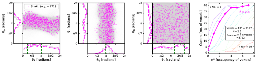
Alternatively, we can simply count Shakti’s stars, accounting for the fact that we only consider giants; and that we will not see its members at all orbital phases. Indeed, Frankel et al. (2023) suggested to exploit the fact that for phase-mixed structures the distribution in all three orbital angles is expected to be uniform. If we can estimate the “angle incompleteness” , then we can estimate Shakti’s total stellar mass, via
| (1) |
where is the number of (giant) star sample members that we attribute to Shakti (Fig. 4a), is the factor accounting for the sample incompleteness333By sample incompleteness we mean those stars that Gaia (much like any other Galactic survey) fails to observe at greater distances beyond the solar neighbourhood, and also in the Galactic disk region due to the dust extinction (as can be seen from Fig. 2). and “” is the stellar population mass per giant star (at a given absolute magnitude ). These parameters are explained and computed in Appendix A. In this way, we arrive at a stellar mass estimate for Shakti of .
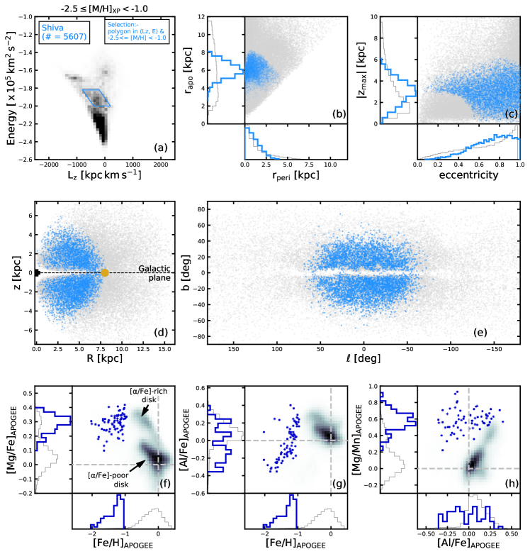
5 Characterization of Shiva
For characterizing the Shiva population, we follow the same approach as that described above for Shakti (in Section 4), except with slight modifications that are most suitable to study this substructure.
The selection of Shiva stars is again guided by the appearance of a prominent overdensity in panel of Fig. 3. Specifically, we restrict the full sample to the metallicity range and then retain only those stars that lie inside the polygon described by the four vertices: , , , ; the units are in []. This selection results in stars.
Fig. 5 shows the distribution of Shiva stars in the orbital space, spatial coordinates and the chemical space, and these distributions are quantified in Table 1. These stars orbit the Milky Way within the Galactocentric distance of (see distribution), with the amplitudes perpendicular to the Galactic plane ranging between and possess a moderately high range of eccentricities with . These stars are phase-mixed in the Galaxy (as shown in the and distributions).
Next, we find Shiva’s detailed chemical abundance properties in an analogous fashion to that of Shakti. In this case, with cross-matching of the Gaia-identified Shiva sample members with APOGEE, we find stars possessing [Fe/H], [Mg/Fe] and [Al/Fe] measurements, and of these, only stars possess [Mg/Mn] measurements. We find it is relatively metal–poor, with a median of [Fe/H], it is quite rich in Mg, Mn and Al, as listed in Table 1. Similarly to Shakti, Shiva’s population also has of stars with [Al/Fe] and shows a remarkably tight relation in [Fe/H] – [Al/Fe].
To compute Shiva’s stellar mass, if we base an estimate on the mass-metallicity relation of dwarf galaxies (Kirby et al., 2013), we arrive at : e.g., similar to the WLM known WLM dwarf galaxy, which has [Fe/H] and (Zhang et al., 2012; McConnachie, 2012). On the other hand, if we count the Shiva member stars and correct them for (orbital) angle incompleteness and the sample’s luminosity cut, we find , somewhat comparable to that of the POH substructure (Rix et al., 2022) whose stars are distributed in the inner of the Galaxy and they possess [M/H].
6 On the ”Nature” and origin of Shakti and Shiva
As we show below, Shakti and Shiva populations possess quite unconventional, intriguing properties that have not been observed previously in any substructure. This renders it quite challenging to understand the true nature and origin of these substructures. Below, we list down their properties and simultaneously interpret them to understand which of the following origin scenarios they possibly favour – (a) in-situ/disk origin (i.e., corresponding to the metal–rich disk population), (b) “proto-Galactic” origin (i.e., representing Aurora/POH–like metal–poor population, Belokurov & Kravtsov 2022; Rix et al. 2022), (c) dynamically “heated” disk origin (i.e., corresponding to the stars that were kicked out of the disk during an early collision with some massive merger, Bonaca et al. 2017; Di Matteo et al. 2019), (d) “spun up” halo population (i.e., representing those halo stars that got trapped in a ridge-like component in resonances with the Galactic bar, Dillamore et al. 2023) or (e) accreted origin (i.e., representing a population that was accreted inside a foreign galaxy, much like the GSE). The following discussion is summarised in Table 2.
| Possible origin | Shakti | Shiva |
| supporting properties: | ||
| in-situ/disk origin | High value of | |
| (i.e. a part of the | possesses stars with [Al/Fe], implying | |
| metal-rich disk | rapid enrichment inside a massive progenitor | |
| population) | ||
| seemingly inconsistent properties: | seemingly inconsistent properties: | |
| observed as a prominent blob in | location different than the disk | |
| [M/H] is well below the oldest/most | Too metal-poor to represent the disk population | |
| metal-poor part of the disk | ||
| orbits are not disk-like, but more halo-like | ||
| supporting properties: | Same arguments as for Shakti (on the left) | |
| “proto-Galactic” origin | [M/H]-poor | |
| (i.e., representing | chemical abundances similar to that of POH. | |
| Aurora/POH-like | possesses stars with [Al/Fe], implying | |
| metal-poor population) | rapid enrichment inside a massive progenitor | |
| seemingly inconsistent properties: | ||
| observed as a prominent blob in | ||
| higher binding energy () than Aurora/POH | ||
| supporting properties: | ||
| “Heated” disk origin | only slightly away from that of disk | |
| (i.e., a part of the disk | possesses stars with [Al/Fe], implying | |
| population that was kicked | rapid enrichment inside a massive progenitor | |
| out during an early | ||
| collision with a | seemingly inconsistent properties: | seemingly inconsistent properties: |
| massive merger) | observed as a prominent blob in | Too metal-poor to represent the disk population |
| [M/H] is well below the oldest/most | ||
| metal-poor part of the disk | ||
| supporting properties: | ||
| “Spun up” halo origin | location near the tip of | |
| (i.e., a part of the halo | Dillamore et al. (2023)’s ridge-like component | |
| population that got | ||
| trapped in a ridge-like | seemingly inconsistent properties: | seemingly inconsistent properties: |
| component in resonances | abundances are very distinct from GSE | Although prograde, but not near the |
| with the Galactic bar) | compact structure in the space, | location of Dillamore et al. (2023)’s primary ridge component |
| unlike Dillamore et al. (2023)’s extended ridge | abundances are very distinct from GSE | |
| located between | ||
| supporting properties: | Same argument as for Shakti (on the left) | |
| accreted origin | observed as high-contrast blob in | |
| (i.e., represents a | orbits are halo-like | |
| population that was | [M/H]-poor | |
| accreted inside a | ||
| foreign galaxy | seemingly inconsistent properties: | |
| enhanced in higher-order elements and | ||
| possesses stars with [Al/Fe], implying | ||
| rapid enrichment inside a massive progenitor |
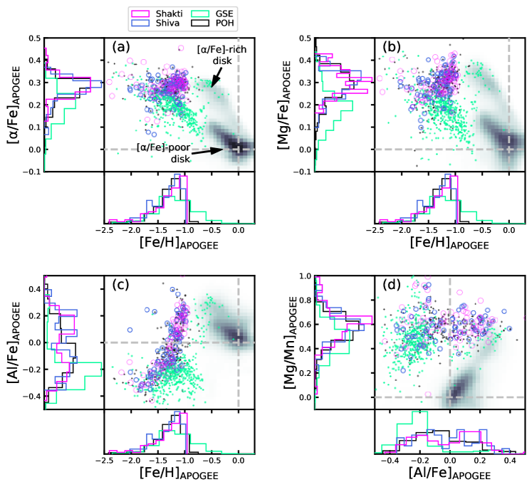
In doing so, we also require to compare the chemical abundances of Shakti and Shiva samples with those of GSE (which represents a prototypical massive merger) and POH. For this, we construct the GSE sample using our base data and follow Limberg et al. (2022)’s selection criteria: and . This renders a sample of stars. For POH, we follow Rix et al. (2022)’s recommendation: , and . This renders a sample of stars. These samples are cross-matched with the APOGEE dataset.
-
•
Both Shakti and Shiva populations are metal–poor, with their [Fe/H] well below the oldest/most-metal-poor part of the disk (, Mackereth et al. 2019). Secondly, they are enhanced in [Fe], [Al/Fe] and [Mg/Mn], with a median [Al/Fe] and of stars possessing [Al/Fe]. These chemical properties are shown in Fig. 6 and are interesting for the following reasons.
First, accreted metal–poor stars (with [Fe/H]) are presumed to stem from mergers that are less massive and less dense than the Milky Way (e.g., Helmi 2020). Consequently, such accreted stars should show chemical signatures of slower enrichment inside the low–mass progenitors (Wyse, 2016; Hawkins et al., 2015), which is reflected in their low [Al/Fe] () and with practically all the stars possessing [Al/Fe]. This latter point is based on Hasselquist et al. (2021) who analysed the five most massive dwarf galaxies accreted by the Milky Way – LMC, SMC, Sagittarius, Fornax and GSE; also see Horta et al. (2022).
Second, metal-poor stars whose [Fe], [Al/Fe] and [Mg/Mn] abundances point towards rapid enrichment, most likely would have happened within a massive and dense progenitor. Recently, Belokurov & Kravtsov (2022) analysed the APOGEE DR17 dataset, and dubbed the entire population of metal–poor ([Fe/H]) and Al–rich ([Al/Fe]) stars as Aurora, attributing them to correspond to the Milky Way pre-disk in-situ population that initially surrounded the Milky Way in a kinematically hot spheroidal configuration (and some of which later settled into the disk configuration, Sestito et al. 2020), but at the present-day is sparsely distributed within the solar radius. This population may overlap with the POH identified by Rix et al. (2022) as a dense central concentration of metal-poor, -enhanced stars. Rix et al. (2022) suggest that these stars need not come from a single in-situ progenitor, but may come from a few distinct dense and massive progenitors that coalesced at high-redshift ( ago) to form the proto-Galaxy.
To examine whether Shakti’s and Shiva’s abundance patterns look similar to the accreted–GSE or to Aurora/POH we perform Kolmogorov-Smirnov (KS) test for the null hypothesis that the given two samples are drawn from the same distribution. Shakti and Shiva samples are statistically very similar to that of POH, but very different than that of GSE (the null hypothesis can be rejected at level). Furthermore, these two substructures are even more enhanced in higher–order elements than LMC and SMC (for instance, compare our Fig. 6 with Figure 5 of Hasselquist et al. 2021). Moreover, the abundances of Shakti and Shiva are also very similar to each other, suggesting a similar progenitor or formation history.
In sum, the fact that Shakti and Shiva are [Fe/H]–poor but show abundance patterns indicative of rapid enrichment, similar to Aurora/POH, favours a “proto-Galactic” origin. Perhaps Shakti and Shiva were very early distinct entities that were simply more rapidly enriched than GSE (and also than LMC and SMC), perhaps they were more dense; at least at the time of accretion.
-
•
Both Shakti and Shiva populations are observed as high-contrast, tightly-bound overdensities in the space. Furthermore, both possess prograde motion, with Shakti possessing a much higher value (similar to that of the disk at the given ) and Shiva possessing a lower value. Moreover, they are more tightly bound in the Milky Way potential () than GSE but less tighly bound that the POH. These properties can be seen in Fig. 3.
Observations of such prominent overdensities in the space have conventionally been considered unambiguous telltale signs of accreted populations (e.g., Helmi et al. 2018; Naidu et al. 2020; Yuan et al. 2020), that were once born in a potential well that was distinct from the (current) Milky Way.
While Shakti’s high angular momentum makes it tempting to connect it with the in-situ/disk origin, this scenario seems implausible given its [Fe/H]. Secondly, while its location is similar to that of Dillamore et al. (2023)’s ridge–like component, its compact “blob”-like appearance in space argues against them being a ridge of former halo stars that became trapped in resonances with the Galactic bar. The feature that Dillamore et al. (2023) identified had a lower contrast than Shakti. If Shakti were part of a resonance-driven ridge in orbit space, we would expect the chemical properties to be similar to that of the halo stars, in particular to GSE (because the majority of halo stars presumably originated from GSE alone, Helmi 2020). But Shakti is chemically different from GSE, as shown by the abundance data. Furthermore, we note that Shakti’s location in orbit space is broadly similar to a postulated “metal–poor disk” (e.g., Carollo et al. 2019; Naidu et al. 2020). However, this feature is much more extended and of low contrast than Shakti.
If Shakti and Shiva were once distinct protogalactic fragments, they must have been incorporated ago; at least their star formation must have preceded the oldest and most metal-poor part of the disk (Xiang & Rix, 2022). This is qualitatively supported by the idea of taking the binding energy () as a proxy for the accretion time, which places them between the POH (, Rix et al. 2022) and GSE (, Belokurov et al. 2018; Helmi et al. 2018).
-
•
Both Shakti and Shiva populations are distributed within of the Milky Way, appear phase-mixed, and possess moderately large and eccentricity values. These properties can be seen in Figures 4 and 5. This indicates that the stars lie on dynamically hot orbits, hotter than the oldest part of the (-enhanced) disk. This may be consistent with both the accreted and the “heated” disk scenarios. However, the latter scenario seems unlikely, given that Shakti and Shiva are observed as high–contrast orbit–substructures (and not sparse distribution of stars, such as that observed in the Splash substructure). Even their [M/H]–deficiency opposes any plausible connection with the disk.
In view of the above discussion, the following scenario appears most consistent with the totality of the observational evidence: Shakti and Shiva represent two of those early, massive progenitors that coalseced at high redshift (perhaps ago), perhaps the last event form the proto-Galaxy, before disk formation commenced. These progenitors enriched more rapidly, and were likely even more dense and massive than GSE (and also LMC and SMC), at least back then at the time of accretion. This conjecture is supported by the combination of their unconventional properties.
To conclude the discussion, we ask whether Shakti and Shiva have any population of globular clusters dynamically “associated” with them? This is an interesting question because recent studies have shown that it is common for massive mergers to bring in populations of such objects (e.g., Massari et al. 2019; Myeong et al. 2019; Malhan et al. 2022). To this end, it seems reasonable to link those Milky Way globular clusters that possess orbits and metallicities similar to these substructures. For the globular clusters, we obtain their orbits and metallicities from Malhan et al. (2022) and Harris (2010), respectively. Next, we consider only those globular clusters that lie within the same polygon and [M/H] range as that described to select the substructure stars. Shakti is found to be linked with only cluster (namely, NGC 6235) and Shiva with clusters (namely, NGC 5986, NGC 6121/M 4, NGC 6218/M 12, NGC 6287, NGC 6333/M 9, NGC 6397,NGC 6809/M 55).
7 Conclusion and Discussion
We have identified two new stellar structures in the Milky Way, seen as prominent, confined overdensities in the distribution of bright (), metal–poor () stars. This was enabled by using the novel XGBoost dataset (Rix et al., 2022; Andrae et al., 2023) that provides robust and precise metallicity estimates (based on Gaia DR3’s BP/RP spectra) that can be combined with 6D phase-space measurements (from Gaia DR3 itself) for millions of stars; practically for the highest number of stars ever. More detailed chemical abundance patterns were enabled by SDSS DR17.
Shakti and Shiva populations possess an unconventional combination of orbital and abundance properties that have not been observed previously. This is because it has become possible only recently to combine Gaia and SDSS DR17 datasets to disentangle different Galactic populations (e.g., based on the stellar orbits, [M/H] and [Al/Fe]), even in the inner Galaxy and at old ages, plausibly unearthing ancient ( old) populations that formed the proto–Galaxy (Belokurov & Kravtsov, 2022; Rix et al., 2022). There may be a preponderance of observational clues that argue for Shakti and Shiva representing two of early, massive () – or at least dense – fragments that coalesced at high redshifts (perhaps or ago) to form the proto–Galaxy. They are less tightly bound than Aurora/POH and therefore have a better chance of appearing as distinct overdensities in orbit-space.
However, there are important aspects in which Shakti and Shiva match expectations for ancient stars that gradually picked up angular momentum by resonant orbit trapping caused by the Galactic bar; a scenario proposed recently by (Dillamore et al., 2023). This scenario predicts ridges in the plane towards the prograde direction. And for the observationally inferred bar speed, these ridges should lie at orbital frequencies (or binding energies ) broadly similar to those of Shakti and ShivaṠuch orbital trapping should affect stars of all metallicities, and we see a fairly broad metallicity distribution in both substructures. However, quantitatively, this scenario does not match our observations: Shakti’s compact distribution in does not at all look like an extended ridge as observed in the Dillamore et al. (2023) study. Nor does it explain the abundance pattern mismatch between Shakti and GSE, which is the presumed low- precursor in this scenario. Whether these inconsistencies, which argue against a spun-up-by-bar scenario, can be reconciled remains to be seen.
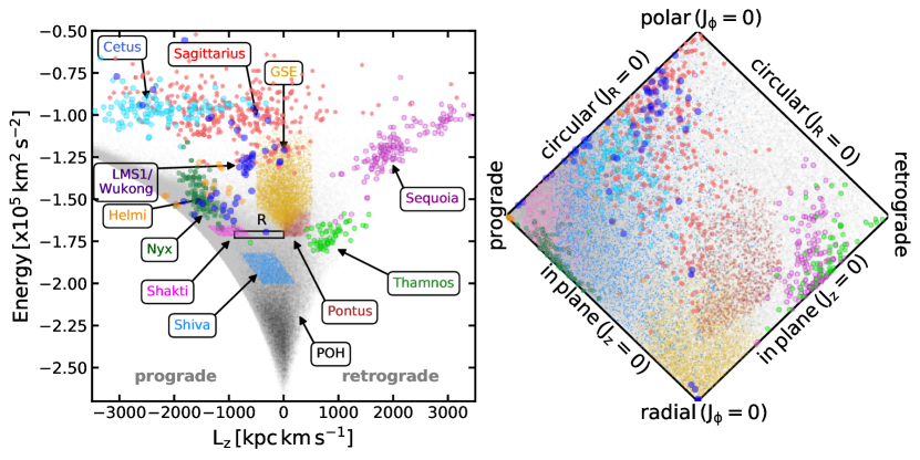
In closing, we put Shakti and Shiva in the dynamical context of the various other sub structures detected in the past. Fig. 7 shows different substructures of the Milky Way444The member stars of these different populations are obtained as follows. The Sagittarius stars are taken from Ibata et al. (2020), the Cetus population from Yuan et al. (2022), LMS-1/Wukong from Malhan et al. (2021), Nyx from Necib et al. (2020); Wang et al. (2022), Helmi stream stars from Koppelman et al. (2019b), Pontus from Malhan (2022), Thamnos and Sequoia from Koppelman et al. (2019a). For POH we follow Rix et al. (2022)’s recommendation and select stars with , and ., most of which have been discovered using the Gaia dataset, and their detailed chemical abundances are generally studied using the SDSS, LAMOST or GALAH surveys. Excitingly, Gaia’s excellent all–sky 5D astrometry and metallicities are now being complemented by SDSS-V (Kollmeier et al., 2017), in particular also for Shakti and Shiva. In the near future, these spectroscopic efforts will be complemented by measurements from the upcoming WEAVE (Dalton et al., 2014) and 4MOST (de Jong et al., 2019) surveys that will map the northern and southern hemispheres, respectively. Furthermore, observations by the Rubin Observatory (fka LSST, Ivezić et al. 2019) will eventually provide a means to determine precise distances of the halo stars. These surveys together will provide 6D phase–space measurements and abundances of stars out to , thereby allowing us to create a high–resolution chemo–dynamical map of different Galactic populations, giving us once in a lifetime opportunity to unravel the complete formation history of our Galaxy.
Acknowledgements
We thank the referee for helpful comments and sug- gestions. We also thank Vasily A. Belokurov for enlightening and stimulating discussions on the topic.
This work has made use of data from the European Space Agency (ESA) mission Gaia (https://www.cosmos.esa.int/gaia), processed by the Gaia Data Processing and Analysis Consortium (DPAC, https://www.cosmos.esa.int/web/gaia/dpac/consortium). Funding for the DPAC has been provided by national institutions, in particular the institutions participating in the Gaia Multilateral Agreement.
Funding for the Sloan Digital Sky Surveys IV and V has been provided by the Alfred P. Sloan Foundation, the Heising-Simons Foundation, the National Science Foundation, and the Participating Institutions. SDSS acknowledges support and resources from the Center for High-Performance Computing at the University of Utah. The SDSS web site is www.sdss.org.
SDSS is managed by the Astrophysical Research Consortium for the Participating Institutions of the SDSS Collaboration, including the Carnegie Institution for Science, Chilean National Time Allocation Committee (CNTAC) ratified researchers, the Gotham Participation Group, Harvard University, Heidelberg University, The Johns Hopkins University, L’Ecole polytechnique fédérale de Lausanne (EPFL), Leibniz-Institut für Astrophysik Potsdam (AIP), Max-Planck-Institut für Astronomie (MPIA Heidelberg), Max-Planck-Institut für Extraterrestrische Physik (MPE), Nanjing University, National Astronomical Observatories of China (NAOC), New Mexico State University, The Ohio State University, Pennsylvania State University, Smithsonian Astrophysical Observatory, Space Telescope Science Institute (STScI), the Stellar Astrophysics Participation Group, Universidad Nacional Autónoma de México, University of Arizona, University of Colorado Boulder, University of Illinois at Urbana-Champaign, University of Toronto, University of Utah, University of Virginia, Yale University, and Yunnan University.
Appendix A Computing stellar mass of a phase-mixed population
To compute the stellar mass of Shakti and Shiva, we use the following idea. We can simply count the member stars, accounting for the fact that we only possess giant stars in our sample (and the lower luminosity stars are missing) and that we observe member stars in a specific range of orbital phases (and not at all the phases). The latter occurs because Gaia (much like any other Galactic survey) fails to observe stars at greater distances beyond the solar neighbourhood, and also in the Galactic disk region due to the dust extinction (as can be seen from Fig. 2). In this regard, we note that Frankel et al. (2023) suggests that for phase-mixed substructures (such as Shakti and Shiva), the distribution in all three orbital angles is expected to be uniform. If we can estimate the ”incompleteness” factor in the angle space, then we can estimate substructure’s total stellar mass, via
| (A1) | ||||
Here, is the number of (giant star) sample members that we attribute to the substructure (shown in Figures 4a and 5a), is the factor accounting for the sample incompleteness and “” is the stellar population mass per giant star (at a given absolute magnitude ). It is this parameter whose estimate relies on the above assumption. “” is the stellar population mass per giant star (at the absolute magnitude ). Below, we detail our procedure to compute the stellar mass.
A.1 Shakti
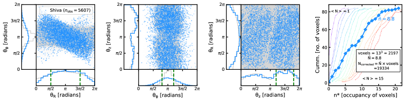
First, we compute the parameter . The fact that the sample is incomplete can be realised from Fig. 8 which shows that the distribution of stars in the space is not uniform. This is because we can only observe giant stars in our quadrant of the Galaxy. However, based on our above assumption for a phase-mixed population, the expectation is that this distribution would have been uniform, had we been able to observe all the Shakti stars in the entire Galaxy. Therefore, we require to estimate the mean occupation number , which is the average number of stars in a given voxel. For this, we manually select the sub-space where the distribution appears to be most complete (as shown in Fig. 8): , , and set the voxel bin size as radians. The resulting cumulative distribution of Shakti stars is shown in Fig. 8. Upon comparing this curve with the Poisson curves, we find the average stellar occupancy in a given voxel as . This value needs to be multiplied with the total number of voxels, i.e., , which gives the total number of stars after correcting for sample incompleteness as . This implies .
Second, we compute the parameter “” following the same approach described in Rix et al. (2022). For this, we use the globular cluster NGC 362, which serves as a template for an old, [M/H] population. Beyond NGC 362’s half-mass radius of (Baumgardt & Hilker, 2018), we find about giants with (this magnitude limit is set by the faint limit of the Shakti stars after the above sub-space selection). Given NGC 362’s total mass of (Baumgardt & Hilker, 2018), this implies one giant (at ) per of the total stellar population mass.
Finally, the above and values are substituted in equation A1 to obtain the stellar mass as .
A.2 Shiva
To compute Shiva’s stellar mass, we follow the same procedure as above, but with slight modifications that are most suited for this stellar population. These include changes in the range of , where we find Shiva’s distribution to be most complete: , , . In this case, we find , which in turn gives . This implies . Next, “” is computed similarly as above using NGC 362. In this way, we estimate for Shiva .
References
- Abdurro’uf et al. (2021) Abdurro’uf, Accetta, K., Aerts, C., et al. 2021, arXiv e-prints, arXiv:2112.02026. https://arxiv.org/abs/2112.02026
- Almeida et al. (2023) Almeida, A., Anderson, S. F., Argudo-Fernández, M., et al. 2023, arXiv e-prints, arXiv:2301.07688, doi: 10.48550/arXiv.2301.07688
- Andrae et al. (2023) Andrae, R., Rix, H.-W., & Chandra, V. 2023, arXiv e-prints, arXiv:2302.02611, doi: 10.48550/arXiv.2302.02611
- Arenou et al. (2018) Arenou, F., Luri, X., Babusiaux, C., et al. 2018, A&A, 616, A17, doi: 10.1051/0004-6361/201833234
- Baumgardt & Hilker (2018) Baumgardt, H., & Hilker, M. 2018, MNRAS, 478, 1520, doi: 10.1093/mnras/sty1057
- Bell et al. (2008) Bell, E. F., Zucker, D. B., Belokurov, V., et al. 2008, ApJ, 680, 295, doi: 10.1086/588032
- Belokurov et al. (2018) Belokurov, V., Erkal, D., Evans, N. W., Koposov, S. E., & Deason, A. J. 2018, MNRAS, 478, 611, doi: 10.1093/mnras/sty982
- Belokurov & Kravtsov (2022) Belokurov, V., & Kravtsov, A. 2022, MNRAS, 514, 689, doi: 10.1093/mnras/stac1267
- Belokurov et al. (2020) Belokurov, V., Sanders, J. L., Fattahi, A., et al. 2020, MNRAS, 494, 3880, doi: 10.1093/mnras/staa876
- Bensby et al. (2014) Bensby, T., Feltzing, S., & Oey, M. S. 2014, A&A, 562, A71, doi: 10.1051/0004-6361/201322631
- Birnboim & Dekel (2003) Birnboim, Y., & Dekel, A. 2003, MNRAS, 345, 349, doi: 10.1046/j.1365-8711.2003.06955.x
- Bland-Hawthorn & Gerhard (2016) Bland-Hawthorn, J., & Gerhard, O. 2016, ARA&A, 54, 529, doi: 10.1146/annurev-astro-081915-023441
- Blitz & Spergel (1991) Blitz, L., & Spergel, D. N. 1991, ApJ, 379, 631, doi: 10.1086/170535
- Bonaca et al. (2017) Bonaca, A., Conroy, C., Wetzel, A., Hopkins, P. F., & Kereš, D. 2017, ApJ, 845, 101, doi: 10.3847/1538-4357/aa7d0c
- Bovy (2015) Bovy, J. 2015, ApJS, 216, 29, doi: 10.1088/0067-0049/216/2/29
- Bovy et al. (2012) Bovy, J., Rix, H.-W., & Hogg, D. W. 2012, ApJ, 751, 131, doi: 10.1088/0004-637X/751/2/131
- Bressan et al. (2012) Bressan, A., Marigo, P., Girardi, L., et al. 2012, MNRAS, 427, 127, doi: 10.1111/j.1365-2966.2012.21948.x
- Buder et al. (2021) Buder, S., Sharma, S., Kos, J., et al. 2021, MNRAS, 506, 150, doi: 10.1093/mnras/stab1242
- Carollo et al. (2019) Carollo, D., Chiba, M., Ishigaki, M., et al. 2019, The Astrophysical Journal, 887, 22, doi: 10.3847/1538-4357/ab517c
- Conroy et al. (2022) Conroy, C., Weinberg, D. H., Naidu, R. P., et al. 2022, arXiv e-prints, arXiv:2204.02989, doi: 10.48550/arXiv.2204.02989
- Dalton et al. (2014) Dalton, G., Trager, S., Abrams, D. C., et al. 2014, in Society of Photo-Optical Instrumentation Engineers (SPIE) Conference Series, Vol. 9147, Ground-based and Airborne Instrumentation for Astronomy V, ed. S. K. Ramsay, I. S. McLean, & H. Takami, 91470L, doi: 10.1117/12.2055132
- de Jong et al. (2019) de Jong, R. S., Agertz, O., Berbel, A. A., et al. 2019, The Messenger, 175, 3, doi: 10.18727/0722-6691/5117
- Di Matteo et al. (2019) Di Matteo, P., Haywood, M., Lehnert, M. D., et al. 2019, A&A, 632, A4, doi: 10.1051/0004-6361/201834929
- Dillamore et al. (2023) Dillamore, A. M., Belokurov, V., Evans, N. W., & Davies, E. Y. 2023, arXiv e-prints, arXiv:2303.00008, doi: 10.48550/arXiv.2303.00008
- Drimmel & Poggio (2018) Drimmel, R., & Poggio, E. 2018, Research Notes of the AAS, 2, 210, doi: 10.3847/2515-5172/aaef8b
- Frankel et al. (2023) Frankel, N., Bovy, J., Tremaine, S., & Hogg, D. W. 2023, MNRAS, 521, 5917, doi: 10.1093/mnras/stad908
- Gravity Collaboration et al. (2018) Gravity Collaboration, Abuter, R., Amorim, A., et al. 2018, A&A, 615, L15, doi: 10.1051/0004-6361/201833718
- Harris (2010) Harris, W. E. 2010, arXiv e-prints, arXiv:1012.3224, doi: 10.48550/arXiv.1012.3224
- Hasselquist et al. (2021) Hasselquist, S., Hayes, C. R., Lian, J., et al. 2021, ApJ, 923, 172, doi: 10.3847/1538-4357/ac25f9
- Hawkins et al. (2015) Hawkins, K., Jofré, P., Masseron, T., & Gilmore, G. 2015, MNRAS, 453, 758, doi: 10.1093/mnras/stv1586
- Hawkins et al. (2016) Hawkins, K., Masseron, T., Jofré, P., et al. 2016, A&A, 594, A43, doi: 10.1051/0004-6361/201628812
- Helmi (2020) Helmi, A. 2020, ARA&A, 58, 205, doi: 10.1146/annurev-astro-032620-021917
- Helmi et al. (2018) Helmi, A., Babusiaux, C., Koppelman, H. H., et al. 2018, Nature, 563, 85, doi: 10.1038/s41586-018-0625-x
- Helmi et al. (1999) Helmi, A., White, S. D. M., de Zeeuw, P. T., & Zhao, H. 1999, Nature, 402, 53, doi: 10.1038/46980
- Horta et al. (2022) Horta, D., Schiavon, R. P., Mackereth, J. T., et al. 2022, MNRAS, doi: 10.1093/mnras/stac3179
- Ibata et al. (2020) Ibata, R., Bellazzini, M., Thomas, G., et al. 2020, ApJ, 891, L19, doi: 10.3847/2041-8213/ab77c7
- Ibata et al. (1994) Ibata, R. A., Gilmore, G., & Irwin, M. J. 1994, Nature, 370, 194, doi: 10.1038/370194a0
- Ivezić et al. (2019) Ivezić, Ž., Kahn, S. M., Tyson, J. A., et al. 2019, ApJ, 873, 111, doi: 10.3847/1538-4357/ab042c
- Kirby et al. (2013) Kirby, E. N., Cohen, J. G., Guhathakurta, P., et al. 2013, ApJ, 779, 102, doi: 10.1088/0004-637X/779/2/102
- Kollmeier et al. (2017) Kollmeier, J. A., Zasowski, G., Rix, H.-W., et al. 2017, arXiv e-prints, arXiv:1711.03234, doi: 10.48550/arXiv.1711.03234
- Koppelman et al. (2019a) Koppelman, H. H., Helmi, A., Massari, D., Price-Whelan, A. M., & Starkenburg, T. K. 2019a, A&A, 631, L9, doi: 10.1051/0004-6361/201936738
- Koppelman et al. (2019b) Koppelman, H. H., Helmi, A., Massari, D., Roelenga, S., & Bastian, U. 2019b, A&A, 625, A5, doi: 10.1051/0004-6361/201834769
- Kruijssen et al. (2019) Kruijssen, J. M. D., Pfeffer, J. L., Reina-Campos, M., Crain, R. A., & Bastian, N. 2019, MNRAS, 486, 3180, doi: 10.1093/mnras/sty1609
- Limberg et al. (2022) Limberg, G., Souza, S. O., Pérez-Villegas, A., et al. 2022, The Astrophysical Journal, 935, 109, doi: 10.3847/1538-4357/ac8159
- Lindegren et al. (2021) Lindegren, L., Klioner, S. A., Hernández, J., et al. 2021, A&A, 649, A2, doi: 10.1051/0004-6361/202039709
- Ma et al. (2016) Ma, X., Hopkins, P. F., Faucher-Giguère, C.-A., et al. 2016, MNRAS, 456, 2140, doi: 10.1093/mnras/stv2659
- Mackereth et al. (2019) Mackereth, J. T., Schiavon, R. P., Pfeffer, J., et al. 2019, MNRAS, 482, 3426, doi: 10.1093/mnras/sty2955
- Malhan (2022) Malhan, K. 2022, ApJ, 930, L9, doi: 10.3847/2041-8213/ac67da
- Malhan et al. (2021) Malhan, K., Yuan, Z., Ibata, R. A., et al. 2021, ApJ, 920, 51, doi: 10.3847/1538-4357/ac1675
- Malhan et al. (2022) Malhan, K., Ibata, R. A., Sharma, S., et al. 2022, ApJ, 926, 107, doi: 10.3847/1538-4357/ac4d2a
- Massari et al. (2019) Massari, D., Koppelman, H. H., & Helmi, A. 2019, A&A, 630, L4, doi: 10.1051/0004-6361/201936135
- McConnachie (2012) McConnachie, A. W. 2012, AJ, 144, 4, doi: 10.1088/0004-6256/144/1/4
- McMillan (2017) McMillan, P. J. 2017, MNRAS, 465, 76, doi: 10.1093/mnras/stw2759
- Myeong et al. (2019) Myeong, G. C., Vasiliev, E., Iorio, G., Evans, N. W., & Belokurov, V. 2019, MNRAS, 488, 1235, doi: 10.1093/mnras/stz1770
- Naidu et al. (2020) Naidu, R. P., Conroy, C., Bonaca, A., et al. 2020, ApJ, 901, 48, doi: 10.3847/1538-4357/abaef4
- Necib et al. (2020) Necib, L., Ostdiek, B., Lisanti, M., et al. 2020, Nature Astronomy, 4, 1078, doi: 10.1038/s41550-020-1131-2
- Ness et al. (2013) Ness, M., Freeman, K., Athanassoula, E., et al. 2013, MNRAS, 430, 836, doi: 10.1093/mnras/sts629
- Newberg et al. (2009) Newberg, H. J., Yanny, B., & Willett, B. A. 2009, ApJ, 700, L61, doi: 10.1088/0004-637X/700/2/L61
- Pedregosa et al. (2011) Pedregosa, F., Varoquaux, G., Gramfort, A., et al. 2011, Journal of Machine Learning Research, 12, 2825, doi: 10.48550/arXiv.1201.0490
- Recio-Blanco et al. (2023) Recio-Blanco, A., de Laverny, P., Palicio, P. A., et al. 2023, A&A, 674, A29, doi: 10.1051/0004-6361/202243750
- Renaud et al. (2021) Renaud, F., Agertz, O., Read, J. I., et al. 2021, MNRAS, 503, 5846, doi: 10.1093/mnras/stab250
- Rix & Bovy (2013) Rix, H.-W., & Bovy, J. 2013, A&A Rev., 21, 61, doi: 10.1007/s00159-013-0061-8
- Rix et al. (2022) Rix, H.-W., Chandra, V., Andrae, R., et al. 2022, ApJ, 941, 45, doi: 10.3847/1538-4357/ac9e01
- Schlegel et al. (1998) Schlegel, D. J., Finkbeiner, D. P., & Davis, M. 1998, ApJ, 500, 525, doi: 10.1086/305772
- Sestito et al. (2020) Sestito, F., Martin, N. F., Starkenburg, E., et al. 2020, MNRAS, 497, L7, doi: 10.1093/mnrasl/slaa022
- Sharma & Johnston (2009) Sharma, S., & Johnston, K. V. 2009, ApJ, 703, 1061, doi: 10.1088/0004-637X/703/1/1061
- Stern et al. (2021) Stern, J., Faucher-Giguère, C.-A., Fielding, D., et al. 2021, ApJ, 911, 88, doi: 10.3847/1538-4357/abd776
- Tenachi et al. (2022) Tenachi, W., Oria, P.-A., Ibata, R., et al. 2022, ApJ, 935, L22, doi: 10.3847/2041-8213/ac874f
- Wang et al. (2022) Wang, S., Necib, L., Ji, A. P., et al. 2022, arXiv e-prints, arXiv:2210.15013, doi: 10.48550/arXiv.2210.15013
- Wyse (2016) Wyse, R. F. G. 2016, in Astronomical Society of the Pacific Conference Series, Vol. 507, Multi-Object Spectroscopy in the Next Decade: Big Questions, Large Surveys, and Wide Fields, ed. I. Skillen, M. Balcells, & S. Trager, 13
- Xiang & Rix (2022) Xiang, M., & Rix, H.-W. 2022, Nature, 603, 599, doi: 10.1038/s41586-022-04496-5
- Yanny et al. (2009) Yanny, B., Rockosi, C., Newberg, H. J., et al. 2009, AJ, 137, 4377, doi: 10.1088/0004-6256/137/5/4377
- Yuan et al. (2020) Yuan, Z., Chang, J., Beers, T. C., & Huang, Y. 2020, ApJ, 898, L37, doi: 10.3847/2041-8213/aba49f
- Yuan et al. (2022) Yuan, Z., Malhan, K., Sestito, F., et al. 2022, The Astrophysical Journal, 930, 103, doi: 10.3847/1538-4357/ac616f
- Zahid et al. (2014) Zahid, H. J., Dima, G. I., Kudritzki, R.-P., et al. 2014, ApJ, 791, 130, doi: 10.1088/0004-637X/791/2/130
- Zhang et al. (2012) Zhang, H.-X., Hunter, D. A., Elmegreen, B. G., Gao, Y., & Schruba, A. 2012, AJ, 143, 47, doi: 10.1088/0004-6256/143/2/47
- Zhao et al. (2012) Zhao, G., Zhao, Y.-H., Chu, Y.-Q., Jing, Y.-P., & Deng, L.-C. 2012, Research in Astronomy and Astrophysics, 12, 723, doi: 10.1088/1674-4527/12/7/002