Dynamical systems analysis of a cosmological model with interacting Umami Chaplygin fluid in adiabatic particle creation mechanism: Some bouncing features

Abstract

The present work aims to investigate an interacting Umami Chaplygin gas in the background dynamics of spatially flat Friedmann-Lemaitre-Robertson-Walker (FLRW) universe when adiabatic particle creation is allowed. Here, the universe is taken to be an open thermodynamical model where the particle is created irreversibly and consequently, the creation pressure comes into the energy-momentum tensor of the material content. The rate at which particle created is assumed to have a linear relation with Hubble parameter and the created particle is dark matter (pressureless). The Umami Chaplygin gas is considered as dark energy while pressureless dust is taken as dark matter and a phenomenological interaction term is taken for mathematical simplicity. Dynamical analysis is performed to obtain an overall evolution of the model we consider. The autonomous system is obtained by considering dimensionless variables in terms of cosmological variables.The nature of critical points of the autonomous system is analyzed by perturbing the system around the critical points. Classical stability of the model is also performed at each critical points. This study explores some cosmologically viable scenarios when we constrain the model parameters. Some critical points exhibit the accelerated de Sitter expansion of the universe at both the early phase as well as the late phase of evolution which is characterized by completely Umami Chaplygin fluid equation of state. Scaling solutions are also described by some other critical points showing late-time accelerated attractors in phase space satisfying present observational data, and solving the coincidence problem. In a specific region of parameters, a sequence of critical points is achieved exhibiting a unified cosmic evolution of the universe starting from early inflation (represented by source point), which is followed by an decelerated intermediate (described by saddle solution) phase, and finally go through the late-time dark energy dominated universe (represented by stable point). Finally, non-singular bouncing behavior of the universe is also investigated for this model numerically.

I Introduction

One of the main crucial issues in modern cosmology is the present acceleration of the universe which is favored by numerous observational data obtained from Supernovae Type Ia (SNe Ia) [1, 2], Cosmic Microwave Background Radiation (CMBR) [3], the Baryon Acoustic Oscillations (BAOs) [4], Plank data [5, 6] etc. Cosmologists have addressed these in theory by introducing a new matter source in the energy-momentum tensor in the Einstein Field Equation. The matter source is dubbed as Dark Energy (DE), and being an exotic type fluid having a huge negative pressure, it has significant role in making gravitational repulsive effect which is responsible for acceleration. Although, the DE can successfully explain the present acceleration of the universe, the nature of the DE is completely unknown to us. Also, it violates the strong energy condition (i.e., $\rho+3p<0$) and the equation of state satisfies $\omega=\frac{p}{\rho}<-\frac{1}{3}$. In this context, the most preferred candidate for the DE is ‘cosmological constant’ ($\Lambda$) which has constant equation of state ($\omega_{\Lambda}=-1$). The cosmological constant along with cold dark matter constitutes the $\Lambda$CDM model [7, 8, 9] providing the best fitted result to the observational data. However, the model has two serious theoretical issues: one is the ‘cosmological constant problem’ arising due to the disagreement between observed small value and the theoretical large value of vacuum predicted by the quantum field theory. Another is the ‘cosmic coincidence problem’ which refers to as ‘why the energy densities of two dark fluids are of the same order today, though they scale differently in their cosmic evolution?’. Motivated from this, people are looking for new cosmological models which are free from the above two problems.
Since then, several models based on perfect fluid equation of state have been introduced to address such problems. A new model in this context, having perfect fluid equation of state turns out to be very promising. This equation of state is expected to satisfy two limits which follow the expansion rate at high redshift as well as at low redshift. That is, this type of fluid mimics the matter(dust) dominated epoch at early stage of evolution of the universe and an accelerated expansion phase at late-times. This class of models belongs to the Chaplygin gas type fluid. The Chaplygin gas models are popular in cosmology due to the fact that they can behave unified description of DE and DM within a single model. The original Chaplygin gas was first introduced by Kamenschik, Moschella, and Pasquier [10] and characterized by the following EoS:

$$p=-\frac{A}{\rho}$$

where $A$ is positive constant and this was introduced as an alternative to quintessence. After that a plenty generalizations have been reported in the literature (see for instance in Ref. [11]). One of such generalizations, known as Generalized Chaplygin gas (GCG) was introduced by Bento et. al.[12] with EoS:

$$p=-\frac{A}{\rho^{\alpha}}$$

where $\alpha$ is positive constant and $\alpha\in[0,~{}1]$. Latter, a modified Chaplygin gas (MCG) was also proposed with the equation of state

$$p=B\rho-\frac{A}{\rho^{\alpha}}$$

where $B$ is positive constant. For $B=0$ the EoS reduces to the generalized Chaplygin gas (GCG) EoS while for $B=0,~{}\alpha=1$, it recovers the original Chaplygin gas. Specifically, $A=0$ and $B=\frac{1}{3}$ indicate that the EoS leads to radiation dominated evolution. The modified Chaplygin gas and Generalized Chaplygin gas models have been extensively studied in the context of cosmology in the literature (see in Refs. [13]).
Recently, Lazkoz et al. [14] introduced a new modification in Chaplygin fluid described by the following EoS:

$$p=-\frac{\rho}{\frac{1}{|\omega|}+\frac{\rho^{2}}{|A|}}$$ (1)

where $\rho$ is the energy density and $p$ is the pressure of the fluid. $A$ and $\omega$ are the real constants. The fluid can describe different phases of evolution depending on restrictions on parameters $A$ and $\omega$. In particular, at high energy limit, the fluid mimics as $p\longrightarrow-\frac{|A|}{\rho}$, which is obviously equivalent to the equation of state of usual Chaplygin gas. On the other hand, at the low energy density limit one obtains $p\longrightarrow-|\omega|\rho$ which describes the negative effective equation of state. Unlike the other models (previously described) of Chaplygin fluid, the Umami Chaplygin gas describes not only unified model of DE and DM, but also can represent the unified description of dark fluid and baryonic matter [14]. That is the Umami Chaplygin fluid has a significant role in contributing the total matter distribution of the universe. Therefore, it is interesting to study the Umami Chaplygin gas as an alternative to $\Lambda$CDM. The Umami Chaplygin fluid has been studied further by Biswas and Biswas in Ref. [15] in the context of dynamical and thermodynamical point of view and many interesting results have been reported therein.
From the several astrophysical data it is speculated that the main material content of the universe is constituted by pressureless dark matter (DM) contributing $28\%$ and dark energy (DE) contributing around $68\%$ of the total energy budget of the universe. Hence, the dark sector is the dominant source, is almost $96\%$ of the universe [16]. Since, a very little is known about the nature of these two constituents, an interaction between them cannot be neglected. To address the coincidence problem, interacting dynamics in cosmology came into focus see in Refs. [17, 18, 19, 20, 21]. Since there is no as such guiding principle for choosing interaction term, the interaction term can be taken on purely phenomenological ground. Phenomenological interacting scenarios have been investigated in the literature (see for instance in Refs. [22, 23, 24, 25, 26, 37, 27, 28, 29, 30, 31, 32, 33, 34, 35, 36]). Recent studies indicate that introduction of an interaction in the dark sector can alleviate $H_{0}$ tension [38, 39, 40, 41, 65, 44, 42, 48, 43, 45, 46, 47, 49, 50, 51, 52, 53, 54, 55, 56, 57, 58, 59, 60, 61, 62, 63, 64] appearing due to disagreement between the CMB measurements by Planck satellite within $\Lambda CDM$ cosmology [16] and SH$0$ES [66] and $S_{8}$ tension [67, 68, 69, 70, 71] arising due to discordance (i.e. many sigmas gap) between the Planck and Weak Lensing measurements [72]. Beside these, it is noted that an interaction can be able to explain the phantom phase of the DE without any need of a scalar field with negative kinetic [73, 74, 75] . Therefore, recent research has a lot of interest to search for dynamics of interacting scenario in cosmology. In this context, a comprehensive study on interacting dark energy models is required and for that one may follow two works [22, 27] already in the literature.

In view of cosmological study, particle creation mechanism can be a viable alternative in addressing the cosmic acceleration. Many studies stress on the fact that the particle creation model can closely mimic as $\Lambda$CDM cosmology[76, 77, 78, 79, 80, 37]. In this model, the concept is that the matter is created from time-varying gravitational field mimicking as cold dark matter [81, 82, 83, 84, 85, 86, 87, 88]. A microscopic description of matter creation was first discovered in 1939 by Schrodinger himself (see in Ref. [89]). After that Parker and collaborators [90] extended the investigations in curved space-time on the background of quantum field theory. Further, Prigogine et al [81, 82] investigated matter creation mechanism in view of macroscopic universe. They applied the concept in cosmological study by assuming the universe as an open, non-equilibrium thermodynamical model. Since then, people have investigated successfully this particle creation mechanism in context of cosmology. Thus, one may observe, in this context that the dissipative phenomenon in flat FLRW model may arise in form of bulk viscous pressure due to non-conservation of particle numbers, i.e., $N^{\mu}_{;\mu}\neq 0$. As a result, the balance equation for particle number density will get modified unlike the usual balance equation. In the present work, we choose FLRW geometry where the universe is considered as an open thermodynamical system and the non-conservation of particle gets modified as the following equation:

$$N^{\mu}_{;\mu}=\dot{n}+\Theta n=n\Gamma,$$ (2)

where $\Gamma$ is the rate of change of particle number and $n$ is the particle number density defined by $n=\frac{N}{V}$, where $V=a^{3}$ is the co-moving volume. The particle flow vector is referred to as $N^{\mu}=nu^{\mu}$, $u$ is the four-velocity vector related to the expansion of congruence of time-like geodesic by the relation $\Theta=u^{\mu}_{;\mu}$. It is to be mentioned that for FLRW universe, one may obtain $\Theta=u^{\mu}_{;\mu}=3H$ and $\dot{n}=n_{\mu}u^{\mu}$ and the thermodynamics of matter creation will be discussed in next section.

It is to be noted that there is no guiding principle to choose the creation rate $\Gamma$, but the positive value of the $\Gamma$ is reassuring for the sake of validity of the second law of thermodynamics. Recent studies regarding cosmic evolution of FLRW universe in the context of adiabatic matter creation have gained a great interest. The present acceleration of evolution in this context has been studied in Refs. [91, 92, 37, 93]. At the same time, future deceleration of the evolution is also realized in Refs. [91, 94]. It is interesting to note that an early inflationary scenario has been found in the context of particle creation model [95]. Further, an emergent scenario is obtained in Refs. [96, 97] and subsequently, a complete cosmic evolution is found in Ref. [98]. The authors in Ref. [99], investigated the FLRW cosmology in the framework of adiabatic matter creation mechanism and found cosmological solution from early big-bang to late-time de Sitter. They also proposed a bounce universe in the context of Loop Quantum Cosmology (LQC) from the dynamical perspective. Then, in Ref. [65] the early time acceleration as well as the late-time acceleration of the universe are studied. Moreover, a phantom crossing behavior is also obtained in Ref. [92, 37] without considering the phantom fields in cosmological dynamics. In a recent work (see in Ref. [100]), the authors investigated different scenarios of cosmic evolution by considering Holographic dark energy in the context of particle creation where they made different phenomenological choices of creation rate in terms of Hubble function. A dynamical systems analysis is also carried out in Ref. [101] for several interacting dark energy in the framework of particle creation mechanism, where creation rate $\Gamma$ is taken as linear function of Hubble parameter. A new cosmological model, called Created Cold Dark Matter (CCDM) scenario is proposed in literature [76, 77, 88] via particle creation mechanism. This can be a viable alternative to $\Lambda$CDM model at the background as well as perturbative level [102]. Recently, the authors in Ref. [103] show the analog at the background level between the CCDM and diverse dark energy models. Gravitationally induced particle creation is also studied in Energy-Momentum-Squared gravity recently in Ref. [104].

Our main objective is to study the overall evolution of the universe for an interacting Umami Chaplygin gas in the framework of adiabatic particle creation mechanism in the FLRW universe. Dynamical systems techniques are employed in studying the model by introducing the dimensionless variables in terms of cosmological parameters normalized over Hubble scale. Autonomous system of ordinary differential equations is constructed from cosmological model. The nature of critical points are found by linear perturbation of the system around the critical points. Classical stability of the model at critical points is also studied. The dynamical analysis of the model shows a detailed evolutionary scheme of the universe in a particular region of parameters space. The de Sitter expansion of the universe realized at late-times as well as at early phase of evolution is described by some critical points. Scaling solutions are also obtained by some critical points showing important late-time dynamics mimicking the observational phenomena. They are the late-time accelerated universe corresponding to scaling attractor solving the coincidence problem. The cosmologically interesting solutions we achieved is a unified model of inflation and DE where an initial accelerated phase is connected to a late time DE solution through a matter-dominated era. These are the relevant features of evolution from cosmological context. We also found the non-singular bouncing universe investigated numerically for the model which is important in early evolution of the universe to avoid the big-bang singularity.

Organization of this work is as follows: In the next sect. II, we discuss the basics of adiabatic particle creation mechanism in cosmological model of Umami Chaplygin gas interacting with pressureless dust. Then, sect. III refers to the study of the cosmological model by introducing new dimensionless variables. The corresponding cosmological parameters are interpreted in terms of new dynamical variables. Next, in sect. IV, we formulate the autonomous system of ordinary differential equations and the local stability criteria of the critical points are studied and the classical stability of the models are also performed. Sect. V contains the cosmological implications of the critical points and the bouncing scenario is studied in the sect. VI. Finally, the overall conclusion is presented in the sect. VII. We use the natural units 8$\pi G=c=1$ throughout the paper.

II Basic equations of cosmological model with particle creation mechanism

In this section, we shall derive the basic governing equations of particle creation mechanism in the framework of spatially flat, homogeneous and isotropic FLRW universe. We consider irreversible matter creation in an open thermodynamical system and the matter creation process is applied to the FLRW Universe which is assumed to be an open thermodynamical system. In agreement with inflation and cosmic microwave background, the geometry of the universe is well described by the following metric:

$$ds^{2}=g_{\mu\nu}dx^{\mu}dx^{\nu}=-dt^{2}+a^{2}(t)\left(dr^{2}+r^{2}d\Omega^{2}\right)$$ (3)

where $d\Omega^{2}=d\theta^{2}+sin^{2}\theta d\phi^{2}$ is spherical line-element on the unit 2-sphere and $a(t)$ is the scale factor of the universe. The matter content of the universe is described by the perfect fluid with the energy-momentum tensor as follows:

$$T_{\mu\nu}=(p+\rho)u_{\mu}u_{\nu}+pg_{\mu\nu},$$ (4)

where $\rho=\rho(t)$ is the energy density and $p=p(t)$ is the thermodynamics pressure of the material content depending only on time $t$ for an isotropic universe and $u^{\mu}=(1,0,0,0)$ is the four-velocity vector having magnitude $u^{\mu}u_{\mu}=-1$. The conservation equation ($T^{\mu\nu};\nu=0$) for the matter content of the universe is

$$\dot{\rho}_{tot}+3H(\rho_{tot}+p_{tot})=0$$ (5)

Consider an open thermodynamical system of volume $V(=a^{3}(t))$ containing $N$ number of particles which is not fixed because matter is created irreversibly. Hence, the non-conservation of particle number will follow as in the Eqn. (2). Now, considering the case in FLRW universe, the balance equation will take the form in terms of particle number density: (using Eqn. (2)):

$$\dot{n}+3Hn=\Gamma n$$ (6)

Now, under the assumption that our universe is non-equilibrium thermodynamical model where total particle numbers are not conserved (in Eqn. 2), the Gibb’s equation [82, 105, 106] reads as:

$$Tds=d\left(\frac{\rho}{n}\right)+pd\left(\frac{1}{n}\right),$$ (7)

where $T$ refers to the fluid temperature and $s$ represents the specific entropy (the entropy per particle) and $\rho$ is the total energy density and $p$ is the total thermodynamic pressure of the system. Then taking variation in specific entropy, the Eqn. (7) will take the following form [82, 99]

$$nT\dot{s}=\dot{\rho}+3H\left(1-\frac{\Gamma}{3H}\right)(\rho+p),$$ (8)

We restrict ourselves by assuming that our universe is an ideal thermodynamical system and its evolution continues to be adiabatic (or isentropic) [107, 108] in the sense that the specific entropy will remain constant (i.e., $\dot{s}=0$). But, the entropy of fluid of the system changes because of enlargement of the phase space of the system due to increasing the number of fluid particles. Therefore, under the adiabatic condition (i.e., the condition of constancy of specific entropy) the Gibbs relation in Eqn. (8) leads to the following form:

$$\dot{\rho}+3H(\rho+p)=\Gamma(\rho+p),$$ (9)

leading to rewrite the conservation equation by inclusion an additional term (denoted by $p_{c}$) interpreted as non-thermal pressure. In this context, the conservation equation reads as [65]

$$\dot{\rho}+3H(\rho+p+p_{c})=0,$$ (10)

where, $p_{c}$ refers to as the creation pressure. Comparing equations (9), and (10), the creation pressure gets the following form: [98, 99, 109, 110]

$$p_{c}=-\frac{\Gamma}{3H}(\rho+p)$$ (11)

where $\Gamma$ is the particle production rate and $\Gamma>0$ indicates that the particle is created and annihilation condition is $\Gamma<0$ and $\Gamma=0$ implies that there is no particle production. Here, we assume that particle is created uniformly throughout the universe. In this formalism, the inclusion of matter-creation rate in the energy-momentum tensor leads to reinterpret the conservation laws. The Energy momentum tensor in Eqn. (4) will be:

$$T_{\mu\nu}=(p+\rho+p_{c})u_{\mu}u_{\nu}+(p+p_{c})g_{\mu\nu},$$ (12)

where the creation pressure is taken into account due to dissipative effect. Here, created matter is assumed to be dark matter particle which will come into the total material content of the universe. In this context, the total matter content of the universe is defined as: $\rho_{tot}=\rho_{d}+\rho_{m}$ indicating the sum of energy density of dark matter $\rho_{m}$ and the energy density of Umami Chaplygin fluid $\rho_{d}$. Consequently, the total thermodynamic pressure of the material content is described by $p_{tot}=p_{d}+p_{c}$, where $p_{d}$ is the pressure of Umami Chaplygin fluid and $p_{c}$ is the particle creation pressure depending on the creation rate. Thus, the modified Friedmann’s equation and Raychaudhuri’s equation can be written as

$$H^{2}=\frac{1}{3}\rho_{tot}=\frac{1}{3}(\rho_{d}+\rho_{m})$$ (13)

and

$$\dot{H}=-\frac{1}{2}(\rho_{tot}+p_{tot})=-\frac{1}{2}(\rho_{d}+p_{d}+\rho_{m}+p_{c})$$ (14)

where, $H$ is the Hubble parameter defines the expansion rate of the universe, expressed as $H=\frac{\dot{a}}{a}$ in terms of scale factor $a(t)$. An over dot indicates the derivative with respect to time $t$.

Now, we constrain the formalism by assuming that the created particles describe the pressure-less dark matter (DM) in the form of dust (i.e $p_{m}=0$) then the creation pressure $p_{c}$ in (11) will be of the following form [92]:

$$p_{c}=-\frac{\Gamma}{3H}(\rho_{m})$$ (15)

and the DE is represented by the Umami Chaplygin gas (UCG) having energy density $\rho_{d}$ and thermodynamic pressure $p_{d}$. Then, the equation of state in (1) reads as follows [14]

$$p_{d}=-\frac{\rho_{d}}{\frac{1}{|\omega|}+\frac{\rho_{d}^{2}}{|A|}}$$ (16)

The variable equation of state parameter for the Umami Chaplygin gas is denoted by $\gamma_{d}=\frac{p_{d}}{\rho_{d}}$ and is defined by

$$\gamma_{d}\equiv\frac{p_{d}}{\rho_{d}}=-\frac{1}{\frac{1}{|\omega|}+\frac{\rho_{d}^{2}}{|A|}}$$ (17)

The individual dark component will follow the separate energy conservation law:

$$\dot{\rho}_{m}+3H(\rho_{m}+p_{c})=0$$ (18)

and

$$\dot{\rho}_{d}+3H(\rho_{d}+p_{d})=0$$ (19)

In order to solve the coincidence problem, one has to consider a non-gravitational interaction $Q$ between these dark sectors. Thus the individual energy conservation equations for individual component will take the following form:

$$\dot{\rho}_{m}+3H\rho_{m}\left(1-\frac{\Gamma}{3H}\right)=-Q$$ (20)

and

$$\dot{\rho}_{d}+3H(\rho_{d}+p_{d})=Q.$$ (21)

The interaction term $Q$ has a specific form in literature depending on Hubble function and energy densities of dark components (either DE or DM or both). The interaction term defines rate at which energy exchange occurs between dark sectors. Also, for $Q>0$ the energy flow happens from DM to DE, and for $Q<0$ the energy flows in reverse direction.

III Dynamical variables and cosmological parameters

As the evolution equations are non-linear and complicated in form, exact analytical solutions cannot be obtained. Therefore, we shall apply dynamical system tools and techniques to extract the information of evolution from the model because this analysis allows us to bypass the non-linearity and complications of cosmological evolution equations. For that one has to convert the evolution equations into an autonomous system of Ordinary Differential equations (ODEs) by proper transformation of variables. We consider below the dynamical variables in terms of cosmological variables [111, 101, 15]

$$x=\frac{\rho_{d}}{3H^{2}},~{}~{}~{}~{}~{}~{}~{}~{}~{}~{}~{}y=\frac{p_{d}}{3H^{2}}$$ (22)

which are normalized over Hubble scale. Now, by using equation of state parameter in (17), the dimensionless variable $y(y=y(x,H))$ – in terms of $H$ (Hubble parameter) and $x$ (variable) takes the form:

$$y=-\frac{x}{\frac{1}{|\omega|}+\frac{9x^{2}H^{4}}{|A|}}$$ (23)

which by inverse operation gives the Hubble parameter $(H=H(x,y))$ in terms of dynamical variables $x$, $y$ and the model parameters $A$ and $\omega$ as follows:

$$H^{4}=-\frac{|A|}{9x^{2}y}\left(x+\frac{y}{|\omega|}\right)$$ (24)

Note that to derive $y$ in terms of $H$ and $x$ we follow the Ref.[15]. Now, choosing the particle production rate $\Gamma$ (whose dimension is $(time)^{-1}$) as a function of the Hubble parameter [94, 98], $\Gamma=\Gamma_{0}H$ ($\Gamma_{0}$, a constant), the autonomous system of ordinary differential equations are obtained as:

$$\begin{split}\frac{dx}{dN}&=\frac{Q}{3H^{3}}-3(x+y)+x\left\{3(1+y)-\Gamma_{0}(1-x)\right\},&\\ \frac{dy}{dN}&=\left\{\frac{Q}{3H^{3}}-3(x+y)\right\}\left\{-\frac{y}{x}\left(1+\frac{2y}{|\omega|x}\right)\right\}+y\left\{3(1+y)-\Gamma_{0}(1-x)\right\},&\end{split}$$ (25)

Here, the independent variable is chosen as the lapse time $N=lna$, which is called the e-folding number. Now, physical parameters can be expressed in terms of dynamical variables $x$ and $y$ (the co-ordinates of critical points) as follows: the density parameter for dark energy i.e, for Umami Chaplygin gas takes the value:

$$\Omega_{d}=x,$$ (26)

The density parameter for dark matter can take the form

$$\Omega_{m}=1-x,$$ (27)

The equation of state parameter for Umami Chaplygin gas reads as:

$$\gamma_{d}=\frac{p_{d}}{\rho_{d}}=\frac{y}{x}$$ (28)

which leads to the dark energy condition as $\gamma_{d}=\frac{y}{x}<-\frac{1}{3}.$ The deceleration parameter can be expressed in the form

$$q=-1-\frac{\dot{H}}{H^{2}}=\frac{1}{2}+\frac{3}{2}\left\{y-\frac{\Gamma_{0}}{3}(1-x)\right\}$$ (29)

and the effective equation of state parameter will be of the form

$$\omega_{eff}=y-\frac{\Gamma_{0}}{3}(1-x)$$ (30)

Moreover, we have the evolution equation of the Hubble function as

$$-\frac{2\dot{H}}{H^{2}}=3(1+y)-\Gamma_{0}(1-x)$$ (31)

Now, for acceleration either $q<0$ or $\omega_{eff}<-\frac{1}{3}$ holds. For the energy condition, the phase space becomes bounded in the physical region of dynamical variable as

$$0\leq x\leq 1.$$ (32)

IV Formulation of autonomous system with the interaction term $Q=\alpha H\rho_{m}$ and stability analysis

In this section, we shall discuss the phase space analysis of the system (25) with the phenomenological interaction term $Q=\alpha H\rho_{m}$ [112, 113], where the coupling parameter $\alpha$ is a dimensionless constant and it measures the strength of interaction. Positive coupling ($\alpha>0$) indicates that the energy transfer occurs from DM to DE and negative is for reverse. The interaction term is popular and is well accepted to solve many DE problems. Local stability of the critical points as well as the classical stability of the model will be performed in this section. Now, by applying the interaction term in the system of ordinary differential equations (25), we obtain the following two-dimensional autonomous system:

$$\begin{split}\frac{dx}{dN}&=(1-x)(\alpha-3y-\Gamma_{0}x),&\\ \frac{dy}{dN}&=\left\{x(\alpha+3)+3y-\alpha\right\}\left\{\frac{y}{x}\left(1+\frac{2y}{|\omega|x}\right)\right\}+y\left\{3(1+y)-\Gamma_{0}(1-x)\right\},&\end{split}$$ (33)

To perform dynamical analysis of the system, first we extract all possible critical points from the system above. After that stability (local) analysis will be performed. The critical points for this system (25) are the following:

• I. Critical Point : $P_{1}=(1,0)$

• II. Critical Point : $P_{2}=(1,-1)$

• III. Critical Point : $P_{3}=(1,-|\omega|)$

• IV. Critical Point : $P_{4}=(\frac{\alpha}{\Gamma_{0}},0)$

• V. Critical Point : $P_{5}=(\frac{\alpha}{\Gamma_{0}-3|\omega|},-\frac{\alpha|\omega|}{\Gamma_{0}-3|\omega|})$

• VI. Set of Critical Points : $P_{6}=(x_{c},\frac{\alpha-\Gamma_{0}x_{c}}{3})$

The existence of critical points and their cosmological parameters are displayed in the table (1). Local stability and the classical stability will be performed in the following two different subsections. To perform the local stability of the critical points, the eigenvalues of the linearized Jacobian matrix have to be identified for each critical point by perturbing the system up to first order. The eigenvalues of critical points are presented in the table (2).

Table 1: The existence of critical points and the corresponding cosmological parameters for the interaction model $Q=\alpha H\rho_{m}$

Critical Points	$\mathbf{\Omega_{m}}$	$\mathbf{\Omega_{d}}$	$\mathbf{\gamma_{d}}$	$\mathbf{\omega_{eff}}$	$q$	Existence
$P_{1}$	$0$	$1$	$0$	$0$	$\frac{1}{2}$	$\forall\alpha,\omega,\Gamma_{0}$
$P_{2}$	$0$	$1$	$-1$	$-1$	$-1$	$\forall\alpha,\omega,\Gamma_{0}$
$P_{3}$	$0$	$1$	$-|\omega|$	$-|\omega|$	$\frac{1}{2}(1-3|\omega|)$	$\forall\alpha,\omega,\Gamma_{0}$
$P_{4}$	$1-\frac{\alpha}{\Gamma_{0}}$	$\frac{\alpha}{\Gamma_{0}}$	$0$	$-\frac{\Gamma_{0}}{3}\left(1-\frac{\alpha}{\Gamma_{0}}\right)$	$\frac{1}{2}\left\{1-\Gamma_{0}\left(1-\frac{\alpha}{\Gamma_{0}}\right)\right\}$	$\left\{\alpha<0~{}\mbox{and}~{}\Gamma_{0}\leq\alpha)\right\}~{}\mbox{or},$
						$\left\{\alpha=0~{}\mbox{and}~{}(\Gamma_{0}<0~{}\mbox{or}~{}\Gamma_{0}>0)\right\}~{}\mbox{or},$
						$\left\{\alpha>0~{}\mbox{and}~{}\Gamma_{0}\geq\alpha\right\}$
$P_{5}$	$1-\frac{\alpha}{\Gamma_{0}-3|\omega|}$	$\frac{\alpha}{\Gamma_{0}-3|\omega|}$	$-|\omega|$	$\frac{\alpha-\Gamma_{0}}{3}$	$\frac{1}{2}(1+\alpha-\Gamma_{0})$	$\left\{\alpha<0~{}\mbox{and}~{}\Gamma_{0}\leq\alpha+3|\omega|\right\}~{}\mbox{or},$
						$\left\{\alpha=0~{}\mbox{and}~{}(\Gamma_{0}<3|\omega|~{}\mbox{or}~{}\Gamma_{0}>3|\omega|)\right\}~{}\mbox{or},$
						$\left\{\alpha>0~{}\mbox{and}~{}\Gamma_{0}\geq\alpha+3|\omega|\right\}$
$P_{6}$	$1-x_{c}$	$x_{c}$	$\frac{\alpha-x_{c}(\alpha+3)}{3x_{c}}$	$-1$	$-1$	$0\leq x_{c}\leq 1~{}\mbox{and}~{}\Gamma_{0}=3+\alpha$

Table 2: The eigenvalues corresponding to critical points are presented

Critical Point	$\mathbf{\lambda_{1}}$	$\mathbf{\lambda_{2}}$
$P_{1}$	$6$	$\Gamma_{0}-\alpha$
$P_{2}$	$-\frac{6(|\omega|-1)}{|\omega|}$	$\Gamma_{0}-\alpha-3$
$P_{3}$	$6(|\omega|-1)$	$\Gamma_{0}-\alpha-3|\omega|$
$P_{4}$	$\alpha-\Gamma_{0}$	$-2(\Gamma_{0}-\alpha-3)$
$P_{5}$	$-2(\alpha-\Gamma_{0}+3)$	$\alpha-\Gamma_{0}+3|\omega|$
$P_{6}$	$0$	$-6-\alpha+\frac{\alpha}{x_{c}}+\frac{2\left\{\alpha-x_{c}(\alpha+3)\right\}^{2}}{3x_{c}^{2}|\omega|}$

IV.1 Dynamical analysis

We shall now discuss the detailed phase space analysis of the critical points obtained from the autonomous system (33).

• Critical point $P_{1}$ exists for all free parameters $\alpha$, $\omega$ and $\Gamma_{0}$ in the phase plane $x-y$. This point corresponds to a completely dark energy (Umami Chaplygin fluid) dominated solution (${\Omega_{d}}=1$), dark matter is absent (${\Omega_{m}}=0$) here in the phase plane. The dark energy associated to this critical point behaves as dust (since $\gamma_{d}=0$) always. Evolution of the universe near the critical point is always decelerating ($q=\frac{1}{2}$). This is a hyperbolic type critical point except for $\Gamma_{0}\neq\alpha$ (since all the eigenvalues have non-zero real part see in the table 2). From the linear stability analysis, we observe that the point is always unstable in nature since one of the eigenvalues is always positive ($\lambda_{1}=6,~{}~{}\lambda_{2}=\Gamma_{0}-\alpha$). Depending on parameters restrictions, the point can behave as saddle-like solution or source in the phase plane. In particular, for $\Gamma_{0}<\alpha$ the point corresponds to a saddle solution representing the transient state of the universe, and for $\Gamma_{0}>\alpha$ it exhibits unstable source describing the early evolution of the universe. The point evolves in dust dominated decelerated era always since $\omega_{eff}=0$, $q=\frac{1}{2}$ and the DE mimics as dust.

• Critical point $P_{2}$ also exists for all model parameters $\alpha$, $\omega$ and $\Gamma_{0}$ in the phase plane. The point represents completely Umami Chaplygin gas (DE) dominated solution where DM is absent for this case (${\Omega_{d}}=1,~{}~{}{\Omega_{m}}=0$). Dark energy mimics as cosmological constant fluid ($\gamma_{d}=-1$). Accelerated universe always exists near the point (since $q=-1$). Eigenvalues of linearized Jacobian matrix (in table 2) ($\lambda_{1}=-\frac{6(|\omega|-1)}{|\omega|},~{}~{}\lambda_{2}=\Gamma_{0}-\alpha-3$) indicate that the point is hyperbolic type and hence ‘linear stability theory’ is sufficient to show the nature of critical point. We observe that the critical point $P_{2}$ describes an unstable source (if all the eigenvalues are positive) for
  

  $$[-1<\omega<0,~{}~{}\Gamma_{0}>\alpha+3],~{}~{}\mbox{or}~{}~{}[0<\omega<1,~{}~{}\Gamma_{0}>\alpha+3].$$

  
  

  Whereas it behaves as a saddle like solution (if the eigenvalues are of opposite sign) in phase plane for
  

  $$[-1<\omega<0,~{}~{}\Gamma_{0}<\alpha+3],~{}~{}\mbox{or}~{}~{}[0<\omega<1,~{}~{}\Gamma_{0}<\alpha+3],~{}~{}\mbox{or}~{}~{}[\omega<-1,~{}~{}\Gamma_{0}>\alpha+3],~{}~{}\mbox{or}~{}~{}[\omega>1~{}~{}\mbox{and}~{}~{}\Gamma_{0}>\alpha+3],$$

  
  

  and it corresponds to a stable attractor if the following conditions hold:

  $$[\omega<-1,~{}~{}\Gamma_{0}<\alpha+3],~{}~{}\mbox{or}~{}~{}[\omega>1,~{}~{}\Gamma_{0}<\alpha+3].$$

  The stability of the point $P_{2}$ is shown in different parametric region in figs. (1), (2) and in sub-fig. 3. From the above stability analysis, it is worthy to note that the critical point may describe the de Sitter solution ($\Omega_{d}=1,~{}~{}\Omega_{m}=0,~{}~{}\omega_{eff}=q=-1$) which corresponds to early evolution (for $|\omega|<1$) as well as the late evolution (for $|\omega|>1$) of the universe. This type of solution is very much important in cosmological context. The fig. 4 for $\alpha=0.1,~{}\omega=1.2,~{}\Gamma_{0}=0.7$ and the fig. 4 for $\alpha=7.7,~{}\omega=0.6,~{}\Gamma_{0}=11$ exhibit that the point $P_{2}$ corresponds to accelerated de Sitter expansion of the universe at late-time and early-time respectively.

• Critical point $P_{3}$ corresponds to a solution in phase plane $x-y$ which is completely dominated by Umami Chaplygin fluid (DE) ($\Omega_{d}=1$). The point always exists for all values of model parameters $\alpha$, $\omega$ and $\Gamma_{0}$ in the phase plane. The DE associated to this critical point behaves as an exotic type of fluid with the EoS parameter $\gamma_{d}=-|\omega|$. Therefore, the DE can behave as quintessence, phantom or cosmological constant depending upon some choices of $\omega$. In particular, for $\frac{1}{3}<\omega<1$ or $-1<\omega<-\frac{1}{3}$, the DE evolves as quintessence, while for $\omega>1$ or $\omega<-1$, the DE behaves as phantom fluid and for $\omega=\pm 1$, the DE describes cosmological constant like fluid. Accelerating universe exists for either $\frac{1}{3}<\omega$ or $\omega<-\frac{1}{3}$ in the phase plane. Eigenvalues of the linearized Jacobian matrix (displayed in the table 2) indicate that the point is hyperbolic in nature and the linear stability theory is sufficient to determine the stability of the point. The point $P_{3}$ will be an unstable source if all the eigenvalues are positive and the conditions for that is the following:
  

  $$[\omega<-1,~{}~{}\Gamma_{0}>\alpha-3\omega],~{}~{}\mbox{or}~{}~{}[\omega>1,~{}~{}\Gamma_{0}>\alpha+3\omega],$$

  
  

  which indicates the dynamics of early evolution represented by the point. On the other hand, the following conditions determine that the point is saddle-like solution in phase plane:
  

  $$[-1<\omega\leq 0,~{}~{}\Gamma_{0}>\alpha-3\omega],~{}~{}\mbox{or}~{}~{}[0<\omega<1,~{}~{}\Gamma_{0}>\alpha+3\omega],~{}~{}\mbox{or}~{}~{}[\omega<-1,~{}~{}\Gamma_{0}<\alpha-3\omega],~{}~{}\mbox{or}~{}~{}[\omega>1~{}~{}\mbox{and}~{}~{}\Gamma_{0}<\alpha+3\omega].$$

  
  

  In this case, the critical point describes the transient phase of the universe. Finally, the critical point $P_{3}$ will be stable attractor if either of the following restrictions holds:

  $$[-1<\omega\leq 0,~{}~{}\Gamma_{0}<\alpha-3\omega],~{}~{}\mbox{or}~{}~{}[0<\omega<1,~{}~{}\Gamma_{0}<\alpha+3\omega].$$

  This criteria describes the late time behavior of the evolution. The stability of the critical point $P_{3}$ is shown in different regions of parameter space in the figs. (1), (2) and (3). It is worthy to note that the critical point $P_{3}$ can be able to show the accelerated late-time stable attractor in quintessence era only for

  $$\left[-1<\omega<-\frac{1}{3},~{}~{}\Gamma_{0}<\alpha-3\omega\right],~{}~{}\mbox{or}~{}~{}\left[\frac{1}{3}<\omega<1,~{}~{}\Gamma_{0}<\alpha+3\omega\right]$$

  

  

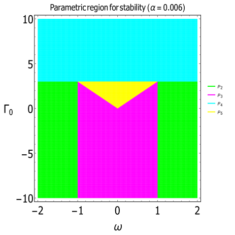
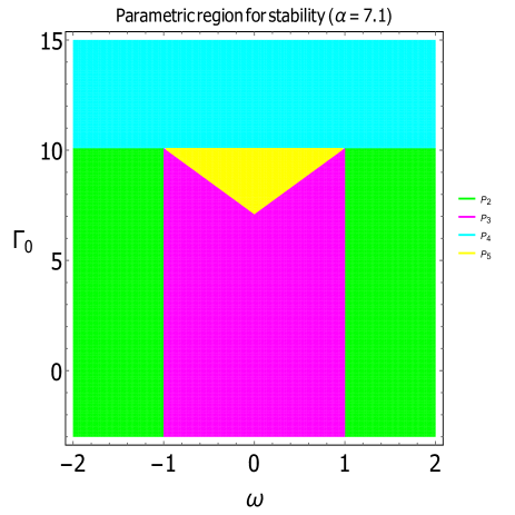
  Figure 1: The figure shows regions of stability of critical points $P_{2},P_{3},P_{4},P_{5}$ in the $(\omega,\Gamma_{0})$ parameter space for $\alpha=0.006$ in panel (a) and $\alpha=7.1$ in panel (b). Here, green shaded region corresponds to the region of stability of point $P_{2}$, magenta shaded region corresponds to the region of stability of point $P_{3}$, cyan shaded region corresponds to the region of stability of point $P_{4}$ and yellow shaded region corresponds to the region of stability of point $P_{5}$.

  

  

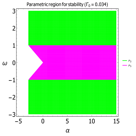
  Figure 2: The figure shows regions of stability of critical points $P_{2},P_{3},P_{4},P_{5}$ in the $(\alpha,\omega)$ parameter space for $\Gamma_{0}=0.034$ in panel (a) and $\Gamma_{0}=10.3095$ in panel (b). Here, green shaded region corresponds to the region of stability of point $P_{2}$, magenta shaded region corresponds to the region of stability of point $P_{3}$, cyan shaded region corresponds to the region of stability of point $P_{4}$ and yellow shaded region corresponds to the region of stability of point $P_{5}$.

  

  

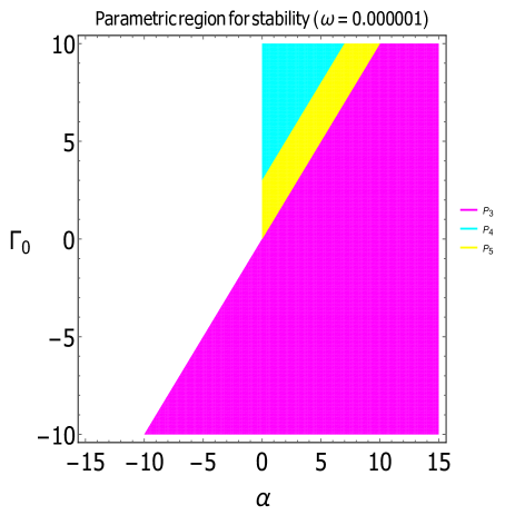
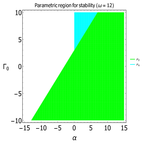
  Figure 3: The figure shows regions of stability of critical points $P_{2},P_{3},P_{4},P_{5}$ in the $(\alpha,\Gamma_{0})$ parameter space for $\omega=0.000001$ in panel (a) and $\omega=12$ in panel (b). Here, green shaded region corresponds to the region of stability of point $P_{2}$, magenta shaded region corresponds to the region of stability of point $P_{3}$, cyan shaded region corresponds to the region of stability of point $P_{4}$ and yellow shaded region corresponds to the region of stability of point $P_{5}$.

  

  

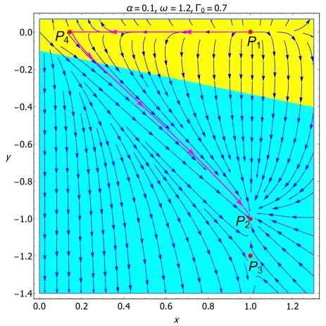
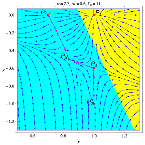
  Figure 4: The phase plot of the autonomous system (33) on the x-y plane for different parameter values: In sub-figure 4 for $\alpha=0.1,~{}~{}\omega=1.2,~{}~{}\Gamma_{0}=0.7$ the point $P_{2}$ exhibits the late time de Sitter solution, point $P_{4}$ is matter dominated saddle-like solution and the point $P_{1}$ is DE dominated decelerated past attractor. Also, the point $P_{3}$ is DE dominated saddle-like solution. The sub-figure 4 shows for $\alpha=7.7,~{}~{}\omega=0.6,~{}~{}\Gamma_{0}=11$ that the point $P_{2}$ is the early de Sitter solution, points $P_{3}$, $P_{5}$ are DE dominated saddle-like solutions. The point $P_{4}$ is DE dominated accelerated scaling attractor. The point $P_{1}$ is DE dominated decelerated past attractor. The point $P_{3}$ is DE dominated accelerated saddle-like solution. Here, the cyan-shaded region represents the accelerated region (i.e. $q<0$) and the yellow-shaded region corresponds to the decelerated region (i.e. $q>0$).

• Critical point $P_{4}$ corresponds to DE-DM scaling solution ($\Omega_{d}\sim\Omega_{m}$) in the phase plane. It exists for the following conditions:

  $(i)~{}[\alpha<0~{}~{}\mbox{and}~{}~{}\Gamma_{0}\leq\alpha],~{}~{}\mbox{or}~{}~{}\\ (ii)~{}[\alpha=0~{}~{}\mbox{and}~{}~{}(\Gamma_{0}<0~{}~{}\mbox{or}~{}~{}\Gamma_{0}>0)],~{}~{}\mbox{or}~{}~{}\\ (iii)~{}[\alpha>0~{}~{}\mbox{and}~{}~{}\Gamma_{0}\geq\alpha]$. The ratio of DE and DM for this case is $r=\frac{\Omega_{d}}{\Omega_{m}}=\frac{\alpha}{\Gamma_{0}-\alpha}.$ That is, for $\Gamma_{0}\longrightarrow\alpha$ the energy density of the DE in the Friedmann equation (13) dominates over the DM ($\Omega_{m}\longrightarrow 0,~{}\Omega_{d}\longrightarrow 1$ see table 1). However, the DE equation of state associated to this critical point always behaves as dust (since $\gamma_{d}=0$). Restrictions on the parameters in the expression of effective equation of state $\omega_{eff}$($=-\frac{\Gamma_{0}}{3}(1-\frac{\alpha}{\Gamma_{0}})$) (in table 1) will show different dynamic phases of evolution. In what follows, the point evolves in quintessence era (parameters satisfying $-1<\omega_{eff}<-\frac{1}{3}$) when $\alpha\geq 0~{}~{}\mbox{and}~{}~{}\alpha+1<\Gamma_{0}<\alpha+3$. On the other hand, the point evolves in cosmological constant era (i.e., $\omega_{eff}=-1$) for $\alpha\geq 0~{}~{}\mbox{and}~{}~{}\Gamma_{0}=\alpha+3$ and the point evolves in phantom regime (i.e., $\omega_{eff}<-1$) for $\alpha\geq 0~{}~{}\mbox{and}~{}~{}\Gamma_{0}>\alpha+3$. It is to be mentioned that the acceleration will be occurred for $\alpha\geq 0~{}~{}\mbox{and}~{}~{}\Gamma_{0}>\alpha+1$. The critical point $P_{4}$ is hyperbolic (since all the eigenvalues have non-zero real parts) and corresponds to an unstable source for ($\alpha\leq 0~{}~{}\mbox{and}~{}~{}\Gamma_{0}<\alpha$), saddle for ($\alpha\geq 0~{}~{}\mbox{and}~{}~{}\alpha<\Gamma_{0}<\alpha+3$), and stable attractor for ($\alpha\geq 0~{}~{}\mbox{and}~{}~{}\Gamma_{0}>\alpha+3$). The region of stability for this point is shown in different parameter spaces $(\alpha,~{}\Gamma_{0},~{}\omega)$ that are exhibited in the figs. (1), 2 and (3). In summary, the critical point represents the late-time scaling attractor solution corresponding to accelerated universe attracted only in phantom era (satisfying $\lambda_{1}<0,~{}~{}\lambda_{2}<0,~{}~{}\mbox{and}~{}~{}\omega_{eff}<-1$) when $\alpha\geq 0~{}~{}\mbox{and}~{}~{}\Gamma_{0}>\alpha+3$, and in this case, DE behaves as dust. This is confirmed numerically by plotting figures. Fig. 10, fig. 10 and fig. 10 exhibit that the late-time accelerated scaling attractor represented by point $P_{4}$ is attracted in phantom regime for the parameter values $\alpha=7.1,~{}\omega=0.005,~{}\Gamma_{0}=10.3095$. Also, Fig. 4 shows that the point $P_{4}$ is late time accelerated scaling attractor for $\alpha=7.7,~{}\omega=0.6,~{}\Gamma_{0}=11.$ Moreover, in a specific parameter region, the point can behave as DM dominated solution. For example: in the limit $\Gamma_{0}\longrightarrow\alpha$ the DE (dust) dominates ($\Omega_{d}\longrightarrow 1$) the cosmological dynamics over DM and the solution represents decelerated universe in dust era ($\omega_{eff}\longrightarrow 0,~{}q\longrightarrow\frac{1}{2}$) when the DE behaves as dust ($\gamma_{d}=0$). In this case, the point will be unstable since one of the eigenvalues will always be positive. This solution represents transient state of evolution. On the other hand, when $\alpha\longrightarrow 0$, (i.e., for uncoupled case) DM dominates over the DE ($\Omega_{m}\longrightarrow 1$) and the dynamics of scaling solution completely depends on the parameter $\Gamma_{0}$. In this case, the effective equation of state parameter reduces to the limit $\omega_{eff}\longrightarrow-\frac{\Gamma_{0}}{3}$, and stability of the point is determined by the eigenvalues: $\lambda_{1}\longrightarrow-\Gamma_{0}$, $\lambda_{2}\longrightarrow-2(\Gamma_{0}-3)$. This is obvious from the above analysis that the point can be physically relevant solution for $0<\Gamma_{0}<1$, i.e., when it is completely dominated by DM representing the intermediate phase of the universe.

• Another DE-DM scaling solution ($\Omega_{d}\sim\Omega_{m}$) represented by the critical point $P_{5}$ exists for the following conditions:

  $(i)~{}(\alpha<0~{}~{}\mbox{and}~{}~{}\Gamma_{0}\leq\alpha+3|\omega|),~{}~{}\mbox{or}~{}~{}\\ (ii)~{}[\alpha=0~{}~{}\mbox{and}~{}~{}(\Gamma_{0}<3|\omega|~{}~{}\mbox{or}~{}~{}\Gamma_{0}>3|\omega|)],~{}~{}\mbox{or}~{}~{}\\ (iii)~{}(\alpha>0~{}~{}\mbox{and}~{}~{}\Gamma_{0}\geq\alpha+3|\omega|)$. The ratio of DE and DM is $r=\frac{\Omega_{d}}{\Omega_{m}}=\frac{\alpha}{\Gamma_{0}-\alpha-3|\omega|}.$ So, depending upon parameter restrictions, either DE can dominate the cosmological dynamics over the DM, or the DM dominates over DE in their evolution. Specifically, the point can be a DE dominated solution ($\Omega_{m}\longrightarrow 0,~{}\Omega_{d}\longrightarrow 1$ see table 1) for $\alpha\neq 0~{}~{}\mbox{and}~{}~{}(\Gamma_{0}-\alpha)\longrightarrow 3|\omega|$ while it will be a DM dominated solution for $\alpha\longrightarrow 0$. The DE associated to this critical point behaves as an exotic type fluid with equation of state $\gamma_{d}=-|\omega|$. Therefore, depending on $\omega$, DE can describe the quintessence, cosmological constant, or phantom field, or any other perfect fluid. Acceleration of the universe near the critical point is possible for the following conditions: ($q<0,~{}\omega_{eff}<-\frac{1}{3}$):

  1. $\left\{\alpha<0~{}~{}\mbox{and}~{}~{}\Gamma_{0}>\alpha+1~{}~{}\mbox{and}~{}~{}\left(\omega\leq-\frac{\Gamma_{0}-\alpha}{3}~{}~{}\mbox{or}~{}~{}\omega\geq\frac{\Gamma_{0}-\alpha}{3}\right)\right\}$

  2. $\left\{\alpha=0~{}~{}\mbox{and}~{}~{}\Gamma_{0}>1~{}~{}\mbox{and}~{}~{}\left(\omega<-\frac{\Gamma_{0}}{3}~{}~{}\mbox{or}~{}~{}-\frac{\Gamma_{0}}{3}<\omega<\frac{\Gamma_{0}}{3}~{}~{}\mbox{or}~{}~{}\omega>\frac{\Gamma_{0}}{3}\right)\right\}$

  3. $\left(\alpha>0~{}~{}\mbox{and}~{}~{}\Gamma_{0}>\alpha+1~{}~{}\mbox{and}~{}~{}-\frac{\Gamma_{0}-\alpha}{3}\leq\omega\leq\frac{\Gamma_{0}-\alpha}{3}\right)$.

  The effective equation of state ($\omega_{eff}$) associated to this critical point determines the universe’s evolution in different phases like: quintessence phase, cosmological constant era, or phantom regime or sometimes dust. In particular, evolution of the universe will be in quintessence era ($-1<\omega_{eff}<-\frac{1}{3}$) for:

  1. $\alpha<0:~{}~{}\\ (i)~{}(\omega\leq-1~{}~{}\mbox{and}~{}~{}\alpha+1<\Gamma_{0}<\alpha+3),~{}~{}\mbox{or}~{}~{}\\ (ii)~{}\left(-1<\omega<-\frac{1}{3}~{}~{}\mbox{and}~{}~{}\alpha+1<\Gamma_{0}\leq\alpha-3\omega\right),~{}~{}\mbox{or}~{}~{}\\ (iii)~{}\left(\frac{1}{3}<\omega<1~{}~{}\mbox{and}~{}~{}\alpha+1<\Gamma_{0}\leq\alpha+3\omega\right),~{}~{}\mbox{or}~{}~{}\\ (iv)~{}(\omega\geq 1~{}~{}\mbox{and}~{}~{}\alpha+1<\Gamma_{0}<\alpha+3)$

  2. $\alpha=0:~{}~{}\\ (i)~{}(\omega\leq-1~{}~{}\mbox{and}~{}~{}1<\Gamma_{0}<3),~{}~{}\mbox{or}~{}~{}\\ (ii)~{}[-1<\omega<-\frac{1}{3}~{}~{}\mbox{and}~{}~{}(1<\Gamma_{0}<-3\omega~{}~{}\mbox{or}~{}~{}-3\omega<\Gamma_{0}<3)],~{}~{}\mbox{or}~{}~{}\\ (iii)~{}\left(-\frac{1}{3}\leq\omega\leq\frac{1}{3}~{}~{}\mbox{and}~{}~{}1<\Gamma_{0}<3\right),~{}~{}\mbox{or}~{}~{}\\ (iv)~{}[\frac{1}{3}<\omega<1~{}~{}\mbox{and}~{}~{}(1<\Gamma_{0}<3\omega~{}~{}\mbox{or}~{}~{}3\omega<\Gamma_{0}<3)],~{}~{}\mbox{or}~{}~{}\\ (v)(\omega\geq 1~{}~{}\mbox{and}~{}~{}1<\Gamma_{0}<3)$

  3. $\alpha>0:~{}~{}\\ (i)~{}(-1<\omega<-\frac{1}{3}~{}~{}\mbox{and}~{}~{}\alpha-3\omega\leq\Gamma_{0}<\alpha+3),~{}~{}\mbox{or}~{}~{}\\ (ii)~{}\left(-\frac{1}{3}\leq\omega\leq\frac{1}{3}~{}~{}\mbox{and}~{}~{}\alpha+1<\Gamma_{0}<\alpha+3\right),~{}~{}\mbox{or}~{}~{}\\ (iii)\left(\frac{1}{3}<\omega<1~{}~{}\mbox{and}~{}~{}\alpha+3\omega\leq\Gamma_{0}<\alpha+3\right)$,

  in cosmological constant era for:

  1. $\Gamma_{0}=\alpha+3:~{}~{}\\ (i)~{}[\alpha<0~{}~{}\mbox{and}~{}~{}(\omega\leq-1~{}~{}\mbox{or}~{}~{}\omega\geq 1)],~{}~{}\mbox{or}~{}~{}\\ (ii)~{}[\alpha=0~{}~{}\mbox{and}~{}~{}(\omega<-1~{}~{}\mbox{or}~{}~{}-1<\omega<1~{}~{}\mbox{or}~{}~{}\omega>1)],~{}~{}\mbox{or}~{}~{}\\ (iii)~{}(\alpha>0~{}~{}\mbox{and}~{}~{}-1\leq\omega\leq 1)$,

  and in phantom era for:

  1. $[\alpha<0~{}~{}\mbox{and}~{}~{}\left\{(\omega<-1~{}~{}\mbox{and}~{}~{}\alpha+3<\Gamma_{0}\leq\alpha-3\omega)~{}~{}\mbox{or}~{}~{}(\omega>1~{}~{}\mbox{and}~{}~{}\alpha+3<\Gamma_{0}\leq\alpha+3\omega)\right\}]$

  2. $\alpha=0:~{}~{}\\ (i)~{}[\omega<-1~{}~{}\mbox{and}~{}~{}(3<\Gamma_{0}<-3\omega~{}~{}\mbox{or}~{}~{}\Gamma_{0}>-3\omega)],~{}~{}\mbox{or}~{}~{}\\ (ii)~{}(-1\leq\omega\leq 1~{}~{}\mbox{and}~{}~{}\Gamma_{0}>3),~{}~{}\mbox{or}~{}~{}\\ (iii)~{}[\omega>1~{}~{}\mbox{and}~{}~{}(3<\Gamma_{0}<3\omega~{}~{}\mbox{or}~{}~{}\Gamma_{0}>3\omega)]$

  3. $\alpha>0:~{}~{}\\ (i)~{}(\omega<-1~{}~{}\mbox{and}~{}~{}\Gamma_{0}\geq\alpha-3\omega),~{}~{}\mbox{or}~{}~{}\\ (i)~{}(-1\leq\omega\leq 1~{}~{}\mbox{and}~{}~{}\Gamma_{0}>\alpha+3),~{}~{}\mbox{or}~{}~{}\\ (ii)~{}(\omega>1~{}~{}\mbox{and}~{}~{}\Gamma_{0}\geq\alpha+3\omega)$.

  The critical point $P_{5}$ is a hyperbolic in nature since all the eigenvalues have non-zero real parts (presented in table 2). According to linear stability theory, the point describes an unstable source ($\lambda_{1}>0,~{}\lambda_{2}>0$) for :
  $[\alpha\leq 0~{}~{}\mbox{and}~{}~{}\left\{(\omega<-1~{}~{}\mbox{and}~{}~{}\alpha+3<\Gamma_{0}<\alpha-3\omega)~{}~{}\mbox{or}~{}~{}(\omega>1~{}~{}\mbox{and}~{}~{}\alpha+3<\Gamma_{0}<\alpha+3\omega)\right\}].$ On the other hand, the point represents the stable attractor ($\lambda_{1}<0,~{}\lambda_{2}<0$) for:
  $[\alpha\geq 0~{}~{}\mbox{and}~{}~{}\left\{(-1<\omega\leq 0~{}~{}\mbox{and}~{}~{}\alpha-3\omega<\Gamma_{0}<\alpha+3)~{}~{}\mbox{or}~{}~{}(0<\omega<1~{}~{}\mbox{and}~{}~{}\alpha+3\omega<\Gamma_{0}<\alpha+3)\right\}]$. The regions of stability of the critical point in parameter spaces ($\alpha,~{}\Gamma_{0},~{}\omega$) are shown in figs. (1), 2 and 3. The point describes the saddle-like solution ($\lambda_{1}\lambda_{2}<0$) for the following conditions :

  1. $\alpha\geq 0:~{}~{}\\ (i)~{}(\omega\leq-1~{}~{}\mbox{and}~{}~{}\Gamma_{0}>\alpha-3\omega),~{}~{}\mbox{or}~{}~{}\\ (ii)~{}(-1<\omega\leq 1~{}~{}\mbox{and}~{}~{}\Gamma_{0}>\alpha+3),~{}~{}\mbox{or}~{}~{}\\ (iii)~{}(\omega>1~{}~{}\mbox{and}~{}~{}\Gamma_{0}>\alpha+3\omega)$.

  2. $\alpha\leq 0:~{}~{}\\ (i)~{}(\omega\leq-1~{}~{}\mbox{and}~{}~{}\Gamma_{0}<\alpha+3),~{}~{}\mbox{or}~{}~{}\\ (ii)~{}(-1<\omega\leq 0~{}~{}\mbox{and}~{}~{}\Gamma_{0}<\alpha-3\omega),~{}~{}\mbox{or}~{}~{}\\ (iii)~{}(0<\omega\leq 1~{}~{}\mbox{and}~{}~{}\Gamma_{0}<\alpha+3\omega),~{}~{}\mbox{or}~{}~{}\\ (iv)~{}(\omega>1~{}~{}\mbox{and}~{}~{}\Gamma_{0}<\alpha+3)$

  Saddle solution arises due to instability in one eigendirection associated with positive eigenvalue and stability in another eigendirection associated with negative eigenvalue. In summary, one can conclude that the critical point $P_{5}$ corresponding to the late-time accelerated scaling attractor is achieved only in quintessence era ($\lambda_{1}<0,~{}~{}\lambda_{2}<0,~{}~{}\mbox{and}~{}~{}-1<\omega_{eff}<-\frac{1}{3}$) for : $\alpha\geq 0~{}~{}\mbox{and}~{}~{}$
  (i)  $(-1<\omega\leq-\frac{1}{3}~{}~{}\mbox{and}~{}~{}\alpha-3\omega<\Gamma_{0}<\alpha+3),~{}~{}\mbox{or}~{}~{}\\ (ii)~{}\left(-\frac{1}{3}<\omega\leq\frac{1}{3}~{}~{}\mbox{and}~{}~{}\alpha+1<\Gamma_{0}<\alpha+3\right),~{}~{}\mbox{or}~{}~{}\\ (iii)~{}\left(\frac{1}{3}<\omega<1~{}~{}\mbox{and}~{}~{}\alpha+3\omega<\Gamma_{0}<\alpha+3\right).$ It is interesting to note that the point in this case, can alleviate the coincidence problem due to having $0<\Omega_{d}<1$ where DE behaves as quintessence. Fig. (5) for $\alpha=0.2,~{}\omega=0.57,~{}\Gamma_{0}=2$ shows that the scaling solution $P_{5}$ exhibits the accelerated attractor at late-time attracted in quintessence era. Further, it should be mentioned that for particular choice of parameters, the critical point corresponds to either DE or DM dominated solution. In particular, for ($\Gamma_{0}-\alpha)\longrightarrow 3|\omega|$, DE dominates the cosmological dynamics $\Omega_{d}\longrightarrow 1$, as a result of which the effective equation of state becomes $\omega_{eff}\longrightarrow-|\omega|$ which corresponding to accelerated evolution in quintessence era at late times. While, for $\alpha\longrightarrow 0$, DM energy density dominates the cosmological dynamics ($\Omega_{m}\longrightarrow 1$) in Friedmann equation. In this case, $\omega_{eff}\longrightarrow-\frac{\Gamma_{0}}{3}$ which implies that acceleration is possible only when $\Gamma_{0}>1$ and the corresponding eigenvalues are $\lambda_{1}\longrightarrow-2(-\Gamma_{0}+3)$ and $\lambda_{2}\longrightarrow-\Gamma_{0}+3|\omega|$ which results the critical point’s stability when $3|\omega|<\Gamma_{0}<3$. Therefore, an accelerating DM dominated late-time solution is achieved through this critical point and this result is nonphysical due to present observational data. Therefore, only physically relevant solution in this case will be the matter dominated decelerating transient phase of the universe which is achieved in the parameter region : $\Gamma_{0}<\mbox{min}\{1,~{}~{}3|\omega|\}.$

  

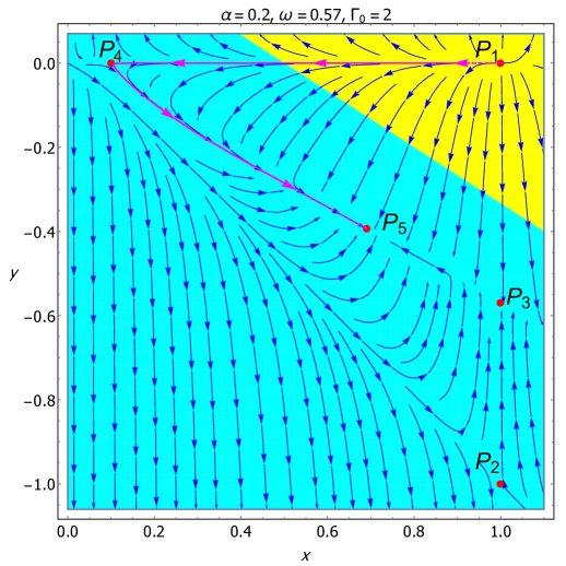
  Figure 5: The figure shows the phase plane of the autonomous system (33) on the x-y plane for the parameter values: $\alpha=0.2,~{}~{}\omega=0.57,~{}~{}\Gamma_{0}=2$. The point $P_{5}$ is accelerated scaling attractor. The point $P_{1}$ is DE dominated decelerated past attractor where DE behaves as dust. Point $P_{4}$ is matter dominated accelerated saddle-like solution. The point $P_{3}$ is DE dominated accelerated saddle-like solution. The point $P_{2}$ is de Sitter solution describing transient phase. Here, the cyan shaded region represents the accelerated region (i.e. $q<0$) and the yellow shaded region corresponds to the decelerated region (i.e. $q>0$).

• The set of critical points $P_{6}$ exists for the following conditions: ($0\leq x_{c}\leq 1~{}~{}\mbox{and}~{}~{}\Gamma_{0}=\alpha+3$). The set corresponds to a solution with combination of both DE and DM. The ratio of DE and DM is $r=\frac{\Omega_{d}}{\Omega_{m}}=\frac{x_{c}}{1-x_{c}}$. A point on this set will become completely DE dominated for $x_{c}=1$ ($\Omega_{m}=0,~{}\Omega_{d}=1$ see table 1). The DE behaves as a perfect fluid with equation of state $\gamma_{d}=\frac{\alpha-x_{c}(\alpha+3)}{3x_{c}}$. Depending on $x_{c}$ and the parameter $\alpha$, the DE corresponds to quintessence, cosmological constant or phantom fluid, or any other exotic type fluid. The expansion of the universe will always be accelerating in phase plane (since $\omega_{eff}=-1$, $q=-1$).
  The set of critical points $P_{6}$ is a non-isolated set having exactly one vanishing eigenvalue. This set is called normally hyperbolic set [114] and to find the stability of this set, one has to keep attention on the sign of remaining non-zero eigenvalue. However, the set will be stable for the following conditions :

  1. $\Gamma_{0}=\alpha+3~{}~{}\mbox{and}~{}~{}(0<x_{c}<1):~{}~{}\\ (i)~{}~{}\left\{\omega<0~{}~{}\mbox{and}~{}~{}-\frac{3x_{c}}{4(x_{c}-1)}\left(\sqrt{(\omega-8)\omega}+(\omega+4)\right)<\alpha<\frac{3x_{c}}{4(x_{c}-1)}\left(\sqrt{(\omega-8)\omega}-(\omega+4)\right)\right\},~{}~{}\mbox{or}~{}~{}\\ (ii)~{}~{}\left\{\omega>0~{}~{}\mbox{and}~{}~{}\frac{3x_{c}}{4(x_{c}-1)}\left(\omega-4-\sqrt{\omega(\omega+8)}\right)<\alpha<\frac{3x_{c}}{4(x_{c}-1)}\left(\sqrt{\omega(\omega+8)}+\omega-4\right)\right\}$

  2. $\Gamma_{0}=\alpha+3~{}~{}\mbox{and}~{}~{}\left\{x_{c}=1~{}~{}\mbox{and}~{}~{}(\omega<-1~{}~{}\mbox{or}~{}~{}\omega>1)\right\}$.

  Also, the set $P_{6}$ will be unstable for the following conditions :

  1. $\Gamma_{0}=\alpha+3~{}~{}\mbox{and}~{}~{}(0<x_{c}<1):~{}~{}\\ (i)~{}~{}\omega<0~{}~{}\mbox{and}~{}~{}\left\{\alpha<-\frac{3x_{c}}{4(x_{c}-1)}\left(\sqrt{(\omega-8)\omega}+(\omega+4)\right)~{}~{}\mbox{or}~{}~{}\alpha>\frac{3x_{c}}{4(x_{c}-1)}\left(\sqrt{(\omega-8)\omega}-(\omega+4)\right)\right\},~{}~{}\mbox{or}~{}~{}\\ (ii)~{}~{}\omega>0~{}~{}\mbox{and}~{}~{}\left\{\alpha<\frac{3x_{c}}{4(x_{c}-1)}\left(\omega-4-\sqrt{\omega(\omega+8)}\right)~{}~{}\mbox{or}~{}~{}\alpha>\frac{3x_{c}}{4(x_{c}-1)}\left(\sqrt{\omega(\omega+8)}+\omega-4\right)\right\}$

  2. $\Gamma_{0}=\alpha+3~{}~{}\mbox{and}~{}~{}\left\{x_{c}=1~{}~{}\mbox{and}~{}~{}(-1<\omega<0~{}~{}\mbox{or}~{}~{}0<\omega<1)\right\}$.

  The fig. (7) for $\alpha=7.1,~{}\omega=1.1,~{}\Gamma_{0}=10.1$ shows that the set of critical points on the line bounded in $0.609552<x_{c}\leq 1$ is stable in the phase plane. It is interesting to note that the set represents completely DE dominated solution for $x_{c}=1$. For this case, the cosmological parameters take the values: $\Omega_{m}=0,~{}~{}\Omega_{d}=1,~{}~{}\omega_{eff}=q=-1$ and the eigenvalues: $\lambda_{1}=0,~{}~{}\lambda_{2}=-6+\frac{6}{|\omega|}$. The DE behaves as cosmological constant ($\gamma_{d}=-1$) for this case. For this particular value of $x_{c}$, actually the point $P_{6}$ becomes a point with coordinate ($1,~{}\frac{\alpha-\Gamma_{0}}{3}$) and this point corresponds to de Sitter expansion of evolution. However, the point having one vanishing eigenvalue is now becoming a non-hyperbolic type critical point and due to importance of this type of solution in cosmological context, we shall show the stability of the point numerically. The point will show a stable solution for $|\omega|>1$ because there exists a non-empty stable submanifold in the negative eigendirection. On the other hand, the point on the set may represent the early accelerated de Sitter solution for $|\omega|<1$, because there is an non-empty unstable sub-manifold in the positive eigendirection. In fig.(8), for $\alpha=7.1,~{}\omega=1.1,~{}\Gamma_{0}=10.1$ the point with coordinate $(1,~{}-1)$ on the set corresponds to late time accelerated de Sitter solution because the perturbations are coming into $x=1$ and $y=-1$ in this case. On the other hand, the fig.(9) with $\alpha=7.1,~{}\omega=0.6,~{}\Gamma_{0}=10.1$ exhibits that the point on the set describes the accelerated de Sitter solution which is past attractor because for this case, the perturbations are coming out from $x=1$ and $y=-1$. For $x_{c}\longrightarrow 0$, the set corresponds to the DM dominated solution. But, due to ever accelerating nature, the point cannot be represent the intermediate phase of the universe. So, in this case, it is unrealistic from cosmological point of view. Finally, for $x_{c}=\frac{\alpha}{\Gamma_{0}}$, the set will be the critical point $P_{4}$ which has already been discussed.

  

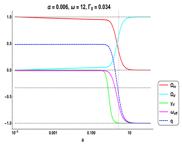
  Figure 6: The figure shows the evolution of cosmological parameters for the values of free parameters: $\alpha=0.006,~{}~{}\omega=12,~{}~{}\Gamma_{0}=0.034$. Here, the trajectories are attracted by cosmological constant at late-times connecting through a matter-dominated decelerated phase.

  

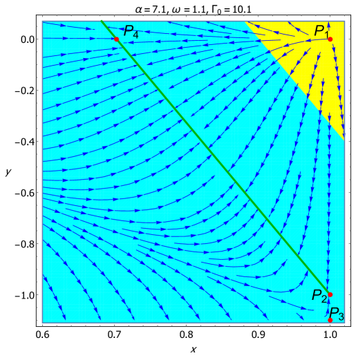
  Figure 7: The figure shows the vector field of the autonomous system (33) on the x-y plane for the parameter values: $\alpha=7.1,~{}~{}\omega=1.1,~{}~{}\Gamma_{0}=10.1$. The set $P_{6}$ represented by the green colored line shows the stable attractor. The point $P_{1}$ is DE dominated decelerated source. But the point $P_{3}$ gives DE dominated accelerated saddle-like solution. Here, the cyan shaded region represents the accelerated region (i.e. $q<0$) and the yellow shaded region corresponds to the decelerated region (i.e. $q>0$).

  

  

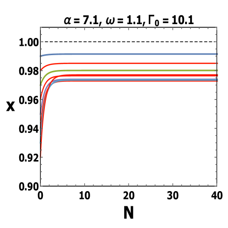
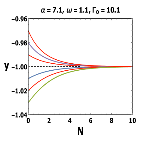
  Figure 8: The figure shows the time evolution of trajectories of x and y for the critical point $P_{6}$ for parameter values $\alpha=7.1$, $\omega=1.1$ and $\Gamma_{0}=10.1$.

  

  

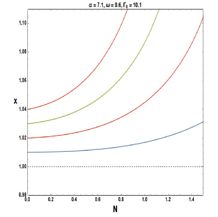
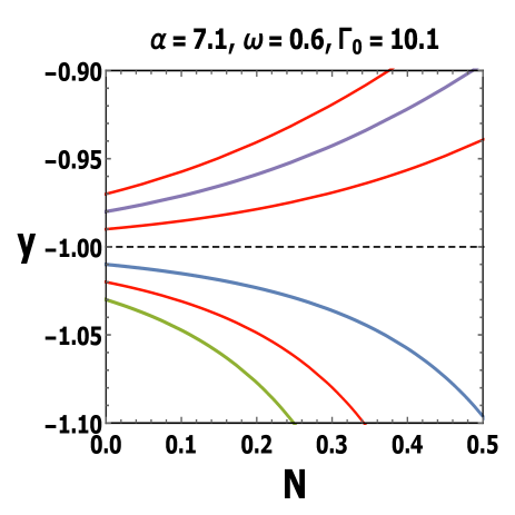
  Figure 9: The figure shows the projection of time evolution of the phase space trajectories of perturbation of the autonomous system (33) along the x and y axes for the critical point $P_{6}$ for parameter values $\alpha=7.1$, $\omega=0.6$ and $\Gamma_{0}=10.1$.

IV.2 Classical stability of the model :

The local stability of the critical points extracted from the autonomous system is characterized by the eigenvalues of perturbation matrix (presented in table) and the stability criteria are discussed in detail in the previous section. Now, we shall discuss the classical stability of the model. In cosmological perturbation, the sound speed ($C_{s}^{2}$), appearing as coefficient of the term $\frac{k^{2}}{a(t)^{2}}$ (where $k$ is the co-moving momentum and $a(t)$ is the usual scale factor), plays a vital role to determine the classical stability of the model. The sound speed can be defined as [117, 118, 115, 116, 119, 120]

$$C_{s}^{2}=\frac{\partial p_{d}}{\partial\rho_{d}}$$ (34)

The classical fluctuations of the model is considered to be stable only when the sound speed $C_{s}^{2}$ is positive i.e., $C_{s}^{2}\geq 0$. On the other hand, it violates the causality when $C_{s}^{2}>1$, i.e., when the speed of sound diverges. Moreover, ghost instabilities can be realized for $C_{s}^{2}<0$. In the present work, we shall investigate the classical stability of the model, avoiding the ghost instabilities. For that we shall find $\frac{\partial p_{d}}{\partial\rho_{d}}$ (described in Eqn. (34)) for the present cosmological model explicitly in terms of dynamical variables and free parameters. With the help of Eqn.(16), we obtain the following

$$C_{s}^{2}=\frac{\partial p_{d}}{\partial\rho_{d}}=\frac{\frac{\rho_{d}^{2}}{|A|}-\frac{1}{|\omega|}}{\left(\frac{\rho_{d}^{2}}{|A|}+\frac{1}{|\omega|}\right)^{2}}$$ (35)

After that for simplifying, we use Eqn.(22) in the above equation which will give the following:

$$C_{s}^{2}=\frac{\frac{9x^{2}H^{4}}{|A|}-\frac{1}{|\omega|}}{\left(\frac{9x^{2}H^{4}}{|A|}+\frac{1}{|\omega|}\right)^{2}}$$ (36)

and finally, from (24) and (22) we obtained the expression of sound speed in terms of dynamical variables as follows:

$$C_{s}^{2}=-\left(\frac{y}{x}+\frac{2y^{2}}{|\omega|x^{2}}\right).$$ (37)

Therefore, one can easily obtain the condition for classical stability from the above as:

$$-\left(\frac{y}{x}+\frac{2y^{2}}{|\omega|x^{2}}\right)\geq 0.$$ (38)

The inequality (38) shows the classical stability criteria for the present model. We shall now discuss the classical stability of the model at each critical point where $x$ and $y$ are the co-ordinates of the corresponding critical point. We observe that

• The critical point $P_{1}$ corresponds to classical stability for all free parameters $\alpha$, $\omega$ and $\Gamma_{0}$.

• The critical point $P_{2}$ is stable classically for either $\omega\leq-2~{}~{}\mbox{or}~{}~{}\omega\geq 2$.

• The critical point $P_{3}$ corresponds to classically stable for $\omega=0$.

• The critical point $P_{4}$ shows classical stability for all parameters $\alpha$, $\omega$ and $\Gamma_{0}$.

• Condition for classical stability of the critical point $P_{5}$ is $\omega=0$.

• Finally, the set of points $P_{6}$ is stable classically for the following parameter restrictions:

  1. $\Gamma_{0}=\alpha+3~{}~{}\mbox{and}~{}~{}(0<x_{c}<1):~{}~{}\\ (i)~{}~{}\left\{\omega<0~{}~{}\mbox{and}~{}~{}\frac{3x_{c}(\omega+2)}{(1-x_{c})2}\leq\alpha\leq\frac{3x_{c}}{1-x_{c}}\right\},~{}~{}\mbox{or}~{}~{}\\ (ii)~{}~{}\left\{\omega>0~{}~{}\mbox{and}~{}~{}\frac{3x_{c}(2-\omega)}{(1-x_{c})2}\leq\alpha\leq\frac{3x_{c}}{1-x_{c}}\right\}$

  2. $\Gamma_{0}=\alpha+3~{}~{}\mbox{and}~{}~{}\left\{x_{c}=1~{}~{}\mbox{and}~{}~{}(\omega\leq-2~{}~{}\mbox{or}~{}~{}\omega\geq 2)\right\}$.

From the above analysis of classical stability of the model and the local stability of the critical points, the points can be classified into different categories such as: there may be unstable critical points at which the model is stable. On the other hand, there may exist some points which are locally stable critical points at which the model may unstable or stable.

• The critical point $P_{1}$ is stable classically for all $\alpha$, $\omega$ and $\Gamma_{0}$, but not stable locally for any value of $\alpha$, $\omega$ and $\Gamma_{0}$.

• The critical point $P_{2}$ is stable locally as well as classically for :
  $\left\{(\omega\leq-2~{}~{}\mbox{and}~{}~{}\Gamma_{0}<\alpha+3)~{}~{}\mbox{or}~{}~{}(\omega\geq 2~{}~{}\mbox{and}~{}~{}\Gamma_{0}<\alpha+3)\right\}$.

• The critical point $P_{3}$ is stable locally as well as classically for $(\omega=0~{}~{}\mbox{and}~{}~{}\Gamma_{0}<\alpha)$.

• The critical point $P_{4}$ is stable locally as well as classically for $(\alpha\geq 0~{}~{}\mbox{and}~{}~{}\Gamma_{0}>\alpha+3)$.

• The point $P_{5}$ is stable locally as well as classically when the following conditions are satisfied:
  (i) $(\alpha=0~{}~{}\mbox{and}~{}~{}\omega=0~{}~{}\mbox{and}~{}~{}0<\Gamma_{0}<3)$,  or
  (ii) $(\alpha>0~{}~{}\mbox{and}~{}~{}\omega=0~{}~{}\mbox{and}~{}~{}\alpha<\Gamma_{0}<\alpha+3)$.

• Finally, the set of points $P_{6}$ is locally as well as classically stable for the following parameter restrictions:

  1. $\Gamma_{0}=\alpha+3~{}~{}\mbox{and}~{}~{}(0<x_{c}<1):~{}~{}\\ (i)~{}~{}\left\{\omega<0~{}~{}\mbox{and}~{}~{}\frac{3x_{c}(\omega+2)}{(1-x_{c})2}\leq\alpha\leq\frac{3x_{c}}{1-x_{c}}\right\},~{}~{}\mbox{or}~{}~{}\\ (ii)~{}~{}\left\{\omega>0~{}~{}\mbox{and}~{}~{}\frac{3x_{c}(2-\omega)}{(1-x_{c})2}\leq\alpha\leq\frac{3x_{c}}{1-x_{c}}\right\}$

  2. $\Gamma_{0}=\alpha+3~{}~{}\mbox{and}~{}~{}\left\{x_{c}=1~{}~{}\mbox{and}~{}~{}(\omega\leq-2~{}~{}\mbox{or}~{}~{}\omega\geq 2)\right\}$.

V Cosmological interpretation of the critical points

We shall now discuss the cosmology behind the critical points arising from the autonomous system (33) in the previous section. The local stability of the critical points are presented in the section IV.1 where a detailed phase plane analysis is performed. The main findings from the analysis are as follows:
First of all, the autonomous system admits three Umami Chaplygin fluid (DE) dominated solutions, namely the critical points $P_{1}$, $P_{2}$ and $P_{3}$ in the phase plane. The critical point $P_{1}$ corresponds to Umami Chaplygin fluid (DE) dominated decelerated universe in dust era ($q=\frac{1}{2},~{}\omega_{eff}=0$) where the Umami Chaplygin gas behaves as dust ($\gamma_{d}$=0). From the stability analysis, it is observed that the parameter restriction $\Gamma_{0}>\alpha$ describes the early evolution (because the solution is source here) corresponding to dust dominated decelerating phase of the universe. On the other hand, for $\Gamma_{0}<\alpha$, being a saddle-like solution in phase plane, the critical point $P_{1}$ corresponds to a dust dominated decelerating universe representing intermediate phase of evolution. This is the only physically relevant solution represented by $P_{1}$. The de Sitter expansion of the universe is realized by the critical point $P_{2}$ which may represent early as well as late phase of the universe. If we constrain the parameters as $|\omega|<1,~{}(\Gamma_{0}-\alpha)>3$, it is observed that the critical point describes a past attractor in phase plane and the point corresponds to early accelerated de Sitter expansion of the universe ($\Omega_{d}=1,~{}\Omega_{m}=0,~{}\omega_{eff}=-1,~{}q=-1$), whereas the parameter restriction $|\omega|>1,~{}(\Gamma_{0}-\alpha)<3$ indicates that the point is a late-time de Sitter solution describing the accelerated expansion of the universe and this acceleration is governed by the Umami Chaplygin gas ($\gamma_{d}=-1$). These phenomena are also confirmed numerically which are presented in figure (4). In sub-fig. 4, it is shown for $\alpha=7.7,~{}\omega=0.6,~{}\Gamma_{0}=11$ that the universe’s evolution starting from early accelerated de Sitter solution ($P_{2}$) to late-time accelerated scaling attractor (represented by $P_{4}$). Another sub-fig. 4 for the parameter values $\alpha=0.1,~{}\omega=1.2,~{}\Gamma_{0}=0.7$ shows that the late-time de Sitter phase (represented by $P_{2}$) is the ultimate fate of the universe. In this figure, it is also shown that the point $P_{4}$ is the matter-dominated saddle solution representing the intermediate phase of universe connecting through early (source) Umami Chaplygin fluid dominated decelerated phase of the universe (represented by the point $P_{1}$) where the Umami Chaplygin fluid mimics as dust ($\gamma_{d}=0$).
Another Umami Chaplygin fluid dominated universe is represented by the critical point $P_{3}$ which will be able to show different cosmic phases for different choices of model parameters. However, a physically relevant solution is achieved only when it evolves in quintessence era at late-times where the DE behaves as quintessence fluid. This is discussed in detail in the previous section IV.1.

Next, the autonomous system (33) extracts three scaling solutions namely, $P_{4}$, $P_{5}$ and $P_{6}$ in the phase plane and they exhibit some interesting scenarios which are important in cosmological context. The main findings of these points are following: imposing some restrictions on parameters, the scaling solution represented by the point $P_{4}$ can describe the accelerated evolution of the universe attracted in phantom regime at late times. In particular, for parameter values: $\alpha=7.1,~{}\omega=0.005,~{}\Gamma_{0}=10.3095$ the sub-figs. 10, 10, and 10 exhibit that the scaling solution is stable attractor in phase plane satisfying $0<\Omega_{d}<1$ which indicates that this solution can alleviate the coincidence problem. The corresponding physical parameters for this point are: ($\Omega_{m}\approx 0.3,~{}\Omega_{d}\approx 0.7,~{}\omega_{eff}\approx-1.07,~{}q\approx-1.10$). It is interesting to note that the sub-fig. 4 for model parameter values: $\alpha=7.7,~{}\omega=0.6,~{}\Gamma_{0}=11$ also refers to the scaling solution $P_{4}$ which corresponds to accelerated attractor in phantom era at late-times with associated cosmological parameters ($\Omega_{m}=0.3,~{}\Omega_{d}=0.7,~{}\omega_{eff}=-1.1,~{}q=-1.15$). It should be mentioned that for both the cases associated DE represented by the Umami Chaplygin fluid behaves as dust ($\gamma_{d}=0$).

Another interesting scaling solution represented by critical point $P_{5}$ can provide the features of late-time cosmological dynamics of the universe. For some parameter restrictions, the solution corresponds to a late-time accelerated scaling attractor in quintessence era satisfying $0<\Omega_{d}<1$ which can give the possible mechanism to alleviate the coincidence problem. The fig. (5) with the model parameters: $\alpha=0.2,~{}\omega=0.57,~{}\Gamma_{0}=2$ indicates that the solution $P_{5}$ describes late time evolution of the universe in agreement with the observation. In this case the numerical values of the cosmological parameters are: ($\Omega_{m}\approx 0.31,~{}\Omega_{d}\approx 0.69,~{}\omega_{eff}\approx-0.6,~{}q\approx-0.4$). Note that the Umami Chaplygin gas (as the DE candidate) for this case mimics as quintessence ($\gamma_{d}=-0.57$).

Finally, we observe that the scaling solution described by the set of critical points $P_{6}$ can mimic the $\Lambda$CDM model of universe. Fig. (7) with parameter values: $\alpha=7.1,~{}\omega=1.1,~{}\Gamma_{0}=10.1$ shows that the set is stable solution in phase plane with $\omega_{eff}=-1,~{}q=-1$. The evolution of cosmological parameters $\Omega_{m},~{}\Omega_{d},~{}\omega_{eff},~{}q$ in the fig. (6) for the values of model parameters $\alpha=0.006,~{}\omega=12,~{}\Gamma_{0}=0.034$ with proper choice of initial conditions exhibits that the ultimate fate of the universe is described by $\Lambda$CDM.

For a specific choice of $x_{c}=1$, the set represents early time (for $|\omega|<1$) as well as the late phase (for $|\omega|>1$) of de Sitter solution. This is shown by numerical invesigation. For $\alpha=7.1,~{}\omega=1.1,~{}\Gamma_{0}=10.1$, the set $P_{6}$ will become a point with coordinate ($1,~{}-1$) in the phase plane. Here, the fig. (8) describes the accelerating late-time de Sitter universe (as in sub-fig. 8, the trajectories approach in $x=1$ line, as well as in sub-fig.8, the perturbations coming back to $y=-1$ line). On the other hand, early accelerated de Sitter expansion of the universe is realized in fig. (9) for $\alpha=7.1,~{}\omega=0.6,~{}\Gamma_{0}=10.1$ (as in sub-fig. 9 refers to unstable along $x=1$ line and sub-fig. 9 corresponds to instability in $y=-1$ line).

In summary, it is worth mentioning that a region of parameter space ($\alpha,~{}\Gamma_{0},~{}\omega$) can be obtained (see the plot in fig.(11)) in which some critical points exhibit a complete description of evolutionary scheme of universe. For example, we obtained the restrictions: $\omega\in(-1,~{}1),~{}\omega\neq 0$ and $3+\alpha<\Gamma_{0}<2\alpha$, where $\alpha>3$ such that the critical point $P_{2}$ corresponds to Umami Chaplyging fluid dominated early accelerated de Sitter solution representing the early inflation of universe, where the Umami Chaplygin gas behaves as cosmological constant like fluid. Next, the critical point $P_{3}$ describes the decelerated intermediate phase of the universe. In this case, the point $P_{3}$ is actually Umami Chaplygin (DE) dominated solution, however, the universe appears here as if it is DM dominated solution ($\omega_{eff}\longrightarrow 0,$ as $|\omega|\longrightarrow 0$), the matter mimics the perfect fluid nature here and the Umami Chaplygin fluid behaves as perfect fluid. Finally, a late-time scaling attractor is obtained by the point $P_{4}$ which is in a good agreement with the observational data. The sub-figs. 10, and 10 display a sequence of critical points:

$P_{2}$ (source) $\longrightarrow$ $P_{3}$ (saddle) $\longrightarrow$ $P_{4}$ (stable)

which corresponds to a complete description of evolutionary scheme starting from early inflation (represented by $P_{2}$) to late-time acceleration of the universe (described by $P_{4}$) connecting through a sufficient amount of matter dominated decelerated phase (represented by $P_{3}$). The evolution plot of effective equation of state $\omega_{eff}$ and the deceleration parameter $q$ also confirm the above fact. The fig.10 for $\alpha=7.1,~{}\omega=0.000001,~{}\Gamma_{0}=10.3095$ exhibits that the universe’s evolution starting from $\omega_{eff}=q=-1$ (represented by the point $P_{2}$ with $\Omega_{m}=0,~{}\Omega_{d}=1,~{}\gamma_{d}=-1$, i.e, the early de Sitter universe) will go through the phase where $\omega_{eff}\approx 0,~{}q\approx 0.5$ (described by the point $P_{3}$ with $\Omega_{m}=0,~{}\Omega_{d}=1,~{}\gamma_{d}\approx 0$, i.e., the Umami Chaplygin gas mimicking the dust here) and finally will approach to the state where $\omega_{eff}\approx-1.07,~{}q\approx-1.05$ (realized by the point $P_{4}$ with $\Omega_{m}\approx 0.3,~{}\Omega_{d}\approx 0.7$ and $\gamma_{d}=0$.) It is also observed from the plot 10 that there is a possibility of crossing the phantom barrier which is also favored by present observation. It should also be noted that there is a sudden change in the evolution of $\omega_{eff}$ and $q$ from $-1$ to $0$ and from $-1$ to $\frac{1}{2}$ respectively at the same time. This refers to the possibility of bouncing universe and this needs further investigation which we shall discuss in the next section. To realize the early evolution of the universe, we perform a numerical investigation of this model in the next section.

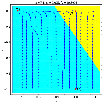
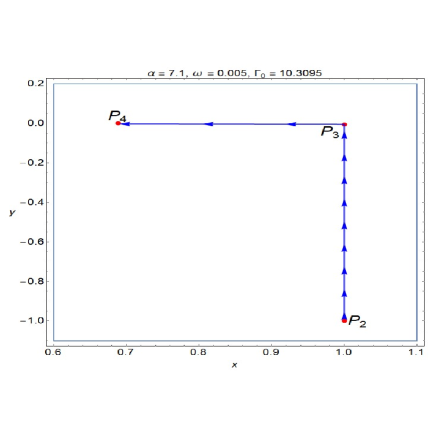
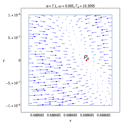
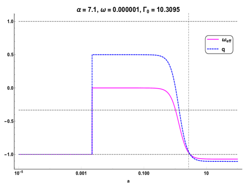
Figure 10: The sub-figures 10, 10 and 10 display the stream plot of the autonomous system (33) on the x-y plane for the parameter values: $\alpha=7.1,~{}~{}\omega=0.005,~{}~{}\Gamma_{0}=10.3095$. The sub-figure 10 shows the point $P_{2}$ is the early de Sitter solution, point $P_{3}$ decelerated saddle-like solution and point $P_{4}$ gives scaling solution which is a stable attractor. Here, the cyan shaded region represents the accelerated region (i.e. $q<0$) and the yellow shaded region corresponds to the decelerated region (i.e. $q>0$). The sub-figure 10 shows a sequence of critical points showing complete evolution of the universe where sub-figure 10 exhibits the late-time attractor $P_{4}$ with $(\Omega_{m}=0.311,\Omega_{d}=0.688,\gamma_{d}=0,\omega_{eff}=-1.069,q=-1.105)$. Sub-figure 10 for $\alpha=7.1,~{}~{}\omega=0.000001,~{}~{}\Gamma_{0}=10.3095$ exhibits the evolution of decelerating parameter $q$ and effective equation of state parameter $\omega_{eff}$ with initial conditions: $x(0)=0.9099999$ and $y(0)=-0.0000009099999$. This shows a unified description of universe from early inflation to late time acceleration connecting through intermediate decelerated phase.

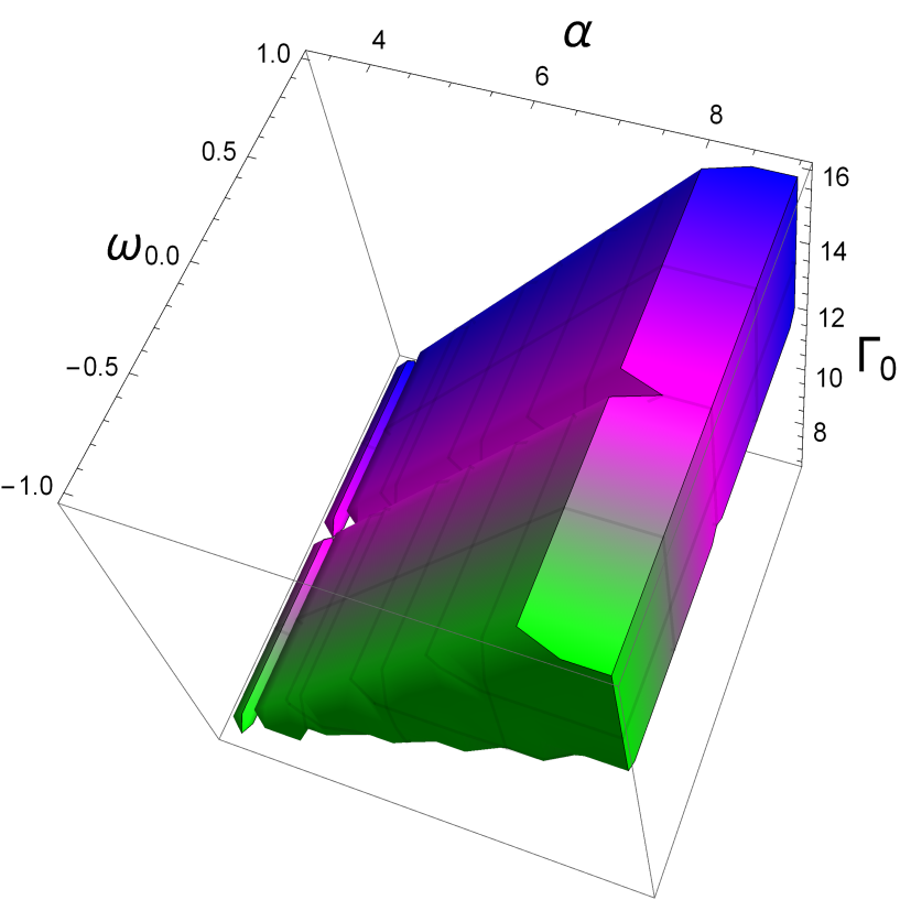
Figure 11: The figure shows the region of parametric space for complete scenario of the model parameters $\alpha$, $\omega$ and $\Gamma_{0}$.

VI Bouncing Scenario

In this section we shall study the bouncing scenario of interacting Umami Chaplygin fluid with pressureless dust via a phenomenological interaction term in the framework of particle creation mechanism. The study of bounce cosmology can be an alternative to big-bang cosmology, i.e., initial singularity. It is well known fact that inflation scenario can resolve many cosmological issues like ‘horizon problem’, ‘flatness problem’ etc. within the standard big-bang cosmology. But, it faces some phenomenological conceptual obstacles. The singularity problem is one of them, it cannot be addressed by inflationary scenario. In fact, the inflationary scenario cannot address the entire history of early evolution of the universe. For this reason, a successful theory is needed to account related to the central issues of big-bang cosmology. Bouncing cosmology is one in which the fundamental issues in cosmology like problems of big-bang singularities are addressed. In order to address the initial singularity, a huge no. of investigations have been carried out in different gravity theories [121]. In recent work, Chakraborty and Chakraborty in Ref. [122] have studied different kind of bounce in respect of Raichaudhury’s equation. For a detail study of bounce scenario in different modified gravity theories in different aspects, one may refer to the PhD thesis in Ref. [123] and references there in. Bounce scenario in some scalar field models are also investigated in context of Dynamical systems analysis in Refs. [124]. A global phase space analysis for scalar fields bouncing solutions has been reported recently in Ref.[125].

A cosmological model has no big-bang singularity initially at $t=0$ if it has the scale factor $a(t)\neq 0$ at $t=0$. Here, the universe contracts in the period $t\in(-\infty,~{}0]$ while it expands for $t\geq 0$. The following are important for the study of bouncing universe:
In non-singular bounce, first, the scale factor $a(t)$ decreases with time, i.e, contracting case ($\dot{a}(t)<0$) which implies that $H=\frac{\dot{a}}{a}<0$. Also, after some times the decreasing scale factor reaches to a critical value and finally the Hubble parameter becomes zero at the bounce point. Now the scale factor increases with time t as a result of which the Hubble parameter becomes $H=\frac{\dot{a}}{a}>0$ after the bounce. In this situation the Hubble parameter $H$ will follow the path of transition from $H<0$ to $H>0$. So, in summary, one can obtain the bounce universe in avoidance of initial singularity in the context of General Relativity after fulfilling the following requirement:

$$a(t=0)\neq 0,~{}~{}\dot{a}(t=0)=0,~{}~{}H(t=0)=0,~{}~{}\dot{H}(t=0)>0$$

Therefore, our main aim is to study the evolution of scale factor $a(t)$ and the Hubble parameter $H(t)$ for our model. In this model, particle production rate $\Gamma$ is chosen as, $\Gamma=\Gamma_{0}H$ ($\Gamma_{0}$, a constant) and the interaction term is taken as $Q=\alpha H\rho_{m}$, where the coupling parameter $\alpha$ is a dimensionless constant. Now, considering the above, we solve the Eqn.(20) for $\rho_{m}$ as follows:

$$\rho_{m}=C_{1}a^{-(\alpha-\Gamma_{0}+3)}~{}~{}~{}~{};~{}~{}C_{1}~{}~{}is~{}~{}an~{}~{}integrating~{}~{}constant.$$ (39)

Using the above explicit solution of $\rho_{m}$ in Eqn.(39), the Friedmann constraint (13) gives the solution of $\rho_{d}$ as :

$$\rho_{d}=3\left(\frac{\dot{a}}{a}\right)^{2}-C_{1}a^{-(\alpha-\Gamma_{0}+3)}$$ (40)

and the Raichaudhuri Equation in (14) will immediately provide the solution for $p_{d}$ as

$$p_{d}=\frac{\Gamma_{0}}{3}C_{1}a^{-(\alpha-\Gamma_{0}+3)}-\left\{\frac{2\ddot{a}}{a}+\left(\frac{\dot{a}}{a}\right)^{2}\right\}$$ (41)

After putting the explicit form of energy density (in Eqn. (40)) and the pressure (in Eqn. (41)) of Umami Chaplygin fluid, the equation of state of the fluid given in Eqn. (16) will give the second order differential equation for the scale factor $a(t)$ as follows:

$$\frac{2a\ddot{a}+\left(\dot{a}\right)^{2}+\frac{a^{\alpha+5}\left|A\right|\left|\omega\right|\left(C_{1}a^{\Gamma_{0}}-3a^{\alpha+1}\left(\dot{a}\right)^{2}\right)}{a^{2\alpha+6}\left|A\right|+\left|\omega\right|\left(C_{1}a^{\Gamma_{0}}-3a^{\alpha+1}\left(\dot{a}\right)^{2}\right)^{2}}}{a^{2}}-\frac{1}{3}C_{1}\Gamma_{0}a^{-\alpha+\Gamma_{0}-3}=0$$ (42)

Due to complicated form of the non-linear differential equation (42), it is very hard to solve analytically. By proper choice of initial condition, we shall solve the differential equation numerically for $a(t)$ and $H(t)$ showing in the fig. (12). From the figure we obtain a non-singular bounce scenario. This scenario consists of the following behavior of scale factor $a(t)$ and the Hubble parameter $H(t)$. A contracting phase is occurred (see in sub-fig. (12)) in pre bounce phase when $\dot{a}(t)<0$ and $H(t)=\frac{\dot{a}}{a}<0$ which is followed by a smoothly non-singular bounce point where $\dot{a}=0$, i.e., $H=0$ and the co-ordinate of the bounce point is $(a=1,~{}t=0)$ shown in the sub-fig.(12). Finally, it goes to the post-bounce expanding phase where $\dot{a}>0$ (see in sub-fig. (12)) and consequently, $H>0$ (see in sub-fig.(12)).

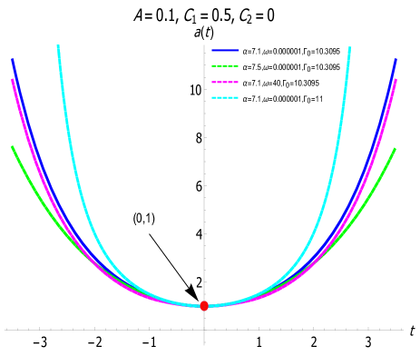
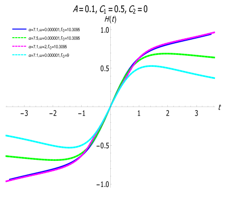
Figure 12: The figure shows the bouncing behavior of evolution of scale factor a(t) (left panel) and Hubble parameter $H(t)$ (right panel) with respect to the cosmic time t for different parameters values. $C_{1}$ and $C_{2}$ are integrating constants. In sub-figure 12 the point with red dot refers to the bouncing point.

VII Concluding remarks

We have investigated an interacting Umami Chaplygin gas in the framework of homogeneous, isotropic and spatially flat FLRW universe where gravitational induced particle creation is allowed. In this mechanism, the cosmological matter is assumed to be created irreversibly from the geometry of space-time. We have considered the universe as an open thermodynamical model of a specific volume $V$ containing $N$ number of particles. The dissipative effect in the open system is also considered, as a result of which the number of particles is not conserved in the system. In this formalism, the matter creation rate is included in energy-momentum tensor and reinterpreted the conservation laws. The created matter is assumed to be pressureless dark matter and a suitable choice of production rate ($\Gamma$) is considered as a linear function of Hubble parameter $\Gamma\propto H$ and the matter creation pressure is related to creation rate.

From a phenomenological point of view and for mathematical simplicity, we introduced an interaction term between the DE (represented by Umami Chaplygin gas) and DM (taken as pressure-less dust). Cosmological dynamics of this model is studied in the context of dynamical systems analysis.

For this, first, the cosmological evolution equations have been converted into a system of ordinary differential equations by assuming suitable choices of dimensionless variables defined in (22). We, then obtained a two-dimensional autonomous system of ordinary differential equations for our model. Critical points have been extracted from the autonomous system. The critical points and the corresponding physical parameters are displayed in the table (1). The nature of critical points is found by perturbing the system around the critical points. The eigenvalues of linearized Jacobian matrix for the critical points are presented in the table (2). The conditions for stability for each critical points have been discussed in the section IV.1 and the regions of stability in parameters space ($\alpha,~{}\Gamma_{0},~{}\omega$) for critical points are displayed in figs. (1), (2) and (3). Classical stability has also been studied (see in sect.IV.2) for the model at each critical points and identified the region of parameters at which the critical points are stable locally as well as classically.

From the dynamical analysis, it is observed that the critical points $P_{1},~{}P_{2},~{}P_{3},~{}P_{4}$ and $P_{5}$ are hyperbolic type and the linear stability theory was employed to determine their stability in phase plane. The point $P_{6}$ is normally hyperbolic set of critical points. We determined the stability by remaining non-vanishing eigenvalue and also by numerical investigation.
Some physically viable solutions are found from the analysis. We obtained the Umami Chaplygin fluid dominated solutions represented by the critical points $P_{1}$, $P_{2}$ and $P_{3}$, which depending on some parameters restrictions, can describe different phases of cosmic evolution such as the point $P_{2}$ can show the cosmological dynamics at late phase as well as the early time of the universe. In particular, for restrictions: $|\omega|<1$ and ($\Gamma_{0}-\alpha>3$), the point describes accelerated de Sitter solution corresponding to early evolution of the universe since it is source in the phase plane. On the other hand, the point corresponds to a late-time accelerated de Sitter solution representing the present evolution of the universe for the restrictions: $|\omega|>1$ and ($\Gamma_{0}-\alpha<3$), because the point is stable attractor in phase plane. These features are also clearly exhibited in the figure (4) and are analyzed in the previous section. Next, the critical point $P_{3}$ is also relevant in late-time evolution of the universe. Depending on parameters, it can describe late-time accelerated universe attracted in quintessence era. But, it cannot solve the coincidence problem since $\Omega_{d}=1$. Finally, the point $P_{1}$ can describe the dust dominated decelerating universe corresponding to transient phase for $\Gamma_{0}<\alpha$.

Cosmological viable solutions are also achieved by the DE(Umami Chaplygin gas)-DM scaling solutions $P_{4}$, $P_{5}$, and $P_{6}$. The DE and DM scale similarly in their evolution. This property explore the possibility to solve the coincidence problem (since $0<\Omega_{d}<1$). The point $P_{4}$ has interesting nature in the late time dynamics of the universe. On some parameters restrictions, it behaves like a late-time accelerated attractor in phantom regime which is in agreement with observations. This is confirmed in the figure (10). Another scaling solution $P_{5}$ shows exciting nature in its evolution. It corresponds to an accelerated scaling attractor at late-time attracted in quintessence era solving coincidence problem. In fig.(5), for $\alpha=0.2,~{}\omega=0.57,~{}\Gamma_{0}=2$ the point corresponds to the universe’s evolution yielding $\Omega_{m}\approx 0.31,~{}\Omega_{d}\approx 0.69,~{}\omega_{eff}\approx-0.6,~{}q\approx-0.4$. This phenomenon is in agreement with present observation where the Umami Chaplygin gas (as DE) behaves as quintessence fluid. This solution can solve the coincidence problem. Finally, the scaling solution, namely, the normally hyperbolic set $P_{6}$ can represent the stable attractor in late phase of the universe which is plotted in fig. (7). In particular, for $x_{c}=1$, the solution can mimic the accelerated de Sitter expansion corresponding to late-phase or at early phase of the universe. These scenarios are presented in the figs. (9) and (8).

We can summarize the results in the following: Our analysis provides some critical points exhibiting the early expansion of the universe as well as late acceleration of the universe by achieving the de Sitter solutions in phase plane. Some of points correspond to scaling attractors alleviating the coincidence problem. These scenarios are also favoured by observational data. Dust dominated decelerated intermediate phase of the universe is also achieved by some points. A numerical investigation is shown in fig.(6) which shows cosmologically viable solutions, trajectory is identified connecting a matter dominated critical point to DE dominated era achieved by scaling solutions and the cosmic evolution of relevant quantities is in agreement with observations. Beside these, we obtained a region of parameters space: [$\omega\in(-1,~{}1),~{}\omega\neq 0$ and $3+\alpha<\Gamma_{0}<2\alpha$, where $\alpha>3$] (see in fig. (11)) in which a series of critical points $P_{2}\longrightarrow P_{3}\longrightarrow P_{4}$ (in fig. 10) representing cosmologically interesting solutions, where a clear trajectory is identified connecting an early inflationary phase (represented by $P_{2}$) to a late-time DE dominated solution (described by $P_{4}$) through a matter dominated era (described by $P_{3}$). The plots (in fig.10) of physically relevant quantities ($\omega_{eff},~{}q$) prove this statement. The figure shows the numerical solution describing the cosmological evolution history of the universe where $\omega_{eff}$ evolves starting from an inflationary phase (i.e., $\omega_{eff}=-1$), passing through a sufficiently long amount of time in a matter era ($\omega_{eff}\approx 0$) and finally being attracted by late-time dark energy accelerated phase (i.e., $\omega_{eff}<-1$). A phantom crossing behaviour is also achieved in this scenario. Therefore, one can conclude that a unified cosmic evolution is achieved within this cosmological model and this statement validates the figures 10, 10 and 10. One final remark of our study is that a non-singular bouncing universe is also achieved for this model investigated numerically in fig.(12).

References

- [1] A. G. Riess et al. [Supernova Search Team Collaboration], “Observational evidence from supernovae for an accelerating universe and a cosmological constant,” Astron. J. 116 (1998) 1009, (arXiv:astro-ph/9805201).
- [2] S. Perlmutter et al., [Supernova Cosmology Project Collaboration], “Measurements of Omega and Lambda from 42 high redshift supernovae,” Astrophys. J. 517 (1999) 565, (arXiv:astro-ph/9812133).
- [3] E. Komatsu et al., Astrophys. J. Suppl. Ser. 192 (2011) 18.
- [4] A. G. Sanchez et al., Mon. Not. R. Astron. Soc. 425 (2012) 415.
- [5] P. A. R. Ade et al. [Planck Collaboration], “Planck 2013 results. XVI. Cosmological parameters,” Astron. Astrophys. 571, A16 (2014) (arXiv:1303.5076 [astro-ph.CO]).
- [6] P. A. R. Ade et al., “Planck 2015 results. XIII. Cosmological parameters”, Astron. Astrophys. 594, A13 (2016) (arXiv:1502.01589 [astro-ph.CO]).
- [7] S.M.Carroll, W.H.Press, E.L. Turner , Ann. Rev. Astron. Astrophys. 30 (1992) 499.
- [8] V.Sahni, A.A.Starobinsky , Int. J.Mod. D 9 (2000) 373.
- [9] P.J.E.Peebles, B. Ratra , Rev. Mod.Phys. 75 (2003) 559.
- [10] A.Kamenschick, U.Moschella, V.Pasquier , Phys. Lett. B. 511 (2001) 265.
- [11] B. Pourhassan, E. O. Kahya , Adv. High Energy Phys. 2014 (2014) 231452.
- [12] M. C. Bento, O. Bertolami, A.A.Sen, Phys. Rev. D 66 (2002) 043507.
- [13] V. Gorini, A. Kamenschik, U. Moschella, Phys. Rev. D 67 (2003) 063509; P.T.Silva, O.Bertolami, arXiv:astro-ph/0303353; L.Amendola, F.Finelli, C.Burigana, D.Carturan, J. Cosmol. Astropart. Phys. 0307 (2003) 005; B.R.Dinda, S.Kumar, A.A.Sen, Phys. Rev. D 90 (2014) 083515; M.R.Setare, Phys. Lett. B 648 (2007) 329; S.Li, Y.Ma,Y.Chen, Int. J. Mod. D 18 (2009) 1785; T. Multamaki, M.Maner, E.Gaztanaga, Phys. Rev. D 69 (2004) 023004; S. Chakraborty, S.Guha, Gen. Relativ. Gravit 51 (2019) 158.
- [14] R. Lazkoz, M. O. Banos, V. Salzano, Phys. Dark. Universe 24 (2019) 100279.
- [15] S. Kr. Biswas, A. Biswas Eur. Phys. J. C 81 (2021) 356.
- [16] Planck Collaboration (N. Aghanim et al.), Astron. Astrophys. 641 (2020) A6 [doi:10.1051/0004-6361/201833910]
- [17] L. Amendola, Phys. Rev. D 62 (2000) 043511 (arXiv:astro-ph/9908023).
- [18] D. Tocchini-Valentini and L. Amendola, Phys. Rev. D 65 (2002) 063508, (arXiv:astro-ph/0108143).
- [19] L. Amendola and C. Quercellini, Phys. Rev. D 68 (2003) 023514, (arXiv:astro-ph/0303228).
- [20] S. del Campo, R. Herrera and D. Pav´on, Phys. Rev. D 78 (2008) 021302, (arXiv:0806.2116 [astro-ph]).
- [21] S. del Campo, R. Herrera and D. Pav´on, J. Cosmol. Astropart. Phys. 0901 (2009) 020, (arXiv:0812.2210 [gr-qc]).
- [22] Y. L. Bolotin, A. Kostenko, O. A. Lemets and D. A. Yerokhin, Int. J. Mod. Phys. D 24 (2015) no.03, 1530007, (arXiv: 1310.0085 [astro-ph.CO]).
- [23] A. A. Costa, X. D. Xu, B. Wang, E. G. M. Ferreira and E. Abdalla, Phys. Rev. D 89 (2014) no.10, 103531, (arXiv:1311.7380 [astro-ph.CO]).
- [24] M. Khurshudyan and R. Myrzakulov, Eur. Phys. J. C 77 (2017) no.2, 65, (arXiv:1509.02263 [gr-qc]).
- [25] N. Tamanini, Phys. Rev. D 92 (2015) no.4, 043524, (arXiv: 1504.07397 [gr-qc]).
- [26] T. Harko and F. S. N. Lobo, Phys. Rev. D 87 (2013) no.4, 044018, (arXiv:1210.3617 [gr-qc]).
- [27] B. Wang, E. Abdalla, F. Atrio-Barandela and D. Pavon, Rept. Prog. Phys. 79 (2016) no.9, 096901, (arXiv:1603.08299 [astro-ph.CO]).
- [28] E. J. Copeland, A. R. Liddle and D. Wands, Phys. Rev. D 57 (1998) 4686, (arXiv:gr-qc/9711068).
- [29] J. M. Aguirregabiria, and R. Lazkoz, Phys. Rev. D 69 (2004) 123502, (arXiv:hep-th/0402190).
- [30] R. Lazkoz, G. Leon and I. Quiros, Phys. Lett. B 649 (2007) 103, (arXiv:astro-ph/0701353).
- [31] W. Fang, Y. Li, K. Zhang, and H. Qing Lu, Class. Quant. Grav. 26 (2009) 155005, (arXiv:0810.4193 [hep-th]).
- [32] G. Leon, Class. Quant. Grav. 26 (2009) 035008, ( arXiv:0812.1013 [gr-qc]).
- [33] G. Leon, P. Silveira and C. R. Fadragas, Phase-space of flat Friedmann-Robertson-Walker models with both a scalar field coupled to matter and radiation, (arXiv: 1009.0689 [gr-qc]).
- [34] S. D. Odintsov and V. K. Oikonomou, Phys. Rev. D 98 (2018) 024013, (arXiv:1806.07295 [gr-qc]).
- [35] S. D. Odintsov and V. K. Oikonomou, Phys. Rev. D 97 (2018) 124042, (arXiv:1806.01588 [gr-qc]).
- [36] S. Bahamonde, C. G. Boehmer, S. Carloni, E. J. Copeland, W. Fang and N. Tamanini, Phys. Rept. 775-777 (2018) 1-122 (arXiv:1712.03107 [gr-qc]).
- [37] R. C. Nunes, S. Pan, Mon. Not. Roy. Asron. Soc. 459 (2016) 673.
- [38] E. Di Valentino, A. Melchiorri, O. Mena, Phys. Rev. D 96 (2017) 043503, [doi:10.1103/PhysRevD.96.043503]
- [39] S. Kumar and R. C. Nunes, Phys. Rev. D 96 (2017) 103511, [doi:10.1103/PhysRevD.96.103511].
- [40] W. Yang, A. Mukherjee, E. Di Valentino, and S. Pan, Phys. Rev. D 98 (2018) 123527, [doi:10.1103/PhysRevD.98.123527].
- [41] W. Yang, S. Pan, E. Di Valentino, R. C. Nunes, S. Vagnozzi, D. F. Mota, JCAP 09 (2018) 019, (arXiv:1805.08252v3 [astro-ph.CO]).
- [42] E. Di Valentino, A. Melchiorri, O. Mena, S. Vagnozzid, Physics of the Dark Universe 30 (2020) 100666, [doi:10.1016/j.dark.2020.100666]
- [43] M. Lucca and D. C. Hooper, Phys. Rev. D 102 (2020) 123502, [doi:10.1103/PhysRevD.102.123502]
- [44] S. Kumar, Physics of the Dark Universe 33 (2021) 100862, [doi:10.1016/j.dark.2021.100862].
- [45] E. Di Valentino, O. Mena, S. Pan, L. Visinelli, W. Yang, A. Melchiorri, D. F. Mota, A. G. Riess, J. Silk, Class. Quantum Grav. 38 (2021) 153001, [ doi:10.1088/1361-6382/ac086d].
- [46] L. A. Anchordoqui, E. Di Valentino, S. Pan, W. Yang, Physics of the Dark Universe, 32 (2021) 28, [doi:10.1016/j.jheap.2021.08.001].
- [47] F. Renzi, N. B. Hogg, W. Giarè, Monthly Notices of the Royal Astronomical Society 513 (2022) 4004 [https://doi.org/10.1093/mnras/stac1030]
- [48] Ö. Akarsu, S. Kumar, E. Özülker, and J. A. Vazquez, Phys. Rev. D 104 (2021) 123512, [doi:10.1103/PhysRevD.104.123512]
- [49] A. Theodoropoulos, L. Perivolaropoulos, Universe 7 (2021) 300, [doi:10.3390/universe7080300]
- [50] S. Vagnozzi, Phys. Rev. D 102 (2020) 023518, (arXiv:1907.07569 [astro-ph.CO]).
- [51] L. Visinelli, S. Vagnozzi, U. Danielsson, Symmetry 11 (2019) 1035, (arXiv:1907.07953 [astro-ph.CO]).
- [52] E. Di Valentino, A. Melchiorri, O. Mena, and S. Vagnozzi, Phys. Rev. D 101 (2020) 063502, (arXiv:1910.09853 [astro-ph.CO]).
- [53] E. Di Valentino, A. Melchiorri, O. Mena, and S. Vagnozzi, Phys. Rev. D 102 (2020) 043517, (arXiv:1911.04520 [astro-ph.CO]).
- [54] S. Vagnozzi, L. Visinelli, O. Mena, D. F. Mota, Mon. Not. Roy. Astron. Soc. 493 (2020) 1139, (arXiv:1911.12374 [gr-qc]).
- [55] S. Pan, W. Yang, A. Paliathanasis, Mon. Not. Roy. Astron. Soc. 493 (2020) 3114, (arXiv:2002.03408 [astro-ph.CO]).
- [56] W. Yang, S. Pan, E. Di Valentino, O. Mena, A. Melchiorri, JCAP 10 (2021) 008, (arXiv:2101.03129 [astro-ph.CO]).
- [57] Li-Yang Gao, Ze-Wei Zhao, She-Sheng Xue, Xin Zhang, JCAP 07 (2021) 005, (arXiv:2101.10714 [astro-ph.CO]).
- [58] M. Lucca, Dark energy-dark matter interactions as a solution to the S8 tension, (arXiv:2105.09249 [astro-ph.CO]).
- [59] R. C. Nunes, E. Di Valentino, Phys. Rev. D 104 (2021) 063529, (arXiv:2107.09151 [astro-ph.CO]).
- [60] Rui-Yun Guo, Lu Feng, Tian-Ying Yao, Xing-Yu Chen, JCAP 12 (2021) 036, (arXiv:2110.02536 [gr-qc]).
- [61] A. Spurio Mancini, A. Pourtsidou, Mon. Not. Roy. Astron. Soc. 512 (2022) L44, (arXiv:2110.07587 [astro-ph.CO]).
- [62] F. Ferlito, S. Vagnozzi, D. F. Mota, M. Baldi, Mon. Not. Roy. Astron. Soc. 512 (2022) 1885, (arXiv:2201.04528 [astro-ph.CO]).
- [63] R. C Nunes, S. Vagnozzi, S. Kumar, E. Di Valentino, O. Mena, Phys. Rev. D 105 (2022) 123506, (arXiv:2203.08093 [astro-ph.CO]).
- [64] S. Pan, W. Yang, E. Di Valentino, D. F. Mota, J. Silk, IWDM: The fate of an interacting non-cold dark matter-vacuum scenario, (arXiv:2211.11047 [astro-ph.CO]).
- [65] S. Pan, J. de. Haro, A. Paliathanasis, and R. Jan. Slagter, Mon. Not. R. Astron. Soc. 460(2) (2016) 1445, (arXiv:1601.03955 [gr-qc]).
- [66] A. G. Riess, S. Casertano, W. Yuan, L. M. Macri, D. Scolnic, ApJ 876 (2019) 85, [doi:10.3847/1538-4357/ab1422].
- [67] A. Pourtsidou and T. Tram, Phys. Rev. D 94 (2016) 043518, [doi:10.1103/PhysRevD.94.043518].
- [68] Rui An et al., JCAP 02 (2018) 038, [doi:10.1088/1475- 7516/2018/02/038].
- [69] S. Kumar, R. C. Nunes, S. Kumar Yadav, Eur. Phys. J. C 79 (2019) 576, [doi:10.1140/epjc/s10052-019-7087-7].
- [70] J.C.N. de Araujo, A. De Felice, S. Kumar, and R. C. Nunes, Phys. Rev. D 104 (2021) 104057, [doi:10.1103/PhysRevD.104.104057].
- [71] F. Avila, A. Bernui, R. C Nunes, E. de Carvalho, C. P Novaes, Monthly Notices of the Royal Astronomical Society 509(2) (2022) 2994, [ https://doi.org/10.1093/mnras/stab3122].
- [72] Di Valentino et al., Astroparticle Physics, 131 (2021) 102604, [https://doi.org/10.1016/j.astropartphys.2021.102604].
- [73] S. Pan and S. Chakraborty, Int. J. Mod. Phys. D 23 (2014) 1450092, [doi:10.1142/S0218271814500928].
- [74] A. Bonilla and J. E. Castillo, Universe 4 (2018) 21, [https://doi.org/10.3390/universe4010021].
- [75] A. Bonilla Rivera and J. Enrique García-Farieta, Int. J. Mod. Phys. D 28 (2019) 1950118, [https://doi.org/10.1142/S0218271819501189].
- [76] G. Steigman, R. C. Santos, J.A.S. Lima, J. Cosmol. Astropart. Phys. 06 (2009) 033.
- [77] J.A.S. Lima, J. F. Jesus, F. A. Oliveira, J. Cosmol. Astropart. Phys. 11 (2010) 027.
- [78] J.A.S. Lima, L.L.Graef, D. Pavon, S. Basilakos, J. Cosmol. Astropart. Phys. 10 (2014) 042.
- [79] J.C. Fabris, J.A.F. Pacheco, O.F.Piattella, J. Cosmol. Astropart. Phys. 06 (2014) 038.
- [80] S. Chakraborty, S. Pan, S. Saha, (arXiv:1503.05552).
- [81] I. Prigogine, J. Geheniau, E. Gunzig, P. Nardone Proc. Natl. Acad. Sci. U.S.A. 85 (1988) 728.
- [82] I. Prigogine, J. Geheniau, E. Gunzig, P. Nardone Gen. Relativ. Gravit. 21 (1989) 767.
- [83] M.O.Calvao, J.A.S.Lima, I.Waga, Phys.. Lett. A 162 (1992) 233.
- [84] J.A.S.Lima, M.O.Calvao, I.Waga, Cosmology, Thermodynamics and Matter Creation, World Scintific, Singapore, Vol. 317 (1991).
- [85] J.A.S.Lima, A.S.Germano, Phys.. Lett. A 170 (1992) 373.
- [86] J.A.S.Lima, A.S.Germano, L.R.W. Abramo, Phys. Rev. D 53 (1996) 4287.
- [87] J.A.S.Lima, F.E.Silva, R.C.Santos, Class. Quant. Gravit. 25 (2008) 205006.
- [88] S. Basilakos, J.A.S.Lima, Phys. Rev. D 82 (2010) 023504.
- [89] E. Schrodinger, Physica(Amsterdam) 6 (1939) 899.
- [90] L.Parker, Phys. Rev. Lett. 21 (1968) 562; Phys. Rev. 183 (1969) 1057; Phys. Rev. D 3 (1971) 5346; L. H. Ford, L.Parker, Phys. Rev. D 16 (1977) 245; N.D.Birrell, C.P.W. Davies, Quantum Fields in Curved Space (Cambridge University Press, Cambridge, England, 1984) 21 (1968); J. Phys. A 13 (1980) 2109.
- [91] S. Chakraborty, S. Pan, S. Saha, Phys. Lett. B. 738 (2014) 424.
- [92] R. C. Nunes, D. Pavon, Phys. Rev. D 91 (2015) 063526.
- [93] R. C. Nunes, Int. J. Mod. Phys. D 25 (2016) 1650067.
- [94] S. Pan, S. Chakraborty, Adv. High Energy Phys. 2015 (2015) 654025.
- [95] L.R.W. Abramo, J.A.S.Lima, Class. Quant. Grav. 13 (1996) 2953; E. Gunzig, R. Maatens, A.V.Nesteruk, Class. Quant. Grav. 15 (1998) 923.
- [96] S. Chakraborty, Phys. Lett. B 732 (2014) 81.
- [97] J.Dutta, S.Haldar, S. Chakraborty, Astrophys. Space, Sci. 361 (2016) 21.
- [98] S. Chakraborty and S. Saha, Phys. Rev. D 90 (2014) 123505.
- [99] J. de. Haro and S. Pan, Class. Quantum Grav. 33 (2016) 165007, (arXiv:1512.03100 [gr-qc]).
- [100] C. P. Singh, A. Kumar, Phys. Rev. D. 102 (2020) 123537.
- [101] S. K. Biswas, W. Khyllep, J. Dutta, S. Chakrborty, Phys. Rev. D. 95 (2017) 103009.
- [102] J.F.Jesus, F.A.Oliveira, S.Basilakos, J.A.S.Lima, Phys. Rev. D. 84 (2011) 063511.
- [103] V. H. Cardenas, M. Cruz, (arXiv:2401.16905).
- [104] R. A.C.Cipriano, T. Harko, F. S.N. Lobo, M. A.S.Pinto, J.L.Rosa, (arXiv:2310.15018).
- [105] W. Zimdahl, Phys. Rev. D 53 (1996) 5483.
- [106] W. Zimdahl, Phys. Rev. D 61 (2000) 083511.
- [107] M. O. Calvao, J. A. S. Lima, and I. Waga, Phys. Lett. A 162 (1992) 223.
- [108] J. D. Barrow, Formation and Evolution of Cosmic Strings, edited by G. Gibbons, S. W. Hawking, and T. Vachaspati (Cambridge Univ. Press, Cambridge, England, 1990, pp. 449).
- [109] J. A. S. Lima, S. Basilakos, and F. E. M. Costa, Phys. Rev. D 86 (2012) 103534 (arXiv:1205.0868).
- [110] J. P. Mimoso, and D. Pavon, Phys. Rev. D 87 (2013) 047302 (arXiv:1302.1972).
- [111] M. Khurshudyan, and R. Myrzakulov, Eur. Phys. J. C 77 65 (2017) (arXiv:1509.02263 [gr-qc]).
- [112] C. G. Boehmer, G. C.-Cabral, R. Lazkoz, R. Maartens, Phys.Rev. D 78 (2008) 023505.
- [113] X.-m Chen, Y. Gong,E.N.Saridakis, J. Cosmol.Astropart.Phys. 04 (2009) 001.
- [114] A. A. Coley, Dynamical systems and cosmology, Springer Science Business Media 291 (2013)
- [115] S. Kr. Biswas and S. Chakraborty, Gen. Rel. Grav. 47 (2015) 22 (arXiv:1502.06913 [gr-qc]).
- [116] S. Kr. Biswas and S. Chakraborty, Int. J. Mod. Phys. D. 24 (2015) no.07, 1550046.
- [117] F.Piazza, S.Tsujikawa, JCAP 0407 (2004) 004 (arXiv:hep-th/0405054).
- [118] N. Mahata, S. Chakraborty, Gen. Relt. Grav. 46 (2014) 1721 (arXiv:1312.7644 ).
- [119] J. Garriga and V. F. Mukhanov, Phys. Lett. B. 458 (1999) 219.
- [120] S. Das, A. Al MAmon and M. Banerjee, Research in Astronomy and Astrophysics 18 (2018) 131 (arXiv:1805.07148 [gr-qc]).
- [121] S.M.Carroll, V. Duvvuri, M.Trodden, M.S.Turner, Phys. Rev. D 70 (2004) 043528; O.Bertolami, C.G.Boehmer, T.Harko, F.S.N.Lobo,Phys. Rev. D 75 (2007) 104016; K.Bamba, A.N.Makarenko, A.N.Myagky, S.Nojiri, S.D.Odintsov, J.Cosmol.Asyrpart, Phys. 01 (2014) 008; K.Bamba, A.N.Makarenko, A.N.Myagky, S.D.Odintsov,Phys. Lett.B 732 (2014) 349; S.Nojiri, S.D.Odintsov,Phys. Lett.B 631 (2005) 1; B.Li, J.D.Barrow, D.F.Mota,Phys. Rev. D 76 (2007) 044027; J.K.Singh, K.Bamba, R.NagpalS.K.J.Pacif,Phys. Rev. D 97 (2018) 123536; T.Harko, F.S.N.Lobo, S.Nojiri, S.D.Odintsov,Phys.Rev.D 84 (2011) 024020; A.S.Agarwal, L.Pati, S.K.Tripathy, B.Mishra,Phys.Dark Univ. 33 (2021) 100863; Y.F.Cai, S.H.Chen, J.B.Dent, S.Dutta, E.N.Saridakis ,Class.Quant.Grav. 28 (2011) 215011.
- [122] M.Chakraborty,S. Chakraborty, Modern Physics Letters A 38 (2023) No. 28n29, 2350129 (arXiv:2308.10498).
- [123] A.S.Agarwal, Ph.D thesis “Bouncing scenario and Cosmic Dynamics in Modified Theorries Gravity” (arXiv:2402.06895).
- [124] J.De-Santiago, J.L.Cervantes-Cota, D.Wands, Phys. Rev. D 87 (2013) 023502; S.Panda, M.Sharma, Astrophys. Space Sci. 361 (2016) 87.
- [125] A.S.Agarwal, S.Chakraborty, B.Mishra,J.Dutta, W.Khyllep, Eur. Phys. J.C. 84 (2024) 56.