Towards Better Statistical Understanding of Watermarking LLMs
‡Grado Department of Industrial and Systems Engineering, Virginia Tech )
Abstract
In this paper, we study the problem of watermarking large language models (LLMs). We consider the trade-off between model distortion and detection ability and formulate it as a constrained optimization problem based on the green-red algorithm of Kirchenbauer et al. (2023a). We show that the optimal solution to the optimization problem enjoys a nice analytical property which provides a better understanding and inspires the algorithm design for the watermarking process. We develop an online dual gradient ascent watermarking algorithm in light of this optimization formulation and prove its asymptotic Pareto optimality between model distortion and detection ability. Such a result guarantees an averaged increased green list probability and henceforth detection ability explicitly (in contrast to previous results). Moreover, we provide a systematic discussion on the choice of the model distortion metrics for the watermarking problem. We justify our choice of KL divergence and present issues with the existing criteria of “distortion-free” and perplexity. Finally, we empirically evaluate our algorithms on extensive datasets against benchmark algorithms.
1 Introduction
As the ability of large language models (LLMs) evolves rapidly, their applications have gradually touched every corner of our daily lives. However, these fast-developing tools raise concerns about the abuse of LLMs. The misuse of LLMs could harm human society in ways such as launching bots on social media, creating fake news and content, and cheating on writing school essays. The overwhelming synthetic data created by the LLMs rather than real humans is also dragging down the efforts to improve the LLMs themselves: the synthetic data pollutes the data pool and should be detected and removed to create a high-quality dataset before training (Radford et al., 2023). Numerous attempts have been made to make the detection possible which can mainly be classified into two categories: post hoc detection that does not modify the language model and the watermarking that changes the output to encode information in the content.
Post hoc detection aims to train models that directly label the texts without monitoring the generation process. Although post hoc detections do not require access to modify the output of LLMs, they do make use of statistical features such as the internal activations of the LLMs. For example, when being inspected by another LLM, the statistical properties of machine-generated texts deviate from the human-generated ones in some aspects such as the distributions of token log-likelihoods (Gehrmann et al., 2019; Ippolito et al., 2019; Zellers et al., 2019; Solaiman et al., 2019; Tian, 2023; Mitchell et al., 2023). However, post hoc ways usually rely on the fundamental assumption that machine-generated texts statistically deviate from human-generated texts, which could be challenged in two ways. The first threat is that LLMs can mimic humans better and better as time moves on, which will lead to a situation where LLMs are becoming more and more statistically indistinguishable from humans (Sadasivan et al., 2023). Although the detection is possible when LLMs are still imperfect in learning the distributions of human-generated texts (Chakraborty et al., 2023), such a cat-and-mouse game makes the detection less reliable with new models. Another drawback is that there might not be a universal statistical property of human speech across different groups of people. For instance, Liang et al. (2023) points out that GPT detectors are biased against non-native speakers as their word choices are statistically different from the ones of native speakers.
It has reached a consensus that the usage of LLMs should be regulated and tech companies have agreed to add restrictions on the LLMs (Paul et al., 2023), the watermarking scheme has become not only a widely discussed topic academically (Aaronson, 2023; Christ et al., 2023; Kirchenbauer et al., 2023a; Sadasivan et al., 2023) but also an important and feasible solution in practice. Watermarking as one kind of steganography can be divided into two cases: the ones that directly encode the output and those that twist the generation process of the language models. The former way is more traditional and the methods used can be traced back to ancient steganography to encode arbitrary information into a text. Early efforts to watermark natural language include Atallah et al. (2001, 2002); Chiang et al. (2004); Topkara et al. (2006); Meral et al. (2009); Venugopal et al. (2011). As the transformer-based language models (Vaswani et al., 2017) have been widely adopted, the nature of the next-token-prediction generating process enables the researchers to develop improved watermarking methods by monitoring/utilizing the next-token distribution. Existing methods (Aaronson, 2023; Christ et al., 2023; Kuditipudi et al., 2023; Kirchenbauer et al., 2023a; Zhao et al., 2023; Fernandez et al., 2023) mainly distort the distribution via a (sequence of) random variable(s) called key(s), and at the test phase, the detector could use the key(s) to examine the statistical properties of the texts. In short, watermarking algorithms intentionally twist the distribution of machine-generated texts to some extent and obtain a certain level of detection ability.
While watermarking algorithms such as Kirchenbauer et al. (2023a) have gained impressive empirical performance, there is no consensus on analyzing the trade-off between the model distortion and the detection ability; and there is also a lack of theoretical understanding of its success. For example, almost all theoretical analyses show how to achieve a detectable watermark up to some standard (Aaronson, 2023; Kirchenbauer et al., 2023a). But few characterize the price paid to obtain such a watermark – there are no common criteria to define the model distortion. For instance, Aaronson (2023); Kuditipudi et al. (2023) argue that the so-called “distortion-free” criteria should be considered when evaluating different watermarking algorithms, and suggest the model distortion unnecessary. Even for the models that explicitly twist the model, the hyperparameter that controls the twist extent is still chosen in a heuristic way (Kirchenbauer et al., 2023a). Another important matter is which measurement of model distortion should be used: current empirical validation mostly uses the difference of log-perplexity to measure the statistical distortion of the model (Kirchenbauer et al., 2023a) which is later analyzed by Wouters (2023), while Zhao et al. (2023) use the Kullback-Leibler divergence to measure the model distortion. In this paper, we try to give a better understanding of the watermarking algorithms by answering the following questions: Statistically, what is the minimal price for the (soft) watermarking algorithm to attain a certain level of detection ability? Furthermore, what should be considered a good measurement for the price? In summary, we address our main contributions as follows:
-
•
In Section 2, we study the statistical price paid when applying a generalized version of the soft watermarking scheme introduced in Kirchenbauer et al. (2023a). We formulate the trade-off between the model distortion and the detection ability as a constrained optimization problem that minimizes the Kullback-Leibler divergence of the watermarked model towards the original language model subject to lower bounds on the average increased green list probability (as a proxy for the detection ability). We curve the trade-off and develop an online optimization watermarking algorithm (Algorithm 2) as an asymptotic Pareto optimum under mild assumptions (Assumption 2.7) as is shown in Theorem 2.8.
-
•
In Section 3, we justify our choice of Kullback-Leibler divergence as the model distortion. We first show that any watermarked model close to the original model in the sense of KL divergence is hardly detectable via an information-theoretic lower bound (Proposition 3.1). We also show in Proposition 3.5 that the so-called “distortion-free” criterion focuses on “the distance of the expected model from the original one” rather than “the expected distance of the model from the original one”. Such two results suggest that the marginal distortion-free criterion should be reconsidered carefully and used cautiously. Later, we justify the choice of KL divergence against the difference of log-perplexity, where the latter could be smaller than zero under distortion.
-
•
In Section 4, we give some further analyses of our proposed algorithm. We develop both types of error rate guarantees over a -test, and discuss the robustness under adversarial attacks. In Section 5, we present numerical experiments. First, we compare our main algorithm Dual Gradient Ascent (Algorithm 2, abbreviated as DualGA) with existing algorithms on benchmark datasets, validating that it achieves the optimal trade-off between the model distortion and the detection ability and ensures the detectable watermark individually for every prompt. As a side result, we find that the text repetition issue encountered in existing hashing-based algorithms Kirchenbauer et al. (2023a); Aaronson (2023) is real-time detectable by monitoring DualGA’s dual variable. We also evaluate the robustness under attacks of our algorithms.
1.1 Related Literature
Watermarking Natural Languages.
Unlike the computer vision tasks where the underlying data is continuous, watermarking natural languages is deemed more difficult due to its discrete nature (Johnson et al., 2001). Traditional watermarking schemes try to transform the text into a whole new text to encode information, such as syntactic structure restructuring (Atallah et al., 2001), paraphrasing (Atallah et al., 2002), semantic substitution (Chiang et al., 2004), synonym substitution (Topkara et al., 2006), morphosyntactic alterations (Meral et al., 2009), and so on. Recent advancements in modern language models such as Transformer (Vaswani et al., 2017) enable researchers to construct new approaches based on monitoring the token generation. Aaronson (2023); Christ et al. (2023) propose an exponential minimum sampling algorithm that maintains the marginal distribution per token the same. When generating the -th token, they use the previously observed tokens as a seed for the pseudo-random function to generate a sequence of uniformly distributed random variables over for each , and select the token to minimize . By showing that the marginal distribution of each token is identical to the original distribution when averaged across the whole space of , the authors argue that such a property is desirable when conducting watermarking. Kuditipudi et al. (2023) later derive a watermarking scheme by assuming a sequence of secret keys so that each token can be uniquely assigned a pseudo-random function, resulting in a more robust watermarking at the cost of higher requirements of sharing the secret keys. Kirchenbauer et al. (2023a) develop a soft watermarking scheme based on pseudo-randomly dividing the vocabulary into a red list and a green list and increasing the probabilities in the green list. Zhao et al. (2023) propose fitting the red/green list across the whole sequence, leading to a provably more robust watermarking in comparison to the original one in Kirchenbauer et al. (2023a). Fernandez et al. (2023) point out that the -score test used in previous research (Kirchenbauer et al., 2023a) relies on a fundamental assumption of i.i.d. tokens, which may not hold in some cases, leading to an underestimated false positive rate. Wouters (2023) curves the Pareto optimum of the difference of the green list probability against the difference of the log-perplexity, arguing that the optimal strategy is to apply no watermarking at all when the expected change of log-perplexity is greater than some threshold while applying the hard watermarking in the opposite cases. While our Pareto optimum result measured by the KL divergence suggests that one should set the strength of the watermarking equal across the whole sequence, the proposal by Wouters (2023) is optimized against the difference of log-perplexity, which could be even negative and should not be regarded as a good measurement of distortion for the watermarking problem (See Section 3).
Post Hoc Detection.
The difference between the statistical properties of machine-generated texts and human-generated texts has been noticed for a long time, and researchers are making various attempts to distinguish the machine-generated texts using those features. For instance, Gehrmann et al. (2019) build a model named GLTR to use the information of the histograms of the log-likelihoods to detect machine-generated texts. Solaiman et al. (2019) make a simpler proposal by inspecting the total log-likelihood of the whole sequence. Researchers also attempt to use another language model to distinguish the texts: Ippolito et al. (2019) employ a fine-tuned BERT (Devlin et al., 2018) to classify the texts; Zellers et al. (2019) train a model called Grover to generate texts given titles and use the Grover model itself to detect the texts. A more recent example is Tian (2023) which detects the abnormally low variation in perplexity when evaluated by corresponding LLMs. Mitchell et al. (2023) observe that the outputs of LLMs tend to stay in the negative curvature regions of the log-likelihood functions and derive a classifier based on that observation.
Possibility/Impossibility Results.
There are also some debates on whether the detection of machine-generated texts is possible. Sadasivan et al. (2023) prove that if the total variation distance (denoted by ) between the language model’s distribution and the human’s language distribution vanishes, then any detector cannot get a result better than a random decision with respect to AUROC. Their impossibility result shares the same spirit of Le Cam’s method with our Proposition 3.1, which could also be regarded as another proof supporting the argument that no detection ability could be obtained without model distortion. Later, Chakraborty et al. (2023) mitigates the impossibility result by showing the term degrades exponentially fast as the number of tokens increases under the i.i.d. assumption. This implies the possibility of detection by increasing the sequence length under the circumstances that the language model deviates from humans by only a small margin per token. However, their result involving the total variation distance requires the unnatural i.i.d. assumption over the distribution per token. In contrast, our Proposition 2.3 decomposes the joint KL divergence token-wise without any specifying assumption, supporting the natural choice of the KL divergence as model distortion measurement.
1.2 Model Setup
Language models (LMs) describe the probabilities of a sequence of words that appear in a sentence. The currently mainstream LMs (Radford et al., 2019; Brown et al., 2020) work in an autoregressive manner by predicting the next token based on a given prompt and all previously observed tokens. Mathematically, an LM is a function that treats both a prompt and previous tokens as context (abbreviated as ) and maps the context to a probability vector as a prediction for the next token, where denotes the set of all probability distributions over the vocabulary . To obtain this vector , a typical LM first outputs a logit vector and applies a softmax layer to output a probability vector
Based on the distribution , the next token is sampled. The LM continues this procedure until a terminate symbol is sampled or the token sequence reaches a pre-specified maximum length . It does not hurt to assume that after receiving the first the LM continues outputting the same until the maximum length is reached. Finally, we compactly denote the whole generating process by the map , where is the prompt space. For simplicity, we omit the subscript and use to denote the whole mapping/probability model when there is no ambiguity.
We denote the marginal distribution of that generates the first tokens by and the distribution of the -th token conditioned on the previous tokens by .
The watermarking of LMs refers to a procedure that develops a watermarked language model accompanied by a detection algorithm. Ideally, the watermarked LM behaves closely to the original LM, and the detection algorithm can predict accurately whether the generated sentence is from the watermarked LM or a human. We follow the next word prediction mechanism of the LMs and denote a watermarked model by an algorithm and a key to be a function that maps the prompt and previous tokens to another probability vector over the same vocabulary . Similar to the original LM, the watermarked LM is autoregressive and based on those probability vectors . In the following, we will use to represent the probability vectors of watermarked models and (sometimes) omit the superscript for notation simplicity. A detection procedure receives the detection key and a token sequence as inputs and then gives a binary output as a prediction of whether the token sequence is generated from the watermarked LM, i.e., generated by (1 for yes and 0 for no). Naturally, one can define the two types of errors as follows:
Here is the type I error that describes the probability of predicting a normal sequence as generated by the (watermarked) LM. Precisely, the conditional part requires that the sequence is generated by , which can be based on a human, the unwatermarked LM, or other watermarked LMs. Also, is the type II error that describes the probability of predicting an LM-generated sequence as written by a human. We remark that the two errors are affected by both the watermarking procedure/algorithm and the detection algorithm.
2 Trade-off between Model Distortion and Detection Ability
The two natural desiderata for a watermarking algorithm are (i) the watermarked LM stays close to the unwatermarked LM and (ii) the watermarked text can be easily detected. We aim to provide a precise characterization of the trade-off between these two aspects. Specifically, we adopt the Kullback-Leibler divergence to measure the closeness between the two LMs (i.e., the extent of model distortion caused by watermarking) and we consider the two types of errors defined earlier as a measurement of the detection ability. To begin with, we state a generalized version of the soft watermarking scheme proposed by (Kirchenbauer et al., 2023a). The theoretical analysis, on the one hand, shows a nice structure of the algorithm, and on the other hand, reveals potential issues of the algorithm. In the next section, we discuss other watermarking algorithms and more justifications for our formulation and this red-green list-based watermarking scheme.
Algorithm 1 states a generalized soft watermarking algorithm of Kirchenbauer et al. (2023a). At each step , the algorithm randomly partitions the vocabulary into green words (with ratio ) and red words (with ratio ). The partition is based on the previous word and some random function . Then, the watermarks are inserted into the generated token sequence by increasing the probabilities of the green words. Equivalently, one adds a positive number to the logit value where is the index of the token location in the sequence, and is the word index in the vocabulary. The algorithm is stated in a more general way than Kirchenbauer et al. (2023a) in that it allows different values of while Kirchenbauer et al. (2023a) keep all of them constant, i.e., .
2.1 Constrained Optimization Formulation
The design of the algorithm increases the probability of green words appearing in the generated text, and this is the key for the detection algorithm as well. Specifically, the detection algorithm uses the key to recover the green list and the red list at each token and thus can identify whether each token in the sequence is a green or red one. If there are significantly more green words than red words over a sequence or subsequence of tokens, it will be an indicator of watermarking. In this light, the following quantity is an important indicator of the intensity of the watermarking and is closely related to the detection ability. As noted earlier, we use to denote the watermarked LM and to denote the original LM and we define the difference of the green word probability (DG) at the -th token by
| (1) |
The quantity DG measures the change in terms of the green word probability from the watermarked LM to the original LM. The larger the value of DG, the easier the generated text can be detected. We note that this quantity is a random variable that relies on the context up to token , i.e. the prompt and . In particular, the randomness comes from the partition of the green/red list which is essentially determined by the context through the hashing. However, we note that the value of DG can be fully controlled by the parameters ’s as we can see from Step 4 of Algorithm 1.
To measure the distortion of the watermarking, we consider the KL divergence defined as follows.
Definition 2.1.
For two distributions and that , the Kullback-Leibler (KL) divergence is defined by
At each step , the original LM generates the token with the distribution , and the watermarked LM generates the token with the distribution . The KL divergence between these two quantifies the extent to which the watermarking algorithm twists the -th token. As the key interest is always measuring the distance against the original LM , we abbreviate and define
We note from Algorithm 1 and the discussion above that both the difference of green word probability DG and the KL divergence can be fully controlled by the perturbs ’s under the generalized soft watermarking scheme. Thus we can rewrite both quantities as a function of ’s. That is, we denote the DG function and KL divergence by and .
Consider the following constrained optimization problem:
| (2) | ||||
where the decision variables are ’s. The right-hand side of the constraint imposes a condition that the average change of the green word probability should exceed a threshold. We will see shortly that the quantity is closely related to the detection ability. In this light, the optimization problem searches from a minimal twisted LM that achieves a certain level of detection ability. It explicitly trade-offs the two desiderata we mentioned at the beginning of this section. In particular, if we extend the domain , the optimization formulation also covers the hard watermarking scheme (Kirchenbauer et al., 2023a).
Two closely related optimization problems are
| (3) | ||||
where we restrict for all and abbreviate and as and , respectively.
| (4) | ||||
where we restrict for all and .
2.2 Analytical Properties of the Optimization Problem
In the above optimization problems, the objective function calculates the single-step KL divergence for each step and takes the summation. Indeed, we show that this also corresponds to the KL divergence between the two LMs and .
Definition 2.2.
and are two (joint) distributions of on the space . The conditional KL divergence is defined by
where the expectation is taken with respect to .
This definition gives us a tool to represent the KL divergence by the summation of single-step KL divergences as the following proposition.
Proposition 2.3.
For an LM , prompt and the watermarked LM watermarked by algorithm and key , the following decomposition holds
The left-hand side treats the two LMs as distributions over the space of sequences of tokens and measures their KL divergence. The right-hand side is decomposed into a summation where each term is the single-step conditional KL divergence. In the context of watermarking, the left-hand side captures the total amount of distortion between the original LM and the watermarked LM. And the proposition states that this total distortion is equal to the summation of token-wise distortion at each token/time step. Thus the optimization objectives are related to the proposition in the following way
To see this, the objective function is a realization of the conditional KL divergence which replaces the expectation with respect to for the first tokens with the realized sequence. In other words, the objective function for the optimization problems can be viewed an unbiased estimator of the KL divergence between the original LM and the watermarked LM.
We remark that this decomposition relationship does not hold generally for other divergence measures between two distributions. Apart from this theoretical structure, the optimization problem’s objective function also has a nice analytical form: the single-step KL divergence can be expressed closed-form in terms of ’s. This enables us to derive the following results on the optimal solution.
Proposition 2.4.
Proposition 2.5.
These two propositions state that under mild feasibility assumption, the three optimization problems (2), (3), and (4) share the same optimal solution. From an algorithm viewpoint, it means the generalization of Algorithm 1 over the original algorithm of Kirchenbauer et al. (2023a) does not bring additional benefits. We make several remarks on the implications for watermarking LLMs:
-
•
The optimal value of for the optimization problems above depends on the prompt and the original LM precisely, on the conditional distribution . For example, if we want to achieve the same level of detection ability (as the constraint of the optimization problems) for two prompts: (i) “Where is the capital of U.K.?” and (ii) “What is your favorite color?”, we should use different . For different prompts, i.e., for different , it corresponds to different optimal solution for the optimization problem. Reversely, if we use a fixed for all the generations as the original design in (Kirchenbauer et al., 2023a), it will result in a different level of detection ability and KL-divergence (from the original LM) for every prompt.
-
•
The optimization problems above can only be solved in an online fashion as it depends on the roll-out of the sequence. When we implement the watermarking algorithm, it generates the tokens one by one, and at time , we cannot foresee the future terms (from to ) in the optimization problems, which disallows solving them in an offline manner.
-
•
The proposition above states the structure of the optimal solution of the optimization problems. If we view minimizing model distortion and maximizing detection ability as a multi-objective optimization problem, one subtle point is that the fixed- version of Algorithm 1 (Kirchenbauer et al., 2023a) does not result in a Pareto optimum. This is because although the optimal remains fixed over time, it depends on the prompt, the LM, and also the green word ratio in a very complicated way. Even if we forget about the aspects of the prompt and the LM, it still requires careful coordination between the values of and to make the resultant generation on the Pareto optimal curve. This point is also verified by our numerical experiments.
These discussions motivate our development of an online algorithm for the problem which enables a uniform level of detection ability or KL-divergence across all the generations. As we will see later, it also brings other benefits to the problem.
2.3 Online Algorithm with Adaptive
Motivated by the discussions above, we develop an algorithm that not only ensures Pareto optimality (of model distortion and detection ability) but also achieves a pre-specified detection ability ( in (4)) for every generated token sequence. This requires (i) an adaptive choice of based on the prompt, the LM, and and (ii) an online implementation that learns the optimal on the fly.
Algorithm 2 gives our online algorithm for adaptive choosing . For the optimization problem (4), the optimal solution depends on (i) the prompt , (ii) the LM , and (iii) the realized generation of the tokens. Algorithm 2 uses a different over time, and ideally, it aims to have quickly. In this way, it learns the optimal online and adaptively (to the prompt). The idea of Algorithm 2 is to perform an online gradient ascent algorithm on the Lagrangian dual function for the dual variable , and uses to approximate the optimal dual variable To see this, we first introduce the Lagrangian of the optimization problem (4) as follows where the dual variable is denoted by ,
| (5) |
Denote the corresponding primal function as
and the dual function as
The following lemma states some key properties of the optimization problem (4) (which also applies to the other two optimization problems (2) and (3)).
Lemma 2.6.
-
(a)
The infimum that defines can always be achieved by setting . That is .
-
(b)
The Lagrangian dual can be decomposed token-wise: if we define and henceforth and accordingly, then (i) Part (a) also holds for each , and (ii) we have
and each is concave with .
-
(c)
Suppose the primal problem (4) is feasible. Then the strong duality holds
(6) with , where is the optimal choice of for maximizing the Lagrangian dual .
Lemma 2.6 justifies the design of Algorithm 2. The choice of in Step 4 of the algorithm serves two purposes: First, if we have converging to , then we will also have a converging to according to Part (c) of Lemma 2.6. Second, only the choice of can result in that is the gradient of and thus it ensures that the algorithm’s update of performs online gradient ascent in the dual space. The online gradient ascent procedure will converge because of the concavity of each , and this exactly dictates how we update the dual variable in Step 7 and Step 8 of Algorithm 2, where the hyper-parameter is the step size of the gradient-based updates.
The existing practice of the watermarking algorithm of (Kirchenbauer et al., 2023a) usually involves a hyper-parameter tuning procedure that finds a proper combination of and Yet we note that the procedure is conducted on a population level – once and are selected, they are applied to all the generations (for all the prompts). And we will see in the numerical experiment that this population-level choice prevents the chosen combination from staying on the Pareto optimality curve (of model distortion and detection ability). In contrast, for our algorithm, we choose adaptively for each prompt . The choice is also adaptive to the LM and also the realization of the generation.
2.4 Algorithm Analysis
Now we provide some theoretical analysis of the algorithm. The techniques are not new, and we simply aim to generate more intuitions for this watermarking algorithm.
Assumption 2.7.
We assume that
-
(a)
The green word probabilities under the original LM are i.i.d. random variables for all .
-
(b)
The optimal dual variable is bounded with a known upper bound :
Furthermore, we assume the initial and the final are within this range.
For the assumptions, Part (a) states that the green work probabilities are i.i.d., and it is much milder than to enforce all the conditional probabilities to be i.i.d. (which is quite unrealistic). We will also relax this assumption shortly. Part (b) imposes a mild condition on the boundedness of the dual optimal solution.
Remark. We note that all the three optimization problems (2), (3), and (4) are feasible if for all and . Under Assumption 2.7, both requirements are satisfied with probability at least if where hides the poly-logarithmic factors. With a moderate choice of , we can always see the optimization problems as feasible.
Theorem 2.8.
The theorem states that the expected optimality gap and the expected constraint violation are all on the order of . Note that the algorithm does not require any prior knowledge or any hyper-parameter tuning; it can adaptively fit into whatever prompt and LM and achieve a similar level of near-optimality. The proof is standard in the literature of online stochastic programming and online resource allocation (Agrawal and Devanur, 2014; Li et al., 2020).
Part (a) of Assumption 2.7 is not critical. For Algorithm 2, we can explicitly relate the sub-optimality with the extent of non-i.i.d.ness. Specifically, we can define a global non-stationarity measure (as the bandits with knapsacks literature (Liu et al., 2022))
where and denotes the average of the KL divergence and the DG function, respectively. Then the bounds in Theorem 2.8 accordingly become
In addition to the sub-optimality gap , there is an additional term related to the non-i.i.d.ness of the online process. We note that the bounds can be conservative in that in practice, we observe the algorithms perform much better than the bounds prescribe. But at least, these bounds assure that Algorithm 2 still gives a stable performance even if the i.i.d. part of Assumption 2.7 does not hold.
Remark. We note that Algorithm 2 is not the only algorithm that works for this online setting. We choose this mainly for its simplicity and nice empirical performance. As the optimization problems (3) and (4) share the same optimum and both of them can be transformed into equivalent convex programs, we can apply the algorithms in the literature of the online convex optimization with constraints to obtain theoretical guarantees without the i.i.d. assumption at all. For example, Neely and Yu (2017) proposes a virtual queue (also known as backpressure) algorithm that achieves both guarantees for regret and constraint violation without the i.i.d. assumption. Numerically, we find Algorithm 2 performs better than the backpressure algorithm and it is easier to implement as well.
3 Discussions on Model Distortion and KL Divergence
In this section, we provide more discussions on the choice of KL divergence and compare it against the other two popular criteria for the watermarking problem – perplexity and marginal distortion-free. We hope the discussion calls for more reflections on the rigorousness and properness of the measurements for the watermarked LMs’ model distortion. We believe in comparison with these two criteria, the KL divergence is a better one in quantifying the distortion of a watermarked LM and these discussions also further justify our choice of the objective function in our optimization problems.
3.1 Distortion as a Price for Watermarking
In Section 2.2, we establish a connection between the objective function of the optimization problems and the KL divergence between the original LM and the watermarked LM The following proposition further connects the two types of errors with the model distortion under the KL divergence.
Proposition 3.1.
For any prompt and any watermarking scheme , we have
In particular, when the KL divergence tends to zero, the sum of two types of errors under any detection algorithm cannot be better than a random decision.
While the above proposition seems similar to the results in Sadasivan et al. (2023); Chakraborty et al. (2023), the intuition behind it is quite different. Specifically, the existing results (Sadasivan et al., 2023; Chakraborty et al., 2023) characterize the possibility/impossibility of distinguishing AI-generated texts from humans. For the watermarking problem, the setting is quite different in that the watermarking algorithm is allowed to twist the original LM. In this sense, the KL divergence can be viewed as a minimum price for distinguishing the watermarked LM against an arbitrary distribution
The optimization problems (2), (3), and (4) all concern the minimum model distortion (the objective) to achieve a certain level of detection ability (the constraint). The above proposition further reinforces such a relationship that one has to distort the model (in terms of a positive KL divergence) to be able to distinguish the watermarked LM from all the other LMs.
3.2 Comparison with Other Criteria
The distribution distortion caused by watermarking is mainly characterized in two ways by the existing literature: (i) the distance between the marginal distributions that generate each token and (ii) the difference of expected logarithm perplexity. The former is often used in theoretical analysis (Aaronson, 2023; Christ et al., 2023; Kuditipudi et al., 2023) and the latter in empirical evaluation (Tian, 2023; Liang et al., 2023; Kirchenbauer et al., 2023a; Wouters, 2023). In this subsection, we compare the KL divergence with those two popular criteria.
3.2.1 Comparison with Log-Perplexity
The notion of perplexity (PPL) has been long used as a performance measure for evaluating language models, and it is also commonly used for the problem detecting AI-generated texts from humans (Wallach et al., 2009; Beresneva, 2016; Tian, 2023). Formally, the perplexity is defined as follows.
Definition 3.2.
For an evaluation language model , a prompt , and a token sequence , the perplexity (PPL) is defined as
In practice, the perplexity is often used taking the logarithm, resulting in the logarithm of the perplexity (LoP). Furthermore, the expected logarithm of the perplexity of a language model can be defined as
and the model distortion of is measured via the difference of the expected logarithm of the perplexity (DLoP)
A line of research (Kirchenbauer et al., 2023a; Wouters, 2023) in the watermarking field utilizes DLoP as a measurement of model distortion in the belief that the model distortion is small if the DLoP is small. In such a measurement the evaluation LM is often chosen to be the original LM or a larger LM. Despite the properness of the perplexity in other NLP tasks, its usage in evaluating model distortion in watermarking can be misleading. The reason is that it may lead to an awkward situation where one could severely twist the language model while making the perplexity even smaller. Such an intuition is formalized as follows.
Proposition 3.3.
Consider generating a fixed length of tokens with a prompt and using the same language model in evaluation so that . Suppose there is no tie in for and . Then there exists , s.t.
while
The LM can be simply constructed by a deterministic LM that always predicts the word with the largest probability under the original LM This even decreases the perplexity against the original LM but it is apparently not a good LM in that (i) it is a deterministic one and (ii) it has a positive KL-divergence from the original LM Therefore, Proposition 3.3 warns a potential issue of using the perplexity to measure the performance of a watermarked LM.
3.2.2 Comparison with Marginal Distortion-Free
Another popular criterion for defining a good watermarking algorithm is to check if the watermarked LM is marginal distortion-free (Aaronson, 2023; Christ et al., 2023; Kuditipudi et al., 2023). A watermarking algorithm is called marginal distortion-free if the average distribution of the next token prediction under the watermarked LM exactly matches the original LM, where the average is taken for the key . We formally define it as follows.
Definition 3.4.
A watermarking algorithm is called as marginally distortion-free if for any language model , the following holds for all and prompt
From this definition, we believe a rigorous name for this property should be marginally distortion-free, while the existing literature simply calls it distortion-free. Calling it distortion-free gives a misconception that the watermarking algorithm does not make or need any change to the underlying LM, which can be misleading and dangerous. One can think of this marginal distortion-free property as a property of the watermarking algorithm on the population level. Population-wise, if we aggregate the LM received by all the users (statistically, marginalizing over the users), it matches the original LM. But each user may receive one sample path of the watermarked LM which is drastically different from the original LM. A guarantee of marginally distortion-free says nothing about one user’s experience as it only concerns an averaging experience for all the users. In comparison, the KL-divergence that we study throughout our paper and in all the above optimization problems, ensure the model distortion in a sample-path manner. That is, it ensures every realization of the watermarked LM behaves closely to the original LM.
Proposition 3.5.
It holds that
The above proposition characterizes the relationship between the two measurements of model distortion. Our measurement of the KL divergence can be viewed as an upper bound of the marginal distortion of the LM (on the left-hand side). The marginal distortion-free property requires
To give some concrete examples, we provide a result on the popular exponential minimum sampling in Aaronson (2023); Christ et al. (2023); Kuditipudi et al. (2023). We show that it yields an expected KL divergence whose quantity is the same as the entropy of the original model.
Example 3.6.
To interpret this example, it means the watermarked LM (of the exponential minimum sampling algorithm) received by one user has a KL divergence towards the original LM that is as large as the entropy of the original LM. This resolves the seeming contradiction between our impossibility result in Proposition 3.1 and the existence of “distortion-free” algorithms. The marginal distortion-free criterion hides the necessary price paid for the watermarking. Such a criterion itself does not necessarily imply a practical failure, but it does not rule out those possibilities. For example, Kuditipudi et al. (2023) notice a phenomenon in practice when applying the watermarking scheme of Aaronson (2023) that the watermarked model would be easily trapped in a tautology (that is, constantly repeating the same sentence). The above proposition and example explain such an undesirable phenomenon.
4 Detection Ability and Robustness
In this section, we develop error guarantees for our algorithm/the optimization problems and discuss the robustness aspect of the algorithm.
4.1 Type I and Type II Error
When we present the optimization problems, the constraint is interpreted as a proxy for detection ability. Now we formally establish the connection between the cumulative difference in green word probability (DG) and the detection error. The result shows that such an optimization formulation and Algorithm 2 provide not only a better theoretical guarantee but also an explicit handle for controlling the individual guarantee for both types of error of the watermarked LM regardless of the received prompt in contrast to previous algorithms.
As noted in Fernandez et al. (2023), the -test used in Kirchenbauer et al. (2023a) only serves as an asymptotic approximation of the true positive rate. Thus, we follow the Beta distribution way in Fernandez et al. (2023) in practice. For theoretical simplicity, we present two types of error bounds based on setting an explicit threshold for the -score on the green token numbers. We define the -score as
| (7) |
where is defined by the count of green words from the 2-nd token to the -th token. Then we have the following bound.
Proposition 4.1.
Proposition 4.1 states that if we fix the type I error rate , the type II error rate decreases exponentially fast in terms of . Importantly, this result entails an individual control of the actual , i.e, the meet the constraint of the optimization problem for each prompt, LM, and . The requires to solve the optimization program (4) in hindsight. While this is impossible generally, our algorithm ensures the constraint is violated up to the order of . Comparatively, this logic also explains why Kirchenbauer et al. (2023a)’s heuristic and fixed choice of does not lead to any type II error rate until it has witnessed all the realized tokens; such an intuition is also shown in the original type II error analysis of Kirchenbauer et al. (2023a), which relies on the average entropy of the token sequence and cannot be guaranteed until the full sequence is generated.
![[Uncaptioned image]](/html/2403.13027/assets/x1.png) Figure 1: The scatter plot of -score v.s. realized DG for different algorithms. SRL stands for the algorithm in (Kirchenbauer et al., 2023a) and DualGA stands for our Algorithm 2 under different parameter combinations. Each point represents one generated sequence, and for each algorithm, 200 sequences are generated.
Figure 1: The scatter plot of -score v.s. realized DG for different algorithms. SRL stands for the algorithm in (Kirchenbauer et al., 2023a) and DualGA stands for our Algorithm 2 under different parameter combinations. Each point represents one generated sequence, and for each algorithm, 200 sequences are generated.
Figure 1 provides a visualization of the relationship between the realized DG and the -score. First, we observe that a larger realized DG corresponds to a larger -score which justifies the choice of using DG as the constraint of the optimization problem. Second, we observe that our algorithm, though implemented in an online fashion, meets the (offline) constraint well (that the realized DG ). Third, our adaptive choice of gives a more precise control of the realized DG and the -score. For any combination of and , the sequences generated by SRL have a quite dispersed DG and realized -score.
4.2 Robustness
The following proposition states the robustness of our watermarked algorithm. Specifically, it says how the detection ability changes under different adversarial attacks that aim to undermine the effectiveness of the watermarking algorithm.
Proposition 4.2.
Consider the following three adversarial attacks:
-
•
Deletion: One adversarially deletes a certain length of the token sequence from the sequence generated by the watermarked LM of Algorithm 2. Let the length of the deleted sequence being , and define
-
•
Insertion: One adversarially inserts a certain length of token sequence into the sequence generated by the watermarked LM of Algorithm 2. Let the inserted sequence length , and define
-
•
Edit: One adversarially edits a certain length of the token sequence generated by the watermarked LM of Algorithm 2. Let the edited sequence length , and define
The error bound in Proposition 4.1 holds for instead of and new sequence length correspondingly.
The proof of the proposition follows the same logic as that of Proposition 4.1. It implies that the watermarked text is robust against an adversarial attack up to linearly many changes to the generated text.
5 Experiments
In this section, we evaluate our Dual Gradient Ascent (DualGA) algorithm (Algorithm 2). The code for the numerical experiments is available at https://github.com/ZhongzeCai/DualGA. First, we compare the algorithm’s detection ability and model distortion extent with existing benchmarks and empirically show it achieves the optimal trade-off between these two aspects and consistently assures the detection ability across every prompt. Second, we further test the algorithm’s robustness under attacks on the watermarked texts. Third, we provide an approach for detecting the text repetition issue in hashing-based watermarking methods by monitoring DualGA’s dual variable.
5.1 Experiment Setup
To generate watermarked texts, we utilize the LLaMA-7B model (Touvron et al., 2023), leveraging the Huggingface Library (Wolf et al., 2019) for text generation and data management.
Datasets. The experiments test the algorithms in two datasets: C4 (Raffel et al., 2020) and LFQA (Fan et al., 2019). The C4 dataset is an extensive collection of English-language texts sourced from the public Common Crawl web scrape, and its “realnewslike” subset is where we extract prompt samples. Specifically, we select text data from its “text” domain, where the last tokens are taken as the baseline completion and the rest of tokens are used to construct the prompt dataset. The LFQA dataset, designed for long-form question-answering, is compiled by picking questions with their longest answers from Reddit. We directly take the questions as prompts and the best answers as baseline completions. More details about the dataset construction are provided in Appendix D.1.1.
Benchmark Algorithms. We consider the Soft Red List (SRL) watermarking algorithm proposed in Kirchenbauer et al. (2023a) (which keeps in Algorithm 1) and the Exponential Minimum Sampling (EMS) method from Aaronson (2023). For the SRL algorithm, we tune the hyper-parameter , i.e., the proportion of the green list, and the parameter , i.e., the constant perturbs added to all green list’s words. For the EMS algorithm, as suggested in Fernandez et al. (2023), we tune the generating temperature , which adjusts the logits used to generate watermarked texts. Further implementation details of these benchmark algorithms and DualGA are provided in Appendix D.1.2.
5.2 Detection Ability, Distortion, and Pareto Optimality
In this subsection, we evaluate the detection ability and distortion level of different algorithms. To test the detection ability, we control the false positive rate (FPR), i.e., the probability of predicting an unwatermarked text as watermarked, at pre-specified levels ( or ) and quantifies the detection ability by the true positive rates (TPR), i.e., the probability of successfully detecting a watermarked text. The model distortion is measured by the KL-divergence (KL) (averaged over tokens) between the watermarked and unwatermarked text distributions, as defined in Section 3. We also provide more discussions on the detection ability metrics in Appendix D.1.3.
Table 1 shows the evaluation of the detection ability (TPR) alongside the model distortion (KL). For each algorithm family we set multiple configurations, with each of them tested on two datasets with two significance levels ( and ) (with the results under more configurations deferred to Table 2 in Appendix D.2.1). Each configuration of these algorithms corresponds to a different combination of the detection ability and the model distortion. In comparison, our algorithm of DualGA exhibits a better trade-off between the two aspects; for a certain level of model distortion, our algorithm achieves a higher TPR, and conversely, for a certain level of TPR, our algorithm exhibits a smaller model distortion.
| Method | Configuration | C4 | LFQA | ||||
|---|---|---|---|---|---|---|---|
| TPR | KL | TPR | KL | ||||
| FPR | FPR | FPR | FPR | ||||
| SRL | 0.15 | 0.04 | 0.04 | 0.31 | 0.1 | 0.04 | |
| 0.49 | 0.18 | 0.07 | 0.56 | 0.22 | 0.07 | ||
| 0.22 | 0.04 | 0.05 | 0.33 | 0.11 | 0.05 | ||
| 0.99 | 0.98 | 1.3 | 1.0 | 0.98 | 1.29 | ||
| 1.0 | 1.0 | 0.7 | 1.0 | 1.0 | 0.69 | ||
| 0.96 | 0.92 | 0.39 | 0.98 | 0.96 | 0.39 | ||
| 1.0 | 0.99 | 1.69 | 1.0 | 0.98 | 1.46 | ||
| 1.0 | 0.99 | 1.07 | 0.99 | 0.99 | 0.9 | ||
| 0.99 | 0.96 | 0.62 | 0.96 | 0.94 | 0.51 | ||
| EMS | 0.44 | 0.21 | 0.65 | 0.26 | 0.16 | 0.47 | |
| 0.94 | 0.87 | 0.98 | 0.94 | 0.94 | 0.91 | ||
| 0.98 | 0.98 | 2.44 | 1.0 | 1.0 | 1.64 | ||
| DualGA | 0.9 | 0.7 | 0.15 | 0.91 | 0.72 | 0.13 | |
| 0.97 | 0.96 | 0.33 | 0.98 | 0.96 | 0.3 | ||
| 1.0 | 0.98 | 0.61 | 1.0 | 1.0 | 0.55 | ||
| 1.0 | 1.0 | 0.93 | 1.0 | 0.98 | 0.83 | ||
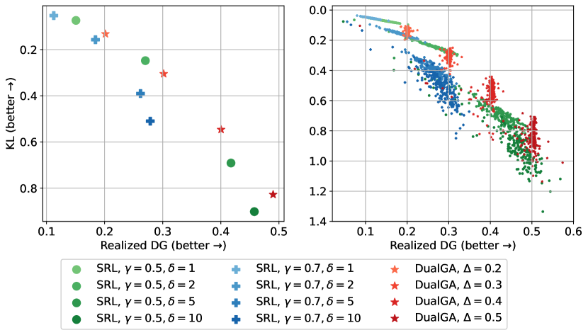
Figure 2 visualizes the trade-off between the detection ability and the model distortion. It plots the realized DG against the KL both on the population level (left) where each point represents one algorithm configuration’s averaged performance of 500 test prompts, and on the individual level (right), where each point corresponds to the outcome from a single prompt. Here, the realized DG is calculated as the realized difference in the green word probability (defined in (1) and computed by the average over for each prompt).
On the population level, Figure 2 (left) shows that our algorithm achieves a Pareto optimality in comparison with the SRL algorithm. The SRL algorithm exhibits suboptimality when the parameters and do not coordinate well (the blue points and the two green points). This reinforces the theoretical finding in Section 2.2 that the optimal choice of depends on many factors including . On the individual (prompt) level, Figure 2 (right) shows the performance of these algorithms for each prompt. For our algorithm, it exhibits a very concentrated DG level (near the target ) for different prompts. For the SRL algorithm, we can see that it attains a highly varied level of model distortion and detection ability for each prompt even under the same parameter configuration of and . Moreover, both plots in Figure 2 show that our algorithm achieves a Pareto optimality for whatever choice of the constraint budget parameter . In other words, the parameter gives a handle to balance the trade-off but does not affect the algorithm’s Pareto optimality.
Another interesting phenomenon in Figure 2 (right) is that, for our DualGA algorithm, the variation of its distortion (KL) and the realized DG exhibit a positive correlation. We note that the algorithm minimizes model distortion subject to a specific detection ability, and this suggests that prompts that are inherently more challenging to watermark (e.g., factual questions like “Where is the capital of the U.K.?”) require a greater distortion change to achieve the same level of detection abilities compared to inherently easier prompts (e.g., opinion questions like “What is your favorite color?”). For a small detection target , both types of prompts may only need some minor modification to the original response to meet the detection target and thus both allow low distortion. However, to achieve higher detection ability, more complex prompts necessitate stronger watermarking efforts, potentially skewing the correct answer or incorporating redundant tokens, whereas easier prompts allow more flexibility for embedding watermarks and thus still a small distortion. Additional results using the C4 dataset and comparisons with the EMS algorithm are provided in Appendix D.2.2.
5.3 Robustness under Attacks
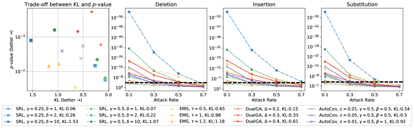
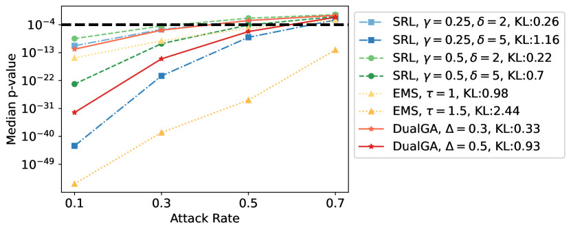
We further assess the robustness of our DualGA algorithm by considering three common types of attacks on watermarked texts: deletion, insertion, and substitution. Figure 3 shows the median -value (see Appendix D.1.3 for definition) under the deletion attack on the C4 dataset for different algorithms and varying deletion rates (proportions of deleted tokens). From the plot, the benchmark algorithms that achieve a higher level of robustness (smaller -value) than our algorithm all result in a much larger KL divergence (model distortion). For robustness analyses and more discussions under other types of attacks please refer to Appendix D.2.3.
5.4 Detection of Repetitions in Generated Text
Most (if not all) of these existing watermarking algorithms rely on hashing-based rules for generating watermarks. For example, the green word-based watermarking algorithms generate the partition of the vocabulary for each token based on a hashing-based pseudo-random function. This type of hashing-based design can cause the issue of text repetition, as empirically observed by Kuditipudi et al. (2023). Specifically, if a sequence of tokens typically appears together and the hashing code for the final token in the sequence happens to skew the vocabulary distribution significantly towards the first token, this can lead to the sampling of a repetitive chunk, creating a cyclical pattern (illustrated in Figure 4 (left)). While such cycles may emerge infrequently at the population level, their detection with the subsequent fixing is crucial to ensure quality on the individual (prompt) level. Traditional global metrics like entropy or KL-divergence are insufficient for identifying these repetitions, as they might happen only two or three times before the generating process exits the cycle.
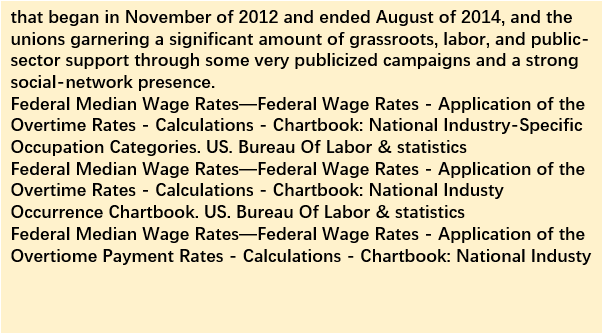
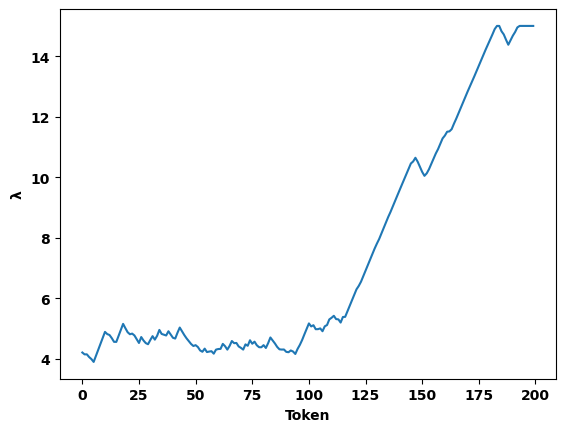
Figure 4 (right) plots the dual variables of our algorithm for the sequence generated on Figure 4 (left). We can see the dual variable significantly jumps up when the repetition starts. This phenomenon is indeed general and reasonable. The rationale is that, generally, a token sequence appearing with high certainty may pose a great challenge to the watermarking process: modest watermarking strength (smaller dual variable ) may not suffice to override the certainty inherent in selecting the subsequent word. Therefore, the algorithm needs to increase the dual variable significantly. The repetitions can be viewed as a very deterministic generation that requires increasing the dual variable. In this light, the dual variable works as a monitor for the repetition phenomenon of the watermarking process. We provide more examples in Appendix D.2.4.
References
- Aaronson (2023) Aaronson, Scott. 2023. Watermarking of large language models. URL https://simons.berkeley.edu/talks/scott-aaronson-ut-austin-openai-2023-08-17.
- Agrawal and Devanur (2014) Agrawal, Shipra, Nikhil R Devanur. 2014. Fast algorithms for online stochastic convex programming. Proceedings of the twenty-sixth annual ACM-SIAM symposium on Discrete algorithms. SIAM, 1405–1424.
- Atallah et al. (2001) Atallah, Mikhail J, Victor Raskin, Michael Crogan, Christian Hempelmann, Florian Kerschbaum, Dina Mohamed, Sanket Naik. 2001. Natural language watermarking: Design, analysis, and a proof-of-concept implementation. Information Hiding: 4th International Workshop, IH 2001 Pittsburgh, PA, USA, April 25–27, 2001 Proceedings 4. Springer, 185–200.
- Atallah et al. (2002) Atallah, Mikhail J, Victor Raskin, Christian F Hempelmann, Mercan Karahan, Radu Sion, Umut Topkara, Katrina E Triezenberg. 2002. Natural language watermarking and tamperproofing. International workshop on information hiding. Springer, 196–212.
- Beresneva (2016) Beresneva, Daria. 2016. Computer-generated text detection using machine learning: A systematic review. Natural Language Processing and Information Systems: 21st International Conference on Applications of Natural Language to Information Systems, NLDB 2016, Salford, UK, June 22-24, 2016, Proceedings 21. Springer, 421–426.
- Boyd and Vandenberghe (2004) Boyd, Stephen P, Lieven Vandenberghe. 2004. Convex optimization. Cambridge university press.
- Bretagnolle and Huber (1978) Bretagnolle, Jean, Catherine Huber. 1978. Estimation des densités: risque minimax. Séminaire de probabilités de Strasbourg 12 342–363.
- Brockwell and Davis (1986) Brockwell, Peter J, Richard A Davis. 1986. Time series: theory and methods. Springer-Verlag, Berlin, Heidelberg.
- Brown et al. (2020) Brown, Tom, Benjamin Mann, Nick Ryder, Melanie Subbiah, Jared D Kaplan, Prafulla Dhariwal, Arvind Neelakantan, Pranav Shyam, Girish Sastry, Amanda Askell, et al. 2020. Language models are few-shot learners. Advances in neural information processing systems 33 1877–1901.
- Chakraborty et al. (2023) Chakraborty, Souradip, Amrit Singh Bedi, Sicheng Zhu, Bang An, Dinesh Manocha, Furong Huang. 2023. On the possibilities of ai-generated text detection. arXiv preprint arXiv:2304.04736 .
- Chiang et al. (2004) Chiang, Yuei-Lin, Lu-Ping Chang, Wen-Tai Hsieh, Wen-Chih Chen. 2004. Natural language watermarking using semantic substitution for chinese text. Digital Watermarking: Second International Workshop, IWDW 2003, Seoul, Korea, October 20-22, 2003. Revised Papers 2. Springer, 129–140.
- Christ et al. (2023) Christ, Miranda, Sam Gunn, Or Zamir. 2023. Undetectable watermarks for language models. arXiv preprint arXiv:2306.09194 .
- Devlin et al. (2018) Devlin, Jacob, Ming-Wei Chang, Kenton Lee, Kristina Toutanova. 2018. Bert: Pre-training of deep bidirectional transformers for language understanding. arXiv preprint arXiv:1810.04805 .
- Fan et al. (2019) Fan, Angela, Yacine Jernite, Ethan Perez, David Grangier, Jason Weston, Michael Auli. 2019. Eli5: Long form question answering. arXiv preprint arXiv:1907.09190 .
- Fernandez et al. (2023) Fernandez, Pierre, Antoine Chaffin, Karim Tit, Vivien Chappelier, Teddy Furon. 2023. Three bricks to consolidate watermarks for large language models. 2023 IEEE International Workshop on Information Forensics and Security (WIFS). IEEE, 1–6.
- Gehrmann et al. (2019) Gehrmann, Sebastian, Hendrik Strobelt, Alexander M Rush. 2019. Gltr: Statistical detection and visualization of generated text. arXiv preprint arXiv:1906.04043 .
- Hoeffding (1994) Hoeffding, Wassily. 1994. Probability inequalities for sums of bounded random variables. The collected works of Wassily Hoeffding 409–426.
- Ippolito et al. (2019) Ippolito, Daphne, Daniel Duckworth, Chris Callison-Burch, Douglas Eck. 2019. Automatic detection of generated text is easiest when humans are fooled. arXiv preprint arXiv:1911.00650 .
- Johnson et al. (2001) Johnson, Neil F, Zoran Duric, Sushil Jajodia. 2001. Information hiding: steganography and watermarking-attacks and countermeasures: steganography and watermarking: attacks and countermeasures, vol. 1. Springer Science & Business Media.
- Kirchenbauer et al. (2023a) Kirchenbauer, John, Jonas Geiping, Yuxin Wen, Jonathan Katz, Ian Miers, Tom Goldstein. 2023a. A watermark for large language models. arXiv preprint arXiv:2301.10226 .
- Kirchenbauer et al. (2023b) Kirchenbauer, John, Jonas Geiping, Yuxin Wen, Manli Shu, Khalid Saifullah, Kezhi Kong, Kasun Fernando, Aniruddha Saha, Micah Goldblum, Tom Goldstein. 2023b. On the reliability of watermarks for large language models. arXiv preprint arXiv:2306.04634 .
- Kuditipudi et al. (2023) Kuditipudi, Rohith, John Thickstun, Tatsunori Hashimoto, Percy Liang. 2023. Robust distortion-free watermarks for language models. arXiv preprint arXiv:2307.15593 .
- Le Cam (2012) Le Cam, Lucien. 2012. Asymptotic methods in statistical decision theory. Springer Science & Business Media.
- Li et al. (2020) Li, Xiaocheng, Chunlin Sun, Yinyu Ye. 2020. Simple and fast algorithm for binary integer and online linear programming. Advances in Neural Information Processing Systems 33 9412–9421.
- Liang et al. (2023) Liang, Weixin, Mert Yuksekgonul, Yining Mao, Eric Wu, James Zou. 2023. Gpt detectors are biased against non-native english writers. arXiv preprint arXiv:2304.02819 .
- Liu et al. (2022) Liu, Shang, Jiashuo Jiang, Xiaocheng Li. 2022. Non-stationary bandits with knapsacks. Advances in Neural Information Processing Systems 35 16522–16532.
- Meral et al. (2009) Meral, Hasan Mesut, Bülent Sankur, A Sumru Özsoy, Tunga Güngör, Emre Sevinç. 2009. Natural language watermarking via morphosyntactic alterations. Computer Speech & Language 23(1) 107–125.
- Mitchell et al. (2023) Mitchell, Eric, Yoonho Lee, Alexander Khazatsky, Christopher D Manning, Chelsea Finn. 2023. Detectgpt: Zero-shot machine-generated text detection using probability curvature. International Conference on Machine Learning. PMLR, 24950–24962.
- Neely and Yu (2017) Neely, Michael J, Hao Yu. 2017. Online convex optimization with time-varying constraints. arXiv preprint arXiv:1702.04783 .
- Paul et al. (2023) Paul, Kari, Johana Bhuiyan, Dominic Rushe. 2023. Top tech firms commit to ai safeguards amid fears over pace of change. The Guardian URL https://www.theguardian.com/technology/2023/jul/21/ai-ethics-guidelines-google-meta-amazon.
- Polyanskiy and Wu (2014) Polyanskiy, Yury, Yihong Wu. 2014. Lecture notes on information theory. Lecture Notes for ECE563 (UIUC) and 6(2012-2016) 7.
- Radford et al. (2023) Radford, Alec, Jong Wook Kim, Tao Xu, Greg Brockman, Christine McLeavey, Ilya Sutskever. 2023. Robust speech recognition via large-scale weak supervision. International Conference on Machine Learning. PMLR, 28492–28518.
- Radford et al. (2019) Radford, Alec, Jeffrey Wu, Rewon Child, David Luan, Dario Amodei, Ilya Sutskever, et al. 2019. Language models are unsupervised multitask learners. OpenAI blog 1(8) 9.
- Raffel et al. (2020) Raffel, Colin, Noam Shazeer, Adam Roberts, Katherine Lee, Sharan Narang, Michael Matena, Yanqi Zhou, Wei Li, Peter J Liu. 2020. Exploring the limits of transfer learning with a unified text-to-text transformer. The Journal of Machine Learning Research 21(1) 5485–5551.
- Sadasivan et al. (2023) Sadasivan, Vinu Sankar, Aounon Kumar, Sriram Balasubramanian, Wenxiao Wang, Soheil Feizi. 2023. Can ai-generated text be reliably detected? arXiv preprint arXiv:2303.11156 .
- Solaiman et al. (2019) Solaiman, Irene, Miles Brundage, Jack Clark, Amanda Askell, Ariel Herbert-Voss, Jeff Wu, Alec Radford, Gretchen Krueger, Jong Wook Kim, Sarah Kreps, et al. 2019. Release strategies and the social impacts of language models. arXiv preprint arXiv:1908.09203 .
- Tian (2023) Tian, Edward. 2023. Gptzero update v1. URL https://gptzero.substack.com/p/gptzero-update-v1.
- Topkara et al. (2006) Topkara, Mercan, Giuseppe Riccardi, Dilek Hakkani-Tür, Mikhail J Atallah. 2006. Natural language watermarking: Challenges in building a practical system. Security, Steganography, and Watermarking of Multimedia Contents VIII, vol. 6072. SPIE, 106–117.
- Touvron et al. (2023) Touvron, Hugo, Thibaut Lavril, Gautier Izacard, Xavier Martinet, Marie-Anne Lachaux, Timothée Lacroix, Baptiste Rozière, Naman Goyal, Eric Hambro, Faisal Azhar, et al. 2023. Llama: Open and efficient foundation language models. arXiv preprint arXiv:2302.13971 .
- Vaswani et al. (2017) Vaswani, Ashish, Noam Shazeer, Niki Parmar, Jakob Uszkoreit, Llion Jones, Aidan N Gomez, Łukasz Kaiser, Illia Polosukhin. 2017. Attention is all you need. Advances in neural information processing systems 30.
- Venugopal et al. (2011) Venugopal, Ashish, Jakob Uszkoreit, David Talbot, Franz Josef Och, Juri Ganitkevitch. 2011. Watermarking the outputs of structured prediction with an application in statistical machine translation. Proceedings of the 2011 Conference on Empirical Methods in Natural Language Processing. 1363–1372.
- Wallach et al. (2009) Wallach, Hanna M, Iain Murray, Ruslan Salakhutdinov, David Mimno. 2009. Evaluation methods for topic models. Proceedings of the 26th annual international conference on machine learning. 1105–1112.
- Wolf et al. (2019) Wolf, Thomas, Lysandre Debut, Victor Sanh, Julien Chaumond, Clement Delangue, Anthony Moi, Pierric Cistac, Tim Rault, Rémi Louf, Morgan Funtowicz, et al. 2019. Huggingface’s transformers: State-of-the-art natural language processing. arXiv preprint arXiv:1910.03771 .
- Wouters (2023) Wouters, Bram. 2023. Optimizing watermarks for large language models. arXiv preprint arXiv:2312.17295 .
- Yellott Jr (1977) Yellott Jr, John I. 1977. The relationship between luce’s choice axiom, thurstone’s theory of comparative judgment, and the double exponential distribution. Journal of Mathematical Psychology 15(2) 109–144.
- Zellers et al. (2019) Zellers, Rowan, Ari Holtzman, Hannah Rashkin, Yonatan Bisk, Ali Farhadi, Franziska Roesner, Yejin Choi. 2019. Defending against neural fake news. Advances in neural information processing systems 32.
- Zhao et al. (2023) Zhao, Xuandong, Prabhanjan Ananth, Lei Li, Yu-Xiang Wang. 2023. Provable robust watermarking for ai-generated text. arXiv preprint arXiv:2306.17439 .
- Zinkevich (2003) Zinkevich, Martin. 2003. Online convex programming and generalized infinitesimal gradient ascent. Proceedings of the 20th international conference on machine learning (icml-03). 928–936.
Appendix A Proofs and Discussions in Section 2
A.1 Proof of Proposition 2.4
Proof.
We consider the following one-step optimization program with respect to where we omit the subscript of for notation simiplicity:
| (8) | ||||
By checking the Lagrangian dual, we have the following lemma.
Lemma A.1.
Denote the optimal solution of the optimization program (8) by . Assume the program is feasible with . Then
With the above lemma in mind, we shall easily see why the optimal solution must be in the form of
The reason is straightforward: if there were an optimal solution deviating from the above form, say, , such that the above equality does not hold for . Then, one can easily get another feasible solution by setting
where is the optimal solution of the following program
| s.t. |
From Lemma A.1, we know that cannot be the optimal solution of the above program. Thus, the newly derived solution is strictly better than , which contradicts the assumption. ∎
Proof of Lemma A.1.
First, we transform the optimization problem (8) into another equivalent form, where each probability is watermarked to be .
| (9) | ||||
We write down the Lagrangian of the optimization program (9) as
where we have denoted by and by (since we assume feasibility, we automatically have and ). Then we can write the Lagrangian dual function as
where and .
We derive the first-order partial derivative of Lagrangian to be
Then the supremum (note that the supremum is taken for unconstrained now) is reached when the first-order condition is satisfied, that is
Substituting into the Lagrangian, we have the Lagrangian dual function as
Note that the dual function is always concave, thus we can solve the dual problem
by inspecting the first-order condition
The dual optimum is attained at
where the optimum is
To prove the strong duality, one just needs to notice that
Therefore, the optimal solution of the optimization program (9) satisfies , which concludes the proof. ∎
Remark A.2.
A quick note on the optimization problem (9) is that the primal program itself is a convex program, yet Slater’s condition does not necessarily hold if . This case corresponds to the original program’s case of for some green . Thus, if we rule out the possibility of DG constraint to be no less than , the strong duality can be directly derived from Slater’s condition.
A.2 Proof of Proposition 2.5
Proof.
Similar to the notations in the proof of Proposition 2.4, we write down the optimization program as
| s.t. |
The Lagrangian of the program is
The next step is to compute the Lagrangian dual
We first check the first-order derivative
Since the exponential transformation keeps the monotonicity, we transform the partial derivative into the form of as
Thus we can see explicitly that the first-order condition suffices to reach the minimum with , equal to
We substitute it into the Lagrangian to derive the expression of the Lagrangian dual:
To derive the supremum of the Lagrangian dual, we calculate its first-order derivative as
Since we have assumed the feasibility of the primal program, we have
Combining it with the fact that is a monotonically increasing function, we conclude that the unique supremum of the dual function is reached when such that
Substituting it into the expression of the Lagrangian dual, we have
Note that if we set all to be , then we have the primal target function to be exactly the same as . We now conclude that the strong duality holds. Therefore, the optimum of the primal program is reached at
∎
Remark A.3.
We note that the strong duality can also be derived in a similar way to that in the proof of Proposition 2.4. To see that, we can transform the program with respect to to the probability ratio , forming a convex program. Then if we assume , we can directly get the strong duality from Slater’s condition.
A.3 Proof of Lemma 2.6
Proof of Part (a).
We first examine the first-order condition of w.r.t. . Since is monotonically increasing w.r.t. , we can check the first-order condition w.r.t. instead:
Since and , we have the conclusion that the minimum of w.r.t. is taken when setting , implying
∎
Proof of Part (b).
The token-wise conclusion (for example, for ) can be easily verified by setting all and to be one specific token case (for example, replacing all and by and ). The decomposition automatically holds if we set all to be one specific value of . ∎
Proof of Part (c).
By straightforward calculation,
One can check the first-order derivative by
The concavity can be derived by the fact that is a monotonically increasing function for each . ∎
Proof of Part (d).
The strong duality can actually be derived from the proof of Proposition 2.5 (see Appendix A.2). However, we present the whole proof here for completeness. From the conclusions of Part (b) and Part (c), we know that
If the primal problem (4) is feasible, then should be moderately small so that . In that case, there always exists one single that achieves the supremum of with
Substituting the above into the original definition of Lagrangian (5), we have
Combining the inequality with the weak duality (Boyd and Vandenberghe, 2004) such that , we have the conclusion of strong duality. The equality easily follows from Part (a). ∎
A.4 Proof of Theorem 2.8
Proof.
Recall that we have defined the Lagrangian dual function as . We also define the step-wise Lagrangian dual function
where we directly have
and all infimums are taken at . At every step, since we are setting , we have
| (10) |
Since we are running gradient ascent on the Lagrangian dual function , we have
which is identical to running a gradient descent algorithm on
Since we have chosen , by standard Online Gradient Descent analysis (Zinkevich, 2003), we have for any ,
Setting , we have
| (11) |
Hence (defining and )
where the first equality comes from the linearity of the expectation and (10), the first inequality from the OGD analysis (11), the second equality from the fact that is adapted to (that is, is determined by previous steps’ outcome), the third equality from that is uniquely determined by that is adapted to and independent of previous steps’ outcome by Assumption 2.7, the second inequality from the fact that ’s are i.i.d. according to Assumption 2.7 and the concavity of the Lagrangian dual function, the third inequality from the optimality of w.r.t. according to our definition, the fourth equality again from the i.i.d. assumption, the fourth inequality from the optimality of w.r.t. , the fifth equality from the strong duality of the program (4), and the last equality from the definition of and Proposition 2.4, 2.5.
As for the constraint violation, we notice that
Summing the above from to , we have
which verifies the proof. ∎
A.5 Discussions on Choosing Green List Ratio
The Pareto optimality of the KL divergence-difference of green probability trade-off (4) holds for the case in regards to any sequence of . However, if the green list ratio (that is, the expectation of ) is also considered as a decision variable, then the heuristic way of choosing (Kirchenbauer et al., 2023a) is no more Pareto optimal. To derive the universal Pareto optimum, one needs to solve the optimization problem (4) for each possible sample path and minimize its expectation to find the optimal . But it is generally a hard problem to precisely find the optimal as the sequence of is random and cannot be foreseen in hindsight. Thus, we consider the certainty equivalent version of the optimization problem (4) where each is treated as by taking the expectation, and derive the (approximate) optimal as follows. To give the full details, we first define the certainty equivalent problem of (4) as
| (12) | ||||
The optimal delta of the certainty equivalent problem (12) can be calculated straightforwardly by considering the binding constraint such that
where . Substituting that into the KL divergence as the objective, we have
Calculating its first-order partial derivative w.r.t. , we have
The second-order partial derivative w.r.t. is
Hence, the optimal to minimize the KL divergence is derived from the first-order condition s.t.
| (13) |
In practice, we numerically solve the above equation (13) and guide our choice of . We find our choice of performs better than the heuristic choice in Kirchenbauer et al. (2023a) (for example, see Figure 2 and Figure 5).
Appendix B Proofs in Section 3
B.1 Proof of Proposition 2.3
Proof.
Notice that we just need to prove the following inequality for any two distributions and on with :
Such an equality is the direct result of the following computation
where the first equality comes from the definition of conditional KL divergence, the second and the sixth from the definition of KL divergence, the third from the linearity of integrals, and the fourth and the fifth from the definition of conditional distribution.
Repeat the decomposition for times and we shall finish the proof. ∎
B.2 Proof of Proposition 3.1
Before we state the proof, we first define the total variation distance as
Definition B.1.
For any two distributions and over the measurable space , the total variation distance is defined as
Proof.
Proposition 3.1 is a direct consequence of the following two lemmas.
Lemma B.2 (Le Cam’s Lemma (Le Cam, 2012)).
For any two distributions and over the space , and denote as a measurable function from to . Then
Furthermore, such an infimum is met with the following function
Lemma B.3 (Bretagnolle-Huber’s Inequality (Bretagnolle and Huber, 1978)).
For any two distributions and , we have
∎
B.3 Proof of Proposition 3.3
Proof.
With the knowledge of the full generating process of , we can find the token sequence with the largest likelihood as
where we assume there is no tie for simplicity. Then we can construct a modified model , s.t.
Then
| (14) |
where the equality only holds if .
By the assumption that and there is no tie in , we shall see that cannot be a Dirac delta function while itself is a Dirac delta function, implying
Thus, we can conclude the proof with (14) and the fact that KL divergence is only zero if the two distributions are identical. ∎
B.4 Proof of Proposition 3.5
Proof.
The proposition is the direct result of the following convexity lemma and Jensen’s inequality.
Lemma B.4 (Convexity of KL divergence, e.g., Theorem 4.1 of Polyanskiy and Wu (2014)).
Kullback-Leibler divergence is convex for the joint argument .
∎
B.5 Computation of Example 3.6
The exponential minimum sampling generates a sequence of random variables as the key. For any sequence of ’s, the next word is deterministically chosen as
The intuition behind this sampling procedure is that the larger is, the larger the chance is chosen at the -th token. Aaronson (2023); Kuditipudi et al. (2023); Christ et al. (2023) show that the exponential minimum sampling is marginally distortion-free:
| (15) |
While the distortion of the marginal model is zero, the expectation of its model distortion is never zero on any trajectory of the . The watermarked model is now a delta distribution whose KL divergence is
which directly leads the our conclusion when combined with (15):
Appendix C Proofs in Section 4
C.1 Proof of Proposition 4.1
Proof.
Note that the random variables ’s are independent and Bernoulli random variables. Thus, those two inequalities are the direct consequences of Hoeffding’s inequality (which is stated below for completeness).
Lemma C.1 (Hoeffding’s inequality (Hoeffding, 1994)).
Suppose ’s are independent random variables which are almost surely bounded by ’s. Then
∎
C.2 Proof of Proposition 4.2
Proof.
Since the event that each token is green or not is a Bernoulli random variable and is uniformly bounded no matter which adversarial attack is taken, the high probability guarantee in Proposition 4.1 still holds as long as we can lower bound the expectation of the difference of the number of green tokens for the new sequence. We thus analyze the average difference of green list probability.
-
•
Deletion. For the watermarked sequence, the expected number of green tokens is , while the expected number of red tokens is . Suppose the worst case happens where the deleted tokens are all green. Then the expected green token ratio in the modified sequence is . Subtracting the green token ratio in the unwatermarked sequence (which is on expectation), we complete the proof.
-
•
Insertion. Similar to the deletion case, the worst case of insertion happens when all the inserted are red tokens. The next token after the insertion could also be adversarially changed to be a red token. Then the expected green token ratio in the modified sequence is at least . Subtracting the term completes the proof.
-
•
Substitution. Similar to the insertion case, the worst case of substitution takes place if one substitutes green tokens to be red and an additional green token is changed to red right after the substituted substring. The expected green token ratio in the modified sequence is at least , leading to our conclusion.
∎
Appendix D Experiments Details
D.1 Experiment Settings
In this section, we provide more details on the experiment setting. The large language model we use to generate watermarked texts is the LLaMA-7B model downloaded from the https://huggingface.co/huggyllama/llama-7b Huggingface library (Wolf et al., 2019). When evaluating each configuration of algorithms, we randomly pick samples from the target dataset generated by the following steps.
D.1.1 Dataset Construction
We extract the prompt data from the following two datasets:
-
•
Colossal Common Crawl Cleaned corpus (Raffel et al., 2020, abbreviated as C4): Following the data processing method in Kirchenbauer et al. (2023a), we randomly select 500 samples from the “text” field of the “realnewslike” subset of the C4 dataset, under the condition that each text has more than 250 tokens. From each selected text, we create a prompt by trimming a fixed number of tokens from the end of the text and using the left tokens as the prompt.
-
•
Long-Form Question Answering (Fan et al., 2019, abbreviated as LFQA): We generate prompts by randomly selecting questions from the “prefix” field of the dataset. The “gold_completion” is used as the baseline completion. This generation method is the same as the one used in Kirchenbauer et al. (2023b).
D.1.2 Watermarking Algorithms
The implementation details of watermarking algorithms are presented below.
-
•
Soft Red List (Kirchenbauer et al., 2023a, abbreviated as SRL): As given in Algorithm 1 (with for some hyperparameter ), the SRL algorithm partitions the vocabulary list into a green/red list with ratio when sampling the next token , where is the hyperparameter deciding the green list ratio. The partition scheme is determined pseudo-randomly by a random number generator seeded by a hash of token , where we use the same hash function employed in Kirchenbauer et al. (2023a) in the experiments. The algorithm adds to the “green-list” logits and skews the sampling towards the green list, where is a pre-specified hyperparameter representing the watermarking strength. The next token is sampled from the softmax distribution of this “skewed” logit vector. We set the hash to be determined by the previous 1 token (also called 1-gram) as is done in Kirchenbauer et al. (2023a). We also conduct the beam search with 1 beam.
-
•
Exponential Minimum Sampling (Aaronson, 2023, abbreviated as EMS): EMS generates the next token by , where is the original probability of token following the language model, and are generated pseudo-randomly as variables from a random generator whose seed is from the hash of the previous token . The Gumbel-trick (Yellott Jr, 1977) guarantees that if are indeed i.i.d. random (instead of pseudo-random) variable from then marginally recovers the original distribution of . As suggested in Fernandez et al. (2023), we use the generating temperature (to adjust the actual logits used for generation) as a hyperparameter of EMS. Intuitively, a higher temperature flattens the original probability and thus reduces its power in deciding the final watermarked token. In this way, the watermarked token depends more on the generated key and thus is easier to detect.
-
•
Dual Gradient Ascent (Algorithm 2, abbreviated as DualGA): We use the same hash function as in SRL, and set the step size . In practice, we find the DualGA algorithm is resilient to a relatively large step size (in the range ), and a small step size () makes the overall performance similar to the vanilla SRL. The initial dual variable is set to the one that induces the best performance on a tiny validation set with samples, typically around . The ratio is chosen to minimize the certainty equivalent problem (12) given some by numerically solving (13). The experiments manually set the values for demonstration purposes. However, in practical applications, can be chosen to adapt to the specific generation length constraints and task requirements either theoretically or empirically.
D.1.3 Detection Ability Metrics
Detection of the watermark can be formulated as a hypothesis testing problem – to test the null hypothesis : “the text is unwatermarked”, against : “the text is watermarked”. Following this formulation, all the algorithms share a similar detection paradigm: a score statistic is calculated from the text to be tested, and then a -value is calculated based on the score. Here the -value represents the probability of observing a score at least as extreme as the observed score under the null hypothesis and will be elaborated on for each algorithm. A detection threshold set to match the false positive rate is applied. If the -value falls below this threshold, the null hypothesis is rejected and the text is classified as watermarked; if not, it is classified as unwatermarked. Different watermarking algorithms adopt different score statistics.
-
•
SRL and DualGA: The original SRL (Kirchenbauer et al., 2023a) uses the -score as the test statistic. Under the null hypothesis, the event whether belongs to the green list is i.i.d., implying that the -score defined in (7) asymptotically follows a standard normal distribution. Consequently, for a text yielding a -score of , its corresponding -value is calculated by
(16) However, Fernandez et al. (2023) challenge the definition which is built for the asymptotic behavior, by presenting evidence that the empirical FPRs significantly exceed theoretical predictions. The gap between the theoretical guarantees and the performance in practice suggests that the -score might be further improved. To mitigate the gap, they use the number of tokens in the green list as the score statistic. Under the null hypothesis, follows a binomial distribution with of trials and as the success probability (denoted by ). Thus, a text with score has a -value given by
(17) In our experiments, -values are calculated following (17).
-
•
EMS: Detecting an EMS watermark needs to rerun the generating process of with the given random seed for each step , and calculate for each observed token . Under the null hypothesis, variables can be treated as i.i.d. samples from the uniform distribution , thus are i.i.d. sampled from an exponential distribution with mean . The originally proposed -score for EMS is given by
(18) By the central limit theorem, the -score defined in (18) asymptotically follows a standard normal distribution under the null hypothesis, and correspondingly the -value can be calculated by (16). But for the same reason as in SRL, Fernandez et al. (2023) suggests considering the finite sample distribution, where the follows a gamma distribution under . For a text with a score , its -value is calculated through
(19) In the experiments, our -values of EMS are calculated from (19).
D.2 Additional Experiment Results and Discussions
In this subsection, we present the additional experiments omitted in the main body of the paper.
D.2.1 The extended version of Table 1
The complete test experiment of the algorithm evaluation over their detection ability and model distortion across different configurations is given in Table 2.
| Method | Config. | C4 | LFQA | ||||
|---|---|---|---|---|---|---|---|
| TPR | KL | TPR | KL | ||||
| FPR | FPR | FPR | FPR | ||||
| SRL | 0.15 | 0.04 | 0.04 | 0.31 | 0.1 | 0.04 | |
| 0.56 | 0.26 | 0.06 | 0.59 | 0.29 | 0.07 | ||
| 0.49 | 0.18 | 0.07 | 0.56 | 0.22 | 0.07 | ||
| 0.22 | 0.04 | 0.05 | 0.33 | 0.11 | 0.05 | ||
| 0.91 | 0.82 | 0.19 | 0.96 | 0.94 | 0.22 | ||
| 0.96 | 0.91 | 0.26 | 1.0 | 0.99 | 0.3 | ||
| 0.93 | 0.88 | 0.22 | 1.0 | 0.96 | 0.25 | ||
| 0.8 | 0.57 | 0.14 | 0.92 | 0.8 | 0.16 | ||
| 0.99 | 0.98 | 1.3 | 1.0 | 0.98 | 1.29 | ||
| 1.0 | 1.0 | 1.16 | 1.0 | 1.0 | 1.16 | ||
| 1.0 | 1.0 | 0.7 | 1.0 | 1.0 | 0.69 | ||
| 0.96 | 0.92 | 0.39 | 0.98 | 0.96 | 0.39 | ||
| 1.0 | 0.99 | 1.69 | 1.0 | 0.98 | 1.46 | ||
| 1.0 | 1.0 | 1.53 | 1.0 | 1.0 | 1.41 | ||
| 1.0 | 0.99 | 1.07 | 0.99 | 0.99 | 0.9 | ||
| 0.99 | 0.96 | 0.62 | 0.96 | 0.94 | 0.51 | ||
| EMS | 0.44 | 0.21 | 0.65 | 0.26 | 0.16 | 0.47 | |
| 0.88 | 0.74 | 0.82 | 0.85 | 0.69 | 0.69 | ||
| 0.94 | 0.87 | 0.98 | 0.94 | 0.94 | 0.91 | ||
| 0.96 | 0.96 | 1.18 | 1.0 | 0.94 | 1.0 | ||
| 0.98 | 0.98 | 2.44 | 1.0 | 1.0 | 1.64 | ||
| DualGA | 0.18 | 0.02 | 0.04 | 0.11 | 0.02 | 0.03 | |
| 0.9 | 0.7 | 0.15 | 0.91 | 0.72 | 0.13 | ||
| 0.97 | 0.96 | 0.33 | 0.98 | 0.96 | 0.3 | ||
| 1.0 | 0.98 | 0.61 | 1.0 | 1.0 | 0.55 | ||
| 1.0 | 1.0 | 0.93 | 1.0 | 0.98 | 0.83 | ||
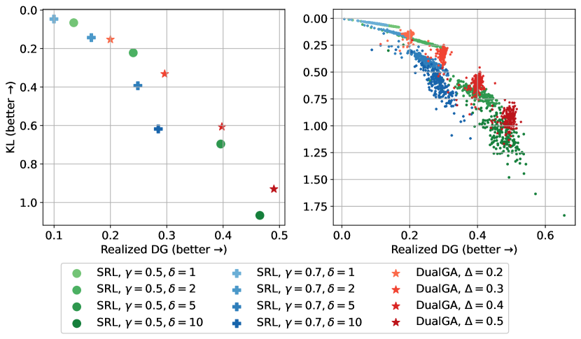
D.2.2 Pareto Optimality and Stability of DualGA
Figure 5 visualizes the detection ability (Realized DG) and distortion (KL) on the C4 dataset at the population level (left) and the individual prompt level (right), which has a similar trend as LFQA (Figure 2): Figure 5 (left) shows the Pareto optimality of the DG-KL trade-off for the DualGA, and Figure 5 (right) demonstrates DualGA’s consistency in its detection ability across different prompts. In contrast, the SRL algorithm lacks the Pareto optimality with several hyperparameters (e.g., ), and has varying levels of detection ability and distortion for different prompts.
Furthermore, Figure 6 includes a comparison with the EMS algorithm on the C4 dataset, employing -scores (defined in Appendix D.1.3) as a measure of detection ability since EMS does not divide the vocabulary into green/red lists (and thus no DG). Figure 6 uses boxplots to show the detection ability across algorithms, where the horizontal axis’s location is computed by the mean of KL divergences over 500 samples. It highlights DualGA’s stability in detection ability, as evidenced by its smaller dispersion in -scores compared to benchmark algorithms.
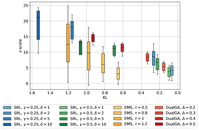
D.2.3 Robustness under Attacks
We evaluate the robustness of DualGA and other benchmark methods on three types of attacks: deletion, insertion, and substitution. The methodologies for each attack type are as follows:
-
•
Deletion: A certain percentage of tokens, referred to as the Attack Rate, is randomly selected from the watermarked text and deleted to produce the text for detection.
-
•
Insertion: We first randomly sample a position in the watermarked text and insert a randomly sampled token from the vocabulary list. This process is repeated a number of times equal to the Attack Rate multiplied by the original length of the watermarked text.
-
•
Substitution: Similar to the deletion approach, a proportion of tokens specified by the Attack Rate is randomly selected from the watermarked text. These tokens are then replaced with randomly chosen tokens from the vocabulary to create the text.
Figure 7 illustrates the detection ability of watermarking methods, measured by -values (as defined in Appendix D.1.3, lower values signify better detection), under different types and rates of attacks. Key observations include: (i) Under mild attack scenarios (Attack Rate ), most methods maintain strong performance, as reflected by their median -values below (the black dashed line in the figures). (ii) Typically, enhanced robustness appears with the increased distortion, as evidenced by higher KL values noted in the legend. (iii) Specifically for DualGA, we observe an improvement in robustness as the parameter increases. Since is the target DG and directly controls the watermarking strength, texts watermarked by DualGA with higher are easier to detect and more robust to withstand attacks.
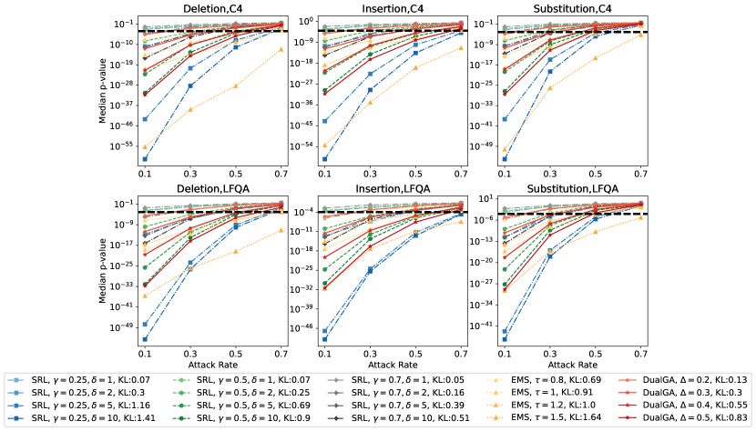
D.2.4 More Examples on Repeated Text Chunks
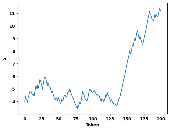
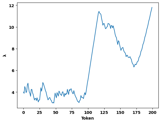

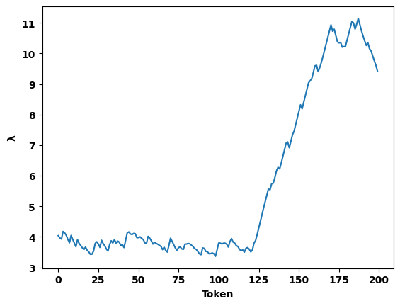

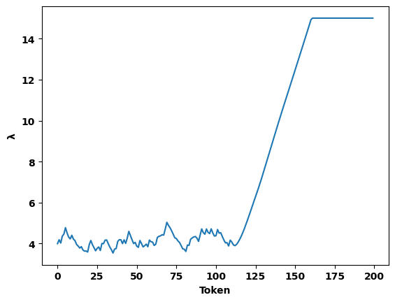
Below we give four more examples (Figure 8) of text repetition that we extract by monitoring the fluctuation curve of dual variable . The yellow blocks on the left show the generated text, while the record curves on the right depict the dynamic of with step . We select from the group of text generated from DualGA with whose ever reaches above , and in all the 4 examples that we pick out, text repetition is observed.
Appendix E Possibility for Other Variants of Watermarking
In this section, we introduce a variant for the design of watermark algorithms other than increasing the green list probability only. We hope this section serves as an inspiration for further developments of watermarking schemes. The red-green list scheme guarantees that under the null hypothesis, variables ’s are i.i.d. and mean-zero random variables. In other words, a violation of this i.i.d. assumption in any sense can serve as a watermarking scheme. Specifically, for any statistic and a corresponding watermarking paradigm such that for watermarked texts the distribution of deviates from the distribution of under the null hypothesis, we can also derive a reasonable watermarking algorithm. In both SRL (Algorithm 1) and DualGA (Algorithm 2), we construct the statistic by . Other variants of watermarking algorithms exploiting different statistics could also be developed, which may serve well in certain circumstances.
To give an example, consider using the sample autocovariance as the score statistic
which, by Theorem 7.2.1 in Brockwell and Davis (1986), has the following asymptotic property
Define . The above property says that under the null hypothesis (where ’s are i.i.d. and mean-zero), the statistic asymptotically has a standard normal distribution. In light of this, a watermarking algorithm is designed to induce the largest deviation of from a standard normal distribution, at the least cost of model distortion (measured in KL-divergence). One possible approach is to greedily minimize the stepwise autocovariance. Once we observe that is realized into the green list, we add to the red list logits of the next token and encourage the model to pick a different color; on the contrary, once we observe that is realized as red, we add to the green list logits for the next token.
For the test statistic, we define as , which satisfies the asymptotically normal property under the null hypothesis. When applying watermarks, our objective is to minimize the expectation of , which can be decomposed into stepwise minimizations of difference of the autocovariance , defined by
The new algorithm, DualGA-AutoCov is presented as Algorithm 3. The algorithm is evaluated based on its detection ability and distortion level on the C4 dataset. The comparison of DualGA-AutoCov between DualGA and other benchmarks (Figure 9 (left)) shows that DualGA-AutoCov has a similar trade-off pattern to SRL. Although the average -value of DualGA-AutoCov is larger than the original DualGA at the same distortion extent (when KL), it performs consistently better than EMS under different configurations. In the right figures of Figure 9, the robustness of DualGA-AutoCov is tested under the three common attacks given in Section 5.3. The new DualGA-AutoCov remains detectable at a significance level of when the attack rate is smaller than . This observation validates the reasonable robustness of this new formulation under mild attacks.