WaveFace: Authentic Face Restoration with Efficient Frequency Recovery

Abstract

Although diffusion models are rising as a powerful solution for blind face restoration, they are criticized for two problems: 1) slow training and inference speed, and 2) failure in preserving identity and recovering fine-grained facial details. In this work, we propose WaveFace to solve the problems in the frequency domain, where low- and high-frequency components decomposed by wavelet transformation are considered individually to maximize authenticity as well as efficiency. The diffusion model is applied to recover the low-frequency component only, which presents general information of the original image but 1/16 in size. To preserve the original identity, the generation is conditioned on the low-frequency component of low-quality images at each denoising step. Meanwhile, high-frequency components at multiple decomposition levels are handled by a unified network, which recovers complex facial details in a single step. Evaluations on four benchmark datasets show that: 1) WaveFace outperforms state-of-the-art methods in authenticity, especially in terms of identity preservation, and 2) authentic images are restored with the efficiency 10$\times$ faster than existing diffusion model-based BFR methods.

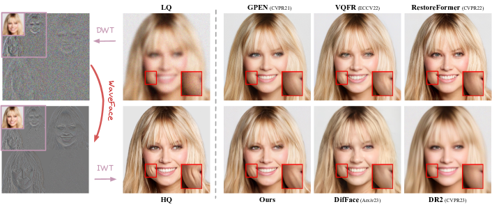
Figure 1: Left: Illustration of our frequency-aware BFR scheme. Restoration is performed in the frequency domain instead of the pixel domain. Right: Comparisons with state-of-the-art face restoration methods on degraded images. Previous methods struggle to restore facial details or the original identity while our WaveFace achieves a good balance of realness and fidelity with fewer artifacts.

1 Introduction

Blind face restoration (BFR) aims to recover high-quality (HQ) facial images from various degradations, including down-sampling, blurriness, noise, and compression artifact [1, 40, 30]. BFR is challenging since the types of degradation are generally unknown in real-world scenarios. Improvements in the restoration quality over the past few years mainly benefit from the usage of multiple facial priors. Geometric priors, including facial landmarks [3] and parsing maps [27, 2], are employed to provide explicit facial structure information. Reference priors, such as HQ images/features [43, 34, 9], are used as guidance during facial restoration. Generative priors are generally obtained by pre-trained generation models such as StyleGAN [14], which facilitate the recovery of realistic textures [2, 31, 37]. Inspired by the superior generative ability of diffusion models (DMs) [11, 28], how to unleash its potential in authentic face restoration has gained much attention.

Despite plausible restoration results being achieved, existing DMs based methods [39, 35] generally suffer from two problems: 1) DMs are trained on large images (512$\times$512), which requires massive computational resources for both training and inference, as thousands of iterations are required to obtain adequate outputs. DifFace [39], for example, takes about 25 seconds to sample an image from noise. 2) Low-quality (LQ) images are firstly diffused to an intermediate step and then denoised by an unconditional diffusion model to obtain HQ counterparts [39]. However, as shown in Fig. 1, such an unconditional generation will lead to great uncertainty in restored images, which means the original identity and facial details such as wrinkles cannot be well preserved.

To solve the above problems, we transfer the BFR task from the pixel domain to the frequency domain via Discrete Wavelet Transform (DWT). As shown in Fig. 1, an image can be decomposed and reconstructed by its four quarter-sized sub-bands: low- and high-frequency components without sacrificing information. Low-frequency sub-band mainly contains general information such as face structure while high-frequency ones contain rich facial details. By exponentially shrinking the size of input images, restoration within the frequency domain not only speeds up both training and inference but also maintains the authenticity of restoration. In the paper, we devise an efficient BFR method WaveFace that restores authentic HQ images by recovering its frequency components.

WaveFace consists of a Low-frequency Conditional Denoising (LCD) module and a High-Frequency Recovery (HFR) module. A diffusion model is used in LCD to restore the low-frequency sub-band of HQ images whose size is only 1/16 of the original image. In addition to smaller inputs, LCD leverages LQ counterparts as a condition throughout the generation to preserve the original identity. Meanwhile, HFR recovers high-frequency sub-bands decomposed at multiple DWT levels simultaneously within one step. With the frequency components restored by two modules, authentic images can be reconstructed via discrete inverse wavelet transform (IWT) within 1 ms. The contributions can be summarized as follows:

• We propose an efficient blind face restoration approach, WaveFace, that restores authentic images by recovering their frequency components individually.

• A conditional diffusion model is adopted to restore the low-frequency component, which is 1/16 the size of the original image.

• A one-pass network is used to recover high-frequency sub-bands decomposed at multiple DWT levels simultaneously.

• Comprehensive experiments demonstrate the superiority of methods in both efficiency and authenticity.

2 Related Work

2.1 Diffusion models

Diffusion Models (DMs) are emerging generative models that corrupt the data with the successive addition of Gaussian noise during the diffusion process and then learn to recover the data during denoising. State-of-the-art DMs [11] have revealed the potential in CV tasks, such as image deblurring [16, 4] and image super-resolution [26, 25].

Accelerating DMs. Despite being powerful in generation, DDPM [11] has the downside of low inference speed, which requires thousands of steps for sampling. To accelerate inference, DDIM [22] adopts a non-Markovian diffusion process that allows step skipping during sampling.

Conditional DMs. Unconditional DM-based generation leads to great uncertainty in outputs, which means they generally fail to preserve the original identity and fine-grained facial details. Therefore, conditions are injected by cross-attention layer [25], adaptive normalization layer [24], or concatenation operation [26] to control the characteristic of the synthesized images.

2.2 Blind face restoration

Facial priors exploited in blind face restoration (BFR) can be categorized into three types: geometric priors, reference priors, and generative priors.

Geometric priors based methods leverage knowledge from facial landmark [3, 6], facial parsing maps [27, 2, 42], and facial component heatmaps [38]. However, they tend to show inferior performance since degraded images fail to provide accurate and adequate structural information.

Reference priors based methods either leverage a high-quality (HQ) reference image sharing the same identity as the degraded one [18] or a pre-constructed dictionary storing HQ facial features [34, 9, 43]. Firstly, a vector-quantized (VQ) codebook is pre-trained on HQ faces via VQ-GAN [8] to provide rich facial details. Features of degraded inputs are then fused with the prior either at image [34] or latent [9, 43] level for the generation of HQ counterparts. However, reference prior is restricted by the size of the codebook, which limits the diversity and richness of generated images.

Generative priors encapsulated in pretrained face models [14, 15] are also leveraged to restore faithful faces [2, 37, 31]. PSFRGAN [2] modulates features at different scales progressively with facial parsing maps to achieve semantic-aware style transformation. GFP-GAN [31] and GPEN [37] adopt the pre-trained StyleGAN as a decoder and achieve a good balance between visual quality and fidelity of restored images. Recently, diffusion models [11, 28] have shown the powerful generative ability in restoring HQ content from noisy images. Inspired by the ability, DifFace [39] firstly maps low-quality (LQ) inputs into an intermediate step of the denoising process, from which its HQ counterpart is recursively sampled. DR2 [35] employs the diffusion model to remove degradations, followed by a super-resolution model to obtain HQ counterparts.

Nevertheless, previous DM-based BFR methods are performed in the pixel domain, where large inputs require massive computational resources for both training and inference. Besides, they both apply the unconditional scheme that leads to significant uncertainty in restored results.

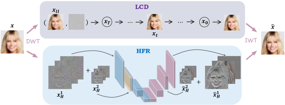
Figure 2: Overall framework of WaveFace. It consists of a Low-frequency Conditional Denoising (LCD) module and a High-Frequency Refinement (HFR) module. LCD (Sec. 4.1) predicts clean samples $\bm{x}_{0}$ from noise conditioned on LQ inputs through $T$ steps. Meanwhile, high-frequency sub-bands are concatenated as HFR (Sec. 4.2) inputs to recover vivid facial details. The predicted frequency components are projected back to the image via IWT.

3 Preliminary

Discrete Wavelet Transformation (DWT). DWT decomposes an image into low-frequency and high-frequency sub-bands. The low-frequency component presents general information while high-frequency ones express facial details in the vertical, horizontal, and diagonal directions. In the paper, we use Haar wavelet for DWT, which is widely used in real-world applications due to simplicity [23].

Given an image $\bm{x}\in\mathbb{R}^{H\times W\times 3}$, its low-frequency sub-band $\bm{x}_{ll}^{1}\in\mathbb{R}^{H/2\times W/2\times 3}$ and high-frequency sub-bands $\bm{x}_{lh}^{1},\bm{x}_{hl}^{1}$, and $\bm{x}_{hh}^{1}\in\mathbb{R}^{H/2\times W/2\times 3}$ can be decomposed by:

$$\bm{x}_{ll}^{1},\bm{x}_{lh}^{1},\bm{x}_{hl}^{1},\bm{x}_{hh}^{1}=DWT(\bm{x}),$$ (1)

where $DWT(\cdot)$ refers to the DWT operation. Despite that the input size is decreased by a factor of four ($H/2\times W/2$) after a single DWT decomposition, DWT can be performed on the low-frequency component to further reduce the computational cost and expedite the inference:

$$\bm{x}_{ll}^{J+1},\bm{x}_{lh}^{J+1},\bm{x}_{hl}^{J+1},\bm{x}_{hh}^{J+1}=DWT(\bm{x}_{ll}^{J}),$$ (2)

where $J$ is level of DWT decomposition and $\bm{x}_{ll}^{J+1},\bm{x}_{lh}^{J+1},\bm{x}_{hl}^{J+1},\bm{x}_{hh}^{J+1}\in\mathbb{R}^{{H}/{2^{(J+1)}}\times W/2^{(J+1)}\times 3}$. Reversibly, given the frequency sub-bands, an image can be reconstructed via discrete inverse wavelet transform (IWT):

$$\bm{x}=IWT(\bm{x}_{ll}^{1},\bm{x}_{lh}^{1},\bm{x}_{hl}^{1},\bm{x}_{hh}^{1}).$$ (3)

Diffusion Models. Training of diffusion models (DMs) consists of a diffusion process and a denoising process. Diffusion process transforms an image from the real data distribution $\bm{y}_{0}\sim q(\bm{y}_{0})$ into a pure Gaussian noise $\bm{y}_{T}$ by successively applying the following Markov diffusion kernel:

$$q(\bm{y}_{t}|\bm{y_{t-1}})=\mathcal{N}(\bm{y}_{t};\sqrt{1-\beta_{t}}\bm{y}_{t-1},\beta_{t}\bm{I}),$$ (4)

where $\{\beta_{t}\}_{t=1}^{T}$ is a pre-defined or learned noise variance schedule. The marginal distribution at arbitrary timestep $t$ can be denoted as:

$$q(\bm{y}_{t}|\bm{y}_{0})=\mathcal{N}(\bm{y}_{t};\sqrt{\alpha_{t}}\bm{y}_{0},(1-\alpha_{t})\bm{I}),$$ (5)

where $\alpha_{t}=\prod_{s=1}^{t}(1-\beta_{s})$. Given $\bm{y}_{t}$, the denoising process aims to recover $\bm{y}_{0}$ by recursively learning the transition from $\bm{y}_{t-1}$ to $\bm{y}_{t}$, which is defined as the following Gaussian distribution:

$$p_{\theta}(\bm{y}_{t-1}|\bm{y}_{t})=\mathcal{N}\left(\bm{y}_{t-1};\bm{\mu}_{\theta}(\bm{y}_{t},t),\bm{\Sigma}_{\theta}(\bm{y}_{t},t)\right),$$ (6)

where parameters $\theta$ are optimized by a denoising network $\bm{\epsilon}_{\theta}$ that predicts $\bm{\mu}_{\theta}(\bm{y}_{t},t)$ and $\mathbf{\Sigma}_{\theta}(\bm{y}_{t},t)$.

4 Methodology

In the paper, WaveFace is proposed to handle blind face restoration (BFR) in the frequency domain. The framework is depicted in Fig. 2. First, degraded images are mapped to the frequency domain via Discrete Wavelet Transformation (DWT) (Sec. 3). The proposed Low-frequency Conditional Denoising (LCD) module (Sec. 4.1) and High-Frequency Recovery (HFR) module (Sec. 4.2) are adopted on the low- and high-frequency components respectively to remove degradations and restore facial details. Recovered frequency components are used for the image reconstruction.

4.1 Low-frequency Conditional Denoising

As shown in Fig. 1, the low-frequency component is similar to the down-sampled version of the original image, which largely determines the restoration quality. Due to its powerful generative ability from noisy inputs, a diffusion model (DM) is adopted in LCD to restore the low-frequency sub-band of high-quality (HQ) images.

Conditional DM. We denote the low-frequency sub-band of a pair of LQ and HQ images as ($\bm{x}^{j}_{ll_{0}}$, $\bm{y}^{j}_{ll_{0}}$). Since the low-frequency sub-band only contains a single map after DWT, the DWT levels $j$ and $ll$ are omitted in this section for simplicity. According to the diffusion process defined in Eq. 5, images are successively destroyed by Gaussian noise as timestep $t$ increases, which means the distribution $q(\bm{x}_{T}|\bm{x}_{0})\approx q(\bm{y}_{T}|\bm{y}_{0})\approx\mathcal{N}(0,\bm{I})$ after a large timestep $T$. Given this assumption, our LCD aims to learn the posterior distribution $p(\bm{y}_{0}|\bm{x}_{0})$:

$$p(\bm{y}_{0}|\bm{x}_{0})=\int q(\bm{y}_{T}|\bm{x}_{0})\prod_{t=1}^{T}p_{\theta}(\bm{y}_{t-1}|\bm{y}_{t})\mathrm{d}\bm{y}_{1:T},$$ (7)

where $p_{\theta}(\bm{y}_{t-1}|\bm{y}_{t})$ refers to the unconditional denoising process defined in Eq. 6. However, the unconditional scheme fails to preserve the original identity due to the lack of guidance during generation. To solve the problem, the low-frequency sub-band of LQ images $\bm{x}_{0}$ are injected as the condition for the denoising process:

$$p_{\theta}(\bm{y}_{t-1}|\bm{y}_{t},\bm{x}_{0})=\mathcal{N}\left(\bm{y}_{t-1};\bm{\mu}_{\theta}(\bm{y}_{t},t,\bm{x}_{0}),\bm{\Sigma}_{\theta}(\bm{y}_{t},t,\bm{x}_{0})\right),$$ (8)

where $\bm{x}_{0}$ is injected by concatenating with the input $y_{t}$ along the channel dimension.

Objectives. Following DDPM [11], the denoising network $\bm{\epsilon}_{\theta}$ is trained to predict noise vectors with the objective:

$$L_{LCD}=\mathbb{E}_{\bm{y}_{0},t,\bm{\epsilon}_{t}\sim\operatorname{\mathcal{N}}(\mathbf{0},\operatorname{\mathbf{I}})}\Big{[}||\bm{\epsilon}_{t}-\bm{\epsilon}_{\theta}(\bm{y}_{t},\bm{x}_{0},t)||^{2}\Big{]}.$$ (9)

During inference, with the learned parameterized Gaussian transitions $p_{\theta}(\bm{y}_{t-1}|\bm{y}_{t},\bm{x}_{0})$, the low-frequency sub-band of HQ images can be recovered from a random Gaussian noise $\bm{y}_{T}\sim\operatorname{\mathcal{N}}(\mathbf{0},\operatorname{\mathbf{I}})$ by recursively applying:

$$\bm{y}_{t-1}=\frac{1}{\sqrt{\alpha_{t}}}\left(\bm{y}_{t}-\frac{\beta_{t}}{\sqrt{1-\bar{\alpha}_{t}}}\bm{\epsilon}_{\theta}(\bm{y}_{t},\bm{x}_{0},t)\right)+\sigma_{t}\bm{z},$$ (10)

where $\bm{z}\sim\mathcal{N}(\mathbf{0},\operatorname{\mathbf{I}})$, $\alpha_{t}=1-\beta_{t}$, and $\bar{\alpha}_{t}=\prod_{i=1}^{t}\alpha_{i}$.

(a) $J=3\quad(\times 64)$

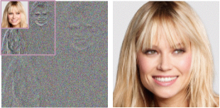
(b) $J=2\quad(\times 128)$

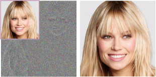
(c) $J=1\quad(\times 256)$

Figure 3: Visualization of DWT frequency components and images reconstructed by the low-frequency sub-band of an HQ image and high-frequency sub-bands of its LQ counterpart. DWT level $J$ and resolution of low- / high-frequency sub-bands ($\times N$) are reported.

Trade-off between efficiency and quality. Training a DM on large inputs ($\times$512 or more) requires massive computational resources and the evaluation takes thousands of steps to sample from the noise. Although this problem can be alleviated by adopting low-frequency sub-bands at higher DWT levels, multiple times of decomposition will also lead to information reduction. How to set DWT level wisely is the key to balance between efficiency and authenticity.

To illustrate how DWT level $J$ affects the authenticity, we visualize the image reconstructed by the low-frequency component of HQ images and the corresponding high-frequency ones of its LQ counterpart at different DWT levels in Fig. 3. Although noisy at the high-frequency part, the quality of images reconstructed at $J\leq 2$ is acceptable, with key facial features such as wrinkles still preserved. However, the mosaic effect starts to emerge when $J$ keeps increasing. Ablation studies about the effect of DWT level on training/inference are shown in Sec. 5.2.1. In the paper, $J$ is set as 2 empirically.

4.2 High-frequency Recovery

Although the general face information is restored by LCD, rich facial details are generally embedded in the high-frequency component, as shown in Fig. 1, which improves the authenticity of restored images. High-frequency sub-bands at multiple DWT levels also vary in size, which means more than one diffusion model is required for the recovery. To avoid the extravagant computational cost, we adopt a U-shaped network that can recover high-frequency sub-bands at multiple DWT levels at the same time and takes only one step for inference.

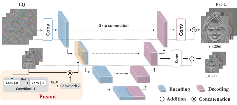
Figure 4: Illustration of high-frequency recovery (HFR) module.

Given a LQ and HQ image pair $(\bm{x},\bm{y})$ and their high-frequency sub-bands: $\bm{x}^{j}_{H}=\{\bm{x}^{j}_{lh},\bm{x}^{j}_{hl},\bm{x}^{j}_{hh}\}$ and $\bm{y}^{j}_{H}=\{\bm{y}^{j}_{lh},\bm{y}^{j}_{hl},\bm{y}^{j}_{hh}\}$, where $j\in\{1,2\}$ refers to DWT level, the framework our high-frequency recovery (HFR) module is illustrated in Fig. 4. HFR takes high-frequency sub-bands of LQ images that are channel-wise concatenated as inputs and outputs the recovered ones $\bm{\hat{x}}^{j}_{H}$ as follows:

$$\bm{F}^{1}_{H},\bm{F}^{2}_{H}=\mathcal{U}_{\phi_{u}}(\mathcal{H}_{\phi_{in}}(\bm{x}^{1}_{H}),\mathcal{F}_{\phi_{f}}(\bm{x}^{2}_{H})),$$ (11)

$$\bm{\hat{x}}^{j}_{H}=\mathcal{H}_{\phi^{j}_{out}}(\bm{F}^{j}_{H})+\bm{x}^{j}_{H},\quad j\in\{1,2\},$$ (12)

where $\mathcal{U}(\cdot)$, $\mathcal{H(\cdot)}$, $\mathcal{F}(\cdot)$ denotes the U-shaped network, the convolutional layer, and the fusion module with the parameter $\phi_{u}$, $\phi^{j}_{in/out}$, and $\phi_{f}$, respectively. $\bm{F}^{1}_{H}$, $\bm{F}^{2}_{H}$ represents feature maps of the last and penultimate decoding layers of the U-shaped network. Considering efficiency, the fusion module only contains two stacked ConvBlocks that apply 3$\times$3 and 1$\times$1 convolutional layers with ReLU in between, followed by concatenation with the input.

Objectives. We adopt two loss terms for the training of HFR: recovery loss $\mathcal{L}_{r}$ and content loss [33] $\mathcal{L}_{c}$. The recovery loss is applied not only to restore HQ high-frequency sub-bands $\bm{y}^{j}_{H}$ at each level but also to the image $\bm{y}^{j-1}$ reconstructed via inverse wavelet transform (IWT):

$$\mathcal{L}_{r}=\sum_{j}(||\bm{\hat{x}}^{j}_{H}-\bm{y}^{j}_{H}||+\alpha||IWT(\bm{y}^{j}_{ll},\bm{\hat{x}}^{j}_{H})-\bm{y}^{j-1}||),$$ (13)

where $IWT(\cdot)$ denotes IWT operation and $\alpha=1$ is the parameter balancing losses between the frequency domain and the pixel domain. In addition to minimizing the pixel-wise distance, the content loss is applied to maximize the luminance, contrast, and structural similarity of the restored and original HQ image:

$$\mathcal{L}_{c}=1-SSIM(IWT(\bm{y}^{2}_{ll},\bm{\hat{x}}^{2}_{H},\bm{\hat{x}}^{1}_{H}),\bm{y}).$$ (14)

The overall objective of HFR is $\mathcal{L}_{HFR}=\mathcal{L}_{r}+\lambda\mathcal{L}_{c}$, where the weighting parameter $\lambda$ is set as 10.

5 Experiments

5.1 Settings and Datasets

Training Dataset. FFHQ [14] is used as the training set, which contains 70,000 high-quality (HQ) face images. Following BFR benchmark works [34, 9], we resize HQ images to the resolution of $512\times 512$, and then synthesize low-quality (LQ) counterparts as follows:

$$\bm{x}=\left\{\left[\left(\bm{y}\otimes\bm{k}_{\sigma}\right){\downarrow_{s}}+\bm{n}_{\delta}\right]_{\text{JPEG}_{q}}\right\}{\uparrow_{s}},$$ (15)

where a HQ image $\bm{y}$ is firstly blurred by a Gaussian kernel $\bm{k}_{\sigma}$, followed by a downsampling of scale $s$. Afterward, Gaussian noise $\bm{n}_{\delta}$ and JPEG compression with quality factor $q$ are applied to the image, which is then upsampled back to the original size to obtain its LQ counterpart $\bm{x}$. The hyper-parameters $\sigma$, $s$, $\delta$, and $q$ are uniformly sampled from $[0.1,15]$, $[0.8,32]$, $[0,20]$, and $[30,95]$ respectively.

Testing Dataset. We evaluate WaveFace on a synthetic dataset: CelebA-Test and three real-world datasets: LFW-Test [12], WebPhoto-Test [31], and WIDER-Test [43]. CelebA-Test contains 3000 HQ images from CelebA-HQ [13], and LQ counterparts are synthesized via Eq. (15) with the same degradation setting. In terms of three real-world datasets, LFW-Test contains 1711 mildly degraded face images in the wild, which comprises the first image for each person in LFW [12]. WebPhoto-Test includes 407 images crawled from the internet, some of which are old photos with severe degradation. WIDER-Test consists of 970 images with severe degradations from the WIDER dataset [36].

Evaluation Metrics. For evaluation, we adopt two pixel-wise metrics (PSNR and SSIM), a reference perceptual metric (LPIPS [41]), and a non-reference perceptual metric (FID [10]). To measure the consistency of identity, the angle between embeddings extracted by ArcFace (“Deg.”) [5] is used. All metrics are used for the evaluation of synthetic data while only FID is used for real-world datasets due to the lack of referential HQ images.

Implementation Details. The DWT decomposition level is set as 2, which reduces the input size of the diffusion model from 512$\times$512 to 128$\times$128. We train LCD and HFR individually with Adam [17] optimizer. LCD is trained for 200K iterations with the learning rate $1e\text{-}4$ and batch size 32. For HFR, the training takes 70K iterations. The learning rate gradually decays from $1e\text{-}3$ to $1e\text{-}5$ by a factor of 0.1.

5.2 Ablation Studies

5.2.1 Low-frequency Conditional Denoising

DWT Levels. We conduct an experiment to investigate how the level of wavelet decomposition (DWT) affects the efficiency and authenticity. DWT is applied 0, 1, 2, 3 times on the training set, where the resolution of the diffusion model (DM)’s input becomes 512$\times$512, 256$\times$256, 128$\times$128, and 64$\times$64, respectively. The number of parameters and the inference time are used to evaluate the efficiency while PSNR and SSIM are used to evaluate authenticity. The comparison results are reported in Tab. 1.

Table 1: Comparison between state-of-the-art diffusion model-based BFR methods and ours at different DWT levels in terms of efficiency and authenticity. The best and the second best performances are highlighted and underlined.

Method	Level	Resolution	#Param. (M)	Time (s)	PSNR$\uparrow$	SSIM$\uparrow$
DifFace [39]	-	$\times$ 512	175.38	25.04	19.06	0.46
DR2 [35]	-	$\times$ 256	93.56	8.76	22.89	0.57
WaveFace	0	$\times$ 512	109.06	19.37	26.42	0.65
	1	$\times$ 256	71.41	8.12	27.08	0.73
	2	$\times$ 128	25.36	1.97	26.97	0.71
	3	$\times$ 64	3.9	1.46	24.81	0.46

In comparison with the model trained on original images ($\times$512), our frequency-aware scheme applies DM on the low-frequency sub-band only, which avoids some unknown noise on high-frequency components. Thus, the restoration quality improves after the wavelet decomposition is applied once. The quality can be maintained until the DWT level increases to 2, where the inference process is accelerated by $10\times$. However, the performance is significantly harmed when the DWT level further increases (3 or higher) as too many details in the low-frequency component have been reduced. DWT level is set as 2 throughout the experiments to achieve the trade-off between the efficiency and the quality of restoration.

We also compare the efficiency with two DM-based BFR methods: DifFace [39] and DR2 [35]. To make a fair comparison, the inference time refers to the time of the whole denoising process, which starts from the pure Gaussian noise. The quality of generated images cannot compared with that reported in Tab. 3 as images are generated with pre-/post-processing and fewer sampling steps in their methods. As can be seen, our method achieves better restoration quality at a lower computational cost.

Conditions. To investigate how the condition facilitates the restoration, we first remove the condition from the input of our LCD module and train an unconditional diffusion model for 200K iterations for a fair comparison. The restored face is denoted by “Uncond.” in Fig. 5. We notice that not only the identity is not preserved but also the image quality drops significantly. This could be attributed to the slow convergence of the unconditional training manner [24].

Additionally, we compare with two widely-used conditioning schemes: adaptive group normalization layers (AdaGN) [24] and cross-attention [25]. We replace the low-frequency sub-band of LQ images with the corresponding identity embedding extracted by Arcface [5], which are subsequently injected via AdaGN. Furthermore, a cross-attention layer is added to condition the denoised image at each step with the LQ low-frequency information. Experimental details of the two schemes will be discussed in supplementary materials. The restored images are shown in Fig. 5 as “AdaGN” and “Cross-Att.”, respectively. Although the original identity is preserved by the AdaGN scheme, the background is not well restored. A possible reason is that the identity-related condition is performed at the latent level only, which fails to provide pixel-wise constraints. On the other hand, despite the cross-attention scheme achieves a comparable restoration result with ours (“Concat.”), the extra layer requires more computational resources.

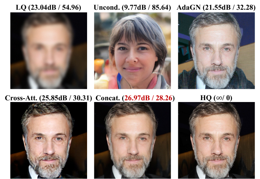
Figure 5: Qualitative comparison of different conditioning schemes on CelebA-Test. We adopt “Concat.” in WaveFace. PSNR($\uparrow$) / Deg.($\downarrow$) are reported.

Table 2: Ablation studies of the effectiveness of our high-frequency recovery (HFR) module. $\bm{x}_{H}$ denotes high-frequency sub-bands of LQ images and $1,2$ stands for the level of wavelet decomposition. Best performance is indicated by Red.

	PSNR$\uparrow$	SSIM$\uparrow$	LPIPS$\downarrow$	FID$\downarrow$
LCD + $\bm{x}^{1}_{H}$ + $\bm{x}^{2}_{H}$	24.353	0.430	0.537	17.264
LCD + HFR1 + $\bm{x}^{2}_{H}$	26.081	0.609	0.481	14.020
LCD + $\bm{x}^{1}_{H}$ + HFR2	24.819	0.460	0.536	15.293
LCD + HFR1 + HFR2 (Ours)	26.967	0.711	0.343	13.062

5.2.2 High-frequency Recovery

To investigate the effectiveness of our High-frequency Recovery (HFR) module, we replace the recovered high-frequency sub-bands at different DWT levels with that of low-quality (LQ) images for image reconstruction. Quantitative comparisons on the restoration quality of different schemes are reported in Tab. 2. The restoration quality drops significantly when HFR is removed with a decline of $2.62$ dB in PSNR. Besides, the lack of recovered high-frequency components at different DWT levels deteriorates the restoration quality to varying extents. In comparison with those at level 2 ($\times$128), high-frequency sub-bands at level 1 ($\times$256) contribute more to the restoration quality.

The exemplar illustrated in Fig. 6 helps to understand intuitively. Before our HFR is applied (Row 2), the restored image contains cluttered noise and lacks details such as hairstyle due to messy high-frequency sub-bands of LQ images. The quality improves when the image is constructed with the refined high-frequency component (Row 3), which is less noisy and presents fine-grained details.

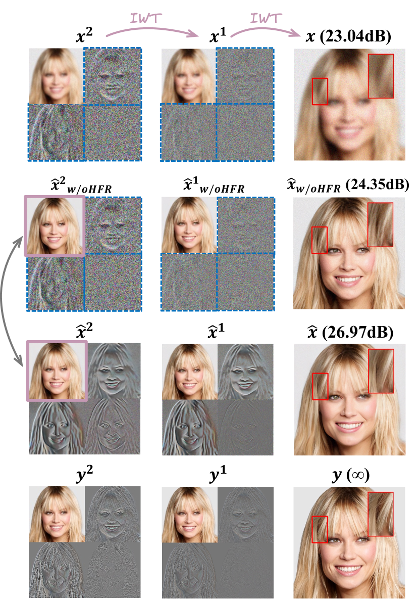
Figure 6: Qualitative comparison between images reconstructed at different DWT levels with and without (w/o) HFR module on CelebA-Test. $\bm{x}$, $\bm{\hat{x}}$ and $\bm{y}$ denotes LQ images, restored images, and HQ images. $\bm{x^{j}}(j\in\{1,2\})$ denotes frequency components at $j$-th DWT level. PSNR($\uparrow$) of the restored images are reported.

Table 3: Quantitative comparison on CelebA-Test for blind face restoration. “Deg.” refers to the angle between identity embeddings of restored images and HQ counterparts. The best and the second best performances are highlighed and underlined.

.5pt=0.1cm Methods PSNR$\uparrow$ SSIM$\uparrow$ LPIPS$\downarrow$ FID$\downarrow$ Deg.$\downarrow$ Input 23.038 0.389 0.586 67.505 54.958 GPEN [37] 24.319 0.603 0.440 22.251 38.473 GFP-GAN [31] 24.771 0.674 0.361 14.501 36.958 VQFR [9] 23.735 0.614 0.358 14.048 38.684 RestoreFormer [34] 24.191 0.636 0.364 12.000 34.752 CodeFormer [43] 25.071 0.672 0.359 14.385 37.677 DR2 [35] 23.583 0.613 0.402 14.671 51.030 DifFace [39] 24.155 0.667 0.390 13.379 49.958 WaveFace 26.967$\uparrow$1.90 0.711 0.343 13.062 28.263$\uparrow$6.49

(a) LQ

(b) GPEN [37]

(c) GFPGAN [31]

(d) VQFR[9]

(e) RestoreFormer [34]

(f) DifFace [39]

(g) DR2 [35]

(h) Ours

(i) HQ

Figure 7: Qualitative comparison with state-of-the-art BFR methods on CelebA-Test. Our method achieves a better restoration quality with the original identity and facial details well preserved. (Zoom in for best view).

5.3 Comparisons with State-of-the-Art Methods

State-of-the-art (SOTA) methods used for comparison include generative prior based methods (GPEN [37] and GFPGAN [31]), reference prior based methods (VQFR [9] and RestoreFormer [34]) and recent diffusion model-based methods (DifFace [39] and DR2 [35]). Evaluations are conducted on both synthetic and real-world datasets.

Synthetic dataset. Quantitative comparison on CelebA-Test [13] are illustrated in Tab. 3. WaveFace achieves the best scores on reference-based metrics and ranks second on FID. Apart from the better restoration quality, our method faithfully preserves the identity with the minimum angle between identity embeddings and their HQ counterparts, outperforming the second-best method by 6.5 degrees.

Additionally, we present the qualitative comparison with SOTA methods on images with increasing degradations in Fig. 7. GFPN and GFPGAN generally produce over-smoothed results. VQFR and RestoreFormer introduce obvious artifacts especially when the inputs are corrupted by mild or severe degradation. Besides, the above methods fail to preserve the identity since they are highly dependent on the StyleGAN prior, where the pre-defined latent space limits the diversity in restored results. Diffusion prior-based methods (DifFace and DR2) tend to generate faithful images with minor artifacts. However, due to the lack of condition during generation, both methods still suffer from the failure in identity preservation. On the contrary, our method, with the help of diffusion prior as well as the injected condition, is capable of generating high-quality facial images with fewer artifacts and, meanwhile, is faithful to the original identity.

(a) LQ

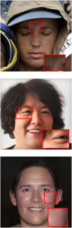
(b) GPEN [37]

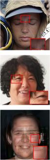
(c) GFPGAN [31]

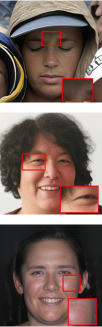
(d) VQFR[9]

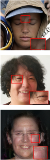
(e) RestoreFormer [34]

(f) SwinIR [19]

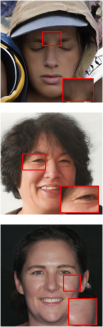
(g) DifFace [39]

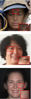
(h) DR2 [35]

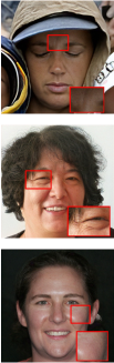
(i) Ours

Figure 8: Qualitative comparison with state-of-the-art BFR methods on real-world datasets, including LFW-Test (first row), WebPhoto-Test (second row), and WIDER-Test (third row). (Zoom in for best view).

Table 4: Quantitative comparisons on three real-world datasets (-Test) in terms of FID. The best and the second best performances are highlighted and underlined.

Methods	LFW	WebPhoto	WIDER
Input	124.974	170.112	199.961
GPEN [37]	50.792	80.572	46.340
GFP-GAN [31]	49.560	87.584	39.499
VQFR [9]	50.867	75.348	44.107
RestoreFormer [34]	47.750	77.330	49.817
CodeFormer [43]	51.863	83.193	38.784
DR2 [35]	45.298	112.344	45.348
DifFace [39]	45.227	87.811	37.112
WaveFace	43.175	81.525	36.913

Real-world datasets. We compare with SOTA methods on three real-world datasets in terms of FID score, which measures the KL divergence between the distribution of restored images and that of HQ images in FFHQ [14]. To reduce the large gap between the synthetic degradations and real-world ones, following previous diffusion prior-based methods [39, 19], a pre-denoising network [19] is applied before our method to handle the unknown degradations. Quantitative results with SOTA methods are reported in Tab. 4. WaveFace outperforms state-of-the-art (SOTA) methods on LFW-Test [12] and WIDER-Test [43] and beats previous diffusion model based BFR methods on WebPhoto-Test [31]. As mentioned in DifFace [39], the FID score may not be the most suitable evaluation metric for WebPhoto-Test, as a total of 407 images is significantly distant from representing the data distribution.

Three typical examples are shown in Fig. 8 with the increasing degradation level. It is observed that previous BFR methods tend to generate either hazy or unnatural faces. Some methods even fail to generate adequate restored results when handling severe degradations (Row 3). In contrast, our approach provides much more natural and realistic results with rich details such as wrinkles.

6 Conclusion

We propose WaveFace to solve the task in the frequency domain to achieve the trade-off between efficiency and authenticity. Efficiency is achieved by applying a diffusion model only on the low-frequency sub-band whose size is 1/16 of the original image. Meanwhile, high-frequency components decomposed at multiple DWT levels are recovered simultaneously by a one-forward framework, which ensures the preservation of facial details.

Limitations. There is a considerable gap between real-world degradations and the simulated ones (Eq. 15), leading to inferior results in some cases. Our future work will focus on how to simulate degradations that fit real-world scenarios.

Supplementary Material

A Experimental Details

A.1 Conditioning scheme

In Sec. 5.2, we discuss the effectiveness of several widely-used conditioning schemes. In this section, we will provide more details about “AdaGN” and “Cross-Att.”.

AdaGN. Adaptive group normalization (AdaGN) conditions the denoising network at the latent level, where the timestep and latent vector are incorporated into each residual block after group normalization:

$$\text{AdaGN}(\bm{h},t,\bm{z}_{ll})=\bm{z}_{s}(t_{s}\text{GroupNorm}(h)+t_{b}),$$ (16)

where $\bm{z}_{s}\in\mathbb{R}^{d}=\text{Affine}(\bm{z}_{ll})$ refers to identity features of LQ images $\bm{x}_{0}$ extracted by ArcFace [5] after the affine transformation. $(t_{s},t_{b})\in\mathbb{R}^{2\times d}=MLP(\psi(t))$ is the output of a Multi-Layer Perceptron (MLP) with a sinusoidal encoding function $\psi$. $d$ denotes the dimension of embeddings.

Cross-Att. Cross-attention (CA) layer can improve the model performance via the inner relationship between inputs from multiple modalities [7, 25]. In the paper, cross-attention is adopted to complement the denoised HQ sample at each timestep $\bm{y}_{t}$ with its LQ counterpart $\bm{x}_{0}$:

$$\text{CA}(Q,K,V)=\text{softmax}\left(\frac{QK^{T}}{\sqrt{d}}\right)\cdot V,$$ (17)

$$Q=W_{Q}\cdot\bm{x}_{0},\quad K=W_{K}\cdot\bm{y}_{t},\quad V=W_{V}\cdot\bm{y}_{t},$$ (18)

where $W_{Q},W_{K},W_{V}$ are learnable projection matrices [29]. $\text{CA}(\cdot)$ refers to the cross-attention operation, which is the pixel-wise dot product between HQ feature maps $V$ and corresponding attention scores.

B Additional Experimental Results

Methods	CelebA	LFW	WebPhoto	WIDER
Input	14.114	8.575	12.664	13.498
GPEN [37]	7.760	3.853	4.498	4.105
GFP-GAN [31]	4.171	3.954	4.248	3.880
VQFR [9]	3.775	3.574	3.606	3.054
RestoreFormer [34]	4.436	4.145	4.459	3.894
CodeFormer [43]	4.680	4.520	4.708	4.165
DR2 [35]	4.998	4.736	6.159	5.171
DifFace [39]	4.500	4.220	4.666	4.688
DM	4.898	4.784	4.860	4.988
WaveFace	4.421	4.133	4.383	4.963
GT	4.373	-	-	-

Table B.1: Quantitative comparisons on synthetic and real-world datasets (-Test) in terms of NIQE$\downarrow$.

B.1 Discussion on Non-Reference Metric

In Tab. 4, we report the performance of state-of-the-art (SOTA) methods on synthetic and real-world datasets in terms of FID score. In this section, we further consider two commonly used non-reference metrics: NIQE [21] and NRQM [20]. The results are reported in Tab. B.1 and Tab. B.2, respectively. As can be seen, despite the superiority of our method in terms of identity preserving and facial detail recovery, it shows inferior performance on these non-reference metrics. We also notice that images restored by some methods even unreasonably beat ground truth (GT) on CelebA-Test.

Methods	CelebA	LFW	WebPhoto	WIDER
Input	6.042	2.810	2.044	1.358
GPEN [37]	8.514	8.482	7.584	8.112
GFP-GAN [31]	7.985	7.782	7.750	7.990
VQFR [9]	8.657	8.564	8.457	8.792
RestoreFormer [34]	8.495	8.572	8.133	8.537
CodeFormer [43]	8.339	8.217	7.457	8.370
DR2 [35]	6.906	6.049	4.423	5.219
DifFace [39]	7.724	6.322	4.929	4.728
DM	7.121	7.125	7.091	7.167
WaveFace	7.732	7.753	6.749	6.541
GT	7.909	-	-	-

Table B.2: Quantitative comparisons on synthetic and real-world datasets (-Test) in terms of NRQM$\uparrow$.

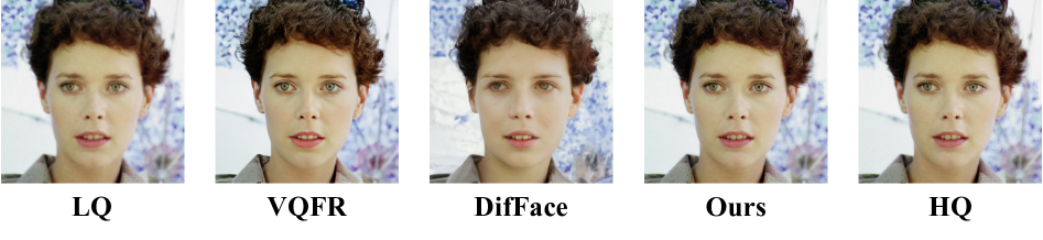
Figure B.1: Qualitative comparison between generative prior-based and diffusion model-based methods.

Figure B.2: Samples generated by benchmark diffusion model.

To explore the reason behind this, the qualitative comparison is conducted between a generative prior-based method (VQFR [9]) and diffusion model-based methods (DifFace [39] and ours). As shown in Fig. B.1, although the image generated by VQFR provides better sharpness, it contains many artifacts. For example, the hair and eyelashes present an unnatural woolen texture, which deteriorates the image’s authenticity. On the contrary, diffusion model-based methods can yield more photorealistic faces with human-like textures.

To further investigate the performance of diffusion models on these two metrics, we randomly sample the same number of images as the corresponding dataset with a benchmark pre-trained diffusion model and evaluate the quality by NIQE and NRQM. Some generated images are depicted in Fig. B.2 and quantitative results are denoted as “DM” in Tab. B.1 and Tab. B.2. As shown in both tables, even images generated by the benchmark diffusion model underperform those by GAN-based methods on these non-reference metrics, which challenges the common finding that diffusion models beat GANs in image synthesis [7, 25, 23].

Both qualitative and quantitative results illustrate that these two non-reference metrics cannot well represent the performance of BFR methods. More investigations are called to study the appropriate evaluation metrics for BFR.

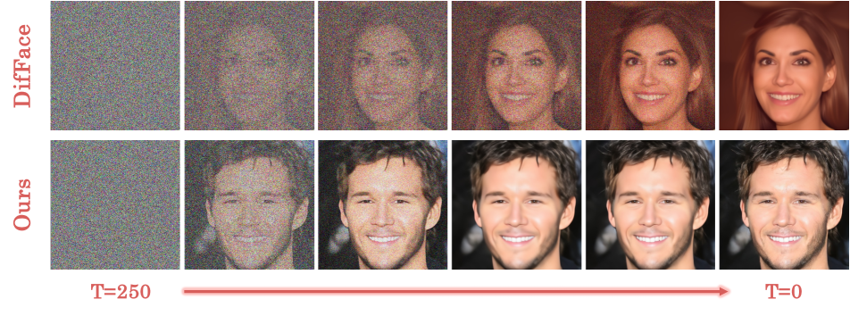
Figure B.3: Visualization of denoising process of the unconditional diffusion model adopted in DifFace [39] and our conditional one.

B.2 Degradation types

Apart from the classical degradation model (Eq. 15), we adopt the second-order degradation process proposed by RealESRGAN [32], where classical degradations are applied repeatedly to mimic real-world degradation. Following the settings in Sec. 5.1, we train both LCD and HFR modules on FFHQ [14] with RealESRGAN degradations. To evaluate the model, a corresponding evaluation set is synthesized based on 3000 CelebA-HQ images, namely CelebA-Test-RESR.

The performances of SOTA methods and our method on CelebA-Test-RESR and real-world datasets are reported in Tab. B.3 and Tab. B.4, respectively. As can be seen, the model trained on data with RealESRGAN degradations outperforms that on classical degradations, which demonstrates that RealESRGAN degradations can better imitate real-world degradations. The qualitative comparison between SOTA methods and ours is illustrated in Fig. B.4. Our method (WaveFace) is able to deliver authentic results with both identity information and fine-grained details well preserved. For example, our method restores more details of the earrings in 2nd column.

Table B.3: Quantitative comparison on CelebA-Test-RESR for blind face restoration. “Deg.” refers to the angle between identity embeddings of restored images and HQ counterparts. Best performances are highlighed.

.5pt=0.1cm Methods PSNR$\uparrow$ SSIM$\uparrow$ LPIPS$\downarrow$ FID$\downarrow$ Deg.$\downarrow$ Input 18.886 0.449 0.574 48.968 39.910 VQFR [9] 18.167 0.516 0.459 11.911 35.104 DifFace [39] 18.321 0.540 0.489 12.353 43.773 WaveFace 19.126 0.576 0.436 11.336 32.863

Table B.4: Quantitative comparisons on three real-world datasets (-Test) in terms of FID_↓. Best performances are highlighed.

Methods	LFW	WebPhoto	WIDER
Input	124.974	170.112	199.961
WaveFace (Classical)	43.175	81.525	36.913
WaveFace (RealESRGAN)	46.711	78.438	35.750

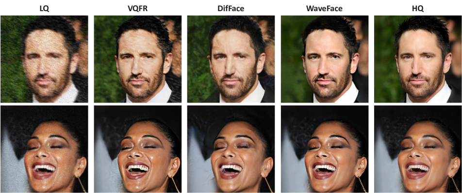
Figure B.4: Qualitative comparison on CelebA-Test-RESR.

B.3 Denoising Process Visualization

We illustrate the denoising process of the diffusion model used in our low-frequency conditional denoising (LCD) module and the unconditional one adopted in DifFace [39] in Fig. B.3. Both models are trained on FFHQ [14] and tested on CelebA-Test [13]. We take DDIM [28] as the sampling scheme, which takes 250 steps to sample an image from a pure Gaussian noise. It can be easily observed that conditional DM (Ours) achieves a faster sampling convergence due to the prior knowledge provided by LQ counterparts.

B.4 More Qualitative Comparisons

More qualitative comparison results are illustrated in Fig. B.5 $\sim$ Fig. B.8. For CelebA-Test (Fig. B.5), with increasing degradation applied (from top to bottom), our method can generate authentic facial images while well preserving the identity. Qualitative comparison on real-world datasets: LFW-Test (Fig. B.6), WebPhoto-Test(Fig. B.7) and WIDER-Test (Fig. B.8) shows that our method (last column) can restore photorealistic images without destroying style and color of the original image. Meanwhile, more fine-grained facial details are recovered such as the texture of the beanie (Row 2 in Fig. B.6), beard (Row 2 in Fig. B.7), and wrinkles (Row 1 in Fig. B.8).

(a) LQ

(b) GPEN [37]

(c) GFPGAN [31]

(d) VQFR[9]

(e) RestoreFormer [34]

(f) DifFace [39]

(g) DR2 [35]

(h) Ours

(i) HQ

Figure B.5: More qualitative comparison results on CelebA-Test. (Zoom in for best view).

(a) LQ

(b) GPEN [37]

(c) GFPGAN [31]

(d) VQFR [9]

(e) RestoreFormer [34]

(f) SwinIR [19]

(g) DifFace [39]

(h) DR2 [35]

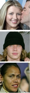
(i) Ours

Figure B.6: More qualitative comparison results on LFW-Test. (Zoom in for best view).

(a) LQ

(b) GPEN [37]

(c) GFPGAN [31]

(d) VQFR [9]

(e) RestoreFormer [34]

(f) SwinIR [19]

(g) DifFace [39]

(h) DR2 [35]

(i) Ours

Figure B.7: More qualitative comparison results on WebPhoto-Test. (Zoom in for best view).

(a) LQ

(b) GPEN [37]

(c) GFPGAN [31]

(d) VQFR [9]

(e) RestoreFormer [34]

(f) SwinIR [19]

(g) DifFace [39]

(h) DR2 [35]

(i) Ours

Figure B.8: More qualitative comparison results on WIDER-Test. (Zoom in for best view).

References

- Bulat et al. [2018] Adrian Bulat, Jing Yang, and Georgios Tzimiropoulos. To learn image super-resolution, use a gan to learn how to do image degradation first. In ECCV, 2018.
- Chen et al. [2021] Chaofeng Chen, Xiaoming Li, Lingbo Yang, Xianhui Lin, Lei Zhang, and Kwan-Yee K Wong. Progressive semantic-aware style transformation for blind face restoration. In CVPR, 2021.
- Chen et al. [2018] Yu Chen, Ying Tai, Xiaoming Liu, Chunhua Shen, and Jian Yang. FSRNet: End-to-end learning face super-resolution with facial priors. In CVPR, 2018.
- Chung et al. [2023] Hyungjin Chung, Jeongsol Kim, Michael Thompson Mccann, Marc Louis Klasky, and Jong Chul Ye. Diffusion posterior sampling for general noisy inverse problems. In ICLR, 2023.
- Deng et al. [2019a] Jiankang Deng, Jia Guo, Niannan Xue, and Stefanos Zafeiriou. Arcface: Additive angular margin loss for deep face recognition. In CVPR, 2019a.
- Deng et al. [2019b] Jiankang Deng, Anastasios Roussos, Grigorios Chrysos, Evangelos Ververas, Irene Kotsia, Jie Shen, and Stefanos Zafeiriou. The menpo benchmark for multi-pose 2d and 3d facial landmark localisation and tracking. IJCV, 2019b.
- Dhariwal and Nichol [2021] Prafulla Dhariwal and Alexander Nichol. Diffusion models beat gans on image synthesis. In NeurIPS, 2021.
- Esser et al. [2021] Patrick Esser, Robin Rombach, and Bjorn Ommer. Taming transformers for high-resolution image synthesis. In CVPR, 2021.
- Gu et al. [2022] Yuchao Gu, Xintao Wang, Liangbin Xie, Chao Dong, Gen Li, Ying Shan, and Ming-Ming Cheng. VQFR: Blind face restoration with vector-quantized dictionary and parallel decoder. In ECCV, 2022.
- Heusel et al. [2017] Martin Heusel, Hubert Ramsauer, Thomas Unterthiner, Bernhard Nessler, and Sepp Hochreiter. GANs trained by a two time-scale update rule converge to a local nash equilibrium. In NeurIPS, 2017.
- Ho et al. [2020] Jonathan Ho, Ajay Jain, and Pieter Abbeel. Denoising diffusion probabilistic models. In NeurIPS, 2020.
- Huang et al. [2008] Gary B Huang, Marwan Mattar, Tamara Berg, and Eric Learned-Miller. Labeled faces in the wild: A database for studying face recognition in unconstrained environments. Tech. Report, 2008.
- Karras et al. [2018] Tero Karras, Timo Aila, Samuli Laine, and Jaakko Lehtinen. Progressive growing of GANs for improved quality, stability, and variation. In ICLR, 2018.
- Karras et al. [2019] Tero Karras, Samuli Laine, and Timo Aila. A style-based generator architecture for generative adversarial networks. In CVPR, 2019.
- Karras et al. [2020] Tero Karras, Samuli Laine, Miika Aittala, Janne Hellsten, Jaakko Lehtinen, and Timo Aila. Analyzing and improving the image quality of stylegan. In CVPR, 2020.
- Kawar et al. [2022] Bahjat Kawar, Michael Elad, Stefano Ermon, and Jiaming Song. Denoising diffusion restoration models. In NeurIPS, 2022.
- Kingma and Ba [2015] Diederik P Kingma and Jimmy Ba. Adam: A method for stochastic optimization. In ICLR, 2015.
- Li et al. [2018] Xiaoming Li, Ming Liu, Yuting Ye, Wangmeng Zuo, Liang Lin, and Ruigang Yang. Learning warped guidance for blind face restoration. In ECCV, 2018.
- Liang et al. [2021] Jingyun Liang, Jiezhang Cao, Guolei Sun, Kai Zhang, Luc Van Gool, and Radu Timofte. SwinIR: Image restoration using swin transformer. In ICCV, 2021.
- Ma et al. [2017] Chao Ma, Chih-Yuan Yang, Xiaokang Yang, and Ming-Hsuan Yang. Learning a no-reference quality metric for single-image super-resolution. CVIU, 2017.
- Mittal et al. [2012] Anish Mittal, Rajiv Soundararajan, and Alan C Bovik. Making a “completely blind” image quality analyzer. SPL, 2012.
- Nichol and Dhariwal [2021] Alexander Quinn Nichol and Prafulla Dhariwal. Improved denoising diffusion probabilistic models. In ICML, 2021.
- Phung et al. [2023] Hao Phung, Quan Dao, and Anh Tran. Wavelet diffusion models are fast and scalable image generators. In CVPR, 2023.
- Preechakul et al. [2022] Konpat Preechakul, Nattanat Chatthee, Suttisak Wizadwongsa, and Supasorn Suwajanakorn. Diffusion autoencoders: Toward a meaningful and decodable representation. In CVPR, 2022.
- Rombach et al. [2022] Robin Rombach, Andreas Blattmann, Dominik Lorenz, Patrick Esser, and Björn Ommer. High-resolution image synthesis with latent diffusion models. In CVPR, 2022.
- Saharia et al. [2022] Chitwan Saharia, Jonathan Ho, William Chan, Tim Salimans, David J Fleet, and Mohammad Norouzi. Image super-resolution via iterative refinement. TPAMI, 2022.
- Shen et al. [2018] Ziyi Shen, Wei-Sheng Lai, Tingfa Xu, Jan Kautz, and Ming-Hsuan Yang. Deep semantic face deblurring. In CVPR, 2018.
- Song et al. [2020] Jiaming Song, Chenlin Meng, and Stefano Ermon. Denoising diffusion implicit models. arXiv:2010.02502, 2020.
- Vaswani et al. [2017] Ashish Vaswani, Noam Shazeer, Niki Parmar, Jakob Uszkoreit, Llion Jones, Aidan N Gomez, Łukasz Kaiser, and Illia Polosukhin. Attention is all you need. In NeurIPS, 2017.
- Wang et al. [2022a] Tao Wang, Kaihao Zhang, Xuanxi Chen, Wenhan Luo, Jiankang Deng, Tong Lu, Xiaochun Cao, Wei Liu, Hongdong Li, and Stefanos Zafeiriou. A survey of deep face restoration: Denoise, super-resolution, deblur, artifact removal. arXiv:2211.02831, 2022a.
- Wang et al. [2021a] Xintao Wang, Yu Li, Honglun Zhang, and Ying Shan. Towards real-world blind face restoration with generative facial prior. In CVPR, 2021a.
- Wang et al. [2021b] Xintao Wang, Liangbin Xie, Chao Dong, and Ying Shan. Real-esrgan: Training real-world blind super-resolution with pure synthetic data. In ICCV Workshops, 2021b.
- Wang et al. [2004] Zhou Wang, Alan C Bovik, Hamid R Sheikh, and Eero P Simoncelli. Image quality assessment: from error visibility to structural similarity. TIP, 2004.
- Wang et al. [2022b] Zhouxia Wang, Jiawei Zhang, Runjian Chen, Wenping Wang, and Ping Luo. Restoreformer: High-quality blind face restoration from undegraded key-value pairs. In CVPR, 2022b.
- Wang et al. [2023] Zhixin Wang, Ziying Zhang, Xiaoyun Zhang, Huangjie Zheng, Mingyuan Zhou, Ya Zhang, and Yanfeng Wang. DR2: Diffusion-based robust degradation remover for blind face restoration. In CVPR, 2023.
- Yang et al. [2016] Shuo Yang, Ping Luo, Chen-Change Loy, and Xiaoou Tang. Wider face: A face detection benchmark. In CVPR, 2016.
- Yang et al. [2021] Tao Yang, Peiran Ren, Xuansong Xie, and Lei Zhang. Gan prior embedded network for blind face restoration in the wild. In CVPR, 2021.
- Yu et al. [2018] Xin Yu, Basura Fernando, Bernard Ghanem, Fatih Porikli, and Richard Hartley. Face super-resolution guided by facial component heatmaps. In ECCV, 2018.
- Yue and Loy [2022] Zongsheng Yue and Chen Change Loy. Difface: Blind face restoration with diffused error contraction. arXiv:2212.06512, 2022.
- Zhang et al. [2022] Kaihao Zhang, Dongxu Li, Wenhan Luo, Jingyu Liu, Jiankang Deng, Wei Liu, and Stefanos Zafeiriou. Edface-celeb-1 m: Benchmarking face hallucination with a million-scale dataset. TPAMI, 2022.
- Zhang et al. [2018] Richard Zhang, Phillip Isola, Alexei A Efros, Eli Shechtman, and Oliver Wang. The unreasonable effectiveness of deep features as a perceptual metric. In CVPR, 2018.
- Zheng et al. [2022] Qingping Zheng, Jiankang Deng, Zheng Zhu, Ying Li, and Stefanos Zafeiriou. Decoupled multi-task learning with cyclical self-regulation for face parsing. In CVPR, 2022.
- Zhou et al. [2022] Shangchen Zhou, Kelvin Chan, Chongyi Li, and Chen Change Loy. Towards robust blind face restoration with codebook lookup transformer. In NeurIPS, 2022.