Robust Numerical Methods for Nonlinear Regression

Abstract

Many scientific and engineering applications require fitting regression models that are nonlinear in the parameters. Advances in computer hardware and software in recent decades have made it easier to fit such models. Relative to fitting regression models that are linear in the parameters, however, fitting nonlinear regression models is more complicated. In particular, software like the nls R function requires care in how the model is parameterized and how initial values are chosen for the maximum likelihood iterations. Often special diagnostics are needed to detect and suggest approaches for dealing with identifiability problems that can arise with such model fitting. When using Bayesian inference, there is the added complication of having to specify (often noninformative or weakly informative) prior distributions. Generally, the details for these tasks must be determined for each new nonlinear regression model. This paper provides a step-by-step procedure for specifying these details for any appropriate nonlinear regression model. Following the procedure will result in a numerically robust algorithm for fitting the nonlinear regression model. We illustrate the methods with three different nonlinear models that are used in the analysis of experimental fatigue data and we include two detailed numerical examples.

Keywords:  Bayesian, Fatigue, Maximum likelihood, Noninformative prior, Reparameterization, Stable parameters

1 Introduction

1.1 Background and motivation

Numerically robust algorithms for estimating the parameters of nonlinear regression models, using nonlinear least squares (NLS), maximum likelihood (ML) or Bayesian estimation, require

• Careful attention to parameterization.

• Methods for finding “initial values” for the parameters to start iterative estimation algorithms.

• Diagnostics for detecting estimability problems when the data are not sufficient to estimate the model parameters (e.g., trying to fit a four-parameter curvilinear relationship when there is not sufficient curvature in the data).

• When doing Bayesian estimation, default noninformative or weakly informative priors.

Over many years in many application areas, we have had experiences in which we developed and used the methods given in this paper to produce robust computational algorithms across a wide range of different kinds of nonlinear statistical models. The motivation to write this paper came from recent work to develop the robust numerical methods for the nonlinear regression models used in the applications in Meeker et al. (2024). The methods presented here, however, are broadly applicable for many other application areas where nonlinear estimation is used. Some other examples that have been documented are described in Meeker et al. (2022, Chapters 10, 20, 21, and 22) and Tian et al. (2024).

1.2 Other related literature

Before computers became widely available to researchers, nonlinear regression models were rarely used in practice. Starting in the late 1960s, rapid progress began. In pioneering work, Ross (1970) showed the importance studying the analytical properties of a nonlinear model and its relationship to the data. Doing so helps to formulate numerically robust estimation algorithms that have a much higher probability of successfully completing the estimation task. His ideas were extended and described, along with many additional examples in Ross (1990). The ideas of Ross have had a strong effect on the methods we have developed and refined.

Other books on nonlinear regression from around the same time include Ratkowsky (1983), Gallant (1987), Bates and Watts (1988), and Seber and Wild (1989). More recently, Huet et al. (2004) use a large number of example applications to illustrate the use of the nls2 R package to fit nonlinear regression models. Nash (2014) reviews methods of nonlinear estimation with emphasis on the mathematical programming aspects of solving NLS or ML estimation problems.

1.3 Overview

The rest of this paper is organized as follows. Section 2 outlines the general strategy for developing a numerically robust estimation procedure. Section 3 provides a brief introduction to linear and nonlinear regression models used to describe experimental fatigue data. We use nonlinear regression models from this area to illustrate the application of the main ideas presented in this paper. Section 4 provides implementation details for the Coffin–Manson nonlinear regression model. Sections 5 and 6 do the same for the Nishijima and Box–Cox/Loglinear-$\sigma_{N}$ models, respectively. Section 7 contains numerical examples that illustrate the methods. Section 8 provides some concluding remarks and suggests areas for related future research.

2 The General Strategy

This section outlines our general strategy for developing robust numerical methods for fitting nonlinear regression models. Our focus is on models that have a single explanatory variable, but all of the ideas extend directly to models with more than one explanatory variable. Briefly, from many years of experience, we have found that numerically robust nonlinear estimation algorithms can be developed by using a good parameterization and having good initial values for the estimation algorithm.

As suggested in the previous paragraph, a key component of our strategy is to carefully choose a parameterization for a statistical model. Proposed linear and nonlinear regression models are often written in a form where one or more of the traditional parameters (hereafter, the TPs) have no practical interpretation and may have one or more high correlations between parameters; such parameters can be “unstable.” An example is the intercept of the simple linear regression model that is far removed from the data. One effect of such a poor parameterization (beside lack of practical interpretability of the intercept) is that the estimates of the slope and intercept can be highly correlated (and thus relatively unstable). The common remedy for this particular deficient parameterization (a remedy that is also useful in other regression applications) is to center the explanatory variable which, in effect, redefines the intercept to be at the center of the data.

Sections 4–6 provide technical details for the suggested scaling and parameterization for the three example nonlinear regression models. Section 7 provides two numerical examples that illustrate the ML and data analysis steps of the procedures described in this section.

Table 1: Acronyms used in this paper

cdf		Cumulative distribution function
pdf		Probability density function
ML		Maximum likelihood
NLS		Nonlinear least squares
TP		Traditional parameter based on scaled data
SP		Stable parameter
USP		Unrestricted stable parameter
TPNS		Traditional parameter if data had not been scaled
S-N		Stress and number of cycles

2.1 Steps for ML estimation

Even when the final goal is Bayesian inference, we find it useful (for reasons described in Section 2.2) to start with ML estimation. We use ML instead of NLS because ML is more general. It provides a statistically correct method for handling the right-censored observations (known as “runouts” in the fatigue literature) and distributions other than the normal distribution that are commonly seen in many applications. Thus, whether doing ML or Bayesian estimation, we start with the following procedures for ML estimation.

1. Scale both the response and the explanatory variables. Dividing the values of each variable by the largest values of each variable generally works well. This will ensure that the performance of the estimation algorithms will not depend on the units of the variables and avoids numerical problems that might arise (e.g., with the Box–Cox model in Section 6) when large numbers are raised to a large negative power.

2. Identify “stable parameters” (SPs) (as defined by Ross, 1970, 1990) that will not be highly correlated and that can be identified from available data. Seber and Wild (1989, in Chapters 3 and 4) also describe the importance of parameterization in nonlinear regression. For example, parameters that can be identified as features of the data in a plot of the model fitted to data will often be stable.

   Because appropriate SPs are not unique and can be usefully defined in different ways, finding such SPs is as much art as science and often requires some trial-and-error experimentation for a particular model by using a collection of typical data sets. One criterion is to choose an SP definition that results in low estimated correlations obtained from the estimated SPs variance-covariance matrix. The choice among different definitions for SPs usually is not critical but we have found that by experimenting with a benchmark collection of data sets (some of which might have been simulated) allows comparison among alternative SP definitions.

   It is appealing to have SPs that are interpretable (and usually they are, almost by definition, if they can be identified as features of the data in a plot). Also, when Bayesian methods are to be used, SPs will generally simplify prior specification and elicitation from subject-matter experts because such parameters typically have an easy-to-understand interpretation and have estimates that tend not to be highly correlated.

   It is possible for the SPs to depend on the available data. For example, Meeker et al. (2022, Chapter 10) and Tian et al. (2024, Section 3.2) suggest using a distribution quantile (to replace the usual scale parameter) as an SP when fitting log-location-scale distributions to censored data. The particular quantile that should be used depends on the amount of censoring in the data. In two of the examples in this paper, we use points on the fitted model that are chosen to be within the range of the data as SPs.

3. If needed, further transform the SPs so that they do not have limits depending on other parameters and are unrestricted (e.g., take logs of positive parameters). Most estimation algorithms (ML or Bayesian MCMC) perform better when parameters are unrestricted. For clarity and consistency, we call these parameters the “unrestricted stable parameters” (USPs) although they could also be called the “estimation parameters” because they are the parameters that the estimation/optimization algorithm sees. An important consideration in the definition of SPs and USPs is that there should be an easy way to compute the TPs as a function of the USPs.

4. Initial values are needed to start ML iterations and MCMC algorithms. Recall that SPs can often be thought of as features that can be identified from plots of the data. Usually initial values can be obtained by using simple descriptive statistics or moment estimates (e.g., sample means, variances, and ordinary least squares), ignoring any censoring or other complicated features of the data. Especially when using a stable parameterization, the initial values to start ML estimation do not have to be close to the maximum of the likelihood. When the likelihood is well behaved (i.e., when the likelihood is expressed in terms of stable parameters and when the maximum of the likelihood is unique), initial values only need to be in the region where the likelihood is nonnegligible.

   In situations where the likelihood has multiple maxima (usually one global maximum with one or more local maxima at lower levels of relative likelihood), a more elaborate approach is needed. For example, it may be necessary to perform the optimization with many systematically or randomly chosen start values. Generally, however, it is best to understand the reason and interpretation of the multiple maxima (e.g., such multiple maxima may suggest an over-parameterized model). We illustrate this in one of our examples in Section 7.2.

5. Attempt the ML estimation. Check the results by computing the gradient vector (the elements should be close to zero) and the Hessian matrix (the eigenvalues should all be negative) of the log-likelihood evaluated at the maximum. We have found that (especially because we work with USPs) the needed derivatives can be computed by using carefully programmed finite differences (e.g., Barton, 1992).

6. When the estimation diagnostics indicate that convergence has not been successful, the particulars (e.g., the eigenvector corresponding to the smallest eigenvalue of the Hessian matrix) will generally provide signatures indicating what caused the problem and that, in turn, will suggest how to proceed (e.g., by fixing a parameter, switching to a particular submodel, a limiting model, or some other alternative well-fitting model, perhaps with fewer parameters).

7. To check for estimability and as a diagnostic to help understand the root-causes of estimation problems, especially in situations with a new model and a new kind of data, it is important to examine profile relative likelihood plots for individual parameters (one-dimensional profiles) and parameter pairs (two-dimensional profiles). The examples in Sections 7.1 and 7.2 illustrate the use of such profiles.

8. Translate the USP ML estimates back to ML estimates of the TPs that users would have obtained if without reparameterization (and if there were no numerical problems). Also obtain the variance-covariance matrix for the TPs using the vector version of the delta method (e.g., Section C.2 of Meeker et al., 2022).

9. Use the estimation results to do the usual residual analysis to assess how well the fitted model agrees with the data.

10. Translate the TP ML parameter estimates back to ML estimates of the unscaled TPs (which we call the TPNSs) that users would have obtained if unscaled data had been used (and if there were no numerical problems). Also obtain the corresponding variance-covariance matrix for the TPNSs.

11. In our software, we use the TP estimates (not the TPNS parameter estimates) to compute point estimates and confidence intervals for needed functions of the parameters such as distribution quantiles or cdf tail probabilities. Using the TP estimates protects against numerical problems that might occur when using the TPNSs. Parameter estimation results reported to users, however, are always unscaled (i.e., the TPNSs as if the data had not been scaled). Users of the software generally have no need to know about the details of how the scaling was done.

12. To develop numerically robust algorithms for particular models, it is important to employ “stress tests” by collecting, simulating, or otherwise generating a benchmark collection of data sets designed to challenge the algorithms. Testing on such a collection of data sets helps to develop appropriate diagnostic checks to trap potential estimation problems (e.g., when the level of a profile likelihood is non-zero for extreme values (i.e., $\pm\infty$) of one or more of the USPs).

2.2 Steps for Bayesian prior specification and estimation

If continuing on to Bayesian estimation, we again use the USPs as estimation parameters and suppose that there is a desire or need to use noninformative or weakly informative prior distributions. Then we use the following steps to obtain default prior distributions, MCMC initial values, and posterior draws via an MCMC engine. In this paper we take the modern applied approach (also see the rejoinder for the discussion in Tian et al., 2024) and treat the MCMC engine as a black box. The justification for doing this in our class of problems (models with at most a moderate number of parameters and the number of parameters does not depend on the data) is that with properly-defined USPs and confidence that all parameters are estimable, a reasonable MCMC algorithm (e.g., programing our USP model in Stan) should complete successfully.

In all cases, it is important to carefully examine MCMC diagnostics (especially trace plots for three or four independently drawn chains and corresponding numerical summaries) and check the adequacy of the fit to the data.

1. With typical S-N data sets (which contain much information about the parameters of the S-N relationship), there is little or no risk of encountering an improper posterior distribution. Thus using flat (i.e., uniform over the entire real line) marginal priors for each of the USPs provides a natural default joint prior distribution for the USPs defined in Step 3 of Section 2.1. In many cases, the flat prior for the USP will provide a good approximation to a reference prior (e.g., Berger and Bernardo, 1992). A reference prior would be difficult to establish exactly because of the nonlinearity in some S-N relationships and right censoring typically seen at low levels of stress.

2. While the flat prior suggested in the previous step should work well for most model/data combinations (especially if the data/model combination provided valid ML estimates), it is possible that the MCMC sampler could encounter difficulties (e.g., because the improper prior puts non-zero probability in nonsensical parts of the parameter space where the log-likelihood evaluations are in the noise of the numerical computations). In extreme cases, the posterior could be improper (e.g., when there is little information in the data about one or more parameters of the nonlinear regression model). In such cases, one can replace the flat marginal priors with approximately flat normal (Gaussian) distributions with a large standard deviation. Such an approximately noninformative (or weakly informative) prior will ensure that the posterior is proper but will not ensure that the MCMC sampler will accurately sample from the joint posterior distribution. We have encountered situations where the MCMC sampler finishes, the MCMC diagnostics look good, but the fitted model does not agree with the data (because “posterior draws” were being taken from one part of the approximately flat prior, far away from the likelihood). We have learned, however, that these problems are largely avoided if the USPs are defined well, as we will discuss within some of our particular numerical examples in Section 7.

3. When specifying a non-flat prior distribution (whether informative or weakly informative) we recommend using the “parameter-range” method (as used, for example, in Chapter 10 of Meeker et al., 2022) and Tian et al. (2024, Section 7.3) to specify a two-parameter marginal prior distribution (e.g., a normal distribution or a Student’s $t$ distribution with given degrees of freedom). Instead of specifying a marginal prior distribution and parameters of that distribution, specify instead the distribution and the 0.005 and 0.995 quantiles of the distribution as the “range” of the distribution. Such ranges are generally easier to elicit from subject-matter experts.

4. When flat or extremely wide normal distributions do not provide a satisfactory noninformative prior, it is necessary to use a weakly informative prior, usually represented by normal distributions with standard deviations that are not too large. To choose the mean and standard deviation of those normal distributions one can use information such as the scale of ones data, previous experience, and other engineering knowledge.

5. From our experience, having to specify weakly informative prior distributions in the manner described in Step 4 generally takes much time because it requires tedious trial-and-error. Thus (especially in software being designed to be user friendly) there is a need to automate the process of finding numerically-stable default noninformative or minimally informative priors. Technically, one should not use information from the data to help set the prior distribution (doing so violates the likelihood principle). For example, it would be a serious mistake to use 95% or even 99% confidence intervals from the data to choose a prior distribution parameter range (doing so is like using the available data twice!). Nevertheless, from a practical point of view, one can use the results of an ML estimation in a manner that can be shown to provide a prior distribution that is effectively noninformative and that avoids substantive reuse of one’s data.

   For example, if Wald-like approximate confidence intervals were computed using a factor of 20 standard errors instead of 1.96, the prior would be approximately flat over the part of the parameter space and somewhat beyond where the likelihood is nonnegligible. Weakly informative priors chosen in this way should be insensitive to the exact values of the mean and standard deviations of the specified normal distributions and this can be checked by doing sensitivity analysis (e.g., by generating a few hundred joint posterior draws and comparing for different settings of the prior-specification algorithm). For a similar view (but a somewhat different approach), see the vignette for the rstanarm R package in Gabry and Goodrich (2020).

6. Following common practice, we run four independent chains so that we can use standard MCMC diagnostics to check for convergence. We have found that MCMC initial values obtained by sampling randomly, without replacement, from the vertices of a hyper-rectangle defined by the endpoints of 95% confidence intervals for the parameters works well. Doing this improves the chances that MCMC sampling will be from the joint posterior instead of some alternative low-level island of probability elsewhere in the parameter space.

7. After draws from the posterior of the USPs have been computed and checked, similar to what is suggested in Step 11 in Section 2.1, compute and save posterior draws for the marginal distributions of the TPs (along with meta information on how the data were scaled to ensure that final results are reported correctly in terms what would have been computed by using the unscaled data). These can be used for post processing of the results to compute estimates and credible intervals for quantities of interest and make corresponding plots. For reasons of numerical stability when doing the post processing, it is better to not to convert these draws back to the TPs for the unscaled data (i.e., back to the TPNS).

3 A Brief Introduction to Modern Statistical Models for Experimental Fatigue Data

Because of its importance in areas such as aerospace, implantable medical device, automotive, and civil infrastructure engineering, fatigue is the most thoroughly studied failure mode in reliability. Engineers routinely conduct laboratory life tests, subjecting material specimens to cyclic stresses that induce the initiation and progression of cracks or other forms of damage. Experiments typically test samples of units as several fixed levels of stress amplitude (other experimental variables like mean stress or temperature are sometimes also used, but such extensions—which are straightforward to handle statistically—are not considered in this paper). Units are tested until failure (defined in some purposeful manner such as specimen fracture) or the end of the test. Unfailed units result in right-censored observations (known as runouts in the fatigue literature).

This section briefly reviews the statistical models used in Meeker et al. (2024) and that we use for applications in this paper. Section 3.1 describes S-N (stress or strain $S$ versus number of cycles to failure $N$) relationships. Section 3.2 reviews models for fatigue S-N data that use the traditional method of specifying a fatigue-life model. The specified fatigue-life model then induces a fatigue-strength model, as described more fully in Meeker et al. (2024, Section 2). Section 3.3 reviews models for fatigue S-N data that use a new method of specifying a fatigue-strength model which then induces a fatigue-life model, as described more fully in Meeker et al. (2024, Section 3). This new approach to S-N model specification has important advantages in applications where nonlinear regression is needed.

3.1 S-N relationships

A specified S-N regression relationship is the core component of any statistical model used to describe experimental fatigue data. This relationship describes how some quantile (usually the median) of the fatigue-life distribution is affected by stress. Usually, the relationship is specified in terms of a positive monotonically decreasing function $N=g(S;\boldsymbol{\beta})$, relating median number of cycles $N$ to stress amplitude $S$. The function must be monotonically decreasing because increasing stress tends to lead to shorter lifetimes. The vector $\boldsymbol{\beta}$ contains regression coefficients to be estimated from the available fatigue data. Numerous nonlinear S-N relationships have been suggested in the fatigue literature. Some of these are reviewed, for example, in Castillo and Fernández-Canteli (2009) and Meeker et al. (2024).

As explained in Dowling et al. (2020, Chapters 9 and 15), some fatigue experiments (depending on material properties and the levels of stress used in the experiment) are stress-controlled while others are strain-controlled. To simplify the presentation we will generally use the word “stress” to mean stress amplitude or strain amplitude used as the experimental factor in a fatigue experiment. An exception will be in Section 7.1 when we present the Inconel 718 example where strain amplitude was controlled.

The simplest S-N relationship in known as the Basquin relationship

$$\log(N) =\log[g(S;\boldsymbol{\beta})]=\beta_{0}+\beta_{1}\log(S),$$ (1)

given by Basquin (1910) where log life ($\log(N$) tends to be linear in log stress ($\log(S)$) and $\beta_{1}<0$. In application areas other than fatigue (e.g., accelerated life testing), this relationship is known as the inverse power law.

More generally, the function $g(S;\boldsymbol{\beta})$, for fixed $\boldsymbol{\beta}$, needs to be a positive monotonically decreasing because the lifetime $N>0$ tends to decrease as stress $S>0$ increases. In some settings (as described in Section 3.3) it is either convenient or necessary to use instead the S-N relationship $S=h(N;\boldsymbol{\beta})=g^{-1}(N;\boldsymbol{\beta})$ which, for fixed $\boldsymbol{\beta}$, is a positive monotonically decreasing function of $N$. Especially in high-cycle fatigue tests (where units are tested at lower levels of stress and fatigue life times tend to be long), there can be strong curvature (usually, but not always the curvature is concave-up over the range of the data) in the S-N relationship, requiring the use of nonlinear regression models. The models used in Sections 4–6 illustrate such nonlinear regression relationships.

3.2 Specifying the fatigue-life model

When specifying a model for fatigue life $N$ at a specified level of stress $S_{e}$, we write

$$\log(N) =\log[g(S_{e};\boldsymbol{\beta})]+\sigma_{N}\epsilon.$$

Here $\sigma_{N}\epsilon$ is a random-error term where $\epsilon$ has a location-scale distribution with $\mu=0$ and $\sigma=1.$ Then for a given level of stress amplitude $S_{e}$, the cdf of $N$ is

$$F_{N}(t;S_{e}) =\Pr\left(N\leq t;S_{e}\right)=\Phi\left(\frac{\log(t)-\log[g(S_{e};\boldsymbol{\beta})]}{\sigma_{N}}\right),\quad\quad t>0,\,\,S_{e}>0,$$ (2)

which is a log-location-scale distribution with scale parameter $g(S_{e};\boldsymbol{\beta})>0$ and shape parameter $\sigma_{N}$. The log-location-scale family of distributions includes the widely used (for fatigue and other applications involving time-to-event data) lognormal and Weibull distributions as special cases.

“Fatigue strength” (which is sometimes referred to as “fatigue resistance”) is a random variable, denoted by $X$, giving the level of stress that leads to a failure at a specified number of cycles $N_{e}$. Using this definition of $X$ implies that the models for the random variables $N$ and $X$ have the same random component $\epsilon$. Although $X$ cannot be directly observed, the distribution of $X$ can be estimated from S-N data. We note that in the fatigue literature, there are alternative definitions of fatigue strength, but the one we use is the most common one.

As shown in Meeker et al. (2024, Section 2.4.1), for the specified log-location-scale fatigue-life model in (2), the above definition of $X$ implies (when $g(S_{e};\boldsymbol{\beta})$ has neither a vertical nor a horizontal asymptote) that the cdf of $X$ is

$$F_{X}(x;N_{e}) =\Pr\left(X\leq x;N_{e}\right)=\Phi\left[\frac{\log(N_{e})-\log[g(x;\boldsymbol{\beta})]}{\sigma_{N}}\right],\quad\quad x>0,\,\,N_{e}>0.$$ (3)

If $N=g(S;\boldsymbol{\beta})$ has one or both coordinate asymptotes, technical adjustments are needed to define the cdf, as described in Meeker et al. (2024, Sections 2.4.2 and 2.4.3). The cdf in (3) is not a log-location-scale distribution unless $\log[g(x;\boldsymbol{\beta})]$ is a linear function of $\log(x)$ (i.e., the Basquin relationship).

3.3 Specifying the fatigue-strength model

As an alternative to the traditional method of specifying a fatigue-life model (that will then induce a fatigue-strength model for the random variable $X$), Meeker et al. (2024, Section 3.2) suggest specifying a fatigue-strength model for $X$ that will then induce a fatigue-life model for $N$. The biggest advantage (described more fully in Meeker et al., 2024, Section 3.2.1) of this new approach is that the specification of the fatigue strength model is simpler in the frequently occurring applications where the S-N relationship is nonlinear on log-log scales. In particular, the fatigue-life distribution often has increasing spread at lower levels of stress $S$; the fatigue-strength distributions typically have a constant spread as a function of number of cycles $N_{e}$.

To specify a fatigue-strength distribution, let

$$\log(X)=\log[h(N_{e};\boldsymbol{\beta})]+\sigma_{X}\epsilon,$$ (4)

where $S=h(N;\boldsymbol{\beta})$ defines the S-N regression relationship. Then $\sigma_{X}\epsilon$ is a random-error term where $\epsilon$ has a location-scale distribution with $\mu=0$ and $\sigma=1.$ This model implies that, for a given number of cycles $N_{e}$, $X$ has a cdf

$$F_{X}(x;N_{e}) =\Pr(X\leq x;N_{e})=\Phi\left[\frac{\log(x)-\log[h(N_{e};\boldsymbol{\beta})]}{\sigma_{X}}\right],\quad\quad x>0,\,\,N_{e}>0.$$

Then $X$ has a log-location-scale distribution with scale parameter $h(N_{e};\boldsymbol{\beta})>0$ and constant shape parameter $\sigma_{X}$.

As shown in Meeker et al. (2024, Section 3.2.3), when the monotonically decreasing $S=h(N;\boldsymbol{\beta})$ has neither a vertical nor a horizontal asymptote, this model implies that fatigue-life $N$, for a given value of stress $S_{e}$, has the cdf

$$F_{N}(t;S_{e}) =\Pr(N\leq t;S_{e})=\Phi\left[\frac{\log(S_{e})-\log[h(t;\boldsymbol{\beta})]}{\sigma_{X}}\right],\quad\quad t>0,\,\,S_{e}>0.$$ (5)

If $S=h(N;\boldsymbol{\beta})$ has one or both coordinate asymptotes, technical adjustments are needed to define the cdf, as described in Meeker et al. (2024, Sections 3.2.4 and 3.2.5). The cdf in (5) is not a log-location-scale distribution unless $\log[h(t;\boldsymbol{\beta})]$ is a linear function of $\log(t)$ (i.e., the Basquin relationship).

Because $N$ is observable (and $X$ is not), we use the distribution of $N$ (in either (2) or (5)) to define the likelihood when fitting an S-N model to S-N data. When needed, pdfs for either situation are obtained by using $f_{N}(t;S_{e})=dF_{N}(t;S_{e})/dt$.

3.4 Scaling the data

As suggested in Step 1 in Section 2.1, it is useful and sometimes important to scale data before doing estimation. In our examples involving S-N data, we scale both the stress/strain variable $S$ and the response variable $N$. Dividing all values of $S$ and $N$ by the largest values of these variables (denoted by $S_{\max}$ and $N_{\max}$, respectively) generally works well.

3.5 Potential estimability problems

Section 2.1 mentioned the important concept of SPs. Sections 4–6 provide, as examples, the details the parameterizations that we tailored for the three five-parameter models that we have used in this paper. Although it is not a strict requirement for S-N relationships, most S-N data, especially when at least some units are tested at low levels of stress, have concave-up curvature and increased spread at lower levels of stress; the models used in Sections 4–6 usefully describe such data. In situations where the data plotted on log-log scales are approximately linear (e.g., low-cycle fatigue where all units are exposed to relatively high levels of stress), the Basquin relationship (1) may be appropriate.

In other model/data combinations, attempting to fit a more complicated model could lead to situations (depending on the model and definition of the USPs) where the maximum of the likelihood is at or near a boundary of the parameter space or the maximum may not be unique (due to flatness in the likelihood or profile likelihood surface). We have designed algorithms to detect such situations (somewhat tailored for each model) and provide suitable warnings. In such situations, one should attempt to fit the indicated limiting model (i.e., a model implied by one of the USPs approaching $\infty$ or $-\infty$) or other special-case models (such as the Basquin model) and carefully check model-fitting diagnostics (e.g., based on the residuals) to ensure that the model is adequate. The nested model (implied by a limiting case of the original model) can be compared with the original model by using a likelihood-ratio test (as described in Meeker et al., 2022, Appendix C.7.5). We illustrate some of these situations in our numerical examples in Sections 7.1 and 7.2.

4 Application of the Procedure for the Coffin–Manson Model

4.1 The Coffin–Manson model

The Coffin–Manson relationship (e.g., Dowling et al., 2020, pages 724–726) is a popular relationship for S-N data that exhibit, when plotted, concave-up curvature. The relationship, depicted in Figure 1(a), can be interpreted as the sum of plastic and elastic Basquin S-N relationships and is expressed as:

$$S=h(N;\boldsymbol{\beta})=A_{\textrm{el}}(2N)^{b}+A_{\textrm{pl}}(2N)^{c},$$ (6)

where the TPs are $A_{\textrm{el}}>0$, $A_{\textrm{pl}}\geq 0$, $b\leq 0$, $c<0$, and $|c|>|b|$. The last inequality makes the model identifiable. It is traditional to use $2N$ in (6) because there are two stress within each extremes cycle.

(a)	(b)

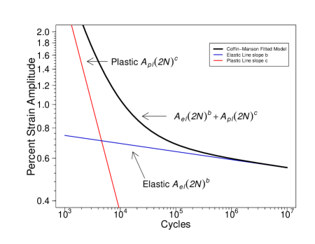
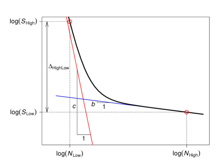
Figure 1: Plot showing the Coffin–Manson S-N relationship (a); Plot illustrating the Coffin–Manson USPs (b).

4.2 Coffin–Manson model SPs and USPs

As mentioned in Section 2.1, one way to identify SPs is to use model characteristics that can be easily identified from a plot of the fitted model. The dark solid curve in Figure 1(b) is a fitted Coffin–Manson relationship (the data have been suppressed in the plot). The figure also illustrates several quantities that provide the basis for our USPs.

Our Coffin–Manson SPs start with the stress levels $S_{\textrm{Low}}$ and $S_{\textrm{High}}$ that correspond to the two extreme points on the fitted S-N curve in Figure 1(b). These values can be computed from the TPs by using

$$\begin{split}S_{\textrm{Low}}&=A_{\textrm{el}}(2N_{\textrm{High}})^{b}+A_{\textrm{pl}}(2N_{\textrm{High}})^{c}\\ S_{\textrm{High}}&=A_{\textrm{el}}(2N_{\textrm{Low}})^{b}+A_{\textrm{pl}}(2N_{\textrm{Low}})^{c},\end{split}$$ (7)

where $N_{\textrm{High}}$ is the largest value of $N$ in the data that is a failure and $N_{\textrm{Low}}$ is the smallest value of $N$ in the data. We also use the elastic-line slope $b$ and the plastic-line slope $c$ as SPs. The vertical spread in the data points about the fitted model provides an indication of the value of $\sigma_{X}$ and thus $\sigma_{X}$ is an SP (even though fatigue strength $X$ is not directly observable and applied stress $S$ is an experimental factor, the vertical spread in the S-N data provides an indication of the spread in distribution of fatigue strength).

The SPs have the following constraints and order restrictions:

• $S_{\textrm{High}}>S_{\textrm{Low}}>0$,

• $c<\kappa<b<0$, and

• $\sigma_{X}>0$,

where

$$\begin{split}\kappa&=\frac{\log(S_{\textrm{Low}})-\log(S_{\textrm{High}})}{\log(N_{\textrm{High}})-\log(N_{\textrm{Low}})}\end{split}$$ (8)

is the slope of the line that connects the two open-circle points in Figure 1(b). Our corresponding USPs are

$$\begin{split}&\log\!S_{\textrm{Low}}=\log(S_{\textrm{Low}})\\ &\log\!\Delta_{\textrm{SHigh}\textrm{SLow}}=\log[\log(S_{\textrm{High}})-\log(S_{\textrm{Low}})]\\ &\textrm{qlogis}p=\texttt{qlogis}(b/\kappa)\\ &\log\!\Delta_{\textrm{Slopes}}=\log\left(\kappa-c\right),\textrm{ and}\\ &\log\!\sigma_{X}=\log(\sigma_{X}),\end{split}$$ (9)

where qlogis is the standard logistic distribution quantile function (also known as the logit transformation).

The order restrictions $c<\kappa<b$ ensure that the resulting model is concave-up (and, correspondingly, that $A_{\textrm{el}}$ and $A_{\textrm{pl}}$ will be positive). Analytically, this can be seen as follows. The solutions of (7) for $A_{\textrm{el}}$ and $A_{\textrm{pl}}$ are:

$$\begin{split}A_{\textrm{el}}&=\dfrac{S_{\textrm{Low}}/(2N_{\textrm{High}})^{c}-S_{\textrm{High}}/(2N_{\textrm{Low}})^{c}}{(2N_{\textrm{High}})^{b-c}-(2N_{\textrm{Low}})^{b-c}}\\ A_{\textrm{pl}}&=\dfrac{S_{\textrm{Low}}/(2N_{\textrm{High}})^{b}-S_{\textrm{High}}/(2N_{\textrm{Low}})^{b}}{(2N_{\textrm{High}})^{c-b}-(2N_{\textrm{Low}})^{c-b}}.\end{split}$$ (10)

In (10), because $N_{\textrm{High}}>N_{\textrm{Low}}$ and $c<b$, the denominator of the solution for $A_{\textrm{el}}$ is positive and the denominator of the solution for $A_{\textrm{pl}}$ is negative. Because both $A_{\textrm{el}}$ and $A_{\textrm{pl}}$ must be positive, the numerator of the solution for $A_{\textrm{el}}$ must be positive, and the numerator of the solution for $A_{\textrm{pl}}$ must be negative, as expressed in the following inequalities:

$$\begin{split}S_{\textrm{Low}}/(2N_{\textrm{High}})^{c}-S_{\textrm{High}}/(2N_{\textrm{Low}})^{c}&>0\\ S_{\textrm{Low}}/(2N_{\textrm{High}})^{b}-S_{\textrm{High}}/(2N_{\textrm{Low}})^{b}&<0.\end{split}$$ (11)

Solving (11) for $b$ and $c$ leads to the order restrictions $c<\kappa<b$ and the expression for $\kappa$ in (8).

4.3 Initial values for the Coffin–Manson USPs

Our algorithm determines initial values for the SPs first, then translates those initial values into initial values for the USPs. An optimization routine then finds the values of the USPs that maximize the likelihood function.

The initial value for $S_{\textrm{Low}}$ is the smallest stress value among all failure observations (i.e., omitting the right-censored observations). The initial value for $S_{\textrm{High}}$ is the largest stress value among all failure observations. The initial values for $b$ and $c$ are ordinary least squares (OLS) slope estimates of two simple linear regressions using two data subsets. The two data subsets are obtained by dividing the data into two groups (below and above the median lifetime) and treating right-censored observations as failures. For each data subset, a simple linear regression is fit using OLS using the logarithm of stress as the response variable and the logarithm of lifetime as the explanatory variable. The slope estimate from the subset with smaller lifetimes is the initial value for $c$, the elastic-line slope. The other slope estimate is for $b$, the plastic-line slope.

An initial value for $\sigma_{X}$ is obtained by using the residual standard deviation from an OLS fit, again using the logarithm of stress as the response variable and the logarithm of lifetime as the explanatory variable. This results in an estimate that is biased high, which we have found to be a robust initial value for $\sigma_{X}$. Then one computes the initial values of the USPs from (8) and (LABEL:equation:cm.unrestricted.stable.definition).

4.4 Computing the Coffin–Manson TPs from the USPs

The equations for the likelihood itself will usually be programmed in terms of the TPs. Before computing the likelihood, one then needs to compute the TPs from the USPs, usually by calling a function to do this at the very beginning of the function to compute the likelihood. Also, when estimation is complete there is need to compute the ML estimates of the TPs. The Coffin–Manson TPs as functions of our Coffin–Manson USPs are:

$$\begin{split}b&=\kappa\cdot\texttt{plogis}(\textrm{qlogis}p)\\[2.15277pt] c&=\kappa-\exp(\log\!\Delta_{\textrm{Slopes}})\\[2.15277pt] A_{\textrm{pl}}&=\dfrac{S_{\textrm{Low}}/(2N_{\textrm{High}})^{b}-S_{\textrm{High}}/(2N_{\textrm{Low}})^{b}}{(2N_{\textrm{High}})^{c-b}-(2N_{\textrm{Low}})^{c-b}}\\[2.15277pt] A_{\textrm{el}}&=\dfrac{S_{\textrm{High}}}{(2N_{\textrm{Low}})^{b}}-(2N_{\textrm{Low}})^{c-b}A_{\textrm{pl}}\\[2.15277pt] \sigma_{X}&=\exp(\log\!\sigma_{X}),\end{split}$$ (12)

where plogis is the standard logistic distribution cdf (also known as the inverse logit transformation),

$$S_{\textrm{Low}} =\exp(\log\!S_{\textrm{Low}})$$

$$S_{\textrm{High}} =\exp(\log\!S_{\textrm{Low}}+\exp[\log\!\Delta_{\textrm{SHigh}\textrm{SLow}}]),$$

and $\kappa$ is computed using (8).

4.5 ML estimates of the traditional parameters based on the original unscaled data

As described in Step 1 of Section 2.1, to ensure numerical stability, we use the scaled data to calculate the likelihood function as a function of the USPs. Thus the initial results of ML estimation provide ML estimates of the USPs based on the scaled data. To recover the ML estimates for TPs based on the scaled data, one uses (12).

To report final results the ML estimates of the TPs for the original unscaled data (which we call TPNSs) can be computed as follows. Denote the ML estimates for the TPs from the scaled data by $\widetilde{A}_{pl}$, $\widetilde{b}$, $\widetilde{A}_{el}$, and $\widetilde{c}$, where the scaling values are $S_{\max}$ and $N_{\max}$ respectively for stress and number of cycles. Then the fitted Coffin–Manson model for the scaled data is:

$$\widetilde{S}=\widetilde{A}_{\textrm{el}}(2\widetilde{N})^{\widetilde{b}}+\widetilde{A}_{\textrm{pl}}(2\widetilde{N})^{\widetilde{c}},$$

where $\widetilde{S}$ and $\widetilde{N}$ are scaled stress and lifetime values. In terms of the original data and scaling factor, the relationship is:

$$S=S_{\max}\widetilde{A}_{\textrm{el}}N_{\max}^{-\widetilde{b}}(2N)^{\widetilde{b}}+S_{\max}\widetilde{A}_{\textrm{pl}}N_{\max}^{-\widetilde{c}}(2N)^{\widetilde{c}}.$$

Therefore, the ML estimates for the TPNSs are:

$$\widehat{A}_{\textrm{el}} =S_{\max}\widetilde{A}_{\textrm{el}}N_{\max}^{-\widetilde{b}}$$

$$\widehat{A}_{\textrm{pl}} =S_{\max}\widetilde{A}_{\textrm{pl}}N_{\max}^{-\widetilde{c}}$$

$$\widehat{b} =\widetilde{b}$$

$$\widehat{c} =\widetilde{c}.$$

4.6 Coffin–Manson limiting cases and competing models

The Coffin–Manson model has two limiting cases that are plausible S-N-curve models. One is the Coffin–Manson Zero-Elastic-Slope model (where the elastic line becomes a horizontal asymptote), and the other is the Basquin model. In terms of TPs, when the parameter $b$ in (6) approaches zero, the Coffin–Manson model approaches the Coffin–Manson Zero-Elastic-Slope model. The limiting model has the following S-N relationship:

$$S=h(N;\boldsymbol{\beta})=A_{\textrm{el}}+A_{\textrm{pl}}(2N)^{c}.$$ (13)

The second limiting model is the Basquin model. When either $A_{\textrm{el}}\rightarrow 0$ or $A_{\textrm{pl}}\rightarrow 0$, (6) approaches the following S-N relationship:

$$S=h(N;\boldsymbol{\beta})=\textit{A}(2N)^{\kappa}.$$ (14)

after reparameterization, (1) and (14) are equivalent.

In terms of the USPs, when parameter $\texttt{qlogis}(p)\rightarrow-\infty$ the Coffin–Manson model approaches the Coffin–Manson Zero-Elastic-Slope model (13) (because $b\rightarrow 0$). When $\log(\delta)\rightarrow 0$ or $\texttt{qlogis}(p)\rightarrow\infty$ or both, the Coffin–Manson model approaches the Basquin model. This can be seen by letting $\log(\delta)\rightarrow 0$ which implies that $c\rightarrow\kappa$ and letting $\texttt{qlogis}(p)\rightarrow\infty$ which implies that $b\rightarrow\kappa$. Therefore, $A_{\textrm{pl}}\rightarrow 0$ or $A_{\textrm{el}}\rightarrow 0$, according to (10) and (11) in Section 4.2.

5 Application of the Procedure for the Nishijima Model

5.1 The Nishijima model

The Nishijima S-N relationship is described and used in Falk (2019) and Meeker et al. (2024). Although it is less well known than the Coffin–Manson model, the Nishijima model provides a good description of many S-N data sets. The Nishijima relationship is the hyperbola:

$$[\log(S)-E][\log(S)+A\log(N)-B] =C,$$ (15)

or equivalently

$$S =h(N;\boldsymbol{\beta})=\exp\left(\frac{-A\log(N)+B+E+\sqrt{\left[A\log(N)-(B-E)\right]^{2}+4C}}{2}\right),$$ (16)

depicted in Figure 2(a), where $A$, $B$, $C$, and $E$ (indicated on the plot) are the regression model TPs. The TPs have the constraints:

$$\begin{array}[]{cccc}&A&>&0,\\ &C&>&0.\end{array}$$

These constraints ensure that (16) is concave-up.

(a)	(b)

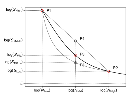
Figure 2: Plot showing the Nishijima S-N relationship (a); Plot illustrating the Nishijima USPs (b).

The parameter $A$ is the negative of slope of the oblique asymptote, $B$ is the $\log(N)=0$ intercept of the same asymptote, $E$ is the log of the horizontal asymptote, and $\sqrt{C}$ is the vertical distance between the S-N curve and the point where the two asymptotes intersect.

5.2 Nishijima model SPs and USPs

Similar to identifying model characteristics for the Coffin–Manson model, the stable parameterization for the Nishijima model can be observed from the plot of a fitted model, illustrated by Figure 2(b). The SPs of the Nishijima model consist of $S_{\textrm{High}}$, $S_{\textrm{Mid}}$, $S_{\textrm{Low}}$, $E$, and $\sigma_{X}$. The first three SPs, which replace the traditional $A$, $B$, and $C$, are stress levels that correspond to the three open-circle points (P1, P2, and P3) on the thick solid Nishijima S-N curve in Figure 2(b). These values can be computed from the traditional parameters, according to (16), by using the following three points on the Nishijima relationship:

$$\begin{split}S_{\textrm{Low}}&=h(N_{\textrm{High}};\beta)\\ S_{\textrm{Mid}}&=h(N_{\textrm{Mid}};\beta)\\ S_{\textrm{High}}&=h(N_{\textrm{Low}};\beta),\end{split}$$ (17)

where $N_{\textrm{Low}}$ is the smallest value of $N$ in the data, $N_{\textrm{High}}$ is the largest value of $N$ in the data that is a failure, and $N_{\textrm{Mid}}=\exp[(\log(N_{\textrm{Low}})+\log(N_{\textrm{High}}))/2]$ is the midpoint on the logarithmic scale.

The SPs have the following constraints and order restrictions:

• $0<\exp(E)<S_{\textrm{Low}}<S_{\textrm{Mid-L}}<S_{\textrm{Mid}}<S_{\textrm{Mid-U}}<S_{\textrm{High}}$, and

• $\sigma_{X}>0$,

where

$$\begin{split}\log(S_{\textrm{Mid-U}})&=\frac{1}{2}\,[\log(S_{\textrm{High}})+\log(S_{\textrm{Low}})]\\ \log(S_{\textrm{Mid-L}})&=2\,\frac{[\log(S_{\textrm{Low}})-E][\log(S_{\textrm{High}})-E]}{\log(S_{\textrm{Low}})+\log(S_{\textrm{High}})-2E}+E.\end{split}$$ (18)

The open-circles P3, P4, and P5 in Figure 2(b) have their horizontal position at $\log(N_{\textrm{Mid}})$. The stress values $S_{\textrm{Mid-U}}$ and $S_{\textrm{Mid-L}}$ give the vertical positions of the the open-circles P4 and P5. The open-circle P4 is at the middle of the line segment connecting P1 and P2, corresponding to the limiting linear S-N relationship. The open-circle P5 is on a curve that corresponds to the limiting rectangular hyperbola containing points P1 and P2 and having $E$ as its horizontal asymptote. The order restriction $S_{\textrm{Mid}}<S_{\textrm{Mid-U}}$ ensures that the Nishijima S-N curve is concave-up and can approach the linear S-N relationship between P1 and P2. The order restriction $S_{\textrm{Mid-L}}<S_{\textrm{Mid}}$ ensures that the Nishijima S-N curve is a hyperbola that can approach the limiting Rectangular Hyperbola S-N relationship. Section 5.6 describes both limits.

To derive the order restrictions $S_{\textrm{Mid-L}}<S_{\textrm{Mid}}<S_{\textrm{Mid-U}}$, start with the following equations:

$$\begin{split}-A\log(N_{\textrm{High}})+B+\frac{C}{\log(S_{\textrm{Low}})-E}&=\log(S_{\textrm{Low}})\\ -A\log(N_{\textrm{Mid}})+B+\frac{C}{\log(S_{\textrm{Mid}})-E}&=\log(S_{\textrm{Mid}})\\ -A\log(N_{\textrm{Low}})+B+\frac{C}{\log(S_{\textrm{High}})-E}&=\log(S_{\textrm{High}}).\end{split}$$ (19)

These equations are are obtained from (17). For example, to convert the first equation in (17) to the first equation in (19), use (15) to rewrite the first equation in (17) as follows:

$$[\log(S_{\textrm{Low}})-E][\log(S_{\textrm{Low}})+A\log(N_{\textrm{High}})-B] =C.$$ (20)

Then divide both sides by $[\log(S_{\textrm{Low}})-E]$ and move the terms involving $A$, $B$, $C$, and $E$ to the same side of the equation. Now add the first and the third equations in (19) together and subtract two times the second equation. The resulting equation simplifies because the terms involving $A$ and $B$ either cancel out or because $\log(N_{\textrm{Mid}})$ is the midpoint of the line between $\log(N_{\textrm{Low}})$ and $\log(N_{\textrm{High}})$. The final result is:

$$\log(S_{\textrm{Mid}})-\frac{1}{2}\left[\log(S_{\textrm{Low}})+\log(S_{\textrm{High}})\right] =C\left(\frac{1}{\log(S_{\textrm{Mid}})-E}-\frac{1}{2}\,\frac{\log(S_{\textrm{Low}})+\log(S_{\textrm{High}})-2E}{[\log(S_{\textrm{High}})-E][\log(S_{\textrm{Low}})-E]}\right).$$ (21)

The left hand side of (21) is negative because of $S_{\textrm{Mid}}<S_{\textrm{Mid-U}}$. Then because $C>0$,

$$\left(\frac{1}{\log(S_{\textrm{Mid}})-E}-\frac{1}{2}\,\frac{\log(S_{\textrm{Low}})+\log(S_{\textrm{High}})-2E}{[\log(S_{\textrm{High}})-E][\log(S_{\textrm{Low}})-E]}\right) <0.$$

After rearranging terms, one can see that $S_{\textrm{Mid-L}}<S_{\textrm{Mid}}$, where $S_{\textrm{Mid-L}}$ is given by the second equation in (18).

Because the SPs have order restrictions and constraints, the corresponding Nishijima USPs are

$$\begin{split}&\log\!S_{\textrm{Low}}=\log(S_{\textrm{Low}})\\ &\log\!\Delta_{\textrm{SHigh}\textrm{SLow}}=\log[\log(S_{\textrm{High}})-\log(S_{\textrm{Low}})]\\ &\textrm{qlogis}p=\texttt{qlogis}(p)\\ &\log\!\Delta_{\textrm{SLow}E}=\log[\log(S_{\textrm{Low}})-E]\\ &\log\!\sigma_{X}=\log(\sigma_{X}),\end{split}$$ (22)

where qlogis is the standard logistic distribution quantile function (also known as the logit transformation),

$$p =\frac{\log(S_{\textrm{Mid-U}})-\log(S_{\textrm{Mid}})}{\log(S_{\textrm{Mid-U}})-\log(S_{\textrm{Mid-L}})},$$

and $\log(S_{\textrm{Mid-L}})$ and $\log(S_{\textrm{Mid-U}})$ are computed from the other USPs using (18).

5.3 Initial values for the Nishijima USPs

The initial values for $S_{\textrm{Low}}$, $S_{\textrm{High}}$, and $\sigma_{X}$ are obtained in the same way as the Coffin–Manson for the SPs with the same names. For the other two SPs, we use:

$$E =\log(S_{\textrm{Low}})-0.1[\log(S_{\textrm{High}})-\log(S_{\textrm{Low}})]$$

$$S_{\textrm{Mid}} =\exp\left(\frac{1}{2}[\log(S_{\textrm{Mid-L}})+\log(S_{\textrm{Mid-U}})]\right),$$

where the formulas for $\log(S_{\textrm{Mid-L}})$ and $\log(S_{\textrm{Mid-U}})$ are given in (18). Then the initial values of USPs are calculated using (LABEL:equation:nishijima.unrestricted.stable.definition).

5.4 Computing the Nishijima TPs from the USPs

Similar to the Coffin–Manson model described in Section 4.4, the Nishijima TPs can be computed from the Nishijima USPs. First, compute Nishijima SPs from USPs by inverting the operations in (LABEL:equation:nishijima.unrestricted.stable.definition). In particular, use:

$$\begin{split}S_{\textrm{Low}}&=\exp(\log\!S_{\textrm{Low}})\\ E&=\log\!S_{\textrm{Low}}-\exp(\log\!\Delta_{\textrm{SLow}E})\\ S_{\textrm{High}}&=\exp[\log\!S_{\textrm{Low}}+\exp(\log\!\Delta_{\textrm{SHigh}\textrm{SLow}})]\\ S_{\textrm{Mid}}&=\exp(\log(S_{\textrm{Mid-U}})-\texttt{plogis}(\textrm{qlogis}p)\left[\log(S_{\textrm{Mid-U}})-\log(S_{\textrm{Mid-L}})\right])\\ \sigma_{X}&=\exp(\log\!\sigma_{X}),\end{split}$$ (23)

where plogis is the standard logistic distribution cdf (also known as the inverse logit transformation) and $\log(S_{\textrm{Mid-U}})$ and $\log(S_{\textrm{Mid-L}})$ are computed from $\log(S_{\textrm{Low}})$, $\log(S_{\textrm{High}})$, and $E$ using (18). Then these SPs are substituted into (19); solving that system of linear equation provides the TPs $A$, $B$, and $C$.

5.5 ML estimates for the TPNSs based on the original unscaled data

The ML estimates for the TPs based on the scaled data are functions of the ML estimates for USPs, according to Section 5.4. Denote these ML estimates based on the scaled data by $\widetilde{A}$, $\widetilde{B}$, $\widetilde{C}$, and $\widetilde{E}$, where the scaling values are $S_{\max}$ and $N_{\max}$ for stress and number of cycles, respectively. Then the fitted Nishijima model for the scaled data is:

$$\widetilde{S}=\exp\left(\frac{-\widetilde{A}\log(\widetilde{N})+\widetilde{B}+\widetilde{E}+\sqrt{\left[\widetilde{A}\log(\widetilde{N})-(\widetilde{B}-\widetilde{E})\right]^{2}+4\widetilde{C}}}{2}\right),$$

where $\widetilde{S}$ and $\widetilde{N}$ are scaled stress and lifetime values. In terms of the original (unscaled) data and scaling factor, the relationship is:

$$S =\exp\left(\log(S_{\max})+\frac{-\widetilde{A}\log\left(\frac{N}{N_{\max}}\right)+\widetilde{B}+\widetilde{E}+\sqrt{\left[\widetilde{A}\log\left(\frac{N}{N_{\max}}\right)-(\widetilde{B}-\widetilde{E})\right]^{2}+4\widetilde{C}}}{2}\right)$$

$$=\exp\left(\frac{-\widehat{A}\log(N)+\widehat{B}+\widehat{\textrm{E}}+\sqrt{\left[\widehat{A}\log(N)-(\widehat{B}-\widehat{\textrm{E}})\right]^{2}+4\widehat{C}}}{2}\right),$$

where

$$\begin{split}\widehat{A}&=\widetilde{A}\\ \widehat{B}&=\widetilde{B}+\log(S_{\max})+\widetilde{A}\log(N_{\max})\\ \widehat{C}&=\widetilde{C}\\ \widehat{\textrm{E}}&=\widetilde{E}+\log(S_{\max})\\ \end{split}$$ (24)

are the ML estimates for the TPNSs of the Nishijima model based on the original unscaled data.

5.6 Nishijima limiting cases and competing models

We have shown that the Nishijima SPs have order restrictions. The order restrictions $S_{\textrm{Mid-L}}<S_{\textrm{Mid}}<S_{\textrm{Mid-U}}$ are related to two limiting cases of the Nishijima relationship. One is a Piecewise-Linear relationship and the other is the Rectangular Hyperbola relationship.

When $S_{\textrm{Mid}}$ approaches $S_{\textrm{Mid-U}}$ from below, the left hand side of (21) approaches zero. Then $C$ must approach zero to ensure the equality in (21) holds for any values of $\log(S_{\textrm{Low}})$ and $\log(S_{\textrm{High}})$. If $C\rightarrow 0$, then $\log(S)+A\log(N)-B\rightarrow 0$, according to (15), for any value of $\log(S)$. This implies, conditioning on $\log(S)>E$, that $\log(S)$ is approximately linear in $\log(N)$. Thus the S-N relationship of this limiting case is approximately a straight line between P1 and P2. The approximate linear relationship continues until it reaches the horizontal asymptote at $E$, after which it takes a sharp turn and is again approximately a straight line but close to the horizontal asymptote $E$. When the value of $E$ is far from the data, the limiting model is a straight line and suggests the Basquin relationship as a plausible alternative.

When $S_{\textrm{Mid}}$ approaches $S_{\textrm{Mid-L}}$ from above, the Nishijima S-N curve approaches a Rectangular Hyperbola S-N curve. The Rectangular Hyperbola model has the following relationship:

$$[\log(S)-E^{*}][\log(N)-B^{*}] =C^{*},$$ (25)

where we use asterisk superscripts to differentiate the limiting values of the parameters from the similarly named parameters in the Nishijima model. The following steps prove the result.

First, when $S_{\textrm{Mid}}$ approaches $S_{\textrm{Mid-L}}$ from above, $C$ must approach $\infty$, according to (21), because its left hand side approaches a constant, while the expression in the outer parentheses on the right-hand side of (21) approaches zero.

Then rewrite (15), by dividing both sides by $A$ giving:

$$[\log(S)-E]\left[\frac{1}{A}+\log(N)-\frac{B}{A}\right]=\frac{C}{A}.$$ (26)

Next, we will show that as $S_{\textrm{Mid}}$ approaches $S_{\textrm{Mid-L}}$ from above, $1/A\rightarrow 0$, $B/A\rightarrow B^{*}$, and $C/A\rightarrow C^{*}$.

Using the first and the third equations in (19) gives a system of linear equations in $A$ and $B$ as follows:

$$\begin{split}-A\log(N_{\textrm{High}})+B+\frac{C}{\log(S_{\textrm{Low}})-E}&=\log(S_{\textrm{Low}})\\ -A\log(N_{\textrm{Low}})+B+\frac{C}{\log(S_{\textrm{High}})-E}&=\log(S_{\textrm{High}}).\end{split}$$ (27)

Solving for $A$ and $B$ for given values of the other quantities gives:

$$\begin{split}A&=\textrm{constant}_{A}+C\,\frac{\log(S_{\textrm{High}})-\log(S_{\textrm{Low}})}{[\log(N_{\textrm{High}})-\log(N_{\textrm{Low}})][\log(S_{\textrm{High}})-E][\log(S_{\textrm{Low}})-E]}\\ B&=\textrm{constant}_{B}+C\,\frac{\log(N_{\textrm{Low}})[\log(S_{\textrm{High}})-E]-\log(N_{\textrm{High}})[\log(S_{\textrm{Low}})-E]}{[\log(N_{\textrm{High}})-\log(N_{\textrm{Low}})][\log(S_{\textrm{High}})-E][\log(S_{\textrm{Low}})-E]},\end{split}$$ (28)

where $\textrm{constant}_{A}$ and $\textrm{constant}_{B}$ are constants that do not involve $A$, $B$, or $C$. When $S_{\textrm{Mid}}$ approaches $S_{\textrm{Mid-L}}$ from above, $A$ must approach $\infty$, and $B$ must approach either $\infty$ or $-\infty$, because $C$ approaches $\infty$. By substituting $A$ and $B$ in (26) by their expressions in terms of other quantities as in (28), gives the following limits when $S_{\textrm{Mid}}$ approaches $S_{\textrm{Mid-L}}$:

$$\begin{split}\frac{1}{A}&\to 0\\[3.01385pt] \frac{B}{A}&\to B^{*}=\frac{\log(N_{\textrm{Low}})[\log(S_{\textrm{High}})-E]-\log(N_{\textrm{High}})[\log(S_{\textrm{Low}})-E]}{\log(S_{\textrm{High}})-\log(S_{\textrm{Low}})}\\[2.15277pt] \frac{C}{A}&\to C^{*}=[\log(S_{\textrm{High}})-E][\log(N_{\textrm{Low}})-B^{*}].\end{split}$$ (29)

Therefore, when $S_{\textrm{Mid}}$ approaches $S_{\textrm{Mid-L}}$ from above, the oblique asymptote approaches being vertical, and the Nishijima S-N relationship (26) approaches the Rectangular Hyperbola S-N relationship (25) with $E=E^{*}$.

6 Application of the Procedure for the Box–Cox/Loglinear-$\sigma_{N}$ Model

6.1 The Box–Cox/Loglinear-$\sigma_{N}$ model

In the pioneering work on the statistical modeling of high-cycle fatigue data, Nelson (1984) used a quadratic model to describe the curvature in the S-N relationship and a log-linear model component to describe the increased spread in fatigue-life at lower levels of stress. Meeker et al. (2022, Chapter 17) and Meeker et al. (2003) used the Box–Cox relationship to describe the curvature in the S-N relationship. Because it is monotone decreasing, the Box–Cox model provides a better alternative to the quadratic description of the curvature and can be thought of as an extension of the Basquin model where the log transformation is replaced by a Box–Cox power transformation on stress. When the power parameter is negative, the curvature in the S-N relationship is concave-up, as is commonly seen in fatigue-life data.

In this section (following Meeker et al., 2024, Example 2.2), we use the traditional method of specifying a fatigue life model using a Box–Cox S-N relationship with a log-linear model component for the fatigue-life distribution shape parameter. This fatigue-life model then induces the fatigue-strength model. We note, however, that one could also use the Box–Cox S-N relationship to specify a fatigue-strength model which would induce a fatigue-life model. In data sets we have seen, the log-linear model component to describe the increased spread in fatigue-life at lower levels of stress would not be needed if this latter approach is used. This is because(as described in Meeker et al., 2024, Section 5.1), with concave-up curvature in the S-N relationship, increased spread in the fatigue life model would be a feature of the induced model.

The following is the S-N median curve defined for the traditional Box–Cox/Loglinear-$\sigma_{N}$ parameterization:

$$\log(N) =\beta_{0}+\beta_{1}\nu(S;\lambda)+\exp\left[\beta^{[\sigma]}_{0}+\beta^{[\sigma]}_{1}\log(S)\right]\Phi^{-1}(0.50),$$

where

$$\nu(S;\lambda) =\begin{cases}\dfrac{S^{\lambda}-1}{\lambda}&\text{if $\lambda\neq 0$}\\[8.61108pt] \log(S)&\text{if $\lambda=0$},\end{cases}$$

is the Box–Cox power transformation, and $\Phi^{-1}(0.50)$ is the median of the corresponding standard location-scale distribution.

6.2 Box–Cox/Loglinear-$\sigma_{N}$ model SPs and USPs

We suggest a parameterization that includes the four SPs that are one-to-one functions of the traditional regression coefficients ($\beta_{0}$, $\beta_{1}$, $\beta^{[\sigma]}_{0}$, $\beta^{[\sigma]}_{1}$). First, define $S_{\textrm{High}}$ to be the highest level of stress in the data set and $S_{\textrm{Low}}$ to be the lowest level of stress in the data set where failures occurred (note that, unlike the usage in Sections 4 and 5, these are not SPs in this section). In particular,

$$\begin{split}\sigma_{\textrm{Low}}&=\exp[\beta^{[\sigma]}_{0}+\beta^{[\sigma]}_{1}\log(S_{\textrm{High}})]\\ \sigma_{\textrm{High}}&=\exp[\beta^{[\sigma]}_{0}+\beta^{[\sigma]}_{1}\log(S_{\textrm{Low}})]\end{split}$$ (30)

are the shape parameters of the distribution of $N$ at stress levels $S_{\textrm{High}}$ and $S_{\textrm{Low}}$, respectively, and

$$\begin{split}t_{\textrm{Low}}&=\exp[\beta_{0}+\beta_{1}\nu(S_{\textrm{High}};\lambda)+\Phi^{-1}(0.50)\sigma_{\textrm{Low}}]\\ t_{\textrm{High}}&=\exp[\beta_{0}+\beta_{1}\nu(S_{\textrm{Low}};\lambda)+\Phi^{-1}(0.50)\sigma_{\textrm{High}}]\end{split}$$ (31)

are the medians of the distribution of $N$ at stress levels $S_{\textrm{High}}$ and $S_{\textrm{Low}}$, respectively. Then the USPs are $\log(\sigma_{\textrm{Low}})$, $\log(\sigma_{\textrm{High}})$, $\lambda$, $\log(t_{\textrm{Low}})$, and $\log(t_{\textrm{High}})$. This stable parameterization avoids the high correlations between $\lambda$ and the regression coefficients in the traditional parameterization.

6.3 Initial values for the Box–Cox/Loglinear-$\sigma_{N}$ USPs

First, fit a simple regression $\log(N)=\beta_{0}+\beta_{1}\log(S)$ using all of the data. Use the estimates of $\beta_{0}$, $\beta_{1}$ and $\lambda=0$ as start values for an NLS fitting of the model $\log(N)\sim\nu(S;\lambda)$, providing initial values for $\beta_{0}$, $\beta_{1}$, and $\lambda$. To keep this preliminary estimation simple, one can treat right-censored observations to be failures at the censoring times.

The initial values for $\log(\sigma_{\textrm{Low}})$ and $\log(\sigma_{\textrm{High}})$ are obtained as follows. Recall that in fatigue S-N data, $\log(\sigma)$ tends to be larger at lower levels of stress. To find the initial value for $\log(\sigma_{\textrm{Low}})$ use the data at the highest levels of stress (e.g., divide the data into two parts), fit the single distribution and take the log of the resulting ML estimate for $\sigma$. Do the same using the lowest levels of stress to find the initial value for $\log(\sigma_{\textrm{High}})$. Then calculate the initial values for $\log(t_{\textrm{Low}})$ and $\log(t_{\textrm{High}})$ by substituting the NLS estimates of $\beta_{0}$, $\beta_{1}$, and $\lambda$ into (31) without taking antilogs.

6.4 Computing the Box–Cox/Loglinear-$\sigma_{N}$ TPs from the USPs

Similar to the previously described models Box–Cox/Loglinear-$\sigma_{N}$ the TPs can be computed from the Box–Cox/Loglinear-$\sigma_{N}$ USPs by solving (30) for $\beta^{[\sigma]}_{1}$ and $\beta^{[\sigma]}_{0}$ giving:

$$\beta^{[\sigma]}_{1} =\frac{\log(\sigma_{\textrm{High}})-\log(\sigma_{\textrm{Low}})}{\log(S_{\textrm{Low}})-\log(S_{\textrm{High}})}$$

$$\beta^{[\sigma]}_{0} =\log(\sigma_{\textrm{Low}})-\beta^{[\sigma]}_{1}\log(S_{\textrm{High}}).$$

Then solve (31) for $\beta_{1}$ and $\beta_{0}$ giving:

$$\beta_{1} =\frac{[\log(t_{\textrm{High}})-\log(t_{\textrm{Low}})]-(\sigma_{\textrm{High}}-\Phi^{-1}(0.50)\sigma_{\textrm{Low}})}{\nu(S_{\textrm{Low}};\lambda)-\nu(S_{\textrm{High}};\lambda)}$$

$$\beta_{0} =\log(t_{\textrm{Low}})-\beta_{1}\nu(S_{\textrm{High}};\lambda)-\Phi^{-1}(0.50)\sigma_{\textrm{Low}}.$$

6.5 ML estimates for the TPNSs based on the original unscaled data

In the previous steps, ML estimates were obtained using scaled data, as described in Step 1 of Section 2.1. Denote the estimates from the scaled data by $\widetilde{\beta}_{0}$, $\widetilde{\beta}_{1}$, $\widetilde{\lambda}$, $\widetilde{\beta}^{[\sigma]}_{0}$, and $\widetilde{\beta}^{[\sigma]}_{1}$, where the scaling values are $S_{\max}$ and $N_{\max}$ for stress and number of cycles, respectively. Then the Box–Cox/Loglinear-$\sigma_{N}$ S-N model for the scaled data is:

$$\log(\widetilde{N}) =\widetilde{\beta}_{0}+\widetilde{\beta}_{1}\nu(\widetilde{S};\widetilde{\lambda})+\exp\left[\widetilde{\beta}^{[\sigma]}_{0}+\widetilde{\beta}^{[\sigma]}_{1}\log(\widetilde{S})\right]\Phi^{-1}(0.50),$$

where $\widetilde{S}$ and $\widetilde{N}$ are the scaled stress and number of cycles, respectively. In terms of the original unscaled data, the model is:

$$\log(N) =\log(N_{\max})+\widetilde{\beta}_{0}+\widetilde{\beta}_{1}\nu(\widetilde{S};\widetilde{\lambda})+\exp\left[\widetilde{\beta}^{[\sigma]}_{0}-\widetilde{\beta}^{[\sigma]}_{1}\log(S_{\max})+\widetilde{\beta}^{[\sigma]}_{1}\log(S)\right]\Phi^{-1}(0.50)$$

$$=\log(N_{\max})+\widetilde{\beta}_{0}-\frac{\widetilde{\beta}_{1}}{S^{\widetilde{\lambda}}_{\max}}\nu(S_{\max};\widetilde{\lambda})+\frac{\widetilde{\beta}_{1}}{S^{\widetilde{\lambda}}_{\max}}\nu(S;\widetilde{\lambda})+\exp\left[\widetilde{\beta}^{[\sigma]}_{0}-\widetilde{\beta}^{[\sigma]}_{1}\log(S_{\max})+\widetilde{\beta}^{[\sigma]}_{1}\log(S)\right]\Phi^{-1}(0.50),$$

which follows from the result:

$$\nu\left(\widetilde{S};\widetilde{\lambda}\right)=\frac{1}{S^{\widetilde{\lambda}}_{\max}}\left[\nu(S;\widetilde{\lambda})-\nu(S_{\max};\widetilde{\lambda})\right].$$

Therefore, the ML estimates for the TPNSs based on the original unscaled data are:

$$\widehat{\beta}_{0} =\log(N_{\max})+\widetilde{\beta}_{0}-\frac{\widetilde{\beta}_{1}}{S^{\widetilde{\lambda}}_{\max}}\nu(S_{\max};\widetilde{\lambda})$$

$$\widehat{\beta}_{1} =\frac{\widetilde{\beta}_{1}}{S^{\widetilde{\lambda}}_{\max}}$$

$$\widehat{\lambda} =\widetilde{\lambda}$$

$$\widehat{\beta}^{[\sigma]}_{0} =\widetilde{\beta}^{[\sigma]}_{0}-\widetilde{\beta}^{[\sigma]}_{1}\log(S_{\max})$$

$$\widehat{\beta}^{[\sigma]}_{1} =\widetilde{\beta}^{[\sigma]}_{1}.$$

7 Numerical Examples

To illustrate the ideas and methods presented in this paper, this section provides two contrasting examples. In the first example (the Inconel 718 data) there was a large number of test specimens. In contrast, the second example (the Polynt data), reflective of modern, more economical testing, is based on a test with many fewer observed fractured specimens and a substantially larger proportion of runouts (right-censored observations). Section 7.3 provides a summary of the estimation results for the collection of 29 benchmark S-N data sets.

7.1 ML estimation for the Inconel 718 data

Shen (1994) describes and analyzes fatigue data obtained by testing 246 specimens of Inconel 718, a nickel-base super alloy used for components, such as turbine disks and fan blades, in the hot part of an aircraft engine. The test was strain controlled. The data were originally provided by General Electric Aircraft Engines. The test resulted in 242 fractured units and 4 runouts.

Table 2 gives a summary of estimation results for the Inconel 718 data showing the ten models with the smallest values of AIC. The differences among the top three models is already substantial, indicating a clear preferences for the Nishijima/Lognormal model. In terms of AIC, the Nishijima/Loglogistic is a distant second place (the loglogistic distribution has a shape similar to the lognormal, but with somewhat heavier tails). Because of the large amount of data in this example, the AIC provides a strong indication about which of the fitted models provides the best description of the data.

Table 2: Comparison, for the Inconel 718 data, of the models with the smallest values of AIC

	Model
Model Specified for	Relationship	Distribution	#Parms	$-{\cal L}$	AIC
Fatigue Strength	Nishijima	Lognormal	5	-1276.6	-2543.2
Fatigue Strength	Nishijima	Loglogistic	5	-1273.3	-2536.5
Fatigue Strength	Coffin–Manson Zero Elastic Slope	Lognormal	4	-1266.9	-2525.8
Fatigue Strength	Coffin–Manson	Lognormal	5	-1266.9	-2523.8
Fatigue Strength	Nishijima	Weibull	5	-1263.9	-2517.8
Fatigue Strength	Coffin–Manson Zero Elastic Slope	Loglogistic	4	-1262.4	-2516.7
Fatigue Strength	Coffin–Manson	Loglogistic	5	-1262.4	-2514.7
Fatigue Strength	Nishijima	Frechet	5	-1258.3	-2506.6
Fatigue Strength	Coffin–Manson Zero Elastic Slope	Frechet	4	-1255.1	-2502.3
Fatigue Strength	Coffin–Manson	Frechet	5	-1255.1	-2500.3
Fatigue Strength	Coffin–Manson Zero Elastic Slope	Weibull	4	-1252.9	-2497.8

Table 3 gives ML estimates of the TPNSs and corresponding 95% confidence intervals for the Nishijima/Lognormal fatigue-strength model.

Table 3: ML estimates and Wald confidence intervals for the TPNSs of the Nishijima/Lognormal fatigue-strength model fit to the Inconel 718 fatigue data

			95% Confidence Interval
Parameter	Estimate	Std Error	Lower	Upper
$A$	$0.418$	$0.01940$	$0.3820$	$0.458$
$B$	$0.769$	$0.01970$	$0.7303$	$0.807$
$C$	$0.123$	$0.04920$	$0.0566$	$0.270$
$E$	$-1.127$	$0.04610$	$-1.2178$	$-1.037$
$\sigma_{X}$	$0.095$	$0.00455$	$0.0867$	$0.105$

Figure 3a compares the Nishijima/Lognormal and Coffin–Manson Zero-Elastic-Slope/Lognormal models. Focusing on the fit near the data points corresponding to the largest and smallest values of Thousands of Cycles shows why the Nishijima/Lognormal model provides a better description of the data.

(a)	(b)

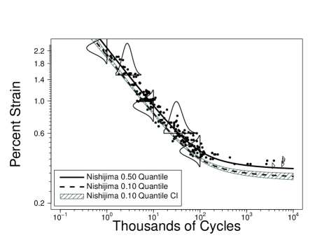
Figure 3: Plot comparing the Nishijima and Coffin–Manson Zero-Elastic-Slope relationships (estimates of the 0.50 quantiles) using a lognormal distribution strength distribution with a constant $\sigma_{X}$ shape parameter for the Inconel 718 fatigue data (a); Plot showing the ML estimates of the 0.10 and 0.50 quantiles and 90% likelihood-based confidence intervals for the 0.10 quantile of the Nishijima/lognormal model (b).

Figure 3b shows ML estimates of the 0.10 and 0.50 quantiles and the band of pointwise 90% likelihood-based confidence intervals for the 0.10 quantile of the Nishijima/lognormal model. The confidence intervals are narrow because of the large amount of data.

Figure 4 illustrates, using the Coffin–Manson model as an example, what happens when fitting an over-parameterized model where the full model is approaching one of the limiting models described in Sections 3.5, 4.6, and 5.6. As mentioned in Section 2.1 such plots provide useful diagnostics if warnings about numerical problems are encountered in ML estimation.

Figure 4a is a two-dimensional relative likelihood profile plot of the $\textrm{qlogis}p$ and $\log\!S_{\textrm{Low}}$ USPs showing a ridge along values of $\textrm{qlogis}p$ less than about $-10$. Figure 4a is a relative likelihood profile plot that focuses on $\textrm{qlogis}p$. This kind of flatness in the likelihood surface will often generate warning messages when maximizing the log-likelihood or inverting the local estimate of the information matrix (used for computing standard errors). The remedy is to use the limiting Coffin–Manson Zero-Elastic-Slope model or equivalently, fix $\textrm{qlogis}p$ at a particular value along the ridge.

(a)	(b)

Figure 4: For the Coffin–Manson model fit to the Inconel 718 data, a two-dimensional profile relative likelihood plot of $\textrm{qlogis}p$ and $\log\!S_{\textrm{Low}}$ (a) and a relative likelihood profile plot of $\textrm{qlogis}p$ (b).

7.2 ML estimation for the Polynt composite material fatigue data

Tridello et al. (2022) and Conte (2022) describe a fatigue test on Polynt SMC LP 2512 R33, a sheet molding compound composite material. Dog-bone-shaped specimens were fabricated and tested in tension-compression fatigue tests at a stress ratio $R=0.10$. Units that survived $10^{6}$ cycles were runouts. The first 15 specimens were tested using a staircase test (a sequential approach that tends to result in stress levels near the center of the fatigue-strength distribution for a specified number of cycles). Subsequently, 20 additional specimens were tested at higher levels of stress to provide more information for estimating the S-N curve. The test resulted in 22 fractured units and 9 runouts. To protect proprietary information, the actual stress values were scaled to have a maximum of 1.

Table 4 gives a summary of estimation results for the Polynt SMC data showing the ten models with the smallest values of AIC.

Table 4: Comparison, for the Polynt SMC data, of the models with the smallest values of AIC

	Model
Model Specified for	Relationship	Distribution	#Parms	$-{\cal L}$	AIC
Fatigue Strength	Rectangular Hyperbola	Weibull	$4$	$-45.8$	$-83.7$
Fatigue Strength	Coffin–Manson Zero Elastic Slope	Weibull	$4$	$-45.8$	$-83.5$
Fatigue Life	Basquin (Inverse Power)	Weibull	$3$	$-44.5$	$-83.0$
Fatigue Life	Box–Cox/Loglinear Sigma	Weibull	$5$	$-46.1$	$-82.3$
Fatigue Strength	Coffin–Manson	Weibull	$5$	$-45.8$	$-81.7$
Fatigue Strength	Nishijima	Weibull	$5$	$-45.8$	$-81.7$
Fatigue Strength	Rectangular Hyperbola	Lognormal	$4$	$-44.8$	$-81.6$
Fatigue Life	Box–Cox/Loglinear Sigma	Lognormal	$5$	$-45.7$	$-81.4$
Fatigue Strength	Coffin–Manson Zero Elastic Slope	Lognormal	$4$	$-44.7$	$-81.3$
Fatigue Strength	Rectangular Hyperbola	Loglogistic	$4$	$-44.5$	$-80.9$

The best fitting models are the Rectangular-Hyperbola/Weibull model (limiting model for the Nishijima/Weibull model, as described in Section 5.6) and the Coffin–Manson Zero Elastic-Slope/Weibull model (limiting model for the Coffin–Manson/Weibull model, as described in Section 4.6). The AIC values for these top two models are close to each other and the two fitted median quantile lines (not shown here), are visually, identical.

Interestingly, the Basquin/Weibull model (linear on log-log scales) also has a small AIC. AIC is less able (compared with the Inconel 718 example) to discriminate among the different Polynt SMC models because there is substantially less information in the data (only 22 fractured units and 9 runouts when compared to 242 fractured units and 4 runouts for the Inconel 718 example). Table 5 gives ML estimates of the TPNSs and corresponding 95% confidence intervals for the Rectangular Hyperbola/Weibull fatigue-strength model.

Table 5: ML estimates and Wald confidence intervals for the TPNS of the Rectangular Hyperbola/Weibull fatigue-strength model fit to the Polynt SMC fatigue data

			95% Confidence Interval
Parameter	Estimate	Std Error	Lower	Upper
$B$	$-9.48$	8.03	$-25.21$	6.26
$C$	14.2	17.27	$-19.66$	$48.05$
$E$	$-1.49$	0.65	$-2.76$	$-0.22$
$\sigma_{X}$	0.091	0.018	0.057	0.126

Figure 5a compares the Rectangular Hyperbola/Weibull and the Basquin/Weibull models.

(a)	(b)

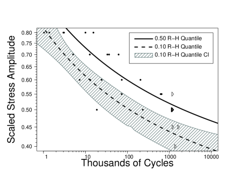
Figure 5: For the Polynt SMC fatigue data, a plot comparing the Rectangular Hyperbola and Basquin Relationships (estimates of the 0.50 quantiles) using a Weibull distribution strength distribution with a constant $\sigma_{X}$ shape parameter (a); Plot showing the ML estimates of the 0.10 and 0.50 quantiles and the band of pointwise 90% likelihood-based confidence intervals for the 0.10 quantile of the Rectangular Hyperbola/Weibull model (b).

The Basquin/Weibull model has a smaller likelihood and a larger AIC (in Table 4) because of lack of fit implied by the substantial number of runouts at the lower levels of stress. Although the Basquin/Weibull is statistically consistent with the limited data, engineering/physical knowledge about the general nature of fatigue-life processes would suggest the Rectangular Hyperbola or the Coffin–Manson Zero Elastic-Slope/Weibull models better choices.

Figure 5b shows, for the Rectangular Hyperbola/Weibull model, the ML estimates of the 0.10 and 0.50 quantiles and the band of pointwise 90% likelihood-based confidence intervals for the 0.10 quantile. The relative width of the confidence bands is considerably wider than in the Inconel 718 example because there is less information in the limited Polynt SMC data.

Next we investigate some potential numerical difficulties that can arise when overfitting a nonlinear regression model and tools to diagnose such difficulties. Two possible difficulties are

• Regions in the parameter space where the likelihood surface is flat or approximately flat.

• A likelihood surface that has more than one maximum, often a global maximum and one or more local maxima.

The flat spots in the likelihood surface can cause warning or error messages from both the optimization algorithm (used to maximize the likelihood) and differentiation algorithms (used to compute the Hessian matrix). When there is more than one maximum in the likelihood surface, as mentioned in Section 2.1, it is possible that the optimization algorithm will converge to a local instead of the global optimum. As mentioned in Section 2.1, we have found that one- and two-dimensional relative likelihood profiles are useful for exploring and finding remedies for these difficulties.

Figure 6a is the profile relative likelihood plot of $\textrm{qlogis}p$ that arises when fitting the Nishijima/Weibull model to the Polynt SMC fatigue data.

(a)	(b)

Figure 6: For the Polynt SMC fatigue data and the Nishijima/Weibull model, profile relative likelihood plot of $\textrm{qlogis}p$ (a) and a plot of the data with the two fitted models corresponding to the two flat parts of the profile relative likelihood plot (b).

The two intervals of $\textrm{qlogis}p$ values where this profile plot is flat suggests two competing descriptions (models) for the data. Over the interval from about $5$ to about $28$ the model fit corresponds to the limiting Rectangular-Hyperbola/Weibull model described in Section 5.6 and illustrated by the dashed fitted line in Figure 6b. Over the interval from $-\infty$ to about $-20$ the model fit corresponds to the limiting Piecewise-Linear/Weibull model also described in Section 5.6 and illustrated by the solid fitted line in Figure 6b. The flatness in these two regions of the profile relative likelihood indicates that there are multiple combinations of the parameter values that result in the same fitted curve. The higher level of the profile relative likelihood for the Piecewise-Linear/Weibull model suggests a somewhat better fit, but both limiting models are consistent with the data. As a practical matter, one could choose the model that provides more conservative inferences. When $\textrm{qlogis}p\rightarrow\infty$, the Nishijima model approaches rectangular hyperbola model. Numerical problems arise for $\textrm{qlogis}p>20$ but the profile would remain horizontally flat if the computations could be done using unlimited precision.

7.3 Summary of the analyses of the benchmark collection of fatigue-life data sets

As mentioned in Section 2.1, it is useful to test newly developed estimation algorithms on a collection benchmark data sets. For the particular applications used in this paper, we used a benchmark collection of 29 fatigue S-N data sets having different shapes and sizes. The data sets were obtained from the statistical and engineering literature and other sources and are available in the online supplementary materials. One of the data sets was simulated precisely to provide a stress test for models that would be over parameterized.

These data sets were used to exercise our computational and statistical algorithms and to provide experience and insights into analytical properties of the nonlinear relationships and limiting cases for the main models described in Sections 4–6 and to fine-tune our definitions of the USPs. In particular, for each of the 29 data sets, the

1. Basquin (Inverse Power)

2. Box–Cox/Loglinear Sigma

3. Coffin–Manson

4. Coffin–Manson Zero Elastic Slope

5. Nishijima

6. Rectangular Hyperbola

S-N relationships were paired with the Fréchet, Loglogistic, Lognormal, and Weibull log-location-scale distributions, for a total of 696 fitted models. The results are summarized in Table 6 which gives, for each data set, the combination of relationship and distribution (i.e., the model) with the smallest AIC.

Table 6: Model with the smallest AIC value for each of the data sets in the benchmark collection

Data Set Name	Model Specified for	Relationship	Distribution	#Parms	$-{\cal L}$	AIC
Aluminum2024-T4	Fatigue Strength	Nishijima	Weibull	$5$	$-1007.1$	$-2004.2$
Aluminum6061-T6	Fatigue Life	Box–Cox/Loglinear Sigma	Loglogistic	$5$	$-567.7$	$-1125.5$
Aluminum6061-T6Censored	Fatigue Life	Box–Cox/Loglinear Sigma	Loglogistic	$5$	$-485.2$	$-960.4$
AnnealedAluminumWire	Fatigue Life	Box–Cox/Loglinear Sigma	Weibull	$5$	$-626.9$	$-1243.7$
AnnealedCopperWire	Fatigue Life	Box–Cox/Loglinear Sigma	Loglogistic	$5$	$-578.3$	$-1146.5$
AnnealedIronWire	Fatigue Strength	Nishijima	Loglogistic	$5$	$-655.7$	$-1301.3$
Basquin.sim30	Fatigue Life	Basquin (Inverse Power)	Lognormal	$3$	$-40.8$	$-75.5$
BKfatigue02	Fatigue Strength	Nishijima	Weibull	$5$	$-167.9$	$-325.8$
C35Steel	Fatigue Strength	Coffin–Manson Zero Elastic Slope	Lognormal	$4$	$-772.0$	$-1536.1$
CeramicBearing02	Fatigue Life	Basquin (Inverse Power)	Weibull	$3$	$-90.5$	$-174.9$
Concrete	Fatigue Strength	Nishijima	Lognormal	$5$	$-514.4$	$-1018.8$
Concrete2	Fatigue Strength	Nishijima	Lognormal	$5$	$-361.8$	$-713.6$
GAS7C3-5GM-TA	Fatigue Strength	Coffin–Manson Zero Elastic Slope	Loglogistic	$4$	$-88.5$	$-169.1$
Inconel718	Fatigue Strength	Nishijima	Lognormal	$5$	$-1276.6$	$-2543.2$
Inconel718LowStrain	Fatigue Strength	Nishijima	Loglogistic	$5$	$-399.8$	$-789.6$
LaminatePanel	Fatigue Strength	Rectangular Hyperbola	Lognormal	$4$	$-259.2$	$-510.3$
MagnesiumAlloyAZ61	Fatigue Life	Box–Cox/Loglinear Sigma	Weibull	$5$	$-78.8$	$-147.5$
NickelWire	Fatigue Strength	Nishijima	Weibull	$5$	$-739.8$	$-1469.5$
Nitinol02	Fatigue Strength	Coffin–Manson	Lognormal	$5$	$-379.9$	$-749.8$
Nitinol03	Fatigue Strength	Coffin–Manson	Lognormal	$5$	$-497.2$	$-984.3$
PolyintSMC	Fatigue Strength	Rectangular Hyperbola	Weibull	$4$	$-45.8$	$-83.7$
SteelCruciformShaped	Fatigue Life	Box–Cox/Loglinear Sigma	Lognormal	$5$	$-80.1$	$-150.2$
SteelS355J2	Fatigue Strength	Coffin–Manson Zero Elastic Slope	Lognormal	$4$	$-171.2$	$-334.3$
SteelWire	Fatigue Strength	Nishijima	Loglogistic	$5$	$-456.1$	$-902.3$
SuperAlloy	Fatigue Strength	Coffin–Manson	Weibull	$5$	$-24.8$	$-39.5$
TBC600Y980T	Fatigue Strength	Coffin–Manson Zero Elastic Slope	Lognormal	$4$	$-32.1$	$-56.2$
Ti64-350F-Rm1Corrected	Fatigue Strength	Rectangular Hyperbola	Lognormal	$4$	$-210.1$	$-412.2$
Titanium02	Fatigue Life	Box–Cox/Loglinear Sigma	Frechet	$5$	$-202.4$	$-394.8$
Triax	Fatigue Strength	Nishijima	Frechet	$5$	$-201.6$	$-393.3$
UltraCleanSteel	Fatigue Strength	Rectangular Hyperbola	Lognormal	$4$	$-25.4$	$-42.7$

For many of the data sets, several models had values of AIC that were very close to the the value for the model with the smallest AIC. In these cases, these fitted models agree well with the best model within the range of the data. In some cases there was an indication of possible convergence failure. For example, in some cases the profile likelihood for a parameter will be approximately flat at a level that is well above 0 (but less than one) as the parameter value approaches $-\infty$ or $\infty$, indicating that the fitted model is not far from one of the limiting models. These occurrences were often for data sets where a limiting model has a higher AIC because the data does not contain enough information to estimate, adequately, all of the parameters of the full model.

8 Concluding Remarks and Areas for Future Research

Nonlinear regression presents challenges for users. Especially when the same group of models will be used frequently for analyses with many different data sets, it is useful to study the analytical properties of the models and design appropriate robust numerical methods for those models. Based on our experiences we have outlined a general procedure for doing this and have provided the details for three of the recent models for which we have developed such algorithms. The ideas here readily extend to applications with more than one explanatory variable and to hierarchical models although there are likely to be some challenges in working out the details.

9 Acknowledgments

Luis A. Escobar provided helpful comments on an earlier version of this paper. Professor Andrea Tridello provided a copy of the Polynt SMC data that we used as an example in Section 7.2.

References

- Barton (1992) Barton, R. R. (1992). Computing forward difference derivatives in engineering optimization. Engineering Optimization 20, 205–224.
- Basquin (1910) Basquin, O. H. (1910). The exponential law of endurance tests. In Proceedings of the American Society for Testing and Materials, Volume 10, pp. 625–630.
- Bates and Watts (1988) Bates, D. and D. G. Watts (1988). Nonlinear Regression Analysis and its Applications. John Wiley & Sons, Inc.
- Berger and Bernardo (1992) Berger, J. O. and J. M. Bernardo (1992). On the development of the reference prior method. Bayesian Statistics 4, 35–60.
- Castillo and Fernández-Canteli (2009) Castillo, E. and A. Fernández-Canteli (2009). A Unified Statistical Methodology for Modeling Fatigue Damage. Springer.
- Conte (2022) Conte, E. (2022). Optimization and implementation of a software code for the automated analysis of fatigue data. Ph. D. thesis, Politecnico di Torino.
- Dowling et al. (2020) Dowling, N. E., S. L. Kampe, and M. V. Kral (2020). Mechanical Behavior of Materials: Engineering Methods for Deformation, Fracture, and Fatigue (Fifth ed.). Pearson.
- Falk (2019) Falk, W. (2019). A statistically rigorous fatigue strength analysis approach applied to medical devices. In Fourth Symposium on Fatigue and Fracture of Metallic Medical Materials and Devices. ASTM International.
- Gabry and Goodrich (2020) Gabry, J. and B. Goodrich (2020). Prior distributions for rstanarm models. URL: https://cran.r-project.org/web/packages/rstanarm/vignettes/priors.html.
- Gallant (1987) Gallant, A. R. (1987). Nonlinear Statistical Models. John Wiley & Sons.
- Huet et al. (2004) Huet, S., A. Bouvier, M.-A. Poursat, and E. Jolivet (2004). Statistical Tools for Nonlinear Regression: A Practical Guide with S-PLUS and R Examples (Second ed.). Springer.
- Meeker et al. (2022) Meeker, W. Q., L. A. Escobar, and F. G. Pascual (2022). Statistical Methods for Reliability Data (Second ed.). Wiley.
- Meeker et al. (2024) Meeker, W. Q., L. A. Escobar, F. G. Pascual, Y. Hong, P. Liu, W. M. Falk, and B. Ananthasayanam (2024). Modern statistical models and methods for estimating fatigue-life and fatigue-strength distributions from experimental data. https://arxiv.org/abs/2212.04550v1. Accessed: 18 March 2024.
- Meeker et al. (2003) Meeker, W. Q., L. A. Escobar, and S. Zayac (2003). Use of sensitivity analysis to assess the effect of model uncertainty in analyzing accelerated life test data. In W. R. Blischke and D. N. P. Murthy (Eds.), Case Studies in Reliability and Maintenance, Chapter 12, pp. 269–292. Wiley.
- Nash (2014) Nash, J. C. (2014). Nonlinear Parameter Optimization Using R Tools. John Wiley & Sons.
- Nelson (1984) Nelson, W. B. (1984). Fitting of fatigue curves with nonconstant standard deviation to data with runouts. Journal of Testing and Evaluation 12, 69–77.
- Ratkowsky (1983) Ratkowsky, D. (1983). Nonlinear Regression Modelling. Marcel Dekker.
- Ross (1970) Ross, G. J. S. (1970). The efficient use of function minimization in non-linear maximum-likelihood estimation. Journal of the Royal Statistical Society: Series C (Applied Statistics) 19, 205–221.
- Ross (1990) Ross, G. J. S. (1990). Nonlinear Estimation. Springer-Verlag.
- Seber and Wild (1989) Seber, G. A. F. and C. J. Wild (1989). Nonlinear Regression. Wiley.
- Shen (1994) Shen, C.-L. (1994). The Statistical Analysis of Fatigue Data. Ph. D. thesis, The University of Arizona.
- Tian et al. (2024) Tian, Q., C. Lewis-Beck, J. B. Niemi, and W. Q. Meeker (2024). Specifying prior distributions in reliability applications (with discussion). Applied Stochastic Models in Business and Industry 44, 5–62.
- Tridello et al. (2022) Tridello, A., C. B. Niutta, F. Berto, M. Tedesco, S. Plano, D. Gabellone, and D. Paolino (2022). Design against fatigue failures: Lower bound PSN curves estimation and influence of runout data. International Journal of Fatigue 162, 106934.