Small Scale Reflection for the Working Lean User

Abstract

We present the design and implementation of the Small Scale Reflection proof methodology and tactic language (a.k.a. SSR) for the Lean 4 proof assistant. Like its Coq predecessor Space Sci. Rev., our Lean 4 implementation, dubbed LeanSSR, provides powerful rewriting principles and means for effective management of hypotheses in the proof context. Unlike Space Sci. Rev.for Coq, LeanSSR does not require explicit switching between the logical and symbolic representation of a goal, allowing for even more concise proof scripts that seamlessly combine deduction steps with proofs by computation.

In this paper, we first provide a gentle introduction to the principles of structuring mechanised proofs using LeanSSR. Next, we show how the native support for metaprogramming in Lean 4 makes it possible to develop LeanSSR entirely within the proof assistant, greatly improving the overall experience of both tactic implementers and proof engineers. Finally, we demonstrate the utility of LeanSSR by conducting two case studies: (a) porting a collection of Coq lemmas about sequences from the widely used Mathematical Components library and (b) reimplementing proofs in the finite set library of Lean’s mathlib4. Both case studies show significant reduction in proof sizes.

1 Introduction

Small Scale Reflection (SSR) is a methodology for structuring deductive machine-assisted proofs that promotes the pervasive use of computable symbolic representations of data properties, in addition to their more conventional logical definitions in the form of inductive relations. Small scale reflection emerged from the prominent effort to mechanise the proof of the Four Colour Theorem in the Coq proof assistant [9], in which the large number of cases to be discharged posed a significant scalability challenge for a traditional proof style based on tactics that operate directly with the logical representation of a goal. Support for small scale reflection in Coq has later been implemented in the form of the Space Sci. Rev.plugin, which provides a concise tactic language, and its associated library of lemmas [11], becoming an indispensable tool for the working Coq user. Space Sci. Rev.has been employed in many projects, including mechanisations of the foundations of group theory [10], measure theory [2], information theory [3], 3D geometry [1], programming language semantics [WeirichVAE17], as well as proving the correctness of heap-manipulating, concurrent and distributed programs [Nanevski-al:POPL10, SergeyNB15, SergeyWT18, PirleaS18], and probabilistic data structures [12]. Two Space Sci. Rev.tutorials [Maboubi-Tassi:MathComp, Sergey:PnP] are currently recommended amongst the basic learning materials for Coq [6].

Lean 4 is a relatively new proof assistant and dependently typed programming language [7]. Like Coq, Lean is based on the Calculus of Constructions with inductive types and is geared towards interactive proofs, coming with extensive support for metaprogramming aimed at simplifying custom proof automation and code generation. Unlike Coq, Lean assumes axioms of classical logic, such as the law of excluded middle. Very much in the spirit of the SSR philosophy of reflecting proofs about decidable propositions into Boolean-returning computations, Lean encourages the use of such propositions (implemented as an instance of the Decidable type class) as if they were Boolean expressions, going as far as providing a program-level if-then-else operator that performs conditioning on an instance of a decidable proposition. Given this similarity of approaches, it was only natural for us to try to bring the familiar SSR tactic language to Lean, as an alternative to Lean’s descriptive but verbose idiomatic approach to proof construction. Our secondary motivation was to put Lean’s metaprogramming to the test, implementing SSR entirely within the proof assistant, in contrast with Space Sci. Rev., which is implemented as a Coq plugin in OCaml.

In this paper, we present LeanSSR, a proof scripting language that faithfully replicates the Space Sci. Rev.experience in Lean, yet provides substantially better proof ergonomics, thanks to Lean’s distinctive features, improving on its Coq predecessor in the following three aspects:

1. Usability: Compared to Coq/Space Sci. Rev., which only shows the proof context between complete series of chained tactic applications, LeanSSR provides a more fine-grained access to the proof state, displaying its changes after executing each “atomic” step—a feature made possible by Lean’s mechanism of proof state annotations.

2. Expressivity: Unlike Space Sci. Rev.for Coq, LeanSSR does not require the user to explicitly switch between representation of facts as logical propositions or as symbolic expressions to advance the proof. In particular, this automation makes it possible to unify simplifications via computation and via equality-based rewriting, resulting in very concise proof scripts.

3. Extensibility: Since LeanSSR is lightweight, i.e., it is implemented entirely in Lean using its metaprogramming facilities, it can be easily enhanced with additional tactics and proof automation machineries specific to a particular project that uses it.

In the rest of the paper, we showcase LeanSSR, substantiating the three claims above.

Contributions and Outline.  In this work, we make the following contributions:

• An implementation of LeanSSR, an Space Sci. Rev.-style tactic language for Lean.

• A tutorial on using LeanSSR following a series of characteristic proof examples (Sec. 2).

• A detailed overview of Lean metaprogramming features that we consider essential for implementing LeanSSR and the effect of those features on the end-user experience (Sec. 3).

• Two case studies demonstrating LeanSSR’s utility for proof migration and evolution: (a) porting a collection of Coq lemmas about finite sequences from the MathComp library [Maboubi-Tassi:MathComp] to Lean and (b) reimplementing proofs from the finite set library of Lean’s mathlib4 in LeanSSR (Sec. 4). While proof sizes reduce in both cases, we also comment on our overall better mechanisation experience, compared to refactoring original proofs in both Coq and Lean—thanks to the improved usability aspect highlighted above.

2 LeanSSR in Action

In this section we give a tutorial on the main elements of the LeanSSR proof language. We do not expect the reader to be familiar with the standard Lean tactics. This section will also be informative for the readers familiar with Space Sci. Rev.for Coq due to the improvements LeanSSR makes over Space Sci. Rev.in terms of usability (LABEL:sec:debug) and expressivity (LABEL:sec:refl).

2.1 Managing the Context and the Goal in Backward Proofs

As customary for interactive proof assistants based on higher-order logic, Lean represents the proof state as a logical sequent, as depicted in Fig. 1.

[] c_i : T_i …F_k : P_k … ∀x_l : T_l,  …, P_n →…→C

Fig. 1: Proof state as a sequent

The proof goal is the logical statement below the horizontal line; above the line is the local context of the sequent, a set of constants $c_{i}$ and facts (i.e., hypotheses) $F_{k}$. The goal statement itself can be decomposed into (a) goal context: quantified variables $x_{l}:T_{l}$ and assumptions $P_{n}$, and (b) the conclusion statement $C$. Both local and goal contexts capture the bound variables (term-level or hypotheses) of the overall proof term to be constructed, with the only difference being the explicit names of the variables in the local context. Lean tactics, such as apply, operate directly on the goal’s conclusion using variables from the local context referring to them by their names, while tactics such as intro and revert move variables/hypotheses between the local and the goal context. In practice, such “bookkeeping” of variables and hypotheses contributes most of the proof script burden; so, following Space Sci. Rev., LeanSSR provides tactics to streamline it.

Specifically, LeanSSR provides mechanisms to operate directly with the goal context, treating the goal as a stack, where the left-most variable or assumption is the top of the stack, and the conclusion is always at the bottom of the stack. By convention, most of LeanSSR tactics, operate with the top element of the goal stack. As an example, LeanSSR defines sapply, a variant of the standard Lean apply tactics (many LeanSSR tactics come with the prefix s* to distinguish them from their standard Lean counterparts) to simplify backward proofs [4, Chapter 3]. As 2(a) shows, sapply applies the first element on the goal stack (i.e., the hypothesis of type $\alpha$) to the rest of the stack (i.e., the goal’s conclusion $\alpha$).

⬇

example: α -> α :=

by sapply

(a) Using sapply tactic

⬇

example: @a -> @b -> @a :=

by move=> hA ?

move: hA; sapply\end{lstlisting}

\caption{Basic \lssr proof script}

\label{fig:inro-rev1}

\end{subfigure}

\begin{subfigure}{0.40\textwidth}

\begin{lstlisting}

example: @a -> (@a -> @b) -> @b :=

by move=> /[swap] hAiB

sapply: hAiB\end{lstlisting}

% \begin{lstlisting}

% example : ∀ x y : α, P x y ->

% ¬ ¬ P x y := by

% move=> > hPxy hNPxy

% sby apply hNPxy

% \end{lstlisting}

% \vspace{-4mm}

\caption{A proof using \fcode{/[swap]} intro pattern}

\label{fig:inro-rev2}

\end{subfigure}

\caption{\lssr proof scripts using the \fcode{sapply} tactic,

\code{=>} and \code{:} tacticals, and intro patterns.}

\label{fig:inro-rev}

\end{figure}

%

A typical proof in \lssr is done by moving variables and assumptions

back and forth between the local context and the goal context, placing

the terms to be used in a current proof step on top of the goal

stack.

%

Such proof context management is done via two complementary

\emph{tacticals}: \code{=>} and \code{:}.

%

The former one (\code{=>}) moves facts above the sequent line, whereas

the latter one moves facts below, “pushing” them to the goal stack.

%

\autoref{fig:inro-rev1} and~\ref{fig:inro-rev2} showcase the usage of

\code{=>} and \code{:}.

%

The proof in \autoref{fig:inro-rev1} starts with \code{move=> hA ?},

where \code{move} essentially does nothing: its goal is to serve as a no-op

tactic, to be followed by either \code{=>} or~\code{:}.

%

What follows (\code{ => hA ?}) is an example of an \emph{intro

pattern} (more patterns will be shown below) that introduces the first

two elements of the goal context, the first named \code{hA} and the

second with an auto-generated name.

%

To apply the introduced assumption \code{hA} we have to revert it back

to the top of the proof context; the next line \code{move: hA} does

exactly that.

Lean users might notice that \code{=>} and \code{:} are similar to the

standard \code{intro} and \code{revert} Lean tactics.

%

\autoref{fig:inro-rev2} demonstrates the versatility of the \lssr

tacticals when combined with different intro patterns.

%

% First, \code{=>} provides better support for moving facts

% \emph{within} a goal context.

%

For instance, to swap the first two elements of the proof stack,

\autoref{fig:inro-rev2} makes use of the \code{/[swap]} intro pattern.

%

This will turn our goal to \code{(@a -> @b) -> @a -> @b}.

%

Other useful \ssr-inspired intro patterns include \code{*} for

introducing \emph{all} elements on the proof stack, \texttt{_} for

discarding the first element on the proof stack, and \code{/[dup]} for

duplicating the first element on the stack.

%

Furthermore, as the purpose of \lssr tacticals is to “massage” the

shape of the goal, they can be smoothly combined with other \lssr

tactics that operate directly on the goal stack.

%

In particular, \autoref{fig:inro-rev2} combines \code{sapply}

with~\code{:} (\ie, \code{sapply: hAiB}), with the effect of first

pushing \code{hAiB : @a -> @b} to the goal stack and then executing

the \code{sapply} tactic, discharging the goal similarly to the example

from \autoref{fig:sapply}.

\subsection{Induction, Case Analysis, and Last-Mile Automation}

\begin{wrapfigure}[7]{r}{0.46\textwidth}

\vspace{-8pt}

\captionsetup{aboveskip=5pt}

\begin{lstlisting}

example (m n : Nat): n <= m ->

m - n + n = m := by

elim: n m=> [| n IHn [| m’]] //==

move=> ?; srw -[2](IHn m’) //\end{lstlisting}

\caption{A proof by mathematical induction}

\label{fig:elim}

\end{wrapfigure}

\noindent

%

\lssr combines the tacticals for the goal context management and intro

patterns with tactics for proofs by induction and case analysis.

%

In particular, \lssr introduces a variant of a standard

\code{induction} tactic called \code{elim}, which expects no explicit

arguments and simply applies the induction principle of

the top element of the goal stack.

%

As an example, consider the proof by induction in \autoref{fig:elim}

of a simple property of natural addition and subtraction.

%

As its first step, the proof generalises the two natural constants,

\code{n} and~\code{m} by pushing them onto the goal, making it

\code{@all n m, n <= m -> m - n + n = m};

%

it is followed by an invocation of the induction principle for natural

numbers on \code{n}, with \code{m} being universally quantified; all

that expressed simply as \code{elim: n m}.

Unlike Lean’s \code{induction} tactic, \code{elim} does not introduce

new variables and facts to the local context, leaving those

universally quantified in the respective subgoals.

%

In our example, using \code{elim} on a natural number introduces two

subgoals, one for the base \code{zero} and one for the inductive step

\code{succ}, with the latter featuring a predecessor variable and an

inductive hypothesis.

%

Naming variables in subgoals can be done using the \emph{alternation

separator} intro pattern of the form \text{[ … | … | … ]}

where each \texttt{…} section corresponds to introductions in a

respective subgoal.

%

We can, thus, revise our proof to be \code{elim: n m=>[| n IHn]},

introducing the variable and the hypothesis step to the local context

as \code{n} and \code{IHn}, respectively.

Let us focus on the second subgoal (\ie, the inductive step), which

now looks as follows:

%

\vspace{-3pt}

%

\begin{equation}

\forall m,\, n + 1 \leq m \to m - (n + 1) + (n + 1) = m

\label{eq:goal}

\end{equation}

%

%\vspace{-3pt}

%

The proof of \eqref{eq:goal} can be finished by the case analysis

on~\code{m} using \lssr’s \code{scase} tactic, which will generate two

subgoals, one for \code{zero} and one for~\code{succ}. The latter will

introduce yet another universally-quantified variable, which can be

suitably named and moved to the local context: \code{scase=> [| m’]}.

%

Such nested deconstructions of a goal’s top variable into cases are so

frequent that \lssr overloads the alternation separator intro pattern

to perform case analyses with simultaneous naming. Hence, we can now

revise our proof to first perform top-level induction on~\code{n} and

then do case analysis on~\code{m} in the resulting second subgoal via

\code{elim: n m=> [| n IHn [| m’]]}.

Having executed this proof script line, we are left with three

subgoals to discharge:

%

% \begin{gather}

\begin{align}

\forall m : \mathbb{N},\, 0 \leq m &\to m - 0 + 0 = m \label{eq:goal2}

\\

n + 1 \leq 0 &\to 0 - (n + 1) + (n + 1) = 0 \label{eq:goal3}

\\

(n + 1) \leq (m + 1) &\to (m + 1) - (n + 1) + (n + 1) = (m + 1) \label{eq:goal4}

\end{align}

%

This would be a good time to make use of Lean’s famous automation to

solve~\eqref{eq:goal2} and \eqref{eq:goal3}, and simplify

\eqref{eq:goal4}.

%

\lssr provides the following intro patterns for such “last-mile”

automation:

%

\begin{itemize}

\item \code{/=} for simplification by evaluation (Lean’s \code{dsimp})

and \code{/==} for proofs by rewriting (\code{simp})

\item \code{//} for a lightweight automation combining Lean tactics

\code{trivial} and \code{simp_all}

\item \code{//=} abbreviating \code{dsimp=> //}, and \code{//==}

abbreviating \code{simp=> //}

\end{itemize}

%

In this case, using \code{//==} on all generated subgoals leaves us

with only one obligation to prove:

%

\vspace{-10pt}

%

\begin{equation}\label{eq:goal5}

n \leq m’ \to m’ - n + (n + 1) = (\gbm{m’} + 1)

\end{equation}

%

\vspace{-10pt}

%

\subsection{Targeted Rewriting using Equality Hypotheses}

\noindent

%

The remaining goal~\eqref{eq:goal5} can be proven using the previously

introduced induction hypothesis \code{IHn : @all (m : Nat), n ≤ m → m

- n + n = m}.

%

Intuitively, the proof can be completed by replacing the

\graybox{highlighted} \emph{second} occurrence of $m’$ in

\eqref{eq:goal5} with $m’ - n + n$ using the right-hand side of the

equality in \code{IHn}, and then finish the proof by the properties of

linear arithmetic and reflexivity.

%

This can be achieved by \lssr rewriting tactic \code{srw} allowing one

to specify the term occurrence to be rewritten.

%

The proof script in \autoref{fig:elim} ends with moving the inequality

\code{n ≤ m’} to the local context via \code{move=>?}, followed by

\code{srw -[2](IHn m’) //}, where \code{-} stands for the

right-to-left rewrite direction and \code{[2]} denotes the specific

occurrence of \code{m’}.

%

Performing this rewrite generates the obligation \code{n ≤ m’}, which

is discharged via \code{//}.

The \code{srw} tactic generalises Lean’s vanilla \code{rw}, allowing

for constructions such as:

%

\vspace{-3pt}

%

\[

\text{\code{srw (drop_nth _ lt_i_m) //== -[1]h nth_index //

-index_mem}}

\]

%

\vspace{-3pt}

%

that interleave rewrites with simplifications, resolving the appearing

subgoals with~\code{//}.

%

\vspace{-5pt}

\subsection{Fine-Grained Proof State Exploration and Error

Highlighting}

\label{sec:debug}

\noindent

%

As our examples so far demonstrate, proofs in \lssr tend to be quite

compact, thanks to the concise nature of the tactic language that

chains multiple manipulations with the goal and the proof context into

a single line of a proof script.

%

The downside of this style is that proofs often become difficult to

follow and refactor—a frequent complaint by newcomers to

Coq/\ssr who are familiar with the vanilla Coq proof mode.

%

The problem of proof script understanding and maintenance in \ssr is

exacerbated by the fact that Coq can only display the proof context

between \emph{complete} series of chained tactic applications

separated by periods.

%

When a mistake is made in the middle of a line in an \ssr

proof script, one typically has to manually break the line into

period-terminated parts, performing a binary search-style debugging.

%

In addition to that, if a particular intro pattern cannot be applied

in \ssr, say we write \code{[| | m]} with three alternations instead

of two in the proof of \autoref{fig:elim}, Coq will report an error

for the entire script line, further complicating the search for a fix.

% So, if something goes wrong in the middle of \ssr script line, it

% usually hard to break this line down into two parts: before and after

% the break point, executing only the first part, to see what exactly

% went wrong. Moreover, if a particular intro pattern fails, say we

% write \code{[| | m]} with three alternations instead of two, Coq/\ssr

% will highlight in red the whole line, so we won’t even know where

% exactly does the error occur.

\begin{figure}[t]

\begin{subfigure}{0.49\textwidth}

\fbox{\includegraphics[width=0.95\textwidth]{figures/image2.pdf}}

\caption{The proof view before introducig \code{IHn}}

\label{fig:before-IHn}

\end{subfigure}

\begin{subfigure}{0.49\textwidth}

\fbox{\includegraphics[width=0.945\textwidth]{figures/image1.pdf}}

\caption{The proof view after introducig \code{IHn}}

\label{fig:after-IHn}

\end{subfigure}

\captionsetup{aboveskip=5pt}

\captionsetup{belowskip=-10pt}

\caption{Visual support for fine-grained proof state exploration

with \lssr proof scripts.}

\end{figure}

\lssr overcomes these hurdles, providing an improved (compared to

\ssr) experience to the users, thereby substantiating the usability

claim~(\ref{label:ui}) from \autoref{sec:intro}.

First, the better proof debugging is made possible by the powerful

feature of Lean that allows the DSL designer to annotate each symbol

in the tactic definition with the proof state before and after its

execution.

%

For instance, if the user puts the pointer in the text buffer with her

proof script before the \code{IHn} token in \autoref{fig:elim}, the

goal display will be as in \autoref{fig:before-IHn}, highlighting the

upcoming change in the goal in red.

%

For the pointer positioned right after \code{IHn}, the goal display

shows the proof context as in~\autoref{fig:after-IHn}.

%

Second, Lean provides a tunable mechanism for precise error

highlighting, so if we write \code{[| | m]} with three alternations

instead of two, only highlight the \code{[| | m]} part of the script

will be marked as an error.

%

% In our experience, these two features, fine-grained context changes

% and precise error highlighting, drastically reduce the time it takes

% to find errors in \lssr proofs.

% If you change some definition, and

% the whole proof goes wrong, you can easily identify the place where

% does it break, as well as see the proof context around this place.

\vspace{-5pt}

\subsection{Forward Reasoning via Views}

\label{sec:views}

\begin{wrapfigure}[8]{r}{0.46\textwidth}

\vspace{-8pt}

\captionsetup{aboveskip=2pt}

\begin{lstlisting}

example (A B C : Prop) :

(A → B) → (B → C) → A → C :=

by intro AiB BiC Ha

apply BiC

apply AiB

exact Ha\end{lstlisting}

\caption{A backward proof in vanilla Lean}

\label{fig:back}

\end{wrapfigure}

%

\noindent

%

So-called \emph{backward} proofs, in which a conclusion of a goal is

gradually strengthened to be eventually discharged from the available

hypotheses or axioms, are prevalent in interactive proofs.

%

A very simple example of such a proof is given in \autoref{fig:back},

which proves the conclusion~\code{C} using the reverse-order

applications of the assumptions \code{BiC}, \code{AiB}, and,

eventually, \texttt{Ha~:~A}.

\begin{wrapfigure}[8]{r}{0.46\textwidth}

\vspace{-8pt}

\captionsetup{aboveskip=2pt}

\begin{lstlisting}

example (A B C : Prop) :

(A → B) → (B → C) → (A → C) :=

fun AiB BiC Ha ↦

have Hb : B := AiB Ha

have Hc : C := BiC Hb

show C from Hc\end{lstlisting}

\caption{A forward proof in vanilla Lean}

\label{fig:forw}

\end{wrapfigure}

%

That said, proof engineers trained in a tradition of purely

mathematical proofs often prefer the complementary \emph{forward}

style, in which the assumptions are gradually weakened to eventually

imply the conclusion~\cite[Chapter~4]{love}.

%

A typical forward proof in Lean follows the so-called

\emph{assume}/\emph{have}/\emph{show} pattern, which explicitly states

the $\forall$-quantified variables and hypotheses as parameters of the

proof term (\emph{assume}) and the proof is comprises a number of

established auxiliary facts (\emph{have}) that make the derivation of

the conclusion trivial (\emph{show}).

%

An example of such a forward proof in the conventional Lean notation

is shown in \autoref{fig:forw}.

\lssr offers an alternative way to construct forward proofs using the

idea of \emph{view intro patterns} or simply \emph{views}, adopted

from the original \ssr~\cite{Gonthier-al:TR}.

%

The proof of the fact from \autoref{fig:back} and~\ref{fig:forw} can

be achieved in \lssr by the following single line:

%

\vspace{-3pt}

%

\begin{center}

\code{by sby move=> AiB BiC /AiB/BiC}

\end{center}

%

\vspace{-3pt}

%

Ignoring \code{sby} for a moment, notice that the proof first moves

the hypotheses \code{AiB : A → B} and \code{BiC : B → C} to the

context.

%

What follows is an application of \code{AiB} to the leading (\ie, top)

assumption of the goal \code{A}, which “switches” it to \code{B},

making the goal to be \code{B → C}.

%

The subsequent view \code{/BiC} switches the leading assumption from

\code{B} to \code{C}.

%

The remaining goal \code{C → C} can be discharged by \code{trivial}

(or \lssr’s \code{//}).

%

This is done by the \code{sby} tactical at the beginning of the line,

which either completes the proof via \code{//} or fails.

%

In fact, this makes the second view redundant, so the proof can be

shortened to \code{by sby move=> AiB ? /AiB}.

\vspace{-5pt}

\subsection{Proofs by Computational Reflection}

\label{sec:refl}

The \lssr demonstration in \autoref{sec:move}–\ref{sec:views} was

merely a build-up to the true essence of the framework: mechanised

reasoning that features both \emph{deduction} and \emph{proof via

computation} by manipulating with equivalent \emph{logical} and

\emph{symbolic} representations of decidable facts.

\begin{figure}[t]

\begin{tabular}{c}

\begin{subfigure}{0.5\textwidth}

\captionsetup{aboveskip=0pt}

\begin{lstlisting}

inductive even : Nat → Prop

where

| ev0 : even 0

| ev2 : ∀ n, even n → even (n + 2)

(b) Even numbers as a logical predicate

⬇

def evenb : Nat → Bool

| 0 => true

| 1 => false

| n + 2 => evenb n

(c) Even numbers via a Boolean function

⬇

@[reflect] instance evenP n : Reflect (even n) (evenb n) := …

#reflect even evenb

example n m : even n → even (m + n) = even m := by

elim=> // n’ _ <-

srw -Nat.add_assoc /==

(d) A proof using reflection between the logical (even) and symbolic (evenb) definition of even numbers.

Two equivalent definitions of even numbers (top), and a proof by reflection (bottom). As a motivating example showing how to unify both these proof styles in LeanSSR, consider the following simple proposition: assuming $n$ is even, $n+m$ is even if and only if $m$ is even. How should we express a decidable property, such as evenness? Proof assistants based on higher-order logic, such as Coq, Isabelle/HOL, and Lean provide two conceptual ways to do so: as a predicate (cf. 2(b)) and as a function (cf. 2(c)). The former style comes with an advantage of providing a richer knowledge when a property occurs in a goal’s assumption, e.g., by assuming even n we can deduce that it’s either zero or another even number plus two. The latter comes with a set of reduction/rewrite principles, such as, evenb n + 2 = evenb n, which is advantageous for simplifying the conclusion of a goal. One can indeed establish an equivalence between the definitions even and evenb, proving that @all n, even n ↔(evenb n = true). Such an equivalence, when expressed as an instance of the Decidable type class in Lean, can be exploited by allowing the user to define computations that explicitly feature a predicate instead of its computable version, such as:

def even_indicator (n: Nat) : Nat := if even n then 1 else 0

This treatment of decidability also explains the somewhat frivolous phrasing of our proposition of interest in terms equality instead of bi-implication (<->) in the statement in 2(d). To summarise, for Decidable properties, Lean aggressively promotes the logical definitions to be considered as “primary”, while the symbolic ones serving merely as helpers for defining computations and, occasionally, for simplifying goals in the proofs about equivalent predicates. This is exactly where LeanSSR comes into play, making such simplifications transparent to the user. Consider the proof of the example in 2(d). The first line initiates the induction on the even n premise, discharging the first trivial subgoal (for the case ev0), binding the first argument n’ of the case ev2, ignoring the even n’ assumption (via _), and performing the right-to-left rewrite using the induction hypothesis even (m +n’) = even m in the conclusion (via the <- intro pattern), leaving us with the following goal to prove:

even (m + (n’ + 2)) = even (m + n’)

The remaining goal is not difficult to prove by using associativity of addition and showing that @all x, even (x + 2) = even x. But also, this is an equality that we should have “for free”, as it can be derived from the last clause of the definition of evenb in 2(c)! To account for scenarios like this one, LeanSSR provides a machinery that allows one to inherit reduction rules of a recursive (symbolic) boolean definition b to simplify instances of the equivalent logical proposition P. To achieve that, one must prove an instance of the Reflect Pb predicate, which is essentially equivalent to proving P ↔(b = true) (we postpone the details of the Reflect definition until Sec. 3) and register this equivalence using the pragma #reflect P b, which is exactly what is done by the first two lines of 2(d). In this case, doing so will add three simplification rules for even into a database of rewrites used by simplification tactics such as simp and the corresponding LeanSSR patterns, e.g., /==:

even 0 = True   even 1 = False   @all n, even (n + 2) = even n

These equalities allow us to finish the proof by /==, rewriting even as if it were evenb. LeanSSR’s Reflect type class is well integrated with the current Lean ecosystem. Once one has proven Reflect P b, the corresponding Decidable instance is automatically derived for P. Readers familiar with Space Sci. Rev.for Coq could notice that a proof of the statement from 2(d) in it would be more verbose, as it would require an explicit switching between the logical predicate and its symbolic counterpart in the conclusion by applying a special Reflect-lemma to the goal. This is not necessary in LeanSSR thanks to Lean’s ability to use the derived rewriting principles (e.g., the three above for even) directly on logical representations. We believe this example supports the expressivity claim (2) from Sec. 1.

2.2 Putting It All Together

We conclude this tutorial by showing how all the features of LeanSSR introduced in Sec. 2.1–LABEL:sec:refl work in tandem in a proof of an interesting property: transitivity of the subsequence relation on lists of elements with decidable equality. 3(a) presents two ways to define the relation. The first one is via a predicate and an auxiliary mask function. The mask function takes two lists: a list of Boolean values m and a list s of elements of some type @a. For each element of s, mask removes it if an element in m at the same position is either false or not present (i.e., m is shorter than s). Then the representation of subsequence as a logical predicate states that s1 is a subsequence of s2, if mask m s2 = s1 for some mask m. The second definition is via a total recursive function subseqb returning a Boolean. This definition we checks that each element in the first list corresponds to some element in the second list using the decidable equality on the values of type $\alpha$, whose existence is postulated in the first line of the listing. For the propositional and Boolean representations above, we can prove a Reflect instance (cf. LABEL:sec:refl), and transport reduction principles of subseqb to subseq by adding the #reflect pragma as at the line 1 of 3(b).

⬇

variable {α : Type} [DecidableEq α]

def mask: List Bool → List α → List α

| b :: m, x :: s =>

if b then x :: mask m s else mask m s

| _, _ => []

def subseq (s1 s2 : List α) : Prop :=

∃ m, length m = length s2 /\

s1 = mask m s2

def subseqb: List α → List α → Bool

| [], _ :: _ => true

| s, [] => s = []

| s@(x :: s’), y :: r =>

subseqb (if x = y then s’ else s) r

(a) Two representations of the subsequence relation

⬇

1#reflect subseq subseqb

2

3def transitive (R: α → α → Prop) :=

4 ∀x y z, R x y → R y z → R x z

5

6example: transitive (@subseq α) := by

7 move=> ?? s ![m2 _ ->] ![m1 _ ->]

8 elim: s m1 m2=> [// |x s IHs1]

9 scase=> [// | [] m1 /= m2]

10 { -- m1’s head is false

11 scase!: (IHs1 m1 m2)=> m sz_m ->

12 sby exists (false :: m) }

13 -- m1’s head is true

14 scase: m2=> [|[] m2] //=

15 scase!: (IHs1 m1 m2)=> m sz_m ->

16 sby exists (false :: m)

(b) Proof that subseq is transitive

Fig. 3: A subsequence relation and the proof of its transitivity in LeanSSR.

3(b) shows the entire transitivity proof. At line 7, it introduces a new intro pattern ![...], which is an advanced version of the case analysis [...]: not only does it destruct the structure on top of the proof stack, but also does so for its nested structures. For instance, the second occurrence of ![...] will turn the goal (∃m, length m = length s ∧ w = mask m s) → ... into @all m, length m = length s → w = mask m s → ... by destructing both the existential quantifier (i.e., the dependent product) and its nested conjunction. The remaining in-place rewrites (via ->) at the line 7 turn the goal into:

subseq (mask m2 (mask m1 s)) s (1)

In plain text, we have to show that if we apply mask to some sequence s with two arbitrary masks, m1 and m2, the resulting sequences would be a subsequence of s. Line 8 advances the proof by induction on s, after generalising the goal over m1 and m2 and discharging the base case with //, which implicitly uses the rewrites allowed by the definition of mask.Next, line 9 performs the case analysis on m1. When it is empty, goal (1) becomes subseq [] s, which can be automatically reduced to True by employing the reflection between subseq and subseqb. The case when m2 is empty is handled automatically in a similar fashion at line 14. We are now left with the following two remaining goals:

• If m1 is non-empty and its first element is false (lines 11-12), then after all simplifications, goal (1) is reduced to subseq (mask m2 (mask m1 s)) (x :: s), where x is a head of the initial list s. Here we employ the induction hypothesis IHs1 at line 11, to state that mask m2 (mask m1 s) is a subsequence of s, which means that mask m2 (mask m1 s) is just mask m s, for some mask m. To finish the proof we instantiate the existential quantifier in the definition of subseq by taking false :: m, which, when applied to x :: s produces exactly mask m s (line 12).

• If the first element of m1 is true, we perform case analysis on m2 (line 14), dispatching the empty case in a way similar to dealing with m1 at line 9. When m2’s first element is also true is trivial as in this case neither of the masks removes the head of s and our goal will simplify to subseq (x :: maskm2 (mask m1 s)) (x :: s) and then, by reflection, to subseq(mask m2 (mask m1 s)) s, which is trivially implied by the induction hypothesis. All this is done by //= at the end of line 14. Finally, the case when m2’s head is false (lines 15-16) is similar to the proof at lines 11-12.

The proof in Fig. 3 comes from our case study: migrating the MathComp library seq from Coq/Space Sci. Rev.to Lean. In Sec. 4.1 we will further elaborate on this mechanisation effort.

3 Implementing LeanSSR using Lean Metaprogramming

In this section we shed light on the implementation of LeanSSR, which makes extensive use of Lean’s metaprogramming facilities. Despite the abundance of available tutorials on implementing tactics in Lean, it still took significant effort to understand how to compose different features to achieve the desired behaviour, following examples from the Lean Metaprogramming Book [metalean], several research papers [selsam2020tabled, Ullrich2022], Lean source code, and online meetings with Lean developers. This makes us believe that our report on this experience might be of interest even for seasoned Lean users who consider developing their own tactics. Besides the new LeanSSR-specific tactics, such as elim, scase, sapply, etc., the three essential enhancements made by LeanSSR over the vanilla Lean tactic language are:

1. Intro patterns: the set of commands that can follow =>

2. Rewrite patterns: the set of commands that can follow srw

3. Revert patterns: the set of commands that can follow :

We refer to those commands as patterns because they are meant to (partially) match some part of the goal. The first set, i.e., intro patterns, includes ?, *, [..| ... | ..], etc. The second set, rewrite patterns, includes eq, [i j...]eq, -[i j ...]eq, etc, where eq is an arbitrary equality fact. For the sake of space, we do not detail revert patterns in this paper, but they are fully documented in the README file of the accompanying code repository [8]. The characterisation of the three pattern categories is non-exclusive: some LeanSSR commands, e.g., // and /==, can be used both as intro patterns (following =>) and rewrite patterns (following srw). To avoid code duplication, those “last-mile automation” commands themself form a set of automation patterns that are implemented separately and then registered to work in positions of both intro and rewrite patterns.

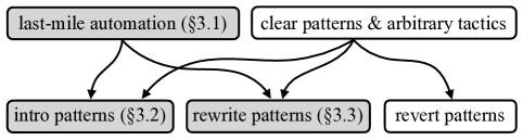
Fig. 4: High-level structure of LeanSSR

An informal depiction of LeanSSR patterns can be found in Fig. 4. Each box stands for a separate set of pattens, the arrows denote the dependencies between those sets. In Sec. 3.1–LABEL:sec:srw, we discuss the implementation of the components highlighted by grey boxes, concluding with a discussion on LeanSSR support for computational reflection in Sec. 3.3. We do not assume the reader to be familiar with metaprogramming in Lean and will explain the required notions as we progress with our presentation.

3.1 Syntax, Macros, and Elaboration for the Last-Mile Automation

We start by discussing the three key features of Lean metaprogramming essential for our LeanSSR embedding: (1) syntactic categories, (2) macro-expansion, and (3) elaboration rules, using the implementation of automation patterns as an example. The implementation is shown in Fig. 5. At the high level, we first define a syntax for a sequence of such patterns (lines 1-8), then tell Lean how to execute such a sequence (lines 10-22), concluding with the definition of sby tactical. More detailed explanation of the code follows below.

⬇

1declare_syntax_cat ssrTriv

2syntax "//" : ssrTriv

3syntax "/=" : ssrTriv

4syntax "/==" : ssrTriv

5syntax "//=" : ssrTriv

6syntax "//==" : ssrTriv

7declare_syntax_cat ssrTrivs

8syntax (ppSpace colGt ssrTriv)* : ssrTrivs

9

10elab_rules : tactic

11 | ‘(ssrTriv| /=) =>

12 run ‘(tactic| try dsimp)

13 | ‘(ssrTriv| /==) =>

14 run ‘(tactic| try simp)

15 | ‘(ssrTriv| //) => ... -- omitted

⬇

16macro_rules

17 | ‘(ssrTriv| //= ) => ‘(ssrTrivs| /= // )

18 | ‘(ssrTriv| //==) => ‘(ssrTrivs| /== //)

19

20elab_rules : tactic

21 | ‘(ssrTrivs| $ts : ssrTriv *) =>

22 for t in ts do allGoals $ evalTactic t

23

24elab sby:"sby " ts : tacticSeq : tactic => do

25 evalTactic ts

26 unless (<- getUnsolvedGoals).length = 0 do

27 allGoals $ run ‘(ssrTriv| //)

28 unless (<- getUnsolvedGoals).length = 0 do

29 throwErrorAt sby "No applicable tactic"

Fig. 5: Implementing of last-mile automation in LeanSSR using Lean metaprogramming.

Line 1 defines a syntactic category called ssrTriv for the LeanSSR automation patterns. One can think of a syntactic category as of a set of syntax expressions grouped together under a single name, for which interpretations can be given. Next, lines 2-6 define elements of this category: //, /=, /==, //= and //==. At line 7, we define yet another syntax category ssrTrivs for sequencing automation patterns. Elements of this category are iterated sequences of ssrTriv separated with a space ppSpace. To ensure that Lean does not try to parse the next line after a sequence of the patterns ssrTriv as a its continuation, we also insert the colGt element, which allows for line breaks, but only if the column number of the pattern on a new line is greater than the column number of the last pattern on the line above, in the spirit of Landin’s Offside Rule [15]. Having defined the syntax for the automation pattern, we proceed to ascribe semantics to it. Lines 10-15 give a meaning to basic automation patterns by using Lean’s standard mechanism of elaboration rules via the elab_rules directive. Each elaboration rule maps a piece of a syntax into an execution inside Lean’s TacticM monad [4, §8.3], thus defining a tactic in terms of other Lean tactics, with access to the global proof state. For example, /= is elaborated into executing the standard try dsimp tactic (lines 11-12). The remaining automation patterns, //= and //== are defined in terms of the more primitive elements of ssrTriv. This is done using Lean’s rules for macro-expansions, following the macro_rules directive. Macro-expansion rules in Lean map elements of syntax into executions within the MacroM monad, returning another element of syntax as a result. Those rules are applied by the Lean interpreter after the parsing stage, but before the elaboration stage. Here, we simply expand //= to /= //, and //== to /== //, as shown at lines 16-18 of Fig. 5. Since both //= and //== are represented as elements of the ssrTrivs category, we have to tell Lean how to elaborate them as well. For the sake of demonstration, we are going to do it by employing one of the most powerful tools in Lean’s metaprogramming toolbox: the evalTactic directive. This directive takes an arbitrary piece of syntax and tries to elaborate it into a sequence of tactics to be executed, using a set of macro-expansion and elaboration rules available in the dynamic context, i.e., the rules available at the usage site in a particular proof script. We will get to experience evalTactic in its full glory in Sec. 3.2. For now, let us highlight one of its most useful features: annotating each token in the given syntax with a correspondent proof state. That is, when elaborating and executing its argument, evalTactic saves the goal before and after executing each token, allowing for the interactive fine-grained proof state exploration we presented in LABEL:sec:debug. Finally, lines 24-30 implement the sby tactical (LABEL:sec:views). Line 24 defines both its syntax and elaboration using the elab directive. The tactical starts with the string “sby” (its position in a concrete syntax tree is bound as sby), followed by a sequence of tactics ts. We first run this tactic sequence (line 15), then, unless it has solved all goals, we run // (lines 26-27). Otherwise, if there are unsolved goals, an error is reported at the sby position.

3.2 Intro Patterns, Modularity, and Extensibility

Let us now briefly go through the high-level structure of the implementation of intro patterns. While to a large extent similar to that of last-mile automation, this part of our development showcases two new noteworthy aspects of LeanSSR internals. First, we will demonstrate the modular nature of pattern definitions by showing how the intro pattens incorporate those for automation. Second, we will show how the intro patterns that come with LeanSSR can be easily extended for domain-specific proofs, thus addressing claim (3) from Sec. 1—an aspect of our implementation made possible by the dynamic nature of the evalTactic directive.

⬇

1declare_syntax_cat ssrIntro

2syntax ssrTriv : ssrIntro

3syntax ident : ssrIntro

4syntax "?" : ssrIntro

5...

6declare_syntax_cat ssrIntros

7syntax (ppSpace colGt ssrIntro)* : ssrIntros

8

9elab_rules : tactic

10 | ‘(ssrIntro| $t:ssrTriv) => evalTactic t

11 | ‘(ssrIntro|$i:ident) =>

12 run ‘(tactic| intro $i:ident)

13 | ‘(ssrIntro| ?) =>

14 run ‘(tactic| intro _)

15 ...

⬇

16elab_rules : tactic

17 | ‘(ssrIntros| $is:ssrIntro*) =>

18 for i in is do allGoal $ evalTactic i

19

20elab t:tactic "=> " is:ssrIntros : tactic =>

21 do evalTactic t; evalTactic is

22...

23

24macro_rules

25 | ‘(ssrTriv| //) => ‘(tactic| omega)

26...

27syntax "!" : ssrIntro

28elab_rules : tactic

29 | ‘(ssrIntro| !$i:ident) =>

30 run ‘(tactic| ext)\end{lstlisting}

31\end{subfigure}

32\captionsetup{aboveskip=2pt}

33\captionsetup{belowskip=-10pt}

34\caption{Implementation of \lssr intro patterns and their extensions.}

35\label{fig:ssrIntro}

36\end{figure}

37

38\noindent

39%

40\autoref{fig:ssrIntro} presents a fragment of the implementation of

41intro patterns for \lssr.

42%

43Following the template outlined in \autoref{sec:auto}, it defines the

44syntax for a single intro pattern (lines 1-6) and multiple intro patterns

45(lines 5-7).

46%

47% embedding all \code{ssrTriv} patterns to \code{ssrIntro} at line~5.

48%

49Now, to allow for last-mile automation within intro patterns, we only

50have to explicitly add line~10, which, intuitively, says: once

51you meet a \code{ssrTriv} inside some \code{ssrIntro}, just handle it

52with the already defined macro/elaboration rules.

53%

54Lines~11-14 provide examples of an intro pattern elaboration rule: a

55constant introduction with an explicit name~\code{i} (lines~11-12) and

56with an autogenerated name (lines~13-14), handled using Lean’s

57\code{intro} tactic.

58%

59Lines~16-18 handle a sequence of intro patterns.

60%

61Finally, a new tactic \code{=>} is defined at lines~20-21 to allow use of

62intro pattens in a proof script.

63

64Lines 24-25 of \autoref{fig:ssrIntro} show the first example of

65extensibility afforded by Lean metaprogramming: augmenting the

66automation pattern \code{//} to discharge arithmetic facts by calling

67the standard \code{omega} tactic.

68%

69This definition \emph{enhances} the behaviour of the pattern in the

70entire scope below the macro-expansion rule (keep reading to learn why

71it does not \emph{replace} the original behaviour of \code{//}).

72%

73Another example of extensibility is presented at lines~27-30,

74integrating a domain-specific tactic into \lssr patterns.

75%

76The mathlib’s \code{ext} tactic automaticallly applies extensionality

77axioms, \eg, turning a goal of the form \code{f = g}, where both

78\code{f} and \code{g} are functions, into \code{@all x, f x = g x},

79followed by introduction of~\code{x}.

80%

81We integrate it into \lssr intro patterns by definining the syntax

82\code{!} for it as a new \code{ssrIntro} pattern at line~27, and by

83elaborating the \code{!} pattern to the \code{ext} tactic at lines

8428-30.

85%

86%x

87% \is{From the paragraph above, it is not clear why with this

88% elaboration, \code{ext} is going to be run \emph{before} (not after

89% or instead) of the corresponding introduction tactic, since the rule

90% also mentions the identifier, as in \code{i:ident}. Please, add a

91% sentence explaining what’s going to happen \wrt the old logic.}

92

93The desired effect in both scenarios outlined above is achieved by the

94two somewhat non-obvious practices we follow in our implementation of

95\lssr patterns:

96%

97\begin{enumerate}[(a),topsep=2pt]

98%

99\item The semantics of the patterns is implemented exclusively using

100 the \code{macro_rules} and \code{elab_rules} commands, while their

101 evaluation is \emph{always} done using \code{evalTactic}, which is

102 invoked from the definitions of pattern sequences, as appear in

103 \autoref{fig:ssrTriv} as \autoref{fig:ssrIntro}.

104 %

105 %

106\item Elaboration rules for each particular pattern are defined

107 separately from others.

108 %

109\end{enumerate}

110

111\noindent

112%

113Following these practices makes it possible to extend \lssr with new

114\code{macro_rules} and \code{elab_rules} in a modular fashion.

115%

116To extend \lssr with a new pattern or add a new behaviour, it suffices

117to just add a new elaboration/macro rule for it.

118%

119The reason why it works follows from the way \code{evalTactic}

120performs the bookkeeping of the macro/elaboration rules and their

121application.

122%

123Any new such rule is added at the top of a \emph{rule database stack}.

124%

125Whenever \code{evalTactic} is invoked (\eg, when elaborating and

126executing a particular sequence of intro patterns as per line~18 of

127\autoref{fig:ssrIntro}), it will go through the stack of the saved

128rules, starting from the top, until it either finds the first one that

129executes without errors (\ie,~without throwing an exception as in

130\autoref{fig:ssrTriv} at line~29), or exhausts the stack.%

131\footnote{It is a good practice to put elaboration into tactics, which

132 either fully solve the goal or fail otherwise, closer to the top of

133 the stack, so they would not be preempted by elaboration into

134 tactics that never fail.}

135

136In particular, in case of \code{//} supplied with the rule at the

137lines~24-25 of \autoref{fig:ssrIntro}, \code{evalTactic} will first

138try to expand it into \code{omega}.

139%

140If \code{omega} executes without errors (this is only possible if it

141solves the goal completely), \code{evalTactic} looks no further.

142%

143If \code{omega} fails, leaving the goal unchanged, \code{evalTactic}

144proceeds with the next option on the rule stack, \ie the one at

145line~15 of \autoref{fig:ssrTriv} (assuming no other registered rules

146for \code{//}).

147%

148% As we have no macro

149% rules for \code{omega} anymore, \code{evalTactic} will try to

150% elaborate it with the only elaboration rule we have at this point

151% (\autoref{fig:ssrTriv} line 15).

152%

153This is the reason why lines~24-25 of

154\autoref{fig:ssrIntro} \emph{do not alter} the behavior of \code{//}

155but augment it with \code{omega}.

156

157\vspace{-8pt}

158

159\subsection{Rewrite Patterns and Custom Environment Extensions}

160\label{sec:srw}

161

162The implementation of \lssr rewrite patterns relies on yet another

163very useful feature of Lean metaprogramming: \emph{custom environment

164 state extensions}.

165%

166% We decided to dedicate a separate subsection for this

167% feature as it is not specifically documented anywhere else. Let’s

168% first discuss a motivation for environment state extensions.

169%

170The need for environment state extensions comes from the rather

171restrictive format of \code{evalTactic}, which takes only one

172argument: the syntax of the tactic to elaborate and run.

173%

174Therefore, the execution of a tactic implemented via \code{evalTactic}

175can only depend on the general proof environment, \ie, the proof

176context and the set of all available definitions available at the

177point of its invocation.

178%

179So far, this has been sufficient for our needs to implement patterns

180for automation and introduction that were ‘‘context-independent’’.

181%

182The behaviour of a useful tactic for rewriting is a bit more complex,

183%

184since this tactic is expected to take a rewrite \emph{location}, \ie,

185a local hypothesis or the goal (its default behaviour).

186%

187While the location of a rewrite is accessible at the level of the

188entire tactic command, it cannot be directly passed to

189\code{evalTactic} when elaborating each individual rewrite pattern, as

190the pattern itself is \code{evalTactic}’s sole argument.

191%

192Custom environment state extensions solve this issue by providing

193access to \emph{additional state} that can be used to store such

194data when elaborating a top-level command, making its accessible for

195the elaboration rules of its inner components (\ie, the patterns).

196

197\begin{figure}[t]

198 \centering

199\begin{subfigure}{0.42\textwidth}

200\begin{lstlisting}[basicstyle=\scriptsize\ttfamily,numbers=left,numberstyle=\tiny\color{ACMRed}]

201declare_syntax_cat ssrRw

202syntax ssrTriv : ssrRw

203syntax term:max : ssrRw

204declare_syntax_cat ssrRws

205syntax (ppSpace colGt (ssrRw))* : ssrRws

206

207abbrev LocationExtState := Option

208 (TSyntax ‘Lean.Parser.Tactic.location)

209

210initialize locExt :

211 EnvExtension LocationExtState ←

212 registerEnvExtension (pure none)

⬇

16elab_rules : tactic

17 | ‘(ssrRw| $t:ssrTriv) =>

18 evalTactic t

19 | ‘(ssrRw| $i:term) => do

20 let l <- locExt.get

21 run ‘(tactic| rw [$i:term] $(l)?)

22...

23

24elab "srw" rs:ssrRws l:(location)? : tactic => do

25 locExt.set l

26 evalTactic rs

Fig. 6: Implementing rewrite patterns by passing the rewrite location in a local state extension.

To demonstrate the use of this technique, Fig. 6 shows an implementation of a restricted version of LeanSSR rewriting, which only supports rewrites of the form:

srw Eq1 // Eq2 Eq3 // ...

In other words, it only allows for rewriting with equality facts (i.e., Eq1, Eq2, etc.) and for employing last-mile automation to solve the generated sub-goals. Importantly, our example also allows for rewriting at a specified hypothesis H from the local context using srw ... at H syntax. The syntactic category for rewrite patterns is defined at lines 1-5 of Fig. 6. It includes automation (line 2) and ordinary Lean terms (line 3). Preparing to pass the rewrite location around as an additional state component, we first define a type of the state extension LocationExtState (lines 7-8). It is an option, where some... denotes a local hypothesis to rewrite at, and none stands for the goal. Next, the initialize command registers the custom state component of the type LocationExtState with the name locExt, storing none to it as a default value (lines 10-12). Fast-forward to lines 24-26, the elaboration rule for srw first sets the value locExt to the optional argument l, i.e., the hypothesis passed after at or the goal, if that part is omitted. Finally, the elaboration rule for named rewrite patterns (i.e., equality facts) at lines 19-21 first fetches the location from the locExt component of the extended state, and then executes Lean’s native rewrite tactic rw at that location.

3.3 Computational Reflection via Type Classes

We conclude this section by discussing the implementation of computational reflection in LeanSSR via Lean type classes and its interaction with Decidable instances. Lines 1-4 of Fig. 7 provide the definition of the Reflect predicate adopted almost verbatim from Space Sci. Rev.(we will explain the outParam keyword below). Lean users can notice that Reflect is very similar to Decidable with the only difference being that the former mentions the Boolean representation of the decidable predicate explicitly. The #reflect command at line 10 will use this explicit Boolean representation b to generate reduction/rewrite rules for the respective predicate P. This simplification machinery for propositions is generated from their corresponding symbolic counterparts in two steps:

1. The reduction principles of symbolic representations are retrieved as quantified equalities.

2. Boolean functions in those equalities are replaced with their corresponding propositions.

Step i comes “for free”: to partially evaluate recursive definitions, Lean automatically generates lemmas in the form of quantified equalities representing the available reductions. For example, for the evenb definition from Sec. 2.1 in LABEL:sec:refl Lean will generate tree lemmas:

eq1: evenb 0 = true   eq2: evenb 1 = false   eq3: @all n, evenb (n + 2) = evenb n

Those lemmas are then implicitly used by the simp and dsimp tactics in Lean proofs.

⬇

1class inductive Reflect (P : Prop) :

2 (b: outParam Bool) -> Type

3 | T (_ : P) : Reflect P true

4 | F (_ : ¬ P) : Reflect P false

5

6theorem toPropEq (_: b1 = b2)

7 [Reflect P1 b1] [Reflect P2 b2] :

8 P1 = P2 := ...

9

10elab "#reflect" P:term b:term : command => ...

⬇

11macro "reflect" : attr => ‘(attr| default_instance)

12@[reflect] instance tP : Reflect True true := ...

13@[reflect] instance : Reflect False false := ...

14@[reflect] instance [Reflect P1 b1] [Reflect P2 b2]

15 : Reflect (P1 ∧ P2) (b1 && b2) := ...

16@[reflect] instance [Reflect P1 b1] [Reflect P2 b2]

17 : Reflect (P1 ∨ P2) (b1 || b2) := ...

18... -- other basic reflect predicates

19

20instance [Reflect P b] : Decidable P := ...

Fig. 7: A fragment of computational reflection implementation in LeanSSR.

With all those equalities at hand, step ii is achieved with the help of the toPropEq lemma (lines 6-8) that derives the equalities on propositions out of equalities on their Boolean counterparts. For example, applying toPropEq to the quality eq1 above will give us the equality even 0 = True, assuming we also somehow synthesise its two implicit Reflect instance arguments. The synthesis is enabled by the following LeanSSR components. The first one is a library of Reflect-lemmas connecting standard logic connectives, such as $\wedge$ and $\vee$ with their computational counterparts, i.e., && and ||. The need for those lemmas arises when we need to synthesise a propositional version of a symbolic expression that does not have an application of the function in question at the top level. In particular, while the left-hand side of all retrieved equalities is always a function applied to some arguments (e.g., evenb (n +2)), the right-hand-side might be an arbitrary expression containing other symbolic logical constants and connectives. The various Reflect-lemmas (lines 12-18 of Fig. 7) provide recipes for synthesising proofs for the corresponding logical counterparts in a way similar to type class instance resolution in Haskell. LeanSSR provides a collection of such lemmas, and the user can add their own, extending the reflection in a modular fashion. Alas, the type class resolution mechanism of Lean will not immediately work as desired. For example, when we apply toPropEq to eq1, it will have to work out two instantiations (i.e., proofs): for Reflect ?P(evenb 0) with ?P := even 0 and for Reflect ?Q true with ?Q := True (line 12). By default, Lean’s algorithm for synthesising instances will fail due to a simple reason: to construct an instance of, e.g., Reflect ?P(evenb 0) it must know what that ?P is. That is, the algorithm will only attempt to synthesise an inhabitant for a fully instantiated type class signature, but not for the one that has variables. To fix this, we use the mechanism of default instances, i.e., proof terms that are available for instance search even when not all type class arguments are known [5, §4.3]. For example, marking tP : Reflect True true as a default instance will make the type class resolution algorithm aware of it, thus, finding a suitable instantiation for ?Q in the process. For readability, LeanSSR provides a reflect notation for the default_instance attribute, so that Reflect instances can be marked as default ones simply by tagging them with @[reflect]. The last bit of our implementation is a link between Reflect and Decidable. Once a Reflect instance for a logical predicate P is provided, LeanSSR also generates its decidable instance (line 20 of Fig. 7), e.g., to use this P in any position that requires a Boolean expression. Marking the parameter b of Reflect as outParam (line 2) is essential for this: it tells the instance search algorithm that b is not required for finding the instance (since P already provides enough information), and should be treated as the output of the synthesis.

4 LeanSSR in the Wild: Case Studies

In this section, we showcase two examples that support our claims from Sec. 1, by demonstrating LeanSSR’s expressivity compared to Coq/Space Sci. Rev.and to vanilla Lean, highlighting the more compact proof scripts we obtain, as well as the overall usability of our approach.

4.1 Migrating MathComp Sequences to LeanSSR

To evaluate LeanSSR against Space Sci. Rev., we ported a small subset (approximately 10%) of the finite sequences file from the Mathematical Components library Coq [Maboubi-Tassi:MathComp], amounting to 31 definitions, 72 theorems, and 3 reflection predicates. As the logics of Lean and Coq are similar, and MathComp is implemented in Space Sci. Rev., which is syntactically very similar to LeanSSR, most proofs can be translated almost mechanically, with minimal changes.

⬇

1Lemma subseq_trans: transitive subseq.

2Proof.

3move=> _ _ s [m2 _ ->] [m1 _ ->].

4elim: s m1 m2 => [*|x s IHs];

5case=> [*|[] m1 m2];

6{ case: m2=> [/=|[] m2] //;

7 case : (IHs m1 m2) => m sz_m ?;

8 by exists (false :: m); }

9case : (IHs m1 m2)=> m sz_m ?;

10by exists (false:: m);

11Qed.

Fig. 8: Space Sci. Rev.proof of the theorem in 3(b). Parts not needed in LeanSSR are highlighted.

Our proofs are nonetheless more compact than the originals for two reasons: (a) the user does not need to explicitly switch between logical and symbolic representations of the goal (claim 2) and (b) many rewrites can be performed by LeanSSR’s simplification mechanism, due to its extensibility (claim 3), and do not need to be invoked manually. A representative example can be seen in Sec. 4.1, which shows a Space Sci. Rev.proof (slightly modified from the original for presentation purposes) of the fact that the subsequence relation is transitive. The LeanSSR equivalent was shown previously in 3(b). The Lean version is more compact as it requires neither the explicit invocations of the reflection predicate (highlighted in red in Sec. 4.1) nor various trivial rewrites (highlighted in orange), which can be performed automatically by LeanSSR’s powerful and extensible // automation. Overall, this amounts to a reduction in half of the size of each line of proof, and we argue, to a reduction of the cognitive effort required of the user, who can now focus on the essential aspects of the proof, delegating trivial details to automation. Indeed, many simple statements can be proven in LeanSSR by elim:s=>//=, reminiscent of the induct-and-simplify tactic of PVS [owre1992pvs, shankar2001pvs].

4.2 Refactoring mathlib

To evaluate LeanSSR against proofs in mathlib [mathlib20], we ported a few facts about cardinalities of finite sets. Fig. 9 presents two proofs of a subgoal for the card_eq_of_bijective lemma from mathlib: the original proof and one ported to LeanSSR. The subgoal states that for a bijective function f from a range of all natural number less than n, each element in this range has a pre-image w.r.t. f. Notably, mathlib proofs frequently build a proof term explicitly, rather than via tactics. In cases like the one in Fig. 9, such manual proof term construction tends to be more concise than the respective proof script, hence the ubiquity of this mechanisation style in mathlib. The same proof ported to LeanSSR is shown in 8(b). Here, the pattern is similar to [ .. | ...| .. ], but instead of matching on the top element of the goal stack, it applies the constructor tactic to the goal, and runs nested tactics on the generated subgoals. The main difference between those two proofs is that instead of the somewhat awkward backward-style reasoning with explicitly constructed proof terms (e.g., line 10 in 8(a)), LeanSSR allows for natural forward-style proofs using LeanSSR views (cf. LABEL:sec:views). Specifically, the mathlib proof of the second component of the bi-implication from the conclusion (i.e., right-to-left) first destructs the hypothesis , and then gradually reduces the goal (a ∈ s) to the assumption hi : i ∈ range n by first rewriting eq, then applying hf’ and finally mem_range : n ∈ range m ↔ n < m. In contrast,the LeanSSR proof adapts hi to solve the goal automatically at line 8 of 8(b), by first applying mem_range to its second existential, then hf’ to the result, and then rewriting eq in it via the special form of the view pattern /[swap], followed by ->.

⬇ 1example 2 (hf : ∀ a ∈ s, ∃ i (h : i < n), f i h = a) 3 (hf’ : ∀ i (h : i < n), f i h ∈ s) : 4 ∀ (a : α), a ∈ s ↔ 5 ∃ i, ∃ (hi : i ∈ range n), f i _ = a := 6 fun a => 7 ⟨fun ha => 8 let ⟨i, hi, eq⟩ := hf a ha 9 ⟨i, mem_range.2 hi, eq⟩, 10 fun ⟨i, hi, eq⟩ => eq ▸ hf’ i (mem_range.1 hi)⟩ (a) Original mathlib proof script

⬇ 1example 2 (hf: ∀ a ∈ s, ∃ i (h : i < n), f i h = a) 3 (hf’ : ∀ i (h : i < n), f i h ∈ s) : 4 ∀ (a : α), a ∈ s ↔ 5 ∃ i, ∃ (hi : i ∈ range n), f i _ = a := 6 by move=> a 7 ⟨/hf ![i /mem_range ? <-] // | 8 ![i /mem_range /hf’ /[swap]->] //⟩ (b) LeanSSR proof script

Fig. 9: Two proofs of the same fact from mathlib: the vanilla one and the one in LeanSSR. We claim that the presented LeanSSR proof has certain advantages compared to the one from mathlib. First, views will automatically infer dependent arguments when applying a lemma, e.g., i in hf’ i mem_range.1 hi at line 10 of 8(a). Second, LeanSSR organically incorporates last-mile automation (using // and other automation patterns) to the forward-style proof script, thus, sparing the user the effort of building yet another collection of proof terms to dispatch the subgoals. Finally, unlike the proof terms constructed holistically, LeanSSR proofs are interactive: one can check the intermediate subgoals by simply pointing to the specific location in the text buffer, resulting in a better overall proof experience. In summary, our experiment demonstrates that LeanSSR proofs are not only shorter compared to the original mathlib ones, but also easier to follow and debug. The latter aspect is crucial for the long-term maintainability of large formal Lean developments such as mathlib.

5 Related Work and Conclusion

Prior to our effort, Lean 4’s metaprogramming facilities have been used to implement white-box automation via proof search in the popular Aesop package [aesop23]. In particular, mathlib [mathlib20] uses Aesop to build domain-specific solvers such as measurability and continuity, and uses metaprogramming extensively to define its own tactics and automation facilities (e.g., split_ifs and linarith). Closer in spirit to our work, König developed a proof interface in Lean in the stlye of Iris proof mode [13], featuring a specialised tactic language for proofs in Separation Logic [14]. In Lean 3, Limperg built an induction tactic that is friendlier for novices by giving the most general induction hypothesis [16]. We believe that our implementation of LeanSSR provides an instructive example of using Lean 4 metaprogramming features for implementing a non-trivial tactic language, and adds one more arrow to the quiver of tools and techniques for proof construction in Lean.

Reynald Affeldt and Cyril Cohen. Measure construction by extension in dependent type theory with application to integration. J. Autom. Reason., 67(3):28, 2023. doi:10.1007/S10817-023-09671-5.

Reynald Affeldt, Manabu Hagiwara, and Jonas Sénizergues. Formalization of Shannon’s Theorems. J. Autom. Reason., 53(1):63--103, 2014. doi:10.1007/S10817-013-9298-1.

Anne Baanen, Alexander Bentkamp, Jasmin Blanchette, Johannes Hoölzl, and Jannis Limperg. The Hitchhiker’s Guide to Logical Verification, November 2023. Available at https://lean-forward.github.io/hitchhikers-guide/2023.

David Thrane Christiansen. Functional Programming in Lean, 2023. Online book; available at https://lean-lang.org/functional_programming_in_lean/.

Coq Development Team. The Coq Proof Assistant: Documentation (Books and long tutorials), March 2024. Available at https://coq.inria.fr/documentation.

Leonardo de Moura and Sebastian Ullrich. The Lean 4 Theorem Prover and Programming Language. In CADE, volume 12699 of LNCS, pages 625--635. Springer, 2021. doi:10.1007/978-3-030-79876-5\_37.

Vladimir Gladshtein, George Pîrlea, and Ilya Sergey. LeanSSR: an SSReflect-Like Tactic Language for Lean (v1.0), March 2024. An artefact accompanying the ITP’24 submission. doi:10.5281/zenodo.10836842.

Georges Gonthier. Formal Proof---The Four Color Theorem. Notices of the AMS, 55(11):1382--1393, 2008.

Georges Gonthier, Andrea Asperti, Jeremy Avigad, Yves Bertot, Cyril Cohen, François Garillot, Stéphane Le Roux, Assia Mahboubi, Russell O’Connor, Sidi Ould Biha, Ioana Pasca, Laurence Rideau, Alexey Solovyev, Enrico Tassi, and Laurent Théry. A machine-checked proof of the odd order theorem. In ITP, volume 7998 of LNCS, pages 163--179. Springer, 2013. doi:10.1007/978-3-642-39634-2\_14.

Georges Gonthier, Assia Mahboubi, and Enrico Tassi. A Small Scale Reflection Extension for the Coq system. Technical Report 6455, Microsoft Research -- Inria Joint Centre, 2009. https://inria.hal.science/inria-00258384v16/document.

Kiran Gopinathan and Ilya Sergey. Certifying Certainty and Uncertainty in Approximate Membership Query Structures. In CAV, volume 12225 of LNCS, pages 279--303. Springer, 2020. doi:10.1007/978-3-030-53291-8\_16.

Robbert Krebbers, Jacques-Henri Jourdan, Ralf Jung, Joseph Tassarotti, Jan-Oliver Kaiser, Amin Timany, Arthur Charguéraud, and Derek Dreyer. MoSeL: a general, extensible modal framework for interactive proofs in separation logic. Proc. ACM Program. Lang., 2(ICFP):77:1--77:30, 2018. doi:10.1145/3236772.

Lars König. An Improved Interface for Interactive Proofs in Separation Logic. Master’s thesis, Karlsruhe Institute of Technology, September 2022. URL: https://pp.ipd.kit.edu/uploads/publikationen/koenig22masterarbeit.pdf.

Peter J. Landin. The next 700 programming languages. Commun. ACM, 9(3):157--166, 1966. doi:10.1145/365230.365257.

Jannis Limperg. A novice-friendly induction tactic for Lean. In CPP, pages 199--211. ACM, 2021. doi:10.1145/3437992.3439928.