Tighter Confidence Bounds for Sequential Kernel Regression

Abstract

Confidence bounds are an essential tool for rigorously quantifying the uncertainty of predictions. In this capacity, they can inform the exploration-exploitation trade-off and form a core component in many sequential learning and decision-making algorithms. Tighter confidence bounds give rise to algorithms with better empirical performance and better performance guarantees. In this work, we use martingale tail bounds and finite-dimensional reformulations of infinite-dimensional convex programs to establish new confidence bounds for sequential kernel regression. We prove that our new confidence bounds are always tighter than existing ones in this setting. We apply our confidence bounds to the kernel bandit problem, where future actions depend on the previous history. When our confidence bounds replace existing ones, the KernelUCB (GP-UCB) algorithm has better empirical performance, a matching worst-case performance guarantee and comparable computational cost. Our new confidence bounds can be used as a generic tool to design improved algorithms for other kernelised learning and decision-making problems.

1 Introduction

A confidence sequence for an unknown ground-truth function $f^{*}$ is a sequence of sets $\mathcal{F}_{1},\mathcal{F}_{2},\dots$, where each set $\mathcal{F}_{t}$ contains all functions $f$ that could plausibly be the ground-truth $f^{*}$, given all data available at time step $t$. For any point $x$, the corresponding upper confidence bound, $\max_{f\in\mathcal{F}_{t}}\{f(x)\}$, is thus the largest value that $f^{*}(x)$ could plausibly take, given all data available at time step $t$.

The uncertainty estimates provided by confidence bounds are exceptionally useful in sequential learning and decision-making problems, such as bandits (Lattimore & Szepesvári, 2020) and reinforcement learning (Sutton & Barto, 2018), where they can be used to design exploration strategies (Auer, 2002), establish stopping criteria (Jamieson et al., 2014) and guarantee safety (Sui et al., 2015; Berkenkamp et al., 2017). In general, tighter confidence bounds give rise to sequential learning and decision-making algorithms with better empirical performance and better performance guarantees. As many modern algorithms use uncertainty estimates for flexible nonparametric function approximators, such as kernel methods, it is vital to establish tight confidence bounds for infinite-dimensional function classes.

In this work, we develop a new confidence sequence for sequential kernel regression. The corresponding upper confidence bound at any point $x$ is the solution of an infinite-dimensional convex program in the kernel Hilbert space. We show that this can be reformulated using either a representer theorem or Lagrangian duality, yielding finite-dimensional convex programs, which are efficiently solvable and certifiable. We propose several methods for computing our confidence bounds, which can replace the confidence bounds used in kernel bandit algorithms, such as KernelUCB (Valko et al., 2013). We demonstrate that the resulting kernel bandit algorithms have better empirical performance, matching worst-case performance guarantees and comparable computational cost. Finally, we prove that our new confidence bounds are always tighter than existing confidence bounds in the same setting (see Fig. 1).

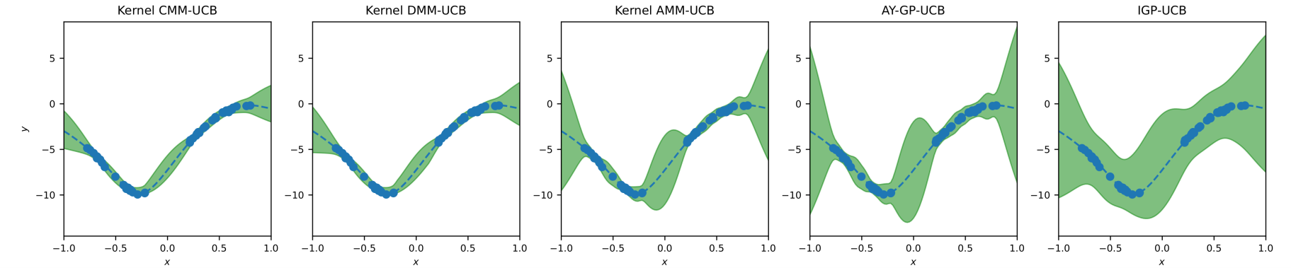
Figure 1: Tighter confidence bounds for sequential kernel regression. The upper and lower confidence bounds used by our Kernel CMM-UCB method (left), the confidence bounds from (Abbasi-Yadkori, 2012) (AY-GP-UCB) (middle-right), and the confidence bounds used by Improved GP-UCB (IGP-UCB) (Chowdhury & Gopalan, 2017) (right) for a Matérn kernel test function with smoothness $\nu=3/2$ and lengthscale $\ell=0.5$. Our Kernel CMM-UCB method – and its relaxed versions DMM-UCB and AMM-UCB – produces confidence bounds that are visibly closer to the ground-truth function (dashed line) than those of AY-GP-UCB and IGP-UCB (cf. also Sec. 6.1).

2 Problem Statement

We consider a sequential kernel regression problem with covariates $x_{t}\in\mathcal{X}$ and responses $y_{t}\in\mathbb{R}$, where

$$y_{t}=f^{*}(x_{t})+\epsilon_{t}.$$

$f^{*}\in\mathcal{H}$ is an unknown function in a reproducing kernel Hilbert space (RKHS) $\mathcal{H}$ and $\epsilon_{1},\epsilon_{2},\dots$ are noise variables. We allow the covariates to be generated in an arbitrary sequential fashion, meaning each $x_{t}$ can depend on $x_{1},y_{1},\dots,x_{t-1},y_{t-1}$. We assume that the RKHS norm of $f^{*}$ is bounded by $B$, i.e. $\left\|f^{*}\right\|_{\mathcal{H}}\leq B$, and that, conditioned on $x_{1},y_{1},\dots,x_{t-1},y_{t-1},x_{t}$, each $\epsilon_{t}$ is $\sigma$-sub-Gaussian.

Our first aim is to construct a confidence sequence for the function $f^{*}$, which we now define formally. For any level $\delta\in(0,1]$, a $(1-\delta)$-confidence sequence is a sequence $\mathcal{F}_{1},\mathcal{F}_{2},\dots$ of subsets of $\mathcal{H}$, such that each $\mathcal{F}_{t}$ can be calculated using the data $x_{1},y_{1},\dots,x_{t},y_{t}$ and the sequence satisfies the coverage condition

$$\mathbb{P}_{\begin{subarray}{c}x_{1},x_{2},\dots\\ y_{1},y_{2},\dots\end{subarray}}\left[\,\forall t\geq 1:\,f^{*}\in\mathcal{F}_{t}\,\right]\,\geq\,1-\delta.$$

In words, this coverage condition says that with high probability, $f^{*}$ lies in $\mathcal{F}_{t}$ for all times $t\geq 1$ simultaneously. We call each set in a confidence sequence a confidence set. Our second aim is to construct confidence bounds for the value of $f^{*}(x)$ at every $x\in\mathcal{X}$. For any level $\delta\in(0,1]$, an anytime-valid $(1-\delta)$-upper confidence bound (UCB) is a sequence $u_{1},u_{2},\dots$ of functions on $\mathcal{X}$, such that each $u_{t}$ can be calculated using the data $x_{1},y_{1},\dots,x_{t},y_{t}$ and the sequence satisfies

$$\mathbb{P}_{\begin{subarray}{c}x_{1},x_{2},\dots\\ y_{1},y_{2},\dots\end{subarray}}\left[\,\forall t\geq 1,\forall x\in\mathcal{X}:f^{*}(x)\leq u_{t}(x)\,\right]\,\geq\,1-\delta.$$

This condition says that with high probability, $u_{t}(x)$ is an upper bound on $f^{*}(x)$ for all $t\geq 1$ and all $x\in\mathcal{X}$ simultaneously. The definition of an anytime-valid lower confidence bound (LCB) is analogous. If we already have a confidence sequence, we can use it to construct upper and lower confidence bounds. In particular, if $\mathcal{F}_{1},\mathcal{F}_{2},\dots$ is a $(1-\delta)$-confidence sequence, then with probability at least $1-\delta$, for all $t\geq 1$ and all $x\in\mathcal{X}$, we have

$$\min_{f\in\mathcal{F}_{t}}\left\{f(x)\right\}\,\leq\,f^{*}(x)\,\leq\,\max_{f\in\mathcal{F}_{t}}\left\{f(x)\right\}.$$ (1)

Therefore, as long as we can solve the maximisation/minimisation problems in (1), we can compute anytime-valid confidence bounds from a confidence sequence. We use $\mathrm{UCB}_{\mathcal{F}_{t}}(x)$ to denote the RHS of (1), i.e. $\mathrm{UCB}_{\mathcal{F}_{t}}(x):=\max_{f\in\mathcal{F}_{t}}\left\{f(x)\right\}$, and $\mathrm{LCB}_{\mathcal{F}_{t}}(x)$ to denote the LHS of (1).

Notation.

For any positive integer $n$, $[n]:=\{1,\dots,n\}$. We use matrix notation to denote the inner product $f_{1}^{\top}f_{2}:=\left\langle f_{1},f_{2}\right\rangle_{\mathcal{H}}$ and outer product $f_{1}f_{2}^{\top}:=f_{1}\left\langle f_{2},\cdot\right\rangle_{\mathcal{H}}$ between two RKHS functions $f_{1},f_{2}\in\mathcal{H}$. We denote the kernel function by $k(\cdot,\cdot)$. For a sequence of observations $x_{1},\dots,x_{t}$, we define $\boldsymbol{k}_{t}(x):=[k(x,x_{1}),\dots,k(x,x_{t})]^{\top}$ and $\Phi_{t}:=[k(x_{1},\cdot),\dots,k(x_{t},\cdot)]^{\top}$. We let $\boldsymbol{K}_{t}:=\{k(x_{i},x_{j})\}_{i\in[t],j\in[t]}=\Phi_{t}\Phi_{t}^{\top}$ denote the kernel matrix and $\boldsymbol{V}_{t}:=\sum_{s=1}^{t}k(\cdot,x_{s})k(\cdot,x_{s})^{\top}=\Phi_{t}^{\top}\Phi_{t}$ the empirical covariance operator. For a parameter $\alpha\geq 0$, we define

$$\mu_{\alpha,t}(x)\, :=\,\boldsymbol{k}_{t}(x)^{\top}(\boldsymbol{K}_{t}+\alpha\boldsymbol{I})^{-1}\boldsymbol{y}_{t},$$ (2)

$$\rho_{\alpha,t}^{2}(x)\, :=\,k(x,x)-\boldsymbol{k}_{t}(x)^{\top}(\boldsymbol{K}_{t}+\alpha\boldsymbol{I})^{-1}\boldsymbol{k}_{t}(x).$$ (3)

$\mu_{\alpha,t}(x)$ is the kernel ridge estimate (evaluated at $x$) or, equivalently, the predictive mean of a standard Gaussian process (GP) posterior with noise $\alpha$. $\rho_{\alpha,t}^{2}(x)$ is the predictive variance of a standard GP posterior.

3 Related Work

Several confidence sequences/bounds have been proposed for the sequential kernel regression problem that we consider. The confidence bounds in (Srinivas et al., 2010) are perhaps the most well-known. The two most widely used, which we compare ours against, were developed by Abbasi-Yadkori et al. (2011); Abbasi-Yadkori (2012) and Chowdhury & Gopalan (2017), using concentration inequalities for self-normalised processes (de la Peña et al., 2004, 2009). Subsequently, Durand et al. (2018) derived empirical Bernstein-type versions of these confidence bounds, and Whitehouse et al. (2023) showed that for certain kernels, these confidence bounds can be tightened by regularising in proportion to the smoothness of the kernel. Confidence sequences for this setting have also been derived using online-to-confidence-set conversions (Abbasi-Yadkori et al., 2012; Abbasi-Yadkori, 2012).

With applications to Bayesian optimisation and kernel bandits in mind, Neiswanger & Ramdas (2021) and Emmenegger et al. (2023) developed confidence sequences using martingale tail bounds for sequential likelihood ratios (assuming Gaussian rather than sub-Gaussian noise). However, cumulative regret bounds for KernelUCB-style bandit algorithms using these confidence bounds are not established in (Neiswanger & Ramdas, 2021), and the regret bound in (Emmenegger et al., 2023) is worse than the one obtained with the confidence bounds in (Abbasi-Yadkori, 2012) or with our new confidence bounds.

The work most closely related to ours is (Flynn et al., 2023), which proposes new confidence bounds for linear bandits, using martingale tail bounds and the method of mixtures. While our Eq. (8) is a simple kernel generalisation of their Eq. (5), deriving confidence bounds is more involved in our kernel setting, because $\max_{f\in\mathcal{F}_{t}}\{f(x)\}$ is now an infinite-dimensional optimisation problem. In their linear (i.e. finite-dimensional) setting, Flynn et al. (2023) bound the regret of their algorithms in terms of the feature vector dimension. The feature dimension is generally infinite in the kernel setting, so we instead bound the regret in terms of the maximum information gain (Srinivas et al., 2010).

4 Confidence Bounds for Kernel Regression

In this section, we use a tail bound for martingale mixtures from (Flynn et al., 2023) to develop tighter confidence sequences and bounds for sequential kernel regression.

4.1 Martingale Mixture Tail Bounds

We begin by recalling the tail bound from Theorem 5.1 of (Flynn et al., 2023) and the general setting in which it holds. We choose a sequence of random functions $(Z_{t}:\mathbb{R}\to\mathbb{R}|t\in\mathbb{N})$ adapted to a filtration $(\mathcal{D}_{t}|t\in\mathbb{N})$, a sequence of predictable “guesses” $(g_{t}\in\mathbb{R}|t\in\mathbb{N})$, and a sequence of predictable random variables $(\lambda_{t}\in\mathbb{R}|t\in\mathbb{N})$. We use the shorthand $\boldsymbol{g}_{t}=[g_{1},\dots,g_{t}]^{\top}$ and $\boldsymbol{\lambda}_{t}=[\lambda_{1},\dots,\lambda_{t}]^{\top}$. Flynn et al. (2023) call a data-dependent sequence of probability distributions $(P_{t}|t\in\mathbb{N})$ an adaptive sequence of mixture distributions if: (a) $P_{t}$ is a distribution over $\boldsymbol{g}_{t}\in\mathbb{R}^{t}$; (b) $P_{t}$ is $\mathcal{D}_{t-1}$-measurable; (c) the distributions are consistent in the sense that their marginals coincide, i.e. $\int P_{t}(\boldsymbol{g}_{t})dg_{t}=P_{t-1}(\boldsymbol{g}_{t-1})$ for all $t$ and $\boldsymbol{g}_{t-1}$. Define

$$M_{t}(\boldsymbol{g}_{t},\boldsymbol{\lambda}_{t}) :=\mathrm{exp}\left(\sum_{s=1}^{t}\lambda_{s}Z_{s}(g_{s})-\psi_{s}(g_{s},\lambda_{s})\right),$$ (4)

$$\psi_{t}(g_{t},\lambda_{t}) :=\ln\left(\mathbb{E}\left[\mathrm{exp}(\lambda_{t}Z_{t}(g_{t}))|\mathcal{D}_{t-1}\right]\right),$$ (5)

Flynn et al. (2023) show that $M_{t}(\boldsymbol{g}_{t},\boldsymbol{\lambda}_{t})$ is a non-negative martingale, and that, due to conditions (a)-(c) on the mixture distributions, the mixture $\mathbb{E}_{\boldsymbol{g}_{t}\sim P_{t}}\left[M_{t}(\boldsymbol{g}_{t},\boldsymbol{\lambda}_{t})\right]$ is also a non-negative martingale. This means that Ville’s inequality (Ville, 1939) can be applied. Thm. 5.1 in (Flynn et al., 2023) provides a time-uniform tail bound for the martingale mixture $\mathbb{E}_{\boldsymbol{g}_{t}\sim P_{t}}\left[M_{t}(\boldsymbol{g}_{t},\boldsymbol{\lambda}_{t})\right]$.

Theorem 4.1 (Tail Bound for Adaptive Martingale Mixtures (Theorem 5.1 of (Flynn et al., 2023)).

For any $\delta\in(0,1)$, any adaptive sequence of mixture distributions $(P_{t}|t\in\mathbb{N})$, and any sequence of predictable random variables $(\lambda_{t}|t\in\mathbb{N})$, it holds with probability at least $1-\delta$ that

$$\forall t\geq 1:\quad\mathrm{ln}\left(\mathop{\mathbb{E}}_{\boldsymbol{g}_{t}\sim P_{t}}\left[M_{t}(\boldsymbol{g}_{t},\boldsymbol{\lambda}_{t})\right]\right)\,\leq\,\mathrm{ln}(1/\delta).$$ (6)

We choose $(\mathcal{D}_{t}|t\in\mathbb{N})$ to be any filtration such that $y_{t}$ and $x_{t+1}$ are both $\mathcal{D}_{t}$-measurable, e.g. $\mathcal{D}_{t}=\sigma(x_{1},y_{1},\dots,x_{t},y_{t},x_{t+1})$. Focusing on linear bandits, Flynn et al. (2023) choose $Z_{t}(g_{t})=(g_{t}-\phi(x_{t})^{\top}\boldsymbol{\theta}^{*})\epsilon_{t}$, where $\phi(\cdot)^{\top}\boldsymbol{\theta}^{*}$ is a linear reward function, and show that under this choice, Eq. (6) reduces to a convex constraint for the finite-dimensional parameter vector $\boldsymbol{\theta}^{*}$. In our kernel setting, we choose $Z_{t}(g_{t})=(g_{t}-f^{*}(x_{t}))\epsilon_{t}$, leading to a convex constraint for the function $f^{*}$. As $Z_{t}(g_{t})$ is linear in the noise variable $\epsilon_{t}$, $\psi_{t}(g_{t},\lambda_{t})$ can be upper bounded using the $\sigma$-sub-Gaussian property of $\epsilon_{t}$.

$$\psi_{t}(g_{t},\lambda_{t})\,\leq\,\tfrac{1}{2}\sigma^{2}\lambda_{t}^{2}(g_{t}-f^{*}(x_{t}))^{2}.$$

Using this upper bound, choosing $\lambda_{t}\equiv 1/\sigma^{2}$, and rearranging Eq. (6) (see App. A.1), we obtain an upper bound on the Euclidean distance between the vector of ground-truth function values $\boldsymbol{f}_{t}^{*}:=[f^{*}(x_{1}),\dots,f^{*}(x_{t})]^{\top}$ and the observed response vector $\boldsymbol{y}_{t}:=[y_{1},\dots,y_{t}]^{\top}$.

$$\begin{split}&\|\boldsymbol{f}_{t}^{*}-\boldsymbol{y}_{t}\|_{2}^{2}~{}\leq~{}2\sigma^{2}\ln(1/\delta)\\ &\quad-2\sigma^{2}\ln\left(\mathop{\mathbb{E}}_{\boldsymbol{g}_{t}\sim P_{t}}\left[\mathrm{exp}\left(-\frac{1}{2\sigma^{2}}\|\boldsymbol{g}_{t}-\boldsymbol{y}_{t}\|_{2}^{2}\right)\right]\right).\end{split}$$ (7)

Next, we choose the mixture distributions $P_{t}=\mathcal{N}(\boldsymbol{0},c\boldsymbol{K}_{t})$, resembling a zero-mean Gaussian process with covariance scaled by $c>0$. There are several reasons for this choice of $P_{t}$. First, for an appropriate covariance scale $c>0$, we prove that the confidence bounds obtained from (7) with $P_{t}=\mathcal{N}(\boldsymbol{0},c\boldsymbol{K}_{t})$ are always tighter than those in (Abbasi-Yadkori, 2012) and (Chowdhury & Gopalan, 2017) (see Sec. 6.1). Second, any Gaussian $P_{t}$ yields a convenient closed-form expression for the expected value in (7) (see App. A.2). Substituting this expression into (7), we obtain

$$\|\boldsymbol{f}_{t}^{*}-\boldsymbol{y}_{t}\|_{2}^{2}~{}\leq ~{}\,\boldsymbol{y}_{t}^{\top}\left(\boldsymbol{I}+\frac{c\boldsymbol{K}_{t}}{\sigma^{2}}\right)^{-1}\boldsymbol{y}_{t}$$ (8)

$$+\sigma^{2}\ln\det\left(\boldsymbol{I}+\frac{c\boldsymbol{K}_{t}}{\sigma^{2}}\right)+2\sigma^{2}\ln\frac{1}{\delta}$$

$$=:R_{t}^{2}.$$

This inequality states that with probability at least $1-\delta$, at every step $t$, the vector of ground-truth function values $\boldsymbol{f}_{t}^{*}$ lies within a sphere of radius $R_{t}$ around the observed response vector $\boldsymbol{y}_{t}$.

4.2 Confidence Sequences

We now describe how the tail bound in (8) can be used to construct confidence sequences for $f^{*}$. Let $\boldsymbol{f}_{t}=[f(x_{1}),\dots,f(x_{t})]^{\top}$ denote the values of an arbitrary function $f\in\mathcal{H}$ at the points $x_{1},\dots,x_{t}$. Since, with probability at least $1-\delta$, (8) holds for all $t\geq 1$, the sets of functions $f\in\mathcal{H}$ that (at each $t$) satisfy both (8) and $\left\|f\right\|_{\mathcal{H}}\leq B$ form a $1-\delta$ confidence sequence for $f^{*}$.

Lemma 4.2 (Confidence sequence).

For any $c>0$ and $\delta\in(0,1]$, it holds with probability at least $1-\delta$ that for all $t\geq 1$ simultaneously, the function $f^{*}$ lies in the set

$$\mathcal{F}_{t}=\bigg{\{}f\in\mathcal{H}\,\bigg{|}\, \|\boldsymbol{f}_{t}-\boldsymbol{y}_{t}\|_{2}\leq R_{t},~{}\left\|f\right\|_{\mathcal{H}}\leq B\bigg{\}}.$$

The two constraints that define $\mathcal{F}_{t}$ are both ellipsoids in $\mathcal{H}$, meaning that $\mathcal{F}_{t}$ is an intersection of two ellipsoids. In contrast, most existing confidence sets for functions in RKHS’s (e.g. (Abbasi-Yadkori, 2012; Chowdhury & Gopalan, 2017)) are single ellipsoids centred at the kernel ridge estimate $\mu_{\alpha,t}$ (see Eq. (2)), for some regularisation parameter $\alpha>0$. It turns out that by taking a weighted sum of the constraints in $\mathcal{F}_{t}$, we can obtain a single-ellipsoid confidence set $\widetilde{\mathcal{F}}_{t}\supseteq\mathcal{F}_{t}$, which is also centred at the kernel ridge estimate.

Corollary 4.3.

For any $c>0$, any $\alpha>0$ and any $\delta\in(0,1]$, it holds with probability at least $1-\delta$ that for all $t\geq 1$ simultaneously, $f^{*}$ lies in the set

$$\widetilde{\mathcal{F}}_{t}=\left\{f\in\mathcal{H}\,\bigg{|}\,\left\|\left(\boldsymbol{V}_{t}+\alpha\boldsymbol{I}_{\mathcal{H}}\right)^{1/2}(f-\mu_{\alpha,t})\right\|_{\mathcal{H}}\leq\widetilde{R}_{\alpha,t}\right\},$$

where

$$\widetilde{R}_{\alpha,t}^{2}:=R_{t}^{2}+\alpha B^{2}-\boldsymbol{y}_{t}^{\top}\boldsymbol{y}_{t}+\boldsymbol{y}_{t}^{\top}\Phi_{t}(\boldsymbol{V}_{t}+\alpha\boldsymbol{I}_{\mathcal{H}})^{-1}\Phi_{t}^{\top}\boldsymbol{y}_{t}.$$

The proof (in App. B.2) involves rearranging the inequality

$$\|\boldsymbol{f}_{t}-\boldsymbol{y}_{t}\|_{2}^{2}+\alpha\left\|f\right\|_{\mathcal{H}}^{2}~{}\leq~{}R_{t}^{2}+\alpha B^{2},$$

into the constraint that defines $\widetilde{\mathcal{F}}_{t}$. This larger confidence sequence can be more easily compared to those in (Abbasi-Yadkori, 2012; Chowdhury & Gopalan, 2017), cf. Sec. 6.1.

4.3 Implicit Confidence Bounds

We now turn our attention to the confidence bounds that can be obtained from our confidence sequences, and how we can compute them. We start by considering the exact upper confidence bound $\mathrm{UCB}_{\mathcal{F}_{t}}(x)=\max_{f\in\mathcal{F}_{t}}\left\{f(x)\right\}$, which can be written as

$$\max_{f\in\mathcal{H}}\;f(x)~{}~{}\text{s.t.}~{}~{}\|\boldsymbol{f}_{t}-\boldsymbol{y}_{t}\|_{2}\leq R_{t},~{}~{}\left\|f\right\|_{\mathcal{H}}\leq B.$$ (9)

The optimisation variable in (9) is a function in the possibly infinite-dimensional RKHS $\mathcal{H}$, which makes it difficult to directly compute the numerical solution of (9). We now describe two finite-dimensional reformulations of (9).

As (9) contains a constraint on the RKHS norm of $f$, the (generalised) representer theorem (Kimeldorf & Wahba, 1971; Schölkopf et al., 2001) can be applied. This means that the solution of (9) can be expressed as a finite linear combination of the form $\boldsymbol{k}_{t+1}(x)^{\top}\boldsymbol{w}$, where $\boldsymbol{k}_{t+1}(x):=[k(x,x_{1}),\dots,k(x,x_{t}),k(x,x)]^{\top}$. When we substitute the functional form $f(\cdot)=\boldsymbol{k}_{t+1}(\cdot)^{\top}\boldsymbol{w}$ into the objective and both constraints, we obtain the finite-dimensional convex program in Thm. 4.4. (see App. B.3).

Theorem 4.4 (Representer theorem for UCB computation).

$\mathrm{UCB}_{\mathcal{F}_{t}}(x)$ equals the solution of the convex program

$$\max_{\boldsymbol{w}\in\mathbb{R}^{t+1}} ~{}\boldsymbol{k}_{t+1}(x)^{\top}\boldsymbol{w}$$ (10)

s.t. $$\|\boldsymbol{K}_{t,t+1}\boldsymbol{w}-\boldsymbol{y}_{t}\|_{2}\leq R_{t},$$

$$\|\boldsymbol{L}_{t+1}\boldsymbol{w}\|_{2}\leq B.$$

where $\boldsymbol{K}_{t,t+1}:=(\boldsymbol{K}_{t},\boldsymbol{k}_{t}(x))\in\mathbb{R}^{t\times(t+1)}$ denotes kernel matrix with added last column $\boldsymbol{k}_{t}(x)$, and $\boldsymbol{L}_{t+1}$ is any matrix satisfying $\boldsymbol{L}_{t+1}^{\top}\boldsymbol{L}_{t+1}=\boldsymbol{K}_{t+1}$ (e.g. the right Cholesky factor of $\boldsymbol{K}_{t+1}$).

Eq. (10) is a $(t+1)$-dimensional second order cone program, which can be solved efficiently using conic solvers from, for example, the CVXPY library (Diamond & Boyd, 2016). To illustrate the simplicity of solving (10) with such libraries, we provide sample code in App. E.1. For our second reformulation, we focus on the Lagrangian dual problem associated with (9).

Theorem 4.5 (Dual problem for UCB computation).

The dual problem associated with (9) is

$$\min_{\begin{subarray}{c}\eta_{1}>0\\ \eta_{2}>0\end{subarray}}\left\{\mu_{\eta_{2}/\eta_{1},t}(x)-\frac{\rho_{\eta_{2}/\eta_{1},t}^{2}(x)}{4\eta_{2}}+\eta_{1}\widetilde{R}_{\eta_{2}/\eta_{1},t}^{2}\right\}.$$ (11)

See (2) and (3) for the definitions of $\mu_{\eta_{2}/\eta_{1},t}(x)$ and $\rho_{\eta_{2}/\eta_{1},t}^{2}(x)$. We provide a proof in App. B.4 and focus here on the consequences of this result. By weak duality, the solution of (11) is always an upper bound on the solution of the primal problem in (9). Whenever there exists an $f$ that lies in the interior of the ellipsoids that define $\mathcal{F}_{t}$, as is usually the case, then strong duality holds and the solutions of (9) and (11) are actually equal. In App. B.4, we show that (11) can be further reduced to a one-dimensional optimisation problem. Using the substitution $\eta_{2}=\alpha\eta_{1}$ (for $\alpha>0$), the solution of (11) is equal to

$$\min_{\alpha>0}\left\{\mu_{\alpha,t}(x)+\frac{\widetilde{R}_{\alpha,t}}{\sqrt{\alpha}}\rho_{\alpha,t}(x)\right\}.$$ (12)

The objective function in (12) is not always convex in $\alpha$, though empirical evidence suggests that it is quasiconvex in $\alpha$, and could therefore be solved using the bisection method. Since $\mu_{\alpha,t}(x)$ is the predictive mean of a standard Gaussian process (GP) posterior and $\rho_{\alpha,t}^{2}(x)$ is its predictive variance, the objective function in (12) closely resembles GP-based confidence bounds (e.g. (Srinivas et al., 2010)). We can therefore interpret our confidence bound $\mathrm{UCB}_{\mathcal{F}_{t}}(x)$ as a GP-based confidence bound, which is minimised with respect to the regularisation parameter.

4.4 Explicit Confidence Bounds

In this section, we focus on explicit confidence bounds. These confidence bounds are mainly useful for deriving worst-case regret bounds with explicit dependence on $T$ (see Section 6.2), but are also cheaper to compute than the implicit confidence bounds in the previous subsection. From (12) in the previous subsection, we can immediately see that for any fixed $\alpha>0$, we have

$$\mathrm{UCB}_{\mathcal{F}_{t}}(x)~{}\leq~{}\mu_{\alpha,t}(x)+\frac{\widetilde{R}_{\alpha,t}}{\sqrt{\alpha}}\rho_{\alpha,t}(x).$$ (13)

It turns out that this upper bound on $\mathrm{UCB}_{\mathcal{F}_{t}}(x)$ is equal to the confidence bound $\mathrm{UCB}_{\widetilde{\mathcal{F}}_{t}}(x)$, where $\widetilde{\mathcal{F}}_{t}$ is the confidence set from Lemma 4.3.

Corollary 4.6 (Analytic UCB).

For all $t\geq 1$ and $x\in\mathcal{X}$,

$$\mathrm{UCB}_{\widetilde{\mathcal{F}}_{t}}(x)~{}\leq~{}\mu_{\alpha,t}(x)+\frac{\widetilde{R}_{\alpha,t}}{\sqrt{\alpha}}\rho_{\alpha,t}(x).$$ (14)

This statement follows from the proof of Thm. 11. In particular, one can show that the RHS of (14) is the solution of the dual problem associated with $\max_{f\in\widetilde{\mathcal{F}}_{t}}\{f(x)\}$. Again, when $\widetilde{\mathcal{F}}_{t}$ has an interior point (as is usually the case), the inequality in (14) is actually an equality. The inequality in Cor. 4.6 also follows from Cauchy-Schwarz (App. B.5).

4.5 Confidence Bound Maximisation

We now discuss how our upper confidence bounds can be maximised w.r.t. $x\in\mathcal{X}$, which is an important consideration for kernel bandits (see Sec. 5). If $\mathcal{X}$ has finite (and not too large) cardinality, then $\mathrm{UCB}_{\mathcal{F}_{t}}(x)$ (and upper bounds on it) can easily be maximised exactly.

If $\mathcal{X}$ is a continuous subset of $\mathbb{R}^{d}$, then maximising $\mathrm{UCB}_{\mathcal{F}_{t}}(x)$ or any of our upper bounds over $x$ exactly is intractable in general, though other similar confidence bounds have the same limitation. There are at least two options for approximate maximisation. One option is to use gradient-based methods as in (Flynn et al., 2023). Gradients (w.r.t. $x$) of the implicit confidence bounds in (10), (11) and (12) can be computed numerically using differentiable convex optimsation methods (Agrawal et al., 2019) or automatic implicit differentiation methods (Look et al., 2020; Blondel et al., 2022). Gradient-based maximisation works well in practice, even though there are no rigorous approximation guarantees as $\mathrm{UCB}_{\mathcal{F}_{t}}(x)$ is (in general) a non-concave function of $x$. The second option is to discretise $\mathcal{X}$ and optimise over the finite discretisation (see e.g. Sec. 3.1 of (Li & Scarlett, 2022)). When the kernel function $k(x,x^{\prime})$ is Lipschitz (as the RBF and Matérn kernels are), then the discretisation error can be controlled. However, the grid size for a sufficiently fine discretisation grows exponentially in the dimension $d$ of $\mathcal{X}$, so this quickly becomes impractical.

5 Application To Kernel Bandits

To demonstrate the utility of our confidence bounds, we apply them to the stochastic kernel bandit problem.

5.1 Stochastic Kernel Bandits

A learner plays a game over a sequence of $T$ rounds, where $T$ may not be known in advance. In each round $t$, the learner observes an action set $\mathcal{X}_{t}\subseteq\mathcal{X}$ and must choose an action $x_{t}\in\mathcal{X}_{t}$. The learner then receives a reward $y_{t}=f^{*}(x_{t})+\epsilon_{t}$. The reward function $f^{*}:\mathcal{X}\to\mathbb{R}$ is an unknown function in an RKHS. As before, we assume that $f^{*}$ has bounded RKHS norm, i.e. $\left\|f^{*}\right\|_{\mathcal{H}}\leq B$, and that $\epsilon_{1},\epsilon_{2},\dots,\epsilon_{T}$ are conditionally $\sigma$-sub-Gaussian.

The goal of the learner is to choose a sequence of actions that minimises cumulative regret, which is the difference between the total expected reward of the learner and the optimal strategy. For a single round, we define the regret as $r_{t}=f^{*}(x_{t}^{*})-f^{*}(x_{t})$, where $x_{t}^{*}=\operatornamewithlimits{argmax}_{x\in\mathcal{X}_{t}}\{f^{*}(x)\}$. After $T$ rounds, the cumulative regret is $r_{1:T}=\sum_{t=1}^{T}r_{t}$.

5.2 Kernel UCB Meta Algorithm

In Algorithm 1, we describe a general recipe for a kernel bandit algorithm, which is based on a sequence of upper confidence bounds $u_{0},u_{1},u_{2},\dots$ for the reward function $f^{*}$. In each round $t$, we use all previous observations $\{(x_{s},y_{s})\}_{s=1}^{t-1}$ to successively construct the UCB $u_{t-1}$, and then select the action that maximises $u_{t-1}$.

Algorithm 1 KernelUCB

  Input: Upper confidence bounds $u_{0},u_{1},u_{2},\dots$

  for $t=1$ to $T$ do

     Play $x_{t}=\operatornamewithlimits{argmax}_{x\in\mathcal{X}_{t}}\{u_{t-1}(x)\}$

     Observe $y_{t}=f^{*}(x_{t})+\epsilon_{t}$

  end for

For each $t$, we must be able to compute $u_{t}$ using the data $x_{1},y_{1},\dots,x_{t},y_{t}$. Kernel bandit algorithms of this form have appeared under different names, such as GP-UCB (Srinivas et al., 2010) and KernelUCB (Valko et al., 2013), based on the confidence bounds that they use. We therefore use the names KernelUCB and GP-UCB synonymously. When we use the confidence bounds in Thm. 3.11 of (Abbasi-Yadkori, 2012), we call Algorithm 1 AY-GP-UCB. If we use the confidence bounds in Thm. 2 of (Chowdhury & Gopalan, 2017), then Algorithm 1 is the Improved GP-UCB algorithm (IGP-UCB).

5.3 Kernel CMM-UCB

For our first variant of KernelUCB, we use our exact confidence bound $\mathrm{UCB}_{\mathcal{F}_{t}}(x)$. In particular, we set $u_{t}(x)$ to be the numerical solution of (10). The resulting algorithm, which we call Kernel Convex Martingale Mixture UCB (Kernel CMM-UCB), is a kernelised version of the CMM-UCB algorithm for linear bandits (Flynn et al., 2023).

5.4 Kernel DMM-UCB

For our second variant of KernelUCB, we use the confidence bound in (12) that comes from the dual problem associated with $\max_{f\in\mathcal{F}_{t}}\{f(x)\}$. In the interest of computational efficiency, we replace $\min_{\alpha>0}$ in (12) with $\min_{\alpha\in A}$, for a small grid $A$ of values of $\alpha$. In particular, we set

$$u_{t}(x)=\min_{\alpha\in A}\left\{\mu_{\alpha,t}(x)+\frac{\widetilde{R}_{\alpha,t}}{\sqrt{\alpha}}\rho_{\alpha,t}(x)\right\}.$$

We call the resulting bandit algorithm Kernel Dual Martingale Mixture UCB (Kernel DMM-UCB). Because we only optimise $\alpha$ over the grid $A$, this upper confidence bound is looser than the exact confidence bound used by Kernel CMM-UCB. In return, the cost of computing this UCB is only a factor of $|A|$ more than the cost of computing the analytic UCB in Cor. 4.6.

5.5 Kernel AMM-UCB

For our third and final variant of KernelUCB, we set $u_{t}(x)$ to be the analytic UCB from Cor. 4.6 with a fixed value of $\alpha$. The resulting algorithm, which we call Kernel Analytic Martingale Mixture UCB (Kernel AMM-UCB), is a kernelised version of the AMM-UCB algorithm for linear bandits (Flynn et al., 2023). This algorithm is mainly useful for our regret analysis in Section 6.2.

6 Theoretical Analysis

Table 1: Cumulative regret of our KernelUCB-style algorithms as well as AY-GP-UCB, IGP-UCB and a random baseline after $T=1000$ rounds with $d=3$. We show the mean $\pm$ standard deviation over 10 repetitions.

	RBF Kernel		Matérn Kernel ($\nu=5/2$)		Matérn Kernel ($\nu=3/2$)
	$\ell=0.5$	$\ell=0.2$	$\ell=0.5$	$\ell=0.2$	$\ell=0.5$	$\ell=0.2$
Kernel DMM-UCB (Ours)	32.2 $\pm$ 20.9	491.4 $\pm$ 117.1	129.5 $\pm$ 45.6	795.1 $\pm$ 206.0	195.6 $\pm$ 78.0	814.1 $\pm$ 344.4
Kernel AMM-UCB (Ours)	88.8 $\pm$ 6.1	1206.2 $\pm$ 20.8	197.0 $\pm$ 24.4	1661.5 $\pm$ 90.1	316.1 $\pm$ 51.1	1741.2 $\pm$ 351.2
AY-GP-UCB	136.9 $\pm$ 12.7	1518.4 $\pm$ 38.9	331.7 $\pm$ 45.2	2382.4 $\pm$ 135.4	546.0 $\pm$ 70.0	2421.3 $\pm$ 568.5
IGP-UCB	314.1 $\pm$ 110.5	1433.0 $\pm$ 122.8	553.3 $\pm$ 67.5	1853.1 $\pm$ 105.7	655.6 $\pm$ 67.4	1707.5 $\pm$ 375.5
Random	4282.4 $\pm$ 1015.4	3872.4 $\pm$ 783.7	4264.7 $\pm$ 778.0	3677.5 $\pm$ 559.2	4175.1 $\pm$ 681.0	3442.0 $\pm$ 1080.4

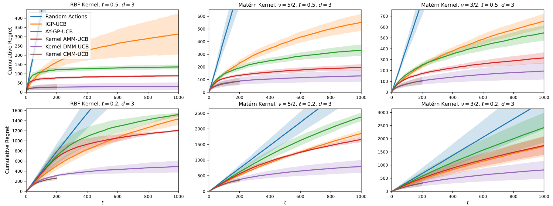
Figure 2: Cumulative regret of our KernelUCB-style algorithms as well as AY-GP-UCB, IGP-UCB and a random baseline over $T=1000$ rounds for $d=3$ and various kernels (columns) and length scales (rows). We show the mean $\pm$ standard deviation over 10 repetitions.

In this section, we show that our analytic confidence bound from Cor. 4.6 is always tighter than the confidence bounds in Thm. 3.11 of (Abbasi-Yadkori, 2012) and Thm. 2 of (Chowdhury & Gopalan, 2017), which hold under the same conditions and assumptions. In addition, we establish cumulative regret bounds for Kernel CMM-UCB, Kernel DMM-UCB and Kernel AMM-UCB. We begin by formally stating the assumptions under which our analysis holds. We assume that the noise variables are conditionally $\sigma$-sub-Gaussian.

Assumption 6.1 (Sub-Gaussian noise).

Let $(\mathcal{D}_{t}|t\in\mathbb{N})$ be any filtration such that $y_{t}$ and $x_{t+1}$ are both $\mathcal{D}_{t}$-measurable. Each noise variable $\epsilon_{t}$ is conditionally $\sigma$-sub-Gaussian, which means

$$\forall\lambda\in\mathbb{R},\;\ \mathbb{E}\left[\mathrm{exp}(\lambda\epsilon_{t})|\mathcal{D}_{t-1}\right]\leq\mathrm{exp}(\lambda^{2}\sigma^{2}/2).$$

This condition implies that $\mathbb{E}\left[\epsilon_{t}|\mathcal{D}_{t-1}\right]=0$. We assume that the reward function is uniformly bounded, and that its RKHS norm is bounded.

Assumption 6.2 (Bounded reward function).

For some $B>0$, $\left\|f^{*}\right\|_{\mathcal{H}}\leq B$. For some $C>0$, $\sup_{x\in\mathcal{X}}|f^{*}(x)|\leq C$.

If the kernel function is uniformly bounded by some $\kappa>0$, i.e. $k(x,x^{\prime})\in[-\kappa,\kappa]$ for all $x,x^{\prime}\in\mathcal{X}$, then $\left\|f^{*}\right\|_{\mathcal{H}}\leq B$ implies that $f^{*}(x)\in[-C,C]$ holds with $C\leq\kappa B$. To compute our confidence bounds and run our bandit algorithms, we do not need to know the value of $C$, but we do need to know (upper bounds on) $\sigma$ and $B$.

6.1 Tighter Confidence Bounds

The confidence bounds in (Abbasi-Yadkori, 2012) and (Chowdhury & Gopalan, 2017) are the same as our analytic UCB in (14), except that the (scaled) radius $\widetilde{R}_{\alpha,t}/\sqrt{\alpha}$ is replaced with a different quantity. For any values of the regularisation parameters $\lambda>0$ and $\eta>0$ used in (Abbasi-Yadkori, 2012) and (Chowdhury & Gopalan, 2017) respectively, we show that we can set $c$ and $\alpha$ such that $\widetilde{R}_{\alpha,t}/\sqrt{\alpha}$ is strictly less than these other radius quantities. This result is stated in Thm. 6.3 and proved in App. C.2.

Theorem 6.3.

For every $\delta\in(0,1]$ and every value of the regularisation parameter $\lambda>0$, the RHS of (14) with $c=\sigma^{2}/\lambda$ and $\alpha=\lambda$ is strictly less than the UCB in Thm. 3.11 of (Abbasi-Yadkori, 2012).

For every $\delta\in(0,1]$ and every value of the regularisation parameter $\eta>0$, the RHS of (14) with $c=\sigma^{2}/(1+\eta)$ and $\alpha=1+\eta$ is strictly less than the UCB in Thm. 2 of (Chowdhury & Gopalan, 2017).

6.2 Cumulative Regret Bounds

We bound cumulative regret in terms of a kernel-dependent quantity called the maximum information gain, which is defined as

$$\gamma_{t}(\alpha):=\max_{x_{1},\dots,x_{t}}\left\{\frac{1}{2}\ln\left(\det\left(\frac{1}{\alpha}\boldsymbol{K}_{t}+\boldsymbol{I}\right)\right)\right\}.$$

First, we need to upper bound our radius quantity $\widetilde{R}_{\alpha,t}$ in terms of the maximum information gain. To do so, we show that when $\alpha=\sigma^{2}/c$, the quadratic terms in $\widetilde{R}_{\alpha,t}$ cancel out (see Lemma C.2), and we are left with

$$\widetilde{R}_{\sigma^{2}/c,t} \leq\sqrt{2\sigma^{2}\gamma_{t}(\sigma^{2}/c)+\tfrac{\sigma^{2}B^{2}}{c}+2\sigma^{2}\ln(\tfrac{1}{\delta})}.$$

We now proceed to upper bound the cumulative regret of Kernel AMM-UCB with $\alpha=\sigma^{2}/c$. Using a standard argument (see e.g. Prop. 1 in (Russo & Van Roy, 2013) and also Lemma D.1 in App. D.1), the regret of any UCB algorithm at round $t$ is (with high probability) upper bounded by the difference between the upper and lower confidence bounds (at $x_{t}$) that it uses. For Kernel AMM-UCB, this bound is

$$r_{t}\leq\frac{2\widetilde{R}_{\sigma^{2}/c,t-1}}{\sqrt{\sigma^{2}/c}}\rho_{\sigma^{2}/c,t-1}(x_{t}).$$ (15)

From here, our cumulative regret bound in Thm. 6.4 follows from standard arguments, so we defer the proof to App. D.2.

Theorem 6.4.

For any covariance scale $c>0$, with probability at least $1-\delta$, for all $T\geq 1$, the cumulative regret of Kernel CMM-UCB, Kernel DMM-UCB (with a grid $A$ containing $\alpha=\sigma^{2}/c$) and Kernel AMM-UCB (with $\alpha=\sigma^{2}/c$) satisfies

$$r_{1:T}=\mathcal{O}\left(\sqrt{T\gamma_{T}(\tfrac{\sigma^{2}}{c})\left(\gamma_{T}(\tfrac{\sigma^{2}}{c})+\tfrac{1}{c}B^{2}+\ln(\tfrac{1}{\delta})\right)}\right).$$

Because the confidence bounds used by Kernel CMM-UCB (with the same $c$) and Kernel DMM-UCB (with the same $c$ and with $\alpha=\sigma^{2}/c\in A$) are never looser than the confidence bounds used by Kernel AMM-UCB, these algorithms also satisfy the bound in (15), which means the cumulative regret bound for Kernel AMM-UCB also applies to Kernel CMM-UCB and Kernel DMM-UCB.

The regret bound in Thm. 6.4 matches the best existing regret bounds for bandit algorithms that follow the KernelUCB recipe in Algorithm 1 (Srinivas et al., 2010; Chowdhury & Gopalan, 2017; Durand et al., 2018; Whitehouse et al., 2023), though its dependence on the maximum information gain is sub-optimal by a factor of $\sqrt{\gamma_{T}}$. However, due to the lower bound in (Lattimore, 2023), this cannot be improved by using a better confidence sequence for $f^{*}$.

For the frequently used RBF and Matérn kernels, the dependence of the maximum information gain on $T$ can be made explicit. For the RBF kernel and with $c\propto 1$, the maximum information gain is $\mathcal{O}((\ln(T))^{d+1})$ (see e.g. (Srinivas et al., 2010; Vakili et al., 2021)), which means the regret bound in Thm. 6.4 is $\mathcal{O}(\sqrt{T}(\ln(T))^{d+1})$. For the Matérn kernel with smoothness parameter $\nu$ and $c\propto T^{-\frac{d}{2d+2\nu}}$, the maximum information gain is $\mathcal{O}(T^{\frac{d}{2d+2\nu}}(\ln(T))^{\frac{2\nu}{2d+2\nu}})$ (see e.g. (Vakili et al., 2021; Whitehouse et al., 2023)), which means the regret bound is $\mathcal{O}(T^{\frac{2d+\nu}{2d+2\nu}}(\ln(T))^{\frac{2\nu}{d+2\nu}})$.

7 Experiments

We aim to verify that when our confidence bounds replace existing ones, KernelUCB shows better empirical performance at a similar computational cost.

Compared Methods.

We compare: a) Kernel CMM-UCB: cf. Sec. 5.3; b) Kernel DMM-UCB: cf. Sec. 5.4; c) Kernel AMM-UCB: cf. Sec. 5.5; d) AY-GP-UCB: Algorithm 1 with the confidence bounds from Thm. 3.11 of (Abbasi-Yadkori, 2012); e) IGP-UCB: Algorithm 1 with the confidence bounds from Thm. 2 of (Chowdhury & Gopalan, 2017); e) Random: Actions are chosen uniformly at random.

Experimental Setup.

We run each algorithm in several synthetic kernel bandit problems. To generate each reward function, we sample 20 inducing points $z_{1},\dots,z_{20}$ uniformly at random from the hypercube $[0,1]^{d}$ and a 20-dimensional weight vector $\boldsymbol{w}\in\mathbb{R}^{20}$ from a standard normal distribution. The test function is $f^{*}(x)=b\sum_{i=1}^{20}w_{i}k(x,z_{i})$, where the scaling factor $b$ is set such that $\left\|f^{*}\right\|_{\mathcal{H}}=B$. The noise variables $\epsilon_{1},\epsilon_{2},\dots$ are drawn independently from a normal distribution with mean 0 and standard deviation $\sigma$. In each round $t$, the action set $\mathcal{X}_{t}$ consists of 100 $d$-dimensional vectors drawn uniformly at random from the hypercube $[0,1]^{d}$. We present results for $d\in\{2,3,4\}$ and with the RBF and Matérn kernels with length scale $\ell\in\{0.2,0.5\}$. We record the cumulative regret and wall-clock time-per-step over $T=1000$ rounds.

We run each algorithm with $\delta=0.01$ and the true values $B=10$ and $\sigma=0.1$. We run IGP-UCB with the recommend value of $\eta=2/T$. For each of our methods, we set the covariance scale to $c=1$ for the RBF kernel and $c=T^{-\frac{d}{2d+2\nu}}$ for the Matérn kernel. Equivalently, for AY-GP-UCB, we set $\lambda=\sigma^{2}$ for the RBF kernel and $\lambda=\sigma^{2}T^{\frac{d}{2d+2\nu}}$ for the Matérn kernel. We run Kernel AMM-UCB with $\alpha=\sigma^{2}/c$ and Kernel DMM-UCB with $A=\{0.1\sigma^{2}/c,0.3\sigma^{2}/c,\sigma^{2}/c,3\sigma^{2}/c,10\sigma^{2}/c\}$. Due to prohibitive cost, we only run Kernel CMM-UCB for 200 rounds. All experiments were run on a single computer with an Intel i5-1145G7 CPU.

Results.

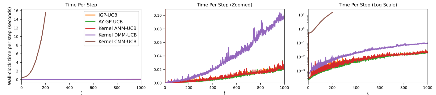
Figure 4: Wall-clock time per step for our kernel UCB-style algorithms as well as AY-GP-UCB, IGP-UCB over $T=1000$ rounds with: (left) original $y$-axis; (middle) zoomed-in $y$-axis; (right) log scale $y$-axis. We show the mean over 10 repetitions.

Fig. 2 shows the cumulative regret of each algorithm with $d=3$, every kernel and every length-scale (results with $d\in\{2,4\}$ are shown in App. F.2). The cumulative regret at $T=1000$ is displayed in Tab. 1. Our Kernel CMM-UCB algorithm consistently achieves the lowest cumulative regret over the first 200 steps. Our Kernel DMM-UCB algorithm closely matches Kernel CMM-UCB over the first 200 steps and consistently achieves the lowest cumulative regret over 1000 steps. Fig. 4 (in App. F.1) shows the wall-clock time per step for each method. IGP-UCB, AY-GP-UCB and Kernel AMM-UCB take approximately the same time per step. As we would expect, since we used a grid $A$ of size 5, the time per step for Kernel DMM-UCB is a little under 5 times that of Kernel AMM-UCB. The time per step for Kernel CMM-UCB grows at the fastest rate in $t$. At $t=200$, the time per step for Kernel CMM-UCB is more than 15 seconds, whereas the time per step for every other method is below 0.02 seconds.

8 Conclusion

In this paper, we developed new confidence sequences and confidence bounds for sequential kernel regression. In our theoretical analysis, we proved that our new confidence bounds are always tighter than comparable existing confidence bounds. We presented three variants of the KernelUCB algorithm for kernel bandits, which each use different confidence bounds that can be derived from our confidence sequences. The results of our experiments suggest that the Kernel DMM-UCB algorithm should be the preferred choice for practical uses. It closely matches the empirical performance of our effective but expensive Kernel CMM-UCB algorithm, yet it has roughly the same computational cost as our Kernel AMM-UCB method (as well as AY-GP-UCB and IGP-UCB). Together, our theoretical analysis and our experiments suggest that by replacing existing confidence bounds in KernelUCB with our new confidence bounds, we obtain kernel bandit algorithms with better empirical performance, matching performance guarantees and comparable computational cost.

Though in this paper we applied our confidence bounds only to the kernel bandit problem, and the KernelUCB algorithm in particular, they are a generic tool that could be used anywhere that existing confidence bounds are used. For the future, it remains to apply our confidence bounds to other kernel bandit algorithms and other sequential kernelised learning and/or decision-making problems. For instance, one could use our confidence bounds in the $\pi$-GP-UCB algorithm (Janz et al., 2020), which has recently been shown to achieve optimal order regret for the Matérn kernel (Vakili & Olkhovskaya, 2023). In addition, one could apply our confidence bounds to kernelised reinforcement learning (Yang et al., 2020; Liu & Su, 2022; Vakili & Olkhovskaya, 2023) or adaptive control (Kakade et al., 2020).

Finally, we comment on some limitations of our work. We assume that the kernel as well as reasonably good upper bounds on $\sigma$ and $B$ are known in advance, which is often not the case in practice. While using a loose upper bound on $\sigma$ appears to have little impact, we found that using a loose bound on $B$ can harm empirical performance (see Fig. 7). In future work, we would like to address this limitation by using model selection methods to learn an upper bound on $\left\|f^{*}\right\|_{\mathcal{H}}$, and the kernel or its hyperparameters, from data as it becomes available.

Broader Impact

This paper presents work whose goal is to advance the field of Machine Learning. There are many potential societal consequences of our work, none which we feel must be specifically highlighted here.

Appendix A Tail Bound Derivations

A.1 Derivation of Eq. (7)

For convenience, we first re-state the setting in which the tail bound holds. $(\mathcal{D}_{t}|t\in\mathbb{N})$ is any filtration such that $x_{t}$ is $\mathcal{D}_{t-1}$-measurable and $y_{t}$ is $\mathcal{D}_{t}$-measurable (e.g. $\mathcal{D}_{t}=\sigma(x_{1},y_{1},\dots,x_{t},y_{t},x_{t+1})$). $(Z_{t}:\mathbb{R}\to\mathbb{R}|t\in\mathbb{N})$ is a sequence of adapted random functions, $(g_{t}|t\in\mathbb{N})$ is a sequence of predictable guesses and $(\lambda_{t}|t\in\mathbb{N})$ is a sequence of predictable random variables. $(P_{t}|t\in\mathbb{N})$ is any adaptive sequence of mixture distributions, which means: (a) $P_{t}$ is a distribution over $\boldsymbol{g}_{t}\in\mathbb{R}^{t}$; (b) $P_{t}$ is $\mathcal{D}_{t-1}$-measurable; (c) $\int P_{t}(\boldsymbol{g}_{t})dg_{t}=P_{t-1}(\boldsymbol{g}_{t-1})$ for all $t$. Define

$$M_{t}(\boldsymbol{g}_{t},\boldsymbol{\lambda}_{t}):=\mathrm{exp}\left(\sum_{s=1}^{t}\lambda_{s}Z_{s}(g_{s})-\psi_{s}(g_{s},\lambda_{s})\right),\quad\psi_{t}(g_{t},\lambda_{t}):=\ln\left(\mathbb{E}\left[\mathrm{exp}(\lambda_{t}Z_{t}(g_{t}))|\mathcal{D}_{t-1}\right]\right).$$ (16)

Due to Thm. 5.1 of (Flynn et al., 2023), for any $\delta\in(0,1]$, with probability at least $1-\delta$,

$$\forall t\geq 1:\quad\mathrm{ln}\left(\mathop{\mathbb{E}}_{\boldsymbol{g}_{t}\sim P_{t}}\left[M_{t}(\boldsymbol{g}_{t},\boldsymbol{\lambda}_{t})\right]\right)\leq\mathrm{ln}(1/\delta).$$ (17)

We choose $Z_{t}(g_{t})=(g_{t}-f^{*}(x_{t}))\epsilon_{t}$. Using the $\sigma$-sub-Gaussian property of the noise variables, we have

$$\psi_{t}(g_{t},\lambda_{t})=\ln\left(\mathbb{E}\left[\mathrm{exp}(\lambda_{t}(g_{t}-f^{*}(x_{t}))\epsilon_{t})|\mathcal{D}_{t-1}\right]\right)\leq\frac{\sigma^{2}\lambda_{t}^{2}(g_{t}-f^{*}(x_{t}))^{2}}{2}.$$

Combining this with (17), we have

$$\mathrm{ln} \left(\mathop{\mathbb{E}}_{\boldsymbol{g}_{t}\sim P_{t}}\left[\mathrm{exp}\left(\sum_{s=1}^{t}\lambda(g_{s}-f^{*}(x_{s}))\epsilon_{s}-\frac{\sigma^{2}\lambda_{s}^{2}(g_{s}-f^{*}(x_{s}))^{2}}{2}\right)\right]\right)$$ (18)

$$\leq\mathrm{ln}\left(\mathop{\mathbb{E}}_{\boldsymbol{g}_{t}\sim P_{t}}\left[\mathrm{exp}\left(\sum_{s=1}^{t}\lambda Z_{s}(g_{s})-\psi_{s}(g_{s},\lambda)\right)\right]\right)=\mathrm{ln}\left(\mathop{\mathbb{E}}_{\boldsymbol{g}_{t}\sim P_{t}}\left[M_{t}(\boldsymbol{g}_{t},\lambda)\right]\right)\leq\mathrm{ln}(1/\delta).$$

Next, we rearrange the integrand on the LHS of (18). For every $s\in[t]$, we have

$$(f^{*}(x_{s})-y_{s})^{2}-(g_{s}-y_{s})^{2} =(\epsilon_{s})^{2}-(g_{s}-f^{*}(x_{s})-\epsilon_{s})^{2}$$

$$=(\epsilon_{s})^{2}-(g_{s}-f^{*}(x_{s}))^{2}+2(g_{s}-f^{*}(x_{s}))\epsilon_{s}-(\epsilon_{s})^{2}$$

$$=2(g_{s}-f^{*}(x_{s}))\epsilon_{s}-(g_{s}-f^{*}(x_{s}))^{2}.$$

This means that

$$\lambda_{s}(g_{s}-f^{*}(x_{s}))\epsilon_{s}-\frac{\sigma^{2}\lambda_{s}^{2}(g_{s}-f^{*}(x_{s}))^{2}}{2}=\frac{\lambda}{2}(f^{*}(x_{s})-y_{s})^{2}-\frac{\lambda}{2}(g_{s}-y_{s})^{2}+\frac{1}{2}(\lambda_{s}-\sigma^{2}\lambda^{2})(g_{s}-f^{*}(x_{s}))^{2}.$$

Eq. (18) can now be re-written as

$$\mathrm{ln}\left(\mathop{\mathbb{E}}_{\boldsymbol{g}_{t}\sim P_{t}}\left[\mathrm{exp}\left(\sum_{s=1}^{t}\frac{\lambda}{2}(f^{*}(x_{s})-y_{s})^{2}-\frac{\lambda_{s}}{2}(g_{s}-y_{s})^{2}+\frac{1}{2}(\lambda_{s}-\sigma^{2}\lambda_{s}^{2})(g_{s}-f^{*}(x_{s}))^{2}\right)\right]\right)\leq\ln(1/\delta).$$ (19)

We set $\lambda_{s}\equiv 1/\sigma^{2}$. For this choice, we have $\lambda_{s}-\sigma^{2}\lambda_{s}^{2}=0$, and (19) becomes

$$\mathrm{ln}\left(\mathop{\mathbb{E}}_{\boldsymbol{g}_{t}\sim P_{t}}\left[\mathrm{exp}\left(\sum_{s=1}^{t}\frac{1}{2\sigma^{2}}(f^{*}(x_{s})-y_{s})^{2}-\frac{1}{2\sigma^{2}}(g_{s}-y_{s})^{2}\right)\right]\right)\leq\ln(1/\delta).$$ (20)

By defining $\boldsymbol{f}_{t}^{*}:=[f^{*}(x_{1}),\dots,f^{*}(x_{t})]^{\top}$ and $\boldsymbol{y}_{t}:=[y_{1},\dots,y_{t}]^{\top}$, rearranging (20), and then writing the resulting inequality using squared norms rather than sums of squares, we obtain

$$\|\boldsymbol{f}_{t}^{*}-\boldsymbol{y}_{t}\|_{2}^{2}\leq-2\sigma^{2}\ln\left(\mathop{\mathbb{E}}_{\boldsymbol{g}_{t}\sim P_{t}}\left[\mathrm{exp}\left(-\frac{1}{2\sigma^{2}}\|\boldsymbol{g}_{t}-\boldsymbol{y}_{t}\|_{2}^{2}\right)\right]\right)+2\sigma^{2}\ln(1/\delta).$$

A.2 Derivation of Eq. (8)

Eq. (8) is derived from Eq. (7) using the following Lemma, which is proved in App. B.2 of (Flynn et al., 2023).

Lemma A.1 ((Flynn et al., 2023)).

For any $t$, any $\boldsymbol{\mu}_{t}$ and any positive semi-definite $\boldsymbol{T}_{t}$, we have

$$\mathop{\mathbb{E}}_{\boldsymbol{g}_{t}\sim\mathcal{N}(\boldsymbol{\mu},\boldsymbol{T}_{t})}\left[\mathrm{exp}\left(-\frac{1}{2\sigma^{2}}\|\boldsymbol{g}_{t}-\boldsymbol{y}_{t}\|_{2}^{2}\right)\right]=\sqrt{\frac{1}{\det(\boldsymbol{I}+\boldsymbol{T}_{t}/\sigma^{2})}}\exp\left(-\frac{1}{2\sigma^{2}}(\boldsymbol{\mu}_{t}-\boldsymbol{y}_{t})^{\top}\left(\boldsymbol{I}+\frac{\boldsymbol{T}_{t}}{\sigma^{2}}\right)^{-1}(\boldsymbol{\mu}_{t}-\boldsymbol{y}_{t})\right)$$

Combining Eq. (7) and Lemma A.1, we obtain

$$\|\boldsymbol{f}_{t}^{*}-\boldsymbol{y}_{t}\|_{2}^{2} \leq-2\sigma^{2}\ln\left(\mathop{\mathbb{E}}_{\boldsymbol{g}_{t}\sim\mathcal{N}(\boldsymbol{0},c\boldsymbol{K}_{t})}\left[\mathrm{exp}\left(-\frac{1}{2\sigma^{2}}\|\boldsymbol{g}_{t}-\boldsymbol{y}_{t}\|_{2}^{2}\right)\right]\right)+2\sigma^{2}\ln(1/\delta).$$ (21)

$$=\boldsymbol{y}_{t}^{\top}\left(\boldsymbol{I}+\frac{c\boldsymbol{K}_{t}}{\sigma^{2}}\right)^{-1}\boldsymbol{y}_{t}+\sigma^{2}\ln\left(\det\left(\boldsymbol{I}+\frac{c\boldsymbol{K}_{t}}{\sigma^{2}}\right)\right)+2\sigma^{2}\ln(1/\delta)=(R_{t}(\delta))^{2}.$$

Appendix B Confidence Sequence and Confidence Bound Derivations

In this section, we provide the full derivations of our confidence sequences and confidence bounds from Section 4. Before proving our main results, we state and prove some useful lemmas.

B.1 Useful Lemmas

Lemma B.1 allows us to express weighted sums of the quadratic constraints that define $\mathcal{F}_{t}$ (from Lemma 4.2) as a single quadratic constraint.

Lemma B.1.

For any $\alpha>0$ and any $f\in\mathcal{H}$,

$$\|\boldsymbol{f}_{t}-\boldsymbol{y}_{t}\|_{2}^{2}+\alpha\left\|f\right\|_{\mathcal{H}}^{2}=\left\|\left(\boldsymbol{V}_{t}+\alpha\boldsymbol{I}_{\mathcal{H}}\right)^{1/2}(f-\mu_{\alpha,t})\right\|_{\mathcal{H}}^{2}+\boldsymbol{y}_{t}^{\top}\boldsymbol{y}_{t}-\boldsymbol{y}_{t}^{\top}\Phi_{t}(\boldsymbol{V}_{t}+\alpha\boldsymbol{I}_{\mathcal{H}})^{-1}\Phi_{t}^{\top}\boldsymbol{y}_{t}.$$

Proof.

$\|\boldsymbol{f}_{t}-\boldsymbol{y}_{t}\|_{2}^{2}+\alpha\left\|f\right\|_{\mathcal{H}}^{2}$ can be rewritten in the form $(f-b)^{\top}\boldsymbol{A}(f-b)+c$ by completing the square, where $\boldsymbol{A}$ is a self-adjoint (symmetric) linear operator, $b\in\mathcal{H}$ and $c\in\mathbb{R}$. Since $\boldsymbol{A}$ is self-adjoint, we have

$$(f-b)^{\top}\boldsymbol{A}(f-b)+c={f}^{\top}\boldsymbol{A}f-2b^{\top}\boldsymbol{A}f+b^{\top}\boldsymbol{A}b+c.$$

We also have

$$\|\boldsymbol{f}_{t}-\boldsymbol{y}_{t}\|_{2}^{2}+\alpha\left\|f\right\|_{\mathcal{H}}^{2} =(\Phi_{t}f-\boldsymbol{y}_{t})^{\top}(\Phi_{t}f-\boldsymbol{y}_{t})+\alpha{f}^{\top}f$$

$$={f}^{\top}(\boldsymbol{V}_{t}+\alpha\boldsymbol{I}_{\mathcal{H}})f-2\boldsymbol{y}_{t}^{\top}\Phi_{t}f+\boldsymbol{y}_{t}^{\top}\boldsymbol{y}_{t}.$$

By equating coefficients, we have

$$\boldsymbol{A} =\boldsymbol{V}_{t}+\alpha\boldsymbol{I}_{\mathcal{H}},$$

$$b =(\boldsymbol{V}_{t}+\alpha\boldsymbol{I}_{\mathcal{H}})^{-1}\Phi_{t}^{\top}\boldsymbol{y}_{t}=\Phi_{t}^{\top}(\boldsymbol{K}_{t}+\alpha\boldsymbol{I})^{-1}\boldsymbol{y}_{t}=\mu_{\alpha,t},$$

$$c =\boldsymbol{y}_{t}^{\top}\boldsymbol{y}_{t}-\boldsymbol{y}_{t}^{\top}\Phi_{t}(\boldsymbol{V}_{t}+\alpha\boldsymbol{I}_{\mathcal{H}})^{-1}\Phi_{t}^{\top}\boldsymbol{y}_{t}.$$

∎

Lemma B.2 gives the maximum of certain concave quadratic functionals. We use it in the proof of Theorem 11 to calculate the dual function associated with $\max_{f\in\mathcal{F}_{t}}\{f(x)\}$.

Lemma B.2.

For any functions $a,b\in\mathcal{H}$ and any self-adjoint (symmetric) positive-definite linear operator $\boldsymbol{A}$, we have

$$\max_{f\in\mathcal{H}}\left\{a^{\top}f-(f-b)^{\top}\boldsymbol{A}(f-b)\right\}=a^{\top}b+\frac{1}{4}a^{\top}\boldsymbol{A}^{-1}a.$$

Proof.

Let $F(f)=a^{\top}f-(f-b)^{\top}\boldsymbol{A}(f-b)$. Since $F(f)$ is a concave quadratic functional, $F^{\prime}(\bar{f})=0$ is a sufficient condition for $\bar{f}$ to be a maximiser of $F(f)$, where $F^{\prime}(f)$ is the Fréchet-derivative of $F$ at $f$. For any direction $g\in\mathcal{H}$ and any $s>0$, we have

$$\frac{\mathrm{d}{}}{\mathrm{d}{s}}F(f+sg)=a^{\top}g-2sg^{\top}\boldsymbol{A}g-2(f-b)^{\top}\boldsymbol{A}g.$$

Therefore, the directional derivative of $F$ (in the direction $g$) is

$$\frac{\mathrm{d}{}}{\mathrm{d}{s}}F(f+sg)\bigg{|}_{s=0}=a^{\top}g-2(f-b)^{\top}\boldsymbol{A}g.$$

This means that the Fréchet-derivative of $F$ at $f$ is

$$F^{\prime}(f)=a-2\boldsymbol{A}(f-b).$$

There is a unique solution of $F^{\prime}(\bar{f})=0$, which is

$$\bar{f}=b+\frac{1}{2}\boldsymbol{A}a.$$

The maximum is

$$F(\bar{f})=a^{\top}b+\frac{1}{4}a^{\top}\boldsymbol{A}^{-1}a.$$

∎

Lemma B.3 provides an alternative expression for $\rho_{\alpha,t}^{2}(x)$, which is already well-known.

Lemma B.3.

For any $\alpha>0$,

$$k(\cdot,x)^{\top}(\boldsymbol{V}_{t}+\alpha\boldsymbol{I}_{\mathcal{H}})^{-1}k(\cdot,x)=\frac{1}{\alpha}\left(k(x,x)-\boldsymbol{k}_{t}(x)^{\top}(\boldsymbol{K}_{t}+\alpha\boldsymbol{I})^{-1}\boldsymbol{k}_{t}(x)\right).$$

Proof.

$$k(\cdot,x)^{\top}(\boldsymbol{V}_{t}+\alpha\boldsymbol{I}_{\mathcal{H}})^{-1}k(\cdot,x) =\frac{1}{\alpha}k(\cdot,x)^{\top}(\boldsymbol{V}_{t}+\alpha\boldsymbol{I}_{\mathcal{H}})^{-1}(\alpha\boldsymbol{I}_{\mathcal{H}})k(\cdot,x)$$

$$=\frac{1}{\alpha}k(\cdot,x)^{\top}(\boldsymbol{V}_{t}+\alpha\boldsymbol{I}_{\mathcal{H}})^{-1}(\Phi_{t}^{\top}\Phi_{t}+\alpha\boldsymbol{I}_{\mathcal{H}}-\Phi_{t}^{\top}\Phi_{t})k(\cdot,x)$$

$$=\frac{1}{\alpha}\left(k(\cdot,x)^{\top}\boldsymbol{I}_{\mathcal{H}}k(\cdot,x)-k(\cdot,x)^{\top}(\boldsymbol{V}_{t}+\alpha\boldsymbol{I}_{\mathcal{H}})^{-1}\Phi_{t}^{\top}\Phi_{t}k(\cdot,x)\right)$$

$$=\frac{1}{\alpha}\left(k(\cdot,x)^{\top}\boldsymbol{I}_{\mathcal{H}}k(\cdot,x)-k(\cdot,x)^{\top}\Phi_{t}^{\top}(\boldsymbol{K}_{t}+\alpha\boldsymbol{I})^{-1}\Phi_{t}k(\cdot,x)\right)$$

$$=\frac{1}{\alpha}\left(k(x,x)-\boldsymbol{k}_{t}(x)^{\top}(\boldsymbol{K}_{t}+\alpha\boldsymbol{I})^{-1}\boldsymbol{k}_{t}(x)\right).$$

∎

B.2 Proof of Corollary 4.3

Proof of Corollary 4.3.

From $\left\|f^{*}\right\|_{\mathcal{H}}\leq B$ and Eq. (8), for any $\delta\in(0,1]$, with probability at least $1-\delta$, $f^{*}$ satisfies

$$\forall t\geq 1,\alpha\geq 0:\quad\|\boldsymbol{f}_{t}^{*}-\boldsymbol{y}_{t}\|_{2}^{2}+\alpha\left\|f^{*}\right\|_{\mathcal{H}}^{2}\leq R_{t}^{2}+\alpha B^{2}.$$ (22)

Using Lemma B.1, the inequality in (22) can be rewritten as

$$\left\|\left(\boldsymbol{V}_{t}+\alpha\boldsymbol{I}_{\mathcal{H}}\right)^{1/2}(f^{*}-\mu_{\alpha,t})\right\|_{\mathcal{H}}^{2}\leq R_{t}^{2}+\alpha B^{2}-\boldsymbol{y}_{t}^{\top}\boldsymbol{y}_{t}+\boldsymbol{y}_{t}^{\top}\Phi_{t}(\boldsymbol{V}_{t}+\alpha\boldsymbol{I}_{\mathcal{H}})^{-1}\Phi_{t}^{\top}\boldsymbol{y}_{t}.$$

This means that $f^{*}\in\widetilde{\mathcal{F}}_{t}$ for all $t\geq 1$ and $\alpha>0$. From the definition of the confidence set $\mathcal{F}_{t}$ from Lemma 4.2, every $f\in\mathcal{F}_{t}$ must satisfy $\|\boldsymbol{f}_{t}-\boldsymbol{y}_{t}\|_{2}^{2}+\alpha\left\|f\right\|_{\mathcal{H}}^{2}\leq R_{t}^{2}+\alpha B^{2}$, which means $f\in\widetilde{\mathcal{F}}_{t}$. Therefore, $\mathcal{F}_{t}\subseteq\widetilde{\mathcal{F}}_{t}$. ∎

B.3 Proof of Theorem 4.4

For convenience, we first restate some of the definitions from Section 4.3. $\boldsymbol{k}_{t+1}(x)=[k(x,x_{1}),\dots,k(x,x_{t}),k(x,x)]^{\top}$. $\boldsymbol{K}_{t,t+1}$ is the $t\times t+1$ kernel matrix with $i,j$^th element equal to $k(x_{i},x_{j})$ if $j<t+1$ and $k(x_{i},x)$ otherwise. $\boldsymbol{L}_{t+1}$ is any matrix satisfying $\boldsymbol{L}_{t+1}^{\top}\boldsymbol{L}_{t+1}=\boldsymbol{K}_{t+1}$.

Proof of Theorem 4.4.

The optimisation problem $\max_{f\in\mathcal{F}_{t}}\{f(x)\}$ can be written as

$$\max_{f\in\mathcal{H}}\;f(x)\quad\text{s.t.}\quad\|\boldsymbol{f}_{t}-\boldsymbol{y}_{t}\|_{2}\leq R_{t},\quad\left\|f\right\|_{\mathcal{H}}\leq B.$$ (23)

First, we prove a statement that resembles a representer theorem (Kimeldorf & Wahba, 1971; Schölkopf et al., 2001). We will show that the solution of (23) must be of the form $f(x)=\boldsymbol{k}_{t+1}(x)^{\top}\boldsymbol{w}$, for some weight vector $\boldsymbol{w}\in\mathbb{R}^{t+1}$.

All functions $f\in\mathcal{H}$ can be written in the form $f=f_{\parallel}+f_{\perp}$, where $f_{\parallel}=\boldsymbol{k}_{t+1}(\cdot)^{\top}\boldsymbol{w}$ is in the subspace of $\mathcal{H}$ spanned by $k(\cdot,x_{1}),\dots,k(\cdot,x_{t}),k(\cdot,x)$, and $f_{\perp}$ is orthogonal to this subspace. Since $f_{\perp}$ is orthogonal to the bases $k(\cdot,x_{1}),\dots,k(\cdot,x_{t}),k(\cdot,x)$, we have

$$\left\|f\right\|_{\mathcal{H}}^{2}=\left\langle f_{\parallel}+f_{\perp},f_{\parallel}+f_{\perp}\right\rangle_{\mathcal{H}}=\left\langle f_{\parallel},f_{\parallel}\right\rangle_{\mathcal{H}}+2\left\langle f_{\parallel},f_{\perp}\right\rangle_{\mathcal{H}}+\left\langle f_{\perp},f_{\perp}\right\rangle_{\mathcal{H}}=\left\|f_{\parallel}\right\|_{\mathcal{H}}^{2}+\left\|f_{\perp}\right\|_{\mathcal{H}}^{2},$$

This means that the RKHS norm of $f$ is minimised w.r.t. $f_{\perp}$ by choosing $f{\perp}\equiv 0$. Using the reproducing property of the kernel and the fact that $f_{\perp}$ is orthogonal to $k(\cdot,x_{1}),\dots,k(\cdot,x_{t}),k(\cdot,x)$, for any $z\in\{x_{1},\dots,x_{t},x\}$, we have

$$f(z)=\left\langle f,k(\cdot,z)\right\rangle_{\mathcal{H}}=\left\langle f_{\parallel}+f_{\perp},k(\cdot,z)\right\rangle_{\mathcal{H}}=\left\langle f_{\parallel},k(\cdot,z)\right\rangle_{\mathcal{H}}=f_{\perp}(z).$$

This means that the function values $f(x_{1}),\dots,f(x_{t}),f(x)$ are entirely determined by $f_{\parallel}$. The objective function is $f(x)$ and the constraint $\|\boldsymbol{f}_{t}-\boldsymbol{y}_{t}\|_{2}\leq R_{t}$ depends only on $f(x_{1}),\dots,f(x_{t})$. Therefore, any $f_{\perp}\neq 0$ will have no effect on the objective or this constraint, and will only increase the norm of $f$. This means that we must have $f_{\perp}\equiv 0$ at the solution of $\max_{f\in\mathcal{F}_{t}}\left\{f(x)\right\}$. We are now free to look for a solution of the form $f(x)=\boldsymbol{k}_{t+1}(x)^{\top}\boldsymbol{w}$, which means

$$\|\boldsymbol{f}_{t}-\boldsymbol{y}_{t}\|_{2} =\|\boldsymbol{K}_{t,t+1}\boldsymbol{w}-\boldsymbol{y}_{t}\|_{2},$$

$$\left\|f\right\|_{\mathcal{H}} =\sqrt{\left\langle\sum_{s=1}^{t}k(\cdot,x_{s})w_{s}+k(\cdot,x)w_{t+1},\sum_{s^{\prime}=1}^{t}k(\cdot,x_{s^{\prime}})w_{s^{\prime}}+k(\cdot,x)w_{t+1}\right\rangle_{\mathcal{H}}}$$

$$=\sqrt{\boldsymbol{w}^{\top}\boldsymbol{K}_{t+1}\boldsymbol{w}}=\|\boldsymbol{L}_{t+1}\boldsymbol{w}\|_{2}.$$

Substituting these expressions for the objective and constraints into (23) yields (10). ∎

B.4 Proof of Theorem 11

The optimisation problem $\max_{f\in\mathcal{F}_{t}}\{f(x)\}$ can be written as

$$\max_{f\in\mathcal{H}}\;f(x)\quad\text{s.t.}\quad\|\boldsymbol{f}_{t}-\boldsymbol{y}_{t}\|_{2}^{2}\leq R_{t}^{2},\quad\left\|f\right\|_{\mathcal{H}}^{2}\leq B^{2}.$$ (24)

The Lagrangian for this problem is

$$L(f,\eta_{1},\eta_{2})=f(x)+\eta_{1}(R_{t}^{2}-\|\boldsymbol{f}_{t}-\boldsymbol{y}_{t}\|_{2}^{2})+\eta_{2}(B^{2}-\left\|f\right\|_{\mathcal{H}}^{2}),$$

where $\eta_{1},\eta_{2}$ are the Lagrange multipliers. The dual function is

$$g(\eta_{1},\eta_{2})=\max_{f\in\mathcal{H}}\{L(f,\eta_{1},\eta_{2})\}.$$

By weak duality, the solution of (24) is upper bounded by the solution of the dual problem, which is

$$\min_{\eta_{1}\geq 0,\eta_{2}\geq 0}\{g(\eta_{1},\eta_{2})\}.$$

Since the Lagrangian $L(f,\eta_{1},\eta_{2})$ is linear in the Lagrange multipliers for every $f\in\mathcal{H}$, the dual function is the maximum over a set of linear functions, which is a convex function (see Eq. (3.7) in Sec. 3.2.3 of (boyd2004convex)). This means that the dual problem is a convex program. We will now show that, for any $\eta_{1}>0$ and $\alpha>0$, there is a closed-form expression for the dual function $g(\eta_{1},\alpha\eta_{1})$. Using Lemma B.1, the Lagrangian evaluated at the Lagrange multipliers $\eta_{1}$ and $\alpha\eta_{1}$ is

$$L(f,\eta_{1},\alpha\eta_{1}) =f(x)+\eta_{1}(R_{t}^{2}-\|\boldsymbol{f}_{t}-\boldsymbol{y}_{t}\|_{2}^{2}+\alpha B^{2}-\alpha\left\|f\right\|_{\mathcal{H}}^{2})$$

$$=f(x)+\eta_{1}\left(\widetilde{R}_{\alpha,t}^{2}-\left\|\left(\boldsymbol{V}_{t}+\alpha\boldsymbol{I}_{\mathcal{H}}\right)^{1/2}(f-\mu_{\alpha,t})\right\|_{\mathcal{H}}^{2}\right).$$

Using Lemma B.2 and Lemma B.3, the dual function evaluated at $\eta_{1}$ and $\alpha\eta_{1}$ is

$$g(\eta_{1},\alpha\eta_{1}) =\max_{f\in\mathcal{H}}\{L(f,\eta_{1},\alpha\eta_{1})\}$$

$$=\max_{f\in\mathcal{H}}\left\{k(\cdot,x)^{\top}f-\eta_{1}(f-\mu_{\alpha,t})^{\top}(\boldsymbol{V}_{t}+\alpha\boldsymbol{I}_{\mathcal{H}})(f-\mu_{\alpha,t})\right\}+\eta_{1}\widetilde{R}_{\alpha,t}^{2}$$

$$=k(\cdot,x)^{\top}\mu_{\alpha,t}+\frac{1}{4\eta_{1}}k(\cdot,x)^{\top}(\boldsymbol{V}_{t}+\alpha\boldsymbol{I}_{\mathcal{H}})^{-1}k(\cdot,x)+\eta_{1}\widetilde{R}_{\alpha,t}^{2}$$

$$=\boldsymbol{k}_{t}(x)^{\top}(\boldsymbol{K}_{t}+\alpha\boldsymbol{I})^{-1}\boldsymbol{y}_{t}+\frac{k(x,x)-\boldsymbol{k}_{t}(x)^{\top}(\boldsymbol{K}_{t}+\alpha\boldsymbol{I})^{-1}\boldsymbol{k}_{t}(x)}{4\eta_{1}\alpha}+\eta_{1}\widetilde{R}_{\alpha,t}^{2}.$$

Therefore, the dual problem is

$$\min_{\eta_{1}>0,\alpha>0}\left\{\boldsymbol{k}_{t}(x)^{\top}(\boldsymbol{K}_{t}+\alpha\boldsymbol{I})^{-1}\boldsymbol{y}_{t}+\frac{k(x,x)-\boldsymbol{k}_{t}(x)^{\top}(\boldsymbol{K}_{t}+\alpha\boldsymbol{I})^{-1}\boldsymbol{k}_{t}(x)}{4\eta_{1}\alpha}+\eta_{1}\widetilde{R}_{\alpha,t}^{2}\right\}.$$

Using the substitution $\eta_{2}=\alpha\eta_{1}$, we arrive at the dual problem stated in (11). By minimising this objective function w.r.t. $\eta_{1}$ for any fixed $\alpha$, we can also express the dual problem as

$$\min_{\alpha>0}\left\{\boldsymbol{k}_{t}(x)^{\top}(\boldsymbol{K}_{t}+\alpha\boldsymbol{I})^{-1}\boldsymbol{y}_{t}+\frac{\widetilde{R}_{\alpha,t}}{\sqrt{\alpha}}\sqrt{k(x,x)-\boldsymbol{k}_{t}(x)^{\top}(\boldsymbol{K}_{t}+\alpha\boldsymbol{I})^{-1}\boldsymbol{k}_{t}(x)}\right\}.$$

B.5 Proof of Corollary 4.6

Proof of Corollary 4.6.

For all $f\in\widetilde{\mathcal{F}}_{t}$ and all $x\in\mathcal{X}$, we have

$$|f(x)-\mu_{\alpha,t}(x)| =|k(\cdot,x)^{\top}(f-\mu_{\alpha,t})|$$

$$=|k(\cdot,x)^{\top}(\boldsymbol{V}_{t}+\alpha\boldsymbol{I}_{\mathcal{H}})^{-1/2}(\boldsymbol{V}_{t}+\alpha\boldsymbol{I}_{\mathcal{H}})^{1/2}(f-\mu_{\alpha,t})|$$

$$\leq\sqrt{k(\cdot,x)^{\top}(\boldsymbol{V}_{t}+\alpha\boldsymbol{I}_{\mathcal{H}})^{-1}k(\cdot,x)}\left\|(\boldsymbol{V}_{t}+\alpha\boldsymbol{I}_{\mathcal{H}})^{1/2}(f-\mu_{\alpha,t})\right\|_{\mathcal{H}}$$

$$=\frac{1}{\sqrt{\alpha}}\sqrt{k(x,x)-\boldsymbol{k}_{t}(x)^{\top}(\boldsymbol{K}_{t}+\alpha\boldsymbol{I})^{-1}\boldsymbol{k}_{t}(x)}\left\|(\boldsymbol{V}_{t}+\alpha\boldsymbol{I}_{\mathcal{H}})^{1/2}(f-\mu_{\alpha,t})\right\|_{\mathcal{H}}$$

$$\leq\frac{\widetilde{R}_{\alpha,t}}{\sqrt{\alpha}}\sqrt{k(x,x)-\boldsymbol{k}_{t}(x)^{\top}(\boldsymbol{K}_{t}+\alpha\boldsymbol{I})^{-1}\boldsymbol{k}_{t}(x)}.$$

The first inequality is due to the Cauchy-Schwarz inequality, and the final equality is due to Lemma B.3. ∎

Appendix C Confidence Bound Tightness

In this section, we prove Theorem 6.3. First, we state and prove some useful lemmas.

C.1 Useful Lemmas

Lemma C.1 gives us alternative expressions for the quadratic terms in $\widetilde{R}_{\alpha,t}$, which we use to prove Lemma C.2.

Lemma C.1.

For any $\alpha>0$, we have

$$\boldsymbol{y}_{t}^{\top}\boldsymbol{y}_{t}-\boldsymbol{y}_{t}^{\top}\Phi_{t}\left(\boldsymbol{V}_{t}+\alpha\boldsymbol{I}_{\mathcal{H}}\right)^{-1}\Phi_{t}^{\top}\boldsymbol{y}_{t}=\boldsymbol{y}_{t}^{\top}\left(\frac{1}{\alpha}\boldsymbol{K}_{t}+\boldsymbol{I}\right)^{-1}\boldsymbol{y}_{t}.$$

Proof.

We start with the identity

$$\Phi_{t}\left(\boldsymbol{V}_{t}+\alpha\boldsymbol{I}_{\mathcal{H}}\right)=\left(\boldsymbol{K}_{t}+\alpha\boldsymbol{I}\right)\Phi_{t}.$$

By post-multiplying both sides with $(\boldsymbol{V}_{t}+\alpha\boldsymbol{I}_{\mathcal{H}})^{-1}$ and pre-multiplying both sides with $(\boldsymbol{K}_{t}+\alpha\boldsymbol{I})^{-1}$, we obtain

$$\left(\boldsymbol{K}_{t}+\alpha\boldsymbol{I}\right)^{-1}\Phi_{t}=\Phi_{t}\left(\boldsymbol{V}_{t}+\alpha\boldsymbol{I}_{\mathcal{H}}\right)^{-1}.$$ (25)

Now, using (25), we have

$$\boldsymbol{y}_{t}^{\top}\boldsymbol{y}_{t}-\boldsymbol{y}_{t}^{\top}\Phi_{t}\left(\boldsymbol{V}_{t}+\alpha\boldsymbol{I}_{\mathcal{H}}\right)^{-1}\Phi_{t}^{\top}\boldsymbol{y}_{t} =\boldsymbol{y}_{t}^{\top}\boldsymbol{y}_{t}-\boldsymbol{y}_{t}^{\top}\left(\boldsymbol{K}_{t}+\alpha\boldsymbol{I}\right)^{-1}\boldsymbol{K}_{t}\boldsymbol{y}_{t}$$

$$=\boldsymbol{y}_{t}^{\top}\boldsymbol{y}_{t}-\boldsymbol{y}_{t}^{\top}\left(\boldsymbol{K}_{t}+\alpha\boldsymbol{I}\right)^{-1}\left(\boldsymbol{K}_{t}+\alpha\boldsymbol{I}-\alpha\boldsymbol{I}\right)\boldsymbol{y}_{t}$$

$$=\boldsymbol{y}_{t}^{\top}\boldsymbol{y}_{t}-\boldsymbol{y}_{t}^{\top}\boldsymbol{y}_{t}+\alpha\boldsymbol{y}_{t}^{\top}\left(\boldsymbol{K}_{t}+\alpha\boldsymbol{I}\right)^{-1}\boldsymbol{y}_{t}$$

$$=\boldsymbol{y}_{t}^{\top}\left(\frac{1}{\alpha}\boldsymbol{K}_{t}+\boldsymbol{I}\right)^{-1}\boldsymbol{y}_{t}.$$

∎

Lemma C.2 gives us a simplified expression for $\widetilde{R}_{\alpha,t}$ when $\alpha=\sigma^{2}/c$. This allows us to compare $\widetilde{R}_{\alpha,t}$ the equivalent radius quantities of the confidence bounds in (Abbasi-Yadkori, 2012) and (Chowdhury & Gopalan, 2017).

Lemma C.2.

For any $c>0$, set $\alpha=\sigma^{2}/c$. We have

$$\widetilde{R}_{\alpha,t}=\sqrt{\sigma^{2}\ln\left(\det\left(\tfrac{c}{\sigma^{2}}\boldsymbol{K}_{t}+\boldsymbol{I}\right)\right)+\tfrac{\sigma^{2}B^{2}}{c}+2\sigma^{2}\ln(\tfrac{1}{\delta})}.$$

Proof.

From Lemma C.1, with this $c$ and $\alpha$, the squared radius is

$$\widetilde{R}_{\alpha,t}^{2} =\boldsymbol{y}_{t}^{\top}\left(\frac{c}{\sigma^{2}}\boldsymbol{K}_{t}+\boldsymbol{I}\right)^{-1}\boldsymbol{y}_{t}-\boldsymbol{y}_{t}^{\top}\boldsymbol{y}_{t}+\boldsymbol{y}_{t}^{\top}\Phi_{t}\left(\boldsymbol{V}_{t}+\frac{\sigma^{2}}{c}\boldsymbol{I}_{\mathcal{H}}\right)^{-1}\Phi_{t}^{\top}\boldsymbol{y}_{t}$$ (26)

$$+\sigma^{2}\ln\left(\det\left(\frac{c}{\sigma^{2}}\boldsymbol{K}_{t}+\boldsymbol{I}\right)\right)+2\sigma^{2}\ln(1/\delta)+\frac{\sigma^{2}B^{2}}{c}$$

$$=\sigma^{2}\ln\left(\det\left(\frac{c}{\sigma^{2}}\boldsymbol{K}_{t}+\boldsymbol{I}\right)\right)+2\sigma^{2}\ln(1/\delta)+\frac{\sigma^{2}B^{2}}{c}.$$

∎

C.2 Proof of Theorem 6.3

Proof of Theorem 6.3.

For any $\delta\in(0,1]$ and any $\lambda>0$, the UCB from Thm. 3.11 of (Abbasi-Yadkori, 2012) states that, with probability at least $1-\delta$,

$$\forall t\geq 1:\quad f^{*}(x)\leq\mu_{\lambda,t}(x)+\frac{\widetilde{R}_{\lambda,t}^{\mathrm{AY}}}{\sqrt{\lambda}}\rho_{\lambda,t}(x),$$

where

$$\widetilde{R}_{\lambda,t}^{\mathrm{AY}}=\sigma\sqrt{\ln(\det(\tfrac{1}{\lambda}\boldsymbol{K}_{t}+\boldsymbol{I}))+2\ln(1/\delta)}+\sqrt{\lambda}B.$$

We will now show that when we set the covariance scale to $c=\sigma^{2}/\lambda$ and set $\alpha=\sigma^{2}/c=\lambda$, the RHS of (14) is strictly less than this UCB. Starting from the RHS of (14) with $c=\sigma^{2}/\lambda$ and $\alpha=\sigma^{2}/c=\lambda$, and then using Lemma C.2 and the inequality $\sqrt{a+b}<\sqrt{a}+\sqrt{b}$ (for $a,b>0$), we have

$$\mu_{\lambda,t}(x)+\frac{\widetilde{R}_{\lambda,t}}{\sqrt{\lambda}}\rho_{\lambda,t}(x) =\mu_{\lambda,t}(x)+\frac{\sqrt{\sigma^{2}\ln\left(\det\left(\frac{1}{\lambda}\boldsymbol{K}_{t}+\boldsymbol{I}\right)\right)+2\sigma^{2}\ln(1/\delta)+\lambda B^{2}}}{\sqrt{\lambda}}\rho_{\lambda,t}(x)$$

$$<\mu_{\lambda,t}(x)+\frac{\sigma\sqrt{\ln\left(\det\left(\frac{1}{\lambda}\boldsymbol{K}_{t}+\boldsymbol{I}\right)\right)+2\ln(1/\delta)}+\sqrt{\lambda}B}{\sqrt{\lambda}}\rho_{\lambda,t}(x)$$

$$=\mu_{\lambda,t}(x)+\frac{\widetilde{R}_{\lambda,t}^{\mathrm{AY}}}{\sqrt{\lambda}}\rho_{\lambda,t}(x).$$

For any $\delta\in(0,1]$ and any $\eta>0$, the UCB from Thm. 2 of (Chowdhury & Gopalan, 2017) states that, with probability at least $1-\delta$,

$$\forall t\geq 1:\quad f^{*}(x)\leq\mu_{1+\eta,t}(x)+\widetilde{R}_{\eta,t}^{\mathrm{IGP}}\rho_{1+\eta,t}(x),$$

where

$$\widetilde{R}_{\eta,t}^{\mathrm{IGP}}=\sigma\sqrt{\ln(\det(\tfrac{1}{1+\eta}\boldsymbol{K}_{t}+\boldsymbol{I}))+t\eta+2\ln(1/\delta)}+B.$$

If the number of rounds $T$ is known in advance, then one can set $\eta$ to the recommended value of $2/T$, and then the $t\eta$ term in $\widetilde{R}_{\eta,t}^{\mathrm{IGP}}$ is bounded by 2 for all $t\in[T]$. We compare confidence bounds for a general value of $\eta>0$. Starting from the RHS of (14) with $c=\sigma^{2}/(1+\eta)$ and $\alpha=\sigma^{2}/c=(1+\eta)$, we have

$$\mu_{1+\eta,t}(x)+\frac{\widetilde{R}_{1+\eta,t}}{\sqrt{1+\eta}}\rho_{1+\eta,t}(x) =\mu_{1+\eta,t}(x)+\frac{\sqrt{\sigma^{2}\ln\left(\det\left(\frac{1}{1+\eta}\boldsymbol{K}_{t}+\boldsymbol{I}\right)\right)+2\sigma^{2}\ln(1/\delta)+(1+\eta)B^{2}}}{\sqrt{1+\eta}}\rho_{1+\eta,t}(x)$$

$$<\mu_{1+\eta,t}(x)+\left(\sigma\sqrt{\ln\left(\det\left(\frac{1}{1+\eta}\boldsymbol{K}_{t}+\boldsymbol{I}\right)\right)+2\ln(1/\delta)}+B\right)\rho_{1+\eta,t}(x)$$

$$<\mu_{1+\eta,t}(x)+\widetilde{R}_{\eta,t}^{\mathrm{IGP}}\rho_{1+\eta,t}(x).$$

∎

Appendix D Regret Analysis

In this section, we prove the cumulative regret bound in Theorem 6.4. First, we state and prove some useful lemmas.

D.1 Useful Lemmas

Lemma D.1 gives us an upper bound on the regret for each round.

Lemma D.1 (Per-round regret bound).

For any $c>0$ and any $\delta\in(0,1]$, let $x_{1},x_{2},\dots$ be the actions chosen by Kernel CMM-UCB, Kernel DMM-UCB (with any grid $A$ that contains $\alpha$) or Kernel AMM-UCB (with any fixed $\alpha$). With probability at least $1-\delta$,

$$\forall t\geq 1,\qquad r_{t}\leq\frac{2\widetilde{R}_{\alpha,t-1}}{\sqrt{\alpha}}\rho_{\alpha,t-1}(x_{t}).$$

Proof.

We prove the result for Kernel CMM-UCB. The same argument applies for Kernel DMM-UCB and Kernel AMM-UCB. Using Lemma 4.2, for any $c>0$, with probability at least $1-\delta$, we have

$$\forall t\geq 1,\forall x\in\mathcal{X},\qquad\mathrm{LCB}_{\mathcal{F}_{t}}(x)\leq f^{*}(x)\leq\mathrm{UCB}_{\mathcal{F}_{t}}(x).$$

Since $x_{1},x_{2},\dots$ are the actions chosen by Kernel CMM-UCB, we have $x_{t}=\operatornamewithlimits{argmax}_{x\in\mathcal{X}_{t}}\{\mathrm{UCB}_{\mathcal{F}_{t-1}}(x)\}$. Therefore,

$$r_{t} =f^{*}(x_{t}^{*})-f^{*}(x_{t})$$

$$\leq\mathrm{UCB}_{\mathcal{F}_{t-1}}(x_{t}^{*})-\mathrm{LCB}_{\mathcal{F}_{t-1}}(x_{t})$$

$$\leq\mathrm{UCB}_{\mathcal{F}_{t-1}}(x_{t})-\mathrm{LCB}_{\mathcal{F}_{t-1}}(x_{t})$$

$$\leq\frac{2\widetilde{R}_{\alpha,t-1}}{\sqrt{\alpha}}\rho_{\alpha,t-1}(x_{t}).$$

The final inequality uses (13) and the analogous lower bound for $\mathrm{LCB}_{\mathcal{F}_{t}}(x)$. ∎

We use a version of the well-known Elliptical Potential Lemma (see e.g. Lemma 11.11 in (Cesa-Bianchi & Lugosi, 2006), Lemma 5.3 in (Srinivas et al., 2010) and Lemma 11 in (Abbasi-Yadkori et al., 2011)). The version stated in Lemma D.2 is essentially the same as the version in Lemma 5 in (Whitehouse et al., 2023), so we omit the proof. The only difference is that we start with $\sum_{t=1}^{T}\min\left(1,\frac{1}{\alpha}\rho_{\alpha,t-1}^{2}(x_{t})\right)$ instead of $\sum_{t=1}^{T}\frac{1}{\alpha}\rho_{\alpha,t-1}^{2}(x_{t})$, and we use the inequality $\min(1,x)\leq\frac{3}{2}\ln(1+x)$, for all $x\geq 0$ (see Lemma D.8 in (Flynn et al., 2023)) instead of $x\leq 2\ln(1+x)$ for all $x\in[0,1]$. This change means that Lemma D.2 holds for $\alpha>0$, rather than for $\alpha\geq\max(1,\kappa)$, where $\kappa$ is an upper bound on $\sup_{x,x^{\prime}}|k(x,x^{\prime})|$.

Lemma D.2 (Elliptical Potential Lemma).

For any $T\geq 1$ and any $\alpha>0$,

$$\sum_{t=1}^{T}\min\left(1,\frac{1}{\alpha}\rho_{\alpha,t-1}^{2}(x_{t})\right)\leq\frac{3}{2}\ln\left(\det\left(\frac{1}{\alpha}\boldsymbol{K}_{t}+\boldsymbol{I}\right)\right).$$

D.2 Proof of Theorem 6.4

Proof of Theorem 6.4.

Using Lemma D.1 with $\alpha=\sigma^{2}/c$, with probability at least $1-\delta$, we have

$$\forall t\geq 1,\qquad r_{t}\leq\frac{2\widetilde{R}_{\sigma^{2}/c,t-1}}{\sqrt{\sigma^{2}/c}}\rho_{\sigma^{2}/c,t-1}(x_{t}).$$ (27)

From Assumption 6.2 ($f^{*}(x)\in[-C,C]$), we also have

$$r_{t}\leq 2C.$$ (28)

The combination of (27) and (28) yields

$$r_{t}\leq\min\left(2C,\frac{2\widetilde{R}_{\sigma^{2}/c,t-1}}{\sqrt{\sigma^{2}/c}}\rho_{\sigma^{2}/c,t-1}(x_{t})\right)\leq 2\max(C,\widetilde{R}_{\sigma^{2}/c,t-1})\min\left(1,\frac{1}{\sqrt{\sigma^{2}/c}}\rho_{\sigma^{2}/c,t-1}(x_{t})\right).$$

Starting with the Cauchy-Schwarz inequality, we have

$$\sum_{t=1}^{T}r_{t}\leq\sqrt{T\sum_{t=1}^{T}r_{t}^{2}}\leq\sqrt{T\sum_{t=1}^{T}4\max(C^{2},\widetilde{R}_{\sigma^{2}/c,t-1}^{2})\min\left(1,\frac{1}{\sigma^{2}/c}\rho_{\sigma^{2}/c,t-1}^{2}(x_{t})\right)}.$$

From Lemma C.2, we have $\widetilde{R}_{\sigma^{2}/c,t}\leq\sqrt{2\sigma^{2}\gamma_{t}(\sigma^{2}/c)+\tfrac{\sigma^{2}B^{2}}{c}+2\sigma^{2}\ln(\tfrac{1}{\delta})}=:U_{\sigma^{2}/c,t}$. Since $U_{\sigma^{2}/c,t}^{2}$ is monotonically increasing in $t$, we have

$$\sum_{t=1}^{T}r_{t} \leq\sqrt{T\sum_{t=1}^{T}4\max(C^{2},U_{\sigma^{2}/c,t-1}^{2})\min\left(1,\frac{c}{\sigma^{2}}\rho_{\sigma^{2}/c,t-1}^{2}(x_{t})\right)}$$

$$\leq\sqrt{4T\max(C^{2},U_{\sigma^{2}/c,T-1}^{2})\sum_{t=1}^{T}\min\left(1,\frac{c}{\sigma^{2}}\rho_{\sigma^{2}/c,t-1}^{2}(x_{t})\right)}.$$

Finally, using the Elliptical Potential Lemma D.2, we have

$$\sum_{t=1}^{T}r_{t}\leq\sqrt{12T\gamma_{T}\left(\frac{\sigma^{2}}{c}\right)\max\left(C^{2},2\sigma^{2}\gamma_{T}\left(\frac{\sigma^{2}}{c}\right)+\frac{\sigma^{2}B^{2}}{c}+2\sigma^{2}\ln\left(\frac{1}{\delta}\right)\right)}.$$

∎

Appendix E Additional Practical Details

In this section, we comment on some practical details to aid with reproducibility.

E.1 Sample CVXPY Code For Solving (10)

In Fig. 3, we provide some sample CVXPY code for computing the solution of the second order cone program in (10). _w is the optimisation variable $\boldsymbol{w}\in\mathbb{R}^{t+1}$; k_t1 is $\boldsymbol{k}_{t+1}(x)$; k_tt1 is the $t\times(t+1)$ kernel matrix $\boldsymbol{K}_{t,t+1}$; y_t is the reward vector $\boldsymbol{y}_{t}$; R_t is the radius $R_{t}$; B is the norm bound $B$; l_t1 is the right Cholesky factor $\boldsymbol{L}_{t+1}$ of the $(t+1)\times(t+1)$ kernel matrix $\boldsymbol{K}_{t+1}$ (so l_t1 is an upper triangular matrix).

import cvxpy as cp

_w = cp.Variable(t+1) obj = k_t1.T @ _w cons = [cp.norm(k_tt1 @ _w - y_t) ¡= R_t, cp.norm(l_t1 @ _w) ¡= B] prob = cp.Problem(cp.Maximize(obj), cons) ucb = prob.solve()

Figure 3: Python code for solving (10) with CVXPY.

The variable ucb will now be equal to the numerical solution of $\max_{f\in\mathcal{F}_{t}}\{f(x)\}$. In practice, we find that it is helpful to add a small multiple of the identity matrix to the kernel matrix $\boldsymbol{K}_{t+1}$ before computing the Cholesky decomposition. The reason is that, due to numerical error, small positive eigenvalues of $\boldsymbol{K}_{t+1}$ can appear to be negative. One could avoid the necessity of computing the Cholesky decomposition of $\boldsymbol{K}_{t+1}$ by expressing the second constraint as $\boldsymbol{w}^{\top}\boldsymbol{K}_{t+1}\boldsymbol{w}\leq B^{2}$ (which is still convex in $\boldsymbol{w}$). However, the conic form of (10) (with norm constraints) is favourable for the conic solvers used by CVXPY.

E.2 Recursive Updates

For a more efficient implementation of our Kernel CMM-UCB, Kernel DMM-UCB and Kernel AMM-UCB algorithms, the inverse $(\boldsymbol{K}_{t}+\alpha\boldsymbol{I})^{-1}$, the log determinant $\ln(\det(\frac{1}{\alpha}\boldsymbol{K}_{t}+\boldsymbol{I}))$ and the right Cholesky factor $\boldsymbol{L}_{t}$ can be updated using the following recursive formulas. These update rules can be derived using properties of the Schur complement (Zhang, 2006), and have been used before in other kernel bandit algorithms (see e.g. App. F of (Chowdhury & Gopalan, 2017)).

For the inverse, we have

$$K_{22} =\frac{1}{k(x_{t+1},x_{t+1})+\alpha-\boldsymbol{k}_{t}(x_{t+1})^{\top}(\boldsymbol{K}_{t}+\alpha\boldsymbol{I})^{-1}\boldsymbol{k}_{t}(x_{t+1})},$$

$$K_{11} =(\boldsymbol{K}_{t}+\alpha\boldsymbol{I})^{-1}+K_{22}\boldsymbol{k}_{t}(x_{t+1})^{\top}(\boldsymbol{K}_{t}+\alpha\boldsymbol{I})^{-1}\boldsymbol{k}_{t}(x_{t+1}),$$

$$K_{12} =-K_{22}(\boldsymbol{K}_{t}+\alpha\boldsymbol{I})^{-1}\boldsymbol{k}_{t}(x_{t+1}),$$

$$K_{21} =-K_{22}\boldsymbol{k}_{t}(x_{t+1})^{\top}(\boldsymbol{K}_{t}+\alpha\boldsymbol{I})^{-1},$$

$$(\boldsymbol{K}_{t+1}+\alpha\boldsymbol{I})^{-1} =\left[\begin{array}[]{c|c}K_{11}&K_{12}\\ \hline\cr K_{21}&K_{22}\end{array}\right].$$

For the log determinant, we have

$$\ln\left(\det\left(\frac{1}{\alpha}\boldsymbol{K}_{t+1}+\boldsymbol{I}\right)\right)=\ln\left(\det\left(\frac{1}{\alpha}\boldsymbol{K}_{t}+\boldsymbol{I}\right)\right)+\ln\left(1+\frac{k(x_{t+1},x_{t+1})-\boldsymbol{k}_{t}(x_{t+1})^{\top}(\boldsymbol{K}_{t}+\alpha\boldsymbol{I})^{-1}\boldsymbol{k}_{t}(x_{t+1})}{\alpha}\right).$$

For the right Cholesky factor, we have

$$\boldsymbol{L}_{t+1}=\left[\begin{array}[]{c|c}\boldsymbol{L}_{t}&\boldsymbol{k}_{t}(x_{t+1})^{\top}\boldsymbol{L}_{t}^{-1}\\ \hline\cr\boldsymbol{0}&\sqrt{k(x_{t+1},x_{t+1})-\|\boldsymbol{k}_{t}(x_{t+1})^{\top}\boldsymbol{L}_{t}^{-1}\|_{2}^{2}}\end{array}\right].$$

Note that the vector $\boldsymbol{k}_{t}(x_{t+1})^{\top}\boldsymbol{L}_{t}^{-1}$ is the transpose of $\boldsymbol{v}$, where $\boldsymbol{v}$ is the solution of $\boldsymbol{L}_{t}^{\top}\boldsymbol{v}=\boldsymbol{k}_{t}(x_{t+1})$. $\boldsymbol{v}$ can be computed using numerical methods for solving lower triangular systems (see e.g. linalg.triangular_solve in the SciPy library), so it is not necessary to invert $\boldsymbol{L}_{t}$.

Appendix F Additional Experimental Results

In this section, we present some additional experimental results.

F.1 Time Per Step

We run each method in a synthetic kernel bandit problem, as described in Sec. 7. We use the Matérn kernel with smoothness $\nu=5/2$ and length-scale $\ell=0.5$.

We find that Kernel DMM-UCB and Kernel AMM-UCB have a similar computational cost to AY-GP-UCB and IGP-UCB, whereas Kernel CMM-UCB has a much greater computational cost.

F.2 2-Dimensional and 4-Dimensional Actions

We display the cumulative regret of each method in the synthetic kernel bandit problems described in Sec. 7. Here, the action set $\mathcal{X}_{t}$ in each round $t$ consists of 100 random vectors in the 2-dimensional hypercube $[0,1]^{2}$ (Fig. 5) or the 4-dimensional hypercube $[0,1]^{4}$ (Fig. 6).

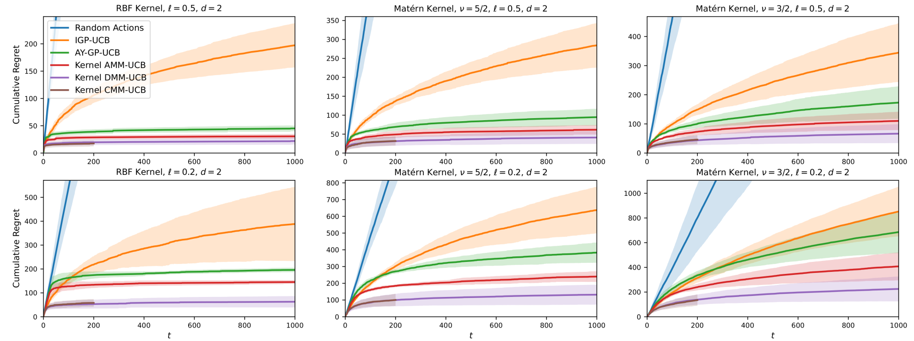
Figure 5: Cumulative regret of our KernelUCB-style algorithms as well as AY-GP-UCB, IGP-UCB and a random baseline over $T=1000$ rounds for $d=2$ and various kernels (columns) and length scales (rows). We show the mean $\pm$ standard deviation over 10 repetitions.

In Fig. 5, we observe that our Kernel CMM-UCB and Kernel DMM-UCB algorithms achieve the lowest cumulative regret, followed by Kernel AMM-UCB and the AY-GP-UCB and IGP-UCB. All methods performed noticeably better with 2-dimensional action sets than with 3-dimensional action sets (see Fig. 2).

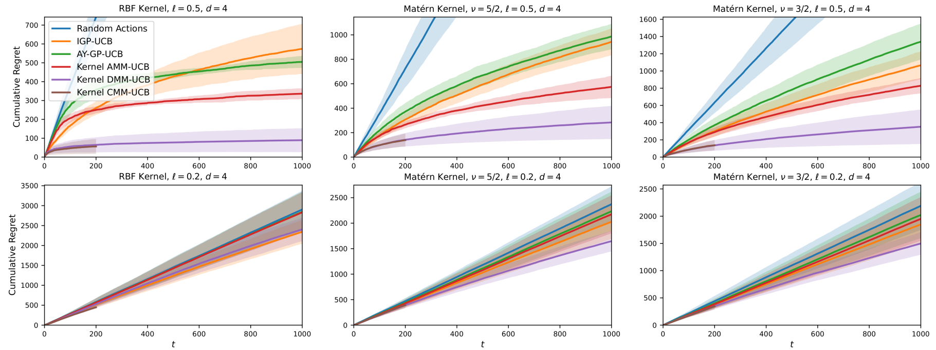
Figure 6: Cumulative regret of our KernelUCB-style algorithms as well as AY-GP-UCB, IGP-UCB and a random baseline over $T=1000$ rounds for $d=4$ and various kernels (columns) and length scales (rows). We show the mean $\pm$ standard deviation over 10 repetitions.

In Fig. 6, we observe a similar drop in the performance of all methods when moving up to 4-dimensional action sets. In the top row of Fig. 6, in which the kernel length-scale is $\ell=0.5$, we observe that each method still achieves much lower cumulative regret than the random baseline, and Kernel CMM-UCB and Kernel DMM-UCB algorithms still achieve the lower cumulative regret. However, in bottom row of Fig. 6, we see that no method performs much better than the random baseline.

F.3 Loose Upper Bounds on $B$ and $\sigma$

To run each kernel bandit algorithm, we only need to know upper bounds on the sub-Gaussian parameter $\sigma$ and the bound $B$ on the RKHS norm of the reward function $f^{*}$. We now investigate what happens when the known bounds on one or both of these quantities are loose.

We run each algorithm in the same synthetic kernel bandit problem as described in Sec. 7, where the kernel is a Matérn kernel with smoothness $\nu=5/2$ and length-scale $\ell=0.5$, and the actions are 3-dimensional vectors in $[0,1]^{3}$. As before, the noise variable are $\sigma$-sub-Gaussian with $\sigma=0.1$ and $\left\|f^{*}\right\|=10$. We run each algorithm with all four pairs of values of $(\sigma,B)$, where $\sigma\in\{0.1,0.2\}$ and $B\in\{10,20\}$.

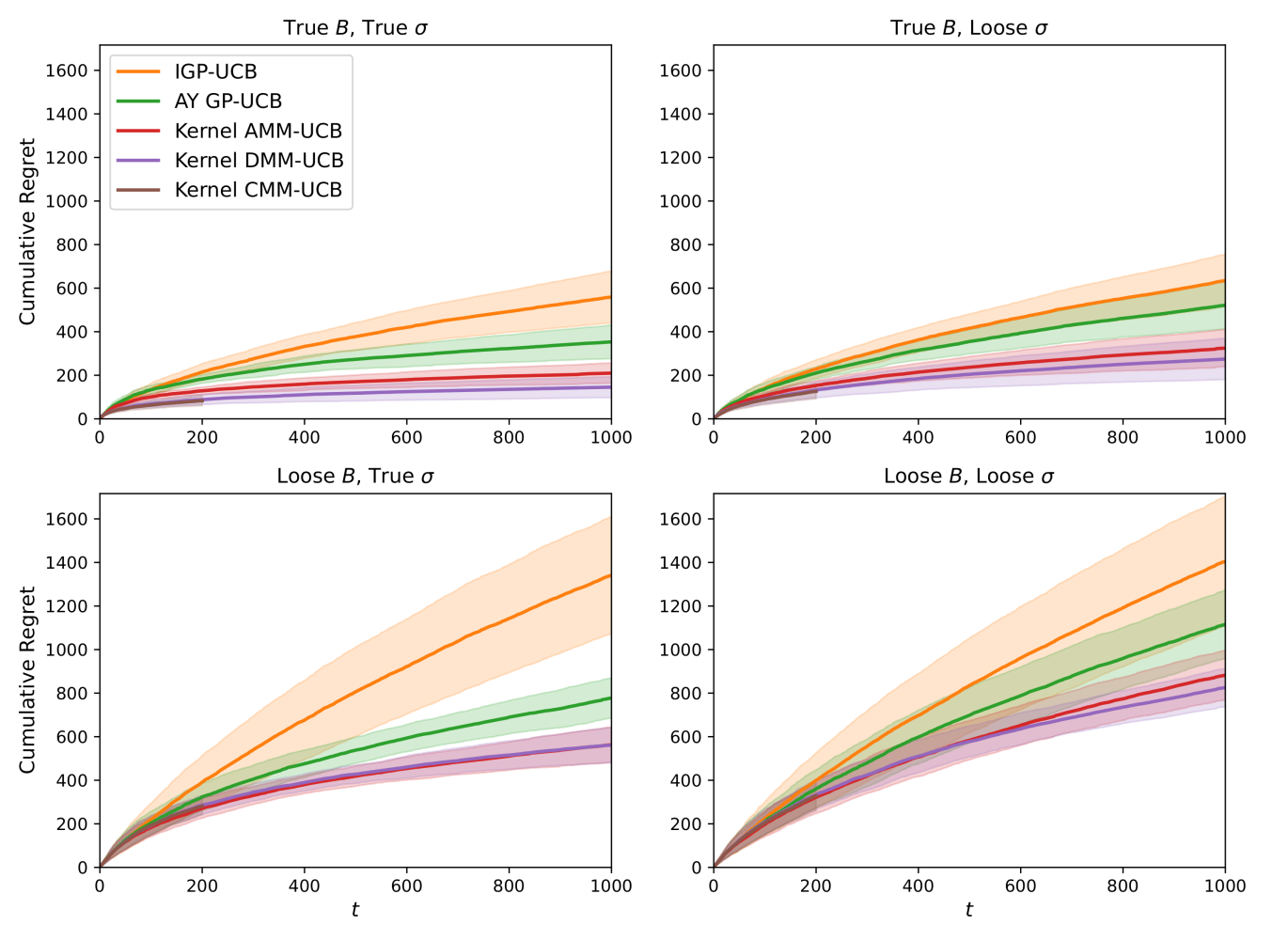
Figure 7: Cumulative regret of our kernel UCB-style algorithms as well as AY-GP-UCB, IGP-UCB and a random baseline after $T=1000$ rounds for various kernels (columns) and length scales (rows). The action sets are subsets of $[0,1]^{4}$. We show the mean $\pm$ standard deviation over 10 repetitions.

Fig. 7 shows the cumulative regret of each method and with each combination of correct or loose $\sigma$ and $B$. We observe that using a loose upper bound on $\sigma$ has a relatively small effect on each method, whereas a loose bound on $B$ can cause the cumulative regret of each method to grow considerably.

References

• Abbasi-Yadkori (2012) Abbasi-Yadkori, Y. Online learning for linearly parametrized control problems. PhD thesis, University of Alberta, 2012.
• Abbasi-Yadkori etΒ al. (2011) Abbasi-Yadkori, Y., PΓ‘l, D., and SzepesvΓ‘ri, C. Improved algorithms for linear stochastic bandits. Advances in neural information processing systems, 24, 2011.
• Abbasi-Yadkori etΒ al. (2012) Abbasi-Yadkori, Y., Pal, D., and Szepesvari, C. Online-to-confidence-set conversions and application to sparse stochastic bandits. In Artificial Intelligence and Statistics, pp.Β  1–9. PMLR, 2012.
• Agrawal etΒ al. (2019) Agrawal, A., Amos, B., Barratt, S., Boyd, S., Diamond, S., and Kolter, J.Β Z. Differentiable convex optimization layers. Advances in neural information processing systems, 32, 2019.
• Auer (2002) Auer, P. Using confidence bounds for exploitation-exploration trade-offs. Journal of Machine Learning Research, 3(Nov):397–422, 2002.
• Berkenkamp etΒ al. (2017) Berkenkamp, F., Turchetta, M., Schoellig, A., and Krause, A. Safe model-based reinforcement learning with stability guarantees. Advances in neural information processing systems, 30, 2017.
• Blondel etΒ al. (2022) Blondel, M., Berthet, Q., Cuturi, M., Frostig, R., Hoyer, S., Llinares-LΓ³pez, F., Pedregosa, F., and Vert, J.-P. Efficient and modular implicit differentiation. Advances in neural information processing systems, 35:5230–5242, 2022.
• Cesa-Bianchi & Lugosi (2006) Cesa-Bianchi, N. and Lugosi, G. Prediction, learning, and games. Cambridge university press, 2006.
• Chowdhury & Gopalan (2017) Chowdhury, S.Β R. and Gopalan, A. On kernelized multi-armed bandits. In International Conference on Machine Learning, pp.Β 844–853. PMLR, 2017.
• deΒ la PeΓ±a etΒ al. (2004) deΒ la PeΓ±a, V.Β H., Klass, M.Β J., and LeungΒ Lai, T. Self-normalized processes: exponential inequalities, moment bounds and iterated logarithm laws. Annals of Probability, 32:1902–1933, 2004.
• deΒ la PeΓ±a etΒ al. (2009) deΒ la PeΓ±a, V.Β H., Lai, T.Β L., and Shao, Q.-M. Self-normalized processes: Limit theory and Statistical Applications. Springer, 2009.
• Diamond & Boyd (2016) Diamond, S. and Boyd, S. CVXPY: A Python-embedded modeling language for convex optimization. Journal of Machine Learning Research, 17(83):1–5, 2016.
• Durand etΒ al. (2018) Durand, A., Maillard, O.-A., and Pineau, J. Streaming kernel regression with provably adaptive mean, variance, and regularization. The Journal of Machine Learning Research, 19(1):650–683, 2018.
• Emmenegger etΒ al. (2023) Emmenegger, N., Mutnα»³, M., and Krause, A. Likelihood ratio confidence sets for sequential decision making. In Advances in Neural Information Processing Systems (NeurIPS), 2023.
• Flynn etΒ al. (2023) Flynn, H., Reeb, D., Kandemir, M., and Peters, J. Improved algorithms for stochastic linear bandits using tail bounds for martingale mixtures. In Advances in Neural Information Processing Systems (NeurIPS), 2023.
• Jamieson etΒ al. (2014) Jamieson, K., Malloy, M., Nowak, R., and Bubeck, S. lil’ucb: An optimal exploration algorithm for multi-armed bandits. In Conference on Learning Theory, pp.Β  423–439. PMLR, 2014.
• Janz etΒ al. (2020) Janz, D., Burt, D., and GonzΓ‘lez, J. Bandit optimisation of functions in the matΓ©rn kernel rkhs. In International Conference on Artificial Intelligence and Statistics, pp.Β  2486–2495. PMLR, 2020.
• Kakade etΒ al. (2020) Kakade, S., Krishnamurthy, A., Lowrey, K., Ohnishi, M., and Sun, W. Information theoretic regret bounds for online nonlinear control. Advances in Neural Information Processing Systems, 33:15312–15325, 2020.
• Kimeldorf & Wahba (1971) Kimeldorf, G. and Wahba, G. Some results on tchebycheffian spline functions. Journal of mathematical analysis and applications, 33(1):82–95, 1971.
• Lattimore (2023) Lattimore, T. A lower bound for linear and kernel regression with adaptive covariates. In The Thirty Sixth Annual Conference on Learning Theory, pp.Β 2095–2113. PMLR, 2023.
• Lattimore & SzepesvΓ‘ri (2020) Lattimore, T. and SzepesvΓ‘ri, C. Bandit algorithms. Cambridge University Press, 2020.
• Li & Scarlett (2022) Li, Z. and Scarlett, J. Gaussian process bandit optimization with few batches. In International Conference on Artificial Intelligence and Statistics, pp.Β  92–107. PMLR, 2022.
• Liu & Su (2022) Liu, S. and Su, H. Provably efficient kernelized Q-learning. arXiv preprint arXiv:2204.10349, 2022.
• Look etΒ al. (2020) Look, A., Doneva, S., Kandemir, M., Gemulla, R., and Peters, J. Differentiable implicit layers. In NeurIPS ML for Engineering Workshop, 2020.
• Neiswanger & Ramdas (2021) Neiswanger, W. and Ramdas, A. Uncertainty quantification using martingales for misspecified Gaussian processes. In Algorithmic Learning Theory, pp.Β  963–982. PMLR, 2021.
• Russo & VanΒ Roy (2013) Russo, D. and VanΒ Roy, B. Eluder dimension and the sample complexity of optimistic exploration. Advances in Neural Information Processing Systems, 26, 2013.
• SchΓΆlkopf etΒ al. (2001) SchΓΆlkopf, B., Herbrich, R., and Smola, A.Β J. A generalized representer theorem. In International conference on computational learning theory, pp.Β  416–426. Springer, 2001.
• Srinivas etΒ al. (2010) Srinivas, N., Krause, A., Kakade, S., and Seeger, M. Gaussian process optimization in the bandit setting: No regret and experimental design. In Proc. International Conference on Machine Learning (ICML), 2010.
• Sui etΒ al. (2015) Sui, Y., Gotovos, A., Burdick, J., and Krause, A. Safe exploration for optimization with gaussian processes. In International conference on machine learning, pp.Β 997–1005. PMLR, 2015.
• Sutton & Barto (2018) Sutton, R.Β S. and Barto, A.Β G. Reinforcement learning: An introduction. MIT press, 2018.
• Vakili & Olkhovskaya (2023) Vakili, S. and Olkhovskaya, J. Kernelized reinforcement learning with order optimal regret bounds. In Advances in Neural Information Processing Systems (NeurIPS), 2023.
• Vakili etΒ al. (2021) Vakili, S., Khezeli, K., and Picheny, V. On information gain and regret bounds in gaussian process bandits. In International Conference on Artificial Intelligence and Statistics, pp.Β  82–90. PMLR, 2021.
• Valko etΒ al. (2013) Valko, M., Korda, N., Munos, R., Flaounas, I., and Cristianini, N. Finite-Time Analysis of Kernelised Contextual Bandits. In Uncertainty in Artificial Intelligence, 2013.
• Ville (1939) Ville, J. Etude critique de la notion de collectif. Bull. Amer. Math. Soc, 45(11):824, 1939.
• Whitehouse etΒ al. (2023) Whitehouse, J., Wu, Z.Β S., and Ramdas, A. On the sublinear regret of gp-ucb. Advances in Neural Information Processing Systems, 2023.
• Yang etΒ al. (2020) Yang, Z., Jin, C., Wang, Z., Wang, M., and Jordan, M.Β I. On function approximation in reinforcement learning: optimism in the face of large state spaces. In Proceedings of the 34th International Conference on Neural Information Processing Systems, pp.Β  13903–13916, 2020.
• Zhang (2006) Zhang, F. The Schur complement and its applications, volumeΒ 4. Springer Science & Business Media, 2006.