Revisiting the Dirac Nature of Neutrinos

Abstract

Amid the uncertainty regarding the fundamental nature of neutrinos, we adhere to the Dirac one, and construct a model in the light of $\Delta(27)$ symmetry. The model is enriched by an additional $Z_{10}$ symmetry, to eliminate the possibility of the Majorana mass terms. The neutrino mass matrix exhibits four texture zeroes, and the associated mixing scheme aligns with the experimental data, notably controlled by a single parameter. In addition, the model emphasizes on the standard parametrization of the lepton mixing matrix, which is crucial in the light of model building and neutrino physics experiments.

I Introduction

The neutrinos are an essential part of the Standard Model(SM) of particle physics. According to the SM, neutrinos are massless particles. However, a quantum mechanical phenomenon called Neutrino Oscillation, originally proposed by Bruno Pontecorvo in 1957 [1], suggests that the three mass eigenstates of neutrinos ($\nu_{i=1,2,3}$) mix together to generate the three flavour neutrino states ($\nu_{l=e,\mu,\tau}$). In recent past, observations from various experiments [2, 3, 4] confirmed the occurrence of neutrino oscillation, and it was seen that, for the oscillation to occur, the neutrinos should have non zero and non-degenerate masses. Hence, the SM has two primary shortcomings: it cannot fully explain the reason why neutrinos of different flavours mix together peculiarly, and it cannot account for the extremely small masses of neutrinos. The search for answers to these questions has taken us to the realm of neutrino mass matrix textures. The term “neutrino mass matrix” refers to a mathematical structure which contains the information of the neutrino masses and mixing, and the term “neutrino mass matrix texture” refers to certain patterns among the elements of the neutrino mass matrix. These patterns serve to reduce the number of free parameters in the mass matrix and help to draw important correlations among the observable quantities. To understand the neutrino mass matrix textures, researchers have primarily investigated the idea that neutrinos are their own antiparticles, known as Majorana neutrinos. This assumption is motivated by the fact that, for the Majorana nature, the equations describing neutrino masses ($\sim\bar{\nu_{L}}\nu_{R}+h.c$) become simpler because they can be constructed solely from left-handed neutrinos, represented as $\sim\bar{\nu_{L}}\nu^{c}_{L}+h.c$. Majorana nature allows us to equate $\nu_{R}$ (right-handed neutrinos) with $\nu^{c}_{L}$ (charge conjugate of the left-handed neutrino), eliminating the need for an additional right-handed component. The Majorana mass term ($\sim\bar{\nu_{L}}\nu^{c}_{L}+h.c$), is a lepton number violating term, it violates the lepton number by two units. In the SM, this term is applicable only to neutrinos, as they are electrically neutral. However, it is to be emphasized that the Majorana nature of neutrinos is subject to experimental verification. In this light, experiments on neutrino less double-beta ($0\nu\beta\beta$) decay is considered to be the most promising one (for a detailed review, refer to [5, 6, 7]). Although attempts to identify $0\nu\beta\beta$ decay have been going on for almost a century, there is, so far no evidence to support it [7]. This leaves ample room for the discussions related to the Dirac nature. In the present work, we adhere to the Dirac nature of the neutrinos.

The plan of our work is as follows: In Section II, we discuss the framework on which the model is built. In addition, we also discuss the standard parametrization of the lepton mixing matrix predicted from our model. In Section III, we shed light on the numerical analysis and findings of our study. Finally, in Section IV, we highlight the summary and discussions of the present study.

II Framework

We minimally extend the field content of the SM with right handed neutrinos ($\nu_{R}$), and three additional complex scalar fields, namely, $\psi,\phi$ and $\kappa$. Our model is grounded in the framework of $\Delta(27)$ symmetry. The discrete symmetry group $\Delta(27)$ [8, 9, 10, 11, 12, 13, 14] has 11 irreducible representations, namely, one triplet ($3$), one anti-triplet  ($\bar{3}$) and nine singlet ($1_{p,q}$) representations, where $p$ and $q$ are integers, and can take values from 0 to 2. We further enrich the model with the $Z_{10}$ group [15, 16], representing a modulus symmetry that operates within the integers modulo 10. A brief discussion about the product rules associated with $\Delta(27)$ symmetry and $Z_{10}$ is shown in the Appendix VI.

II.1 Model

The transformation properties of the field contents in our present model are tabulated in Table 1.

Fields	$\bar{D}_{l_{L}}$	$l_{R}$	$H$	$\nu_{R}$	$\psi$	$\phi$	$\kappa$
$\Delta(27)$	3	$(1_{00},1_{22},1_{11})$	$1_{00}$	3	$\bar{3}$	3	3
$Z_{10}$	1	5	0	6	4	3	2
$SU(2)_{L}$	2	1	2	1	1	1	1

Table 1: The transformation properties of the field contents under $\Delta(27)\times Z_{10}\times SU(2)_{L}$

The Yukawa Lagrangian invariant under $\Delta(27)\times Z_{10}\times SU(2)_{L}$ symmetry is presented as shown,

$$-\mathcal{L}_{Y} = \frac{y_{e}}{\Lambda}(\bar{D}_{l_{L}}\psi)\,H\,e_{R}+\,\frac{y_{\mu}}{\Lambda}(\bar{D}_{l_{L}}\psi)\,H\,\mu_{R}+\,\frac{y_{\tau}}{\Lambda}(\bar{D}_{l_{L}}\psi)\,H\,\tau_{R}+\frac{y_{s}}{\Lambda}\,(\bar{D}_{l_{L}}\phi)\,\tilde{H}\,\nu_{R}+\frac{y_{a}}{\Lambda}\,(\bar{D}_{l_{L}}\phi)$$ (1)

$$\,\tilde{H}\,\nu_{R}+\frac{y_{d}}{\Lambda}\,(\bar{D}_{l_{L}}\nu_{R})\,\tilde{H}\,\kappa\,.$$

From Table 1, we observe that $\nu_{R}$, $\phi$, and $\kappa$ are singlets and triplets under $SU(2)_{L}$ and $\Delta(27)$, respectively. Therefore, the $Z_{10}$ group helps distinguish these singlets from each other, and it forbids the Majorana mass terms at the tree level. In addition, the $Z_{10}$ group enforces the complex scalar fields $\psi$ and $\phi$ to couple to the charged leptons and right handed neutrinos respectively, and restricts the next to leading order (NLO) corrections in the Yukawa Lagrangian ($\mathcal{L}_{Y}$).

We assume that the scalar fields develop the vacuum expectation value (VEV) in the following directions: $\langle\psi\rangle=v_{\psi}(1,1,1)$, $\langle\phi\rangle=v_{\phi}(0,1,0)$, $\langle\kappa\rangle=v_{\kappa}(1,1,1)$ and $\langle H\rangle=v_{h}$. A detailed discussion on the scalar potential for the said alignments is shown in the Appendix VII. The said alignments are necessary to generate the correct mixing pattern and it keeps the charged lepton mass matrix ($M_{L}$) non diagonal. The form of $M_{L}$ is shown below,

$$M_{L}=\frac{v_{\psi}v_{h}}{\Lambda}\begin{bmatrix}y_{e}&y_{\mu}&y_{\tau}\\ y_{e}&\omega^{2}\,y_{\mu}&\omega\,y_{\tau}\\ y_{e}&\omega\,y_{\mu}&\omega^{2}\,y_{\tau}\\ \end{bmatrix},$$ (2)

where,

$$\omega=e^{2\pi i/3}.$$ (3)

The four texture zero [17, 18, 19, 20] Dirac neutrino mass matrix($M_{\nu}$) appears as shown below,

$$M_{\nu}=\begin{bmatrix}\frac{v_{h}y_{d}v_{k}}{\Lambda}&0&\frac{v_{h}(y_{s}+y_{a})v_{\phi}}{\Lambda}\\ 0&\frac{v_{h}y_{d}v_{k}}{\Lambda}&0\\ \frac{v_{h}(y_{s}-y_{a})v_{\phi}}{\Lambda}&0&\frac{v_{h}y_{d}v_{k}}{\Lambda}\\ \end{bmatrix},$$ (4)

Such a similar form of the neutrino mass matrix was achieved in the Ref. [21], using the neutrinophilic two Higgs doublet model [22, 23] and in Refs. [24, 25], using the Dirac seesaw mechanism. However, our approach differs from those mentioned. We do not consider the Dirac seesaw mechanism for neutrino mass generation and our field content is minimal. Unlike $A_{4}$ symmetry, we have used the framework of $\Delta(27)$ symmetry. The presence of the additional anti-triplet ($\bar{3}$) representation in the $\Delta(27)$ symmetry, helps with a greater flexibility of tuning the neutrino mass matrix with a minimal field content. It is worth mentioning that in the ref [21] and in literature [23, 26, 27], the $U(1)$ group is widely employed to forbid the Majorana mass term. However, in our approach, we have opted for the $Z_{10}$ group instead. For the sake of simplicity, we redefine the elements of $M_{\nu}$ such that, $v_{h}(y_{s}-y_{a})v_{\phi}/\Lambda=r_{1}e^{i\gamma_{1}},v_{h}(y_{s}+y_{a})v_{\phi}/\Lambda=r_{2}e^{i\gamma_{2}}$ and $v_{h}y_{d}v_{k}/\Lambda=r_{3}e^{i\gamma_{3}}$. To understand the physics related to the neutrino mass matrix $M_{\nu}$, we define a hermitian matrix:

$$H=M_{\nu}M^{\dagger}_{\nu}=\begin{bmatrix}r^{2}_{2}+r^{2}_{3}&0&r_{1}r_{3}e^{i(\gamma_{3}-\gamma_{1})}+r_{2}r_{3}e^{i(\gamma_{2}-\gamma_{3})}\\ 0&r^{2}_{3}&0\\ r_{1}r_{3}e^{-i(\gamma_{3}-\gamma_{1})}+r_{2}r_{3}e^{-i(\gamma_{2}-\gamma_{3})}&0&r^{2}_{1}+r^{2}_{3}\\ \end{bmatrix},$$ (5)

which can be diagonalised with the help of a unitary matrix,, $U_{\nu}$ in the following way: $U_{\nu}^{\dagger}HU_{\nu}=diag\,(m_{1}^{2},m_{2}^{2},m_{3}^{2})$. Here, $m_{1},m_{2}$ and $m_{3}$ are the three neutrino mass eigenvalues. The unitarity condition condition enforces $r_{1}=r_{2}=r$, and the mixing matrix, $U_{\nu}$ takes the following form,

$$U_{\nu}=\frac{1}{\sqrt{2}}\begin{bmatrix}-e^{i\rho}&0&e^{i\rho}\\ 0&\sqrt{2}&0\\ 1&0&1\\ \end{bmatrix},$$ (6)

where,

$$\rho=-\tan^{-1}\frac{\sin(\gamma_{1}-\gamma_{3})-\sin(\gamma_{2}-\gamma_{3})}{\cos(\gamma_{1}-\gamma_{3})+\cos(\gamma_{2}-\gamma_{3})}.$$ (7)

The neutrino mass eigenvalues are obtained as:

$$m_{1} = \sqrt{r^{2}+r_{3}^{2}-r\,r_{3}(2+2x)^{1/2}},$$ (8)

$$m_{2} = r_{3},$$ (9)

$$m_{3} = \sqrt{r^{2}+r_{3}^{2}+r\,r_{3}(2+2x)^{1/2}},$$ (10)

where $x=\cos\,(\gamma_{1}+\gamma_{2}-2\gamma_{3})$. It is noteworthy that the relation, $\Delta m^{2}_{31}=2rr_{3}\sqrt{2\,(1+x)}$, is always greater than zero, as $r>0$ and $r_{3}>0$. Hence, our model is true only for the normal ordering of neutrino masses.

The charged lepton mass matrix ($M_{L}$), can be diagonalized in the following way:

$$U_{L}^{\dagger}M_{L}U_{R}=\begin{bmatrix}\sqrt{3}v_{h}v_{\psi}y_{e}/\Lambda&0&0\\ 0&\sqrt{3}v_{h}v_{\psi}y_{\mu}/\Lambda&0\\ 0&0&\sqrt{3}v_{h}v_{\psi}y_{\tau}/\Lambda\\ \end{bmatrix},$$ (11)

where, $U_{L}$ and $U_{R}$ are left handed and right handed charged lepton diagonalising matrices respectively. The form of $U_{L}$ and $U_{R}$ is shown below,

$$U_{L}=\frac{-1}{\sqrt{3}}\begin{bmatrix}1&1&1\\ 1&\omega^{2}&\omega\\ 1&\omega&\omega^{2}\\ \end{bmatrix},\quad U_{R}=\begin{bmatrix}-1&0&0\\ 0&-1&0\\ 0&0&-1\\ \end{bmatrix}.$$ (12)

The final lepton mixing matrix of our model is given by:

$$U=U_{L}^{\dagger}.U_{\nu}=\left[\begin{array}[]{ccc}-\frac{-1+e^{i\rho}}{\sqrt{6}}&\frac{1}{\sqrt{3}}&\frac{1+e^{i\rho}}{\sqrt{6}}\\ \frac{\omega^{2}-e^{i\rho}}{\sqrt{6}}&\frac{\omega}{\sqrt{3}}&\frac{\omega^{2}+e^{i\rho}}{\sqrt{6}}\\ \frac{\omega-e^{i\rho}}{\sqrt{6}}&\frac{\omega^{2}}{\sqrt{3}}&\frac{\omega+e^{i\rho}}{\sqrt{6}}\\ \end{array}\right].$$ (16)

Needless to mention that in the above equation, $\rho$ is the only free parameter. Before we try to fetch the information of the observational oscillation parameters from $U$, we need to ensure that $U$ is represented as per standard or particle data group(PDG) parametrization [28]. This is to be highlighted that most often, the model builders overlook this important and necessary step  [21, 29, 24, 25].

II.2 Standard Parametrisation

A general $3\times 3$ unitary matrix carries nine free parameters and the lepton mixing matrix is no exception. However, the oscillation experiments deal only with four parameters out of nine. These are three mixing angles: solar angle ($\theta_{12}$), reactor angle ($\theta_{13}$), and atmospheric angle ($\theta_{23}$) as well as the Dirac Charge Parity (CP) violating phase ($\delta$). The remaining parameters remain unobserved or unphysical. To ensure that the predictions are correct, we need to transform $U$ to $U_{std}$ following the transformation as shown below.

$$U_{std}=P^{*}_{\chi}.U.P^{*}_{\xi},$$ (17)

where, the matrices $P_{\chi}$ and $P_{\xi}$ carry the five unphysical parameters: $\chi_{1}$, $\chi_{2}$, $\chi_{3}$, $\xi_{1}$ and $\xi_{2}$, and these matrices are presented as shown: $P_{\chi}=diag(e^{i\chi_{1}},e^{i\chi_{2}},e^{i\chi_{3}})$ and $P_{\xi}=diag(e^{i\xi_{1}},e^{i\xi_{2}},1)$. So that the $U_{std}$ appears as per PDG parametrization, as shown below.

$$U_{std} = \left[\begin{array}[]{ccc}c_{12}c_{13}&c_{13}s_{12}&e^{-i\delta}s_{13}\\ -c_{23}s_{12}-e^{i\delta}c_{12}s_{13}s_{23}&c_{12}c_{23}-e^{i\delta}s_{12}s_{13}s_{23}&c_{13}s_{23}\\ s_{12}s_{23}-e^{i\delta}c_{12}c_{23}s_{13}&-c_{12}s_{23}-e^{i\delta}c_{23}s_{12}s_{13}&c_{13}c_{23}\\ \end{array}\right]$$ (21)

where, $s_{ij}=\sin\theta_{ij}$ and $c_{ij}=\cos\theta_{ij}$.

After this transformation, the four observational parameters are predicted as shown in the following,

$$\sin^{2}{\theta_{12}} = \frac{1}{2-\cos(\rho)},$$ (22)

$$\sin^{2}{\theta_{13}} = \frac{1+\cos(\rho)}{3},$$ (23)

$$\sin^{2}{\theta_{23}} = \frac{\sqrt{3}\sin(\rho)+\cos(\rho)-2}{2\cos(\rho)-4},$$ (24)

$$\delta = \chi_{1}-\frac{\rho}{2}.$$ (25)

It is interesting to note the three mixing angles are dictated by a single parameter, $\rho$, in contrast to [21, 24, 25]. It seems that in the expression of Dirac CP phase, $\delta$, in Eq. (25), $\chi_{1}$ is an independent parameter. However, $\chi_{1}$ along with other four unphysical parameters can be worked out by solving the following five transcendental equations,

$$2\sqrt{1-\cos(\rho)}\left(\sqrt{3}\sin\left(\xi_{2}+\chi_{2}\right)+3\cos\left(\xi_{2}+\chi_{2}\right)\right)$$

$$-\sqrt{6}\left(\sin\left(\xi_{1}+\chi_{2}\right)-2\sin\left(\rho-\xi_{1}-\chi_{2}\right)\right)$$

$$+3\sqrt{2}\cos\left(\xi_{1}+\chi_{2}\right)= 0,$$ (26)

$$\sin\left(\xi_{2}+\chi_{1}\right)= 0,$$ (27)

$$\sin\left(\rho-\xi_{1}-\chi_{1}\right)+\sin\left(\xi_{1}+\chi_{1}\right)= 0,$$ (28)

$$3\cos\left(\chi_{2}\right)-\sqrt{3}\left(2\sin\left(\rho-\chi_{2}\right)+\sin\left(\chi_{2}\right)\right)= 0,$$ (29)

$$\sqrt{3}\left(2\sin\left(\rho-\chi_{3}\right)+\sin\left(\chi_{3}\right)\right)+3\cos\left(\chi_{3}\right)= 0,$$ (30)

which are obtained from the five standard parametrization conditions. This is to be noted that $\rho$ is the only free parameter appearing in Eq. (II.2) and Eqs. (29)-(30). Hence, we understand that $\chi_{1}$ appearing in Eq. (25) is not independent, rather relies on $\rho$. Therefore, $\delta$ along with the three mixing angles are basically guided by $\rho$ itself.

In the next section we will study the predictions of the present model for a wide range of data points.

III Numerical Analysis and Results

We, numerically solve the Eqs. (II.2) -  (30) simultaneously in order to generate sufficiently large number of data points for the unphysical phases $\chi_{1}$, $\chi_{2}$, $\chi_{3}$, $\xi_{1}$ and $\xi_{2}$. The maximum and minimum values of the said phases and the parameter $\rho$ are tabulated in Table 2. We graphically represent these phases in Figures 1, 1 and 1. Though the measurement of the unphysical phases are not motivated in the experiments, yet from the model building point of view, this information could be significant.

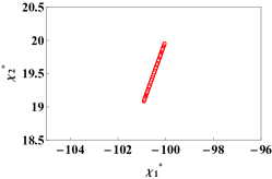
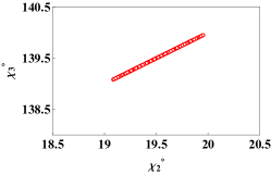
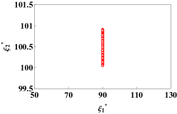
Figure 1: The plots for the unphysical phases (a) Plots the relationship between $\chi_{1}$ and $\chi_{2}$ (b) Highlights the plot for $\chi_{2}$ vs $\chi_{3}$ and (c) Represents the plot between $\xi_{1}$ and $\xi_{2}$

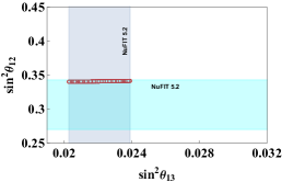
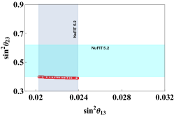
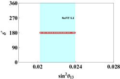
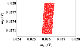
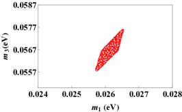
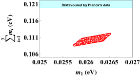
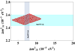
Figure 2: The plots for the observable parameters are shown: (a) Plots the relationship between the free parameters $\sin^{2}{\theta_{13}}$ and $\sin^{2}{\theta_{12}}$ (b) Highlights the plot for $\sin^{2}{\theta_{23}}$ vs $\sin^{2}{\theta_{13}}$  (c) Shows the plot depicting the relationship between $\sin^{2}{\theta_{13}}$ and $\delta$ (d) shows the plot for $m_{2}$ vs $m_{1}$  (e) Represents the plot between $m_{3}$ and $m_{1}$ (f) Highlights the plot for $\sum{m_{i}}$ vs the lightest neutrino mass, $m_{1}$ and (g) Represents the plot for the $\Delta m^{2}_{31}$ vs $\Delta m^{2}_{21}$.

Parameters	Minimum Value	Maximum Value
$\rho/^{\circ}$	158.1730	159.9030
$\chi_{1}/^{\circ}$	-100.9130	-100.0490
$\chi_{2}/^{\circ}$	19.0860	19.9513
$\chi_{3}/^{\circ}$	139.0870	139.9510
$\xi_{1}/^{\circ}$	90	90
$\xi_{2}/^{\circ}$	100.0490	100.9130

Table 2: Represents the maximum and minimum values for the unphysical phases and the parameter $\rho$

It is interesting to note that for the $3\sigma$ range of $\sin^{2}{\theta_{13}}$, the observables $\sin^{2}{\theta_{12}}$ and $\sin^{2}{\theta_{23}}$ are predicted at the extreme ends of the experimental $3\sigma$ range [30, 31]. Specifically, $\sin^{2}{\theta_{23}}$, lies in the lower octant. The Dirac CP phase $\delta$ is found to be $180^{\circ}$. It is to be highlighted that our model rules out the possibility of the inverted ordering of neutrino masses. Hence, in the light of the normal ordering, the predicted upper bound on the sum of the neutrino masses is consistent with the cosmological data [32]. The upper bound on the three neutrino mass eigenvalues, $m_{1}$, $m_{2}$ and $m_{3}$ are $0.0265\,eV$, $0.0279\,eV$ and $0.0575\,eV$ respectively. For this analysis, the input model parameters are tuned within certain numerical bounds: $0.0340\,eV<r<0.0350\,eV$, $0.0270\,eV<r_{3}<0.0280\,eV$ and $-0.1125<x<-0.1120$. We show the maximum and minimum values of the predicted parameters in Table (3). The graphical representations of the said predictions are shown in Figures 2, 2, 2, 2, 2, 2 and 2.

Predictions	Minimum Value	Maximum Value
$\sin^{2}{\theta_{12}}$	0.3402	0.3414
$\sin^{2}{\theta_{13}}$	0.0203	0.0238
$\sin^{2}{\theta_{23}}$	0.3900	0.4000
$\delta/^{\circ}$	180	180
$\Delta m^{2}_{21}$/$eV^{2}$	0.000035	0.00011
$\Delta m^{2}_{31}$/$eV^{2}$	0.00244	0.00260
$m_{1}$/$eV$	0.0257	0.0265
$m_{2}$/$eV$	0.0270	0.0279
$m_{3}$/$eV$	0.0558	0.0575
$\sum{m_{i}}$/$eV$	0.1085	0.1120

Table 3: Represents the approximate maximum and minimum values for the observable parameters

IV Summary and Discussions

In the present study, we have adopted the Dirac neutrino model because of the continuing uncertainty about the fundamental nature of neutrinos. In this model, we have constructed a neutrino mass matrix in the framework of $\Delta(27)$ symmetry. The model contains only a few flavons, and therefore it is minimal. We have enhanced the framework by an additional symmetry, $Z_{10}$, which restricts the NLO terms and forbids the possible Majorana mass terms. The model is predictive, and a single guiding parameter, $\rho$, spans the three mixing angles and the Dirac CP phase. The observable $\sin^{2}{\theta_{13}}$, lies within the experimental bound, in addition, $\sin^{2}{\theta_{12}}$ and $\sin^{2}{\theta_{23}}$ are found to be at the extreme ends of the experimental $3\sigma$ range. The Dirac CP phase $\delta$ is predicted as $180^{\circ}$. Our model is consistent with the normal ordering of neutrino masses and it predicts the three neutrino mass eigenvalues, $m_{1}$, $m_{2}$ and $m_{3}$ to be in the upper bounds of $0.0265\,eV$, $0.0279\,eV$, and $0.0575\,eV$ respectively. In addition, the upper bound on the sum of the three neutrino masses is found to be $\sim 0.1120\,eV$, which is in good agreement with the Planck’s cosmological data. Furthermore, we have emphasized the standard parametrization of the lepton mixing matrix, which is often overlooked by model builders. This parametrization is important from model model-building point of view because a general unitary matrix contains nine parameters, out of which five are unphysical in the context of neutrino physics experiments. Therefore, we have taken special care to isolate these phases from our lepton mixing matrix to ensure an accurate mixing scheme.

V Acknowledgement

The Research work of MD is supported by the Council of Scientific and Industrial Research (CSIR), Government of India through a NET Junior Research Fellowship vide grant No. 09/0059(15346)/2022-EMR-I.

VI Appendix A

$\Delta(27)$ group

The multiplication rules under the $\Delta(27)$ group is given below,

$$3\otimes 3 = \bar{3}_{s_{1}}\oplus\bar{3}_{s_{2}}\oplus\bar{3}_{a},$$

$$\bar{3}\otimes\bar{3} = 3_{s_{1}}\oplus 3_{s_{2}}\oplus 3_{a},$$

$$3\otimes\bar{3} = \sum_{r=0}^{2}1_{r,0}\oplus\sum_{r=0}^{2}1_{r,1}\oplus\sum_{r=0}^{2}1_{r,2},$$

$$1_{p,q}\otimes 1_{p^{\prime},q^{\prime}} = 1_{(p+p^{\prime})\,\text{mod}\,3,\,(q+q^{\prime})\,\text{mod}\,3}.$$ (31)

If $(a_{1},a_{2},a_{3})$ and $(b_{1},b_{2},b_{3})$ are two triplets under $\Delta(27)$ then,

$$(3\otimes 3)_{\bar{3}_{s_{1}}} = (a_{1}b_{1},a_{2}b_{2},a_{3}b_{3}),$$

$$(3\otimes 3)_{\bar{3}_{s_{2}}} = \frac{1}{2}(a_{2}b_{3}+a_{3}b_{2},a_{3}b_{1}+a_{1}b_{3},a_{1}b_{2}+a_{2}b_{1}),$$

$$(3\otimes 3)_{\bar{3}_{a}} = \frac{1}{2}(a_{2}b_{3}-a_{3}b_{2},a_{3}b_{1}-a_{1}b_{3},a_{1}b_{2}-a_{2}b_{1}),$$

$$(3\otimes\bar{3})_{1_{r,0}} = a_{1}b_{1}+\omega^{2r}a_{2}b_{2}+\omega^{r}a_{3}b_{3},$$

$$(3\otimes\bar{3})_{1_{r,1}} = a_{1}b_{2}+\omega^{2r}a_{2}b_{3}+\omega^{r}a_{3}b_{1},$$

$$(3\otimes\bar{3})_{1_{r,2}} = a_{1}b_{3}+\omega^{2r}a_{2}b_{1}+\omega^{r}a_{3}b_{2},$$ (32)

where, $r=0,1,2$ and $\omega=e^{\frac{2\pi i}{3}}$.

$Z_{10}$ group

$Z_{10}$ group, represents a modulus symmetry that operates within the integers modulo 10; it involves the numbers 0 to 9. Suppose, $n_{1}$ and $n_{2}$ are two group elements of $Z_{10}$, then under group multiplication:

$$n_{1}\times n_{2}=(n_{1}+n_{2})\,mod\,10.$$ (33)

The one dimensional irreducible representation of a general group element ($n$), is given by: $e^{2n\pi i/10}$. In Table 4, we highlight the multiplication table of the $Z_{10}$ group,

$Z_{10}$	0	1	2	3	4	5	6	7	8	9
0	0	1	2	3	4	5	6	7	8	9
1	1	2	3	4	5	6	7	8	9	0
2	2	3	4	5	6	7	8	9	0	1
3	3	4	5	6	7	8	9	0	1	2
4	4	5	6	7	8	9	0	1	2	3
5	5	6	7	8	9	0	1	2	3	4
6	6	7	8	9	0	1	2	3	4	5
7	7	8	9	0	1	2	3	4	5	6
8	8	9	0	1	2	3	4	5	6	7
9	9	0	1	2	3	4	5	6	7	8

Table 4: Represents the multiplication table for the $Z_{10}$ group.

VII Appendix B

The scalar potential of the model, which is invariant under $\Delta(27)\times Z_{10}\times SU(2)_{L}$ is presented below,

$$V = V(H)+V(\psi)+V(\phi)+V(\kappa)+V(H\psi)+V(H\phi)+V(H\kappa)+V(\psi\phi)+V(\psi\kappa)+V(\phi\kappa).$$

where,

$$V(H) =-\mu^{2}_{H}(H^{\dagger}H)+\lambda^{H}_{1}(H^{\dagger}H)^{2},$$

$$V(\psi) =\mu^{2}_{\psi}(\psi^{\dagger}\psi)+\lambda^{\psi}_{1}(\psi^{\dagger}\psi)_{1_{00}}(\psi^{\dagger}\psi)_{1_{00}}+\lambda^{\psi}_{2}(\psi^{\dagger}\psi)_{1_{10}}(\psi^{\dagger}\psi)_{1_{20}}+\lambda^{\psi}_{3}(\psi^{\dagger}\psi)_{1_{01}}(\psi^{\dagger}\psi)_{1_{02}}+\lambda^{\psi}_{4}(\psi^{\dagger}\psi)_{1_{11}}$$

$$\quad\,(\psi^{\dagger}\psi)_{1_{22}}+\lambda^{\psi}_{5}(\psi^{\dagger}\psi)_{1_{21}}(\psi^{\dagger}\psi)_{1_{12}},$$

$$V(\phi) =V(\psi\rightarrow\phi),$$

$$V(\kappa) =V(\psi\rightarrow\kappa),$$

$$V(H\psi) =\lambda^{H\psi}(H^{\dagger}H)(\psi^{\dagger}\psi),$$

$$V(H\phi) =V(H\psi\rightarrow H\phi),$$

$$V(H\kappa) =V(H\psi\rightarrow H\kappa),$$

$$V(\psi\phi) =\lambda^{\psi\phi}_{1}(\psi^{\dagger}\psi)_{1_{00}}(\phi^{\dagger}\phi)_{1_{00}}+\lambda^{\psi\phi}_{2}(\psi^{\dagger}\psi)_{1_{10}}(\phi^{\dagger}\phi)_{1_{20}}+\lambda^{\psi\phi}_{3}(\psi^{\dagger}\psi)_{1_{01}}(\phi^{\dagger}\phi)_{1_{02}}+\lambda^{\psi\phi}_{4}(\psi^{\dagger}\psi)_{1_{11}}(\phi^{\dagger}\phi)_{1_{22}}$$

$$\quad\,+\lambda^{\psi\phi}_{5}(\psi^{\dagger}\psi)_{1_{21}}(\phi^{\dagger}\phi)_{1_{12}}+\lambda^{\psi\phi}_{6}(\psi^{\dagger}\psi)_{1_{20}}(\phi^{\dagger}\phi)_{1_{10}}+\lambda^{\psi\phi}_{7}(\psi^{\dagger}\psi)_{1_{02}}(\phi^{\dagger}\phi)_{1_{01}}+\lambda^{\psi\phi}_{8}(\psi^{\dagger}\psi)_{1_{22}}(\phi^{\dagger}\phi)_{1_{11}}$$

$$\quad\,+\lambda^{\psi\phi}_{9}(\psi^{\dagger}\psi)_{1_{12}}(\phi^{\dagger}\phi)_{1_{21}},$$

$$V(\psi\kappa) =V(\psi\phi\rightarrow\psi\kappa),$$

$$V(\phi\kappa) =V(\psi\phi\rightarrow\phi\kappa),$$

In models with discrete flavour symmetries, it is typical to have multiple coupling constants within the scalar potential. This flexibility allows for the selection of appropriate vacuum alignments for the scalar fields. For the sake of simplicity, we choose $\lambda_{2}^{\psi\phi}=\lambda_{6}^{\psi\phi}$ and $\lambda_{2}^{\phi\kappa}=\lambda_{6}^{\phi\kappa}$. We assume that the scalar fields develop the vacuum expectation value(VEV) in the mentioned directions, $\langle\psi\rangle=v_{\psi}(1,1,1)$, $\langle\phi\rangle=v_{\phi}(0,1,0)$, $\langle\kappa\rangle=v_{\kappa}(1,1,1)$ and $\langle H\rangle=v_{h}$, such that the following relations are valid from the scalar potential minimisation equations,

$$\frac{\partial V}{\partial H} =v_{h}\left(2v_{h}^{2}\lambda_{1}^{H}-\mu_{H}^{2}+3\lambda^{H\kappa}v_{\kappa}^{2}+3\lambda^{H\psi}v_{\psi}^{2}+\lambda^{H\phi}v_{\phi}^{2}\right)=0,$$

$$\frac{\partial V}{\partial\psi_{1}} =\frac{\partial V}{\partial\psi_{3}}=v_{\psi}\left(v_{h}^{2}\lambda^{H\psi}+\mu_{\psi}^{2}+3\left(\lambda_{1}^{\psi\kappa}+\lambda_{3}^{\psi\kappa}+\lambda_{7}^{\psi\kappa}\right)v_{\kappa}^{2}+6\left(\lambda_{1}^{\psi}+\lambda_{3}^{\psi}\right)v_{\psi}^{2}+\left(\lambda_{1}^{\psi\phi}-\lambda_{2}^{\psi\phi}\right)v_{\phi}^{2}\right)=0,$$

$$\frac{\partial V}{\partial\psi_{2}} =v_{\psi}\left(v_{h}^{2}\lambda^{H\psi}+\mu_{\psi}^{2}+3\left(\lambda_{1}^{\psi\kappa}+\lambda_{3}^{\psi\kappa}+\lambda_{7}^{\psi\kappa}\right)v_{\kappa}^{2}+6\left(\lambda_{1}^{\psi}+\lambda_{3}^{\psi}\right)v_{\psi}^{2}+\left(\lambda_{1}^{\psi\phi}+2\lambda_{2}^{\psi\phi}\right)v_{\phi}^{2}\right)=0,$$

$$\frac{\partial V}{\partial\phi_{1}} =\frac{\partial V}{\partial\phi_{3}}=3v_{\phi}\left(\lambda_{7}^{\phi\kappa}v_{\kappa}^{2}+\lambda_{3}^{\psi\phi}v_{\psi}^{2}\right)=0,$$

$$\frac{\partial V}{\partial\phi_{2}} =v_{\phi}\left(v_{h}^{2}\lambda^{H\phi}+\mu_{\phi}^{2}+3\lambda_{1}^{\phi\kappa}v_{\kappa}^{2}+3\lambda_{1}^{\psi\phi}v_{\psi}^{2}+2\left(\lambda_{1}^{\phi}+\lambda_{2}^{\phi}\right)v_{\phi}^{2}\right)=0,$$

$$\frac{\partial V}{\partial\kappa_{1}} =\frac{\partial V}{\partial\kappa_{3}}=v_{\kappa}\left(v_{h}^{2}\lambda^{H\kappa}+\mu_{\kappa}^{2}+6\left(\lambda_{1}^{\kappa}+\lambda_{3}^{\kappa}\right)v_{\kappa}^{2}+3\left(\lambda_{1}^{\psi\kappa}+\lambda_{3}^{\psi\kappa}+\lambda_{7}^{\psi\kappa}\right)v_{\psi}^{2}+\left(\lambda_{1}^{\phi\kappa}-\lambda_{2}^{\phi\kappa}\right)v_{\phi}^{2}\right)=0,$$

$$\frac{\partial V}{\partial\kappa_{2}} =v_{\kappa}\left(v_{h}^{2}\lambda^{H\kappa}+\mu_{\kappa}^{2}+6\left(\lambda_{1}^{\kappa}+\lambda_{3}^{\kappa}\right)v_{\kappa}^{2}+3\left(\lambda_{1}^{\psi\kappa}+\lambda_{3}^{\psi\kappa}+\lambda_{7}^{\psi\kappa}\right)v_{\psi}^{2}+\left(\lambda_{1}^{\phi\kappa}+2\lambda_{2}^{\phi\kappa}\right)v_{\phi}^{2}\right)=0.$$

References

- Pontecorvo [1957] B. Pontecorvo, Mesonium and anti-mesonium, Sov. Phys. JETP 6, 429 (1957).
- Ahmad et al. [2002] Q. R. Ahmad et al. (SNO), Direct evidence for neutrino flavor transformation from neutral current interactions in the Sudbury Neutrino Observatory, Phys. Rev. Lett. 89, 011301 (2002), arXiv:nucl-ex/0204008 .
- Eguchi et al. [2003] K. Eguchi et al. (KamLAND), First results from KamLAND: Evidence for reactor anti-neutrino disappearance, Phys. Rev. Lett. 90, 021802 (2003), arXiv:hep-ex/0212021 .
- Fukuda et al. [1999] Y. Fukuda et al. (Super-Kamiokande), Measurement of the flux and zenith angle distribution of upward through going muons by Super-Kamiokande, Phys. Rev. Lett. 82, 2644 (1999), arXiv:hep-ex/9812014 .
- Agostini et al. [2023] M. Agostini, G. Benato, J. A. Detwiler, J. Menéndez, and F. Vissani, Toward the discovery of matter creation with neutrinoless decay, Rev. Mod. Phys. 95, 025002 (2023), arXiv:2202.01787 [hep-ex] .
- Barabash [2023] A. Barabash, Double Beta Decay Experiments: Recent Achievements and Future Prospects, Universe 9, 290 (2023).
- Gómez-Cadenas et al. [2023] J. J. Gómez-Cadenas, J. Martín-Albo, J. Menéndez, M. Mezzetto, F. Monrabal, and M. Sorel, The search for neutrinoless double-beta decay, La Rivista del Nuovo Cimento 46, 619 (2023).
- Branco et al. [1984] G. C. Branco, J. M. Gerard, and W. Grimus, GEOMETRICAL T VIOLATION, Phys. Lett. B 136, 383 (1984).
- Ma [2008] E. Ma, Near tribimaximal neutrino mixing with Delta(27) symmetry, Phys. Lett. B 660, 505 (2008), arXiv:0709.0507 [hep-ph] .
- Abbas and Khalil [2015] M. Abbas and S. Khalil, Fermion masses and mixing in flavour model, Phys. Rev. D 91, 053003 (2015), arXiv:1406.6716 [hep-ph] .
- Chen et al. [2016] P. Chen, G.-J. Ding, A. D. Rojas, C. A. Vaquera-Araujo, and J. W. F. Valle, Warped flavor symmetry predictions for neutrino physics, JHEP 01, 007, arXiv:1509.06683 [hep-ph] .
- Centelles Chuliá et al. [2016] S. Centelles Chuliá, R. Srivastava, and J. W. F. Valle, CP violation from flavor symmetry in a lepton quarticity dark matter model, Phys. Lett. B 761, 431 (2016), arXiv:1606.06904 [hep-ph] .
- Vien and Khoi [2020] V. V. Vien and D. P. Khoi, extension based on symmetry for lepton masses and mixings, Mod. Phys. Lett. A 35, 2050181 (2020).
- Dey and Roy [2023a] M. Dey and S. Roy, Unveiling Neutrino Mysteries with Symmetry, (2023a), arXiv:2309.14769 [hep-ph] .
- Cárcamo Hernández and de Medeiros Varzielas [2020] A. E. Cárcamo Hernández and I. de Medeiros Varzielas, framework for cobimaximal neutrino mixing models, Phys. Lett. B 806, 135491 (2020), arXiv:2003.01134 [hep-ph] .
- Dey and Roy [2023b] M. Dey and S. Roy, A Realistic Neutrino mixing scheme arising from symmetry, (2023b), arXiv:2304.07259 [hep-ph] .
- Ahuja et al. [2009] G. Ahuja, M. Gupta, M. Randhawa, and R. Verma, Texture specific mass matrices with Dirac neutrinos and their implications, Phys. Rev. D 79, 093006 (2009), arXiv:0904.4534 [hep-ph] .
- Fakay et al. [2014] P. Fakay, S. Sharma, G. Ahuja, and M. Gupta, Leptonic mixing angle and ruling out of minimal texture for Dirac neutrinos, PTEP 2014, 023B03 (2014), arXiv:1401.8121 [hep-ph] .
- Singh [2018] M. Singh, Texture One Zero Dirac Neutrino Mass Matrix With Vanishing Determinant or Trace Condition, Nucl. Phys. B 931, 446 (2018), arXiv:1804.00842 [hep-ph] .
- Borgohain and Borah [2021] H. Borgohain and D. Borah, Survey of Texture Zeros with Light Dirac Neutrinos, J. Phys. G 48, 075005 (2021), arXiv:2007.06249 [hep-ph] .
- Memenga et al. [2013] N. Memenga, W. Rodejohann, and H. Zhang, flavor symmetry model for Dirac neutrinos and sizable , Phys. Rev. D 87, 053021 (2013), arXiv:1301.2963 [hep-ph] .
- Ma [2001] E. Ma, Naturally small seesaw neutrino mass with no new physics beyond the TeV scale, Phys. Rev. Lett. 86, 2502 (2001), arXiv:hep-ph/0011121 .
- Davidson and Logan [2009] S. M. Davidson and H. E. Logan, Dirac neutrinos from a second Higgs doublet, Phys. Rev. D 80, 095008 (2009), arXiv:0906.3335 [hep-ph] .
- Borah and Karmakar [2018] D. Borah and B. Karmakar, flavour model for Dirac neutrinos: Type I and inverse seesaw, Phys. Lett. B 780, 461 (2018), arXiv:1712.06407 [hep-ph] .
- Borah and Karmakar [2019] D. Borah and B. Karmakar, Linear seesaw for Dirac neutrinos with flavour symmetry, Phys. Lett. B 789, 59 (2019), arXiv:1806.10685 [hep-ph] .
- Ma [2021a] E. Ma, Dirac Neutrino Mass Matrix and its Link to Freeze-in Dark Matter, Phys. Lett. B 815, 136162 (2021a), arXiv:2102.05083 [hep-ph] .
- Ma [2021b] E. Ma, Linkage of Dirac Neutrinos to Dark U(1) Gauge Symmetry, Phys. Lett. B 817, 136290 (2021b), arXiv:2101.12138 [hep-ph] .
- Tanabashi et al. [2018] M. Tanabashi et al. (Particle Data Group), Review of Particle Physics, Phys. Rev. D 98, 030001 (2018).
- Roy et al. [2015] S. Roy, S. Morisi, N. N. Singh, and J. W. F. Valle, The Cabibbo angle as a universal seed for quark and lepton mixings, Phys. Lett. B 748, 1 (2015), arXiv:1410.3658 [hep-ph] .
- Esteban et al. [2020] I. Esteban, M. C. Gonzalez-Garcia, M. Maltoni, T. Schwetz, and A. Zhou, The fate of hints: updated global analysis of three-flavor neutrino oscillations, JHEP 09, 178, arXiv:2007.14792 [hep-ph] .
- Gonzalez-Garcia et al. [2021] M. C. Gonzalez-Garcia, M. Maltoni, and T. Schwetz, NuFIT: Three-Flavour Global Analyses of Neutrino Oscillation Experiments, Universe 7, 459 (2021), arXiv:2111.03086 [hep-ph] .
- Aghanim et al. [2020] N. Aghanim et al. (Planck), Planck 2018 results. VI. Cosmological parameters, Astron. Astrophys. 641, A6 (2020), [Erratum: Astron.Astrophys. 652, C4 (2021)], arXiv:1807.06209 [astro-ph.CO] .