Stochastic variance reduced gradient method for linear ill-posed inverse problems

Abstract.

In this paper we apply the stochastic variance reduced gradient (SVRG) method, which is a popular variance reduction method in optimization for accelerating the stochastic gradient method, to solve large scale linear ill-posed systems in Hilbert spaces. Under a priori choices of stopping indices, we derive a convergence rate result when the sought solution satisfies a benchmark source condition and establish a convergence result without using any source condition. To terminate the method in an a posteriori manner, we consider the discrepancy principle and show that it terminates the method in finite many iteration steps almost surely. Various numerical results are reported to test the performance of the method.

1. Introduction

Consider ill-posed inverse problems governed by the linear system

$$A_{i}x=y_{i},\quad i=1,\cdots,N,$$ (1.1)

where, for each $i=1,\cdots,N$, $A_{i}:X\to Y_{i}$ is a bounded linear operator from a fixed Hilbert space $X$ to a Hilbert space $Y_{i}$. Here, ill-posedness means the solution of (1.1) does not depend continuously on the data. Such problems arise in a broad range of applications including various tomography imaging and inverse problems with discrete data ([2, 14]). Let $Y:=Y_{1}\times\cdots\times Y_{N}$ be the product space of $Y_{1},\cdots,Y_{N}$ with the natural inner product inherited from those of $Y_{i}$. Let $A:X\to Y$ be defined by

$$Ax:=(A_{1}x,\cdots,A_{N}x),\quad\forall x\in X.$$

Then $A$ is a bounded linear operator and (1.1) can be written as $Ax=y$ with $y:=(y_{1},\cdots,y_{N})\in Y$. Note that the adjoint $A^{*}:Y\to X$ of $A$ is given by

$$A^{*}z=\sum_{i=1}^{N}A_{i}^{*}z_{i},\quad\forall z=(z_{1},\cdots,z_{N})\in Y,$$

where $A_{i}^{*}:Y_{i}\to X$ denotes the adjoint of $A_{i}$ for each $i$. In what follows we always assume that (1.1) has a solution, i.e. $y\in\mbox{Ran}(A)$, the range of $A$. By taking an initial guess $x_{0}\in X$. we aim at finding a solution $x^{\dagger}$ of (1.1) such that

$$\|x^{\dagger}-x_{0}\|=\min\{\|x-x_{0}\|:A_{i}x=y_{i},\,i=1,\cdots,N\}.$$

It is easy to see that this solution $x^{\dagger}$ exists and is unique; we will call $x^{\dagger}$ the $x_{0}$-minimal norm solution of (1.1). It is known that $x^{\dagger}$ is the $x_{0}$-minimal norm solution of (1.1) if and only if $Ax^{\dagger}=y$ and $x^{\dagger}-x_{0}\in\mbox{Null}(A)^{\perp}$, where $\mbox{Null}(A)$ denotes the null space of $A$. i.e. $\mbox{Null}(A):=\{x\in X:Ax=0\}$.

In practical applications, data are usually acquired by measurements. Therefore, instead of the exact data $y=(y_{1},\cdots,y_{N})$, we have only noisy data $y^{\delta}:=(y_{1}^{\delta},\cdots,y_{N}^{\delta})$ satisfying

$$\|y^{\delta}-y\|:=\left(\sum_{i=1}^{N}\|y_{i}^{\delta}-y_{i}\|^{2}\right)^{1/2}\leq\delta,$$ (1.2)

where $\delta>0$ denotes the noise level. It is therefore important to develop algorithms to compute $x^{\dagger}$ approximately using the noisy data $y^{\delta}$. Many regularization methods have been proposed for this purpose in the literature, see [5]. The most prominent iterative regularization method is the Landweber method

$$x_{n+1}^{\delta}=x_{n}^{\delta}-\gamma A^{*}(Ax_{n}^{\delta}-y^{\delta})$$ (1.3)

where $x_{0}^{\delta}:=x_{0}\in X$ is an initial guess and $\gamma>0$ is a step-size. It is known that if $0<\gamma\leq 2/\|A\|^{2}$ then Landweber method, terminated by the discrepancy principle, is an order optimal regularization method. Because of its simple implementation and low complexity per iteration, Landweber method is popular for solving ill-posed inverse problems.

Note that the implementation of the Landweber method (1.3) at each iteration step requires to calculate

$$A^{*}(Ax_{n}^{\delta}-y^{\delta})=\sum_{i=1}^{N}A_{i}^{*}(A_{i}x_{n}^{\delta}-y_{i}^{\delta}).$$

In case $N$ is huge, this requires a huge amount of computational time because of the calculation of $A_{i}^{*}(A_{i}x_{n}^{\delta}-y_{i}^{\delta})$ for all $i$. To resolve this issue, the stochastic gradient descent method, which is popular for solving large scale optimization problems, has been utilized to solve ill-posed inverse problems of the form (1.1) in recent years and the method takes the form

$$x_{n+1}^{\delta}=x_{n}^{\delta}-\gamma_{n}A_{i_{n}}^{*}(A_{i_{n}}x_{n}^{\delta}-y_{i_{n}}^{\delta}),$$ (1.4)

where $i_{n}\in\{1,\cdots,N\}$ is selected at random with the uniform distribution and $\gamma_{n}$ denotes the step-size at the $n$th iteration. This method has been analyzed in [8] under a choice of diminishing step-sizes and in [12] under constant step-sizes. However, the presence of stochastic gradient noise can lead the SGD iterates to oscillate dramatically and thus makes it hard to terminate the iteration properly. In order to reduce the oscillations, it is necessary to devise procedures to reduce variance of the noisy gradient. In [12] the discrepancy principle is incorporated into the choice of step-sizes leading to significant reduction of oscillations.

In the context of large scale optimization problems

$$\min_{x\in X}\left\{f(x):=\frac{1}{N}\sum_{i=1}^{N}f_{i}(x)\right\}$$ (1.5)

of finite-sum structure, where each $f_{i}$ is convex continuous differentiable, various variance reduction methods have been proposed to accelerate the stochastic gradient method, see [4, 13, 16, 15, 17, 21, 22]. One of the most popular method is the stochastic variance reduced gradient (SVRG) method ([13, 21]) which has received tremendous attention ([1, 7, 18, 19, 20]). The SVRG method is a stochastic algorithm to solve the minimization problem (1.5) iteratively. It starts from an initial guess $x_{0}$ and an update frequency $m$. When a snapshot point $x_{n}$ is determined at the $n$th step, SVRG then calculate the full gradient $\nabla f(x_{n})$ of $f$ at $x_{n}$ and perform $m$ steps of SGD to obtain $\{x_{n,k}:k=0,\cdots,m\}$ with $x_{n,0}=x_{n}$ using the unbiased gradients

$$g_{n,k}=\nabla f_{i_{n,k}}(x_{n,k})-\nabla f_{i_{n,k}}(x_{n})+\nabla f(x_{n}),$$

where $i_{n,k}\in\{1,\cdots,N\}$ is chosen randomly via the uniform distribution. Namely,

$$x_{n,k+1}=x_{n,k}-\gamma g_{n,k},\quad k=0,\cdots,m-1$$

with a constant step size $\gamma$. The next snapshot point $x_{n+1}$ is then defined from $x_{n,k},k=0,\cdots,m$ in various ways, e.g. $x_{n+1}$ can be defined as the last iterate, a random choice among them, or a weighted iterate average. When SVRG is used to solve (1.1) using noisy data $y^{\delta}$, we may consider (1.5) with $f_{i}(x)=\frac{1}{2}\|A_{i}x-y_{i}^{\delta}\|^{2}$. Correspondingly

$$\nabla f(x)=\frac{1}{N}A^{*}(Ax-y^{\delta}),\quad\nabla f_{i}(x)=A_{i}^{*}(A_{i}x-y_{i}^{\delta}).$$

Thus, by taking the snapshot points to be the last iterates in the SVRG method, it leads to the following Algorithm 1 for solving linear ill-posed inverse problems which has been considered in [9] in finite-dimensions.

Algorithm 1 SVRG for linear ill-posed problems [9]

  input: update frequency $m$, initial guess $x_{0}$, and step-size $\gamma$. Set $x_{0}^{\delta}:=x_{0}$.

  for $n=0,1,\cdots$ do

    $g_{n}^{\delta}=\displaystyle{\frac{1}{N}A^{*}(Ax_{n}^{\delta}-y^{\delta})}$;   $x_{n,0}^{\delta}=x_{n}^{\delta}$;

    for $k=0,\cdots,m-1$ do

      pick $i_{n,k}\in\{1,\cdots,N\}$ randomly via uniform distribution;

      $g_{n,k}^{\delta}=A_{i_{n,k}}^{*}A_{i_{n,k}}(x_{n,k}^{\delta}-x_{n}^{\delta})+g_{n}^{\delta}$;

      $\displaystyle{x_{n,k+1}^{\delta}=x_{n,k}^{\delta}-\gamma g_{n,k}^{\delta}}$;

    end for

    $x_{n+1}^{\delta}=x_{n,m}^{\delta}$;

  end

The SVRG method for large scale optimization problems of the form (1.5) has been analyzed extensively, and all the established convergence results require either the objective function $f$ to be strongly convex or the error estimates are established in terms of the objective function value. However, these results are not applicable to Algorithm 1 for ill-posed problems because the corresponding objective function is the residue $f(x)=\frac{1}{2N}\|Ax-y^{\delta}\|^{2}$ which is not strongly convex, and moreover, due to the ill-posedness of the underlying problem, the error estimate on residue does not imply any estimate on the iterates directly. Therefore, new analysis is required for understanding Algorithm 1 for ill-posed problems. Like all the other iterative regularization methods, when Algorithm 1 is used to solve ill-posed problems, it exhibits the semi-convergence phenomenon, i.e. the iterate tends to the sought solution at the beginning and then leaves away from the sought solution as the iteration proceeds. Thus, properly terminating the iteration is crucial for producing acceptable approximate solutions. Based on the bias-variance decomposition, a convergence analysis on Algorithm 1 has been provided in [9] by a delicate spectral theory argument when $A$ has a special structure. It has been proved that, when the sought solution $x^{\dagger}$ satisfies the Hölder source condition $x^{\dagger}-x_{0}=(A^{*}A)^{\nu}\omega$ for some $\omega\in X$ and $\nu>0$, an order optimal error bound can be established on $x_{n_{\delta}}^{\delta}$ for an a priori chosen stopping index $n_{\delta}$. However, the convergence analysis in [9] has the following drawbacks.

1. The analysis in [9] is carried out under the Hölder type source conditions on the sought solution. This type of source conditions might be too strong to be satisfied in applications. Is it possible to establish a convergence result without using source conditions?

2. The analysis in [9] requires $m$ to be large and the step-size $\gamma>0$ to be sufficiently small, see [9, Theorem 2.1]; no explicit formula is provided for choosing $\gamma$. The numerical simulations in [9] use $\gamma=O(1/m)$, When $m$ is chosen as $m=\rho N$ for some constant $\rho>0$ and $N$ is huge, then $\gamma$ can be very small. Using small step-sizes can slow down the convergence of the method and thus huge amount of computational time is required. Can we develop a convergence analysis which allows using larger step-sizes?

3. The most serious drawback is that the arguments in [9] require $A$ to have the decomposition structure $A=\Sigma V^{t}$, where $\Sigma$ is diagonal with nonnegative entries and $V$ is column orthonormal. Unfortunately, the forward operators arising in linear ill-posed problems seldom have this structure in general. One may argue that, by performing the singular value decomposition $A=U\Sigma V^{t}$, one may transform the equation $Ax=y$ equivalently to $\Sigma V^{t}x=U^{t}y$ and then apply the convergence results in [9]. However, finding the singular value decomposition requires a huge amount of computational time or even is impossible if the problem size is huge. Therefore, the understanding on SVRG for linear ill-posed inverse problems is still largely open. It is desirable to have a convergence analysis without relying on the decomposition structure of $A$ as assumed in [9].

In this paper we will provide a completely different novel analysis on SVRG for solving linear ill-posed problems and remove all the above mentioned drawbacks. Note that the definition of $x_{n,1}^{\delta}$ from $x_{n}^{\delta}$ in Algorithm 1 is a one-step of Landweber method and does not involve any stochasticity because $g_{n,0}^{\delta}=g_{n}^{\delta}$ although a random index $i_{n,0}$ is selected. This sharply contrasts to the update of $x_{n,k+1}^{\delta}$ for $1\leq k\leq m-1$ which depends heavily on the randomly selected index $i_{n,k}$. Therefore, it seems natural to modify Algorithm 1 by splitting these two parts and introducing two step-size parameters $\gamma_{0}$ and $\gamma_{1}$. This leads to the following Algorithm 2 we will consider in this paper.

Algorithm 2 SVRG for linear ill-posed problems

  input: update frequency $m$, initial guess $x_{0}$, step-sizes $\gamma_{0}$ and $\gamma_{1}$. Set $x_{0}^{\delta}:=x_{0}$.

  for $n=0,1,\cdots$ do

    $g_{n}^{\delta}=A^{*}(Ax_{n}^{\delta}-y^{\delta})$;

    $x_{n,0}^{\delta}=x_{n}^{\delta}-\gamma_{0}g_{n}^{\delta}$;

    for $k=0,\cdots,m-1$ do

      pick $i_{n,k}\in\{1,\cdots,N\}$ randomly via uniform distribution;

      $\displaystyle{g_{n,k}^{\delta}=A_{i_{n,k}}^{*}A_{i_{n,k}}(x_{n,k}^{\delta}-x_{n}^{\delta})+\frac{1}{N}g_{n}^{\delta}}$;

      $\displaystyle{x_{n,k+1}^{\delta}=x_{n,k}^{\delta}-\gamma_{1}g_{n,k}^{\delta}}$;

    end for

    $x_{n+1}^{\delta}=x_{n,m}^{\delta}$;

  end

Note that, once $x_{0}\in X$, $m$, $\gamma_{0}$ and $\gamma_{1}$ are fixed, the sequence $\{x_{n}^{\delta}\}$ in Algorithm 2 is completely determined by the sample path $\{i_{n,k}:n\geq 0,k=0,\cdots,m-1\}$; changing the sample path can result in a different iterative sequence and thus $\{x_{n}^{\delta}\}$ is a random sequence. Therefore we need to perform a stochastic analysis on Algorithm 2. For each integer $n\geq 0$ and $k\in\{0,\cdots,m-1\}$, let ${\mathcal{F}}_{n,k}$ denote the $\sigma$-algebra generated by the random variables $i_{n^{\prime},k^{\prime}}$ for $(n^{\prime},k^{\prime})\in\{(n^{\prime},k^{\prime}):0\leq n^{\prime}\leq n-1,0\leq k^{\prime}\leq m-1\}\cup\{(n,k^{\prime}):0\leq k^{\prime}<k\}$. Then $\{{\mathcal{F}}_{n,k}:n\geq 0\mbox{ and }k=0,\cdots,m-1\}$ form a filtration which is natural to Algorithm 2. We will also set ${\mathcal{F}}_{n}:={\mathcal{F}}_{n-1,m-1}$ for $n\geq 1$. Let ${\mathbb{E}}$ denote the expectation associated with this filtration, see [3]. The tower property

$${\mathbb{E}}[{\mathbb{E}}[\varphi|{\mathcal{F}}_{n,k}]]={\mathbb{E}}[\varphi]\quad\mbox{ for any random variable }\varphi$$

will be frequently used. Our analysis on Algorithm 2 is based on a variational approach. Without using any source condition on the sought solution $x^{\dagger}$ we show that ${\mathbb{E}}[\|x_{n_{\delta}}^{\delta}-x^{\dagger}\|^{2}]\to 0$ as $\delta\to 0$ if the stopping index $n_{\delta}$ is chosen such that $n_{\delta}\to\infty$ and $\delta^{2}n_{\delta}\to 0$ as $\delta\to 0$. When $x^{\dagger}$ satisfies the benchmark source condition $x^{\dagger}-x_{0}=A^{*}\lambda^{\dagger}$ for some $\lambda^{\dagger}\in Y$, the convergence rate ${\mathbb{E}}[\|x_{n_{\delta}}^{\delta}-x^{\dagger}\|^{2}]=O(\delta)$ holds for the stopping index $n_{\delta}$ chosen by $n_{\delta}\sim\delta^{-1}$. Sharply contrast to [9], our results are established for general bounded linear operator $A$, no special structure on $A$ is required. Furthermore, our analysis allows using large step sizes. In particular, our convergence results hold for

$$\gamma_{0}=\frac{1}{\|A\|^{2}}\quad\mbox{ and }\quad\gamma_{1}=\beta\min\left\{\frac{1}{L},\frac{1}{\|A\|}\sqrt{\frac{N}{2mL}}\right\}$$

with $0<\beta<1$, where

$$L:=\max\{\|A_{i}\|:i=1,\cdots,N\}.$$ (1.6)

In case $m=N$, both $\gamma_{0}$ and $\gamma_{1}$ are constants independent of $m$, $N$ and can be sufficiently larger than those required in [9]. Finally we also consider terminating the iteration in Algorithm 2 by a posteriori stopping rules and demonstrate that the discrepancy principle can terminate the iterations in finite many steps almost surely. This suggests that we may incorporate the discrepancy principle into Algorithm 2 to turn it into a practical implementable method for solving linear ill-posed inverse problems.

This paper is organized as follows. In Section 2 we first prove a stability result concerning Algorithm 2. In Section 3 we then derive a convergence rate result when the sought solution satisfies a benchmark source condition. Based on results from Sections 2 and 3, in Section 4 we use a density argument to prove a convergence result without using any source condition. In Section 5 we consider incorporating the discrepancy principle into Algorithm 2 and demonstrate that the method can be terminated in finite many steps almost surely. Finally, in Section 6 we provide various numerical results to test the performance of Algorithm 2.

2. Stability estimate

Let $\{x_{n}^{\delta}\}$ be defined by Algorithm 2. We first consider for each fixed $n$ the behavior of $x_{n}^{\delta}$ as $\delta\to 0$. To this end, we consider the counterpart of Algorithm 2 with noisy data $y_{i}^{\delta}$ replaced by the exact data $y_{i}$ and drop the superscript $\delta$ in all quantities; for instance, we will write $x_{n}^{\delta}$ as $x_{n}$, $x_{n,k}^{\delta}$ as $x_{n,k}$ and so on. According to the definition of $x_{n}^{\delta}$ and $x_{n}$, one can easily see that, for any fixed integer $n\geq 0$, there holds $\|x_{n}^{\delta}-x_{n}\|\to 0$ as $\delta\to 0$ along any sample path and thus ${\mathbb{E}}[\|x_{n}^{\delta}-x_{n}\|^{2}]\to 0$ as $\delta\to 0$. The following result gives a quantitative estimate of this kind of stability.

Lemma 2.1.

Let $L$ be defined by (1.6). If $\gamma_{0}>0$ and $\gamma_{1}>0$ are chosen such that

$$1-\gamma_{1}L>0\quad\mbox{and}\quad 2\gamma_{0}-\gamma_{0}^{2}\|A\|^{2}-\frac{2m\gamma_{1}^{2}L}{N}>0,$$ (2.1)

then

$${\mathbb{E}}\left[\|x_{n}^{\delta}-x_{n}\|^{2}\right]\leq C_{0}n\delta^{2}$$

for all integers $n\geq 0$, where

$$C_{0}:=\frac{\gamma_{0}^{2}}{2\gamma_{0}-\gamma_{0}^{2}\|A\|^{2}-2m\gamma_{1}^{2}L/N}+\frac{m\gamma_{1}^{2}}{2N(1-\gamma_{1}L)}.$$

Proof.

We use an induction argument. The result is trivial for $n=0$ because $x_{0}^{\delta}=x_{0}$. Now we assume that ${\mathbb{E}}\left[\|x_{n}^{\delta}-x_{n}\|^{2}\right]\leq C_{0}n\delta^{2}$ for some integer $n\geq 0$ and show the result for $n+1$. To see this, along any sample path we set

$$u_{n}^{\delta}:=x_{n}^{\delta}-x_{n}\quad\mbox{ and }\quad u_{n,k}^{\delta}:=x_{n,k}^{\delta}-x_{n,k}.$$

Note that

$$u_{n,0}^{\delta}=u_{n}^{\delta}-\gamma_{0}A^{*}(Au_{n}^{\delta}-y^{\delta}+y).$$

Thus

$$\|u_{n,0}^{\delta}\|^{2}-\|u_{n}^{\delta}\|^{2} =-2\gamma_{0}\langle u_{n}^{\delta},A^{*}(Au_{n}^{\delta}-y^{\delta}+y)\rangle+\gamma_{0}^{2}\|A^{*}(Au_{n}^{\delta}-y^{\delta}+y)\|^{2}$$

$$=-2\gamma_{0}\langle Au_{n}^{\delta},Au_{n}^{\delta}-y^{\delta}+y\rangle+\gamma_{0}^{2}\|A^{*}(Au_{n}^{\delta}-y^{\delta}+y)\|^{2}$$

$$\leq-2\gamma_{0}\|Au_{n}^{\delta}-y^{\delta}+y\|^{2}-2\gamma_{0}\langle y^{\delta}-y,Au_{n}^{\delta}-y^{\delta}+y\rangle$$

$$\quad+\gamma_{0}^{2}\|A\|^{2}\|Au_{n}^{\delta}-y^{\delta}+y\|^{2}$$

$$\leq-\left(2\gamma_{0}-\gamma_{0}^{2}\|A\|^{2}\right)\|Au_{n}^{\delta}-y^{\delta}+y\|^{2}$$

$$\quad\,+2\gamma_{0}\delta\|Au_{n}^{\delta}-y^{\delta}+y\|.$$ (2.2)

Next, by noting that

$$u_{n,k+1}^{\delta}=u_{n,k}^{\delta}-\gamma_{1}\left(A_{i_{n,k}}^{*}A_{i_{n,k}}(u_{n,k}^{\delta}-u_{n}^{\delta})+\frac{1}{N}A^{*}(Au_{n}^{\delta}-y^{\delta}+y)\right),$$

we therefore have

$$\|u_{n,k+1}^{\delta}\|^{2}-\|u_{n,k}^{\delta}\|^{2} =-2\gamma_{1}\left\langle u_{n,k}^{\delta},A_{i_{n,k}}^{*}A_{i_{n,k}}(u_{n,k}^{\delta}-u_{n}^{\delta})+\frac{1}{N}A^{*}(Au_{n}^{\delta}-y^{\delta}+y)\right\rangle$$

$$\quad\,+\gamma_{1}^{2}\left\|A_{i_{n,k}}^{*}A_{i_{n,k}}(u_{n,k}^{\delta}-u_{n}^{\delta})+\frac{1}{N}A^{*}(Au_{n}^{\delta}-y^{\delta}+y)\right\|^{2}.$$

Consequently, by taking the expectation conditioned on ${\mathcal{F}}_{n,k}$, we can obtain

$${\mathbb{E}}\left[\|u_{n,k+1}^{\delta}\|^{2}|{\mathcal{F}}_{n,k}\right]-\|u_{n,k}^{\delta}\|^{2}$$

$$=-\frac{2\gamma_{1}}{N}\sum_{i=1}^{N}\left\langle u_{n,k}^{\delta},A_{i}^{*}A_{i}(u_{n,k}^{\delta}-u_{n}^{\delta})+\frac{1}{N}A^{*}(Au_{n}^{\delta}-y^{\delta}+y)\right\rangle$$

$$\quad\,+\frac{\gamma_{1}^{2}}{N}\sum_{i=1}^{N}\left\|A_{i}^{*}A_{i}(u_{n,k}^{\delta}-u_{n}^{\delta})+\frac{1}{N}A^{*}(Au_{n}^{\delta}-y^{\delta}+y)\right\|^{2}$$

$$=-\frac{2\gamma_{1}}{N}\langle u_{n,k}^{\delta},A^{*}(Au_{n,k}^{\delta}-y^{\delta}+y)\rangle$$

$$\quad\,+\frac{\gamma_{1}^{2}}{N}\sum_{i=1}^{N}\left\|A_{i}^{*}A_{i}(u_{n,k}^{\delta}-u_{n}^{\delta})+\frac{1}{N}A^{*}(Au_{n}^{\delta}-y^{\delta}+y)\right\|^{2}.$$

By virtue of the inequality $\|a+b\|^{2}\leq 2(\|a\|^{2}+\|b\|^{2})$ and the polarization identity, we have

$${\mathbb{E}}\left[\|u_{n,k+1}^{\delta}\|^{2}|{\mathcal{F}}_{n,k}\right]-\|u_{n,k}^{\delta}\|^{2}$$

$$\leq-\frac{2\gamma_{1}}{N}\langle Au_{n,k}^{\delta},Au_{n,k}^{\delta}-y^{\delta}+y\rangle+\frac{2\gamma_{1}^{2}}{N}\sum_{i=1}^{N}\|A_{i}^{*}(A_{i}u_{n,k}^{\delta}-y_{i}^{\delta}+y_{i})\|^{2}$$

$$\quad\,+\frac{2\gamma_{1}^{2}}{N}\sum_{i=1}^{N}\left\|A_{i}^{*}(A_{i}u_{n}^{\delta}-y_{i}^{\delta}+y_{i})-\frac{1}{N}A^{*}(Au_{n}^{\delta}-y^{\delta}+y)\right\|^{2}$$

$$=-\frac{2\gamma_{1}}{N}\|Au_{n,k}^{\delta}-y^{\delta}+y\|^{2}-\frac{2\gamma_{1}}{N}\langle y^{\delta}-y,Au_{n,k}^{\delta}-y^{\delta}+y\rangle$$

$$\quad\,+\frac{2\gamma_{1}^{2}}{N}\sum_{i=1}^{N}\|A_{i}^{*}(A_{i}u_{n,k}^{\delta}-y_{i}^{\delta}+y_{i})\|^{2}+\frac{2\gamma_{1}^{2}}{N}\sum_{i=1}^{N}\|A_{i}^{*}(A_{i}u_{n}^{\delta}-y_{i}^{\delta}+y_{i})\|^{2}$$

$$\quad\,-\frac{4\gamma_{1}^{2}}{N^{2}}\sum_{i=1}^{N}\langle A_{i}^{*}(A_{i}u_{n}^{\delta}-y_{i}^{\delta}+y_{i}),A^{*}(Au_{n}^{\delta}-y^{\delta}+y)\rangle$$

$$\quad\,+\frac{2\gamma_{1}^{2}}{N^{2}}\|A^{*}(Au_{n}^{\delta}-y^{\delta}+y)\|^{2}.$$

By using the Cauchy-Schwarz inequality, $\|y^{\delta}-y\|\leq\delta$ and the definition of $L$, we obtain

$${\mathbb{E}}\left[\|u_{n,k+1}^{\delta}\|^{2}|{\mathcal{F}}_{n,k}\right]-\|u_{n,k}^{\delta}\|^{2}$$

$$\leq-\frac{2\gamma_{1}}{N}\|Au_{n,k}^{\delta}-y^{\delta}+y\|^{2}+\frac{2\gamma_{1}}{N}\delta\|Au_{n,k}^{\delta}-y^{\delta}+y\|$$

$$\quad\,+\frac{2\gamma_{1}^{2}}{N}\sum_{i=1}^{N}\|A_{i}\|^{2}\|A_{i}u_{n,k}^{\delta}-y_{i}^{\delta}+y_{i}\|^{2}+\frac{2\gamma_{1}^{2}}{N}\sum_{i=1}^{N}\|A_{i}\|^{2}\|A_{i}u_{n}^{\delta}-y_{i}^{\delta}+y_{i}\|^{2}$$

$$\quad\,-\frac{2\gamma_{1}^{2}}{N^{2}}\|A^{*}(Au_{n}^{\delta}-y^{\delta}+y)\|^{2}$$

$$\leq-\frac{2\gamma_{1}(1-\gamma_{1}L)}{N}\|Au_{n,k}^{\delta}-y^{\delta}+y\|^{2}+\frac{2\gamma_{1}}{N}\delta\|Au_{n,k}^{\delta}-y^{\delta}+y\|$$

$$\quad\,+\frac{2\gamma_{1}^{2}L}{N}\|Au_{n}^{\delta}-y^{\delta}+y\|^{2}.$$

In view of the inequality

$$\frac{2\gamma_{1}}{N}\delta\|Au_{n,k}^{\delta}-y^{\delta}+y\|\leq\frac{2\gamma_{1}(1-\gamma_{1}L)}{N}\|Au_{n,k}^{\delta}-y^{\delta}+y\|^{2}+\frac{\gamma_{1}}{2N(1-\gamma_{1}L)}\delta^{2},$$

we further obtain

$${\mathbb{E}}\left[\|u_{n,k+1}^{\delta}\|^{2}|{\mathcal{F}}_{n,k}\right]-\|u_{n,k}^{\delta}\|^{2}\leq\frac{\gamma_{1}\delta^{2}}{2N(1-\gamma_{1}L)}+\frac{2\gamma_{1}^{2}L}{N}\|Au_{n}^{\delta}-y^{\delta}+y\|^{2}.$$

Consequently

$${\mathbb{E}}\left[\|u_{n,k+1}^{\delta}\|^{2}|{\mathcal{F}}_{n}\right]-{\mathbb{E}}\left[\|u_{n,k}^{\delta}\|^{2}|{\mathcal{F}}_{n}\right]\leq\frac{\gamma_{1}\delta^{2}}{2N(1-\gamma_{1}L)}+\frac{2\gamma_{1}^{2}L}{N}\|Au_{n}^{\delta}-y^{\delta}+y\|^{2}$$

and by summing over $k$ from $k=0$ to $k=m-1$ we obtain

$${\mathbb{E}}\left[\|u_{n+1}^{\delta}\|^{2}|{\mathcal{F}}_{n}\right]-\|u_{n,0}^{\delta}\|^{2}\leq\frac{m\gamma_{1}\delta^{2}}{2N(1-\gamma_{1}L)}+\frac{2m\gamma_{1}^{2}L}{N}\|Au_{n}^{\delta}-y^{\delta}+y\|^{2}.$$

Combining this with (2) shows that

$${\mathbb{E}}\left[\|u_{n+1}^{\delta}\|^{2}|{\mathcal{F}}_{n}\right]-\|u_{n}^{\delta}\|^{2} \leq-\left(2\gamma_{0}-\gamma_{0}^{2}\|A\|^{2}-\frac{2m\gamma_{1}^{2}L}{N}\right)\|Au_{n}^{\delta}-y^{\delta}+y\|^{2}$$

$$\quad\,+2\gamma_{0}\delta\|Au_{n}^{\delta}-y^{\delta}+y\|+\frac{m\gamma_{1}\delta^{2}}{2N(1-\gamma_{1}L)}.$$

By using the inequality

$$2\gamma_{0}\delta\|Au_{n}^{\delta}-y^{\delta}+y\| \leq\left(2\gamma_{0}-\gamma_{0}^{2}\|A\|^{2}-\frac{2m\gamma_{1}^{2}L}{N}\right)\|Au_{n}^{\delta}-y^{\delta}+y\|^{2}$$

$$\quad\,+\frac{\gamma_{0}^{2}\delta^{2}}{2\gamma_{0}-\gamma_{0}^{2}\|A\|^{2}-2m\gamma_{1}^{2}L/N}$$

we can conclude

$${\mathbb{E}}\left[\|u_{n+1}^{\delta}\|^{2}|{\mathcal{F}}_{n}\right]-\|u_{n}^{\delta}\|^{2}$$

$$\leq\left(\frac{\gamma_{0}^{2}}{2\gamma_{0}-\gamma_{0}^{2}\|A\|^{2}-2m\gamma_{1}^{2}L/N}+\frac{m\gamma_{1}}{2N(1-\gamma_{1}L)}\right)\delta^{2}=C_{0}\delta^{2}.$$

By taking the full expectation and using the induction hypothesis, we obtain

$${\mathbb{E}}\left[\|u_{n+1}^{\delta}\|^{2}\right]\leq{\mathbb{E}}\left[\|u_{n}^{\delta}\|^{2}\right]+C_{0}\delta^{2}\leq C_{0}(n+1)\delta^{2}.$$

This completes the proof. ∎

Remark 2.1.

One can easily see that (2.1) holds if we choose $\gamma_{0}$ and $\gamma_{1}$ such that

$$\gamma_{0}=\frac{\alpha}{\|A\|^{2}}\quad\mbox{ and }\quad\gamma_{1}=\beta\min\left\{\frac{1}{L},\frac{1}{\|A\|}\sqrt{\frac{(2-\alpha)\alpha N}{2mL}}\right\}$$ (2.3)

for some $0<\alpha<2$ and $0<\beta<1$.

3. Rate of convergence

In this section we will derive the error estimate on ${\mathbb{E}}[\|x_{n}^{\delta}-x^{\dagger}\|^{2}]$ under the benchmark source condition

$$x^{\dagger}-x_{0}=A^{*}\lambda^{\dagger}\quad\mbox{ for some }\lambda^{\dagger}\in Y.$$ (3.1)

According to Lemma 2.1, we need only to estimate ${\mathbb{E}}[|\|x_{n}-x^{\dagger}\|^{2}]$. To this end, we start proving the following result.

Lemma 3.1.

Consider Algorithm 2, Assume $\gamma_{0}>0$ and $\gamma_{1}>0$ satisfy (2.1). Then there holds

$${\mathbb{E}}\left[\|x_{n+1}-x^{\dagger}\|^{2}|{\mathcal{F}}_{n}\right]-\|x_{n}-x^{\dagger}\|^{2} \leq-\frac{2\gamma_{1}(1-\gamma_{1}L)}{N}\sum_{k=0}^{m-1}{\mathbb{E}}\left[\|Ax_{n,k}-y\|^{2}|{\mathcal{F}}_{n}\right]$$

$$\quad\,-\left(2\gamma_{0}-\gamma_{0}^{2}\|A\|^{2}-\frac{2m\gamma_{1}^{2}L}{N}\right)\|Ax_{n}-y\|^{2}$$

for all integers $n\geq 0$.

Proof.

We first use the polarization identity and the definition of $x_{n,k+1}$ to write

$$\|x_{n,k+1}-x^{\dagger}\|^{2}-\|x_{n,k}-x^{\dagger}\|^{2}$$

$$=2\langle x_{n,k+1}-x_{n,k},x_{n,k}-x^{\dagger}\rangle+\|x_{n,k+1}-x_{n,k}\|^{2}$$

$$=-2\gamma_{1}\left\langle A_{i_{n,k}}^{*}A_{i_{n,k}}(x_{n,k}-x_{n})+\frac{1}{N}A^{*}(Ax_{n}-y),x_{n,k}-x^{\dagger}\right\rangle$$

$$\quad\,+\gamma_{1}^{2}\left\|A_{i_{n,k}}^{*}A_{i_{n,k}}(x_{n,k}-x_{n})+\frac{1}{N}A^{*}(Ax_{n}-y)\right\|^{2}.$$

Taking the conditional expectation on ${\mathcal{F}}_{n,k}$ gives

$${\mathbb{E}}\left[\|x_{n,k+1}-x^{\dagger}\|^{2}|{\mathcal{F}}_{n,k}\right]-\|x_{n,k}-x^{\dagger}\|^{2}$$

$$=-\frac{2\gamma_{1}}{N}\sum_{i=1}^{N}\left\langle A_{i}^{*}A_{i}(x_{n,k}-x_{n})+\frac{1}{N}A^{*}(Ax_{n}-y),x_{n,k}-x^{\dagger}\right\rangle$$

$$\quad\,+\frac{\gamma_{1}^{2}}{N}\sum_{i=1}^{N}\left\|A_{i}^{*}A_{i}(x_{n,k}-x_{n})+\frac{1}{N}A^{*}(Ax_{n}-y)\right\|^{2}$$

$$=-\frac{2\gamma_{1}}{N}\langle A^{*}(Ax_{n,k}-y),x_{n,k}-x^{\dagger}\rangle$$

$$\quad\,+\frac{\gamma_{1}^{2}}{N}\sum_{i=1}^{N}\left\|A_{i}^{*}A_{i}(x_{n,k}-x_{n})+\frac{1}{N}A^{*}(Ax_{n}-y)\right\|^{2}.$$

By using the inequality $\|a+b\|^{2}\leq 2(\|a\|^{2}+\|b\|^{2})$ and the polarization identity, we have

$${\mathbb{E}}\left[\|x_{n,k+1}-x^{\dagger}\|^{2}|{\mathcal{F}}_{n,k}\right]-\|x_{n,k}-x^{\dagger}\|^{2}$$

$$\leq-\frac{2\gamma_{1}}{N}\|Ax_{n,k}-y\|^{2}+\frac{2\gamma_{1}^{2}}{N}\sum_{i=1}^{N}\|A_{i}^{*}(A_{i}x_{n,k}-y_{i})\|^{2}$$

$$\quad\,+\frac{2\gamma_{1}^{2}}{N}\sum_{i=1}^{N}\left\|A_{i}^{*}(A_{i}x_{n}-y_{i})-\frac{1}{N}A^{*}(Ax_{n}-y)\right\|^{2}$$

$$=-\frac{2\gamma_{1}}{N}\|Ax_{n,k}-y\|^{2}+\frac{2\gamma_{1}^{2}}{N}\sum_{i=1}^{N}\|A_{i}^{*}(A_{i}x_{n,k}-y_{i})\|^{2}+\frac{2\gamma_{1}^{2}}{N}\sum_{i=1}^{N}\|A_{i}^{*}(A_{i}x_{n}-y_{i})\|^{2}$$

$$\quad\,-\frac{4\gamma_{1}^{2}}{N^{2}}\sum_{i=1}^{N}\langle A_{i}^{*}(A_{i}x_{n}-y_{i}),A^{*}(Ax_{n}-y)\rangle+\frac{2\gamma_{1}^{2}}{N^{2}}\|A^{*}(Ax_{n}-y)\|^{2}$$

$$\leq-\frac{2\gamma_{1}}{N}\|Ax_{n,k}-y\|^{2}+\frac{2\gamma_{1}^{2}}{N}\sum_{i=1}^{N}\|A_{i}\|^{2}\left(\|A_{i}x_{n,k}-y_{i}\|^{2}+\|A_{i}x_{n}-y_{i}\|^{2}\right)$$

$$\quad\,-\frac{2\gamma_{1}^{2}}{N^{2}}\|A^{*}(Ax_{n}-y)\|^{2}$$

$$\leq-\frac{1}{N}\left(2\gamma_{1}-2\gamma_{1}^{2}L\right)\|Ax_{n,k}-y\|^{2}+\frac{2\gamma_{1}^{2}L}{N}\|Ax_{n}-y\|^{2}.$$

Consequently, by using the tower property of conditional expectation, we can obtain

$${\mathbb{E}}\left[\|x_{n,k+1}-x^{\dagger}\|^{2}|{\mathcal{F}}_{n}\right]-{\mathbb{E}}\left[\|x_{n,k}-x^{\dagger}\|^{2}|{\mathcal{F}}_{n}\right]$$

$$\leq-\frac{1}{N}\left(2\gamma_{1}-2\gamma_{1}^{2}L\right){\mathbb{E}}\left[\|Ax_{n,k}-y\|^{2}|{\mathcal{F}}_{n}\right]+\frac{2\gamma_{1}^{2}L}{N}\|Ax_{n}-y\|^{2}.$$

Summing this inequality over $k$ from $0$ to $m-1$, noting that $x_{n+1}=x_{n,m}$ and ${\mathbb{E}}[\|x_{n,0}-x^{\dagger}\|^{2}|{\mathcal{F}}_{n}]=\|x_{n,0}-x^{\dagger}\|^{2}$, we can obtain

$${\mathbb{E}}\left[\|x_{n+1}-x^{\dagger}\|^{2}|{\mathcal{F}}_{n}\right]-\|x_{n,0}-x^{\dagger}\|^{2} \leq-\frac{2\gamma_{1}(1-\gamma_{1}L)}{N}\sum_{k=0}^{m-1}{\mathbb{E}}\left[\|Ax_{n,k}-y\|^{2}|{\mathcal{F}}_{n}\right]$$

$$\quad\,+\frac{2m\gamma_{1}^{2}L}{N}\|Ax_{n}-y\|^{2}.$$ (3.2)

Next, by the definition of $x_{n,0}$, we have

$$\|x_{n,0}-x^{\dagger}\|^{2}-\|x_{n}-x^{\dagger}\|^{2} =2\langle x_{n,0}-x_{n},x_{n}-x^{\dagger}\rangle+\|x_{n,0}-x_{n}\|^{2}$$

$$=-2\gamma_{0}\langle A^{*}(Ax_{n}-y),x_{n}-x^{\dagger}\rangle+\gamma_{0}^{2}\|A^{*}(Ax_{n}-y)\|^{2}$$

$$\leq-\left(2\gamma_{0}-\gamma_{0}^{2}\|A\|^{2}\right)\|Ax_{n}-y\|^{2}.$$

Adding this inequality to (3), we therefore complete the proof. ∎

To proceed further, we need an equivalent formulation of Algorithm 2 with exact data. From the definition of Algorithm 2 we can note that $x_{n},x_{n,k}\in x_{0}+\mbox{Ran}(A^{*})$ and thus there exist $\lambda_{n},\lambda_{n,k}\in Y$ such that $x_{n}=x_{0}+A^{*}\lambda_{n}$ and $x_{n,k}=x_{0}+A^{*}\lambda_{n,k}$. We need a procedure to construct such $\lambda_{n}$ and $\lambda_{n,k}$ and then use them to achieve our goal. This inspires us to introduce the following Algorithm 3 which is easily seen to be equivalent to Algorithm 2 with exact data, i.e. the random sequences $\{x_{n}\}$ and $\{x_{n,k}\}$ produced by Algorithm 3 are exactly the same ones produced by Algorithm 2 with exact data.

Algorithm 3

  input: update frequency $m$, initial guess $\lambda_{0}=0\in Y$, $x_{0}\in X$, step-sizes $\gamma_{0}$, $\gamma_{1}$.

  for $n=0,1,\cdots$ do

    $\displaystyle{\mu_{n}=Ax_{n}-y}$;

    $\displaystyle{\lambda_{n,0}=\lambda_{n}-\gamma_{0}\mu_{n}}$;     $\displaystyle{x_{n,0}=x_{0}+A^{*}\lambda_{n,0}}$;

    for $k=0,\cdots,m-1$ do

      pick $i_{n,k}\in\{1,\cdots,N\}$ randomly via uniform distribution;

      $\displaystyle{\mu_{n,k}=(0,\cdots,0,A_{i_{n,k}}(x_{n,k}-x_{n}),0,\cdots,0)+\frac{1}{N}\mu_{n}}$;

      $\displaystyle{\lambda_{n,k+1}=\lambda_{n,k}-\gamma_{1}\mu_{n,k}}$;     $x_{n,k+1}=x_{0}+A^{*}\lambda_{n,k+1}$;

    end for

    $\lambda_{n+1}=\lambda_{n,m}$;     $x_{n+1}=x_{0}+A^{*}\lambda_{n+1}$;

  end

In the formulation of Algorithm 3, $(0,\cdots,0,A_{i_{n,k}}(x_{n,k}-x_{n}),0,\cdots,0)$ denotes the element in $Y$ whose $i_{n,k}$-th component is $A_{i_{n,k}}(x_{n,k}-x_{n})$ and other components are $0$.

Lemma 3.2.

Assume the source condition (3.1) holds. For any integer $n\geq 0$ there holds

$${\mathbb{E}}[\|\lambda_{n+1}-\lambda^{\dagger}\|^{2}]-{\mathbb{E}}[\|\lambda_{n}-\lambda^{\dagger}\|^{2}] \leq-2\gamma_{0}{\mathbb{E}}[\|x_{n}-x^{\dagger}\|^{2}]-\frac{2\gamma_{1}}{N}\sum_{k=0}^{m-1}{\mathbb{E}}[\|x_{n,k}-x^{\dagger}\|^{2}]$$

$$\quad\,+\frac{2\gamma_{1}^{2}}{N}\sum_{k=0}^{m-1}{\mathbb{E}}[\|Ax_{n,k}-y\|^{2}]$$

$$\quad\,+\left(\gamma_{0}^{2}+\frac{2m\gamma_{1}^{2}}{N}\right){\mathbb{E}}[\|Ax_{n}-y\|^{2}]$$

Proof.

By the definition of $\lambda_{n,0}$, $x_{n}=x_{0}+A^{*}\lambda_{n}$, and (3.1) we first have

$$\|\lambda_{n,0}-\lambda^{\dagger}\|^{2}-\|\lambda_{n}-\lambda^{\dagger}\|^{2} =2\langle\lambda_{n,0}-\lambda_{n},\lambda_{n}-\lambda^{\dagger}\rangle+\|\lambda_{n,0}-\lambda_{n}\|^{2}$$

$$=-2\gamma_{0}\langle Ax_{n}-y,\lambda_{n}-\lambda^{\dagger}\rangle+\gamma_{0}^{2}\|Ax_{n}-y\|^{2}$$

$$=-2\gamma_{0}\langle x_{n}-x^{\dagger},A^{*}(\lambda_{n}-\lambda^{\dagger})\rangle+\gamma_{0}^{2}\|Ax_{n}-y\|^{2}$$

$$=-2\gamma_{0}\|x_{n}-x^{\dagger}\|^{2}+\gamma_{0}^{2}\|Ax_{n}-y\|^{2}.$$ (3.3)

Next by using the definition of $\lambda_{n,k+1}$ we have

$$\|\lambda_{n,k+1}-\lambda^{\dagger}\|^{2}-\|\lambda_{n,k}-\lambda^{\dagger}\|^{2} =2\langle\lambda_{n,k+1}-\lambda_{n,k},\lambda_{n,k}-\lambda^{\dagger}\rangle+\|\lambda_{n,k+1}-\lambda_{n,k}\|^{2}$$

$$=-2\gamma_{1}\langle\mu_{n,k},\lambda_{n,k}-\lambda^{\dagger}\rangle+\gamma_{1}^{2}\|\mu_{n,k}\|^{2}$$

$$=-2\gamma_{1}\langle A_{i_{n,k}}(x_{n,k}-x_{n}),(\lambda_{n,k}-\lambda^{\dagger})_{i_{n,k}}\rangle$$

$$\quad\,-\frac{2\gamma_{1}}{N}\langle\mu_{n},\lambda_{n,k}-\lambda^{\dagger}\rangle+\gamma_{1}^{2}\|\mu_{n,k}\|^{2},$$

where we used $(\lambda_{n,k}-\lambda^{\dagger})_{i}$ to denote the $i$th component of $\lambda_{n,k}-\lambda^{\dagger}$. Therefore, by taking the conditional expectation on ${\mathcal{F}}_{n,k}$ and using $x_{n,k}=x_{0}+A^{*}\lambda_{n,k}$ and (3.1), we can obtain

$${\mathbb{E}}[\|\lambda_{n,k+1}-\lambda^{\dagger}\|^{2}|{\mathcal{F}}_{n,k}]-\|\lambda_{n,k}-\lambda^{\dagger}\|^{2}$$

$$=-\frac{2\gamma_{1}}{N}\sum_{i=1}^{N}\langle A_{i}(x_{n,k}-x_{n}),(\lambda_{n,k}-\lambda^{\dagger})_{i}\rangle-\frac{2\gamma_{1}}{N}\langle\mu_{n},\lambda_{n,k}-\lambda^{\dagger}\rangle+\gamma_{1}^{2}{\mathbb{E}}[\|\mu_{n,k}\|^{2}|{\mathcal{F}}_{n,k}]$$

$$=-\frac{2\gamma_{1}}{N}\langle A(x_{n,k}-x_{n}),\lambda_{n,k}-\lambda^{\dagger}\rangle-\frac{2\gamma_{1}}{N}\langle Ax_{n}-y,\lambda_{n,k}-\lambda^{\dagger}\rangle+\gamma_{1}^{2}{\mathbb{E}}[\|\mu_{n,k}\|^{2}|{\mathcal{F}}_{n,k}]$$

$$=-\frac{2\gamma_{1}}{N}\langle Ax_{n,k}-y,\lambda_{n,k}-\lambda^{\dagger}\rangle+\gamma_{1}^{2}{\mathbb{E}}[\|\mu_{n,k}\|^{2}|{\mathcal{F}}_{n,k}]$$

$$=-\frac{2\gamma_{1}}{N}\langle x_{n,k}-x^{\dagger},A^{*}(\lambda_{n,k}-\lambda^{\dagger})\rangle+\gamma_{1}^{2}{\mathbb{E}}[\|\mu_{n,k}\|^{2}|{\mathcal{F}}_{n,k}]$$

$$=-\frac{2\gamma_{1}}{N}\|x_{n,k}-x^{\dagger}\|^{2}+\gamma_{1}^{2}{\mathbb{E}}[\|\mu_{n,k}\|^{2}|{\mathcal{F}}_{n,k}].$$

We need to estimate ${\mathbb{E}}[\|\mu_{n,k}\|^{2}|{\mathcal{F}}_{n,k}]$. By the definition of $\mu_{n,k}$ we have

$$\|\mu_{n,k}\|^{2} =\frac{1}{N^{2}}\sum_{j\neq i_{n,k}}\|A_{j}x_{n}-y_{j}\|^{2}$$

$$\quad\,+\left\|(A_{i_{n,k}}x_{n,k}-y_{i_{n,k}})-\frac{N-1}{N}(A_{i_{n,k}}x_{n}-y_{i_{n,k}})\right\|^{2}.$$

Thus

$${\mathbb{E}}[\|\mu_{n,k}\|^{2}|{\mathcal{F}}_{n,k}]$$

$$=\frac{1}{N^{3}}\sum_{i=1}^{N}\sum_{j\neq i}\|A_{j}x_{n}-y_{j}\|^{2}+\frac{1}{N}\sum_{i=1}^{N}\left\|(A_{i}x_{n,k}-y_{i})-\frac{N-1}{N}(A_{i}x_{n}-y_{i})\right\|^{2}$$

$$\leq\frac{N-1}{N^{3}}\sum_{i=1}^{N}\|A_{i}x_{n}-y_{i}\|^{2}+\frac{2}{N}\sum_{i=1}^{N}\|A_{i}x_{n,k}-y_{i}\|^{2}$$

$$\quad\,+\frac{2}{N}\left(\frac{N-1}{N}\right)^{2}\sum_{i=1}^{N}\|A_{i}x_{n}-y_{i}\|^{2}$$

$$\leq\frac{2}{N}\|Ax_{n}-y\|^{2}+\frac{2}{N}\|Ax_{n,k}-y\|^{2}$$

Consequently

$${\mathbb{E}}[\|\lambda_{n,k+1}-\lambda^{\dagger}\|^{2}|{\mathcal{F}}_{n,k}]-\|\lambda_{n,k}-\lambda^{\dagger}\|^{2}$$

$$\leq-\frac{2\gamma_{1}}{N}\|x_{n,k}-x^{\dagger}\|^{2}+\frac{2\gamma_{1}^{2}}{N}\|Ax_{n,k}-y\|^{2}+\frac{2\gamma_{1}^{2}}{N}\|Ax_{n}-y\|^{2}$$

Therefore

$${\mathbb{E}}[\|\lambda_{n,k+1}-\lambda^{\dagger}\|^{2}|{\mathcal{F}}_{n}]-{\mathbb{E}}[\|\lambda_{n,k}-\lambda^{\dagger}\|^{2}|{\mathcal{F}}_{n}]$$

$$\leq-\frac{2\gamma_{1}}{N}{\mathbb{E}}[\|x_{n,k}-x^{\dagger}\|^{2}|{\mathcal{F}}_{n}]+\frac{2\gamma_{1}^{2}}{N}{\mathbb{E}}[\|Ax_{n,k}-y\|^{2}|{\mathcal{F}}_{n}]+\frac{2\gamma_{1}^{2}}{N}\|Ax_{n}-y\|^{2}$$

Summing this inequality over $k$ from $k=0$ to $k=m-1$ and then adding with (3) we thus obtain

$${\mathbb{E}}[\|\lambda_{n+1}-\lambda^{\dagger}\|^{2}|{\mathcal{F}}_{n}]-\|\lambda_{n}-\lambda^{\dagger}\|^{2} \leq-2\gamma_{0}\|x_{n}-x^{\dagger}\|^{2}-\frac{2\gamma_{1}}{N}\sum_{k=0}^{m-1}{\mathbb{E}}[\|x_{n,k}-x^{\dagger}\|^{2}|{\mathcal{F}}_{n}]$$

$$\quad\,+\frac{2\gamma_{1}^{2}}{N}\sum_{k=0}^{m-1}{\mathbb{E}}[\|Ax_{n,k}-y\|^{2}|{\mathcal{F}}_{n}]$$

$$\quad\,+\left(\gamma_{0}^{2}+\frac{2m\gamma_{1}^{2}}{N}\right)\|Ax_{n}-y\|^{2}$$

which implies the desired result by taking the full expectation. ∎

Lemma 3.3.

Consider Algorithm 2 with exact data and assume that $\gamma_{0}>0$ and $\gamma_{1}>0$ are chosen such that (2.1) holds. If $x^{\dagger}$ satisfies the source condition (3.1), then

$${\mathbb{E}}[\|x_{n}-x^{\dagger}\|^{2}]\leq\frac{\|x_{0}-x^{\dagger}\|^{2}+\eta\|\lambda^{\dagger}\|^{2}}{2\gamma_{0}\eta(n+1)}$$

for all integers $n\geq 0$, where

$$\eta:=\min\left\{\frac{1-\gamma_{1}L}{\gamma_{1}},\frac{2\gamma_{0}-\gamma_{0}^{2}\|A\|^{2}-2m\gamma_{1}^{2}L/N}{\gamma_{0}^{2}+2m\gamma_{1}^{2}/N}\right\}.$$

Proof.

According to Lemma 3.1 we have

$${\mathbb{E}}\left[\|x_{n+1}-x^{\dagger}\|^{2}\right]-{\mathbb{E}}[\|x_{n}-x^{\dagger}\|^{2}] \leq-\left(2\gamma_{0}-\gamma_{0}^{2}\|A\|^{2}-\frac{2m\gamma_{1}^{2}L}{N}\right){\mathbb{E}}[\|Ax_{n}-y\|^{2}]$$

$$\quad\,-\frac{2\gamma_{1}(1-\gamma_{1}L)}{N}\sum_{k=0}^{m-1}{\mathbb{E}}\left[\|Ax_{n,k}-y\|^{2}\right].$$ (3.4)

Consider the sequence

$$\Delta_{n}:=\|x_{n}-x^{\dagger}\|^{2}+\eta\|\lambda_{n}-\lambda^{\dagger}\|^{2},\quad n=0,1,\cdots.$$

It follows from (3) and Lemma 3.2 that

$${\mathbb{E}}[\Delta_{n+1}]-{\mathbb{E}}[\Delta_{n}] \leq-2\gamma_{0}\eta{\mathbb{E}}[\|x_{n}-x^{\dagger}\|^{2}]-\frac{2\gamma_{1}\eta}{N}\sum_{k=0}^{m}{\mathbb{E}}[\|x_{n,k}-x^{\dagger}\|^{2}]$$

$$\leq-2\gamma_{0}\eta{\mathbb{E}}[\|x_{n}-x^{\dagger}\|^{2}].$$

Consequently

$$2\gamma_{0}\eta\sum_{l=0}^{n}{\mathbb{E}}[\|x_{l}-x^{\dagger}\|^{2}]\leq{\mathbb{E}}[\Delta_{0}]=\Delta_{0}.$$

Since (3) and (2.1) imply that ${\mathbb{E}}[\|x_{l}-x^{\dagger}\|]$ is monotonically decreasing, we therefore have

$$2\gamma_{0}\eta(n+1){\mathbb{E}}[\|x_{n}-x^{\dagger}\|^{2}]\leq\Delta_{0}$$

which implies the desired result. ∎

Theorem 3.4.

Consider Algorithm 2 with $\gamma_{0}>0$ and $\gamma_{1}>0$ being chosen such that (2.1) holds. Assume that $x^{\dagger}$ satisfies the source condition (3.1). If the integer $n_{\delta}$ is chosen such that $n_{\delta}\sim\delta^{-1}$, then

$${\mathbb{E}}\left[\|x_{n_{\delta}}^{\delta}-x^{\dagger}\|^{2}\right]\leq C_{1}\delta,$$

where $C_{1}$ is a constant depending only on $\gamma_{0}$, $\gamma_{1}$, $\|A\|$, $L$, the ratio $m/N$, $\|x_{0}-x^{\dagger}\|$ and $\|\lambda^{\dagger}\|$.

Proof.

By the triangle inequality we have

$$\|x_{n}^{\delta}-x^{\dagger}\|^{2}\leq(\|x_{n}^{\delta}-x_{n}\|+\|x_{n}-x^{\dagger}\|)^{2}\leq 2\|x_{n}^{\delta}-x_{n}\|^{2}+2\|x_{n}-x^{\dagger}\|^{2}.$$

Thus

$${\mathbb{E}}\left[||x_{n}^{\delta}-x^{\dagger}\|^{2}\right]\leq 2{\mathbb{E}}\left[\|x_{n}^{\delta}-x_{n}\|^{2}\right]+2{\mathbb{E}}\left[\|x_{n}-x^{\dagger}\|^{2}\right]$$

From Lemma 3.3 and Lemma 2.1 it then follows that

$${\mathbb{E}}\left[\|x_{n}^{\delta}-x^{\dagger}\|^{2}\right]\leq\frac{\|x_{0}-x^{\dagger}\|^{2}+\eta\|\lambda^{\dagger}\|^{2}}{2\gamma_{0}\eta(n+1)}+C_{0}n\delta^{2}$$

for all integers $n\geq 0$. With the choice $n_{\delta}\sim\delta^{-1}$ we thus obtain the desired convergence rate. ∎

4. Convergence

In Theorem 3.4 we have established a convergence rate result for Algorithm 2 when the $x_{0}$-minimal norm solution $x^{\dagger}$ satisfies the source condition (3.1). This source condition might be too strong to be satisfied in applications. It is necessary to establish a convergence result on Algorithm 2 without using any source condition on $x^{\dagger}$. Considering the stability estimate given in Lemma 2.1, we will achieve the goal by showing that ${\mathbb{E}}[\|x_{n}-x^{\dagger}\|^{2}]\to 0$ as $n\to\infty$. We will use a perturbation argument developed in [10, 11]. Namely, as an $x_{0}$-minimal norm solution, there holds $x^{\dagger}-x_{0}\in\mbox{Null}(A)^{\perp}=\overline{\mbox{Ran}(A^{*})}$, and thus we may choose $\hat{x}_{0}\in X$ as close to $x_{0}$ as we want such that $x^{\dagger}-\hat{x}_{0}\in\mbox{Ran}(A^{*})$. We then define $\{\hat{x}_{n},\hat{x}_{n,k}\}$ by Algorithm 2 with exact data and with the initial guess $x_{0}$ replaced by $\hat{x}_{0}$. We will establish ${\mathbb{E}}[\|x_{n}-x^{\dagger}\|^{2}]\to 0$ as $n\to\infty$ by deriving estimates on ${\mathbb{E}}[\|\hat{x}_{n}-x^{\dagger}\|^{2}]$ and ${\mathbb{E}}[\|x_{n}-\hat{x}_{n}\|^{2}]$.

For ${\mathbb{E}}[\|\hat{x}_{n}-x^{\dagger}\|^{2}]$ we can apply the same argument in the proof of Lemma 3.3 to the sequence $\{\hat{x}_{n}\}$ to obtain the following result.

Lemma 4.1.

Consider the sequence $\{\hat{x}_{n}\}$ defined by Algorithm 2 with exact data and with $x_{0}$ replaced by $\hat{x}_{0}$, where $\hat{x}_{0}$ is chosen such that $x^{\dagger}-\hat{x}_{0}\in\emph{Ran}(A^{*})$. Assume that $\gamma_{0}>0$ and $\gamma_{1}>0$ are chosen such that (2.1) holds. Then for any integer $n\geq 0$ there holds

$${\mathbb{E}}[\|\hat{x}_{n}-x^{\dagger}\|^{2}]\leq\frac{\|\hat{x}_{0}-x^{\dagger}\|^{2}+\eta\|\hat{\lambda}^{\dagger}\|^{2}}{2\gamma_{0}\eta(n+1)},$$

where $\eta>0$ is the constant defined in Lemma 3.3 and $\hat{\lambda}^{\dagger}\in Y$ is such that $x^{\dagger}-\hat{x}_{0}=A^{*}\hat{\lambda}^{\dagger}$.

We next derive estimate on ${\mathbb{E}}[\|x_{n}-\hat{x}_{n}\|^{2}]$ in terms of $\|x_{0}-\hat{x}_{0}\|^{2}$. We have the following stability result on $x_{n}$ with respect to the perturbation of the initial guess $x_{0}$.

Lemma 4.2.

Assume that $\gamma_{0}>0$ and $\gamma_{1}>0$ are chosen such that (2.1) is satisfied. Then there holds

$${\mathbb{E}}[\|x_{n}-\hat{x}_{n}\|^{2}]\leq\|x_{0}-\hat{x}_{0}\|^{2}$$

for all integers $n\geq 0$.

Proof.

Let $z_{n}:=x_{n}-\hat{x}_{n}$ and $z_{n,k}=x_{n,k}-\hat{x}_{n,k}$. Then, by the definition of $\{x_{n},x_{n,k}\}$ and $\{\hat{x}_{n},\hat{x}_{n,k}\}$ we have

$$z_{n,0}=z_{n}-\gamma_{0}A^{*}Az_{n}$$

and

$$z_{n,k+1}=z_{n,k}-\gamma_{1}A_{i_{n,k}}^{*}A_{i_{n,k}}(z_{n,k}-z_{n})-\frac{\gamma_{1}}{N}A^{*}Az_{n}$$

for all $n=0,1,\cdots$ and $k=0,\cdots,m-1$. Therefore

$$\|z_{n,0}\|^{2} =\|z_{n}\|^{2}-2\gamma_{0}\langle z_{n},A^{*}Az_{n}\rangle+\gamma_{0}^{2}\|A^{*}Az_{n}\|^{2}$$

$$=\|z_{n}\|^{2}-2\gamma_{0}\|Az_{n}\|^{2}+\gamma_{0}^{2}\|A^{*}Az_{n}\|^{2}$$

$$\leq\|z_{n}\|^{2}-(2\gamma_{0}-\gamma_{0}^{2}\|A\|^{2})\|Az_{n}\|^{2}$$ (4.1)

and

$$\|z_{n,k+1}\|^{2}-\|z_{n,k}\|^{2} =-2\gamma_{1}\left\langle z_{n,k},A_{i_{n,k}}^{*}A_{i_{n,k}}(z_{n,k}-z_{n})+\frac{1}{N}A^{*}Az_{n}\right\rangle$$

$$\quad\,+\gamma_{1}^{2}\left\|A_{i_{n,k}}^{*}A_{i_{n,k}}(z_{n,k}-z_{n})+\frac{1}{N}A^{*}Az_{n}\right\|^{2}.$$

Consequently

$${\mathbb{E}}[\|z_{n,k+1}\|^{2}|{\mathcal{F}}_{n,k}]-\|z_{n,k}\|^{2} =-\frac{2\gamma_{1}}{N}\sum_{i=1}^{N}\left\langle z_{n,k},A_{i}^{*}A_{i}(z_{n,k}-z_{n})+\frac{1}{N}A^{*}Az_{n}\right\rangle$$

$$\quad\,+\frac{\gamma_{1}^{2}}{N}\sum_{i=1}^{N}\left\|A_{i}^{*}A_{i}(z_{n,k}-z_{n})+\frac{1}{N}A^{*}Az_{n}\right\|^{2}$$

$$=-\frac{2\gamma_{1}}{N}\left\langle z_{n,k},A^{*}Az_{n,k}\right\rangle$$

$$\quad\,+\frac{\gamma_{1}^{2}}{N}\sum_{i=1}^{N}\left\|A_{i}^{*}A_{i}(z_{n,k}-z_{n})+\frac{1}{N}A^{*}Az_{n}\right\|^{2}.$$

By using the inequality $\|a+b\|^{2}\leq 2(\|a\|^{2}+\|b\|^{2})$, we further have

$${\mathbb{E}}[\|z_{n,k+1}\|^{2}|{\mathcal{F}}_{n,k}]-\|z_{n,k}\|^{2} \leq-\frac{2\gamma_{1}}{N}\|Az_{n,k}\|^{2}+\frac{2\gamma_{1}^{2}}{N}\sum_{i=1}^{N}\|A_{i}^{*}A_{i}z_{n,k}\|^{2}$$

$$\quad\,+\frac{2\gamma_{1}^{2}}{N}\sum_{i=1}^{N}\left\|A_{i}^{*}A_{i}z_{n}-\frac{1}{N}A^{*}Az_{n}\right\|^{2}$$

$$=-\frac{2\gamma_{1}}{N}\|Az_{n,k}\|^{2}+\frac{2\gamma_{1}^{2}}{N}\sum_{i=1}^{N}\|A_{i}^{*}A_{i}z_{n,k}\|^{2}$$

$$\quad\,+\frac{2\gamma_{1}^{2}}{N}\sum_{i=1}^{N}\|A_{i}^{*}A_{i}z_{n}\|^{2}+\frac{2\gamma_{1}^{2}}{N^{2}}\|A^{*}Az_{n}\|^{2}$$

$$\quad\,-\frac{4\gamma_{1}^{2}}{N^{2}}\sum_{i=1}^{N}\langle A_{i}^{*}A_{i}z_{n},A^{*}Az_{n}\rangle$$

$$\leq-\frac{2\gamma_{1}}{N}\|Az_{n,k}\|^{2}+\frac{2\gamma_{1}^{2}}{N}\sum_{i=1}^{N}\|A_{i}\|^{2}\|A_{i}z_{n,k}\|^{2}$$

$$\quad\,+\frac{2\gamma_{1}^{2}}{N}\sum_{i=1}^{N}\|A_{i}\|^{2}\|A_{i}z_{n}\|^{2}-\frac{2\gamma_{1}^{2}}{N^{2}}\|A^{*}Az_{n}\|^{2}.$$

By the definition of $L$ and $1-\gamma_{1}L>0$ we then have

$${\mathbb{E}}[\|z_{n,k+1}\|^{2}|{\mathcal{F}}_{n,k}]-\|z_{n,k}\|^{2}$$

$$\leq-\frac{2\gamma_{1}(1-\gamma_{1}L)}{N}\|Az_{n,k}\|^{2}+\frac{2\gamma_{1}^{2}L}{N}\|Az_{n}\|^{2}\leq\frac{2\gamma_{1}^{2}L}{N}\|Az_{n}\|^{2}.$$

Therefore

$${\mathbb{E}}[\|z_{n,k+1}\|^{2}|{\mathcal{F}}_{n}]-{\mathbb{E}}[\|z_{n,k}\|^{2}|{\mathcal{F}}_{n}]\leq\frac{2\gamma_{1}^{2}L}{N}\|Az_{n}\|^{2}.$$

Summing over $k$ from $k=0$ to $k=m-1$ gives

$${\mathbb{E}}[\|z_{n+1}\|^{2}|{\mathcal{F}}_{n}]-\|z_{n,0}\|^{2}\leq\frac{2m\gamma_{1}^{2}L}{N}\|Az_{n}\|^{2}.$$

Combining this with (4) gives

$${\mathbb{E}}[\|z_{n+1}\|^{2}|{\mathcal{F}}_{n}]-\|z_{n}\|^{2}\leq-\left(2\gamma_{0}-\gamma_{0}^{2}\|A\|^{2}-\frac{2m\gamma_{1}^{2}L}{N}\right)\|Az_{n}\|^{2}\leq 0$$

which, by taking the full expectation, implies ${\mathbb{E}}[\|z_{n+1}\|^{2}]\leq{\mathbb{E}}[\|z_{n}\|^{2}]$ for all integers $n\geq 0$. By recursively using this inequality we thus obtain ${\mathbb{E}}[\|z_{n}\|^{2}]\leq\|z_{0}\|^{2}=\|x_{0}-\hat{x}_{0}\|^{2}$. The proof is complete. ∎

Based on Lemma 4.1 and Lemma 4.2, we can now prove the convergence of Algorithm 2 with exact data.

Theorem 4.3.

Consider the sequence $\{x_{n}\}$ defined by Algorithm 2 with exact data. Assume that $\gamma_{0}>0$ and $\gamma_{1}>0$ are chosen such that (2.1) holds. Let $x^{\dagger}$ denote the unique $x_{0}$-minimal norm solution of (1.1). Then

$$\lim_{n\to\infty}{\mathbb{E}}\left[\|x_{n}-x^{\dagger}\|^{2}\right]=0.$$

Proof.

Since $x^{\dagger}$ is the $x_{0}$-minimal norm solution of (1.1), there holds $x^{\dagger}-x_{0}\in\overline{\mbox{Ran}(A^{*})}$. Thus for any $\varepsilon>0$ we can find $\hat{x}_{0}\in X$ such that $\|x_{0}-\hat{x}_{0}\|<\varepsilon$ and $x^{\dagger}-\hat{x}_{0}\in\mbox{Ran}(A^{*})$. Define $\{\hat{x}_{n}\}$ by Algorithm 2 with exact data and with $x_{0}$ replaced by $\hat{x}_{0}$. Then from Lemma 4.2 it follows that

$${\mathbb{E}}\left[\|x_{n}-\hat{x}_{n}\|^{2}\right]\leq\|x_{0}-\hat{x}_{0}\|^{2}<\varepsilon^{2}.$$

Moreover, from Lemma 4.1 we have

$${\mathbb{E}}\left[\|\hat{x}_{n}-x^{\dagger}\|^{2}\right]\leq C(n+1)^{-1}$$

for some constant $C$ which may depend on $\varepsilon$ but is independent of $n$. Consequently

$${\mathbb{E}}[\|x_{n}-x^{\dagger}\|^{2}] \leq{\mathbb{E}}\left[(\|x_{n}-\hat{x}_{n}\|+\|\hat{x}_{n}-x^{\dagger}\|)^{2}\right]$$

$$\leq 2{\mathbb{E}}\left[\|x_{n}-\hat{x}_{n}\|^{2}+\|\hat{x}_{n}-x^{\dagger}\|^{2}\right]$$

$$\leq 2\varepsilon^{2}+2C(n+1)^{-1}.$$

Therefore

$$\limsup_{n\to\infty}{\mathbb{E}}\left[\|x_{n}-x^{\dagger}\|^{2}\right]\leq 2\varepsilon^{2}.$$

Since $\varepsilon>0$ is arbitrary, we must have ${\mathbb{E}}\left[\|x_{n}-x^{\dagger}\|^{2}\right]\to 0$ as $n\to\infty$. ∎

By using Theorem 4.3 and Lemma 2.1 we are now ready to prove the main convergence result on Algorithm 2 under an a priori stopping rule.

Theorem 4.4.

Consider Algorithm 2, where $\gamma_{0}>0$ and $\gamma_{1}>0$ are chosen such that (2.1) holds. Let $x^{\dagger}$ denote the unique $x_{0}$-minimal norm solution of (1.1). Then for the integer $n_{\delta}$ chosen such that $n_{\delta}\to\infty$ and $\delta^{2}n_{\delta}\to 0$ as $\delta\to 0$ there holds

$${\mathbb{E}}[\|x_{n_{\delta}}^{\delta}-x^{\dagger}\|^{2}]\to 0\quad\mbox{ as }\delta\to 0.$$

Proof.

We first have

$${\mathbb{E}}\left[\|x_{n_{\delta}}^{\delta}-x^{\dagger}\|^{2}\right] \leq 2{\mathbb{E}}\left[\|x_{n_{\delta}}^{\delta}-x_{n_{\delta}}\|^{2}\right]+2{\mathbb{E}}\left[\|x_{n_{\delta}}-x^{\dagger}\|^{2}\right].$$

Since $n_{\delta}\to\infty$, we may use Theorem 4.3 to obtain

$${\mathbb{E}}\left[\|x_{n_{\delta}}-x^{\dagger}\|^{2}\right]\to 0\quad\mbox{ as }\delta\to 0.$$

By using Lemma 2.1 and $\delta^{2}n_{\delta}\to 0$, we also have

$${\mathbb{E}}\left[\|x_{n_{\delta}}^{\delta}-x_{n_{\delta}}\|^{2}\right]\leq C_{0}\delta^{2}n_{\delta}\to 0\quad\mbox{ as }\delta\to 0.$$

Therefore ${\mathbb{E}}[\|x_{n_{\delta}}^{\delta}-x^{\dagger}\|^{2}]\to 0$ as $\delta\to 0$. ∎

5. The discrepancy principle

The convergence results on Algorithm 2 given in Theorem 3.4 and Theorem 4.4 are established under a priori stopping rules. In applications, we usually expect to terminate the iteration by a posteriori rules. Note that $r_{n}^{\delta}:=Ax_{n}^{\delta}-y^{\delta}$ is involved in the algorithm in every epoch, it is natural to consider terminating the iteration by the discrepancy principle which determines $n_{\delta}$ to be the first integer such that $\|r_{n_{\delta}}^{\delta}\|\leq\tau\delta$, where $\tau>1$ is a given number. Incorporating the discrepancy principle into Algorithm 2 leads to the following algorithm.

Algorithm 4 SVRG with the discrepancy principle

  input: update frequency $m$, initial guess $x_{0}\in X$, numbers $\tau>1$, $\gamma_{0}>0$, $\gamma_{1}>0$.

  for $n=0,1,\cdots$ do

    Calculate $r_{n}^{\delta}:=Ax_{n}^{\delta}-y^{\delta}$

    Set $\displaystyle{\mu_{n}:=\left\{\begin{array}[]{lll}1&\mbox{ if }\|r_{n}^{\delta}\|>\tau\delta\\ 0&\mbox{ if }\|r_{n}^{\delta}\|\leq\tau\delta;\end{array}\right.}$

    $g_{n}^{\delta}=A^{*}r_{n}^{\delta}$;

    $x_{n,0}^{\delta}=x_{n}^{\delta}-\gamma_{0}\mu_{n}g_{n}^{\delta}$;

    for $k=0,\cdots,m-1$ do

      pick $i_{n,k}\in\{1,\cdots,N\}$ randomly via uniform distribution;

      $\displaystyle{g_{n,k}^{\delta}=A_{i_{n,k}}^{*}A_{i_{n,k}}(x_{n,k}^{\delta}-x_{n}^{\delta})+\frac{1}{N}g_{n}^{\delta}}$;

      $\displaystyle{x_{n,k+1}^{\delta}=x_{n,k}^{\delta}-\gamma_{1}\mu_{n}g_{n,k}^{\delta}}$;

    end for

    $x_{n+1}^{\delta}=x_{n,m}^{\delta}$;

  end

Algorithm 4 is formulated in the way that it incorporates the discrepancy principle to define an infinite sequence $\{x_{n}^{\delta}\}$, which is convenient for analysis below. In numerical simulations, the iteration actually is terminated as long as $\|r_{n}^{\delta}\|\leq\tau\delta$ because the iterates are no longer updated. It should be highlighted that the stopping index depends crucially on the sample path and thus is a random integer. Note also that the step sizes $\gamma_{0}\mu_{n}$ and $\gamma_{1}\mu_{n}$ in Algorithm 4 are random numbers; this sharply contrasts to Algorithm 2 where the step size $\gamma_{0}$ and $\gamma_{1}$ are deterministic. The following result shows that the discrepancy principle can terminate the SVRG method in finite many steps almost surely.

Proposition 5.1.

Consider Algorithm 4. If $\tau>1$, $\gamma_{0}>0$ and $\gamma_{1}>0$ are chosen such that $0<\gamma_{1}<1/L$ and

$$c_{1}:=2\gamma_{0}-\frac{2\gamma_{0}}{\tau}-\gamma_{0}^{2}\|A\|^{2}-\frac{2m\gamma_{1}^{2}L}{N}-\frac{m\gamma_{1}}{2N(1-\gamma_{1}L)\tau^{2}}>0,$$

then

$${\mathbb{E}}[\|x_{n+1}^{\delta}-x^{\dagger}\|^{2}]\leq{\mathbb{E}}[\|x_{n}^{\delta}-x^{\dagger}\|^{2}]-c_{1}{\mathbb{E}}\left[\mu_{n}\|Ax_{n}^{\delta}-y^{\delta}\|^{2}\right]$$ (5.1)

for all integers $n\geq 0$. Moreover, Algorithm 4 must terminate in finite many steps almost surely.

Proof.

By following the proof of Lemma 3.1 with minor modifications we can obtain

$${\mathbb{E}}[\|x_{n+1}^{\delta}-x^{\dagger}\|^{2}|{\mathcal{F}}_{n}]-\|x_{n,0}^{\delta}-x^{\dagger}\|^{2} \leq-\frac{2\mu_{n}\gamma_{1}(1-\mu_{n}\gamma_{1}L)}{N}\sum_{k=0}^{m-1}{\mathbb{E}}[\|Ax_{n,k}^{d}-y^{\delta}\|^{2}|{\mathcal{F}}_{n}]$$

$$\quad\,+\frac{2\mu_{n}\gamma_{1}}{N}\delta\sum_{k=0}^{m-1}{\mathbb{E}}[\|Ax_{n,k}^{\delta}-y^{\delta}\||{\mathcal{F}}_{n}]$$

$$\quad\,+\frac{2m\mu_{n}\gamma_{1}^{2}L}{N}\|Ax_{n}^{\delta}-y^{\delta}\|^{2}$$

$$\leq\frac{m\gamma_{1}\mu_{n}\delta^{2}}{2N(1-\mu_{n}\gamma_{1}L)}+\frac{2m\mu_{n}\gamma_{1}^{2}L}{N}\|Ax_{n}^{\delta}-y^{\delta}\|^{2}$$

$$=\frac{m\gamma_{1}\mu_{n}\delta^{2}}{2N(1-\gamma_{1}L)}+\frac{2m\mu_{n}\gamma_{1}^{2}L}{N}\|Ax_{n}^{\delta}-y^{\delta}\|^{2}$$

and

$$\|x_{n,0}^{\delta}-x^{\dagger}\|^{2}-\|x_{n}^{\delta}-x^{\dagger}\|^{2} \leq-(2\gamma_{0}-\gamma_{0}^{2}\|A\|^{2})\mu_{n}\|Ax_{n}^{\delta}-y^{\delta}\|^{2}$$

$$\quad\,+2\mu_{0}\gamma_{0}\delta\|Ax_{n}^{\delta}-y^{\delta}\|$$

By the definition of $\mu_{n}$ we have $\mu_{n}\delta\leq\frac{\mu_{n}}{\tau}\|Ax_{n}^{\delta}-y^{\delta}\|$. Therefore

$${\mathbb{E}}[\|x_{n+1}^{\delta}-x^{\dagger}\|^{2}|{\mathcal{F}}_{n}]-\|x_{n}^{\delta}-x^{\dagger}\|^{2}\leq-c_{1}\mu_{n}\|Ax_{n}^{\delta}-y^{\delta}\|^{2}$$

Taking the full expectation gives (5.1).

Next we show that the method must terminate after finite many steps almost surely. To see this, consider the event

$${\mathcal{E}}:=\left\{\|Ax_{n}^{\delta}-y^{\delta}\|>\tau\delta\mbox{ for all integers }n\geq 0\right\}$$

It suffices to show $\mathbb{P}({\mathcal{E}})=0$. By virtue of (5.1) we have

$$c_{1}{\mathbb{E}}\left[\mu_{n}\|Ax_{n}^{\delta}-y^{\delta}\|^{2}\right]\leq{\mathbb{E}}[\|x_{n}^{\delta}-x^{\dagger}\|^{2}]-{\mathbb{E}}[\|x_{n+1}^{\delta}-x^{\dagger}\|^{2}]$$

and hence for any integer $l\geq 0$ that

$$c_{1}\sum_{n=0}^{l}{\mathbb{E}}\left[\mu_{n}\|Ax_{n}^{\delta}-y^{\delta}\|^{2}\right]\leq{\mathbb{E}}[\|x_{0}^{\delta}-x^{\dagger}\|^{2}]=\|x_{0}-x^{\dagger}\|^{2}<\infty.$$ (5.2)

Let $\chi_{\mathcal{E}}$ denote the characteristic function of ${\mathcal{E}}$, i.e. $\chi_{\mathcal{E}}(\omega)=1$ if $\omega\in{\mathcal{E}}$ and $0$ otherwise. Then

$${\mathbb{E}}\left[\mu_{n}\|Ax_{n}^{\delta}-y^{\delta}\|^{2}\right]\geq{\mathbb{E}}\left[\mu_{n}\|Ax_{n}^{\delta}-y^{\delta}\|^{2}\chi_{\mathcal{E}}\right]\geq\tau^{2}\delta^{2}{\mathbb{E}}[\chi_{\mathcal{E}}]=\tau^{2}\delta^{2}\mathbb{P}({\mathcal{E}}).$$

Combining this with (5.2) gives

$$c_{1}\tau^{2}\delta^{2}(l+1)\mathbb{P}({\mathcal{E}})\leq\|x_{0}-x^{\dagger}\|^{2}$$

for all $l\geq 0$ and hence $\mathbb{P}({\mathcal{E}})\leq\|x_{0}-x^{\dagger}\|^{2}/(c_{1}\tau^{2}\delta^{2}(l+1))\to 0$ as $l\to\infty$. Thus $\mathbb{P}({\mathcal{E}})=0$ and the proof is complete. ∎

Proposition 5.1 demonstrates that along any sample path from an event with probability one there always exists a finite integer $n_{\delta}$ such that

$$\|Ax_{n_{\delta}}^{\delta}-y^{\delta}\|\leq\tau\delta<\|Ax_{n}^{\delta}-y^{\delta}\|,\quad 0\leq n<n_{\delta},$$

i.e. the discrepancy principle terminates the SVRG method almost surely, provided $\tau$, $\gamma_{0}$ and $\gamma_{1}$ are chosen properly. In Section 6 we will provide various numerical results to test the performance of the discrepancy principle when it is used to terminate the SVRG method.

6. Numerical simulations

In this section, we provide numerical simulations to test the performance of the SVRG method. All the computations are performed on the linear ill-posed system

$$A_{i}x:=\int_{a}^{b}K(s_{i},t)x(t)dt=y(s_{i}),\quad i=1,\cdots,N$$ (6.1)

derived from the Fredholm integral equation of the first kind on $[c,d]$ by sampling at $s_{i}\in[c,d]$ with $i=1,\cdots,N$, where the kernel $K(s,t)$ is continuous on $[c,d]\times[a,b]$ and $s_{i}=(i-0.5)(d-c)/N$ for $i=1,\cdots,N$. We employ the three model problems, called phillips, gravity and shaw, which are described in [6]. The first one is mildly ill-posed and the last two are severely ill-posed. The brief information on these three model problems is given below.

Example 6.1 (phillips).

This test problem is obtained by discretizing the Fredholm integral equation $y(s)=\int_{-6}^{6}K(s,t)x(t)dt$, $s\in[-6,6]$, where the kernel and the sought solution are given by $K(s,t)=\rho(s-t)$ and $x^{\dagger}(t)=\rho(t)$ with

$$\rho(t)=\left\{\begin{matrix}1+\cos(\frac{\pi t}{3}),&|t|<3,\\ 0,&|t|\geq 3.\end{matrix}\right.$$

Example 6.2 (gravity).

This test problem follows from the discretization of a one-dimensional model problem in gravity surveying $y(s)=\int_{0}^{1}K(s,t)x(t)dt$, $s\in[0,1]$ which aims to recover a mass distribution $x(t)$ located at depth $d$ from the measured vertical component of the gravity field $y(s)$ at the surface. The kernel and the sought solution are

$$\begin{split}K(s,t)=d\left[d^{2}+(s-t)^{2}\right]^{-\frac{3}{2}},\quad x^{\dagger}(t)=\sin(\pi t)+\frac{1}{2}\sin(2\pi t).\end{split}$$

We use $d=0.25$ in our computation.

Example 6.3 (shaw).

This one-dimensional image restoration model uses $y(s)=\int_{-\pi/2}^{\pi/2}K(s,t)x(t)dt$, $s\in[-\pi/2,\pi/2]$, where the kernel and the sought solution are

$$\begin{split}&K(s,t)=\left(\cos(s)+\cos(t)\right)^{2}\left(\frac{\sin(u)}{u}\right)^{2},\quad u=\pi\left(\sin(s)+\sin(t)\right),\\ &x^{\dagger}(t)=2\exp\left(-6\left(t-0.8\right)^{2}\right)+\exp\left(-2\left(t+0.5\right)^{2}\right).\end{split}$$

In the following we test the performance of Algorithm 2 and Algorithm 4 by considering these three model examples. Instead of the exact data $y:=(y_{1},\cdots,y_{N})$ with $y_{i}:=A_{i}x^{\dagger}$ for each $i$, we use the noisy data $y^{\delta}=(y_{1}^{\delta},\cdots,y_{N}^{\delta})$ generated by

$$y^{\delta}_{i}=y_{i}+\delta_{rel}|y_{i}|\epsilon_{i},\quad i=1,\cdots,N,$$ (6.2)

where $\delta_{rel}$ is the relative noise level and $\epsilon_{i}$, $i=1,\cdots,N$, are standard Gaussian noise. The integrals involved in the computation are approximated by the midpoint rule based on the partition of $[a,b]$ into $M:=N$ subintervals of equal length. All the simulations are performed on a Mac Air with Apple M1 processors, 8GB DDR4 RAM, and a 512GB SSD using MATLAB R2022a.

In the computed examples, we utilize the noisy data $y^{\delta}$ with three different relative noise levels $\delta_{rel}=10^{-1},10^{-2}$ and $10^{-3}$ and execute the SVRG method with the initial guess $x_{0}=0$ together with the step-sizes given by (2.3) in Remark 2.1. In order to have fair judgement on the performance of the method, all statistical quantities presented below are computed from 100 runs.

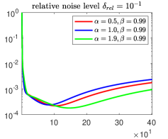
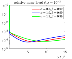
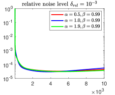
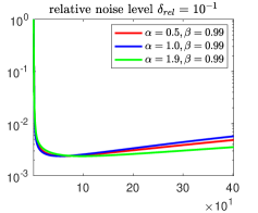
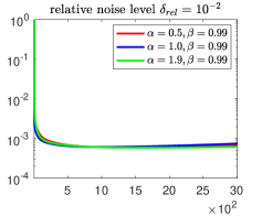
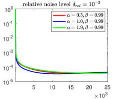
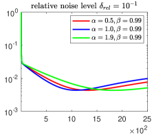
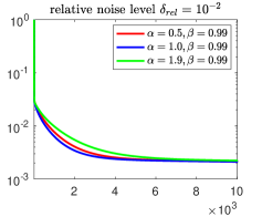
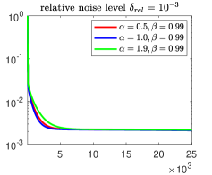
Figure 1. Reconstruction error of SVRG using various parameters of $\alpha,\beta$ and the relative noise level $\delta_{rel}$. The rows from top to bottom refer to phillips, gravity and shaw, respectively.

We first test the performance of Algorithm 2 by considering the system (6.1) with $N=5000$. For a given discrete model, the step-sizes depend on the update frequency $m$, $\alpha$ and $\beta$. We use $m=0.1N$. To illustrate the dependence of convergence on the magnitude of step-size, we consider the three groups of values: $(\alpha,\beta)=(0.5,0.99),(1.0,0.99)$ and $(1.9,0.99)$. Figure 1 depicts the corresponding relative mean square errors $\mathbb{E}\left[||x_{n}^{\delta}-x^{\dagger}||^{2}/||x^{\dagger}||^{2}\right]$ of reconstructions for the three model examples, where $n$ represent the number of epochs. These numerical plots demonstrate that the SVRG method exhibits the semi-convergence phenomenon, i.e., the iterate converges to the sought solution at the beginning and then starts to diverge after a critical number of iterations. Furthermore, the semi-convergence occurs earlier when the step-size is chosen by (2.3) with $(\alpha,\beta)=(1.0,0.99)$ which means this choice of $(\alpha,\beta)$ allows the iterates to rapidly produce a reconstruction result with minimal error, but also quickly diverge from the sought solution. The semi-convergence behavior poses a challenge in determining how to terminate the iteration to produce satisfactory reconstruction results. It is therefore necessary to consider a posteriori stopping rules.

Table 1. Numerical results for phillips model by SVRG, i.e. Algorithm 4 with $\gamma_{0}$ and $\gamma_{1}$ chosen by (2.3) using $\alpha=1$ and $\beta=0.99$, and Landwber method (1.3) with $\gamma=1/\|A\|^{2}$ terminated by the discrepancy principle with $\tau=1.01$.

$N$	$\delta_{rel}$	method	iteration	time (s)	relative error
1000	0.1	Landweber	19	0.0101	4.1590e-03
		SVRG: $m=N$	2.72	0.0156	2.4393e-03
		SVRG: $m=0.1N$	5.37	0.0080	3.4368e-03
	0.01	Landweber	102	0.0385	7.9908e-04
		SVRG: $m=N$	9.14	0.0525	1.1483e-03
		SVRG: $m=0.1N$	22.21	0.0277	1.0987e-03
	0.001	Landweber	3059	1.1237	9.6454e-05
		SVRG: $m=N$	245.77	1.2181	1.1943e-04
		SVRG: $m=0.1N$	638.62	0.6945	1.1686e-04
5000	0.1	Landweber	16	0.1570	5.9102e-03
		SVRG: $m=N$	2.03	0.4533	1.9841e-03
		SVRG: $m=0.1N$	3.11	0.1041	3.9575e-03
	0.01	Landweber	114	1.0965	6.5804e-04
		SVRG: $m=N$	5.28	1.1646	9.2306e-04
		SVRG: $m=0.1N$	13.41	0.4330	9.6879e-04
	0.001	Landweber	2690	25.294	1.5558e-04
		SVRG: $m=N$	93.57	20.208	1.6958e-04
		SVRG: $m=0.1N$	283.17	9.1490	1.6979e-04
10000	0.1	Landweber	16	0.6462	6.3237e-03
		SVRG: $m=N$	2.01	2.4825	1.7839e-03
		SVRG: $m=0.1N$	2.7	0.4334	3.6413e-03
	0.01	Landweber	116	3.9144	6.3945e-04
		SVRG: $m=N$	3.85	4.6586	7.9873e-04
		SVRG: $m=0.1N$	10.41	1.6302	8.7121e-04
	0.001	Landweber	3449	116.48	9.0028e-05
		SVRG: $m=N$	95.05	111.98	1.1096e-04
		SVRG: $m=0.1N$	268.72	44.136	1.0459e-04

Next we assume that the information on the noise level $\delta:=\|y^{\delta}-y\|$ is available and consider the SVRG method terminated by the discrepancy principle as described in Algorithm 4. We demonstrate the numerical performance of Algorithm 4 on the three model problems with $\gamma_{0}$ and $\gamma_{1}$ chosen by (2.3) with $\alpha=1.0,\beta=0.99$. In this study, we employ the Landweber method as our benchmark. For the comparison, the Landweber method (1.3) is initialized with $x_{0}=0$ with the constant step-size $\gamma=1/||A||^{2}$. The both methods are terminated by the discrepancy principle with $\tau=1.01$.

Table 2. Numerical results for gravity model by SVRG, i.e. Algorithm 4 with $\gamma_{0}$ and $\gamma_{1}$ chosen by (2.3) using $\alpha=1$ and $\beta=0.99$, and Landwber method (1.3) with $\gamma=1/\|A\|^{2}$ terminated by the discrepancy principle with $\tau=1.01$.

$N$	$\delta_{rel}$	method	iteration	time (s)	relative error
1000	0.1	Landweber	23	0.0091	6.8214e-03
		SVRG: $m=N$	2.52	0.0136	6.2835e-03
		SVRG: $m=0.1N$	4.54	0.0055	7.5344e-03
	0.01	Landweber	178	0.0618	2.0434e-03
		SVRG: $m=N$	12.72	0.0625	2.0389e-03
		SVRG: $m=0.1N$	34.03	0.0388	2.0621e-03
	0.001	Landweber	3774	1.0686	3.1782e-04
		SVRG: $m=N$	208.28	0.9407	3.1532e-04
		SVRG: $m=0.1N$	649.56	0.7182	3.2604e-04
5000	0.1	Landweber	22	0.2075	7.7204e-03
		SVRG: $m=N$	1.98	0.4385	5.6416e-03
		SVRG: $m=0.1N$	2.89	0.0938	7.4545e-03
	0.01	Landweber	249	2.2940	1.5475e-03
		SVRG: $m=N$	8.71	1.9899	1.5585e-03
		SVRG: $m=0.1N$	24.2	0.7469	1.6239e-03
	0.001	Landweber	4588	42.369	2.7350e-04
		SVRG: $m=N$	120.48	27.256	2.7895e-04
		SVRG: $m=0.1N$	377.31	12.120	2.7368e-04
10000	0.1	Landweber	22	0.7390	8.0617e-03
		SVRG: $m=N$	1.97	2.2943	4.6782e-03
		SVRG: $m=0.1N$	2.38	0.3695	6.5503e-03
	0.01	Landweber	275	9.0302	1.3574e-03
		SVRG: $m=N$	6.53	7.6368	1.4864e-03
		SVRG: $m=0.1N$	17.73	2.6020	1.4652e-03
	0.001	Landweber	4614	153.75	2.7504e-04
		SVRG: $m=N$	89.83	107.45	2.7817e-04
		SVRG: $m=0.1N$	288.95	43.520	2.7620e-04

The SVRG algorithm involves a hyperparameter, the update frequency $m$ of evaluating the full gradient, which is a key parameter for the performance and efficiency of the method. To assess the impact of the hyperparameter $m$ at different scales, we conduct a series of numerical experiments with $m=N$ and $m=0.1N$ for three different discretization levels $N=1000,5000,10000$. The numerical results for the three model problems are reported in Table 1, Table 2 and Table 3. In these tables, “iteration” represents the stopping index output by the discrepancy principle, and “time” and “relative error” report the corresponding execution time and the relative error at the output stopping index; for Algorithm 4 these quantities are calculated as the averages of 100 independent runs.

Table 3. Numerical results for shaw model by SVRG, i.e. Algorithm 4 with $\gamma_{0}$ and $\gamma_{1}$ chosen by (2.3) using $\alpha=1$ and $\beta=0.99$, and Landwber method (1.3) with $\gamma=1/\|A\|^{2}$ terminated by the discrepancy principle with $\tau=1.01$.

$N$	$\delta_{rel}$	method	iteration	time (s)	relative error
1000	0.1	Landweber	56	0.0183	3.3729e-02
		SVRG: $m=N$	4.82	0.0242	3.2753e-02
		SVRG: $m=0.1N$	11.94	0.0136	3.3493e-02
	0.01	Landweber	1732	0.5525	1.8242e-02
		SVRG: $m=N$	137.64	0.6567	1.8157e-02
		SVRG: $m=0.1N$	369.43	0.4109	1.8258e-02
	0.001	Landweber	27018	6.9767	2.5595e-03
		SVRG: $m=N$	2134.6	9.5064	2.5599e-03
		SVRG: $m=0.1N$	5761.6	6.3493	2.5602e-03
5000	0.1	Landweber	57	0.5280	3.5610e-02
		SVRG: $m=N$	2.75	0.6069	3.2465e-02
		SVRG: $m=0.1N$	6.53	0.2047	3.4849e-02
	0.01	Landweber	2743	25.450	1.4948e-02
		SVRG: $m=N$	102.45	22.853	1.4832e-02
		SVRG: $m=0.1N$	299.36	9.1962	1.4919e-02
	0.001	Landweber	29136	283.34	2.4354e-03
		SVRG: $m=N$	1077.3	240.26	2.4347e-03
		SVRG: $m=0.1N$	3152.11	100.75	2.4353e-03
10000	0.1	Landweber	58	1.9163	3.4329e-02
		SVRG: $m=N$	2.13	2.4791	3.0960e-02
		SVRG: $m=0.1N$	5.02	0.7598	3.3105e-02
	0.01	Landweber	3185	109.54	1.3195e-02
		SVRG: $m=N$	84.47	100.94	1.3165e-02
		SVRG: $m=0.1N$	252.86	41.515	1.3138e-02
	0.001	Landweber	29962	1048.3	2.4488e-03
		SVRG: $m=N$	792.24	924.37	2.4479e-03
		SVRG: $m=0.1N$	2366.75	371.18	2.4488e-03

The numerical results reveal several noteworthy observations. First, the results demonstrate that Algorithm 4 can be terminated after finite number of iterations and produces acceptable approximate solutions. Meanwhile, the relative error consistently decreases steadily as the noise level $\delta$ decreases, exhibiting the convergence behavior of the proposed method. In terms of accuracy (measured by the relative mean squared error), SVRG is competitive with the classical Landweber method for the three model problems. In most cases, the corresponding relative errors for the both methods are fairly close, and occasionally the relative error of the SVRG method can be even smaller than Landweber method. These observations are valid for all the examples, despite their dramatic difference in degree of ill-posedness and solution smoothness.

Note that each epoch in Algorithm 4 consists of a one-step of Landweber iteration which has complexity $O(NM)$ and an inner loop with $m$ iterations which has complexity $O(mM)$. Thus, the total complexity for each epoch of Algorithm 4 is $O((N+m)M)$. Consequently, if the algorithm is executed $n$ outer loops, the total computational complexity is $\mathcal{O}(n(N+m)M)$. Specifically, when $m=N$, one epoch in Algorithm 4 is equivalent to executing $2$ iterations of the Landweber method; and when $m=0.1N$, it is equivalent to executing $1.1$ times of Landweber steps. Therefore, from the perspective of computational complexity, the SVRG method is much more efficient than the Landweber method. For instance, in the gravity model with $\delta_{rel}=10^{-3},N=10000,m=0.1N$, the SVRG method executes $288.95\times 1.1\approx 318$ iterations of the Landweber method. This is only about $1/14.5$ of the 4614 iterations required by the Landweber method. However, since MATLAB optimizes matrix operations efficiently internally, directly using matrix operations is usually much more efficient than using loop iteration of matrix elements for calculation. Therefore, in the case of a small sample size ($N=1000$), although the theoretical computational complexity of the SVRG method is much lower than that of the Landweber method, the execution time of the algorithm is slightly higher. Even so, when handling large-scale problems ($N=5000,10000$), the SVRG method exhibits significant performance advantages over the traditional Landweber method, as traditional methods may require more iterations to achieve the same convergence standards in such scenarios.

Meanwhile, from the perspective of execution time results, we notice that the hyperparameter $m$ has a significant impact on the overall efficiency of the SVRG algorithm. In particular, a larger $m$ value means that more number of inner iterations need to be performed in each loop, which directly leads to a significant increase in the computational cost required for each epoch, especially when processing large-scale problems. In addition, too large $m$ makes little variance reduction at the final stage of each inner iteration part because the iterates could be far away the snapshot point, which is not favorable to the overall performance of the algorithm. By analyzing the experimental results of the three different models under the same relative noise levels $\delta_{rel}$ and discretization levels, we found that, compared to $m=N$, setting $m=0.1N$ significantly reduces execution time, achieving two to three times faster efficiency while maintaining accuracy comparable to the traditional Landweber method. This emphasizes the effectiveness of appropriately decreasing $m$ to reduce computational costs and obtain satisfactory reconstruction results without affecting the performance of the algorithm.

To further illustrate the performance of individual samples, we present the boxplots of the relative errors and epochs with the discretization level $N=10000$ for 100 simulations in Figure 2. On the box, the central mark is the median, and the bottom and top edges of the box indicate the 25th and 75 percentiles, respectively; the whiskers extend to the most extreme data points the algorithm considers to be not outliers, and the outliers are plotted individually using the “+” symbol. It is visible that the proposed method exhibits convergence. Meanwhile, we observe that the relative error $||x_{n_{\delta}}^{\delta}-x^{\dagger}||^{2}/\|x^{\dagger}\|^{2}$ increases with the relative noise level $\delta_{rel}$, and its distribution also broadens. However, the required number of epochs to fulfill the posteriori stopping indices decreases dramatically, as the relative noise level $\delta_{rel}$ increases, concurring with the preceding observation.

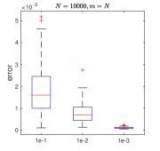
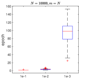
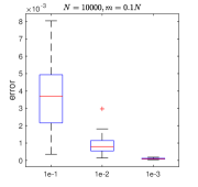
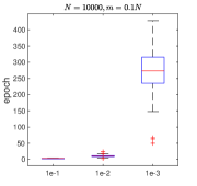
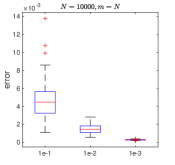
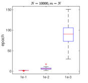
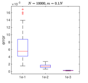
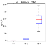
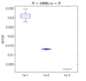
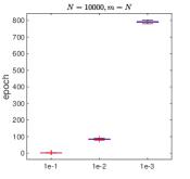
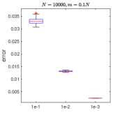
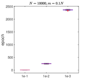
Figure 2. Boxplots of the relative error $||x_{n_{\delta}}^{\delta}-x^{\dagger}||^{2}/||x^{\dagger}||^{2}$ and the stopping index $n_{\delta}$ for the model probelms with $N=10000$. The rows from top to bottom refer to phillips, gravity and shaw respectively.

In order to visualize the performance, the reconstructed solutions of some individual runs are plotted in Figure 3. All these results demonstrate that the proposed method consistently produces satisfactory reconstruction results.

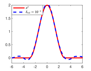
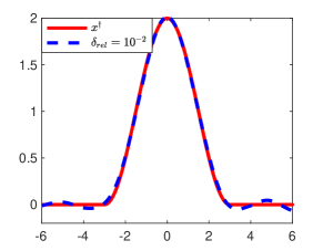
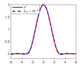
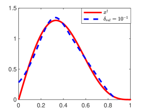
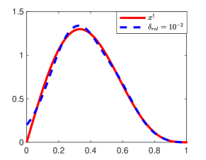
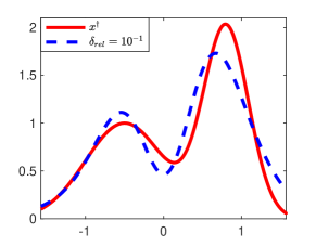
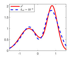
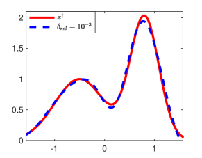
Figure 3. The sought solution $x^{\dagger}$ and the reconstruction results by SVRG using noisy data with various relative noise levels. The rows from top to bottom refer to phillips, gravity and shaw respectively.

7. Conclusion

Stochastic variance reduced gradient (SVRG) method is a prominent method for solving large scale well-posed optimization problems in machine learning and a variance reduction strategy has been introduced into the algorithm design to accelerate the stochastic gradient method. In this paper we applied the SVRG method to solve large scale linear ill-posed systems in Hilbert spaces. Under a benchmark source condition on the sought solution, we obtained a convergence rate result on the method when a stopping index is properly chosen. Based on this result and a perturbation argument we established a convergence result without using any source conditions. Furthermore, we considered the discrepancy principle to choose the stopping index and demonstrated that it terminates the SVRG method in finite many iteration steps almost surely. Various numerical results were reported which illustrate that the SVRG method can outperform the classical Landweber method for large scale ill-posed inverse problems. There are several questions that might deserve further investigation:

1. In the SVRG method we used constant step sizes $\gamma_{0}$ and $\gamma_{1}$. Is it possible to develop a convergence theory of the SVRG method using adaptive step sizes so that larger step size can be allowed to reduce the number of iterations and hence to speed up the method?

2. Our convergence theory for the SVRG method is for determining the $x_{0}$-minimal norm solutions. In applications, the sought solutions may have other a priori available features, such as nonnegativity, sparsity and so on. Is it possible to modify the SVRG method with a solid theoretical foundation so that it can capture such desired features?

3. Nonlinear ill-posed systems can arise from various tomography imaging problems. Can we extend the SVRG method to solve ill-posed systems in nonlinear setting?

References

- [1] Z. Allen-Zhu and Y. Yuan, Improved SVRG for non-strongly-convex or sum-of-non-convex Objectives, International Conference on Machine Learning, pp. 1080–1089, 2016.
- [2] M. Bertero, C. De Mol and E. R. Pike, Linear inverse problems with discrete data. I: General formulation and singular system analysis, Inverse Problems, l (1985), 301–330.
- [3] P. Brémaud, Probability theory and stochastic processes, Universitext, Springer, Cham, 2020.
- [4] A. Defazio, F. Bach and S. Lacoste-Julien, Saga: a fast incremental gradient method with support for non-strongly convex composite objectives, Proc. 27th Int. Conf. Adv. Neural Inf. Process. Syst., pp. 1646–1654, 2014.
- [5] H. W. Engl, M. Hanke and A. Neubauer, Regularization of Inverse Problems, Dordrecht, Kluwer, 1996.
- [6] P. C. Hansen, Regularization tools version 4.0 for Matlab 7.3, Numer. Algorithms, 46 (2007), 189–194.
- [7] R. Harikandeh, M. O. Ahmed, A. Virani, M. Schmidt, J. Konecny and S. Sallinen, Stop wasting my gradients: practical SVRG, Proc. 28th Int. Conf. Adv. Neural Inf. Process. Syst., pp. 2251–2259, 2015.
- [8] B. Jin and X. Lu, On the regularizing property of stochastic gradient descent, Inverse Problems, 35 (2019), no. 1, 015004, 27 pp.
- [9] B. Jin, Z. Zhou and J. Zou, An analysis of stochastic variance reduced gradient for linear inverse problems, Inverse Problems, 38 (2022), no. 2, 025009, 34 pp.
- [10] Q. Jin, On a regularized Levenberg-Marquardt method for solving nonlinear inverse problems, Numer. Math., 115 (2010), no. 2, 229–259.
- [11] Q. Jin, A general convergence analysis of some Newton-type methods for nonlinear inverse problems, SIAM J. Numer. Anal., 49 (2011), no. 2, 549–573.
- [12] Q. Jin, X. Lu and L. Zhang, Stochastic mirror descent method for linear ill-posed problems in Banach spaces, Inverse Problems, 39 (2023), no. 6, 065010, 39 pp.
- [13] R. Johnson and T. Zhang, Accelerating stochastic gradient descent using predictive variance reduction, Advances in Neural Information Processing Systems, 315–323, 2013.
- [14] F. Natterer,The Mathematics of Computerized Tomography, SIAM, Philadelphia, 2001.
- [15] L. M. Nguyen, J. Liu, K. Scheinberg and M. Takác, SARAH: a novel method for machine learning problems using stochastic recursive gradient, Proc. 34th Int. Conf. Machine Learning, PMLR, 70 (2017), 2613–2621.
- [16] N. Le Roux, M. Schmidt and F. Bach, A stochastic gradient method with an exponential convergence rate for strongly-convex optimization with finite training sets, Advances in Neural Information Processing System, 2663–2671, 2012.
- [17] S. Shalev-Shwartz and T. Zhang, Stochastic dual coordinate as- cent methods for regularized loss minimization, J. Mach. Learn. Res., 14 (2013), 567–599.
- [18] C. Tan, S. Ma, Y. H. Dai and Y. Qian, Barzilai–Borwein step size for stochastic gradient descent, Proc. 29th Int. Conf. Adv. Neural Inf. Process. Syst., 685–693, 2016.
- [19] L. Xiao and T. Zhang, A proximal stochastic gradient method with progressive variance reduction, SIAM Journal on Optimization, 24 (2014), no. 4, 2057––2075.
- [20] T. Yu, X. Liu, Y. H. Dai and J. Sun, Stochastic variance reduced gradient methods using a trust-region-like scheme, J. Sci. Comput., 87 (2021), no. 1, Paper No. 5, 24 pp.
- [21] L. Zhang, M. Mahdavi and R. Jin, Linear convergence with condition number independent access of full gradients, Advances in Neural Information Processing Systems, 980–988, 2013.
- [22] Y. Zhang and L. Xiao, Stochastic primal-dual coordinate method for regularized empirical risk minimization, Proc. Int. Conf. Mach. Learn., 2015, 353–361.