A modified interferometer to measure anyonic braiding statistics
Abstract
Existing quantum Hall interferometers measure twice the braiding phase, , of Abelian anyons, i.e. the phase accrued when one quasi-particle encircles another clockwise. We propose a modified Fabry–Pérot or Mach–Zehnder interferometer that can measure .
A major advance in the study of topological quantum phases of matter has been achieved through the first direct measurements of the expected fractional braiding statistics of the quasi-particles in the fractional quantum Hall effect using various quantum Hall interferometers [1, 2, 3, 4, 5, 6, 7, 8, 9, 10, 11, 12, 13, 14, 15, 16]. However, as was recently pointed out in Ref. [17], since these measurements effectively detect the phase accrued as one quasi-particle encircles an integer number of others, they measure twice the statistical phase, ; one particle encircling another is topologically equivalent to two exchanges of the same handedness. Among other things, this means that these interferometers could not distinguish bosons () from fermions ().
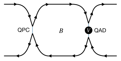
Here we propose a slightly more complex version of an interferometer that would directly measure .111The motivation here is similar to that in an earlier study [18, 19], in which the sign of the Josephson coupling between two conventional (s-wave) superconductors mediated by tunneling through a quantum dot can be switched from positive to negative depending on whether the dot is unoccupied or singly occupied; the negative Josephson coupling in the latter case derives from the Fermi statistics of the individual electrons that make up the Cooper pair. The geometry of the proposed interferometer is similar to one that was explored in a somewhat different context in Refs. [20] and [21]. The interferometer we have in mind is shown schematically in Fig. 1. The basic structure is of a conventional quantum Hall Fabry–Pérot interferometer, but with a quantum anti-dot (QAD) symmetrically located midway across one of the quantum point contact (QPC) junctions. (Our discussion applies essentially unchanged to a Mach–Zehnder interferometer [16] with the QAD midway across its junction). We assume that the tunneling from the upper (right-moving) edge state to the lower (left-moving) edge state at this junction occurs through a near-resonant two-step process through one of the bound states on the anti-dot.
Specifically, let signify the energy, relative to the chemical potential, of the relevant bound state. In the ground state of the system, this level is occupied by a quasi-particle if , while it is unoccupied if . By tuning a gate voltage, identified as in the figure, it is possible to tune through zero, i.e. through the resonance.222The quantization of the states on the anti-dot can be understood through semiclassical quantization of many-anyon bound states, as discussed in Ref. [22] and below. When , the dominant process simply involves a single quasi-particle tunneling from the upper edge, through the unoccupied near-resonant level, and on to the lower edge. When , on the other hand, the dominant process is a cooperative one in which the quasi-particle in the occupied near-resonant level first tunnels to the lower edge and then is replaced by a quasi-particle from the upper edge.333Note that these same two processes can equivalently be described in terms of cooperative versus simple resonant tunneling of a quasi-hole from the lower edge to the upper edge, respectively.
The interferometer is sensitive to the relative phase, (defined modulo ), between processes in which a quasi-particle tunnels through the first point contact and processes in which it tunnels through the second point contact. This phase can be expressed as
| (1) |
where is the effective magnetic flux quantum with the factional charge of the quasi-particle, is the area enclosed in the interferometer, is the applied perpendicular magnetic field, and are, respectively, the number of quasi-particles and quasi-holes enclosed in the interior of the interferometer, and is the statistical phase associated with the clockwise exchange of two quasi-particles.444Note that and are the phases associated with the clockwise transport of a quasi-particle around another quasi-particle and around a quasi-hole, respectively [23]. The new feature associated with the modified design of the interferometer is the last term, , where for the direct tunneling process through the anti-dot, and for the cooperative process. The origin of this term can be seen from considering the process in which a quasi-particle begins at the lower edge of the right point contact, propagates along the lower edge and tunnels to the upper edge at the left point contact, propagates back to the right point contact along the upper edge, and finally tunnels back to its original position. In the case of direct tunneling through the anti-dot, we have simply taken one quasi-particle around a closed path. But in the case of cooperative tunneling, in addition to this we have exchanged the quasi-particle that was originally on the anti-dot with the quasi-particle that was originally at the upper edge of the right point contact.
The idea, then, is to tune the anti-dot through resonance (from to ) and look for a phase shift in the interference pattern.555The shift of the phase should occur over a range of near corresponding to the larger of the width of the resonance and the temperature. In addition to the fact that this shift is a measure of rather than , an advantage of this design is that the shift is directly induced by a controlled variation of a gate voltage, rather than relying on an accidental (and unknown) rearrangement of quasi-particle occupations inside the interferometer. However, a possible confounding factor is that it may be difficult to distinguish a small shift in the enclosed area for the two different resonant processes from the desired statistical shift.666The interference pattern is typically explored by controlling both the magnetic field and the enclosed area by shifting the trajectory of the edge states with a gate.
Further considerations
We now discuss a few subtleties and details that underlie the above analysis:
1) As already mentioned, we need to assume that the Aharonov-Bohm phase accrued is independent of whether the tunneling process through the anti-dot is the direct process or the cooperative one. It is plausible that this condition is approximately satisfied under various reasonable circumstances, but we have not determined an unambiguous way to insure this. Empirically, in determining whether this condition is satisfied, a first pass should be to look for the expected -phase shifts in the integer quantum Hall regime.
2) As an aid to intuition, we consider a simple model problem in which a similar process can be used to distinguish bosons from fermions. Consider a system described by the Hamiltonian
| (2) |
where and are either bosonic or fermionic operators that create, respectively, a particle with zero energy on the upper or lower edge, and creates a particle on the QAD. Here is the energy of the state on the QAD, is the number of particles on the QAD, and (relevant only for the case of bosons) is the repulsion between two particles on the QAD. To zeroth order in the tunneling (i.e. when ), the ground state of the QAD has for and for . (We will not treat where, in the bosonic case, .)
The effective Hamiltonian that describes the coupling between the edge-states to second order in is
| (3) |
where, in the fermionic case,
| (4) | ||||
while in the bosonic case, is as in Eq. (4), and
| (5) | ||||
In both cases, the magnitude of grows as one approaches the resonance condition, ; however, in the bosonic case, the phase of remains the same independent of the sign of , while in the fermionic case there is an abrupt phase shift.777Needless to say, the singular behavior as is rounded by higher order terms when . Indeed, in the fermionic version, this is actually a non-interacting problem and readily solved exactly; in this case, the change in the sign of upon tuning through can be understood as the difference between tunneling through an intermediate state with energy greater or less than that of the edge state. However, viewed from a many-body perspective, where the Fermi statistics act as an effective interaction, the change in the sign of as crosses zero is directly related to the fact that for , the tunneling process is direct, while for it is an exchange process. That this is not simply a question of perspective is established by the comparison with the bosonic case. The overall phase of is of course a matter of convention; it can be altered by a simple redefinition , . But the abrupt change in the phase of as changes sign is independent of this ambiguity.
3) The spectrum of bound states associated with the anti-dot is ultimately a many-body problem, as interaction effects are always essential to the existence of a fractional quantum Hall state. All that is needed for our treatment, however, is a quasi-particle description of the lowest-lying excited states of the anti-dot—either with one added quasi-particle (when ) or one added quasi-hole (when ). The essence of this problem can be understood on the basis of a semiclassical treatment along similar lines as the analysis in Ref. [22]. We model the QAD as a potential maximum that is smooth on the scale of the magnetic length and weak enough to not mix Landau levels. The quasi-hole bound states of the anti-dot, with energies , are associated with semiclassical orbits along equal-potential contours of . The quantization conditions are
| (6) |
where is the area enclosed by the contour with , each is a nonnegative integer, and is the number of quasi-holes enclosed by the trajectory of quasi-hole . The ground state with quasi-holes, , is obtained by occupying the first orbitals which satisfy Eq. (6), , with all .
We take the near-resonant level to be the th orbital, and . Thus, when , the ground state of the QAD is and the first excited many-body state is (the lowest-energy state with one less quasi-hole, i.e. one added quasi-particle). When , the ground state is instead and the first excited state is .888In going from the ground state to the ground state , we assume that the quasi-hole removed from the QAD is trapped in some distant region of the sample, outside the interferometer.
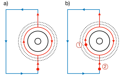
Now consider the near-resonant direct tunneling of a quasi-hole through the QAD when . Semiclassically, this corresponds to a coherent sum over trajectories in which the quasi-hole arrives with energy , orbits times around the contour , and departs, as depicted in Fig. 2a. We can assign a definite phase to each trajectory if we append a circuit of the quasi-hole around the body of the interferometer to return it to its starting position. The total phase factor for a trajectory includes both the Aharonov-Bohm phase corresponding to the enclosed magnetic flux and the statistical phase associated with anyon braiding ( for each clockwise exchange of quasi-holes, or each time a quasi-hole encircles another clockwise). The resonance condition, that the trajectories with different interfere constructively, is the same as the quantization condition (6), which ensures that the total phase accrued during each full orbit around the QAD is a multiple of . Similarly, the near-resonant cooperative tunneling process of a quasi-hole when corresponds to a coherent sum over trajectories in which a quasi-hole originally on the QAD with energy orbits times around the contour and departs, after which another quasi-hole with energy arrives and orbits times around the same contour, as depicted in Fig. 2b.
To compute the relative phase between the direct tunneling process and the cooperative one, we note that in either case, as discussed above, the total phase accrued during a full orbit around the anti-dot is a multiple of . Therefore it suffices to compare the direct trajectory with to the cooperative trajectory with . These differ in that the latter involves a counter-clockwise exchange of quasi-holes, whereas the former does not, and hence the relative phase is .999Strictly speaking, we should compare trajectories in which the quasi-holes start and end at the same locations to unambiguously determine the relative phase. This is not quite the case in the discussion above because, in the direct trajectory , the second quasi-hole is located in a distant region of the sample (not shown in the figure). However, it suffices to consider a modified trajectory in which this quasi-hole starts on the QAD, adiabatically moves to the distant location along some path , and then, after the direct tunneling process has concluded, returns to the QAD along the inverse path . By construction, the trajectories and carry the same phase, and the latter can be directly compared to the cooperative trajectory. Recalling that the direct quasi-hole tunneling process corresponds to the cooperative quasi-particle process, and vice versa, we recover the term in Eq. (1).
4) We have also analyzed the problem in terms of the Berry phase accrued for various assumed patterns of adiabatic motion of two quasi-holes using the wave-function approach of Arovas, Schrieffer and Wilczek [23]. The result has a simple interpretation in terms of flux attachment in that the accrued phase along any closed path is proportional to the expectation value of the enclosed charge. However, not surprisingly, the result depends in detail on the precise location of the assumed trajectory followed, and so does not obviously help to resolve the important issue of disentangling the statistical from the geometric contributions to the phase.
5) While the statistical interaction between quasi-particles is the longest-range interaction, other shorter-range interactions manifestly exist as well. These can result in geometric differences in the paths followed by quasi-particles undergoing direct versus cooperative tunneling processes, which in turn can result in differences in the Berry phase that have nothing to do with braiding statistics. For this reason, we do not necessarily expect the present measurement to be as precise as the measurement of associated with braiding about a quasi-particle in the bulk, as the latter can in principle be spatially far separated from the propagating modes of the interferometer. However, given an accurate measurement of , the present interferometer need only be accurate enough to distinguish from .
6) The above analysis applies directly to simple “Laughlin” states with Abelian anyons and (under appropriate conditions, i.e. in the absence of any non-trivial form of edge reconstruction) a single edge mode. The extension of these considerations to hierarchical states [24] and most importantly to states with non-Abelian anyons [25, 26, 27] is presumably possible.
Acknowledgements.
We acknowledge helpful comments from Moty Heiblum, Patrick Lee, Hans Hansson, Steven Simon, Claudio Chamon, Eduardo Fradkin, and Nicholas Read. This work was supported in part by the Department of Energy, Office of Basic Energy Sciences, under contract no. DE AC02-76SF00515 (SAK and CM), and in part by the Gordon and Betty Moore Foundation’s EPiQS Initiative through GBMF8686 (CM).References
- Nakamura et al. [2020] J. Nakamura, S. Liang, G. C. Gardner, and M. J. Manfra, Direct observation of anyonic braiding statistics, Nature Physics 16, 931 (2020).
- Nakamura et al. [2023] J. Nakamura, S. Liang, G. C. Gardner, and M. J. Manfra, Fabry-Pérot interferometry at the fractional quantum Hall state, Physical Review X 13, 041012 (2023).
- Kundu et al. [2023] H. K. Kundu, S. Biswas, N. Ofek, V. Umansky, and M. Heiblum, Anyonic interference and braiding phase in a Mach–Zehnder interferometer, Nature Physics 19, 515 (2023).
- Willett et al. [2023] R. L. Willett, K. Shtengel, C. Nayak, L. N. Pfeiffer, Y. J. Chung, M. L. Peabody, K. W. Baldwin, and K. W. West, Interference measurements of non-Abelian & Abelian quasiparticle braiding, Physical Review X 13, 011028 (2023).
- McClure et al. [2012] D. T. McClure, W. Chang, C. M. Marcus, L. N. Pfeiffer, and K. W. West, Fabry–Perot interferometry with fractional charges, Physical Review Letters 108, 256804 (2012).
- [6] A. Young, private communication.
- Kivelson and Marcus [a] S. A. Kivelson and C. M. Marcus, At last! Measurement of fractional statistics, JCCM, July 2020, 02. Recommendation on Ref. [1].
- Kivelson and Marcus [b] S. A. Kivelson and C. M. Marcus, Progress measuring fractional quantum numbers in quantum Hall interferometers, JCCM, June 2023, 01. Recommendation on Ref. [2].
- Feldman and Halperin [2022] D. E. Feldman and B. I. Halperin, Robustness of quantum Hall interferometry, Physical Review B 105, 165310 (2022).
- Chamon et al. [1997] C. d. C. Chamon, D. E. Freed, S. A. Kivelson, S. L. Sondhi, and X. G. Wen, Two point-contact interferometer for quantum Hall systems, Physical Review B 55, 2331 (1997).
- Camino et al. [2005] F. E. Camino, W. Zhou, and V. J. Goldman, Aharonov-Bohm superperiod in a Laughlin quasiparticle interferometer, Physical Review Letters 95, 246802 (2005).
- Camino et al. [2007] F. E. Camino, W. Zhou, and V. J. Goldman, Laughlin quasiparticle primary-filling interferometer, Physical Review Letters 98, 076805 (2007).
- Willett et al. [2009] R. L. Willett, L. N. Pfeiffer, and K. W. West, Measurement of filling factor 5/2 quasiparticle interference with observation of charge e/4 and e/2 period oscillations, Proceedings of the National Academy of Sciences 106, 8853 (2009).
- Ofek et al. [2010] N. Ofek, A. Bid, M. Heiblum, A. Stern, V. Umansky, and D. Mahalu, Role of interactions in an electronic Fabry–Perot interferometer operating in the quantum Hall effect regime, Proceedings of the National Academy of Sciences 107, 5276 (2010).
- Halperin et al. [2011] B. I. Halperin, A. Stern, I. Neder, and B. Rosenow, Theory of the Fabry–Pérot quantum Hall interferometer, Physical Review B 83, 155440 (2011).
- Ji et al. [2003] Y. Ji, Y. Chung, D. Sprinzak, M. Heiblum, D. Mahalu, and H. Shtrikman, An electronic Mach–Zehnder interferometer, Nature 422, 415 (2003).
- Read and Das Sarma [2024] N. Read and S. Das Sarma, Clarification of braiding statistics in Fabry–Perot interferometry, Nature Physics 20, 381 (2024).
- Spivak and Kivelson [1991] B. I. Spivak and S. A. Kivelson, Negative local superfluid densities: The difference between dirty superconductors and dirty Bose liquids, Physical Review B 43, 3740 (1991).
- Razmadze et al. [2020] D. Razmadze, E. C. T. O’Farrell, P. Krogstrup, and C. M. Marcus, Quantum dot parity effects in trivial and topological Josephson junctions, Physical Review Letters 125, 116803 (2020).
- Yacoby et al. [1995] A. Yacoby, M. Heiblum, D. Mahalu, and H. Shtrikman, Coherence and phase sensitive measurements in a quantum dot, Physical Review Letters 74, 4047 (1995).
- Schuster et al. [1997] R. Schuster, E. Buks, M. Heiblum, D. Mahalu, V. Umansky, and H. Shtrikman, Phase measurement in a quantum dot via a double-slit interference experiment, Nature 385, 417 (1997).
- Kivelson [1990] S. A. Kivelson, Semiclassical theory of localized many-anyon states, Physical Review Letters 65, 3369 (1990).
- Arovas et al. [1984] D. Arovas, J. R. Schrieffer, and F. Wilczek, Fractional statistics and the quantum Hall effect, Physical Review Letters 53, 722 (1984).
- Jain et al. [1993] J. K. Jain, S. A. Kivelson, and D. J. Thouless, Proposed measurement of an effective flux quantum in the fractional quantum Hall effect, Physical Review Letters 71, 3003 (1993).
- Stern and Halperin [2006] A. Stern and B. I. Halperin, Proposed experiments to probe the non-Abelian quantum Hall state, Physical Review Letters 96, 016802 (2006).
- Bonderson et al. [2006] P. Bonderson, A. Kitaev, and K. Shtengel, Detecting non-Abelian statistics in the fractional quantum Hall state, Physical Review Letters 96, 016803 (2006).
- Feldman and Kitaev [2006] D. E. Feldman and A. Kitaev, Detecting non-Abelian statistics with an electronic Mach–Zehnder interferometer, Physical Review Letters 97, 186803 (2006).