The Impact of Feedback-driven Outflows on Bar Formation

Abstract

We investigate the coupling between the temporal variation from galaxy-formation feedback and the bar instability. We show that fluctuations from mass outflow on star-formation time scales affect the radial motion of disk orbits. The resulting incoherence in orbital phase leads to the disruption of the bar-forming dynamics. Bar formation is suppressed in starburst galaxies that have fluctuation time scales within the range $10<\tau<200{\rm\,Myr}$ with repeated events with wind mass $\sim 15\%$ of the disk within $\sim 0.5$ scale lengths or 1.4% of the total disk mass. The work done by feedback is capable of reducing the amplitude or, with enough amplitude, destroying an existing bar. AGN feedback with similar amplitude and timescales would have similar behavior.

To model the dynamics of the coupling and interpret the results of the full N-body simulations, we introduce a generalization of the Hamiltonian mean-field (HMF) model, drawing inspiration from the Lynden-Bell (1979) mechanism for bar growth. Our non-linear BarHMF model is designed to reproduce linear perturbation theory in the low-amplitude limit. Notably, without star-formation feedback, this model exhibits exponential growth whose rate depends on disk mass and reproduces the expected saturation of bar growth observed in N-body simulations. We describe several promising applications of the BarHMF model beyond this study.

1 Introduction

Bar are a ubiquitous feature of disk galaxies: at least 50% of all disk galaxies in the local universe are barred (e.g. Aguerri et al., 2009). Bars were among the first instabilities to be found and studied in N-body simulations (Hohl, 1971; Ostriker and Peebles, 1973). They are predicted to be important drivers of secular evolution (Lynden-Bell and Kalnajs, 1972; Tremaine and Weinberg, 1984) and barred galaxies may require secular evolution to create their present-day morphology (Athanassoula, 2003). In this way, their coupling to the baryonic, and the dark-matter components of a galaxy through cosmic time make their dynamical details an important diagnostic of galaxy formation and evolution. The bulk of the stellar population takes part in the bar instability, making bars morphologically distinct and straightforwardly observed in the near-infrared. Indeed, recent analyses of JWST NIRCam images suggest that some bar systems may have been active for many gigayears (Guo et al., 2023). An understanding of the formation time and duty cycle of bar-driven evolution requires a thorough understanding of the dynamical mechanisms that affect bar evolution.

Both by technical necessity and experimental design, most theoretical and numerical studies of barred galaxy dynamics begin with quiescent equilibria chosen to be unstable to bar formation. While our dynamical insight follows from such carefully controlled dynamical experiments (e.g. Petersen et al., 2019, 2021), we are well-aware that galaxies continue to accrete mass through cosmic time, but we have not given this time dependence detailed attention dynamically. Nonetheless, the key dynamical principles for bar formation and subsequent secular evolution are well-understood after decades of study (see Binney and Tremaine, 2008). On the other hand, a wide variety of time-dependent feedback processes are necessary to produce the galaxies in cosmological simulations (e.g. Ceverino and Klypin, 2009; Kormendy and Ho, 2013). For example, the work done on the gravitational potential by this feedback has a natural time scale and amplitude. The time scale is approximately 10–200 Myr based on theory and estimated from observations (Heckman et al., 1990; Hopkins and Hernquist, 2010). The amount of mass lost from the disk, and hence work done on the disk gravitational potential is much harder to estimate. Star formation efficiencies in a star forming event are estimated to be ${\cal O}(0.1)$ (Combes et al., 2013).

The bar instability itself results from the precession of apocenter positions of nearby orbits toward its self-induced quadrupole distortion. If a non-trivial fraction of the remaining gas is heated or launched into halo during a star-formation event, the work done on the gravitational potential changes the orbital actions of stars in the disk. These event time scales are similar to the characteristic orbital times in the disk. Thus, the resulting star-formation-driven fluctuations can affect the orbital coherence required for bar formation. We expect this coupling to be particularly important during the peak of star formation. During this epoch at redshifts of $z=2$–$3$ often called cosmic noon, galaxies formed about half of their current stellar mass (Madau and Dickinson, 2014), and the effect of feedback will be maximal and most likely significant source of gravitational fluctuations. While widely explored in suites of galaxy-formation simulations, these processes have not been given the detailed dynamical attention they deserve. The description of this coupling between the feedback fluctuations and the bar instability mechanism and estimating the importance of feedback to bar formation is the main goal of this paper.

There are two main feedback mechanisms in cosmological simulations that have regulatory affect on the baryonic history: active galactic nuclei (AGN) and star formation (SF). Presumably, both play a role in the self regulation necessary to achieve the observed characteristics of present day galaxies. Both AGN winds and the interaction of supernova feedback with their surrounding gas through the injection of energy and momentum can lead to a feedback loop regulating ongoing SF. An effective feedback loop requires heating or removing a large fraction of the disk’s cold gas by winds and fountains. A variety of sub-resolution prescriptions have been employed to achieve this. Regardless of the details of the microphysics, these outflow events are episodic, not continuous. Because these events tend to be centrally dominated with characterstic dynamical times of $10<\tau<200\,\mbox{Myr}$, outflow events will provide gravitational fluctuations to the axisymmetric field of the disk. Similar to the regulation of the SF process, an effect on orbital dynamics does not demand that the outflow to escape from the galaxy; most of the required gravitational work over the first kiloparsec.

AGN processes are known to vary on short time scales and inferred to vary on longer scales as well (Sartori et al., 2018). Presumably, these long scales are governed by dynamical time scales typical of accretion and merger events which are similar to SF feedback time scales. AGN feedback is centrally dominated by definition. While we will interpret our results using the time scales and amplitudes typical of SF feedback in this work, the constraints from dynamical coupling proposed here could be applied to long-term epochs of AGN activity as well.

Feedback processes and galactic winds specifically have been well-reviewed over many years (e.g. Veilleux et al., 2005; King and Pounds, 2015; Zhang, 2018). The importance of the physical details in modeling SF regulation is also well appreciated. For example, Governato et al. (2007) remarked that subgrid star formation feedback tended to make the disk more stable against bar formation by reducing the stellar disk. Since then, simulations with higher resolution and sophisticated subgrid prescriptions have demonstrated large variance and intricate coupling between outflow, re-accretion of gas, and subsequent star formation with bar formation, even in the same simulation suite Zana et al. (e.g. 2019).

We will side-step the physical complexity of heating and momentum transfer in this paper. Rather, we adopt a simple Markov jump process that parameterizes the feedback by the time between SF events and the work done during SF events. We assume that most of the gas resettles on the disk at approximately the same timescale as the time between events. We investigate the dependence on the fluctuation amplitude and time scales that are required to disrupt bar formation. For our simulations, we choose an exponential disk and live dark-matter halo with masses typical of typical of a Milky-Way-like galaxy at cosmic noon.

The model adopted for this study is not intended to be realistic in the cosmological structure formation sense; neither our disk or halo accretes new material in time. For this reason, we focus on evolution times $<4\,\mbox{Gyr}$. Similarly, our simulations do not include satellite and sub-structure interactions. Rather, this suite is intended explore the dynamics of the coupling mechanism and to address two particular questions: (1) What is the stochastic frequency required to disrupt bar formation? (2) What is the amplitude of the work done required to disrupt bar formation? While inspired by feedback, the proposed dynamical mechanism is generic and intended to provide a framework for interpreting more realistic simulations.

Our primary model is chosen to form a bar in the absence of potential fluctuations with a disk mass of approximately $M_{disk}=5\times 10^{9}{\rm\,M_{\odot}}$ with $M_{halo}=10^{12}{\rm\,M_{\odot}}$. The system is not strongly bar unstable owing to its relatively low, sub-maximal disk mass. We show that bar formation is suppressed for starbursts with characteristic periods in range $10<\tau<200\,\mbox{Myr}$. Sufficient blow out amplitude is approximately $15\%$ of the baryonic mass inside of $0.5$ disk scale lengths.

Much has been written about the tension between the general observation of bar rotating near corotation (so-called fast bars, e.g. Fragkoudi et al. 2021) while secular theory predicts a rapid slowing of the bar pattern speed caused by global torques with the disk and halo. There are many possible caveats to this naive picture. However, this simple fluctuation-driven mechanism may stave off bar formation until well after cosmic noon. This could help explain the apparent dynamical youth of observed bars in the present-day universe.

The plan for this paper is as follows. Section 2 describes our galaxy mass profiles (Sec. 2.1), summarizes our N-body simulations of the disk and halo (Sec. 2.2), defines the parametrization of the feedback mechanism (Sec. 2.4), and the describes the new hybrid perturbation-theory based simulation (Sec. 2.5) used to provide dynamical insight for the feedback coupling to bar dynamics. Specifically, we adopt the tools of Hamiltonian perturbation theory to isolate the single degree of freedom that causes the outer apsides of disk orbits to collect along a diameter. This is the bar-formation mechanism described in Lynden-Bell (1979). It is derived by performing a change of angular coordinates where one of the angles describes the motion with respect to the inner-Lindblad resonance. Near resonance, the angular speed of this angle is much slower than the rapid variation of the star about its orbit radially. This allows us to average of the radial motion and reduce the dimensionality. Appendix B develops this idea into a particle simulation method. The main results are described in Section 3, beginning with a demonstration of the main result in Section 3.1 followed description of the primary model without star formation feedback in Section 3.2. Sections 3.3.1 and 3.3.2 describe the amplitudes and frequencies of the feedback process necessary to suppress the bar instability. Section 3.3.4 presents a dynamical mechanism for the noise coupling in the reduced model and compares it to the results from the full N-body simulations. We conclude with a summary and discussion in Section 4.

2 Methods

2.1 Galaxy model

We use virial units for length and mass, $R_{vir}$ and $M_{vir}$ respectively, with gravitational constant $G=1$ for all simulations described here and refer to those as system units. We present our results scaled to the Milky Way throughout to give physical context. We adopt $R_{vir}=300{\rm\,kpc}$ and $M_{vir}=1.4\times 10^{12}{\rm\,M_{\odot}}$ and use gigayears (Gyr) for time units. The system time units are $T_{vir}\equiv(R_{vir}^{3}/GM_{vir})^{1/2}\approx 2$ Gyr; or 1 Gyr is approximately 0.5 system time units.

2.1.1 Dark-matter halo

For our primary model, we adopt a modified NFW (Navarro et al., 1997) dark matter halo with concentration $c$, whose density is given by

$$\rho_{\rm halo}(r)\propto\left(r+r_{c}\right)^{-1}\left(r+r_{s}\right)^{-2}$$ (1)

where $r_{s}\equiv R_{\rm vir}/c$ is the scale radius, and $r_{c}\ll r_{s}$ is a radius that sets the size of the core. In this paper, core radius is is numerical convenience only and set to a value smaller than any astronomically relevant scale, typically several parsecs. We adopt $c=15$ for our dark matter halo which provides an acceptable representation of the rotation curve when scaled to the Milky Way. This is slightly more concentrated that the mean from Diemer and Kravtsov (2015) but within the variance measured from simulations.

In practice, we choose a more general profile family that includes the NFW model to explore the dynamical effect of changing the background profile from shallow to steep and enforce a finite total mass. Specifically, we modify a two-power halo model with an error function truncation of the following form:

$$\rho_{\alpha\beta}(r)=\frac{\rho_{0}r_{s}^{\alpha+\beta}}{(r+r_{c})^{\alpha}(r+r_{s})^{\beta}}\left\{\frac{1+\mathrm{erf}\left[(r_{t}-r)/r_{w}\right]}{2}\right\}.$$ (2)

where $\rho_{0}$ is a normalization set by the chosen mass. This is equivalent to equation (1) for $\alpha=1$ and $\beta=2$, and $r_{t}=\infty$. The outer truncation radius $r_{t}$ and truncation width $r_{w}$ are chosen to be 300 kpc and 60 kpc, respectively. For our primary model, we set $\alpha=1$, $\beta=2$, $r_{c}=4.5{\rm\,pc}$. We explore the effect of different $\alpha$ in Appendix B.4.

While one may debate the merits of a purely collisionless dark matter particle, axion dark matter, ‘fuzzy’ dark matter (Hu et al., 2000; Hui et al., 2017), or other descriptions of dark matter, the necessity of exploring the interaction between baryonic and unseen components via gravity may not be ignored. Dark matter will respond gravitationally to baryonic matter and different dark-matter responses can produce observable signatures. Rigidity in halos has been noted to limit bar growth (Polyachenko et al., 2016; Sellwood, 2016) as is clear from dynamics of secular evolution (Athanassoula, 2003), and so we emphasize that the live halo inclusion is crucial to recover the dynamics of the standard $\Lambda$CDM scenario. Specifically, both the fraction of gravitational support from the halo and the resonant coupling will affect bar growth, although we will not explore that sensitivity in this paper. There are many other parameters that may be adjusted in the creation of a halo which we do not explore here: triaxiality and spin are two that are addressed by others (Athanassoula et al., 2013; Aumer et al., 2016; Collier et al., 2018a, b). However, we do not expect either of these to qualitatively change the dynamical features explored in this work.

2.1.2 Disk

The simulations begin with an exponential disk of surface density

$$\Sigma_{\rm disk}(r)=\frac{M_{\rm d}}{2\pi a^{2}}\exp\left(-\frac{r}{a}\right)$$ (3)

where $M_{d}$ is the disk mass, and $a\equiv 0.01R_{\rm vir}=3{\rm\,kpc}$ is the disk scale length. We assume that the disk remains thin with no vertical response to further restrict the dynamical degrees of freedom for this simple proof-of-concept investigation.

We select the initial positions in the disk via acceptance–rejection algorithm using equation (3). We select the velocities by solving the Jeans equations (Binney and Tremaine, 2008) with an axisymmetric velocity ellipsoid in the disk plane ($\sigma_{r}\equiv\sigma_{\phi}$). We characterize the radial velocity dispersion using the Toomre $Q$ parameter,

$$\sigma_{r}^{2}(r)=\frac{3.36\Sigma(r)Q}{\Omega_{r}(r)}$$ (4)

where $\Sigma(r)$ is the disk surface density, and the radial frequency, $\Omega_{r}$, is given by

$$\Omega_{r}^{2}(r)=r\frac{d\Omega_{\phi}^{2}}{dr}+4\Omega_{\phi}^{2}.$$ (5)

where $\Omega_{\phi}$ is the azimuthal frequency. See Section 2.3 for additional details. The circular velocity curve for this model is shown in Figure 4. The rise in the inner few kiloparsecs promotes bar growth by design.

2.2 N-body method

We require a description of the gravitational potential and force vector at all points in physical space to compute the time evolution for an N-body system. We accomplish this using a orthogonal basis set of density-potential pairs that simultaneously solve the Poisson equation. This is the so-called a biorthgonal basis. We generate density-potential pairs using the basis function expansion (BFE) algorithm described in Weinberg (1999) and implemented in exp, our soon-to-be released BFE N-body and analysis code. In the BFE method (Clutton-Brock, 1972, 1973; Hernquist and Ostriker, 1992), a system of biorthogonal potential-density pairs are calculated and used to approximate the potential and force fields in the system. In our approach, the functions are calculated by numerically solving the Sturm-Liouville equation for eigenfunctions of the Laplacian. The full method is described precisely in Petersen et al. (2022).

exp optimally represents the BFE for halos with radial basis functions determined by the target density profile and spherical harmonics. The lowest-order $l=0,m=0$ basis function matches the potential and density of the equilibrium. The overall fields of the halo are described by $\left(l_{\rm halo}+1\right)^{2}\times n_{\rm halo}$ terms, where $l_{\rm halo}$ is the maximum order of spherical harmonics and $n_{\rm halo}$ is the maximum order of radial terms per $l$ order. For simulations and analyses in this paper, we use a maximum harmonic order $l_{\mbox{\tiny max}}=6$ and maximum radial order $n_{\mbox{\tiny max}}=20$ using the Sturm-Liouville basis conditioned on each particular input model. While the quality of the expansion is center dependent, the basis can follow any displacement from the center for sufficiently large particle number and large values of $l_{\mbox{\tiny max}}$ and $n_{\mbox{\tiny max}}$. The choices of $l_{\mbox{\tiny max}}=6$ and $n_{\mbox{\tiny max}}=20$ allow us follow center displacements seen in our simulations. The resulting series of coefficients fully describe time dependence of the gravitational field produced by the N-body evolution.

Appropriate basis functions for a three-dimensional cylindrical disk are described in Petersen et al. (2022). Here, we use a recently-implemented special-purpose two-dimensional cylindrical disk basis that is described in Appendix A. This focuses our dynamical attention on the two degrees of freedom essential to create a bar: the radial and azimuthal motion. We have demonstrated that same results are obtained for the full three-dimensional simulations in selected cases. Future work will include coupling to the vertical motion from possibly asymmetric outflows.

In summary, exp allows for a straightforward calculation of the gravitational potential from the mass distribution through time. The key limitation of the BFE method lies in the loss of flexibility owing to the truncation of the expansion series: large deviations from the equilibrium disk or halo will not be well represented. Although the basis is formally complete, our truncated version limits the variations that can be accurately reconstructed. Despite this, basis functions can be a powerful tool to gain physical insight; analogous to traditional Fourier analysis, a BFE identifies spatial scales and locations responsible for the model evolution. In particular, this paper investigates relatively low-amplitude, large-scale distortions which are well represented by the expansion.

2.3 Initial conditions

We generate realizations with $10^{6}$ disk particles and $10^{7}$ halo particles from the models in Sections 2.1.1 and 2.1.2 using the following algorithm:

1. The halo gravitational potential is modified to contain the monopole component of the exponential disk. The halo phase space distribution is then realized using Eddington inversion (e.g. Binney and Tremaine, 2008).

2. The disk phase space is generated using Jeans’ equations as described in Section 2.1.2.

3. The halo phase-space distribution is relaxed in the presence of the potential generated by the disk particle distribution using the exp potential solver for 4 Gyr ($2T_{vir}$). The force felt by the halo from the halo’s own self gravity is restricted to $m=0$ terms during this relaxation phase. The force felt by the halo from the disk is the disk’s gravity at $T=0$ for the axisymmetric component $m=0$ only.

4. The disk phase space is regenerated using Jeans’ equations as described in Section 2.1.2 using the gravitational potential of the halo distribution at the end of the relaxation step.

5. The disk phase-space distribution is then relaxed in the presence of the potential generated by the halo particle distribution using the exp potential solver for 4 Gyr. The force felt by the disk from the disk’s own self gravity is restricted to the $m=0$ term. The force felt by the disk from the halo is the halo’s gravity for the $m=0$ axisymmetric component only frozen at the beginning of this simulation.

6. The phase space distributions for the halo at the end of Step 3 and the disk at the end of Step 5 are the phase-space initial conditions for the simulations reported here.

This algorithm is enabled by the basis-function approach that underlies exp. In particular, the BFE approach used in exp provides a separate basis for each component (disk and halo, here) and each the expansion terms for basis may be applied selectively or frozen in time. For example, in Step 3 we allow only the axisymmetric force of the halo to obtain the new spheroidal equilibrium in the presence of the disk while preventing the natural halo modes from influencing the initial conditions. The resulting initial conditions are very close to feature-free to start. The initial condition realization described here has also been discussed in Petersen et al. (2022).

2.4 Perturbation scheme

We assume that a starburst can be modeled as a stochastic process in the inner galaxy disk that causes a sudden loss of fraction $\epsilon$ of the enclosed mass within radius $R_{burst}\equiv\lambda a$ where $a$ is the disk scale length. The lost mass is assumed to be fall back onto the disk over some characteristic period $P_{acc}$. This emulates a galactic fountain and the subsequent resettling of cooling gas. The perturbation is modeled mathematically as a Markov jump process with two characteristic frequencies: one that describes the star-burst frequency, $1/\tau_{1}$, and one that describes the re-accretion time, $\tau_{2}=P_{acc}$. Let $\tau_{dyn}$ decribe the dynamic time scale. Physical consistency implies that $\tau_{dyn}\mathrel{\hbox{\hbox to0.0pt{\hbox{\lower 4.0pt\hbox{$\sim$}}\hss}\hbox{$<$}}}\tau_{2}$.

The algorithm is implemented in exp as follows:

1. At every time step, a star-formation (SF) event occurs with exponential probability (Poisson)

   $$P(t)=e^{-(t-t_{j-1})/\tau_{1}}$$ (6)

   where $t_{j-1}$ is the time of the last SF event. This implies that the cumulative probability of the $j^{\mbox{th}}$ event is $P(<t_{j})=1-e^{-(t_{j}-t_{j-1})/\tau_{1}}$. Therefore, we may generate $t_{j}=t_{j-1}-\tau_{1}\log({\cal R})$ where ${\cal R}$ is a random variate in $(0,1]$.

2. When an event occurs, all star particles within radius $\lambda a$ lose a fraction of their mass, $\epsilon$.

3. Each star gains back mass according to:

   $$m=m_{o}\left[1-\epsilon e^{-(t-t_{j})/\tau_{2}}\right],$$ (7)

   where $m_{o}$ is the mass of the star at $t=0$ and $t_{j}$ is the time of the last SF event.

4. Each star particle carries a memory of its last event, $t_{\ast}$, from Step (2). The value of $t_{\ast}=-\infty$ for all particles to start. This implies that the mass per star particle ranges between $(1-\epsilon)m_{o}$ and $m_{o}$.

5. The SF event frequency, $1/\tau_{1}$ and the mass replenishment time, $\tau_{2}$, may be different. For results reported here, we assume that $\tau_{2}=\tau_{1}/2$ so that the disk recovers most of its mass on average before the next SF event. Tests show that the end results are very weakly dependent on the precise value of $\tau_{2}$ for $\tau_{2}={\cal O}(\tau_{1})$.

To reiterate, the lost mass does not leave the galaxy in this stochastic process. Rather, we envision a fountain-type effect where the gas returns to the disk after a free-fall time. Therefore, the mass loss rate

$$\dot{M}_{loss}=M_{d}(\lambda a)\epsilon/\tau_{1},$$

where

$$M_{d}(R)=M_{d}\left[1-(1+R/a)e^{-R/a}\right],$$

may be larger than the typical mass-loss rate measured in galaxy winds. The gravitational fluctuation resulting from this mass loss scales as $GM_{d}\epsilon/a$. Any variation in $\lambda$ is equivalent to a fixed value of $\lambda$ and a commensurate variation in $\epsilon$. Therefore, we assume a single value, $\lambda=2/3$, in all runs considered here with $M_{d}=5\times 10^{9}{\rm\,M_{\odot}}$. This implies that the mass affected by star-formation feedback is

$$M_{d}(2a/3)=0.144M_{d}\epsilon$$ (8)

and the occurs in the inner $2{\rm\,kpc}$ of the galaxy.

2.5 A perturbative simulation

Section 3 shows that application of the feedback model to the full N-body simulation described above leads to a suppression of the bar instability for some ranges of $\epsilon$ and $\tau_{1}$. To provide explicit dynamical insight, we present an analysis based on the underlying mechanism of the bar instability itself. In particular, Lynden-Bell (1979) elegantly derives a condition for an $m=2$ disturbance to grow in a galaxy disk. This idea underpins our understanding of what makes a bar. The gist of the idea begins with a decomposition of a periodic disturbance into its natural harmonic components in action-angle variables. The existence of this Fourier-type series relies on the pure quasi-periodic nature of orbits in the axisymmetric disk. Each term in the expansion describes the contribution from a particular commensurability: $l_{r}\Omega_{r}+l_{\phi}\Omega_{\Phi}=2\Omega_{p}$ where $\Omega_{r}$ and $\Omega_{\phi}$ are the radial and azimuthal orbital frequencies, respectively, and $\Omega_{p}$ is the bar pattern speed. By restricting one’s attention to the inner Lindblad resonance (ILR) which has $l_{r}=-1,l_{\phi}=2$, we get an equation of motion in one degree of freedom. A Taylor series expansion of this equation of motion about the resonant orbit yields Lynden-Bell’s celebrated result: a nascent bar will grow if

$${\cal L}\equiv\frac{\partial^{2}H_{0}}{\partial I_{s}^{2}}>0$$ (9)

where $H_{0}$ is the Hamiltonian for the background profile and $I_{s}$ is the resonant or slow action. For the ILR, $I_{s}$ is twice the angular momentum, $L_{z}$. Equation (9) is easily evaluated numerically for any regular system. The marginal growth case for nearly circular orbits occurs for nearly flat but slightly falling rotation curves. Let the maximum angular momentum at fixed guiding-center energy be $J(E)$. The general trends are that ${\cal L}$ increases at fixed energy as the relative angular momentum, $L_{z}/J(E)$ decreases, and ${\cal L}$ decreases for fixed $L_{z}/J(E)$ as the guiding center energy (or radius) increases.

The stochastic SF model from Section 2.4 makes analytic predictions challenging. Rather than solve for the system of stochastic ordinary differential equations directly, we use the hybrid numerical perturbation theory framework described in a previous paper (Weinberg and Katz, 2007) to obtain a particle system. In essence, the radial motion is much faster than the libration period of the orbit near resonance. The fast motion is therefore adiabitically invariant to changes on the scale of the libration period. This allows us to use the averaging principle to isolate the dynamics controlled by the ILR. This leaves a one-dimensional Hamiltonian described the precession angle, $w_{s}$, and slow action, $I_{s}$, for some effective quadrupole potential describing the full perturbation.

The overall perturbation felt by one phase-averaged particle depends on sum of all other phase-averaged contributions to the effective potential. The density of these phase-averaged particles are quadrupoles that look like dumbbells. The Hamiltonian perturbation theory describes precisely how an ensemble of dumbbells interact. We employ the same mean-field ideas that underlie the BFE N-body methods from exp (see Section 2.2). Specifically, each dumbbell particle makes a contribution to the mean field of the time-averaged quadrupole potential that is represented by a vector of basis-function coefficients. Appendix B derives this formalism and describes the numerical implementation of the method which we call BarHMF.

In the linear limit, the method is a subset of standard matrix response theory used to identify instabilities. It is a subset in the sense that it only includes one or several commensurabilities $(l_{r},l_{\phi})$ while the general theory includes many. Conversely, this hybrid N-body scheme is itself non-linear: the coupling between phase-averaged particles take the form of coupled non-linear pendula. Therefore, the interaction kernel between all pairs of particles is not limited to linear excitations. For example, the BarHMF simulation demonstrates the expected exponential growth and non-linear saturation of a traditional N-body bar. The dynamics includes trapping effects that are not part of the standard linear response theory. In this sense, we have constructed a particular non-linear analog model that matches linear perturbation theory where it is valid and exhibits many of the features of non-linear bar growth. We will apply the stochastic SF feedback from Section 2.2 to this idealized bar model to help explain the observed dynamics of the full N-body simulations.

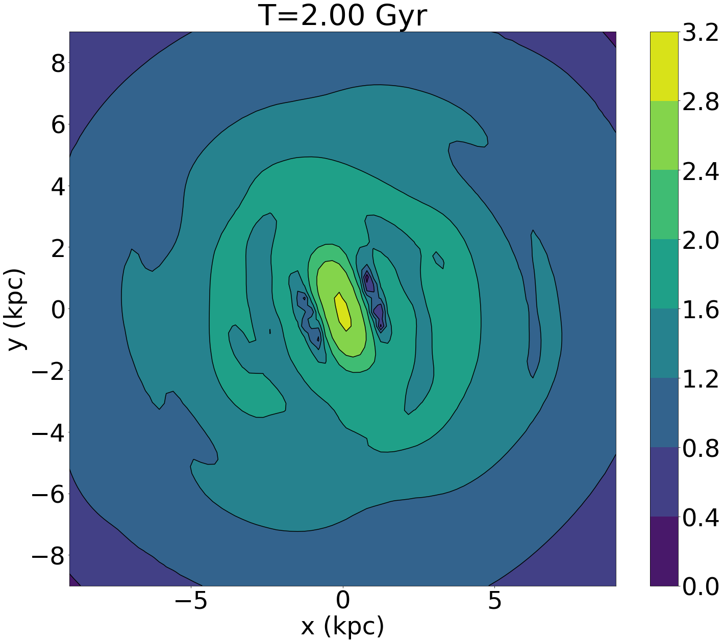
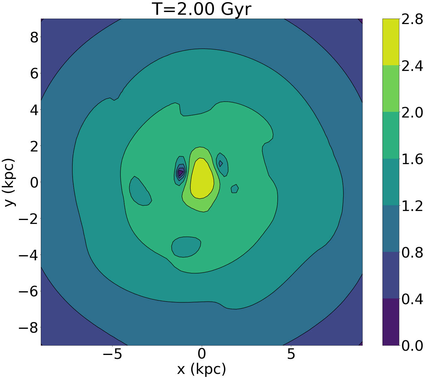
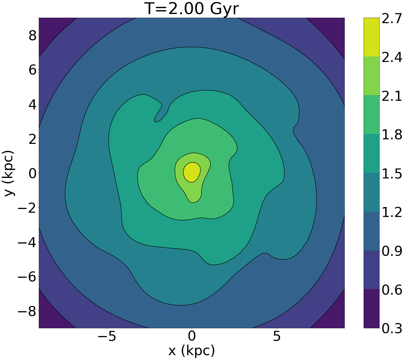
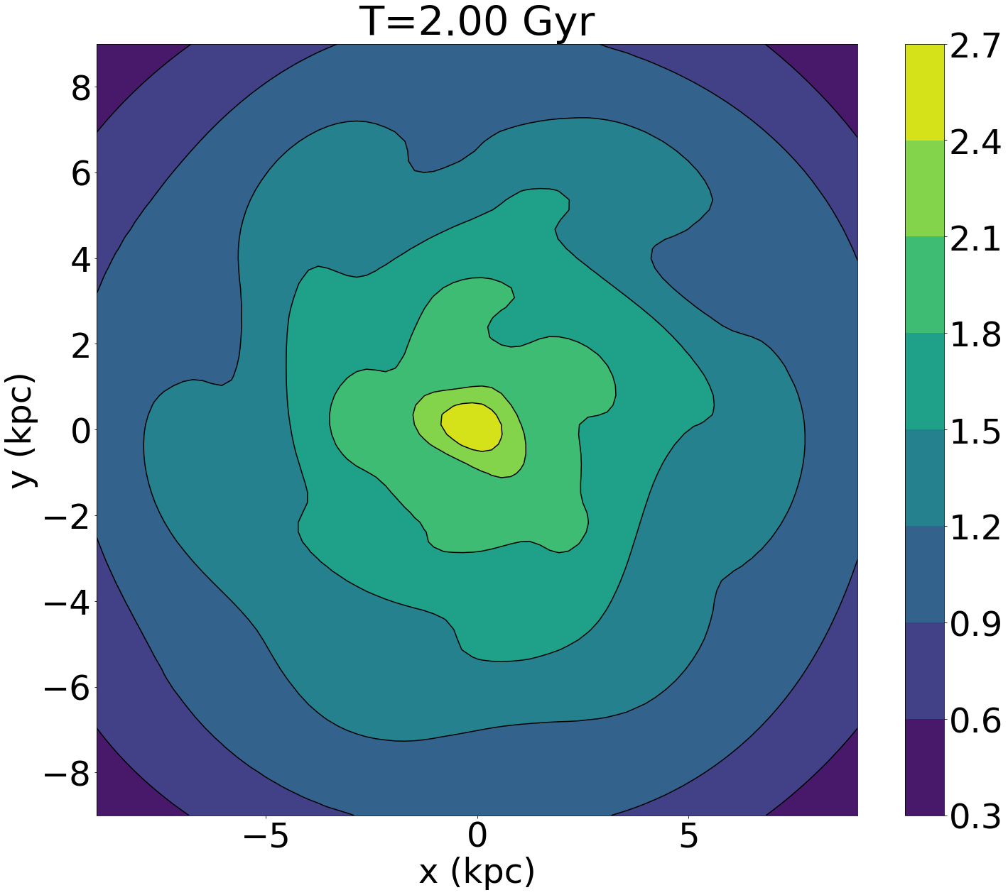
Figure 1: The disk surface density at $T=2{\rm\,Gyr}$. The upper-left panel shows the primary model with no SF feedback. The next three panels have SF feedback with $\epsilon=0.1$ and $\tau_{1}=20,40,80$ Myr and $\tau_{2}=\tau_{1}/2$, from left-to-right and top-to-bottom. The density scale is logarithmic in units of ${\rm\,M_{\odot}}/{\rm\,pc}^{2}$.

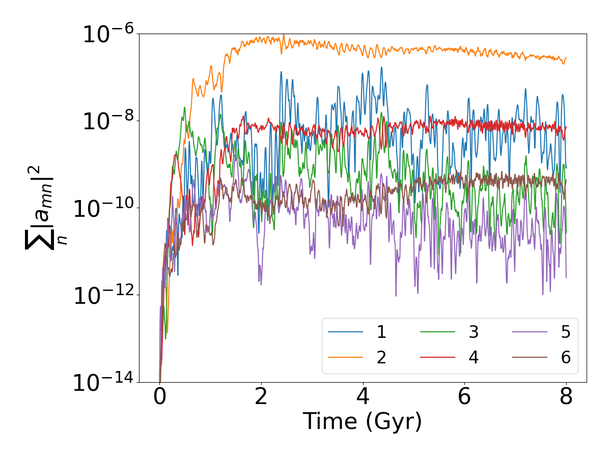
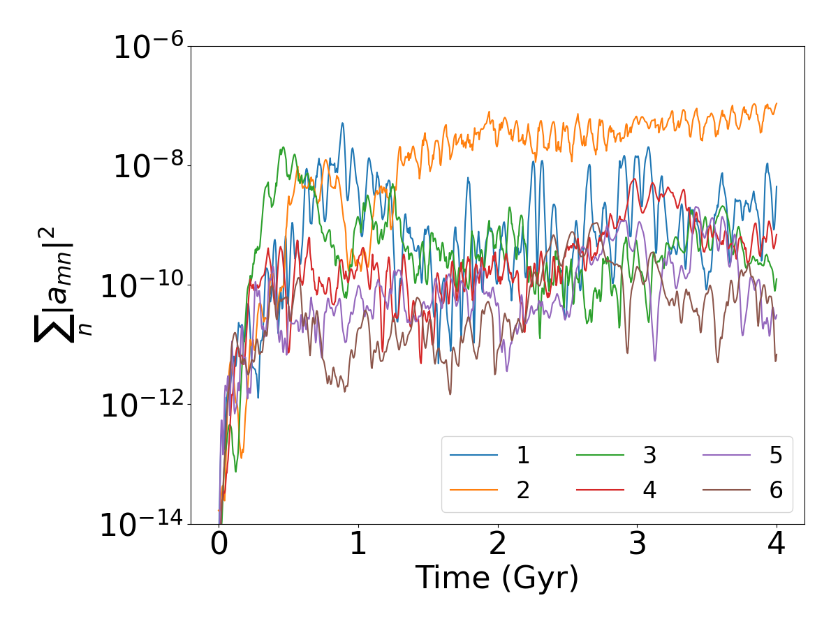
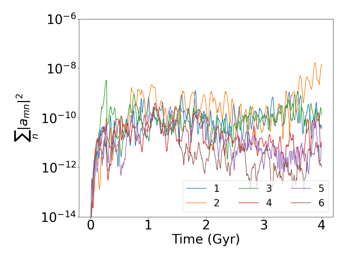
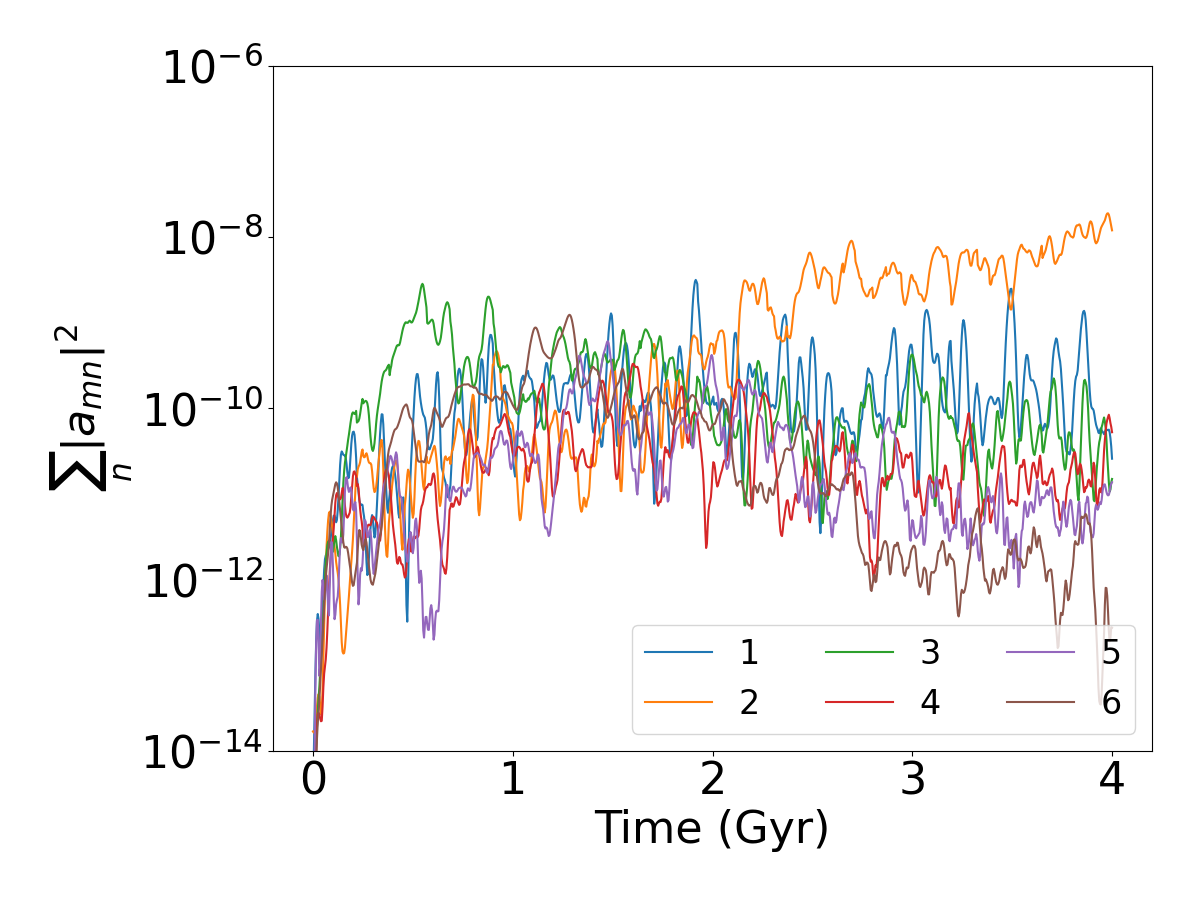
Figure 2: The gravitational power for azimuthal harmonics $m=1,\ldots,6$ (see inset legends) for each of the four runs from Fig. 1. The power had units of virial energy, $GM_{vir}^{2}/R_{vir}$. The $m=5,6$ harmonics have very little correlated power and are a good indicator of the particle noise floor.

3 Results

We begin in Section 3.1 with a summary demonstration of the consequences to bar formation with a series of 4 runs with successively more SF feedback. We compare this to bar formation with no SF feedback in Section 3.2. Later sections describe the sensitivity of the bar interaction to the time scale and amplitude of the SF feedback process. We end, in Section 3.3.4 with insight from the BarHMF model.

3.1 SF feedback: a quick demonstration

For this initial demonstration we consider four runs of the primary model: the first run has no SF, the second three fix $\epsilon=0.1$ with $\tau_{1}=20,40,80{\rm\,Myr}$ from the feedback prescription described in Section 2.4. The results are compared in Figure 1. We adopt $\tau_{2}=\tau_{1}/2$ in equations (6) and (7) which allows the disk to reaccrete its lost mass on a time scale shorter than the average interval between star-formation events. We have tried other choices, such as $\tau_{2}=\tau_{1}/4$ and $\tau_{2}=\tau_{1}$ and the results are qualitatively unchanged. The key dynamical effect is the decorrelation of the orbital precession that is induced by star-formation feedback prescription.

The strength of the non-axisymmetric features are nicely described by total power in each azimuthal harmonic $m$. The biorthogonal functions used in the BFE potential solver naturally describe this power. Specifically, the sum of the moduli for all coefficients with a particular value of $m$ is the total power in the gravitational field at harmonic order $m$. The square root of the power measures the mean amplitude of the gravitational potential in the BFE (Petersen et al., 2022). Figure 2 show the traces of the power for each of the non-axisymmetric orders $m\in[1,6]$ for the runs described in Figure 1. In the case without SF feedback (upper-left panel of Fig. 2), we clearly see coherent signal at all of the even harmonics $m$ with the amplitude of $m=4$ about 0.1 of $m=2$. The $m=4$ is responsible for the bar’s boxiness. Both dynamics of the bar and the natural modes in the dark-matter halo cause $m=1$ distortions. These are tend to fluctuate but have similar amplitude to the $m=4$ signal. Upon including SF feedback, the bar growth is strongly suppressed for all three values of $\tau_{1}$. The $\tau_{1}=20,80{\rm\,Myr}$ cases reveal some hint of an $m=2$ bar-like feature but comparison with the no SF feedback run reveals that these are down by an order of magnitude from the no feedback run (upper-left panel). The $\tau_{1}=40{\rm\,Myr}$ case has no obvious bar. The minimum at $\tau_{1}=40{\rm\,Myr}$ is naturally explained by increased coupling between the Markov jump process and the orbital frequencies necessary to support the bar. We will demonstrate this further in Section 3.3.4.

3.2 Evolution without SF feedback

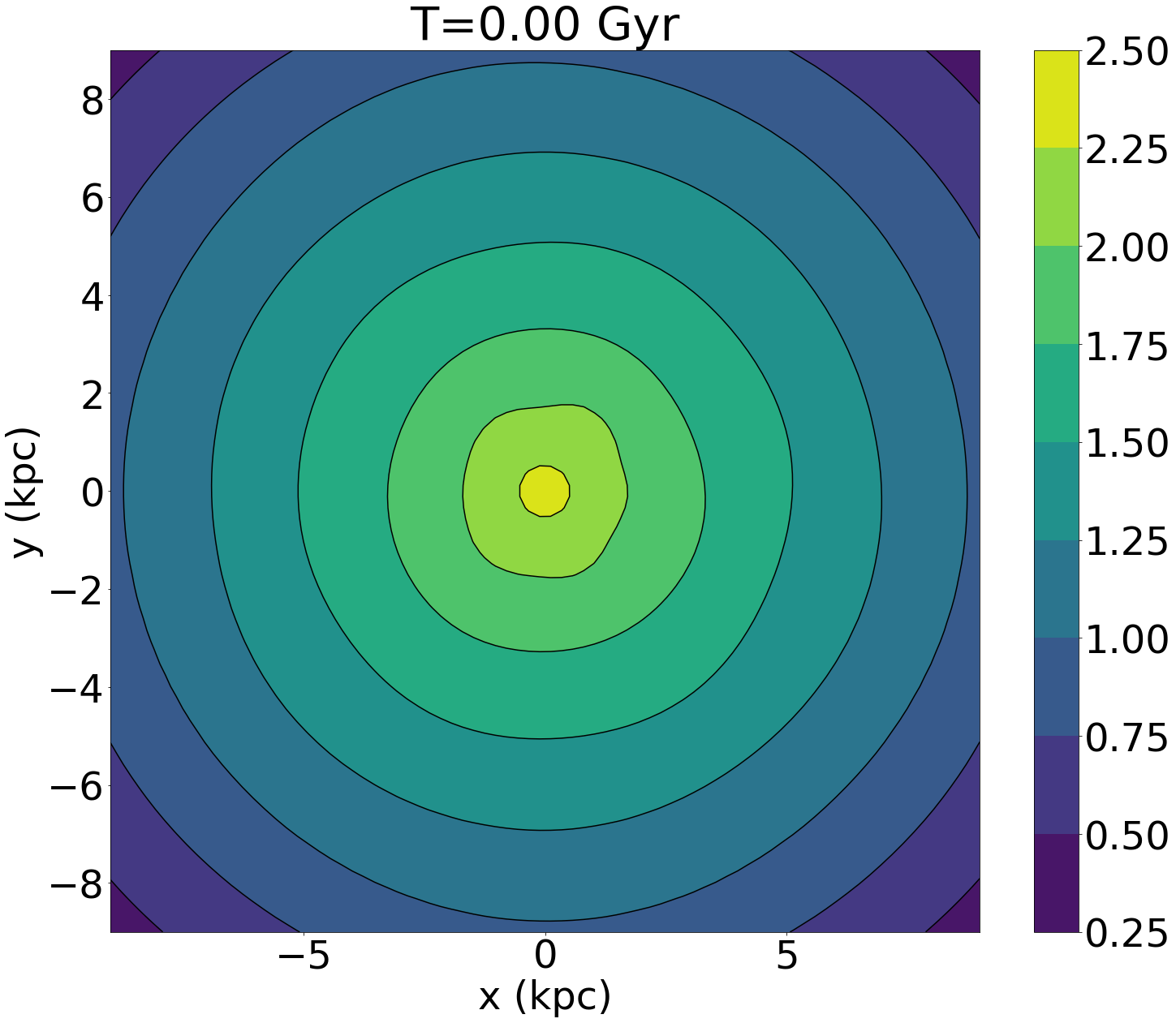
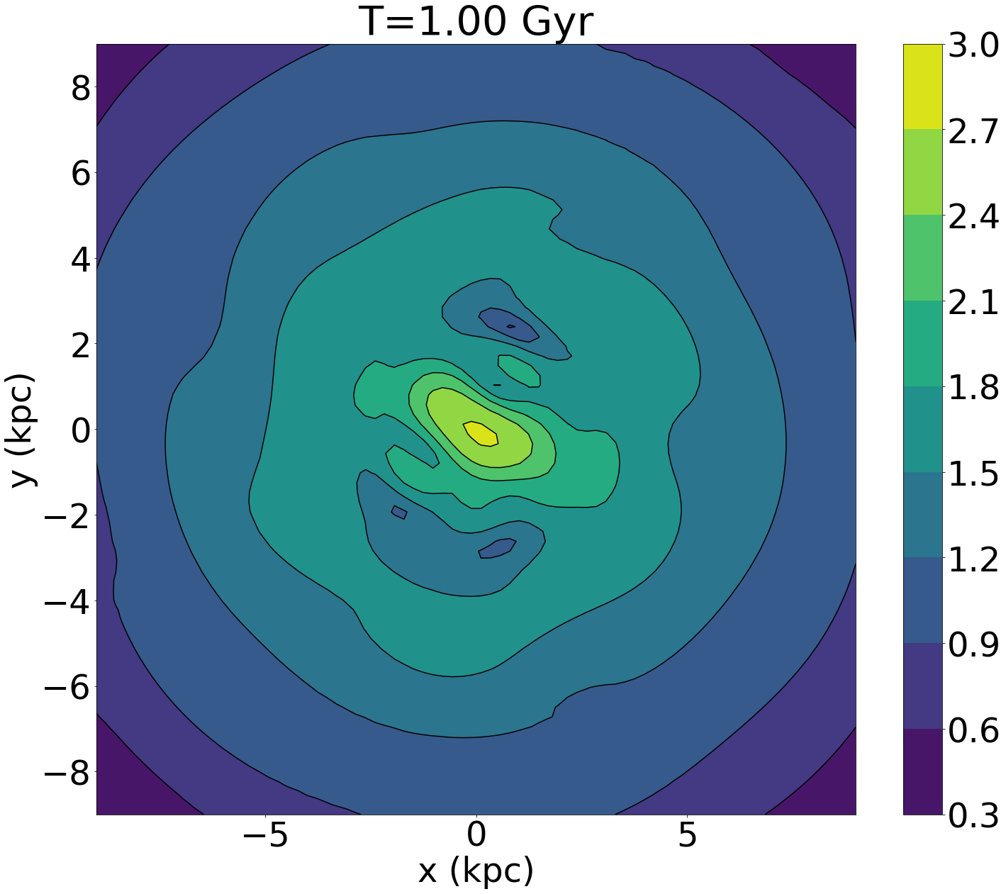
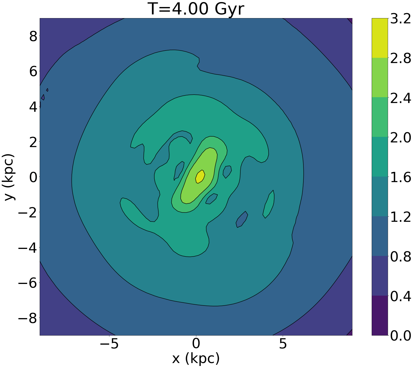
Figure 3: The surface density for the primary model with no SF feedback ($\epsilon=0$) at T=0, 1, 2, 4 Gyr. The bar reaches steady state by $T=2{\rm\,Gyr}$. The density scale is logarithmic in units of ${\rm\,M_{\odot}}/{\rm\,pc}^{2}$.

For comparison, we present a brief description of full N-body evolution using the primary model from Section 2.1 without the star-formation feedback prescription. This provides a reference for comparing the bar growth and evolution to simulations with feedback. The salient features of the evolution without feedback are as follows:

1. The growing bar becomes distinct at $T\approx 600$ Myr.

2. The pattern speed slows quickly during formation as it grows in strength and lengthens.

3. The bar reaches an approximate steady-state at $T\approx 2$ Gyr. The bar pattern speed decays slowly and nearly linearly thereafter.

Figure 3 shows the surface density at the start and at $T=1,2,4$ Gyr. The first panel shows the initial conditions reconstructed from the BFE. The second panel shows the bar at the of its growth phase. The bar is very slowly evolving in third and fourth panels. The rotation curve for the initial model (Fig. 4) shows the classic linearly rising inner profile that promotes bar growth following the Lynden-Bell condition (eq. 9).

Figure 5 describes the pattern speed, $\Omega_{p}$, which is computed from the complex phase of the first three radial terms in the $m=2$ part of the BFE. These first three terms contain 80% of the total $m=2$ power and accurately portray the shape and potential of the bar. The rapid change in $\Omega_{p}$ for $600{\rm\,Myr}\mathrel{\hbox{\hbox to0.0pt{\hbox{\lower 4.0pt\hbox{$\sim$}}\hss}\hbox{$<$}}}T\mathrel{\hbox{\hbox to0.0pt{\hbox{\lower 4.0pt\hbox{$\sim$}}\hss}\hbox{$<$}}}2{\rm\,Gyr}$ corresponds to the rapid growth in $m=2$ power. In most of this discussion, we will only consider evolution up to $T=4$ Gyr given our cosmic noon perspective; we show the power in the first panel of Figure 2 and pattern speed in Figure 5 up to $T=8$ Gyr for completeness. This run of pattern speed with time compares well with the primary run from Petersen et al. (2019) providing a check for the two-dimensional basis functions described in Section 2.2 and Appendix A.

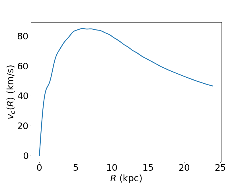
Figure 4: The circular velocity curve for the unperturbed halo and disk model described in Section 2.1.2 computed from the radial force in the simulation at $T=0$. The curve is approximately linearly increasing in the first scale length, $R=3{\rm\,kpc}$, with a peak at $R\approx 5{\rm\,kpc}$ and a slow decline thereafter.

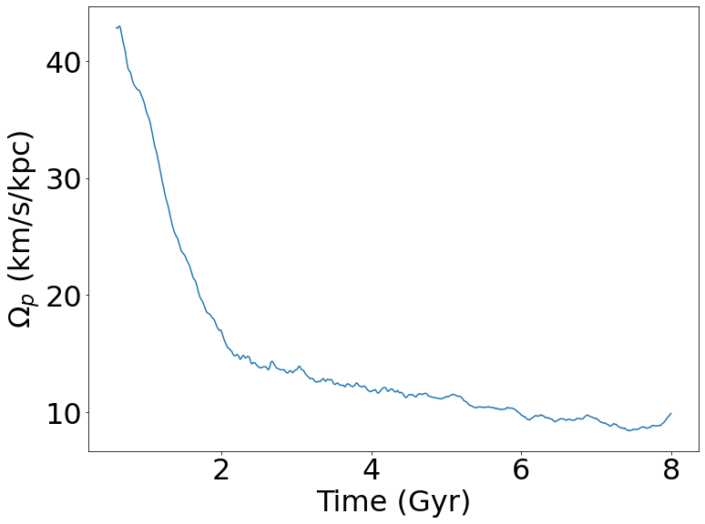
Figure 5: Bar pattern speed for the primary run shown from the point of bar assembly onward.

3.3 Sensitivity to the details of SF feedback

We quantify the variation of the response with the parameters of the feedback process by considering two distinct scenarios:

1. Fixed $\tau_{1}=20{\rm\,Myr}$ and varying amplitude of the mass loss, $\epsilon$ in Section 3.3.1.

2. Fixed $\epsilon=0.3$ and varying the value of $\tau_{1}$ in Section 3.3.2.

3.3.1 Comparison of frequencies

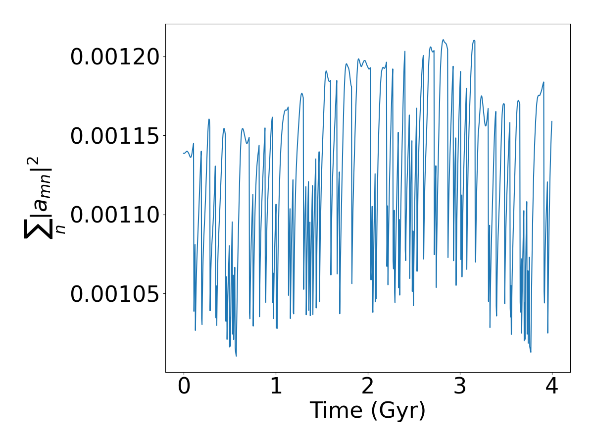
Figure 6: The run of $m=0$ power for the $\epsilon=0.1$, $\tau_{1}=40$ Myr simulation to illustrate the fluctuation in the gravitational power induced by star formation events. See Fig. 2 for an illustration of the non-axisymmetric power in the same simulation.

We fix $\epsilon=0.1$; equation (8) implies that the mass that temporarily leaves the disk per SF event is 1.4% of the total disk mass ($7\times 10^{7}{\rm\,M_{\odot}}$). In our stochastic model, $\tau_{1}$ is the average time between star-formation events; we explore $\tau_{1}\in[20,40,80]{\rm\,Myr}$, typical of measured star-formation events. It is the fluctuation of star formation activity and not the full scope of the overall starburst phase that is relevant here (see McQuinn et al. 2009 for discussion). We are envisioning repeated episodes of star formation in groups of giant molecular clouds that flicker over a Gyr time scale. The model itself only depends on the values of $\epsilon$ and $\tau$ so this is a characterization only.

The $m=0$ component represents most of the gravitational power in the disk and is not shown in Figure 2 to emphasize the non-axisymmetric features. We illustrate the effect of star-formation feedback on the gravitational power of the $m=0$ component alone in Figure 6 for the $\tau_{1}=40{\rm\,Myr}$ run. The value $\epsilon=0.1$ affects the total gravitational potential energy of the disk at a level of approximately 0.8%.

3.3.2 Comparison of amplitudes

Next, we fix $\tau_{1}=20{\rm\,Myr}$ and examine the variance with $\epsilon\in[0.1,0.3,0.5]$. Equation (8) implies that the mass lost per SF event for these values of $\epsilon$ are 1%, 4%, and 7%, respectively. These results are summarized and compared with results from previous section in Figure 7. This figure shows the ratio of the BFE amplitudes (root power) at $m=2$ for the runs with the star formation prescription for the chosen values of $\tau_{1}$ and $\epsilon$ with those from the primary model without feedback at $T=1,\,2,\,4{\rm\,Gyr}$. As expected, the lower panel shows that larger values of mass loss, $\epsilon$, lead to smaller amplitude ratios at all times. The upper panel summarizes the results from the previous section with an extended range of $\tau 1$ from 10–500 Myr: the largest damage is done to the bar instability for $\tau_{1}\approx 50{\rm\,Myr}$. This time interval is close to the characteristic orbital time for inner bar orbits. As $\tau_{1}$ increases, the amplitude ratio increases. However, even for large value of $\tau_{1}=500{\rm\,Myr}$, the bar amplitude is suppressed by a factor of two. To index the amplitude ratio to bar morphology, the second panel from Figure 1 is an amplitude ratio of 0.23. The next two panels are ratios of 0.13 and 0.03. The 0.23 case (second panel) is typical of a weak bar; ratios below $\sim 0.2)$ (third and fourth panels) are not bar-like.

We chose the value of $\epsilon=0.1$ used in Section 3.3.2 to be close to the critical threshold for significant suppression of the bar formation. For the larger value of $\epsilon=0.3$, the amplitude ratios for various values of $\tau_{1}$ are shown in Figure 8. The overall values of the suppression ratios are smaller, as expected, and the sensitivity to value of $\tau_{1}$ are much weaker.

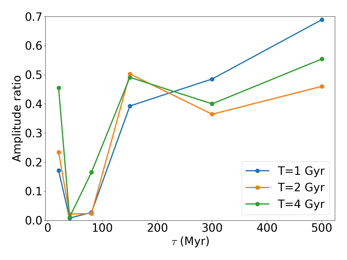
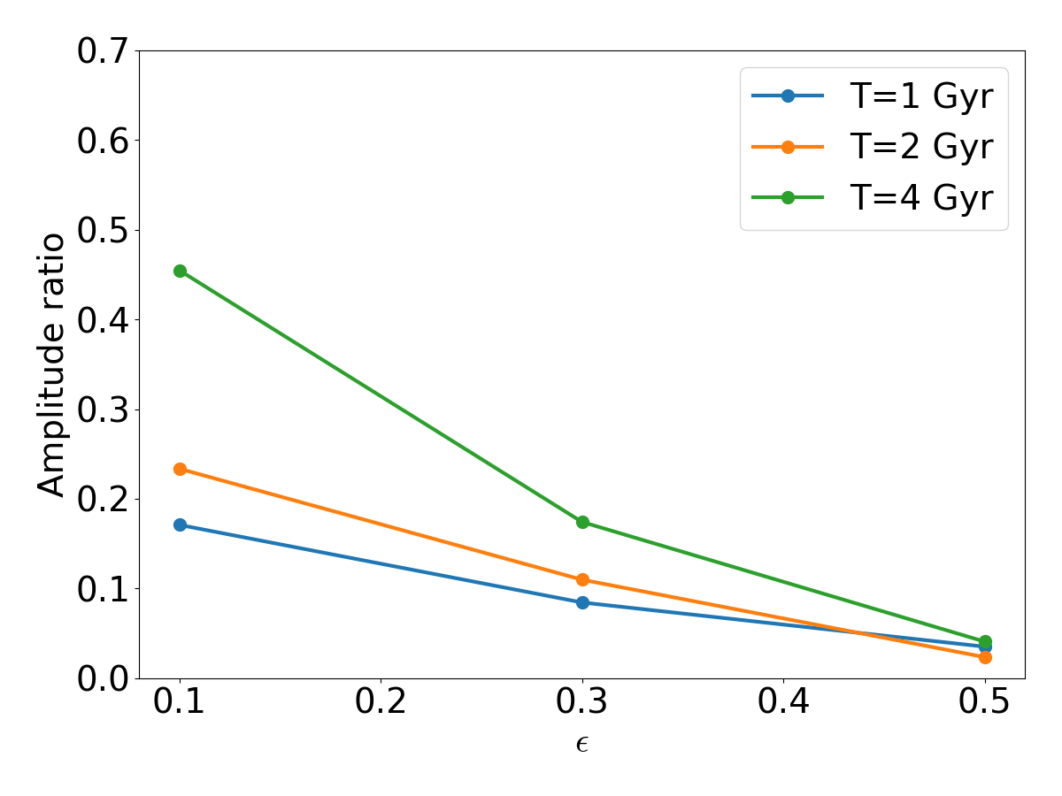
Figure 7: The ratio of the $m=2$ amplitudes at $T=0.5,1.0,2.0$ in simulations with SF feedback to the $m=2$ amplitude from the primary simulation without SF feedback. Top: constant value of $\epsilon=0.1$ with values of $\tau_{1}$ along the x-axis. Bottom: constant value of $\tau_{1}=0.01$ with values of $\epsilon$ along the x-axis.

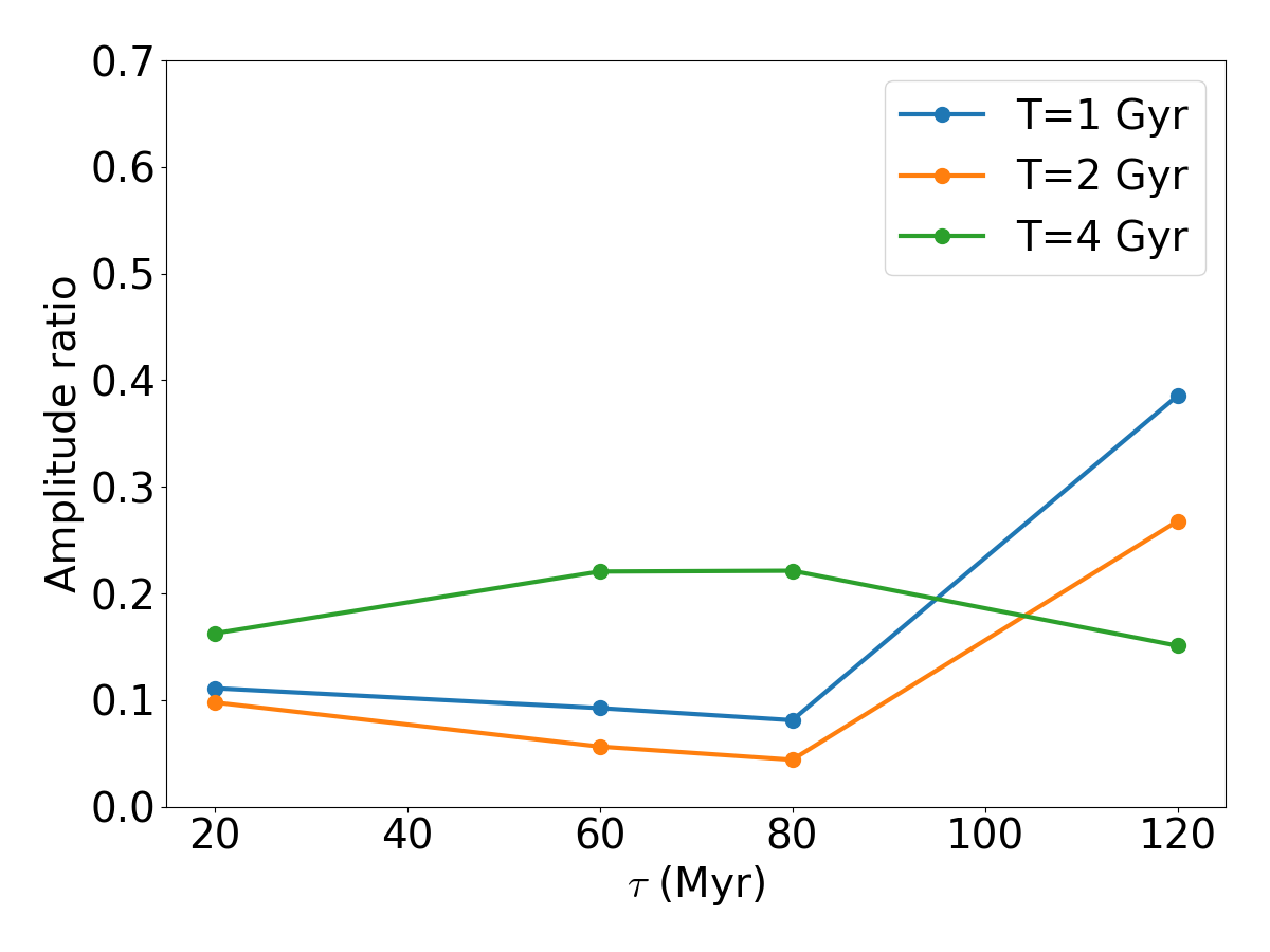
Figure 8: As in the top panel of Fig. 7 but for $\epsilon=0.3$. Here, the suppression ratios are smaller overall with less variation in $\tau_{1}$.

3.3.3 The effect of SF feedback on a preexisting bar

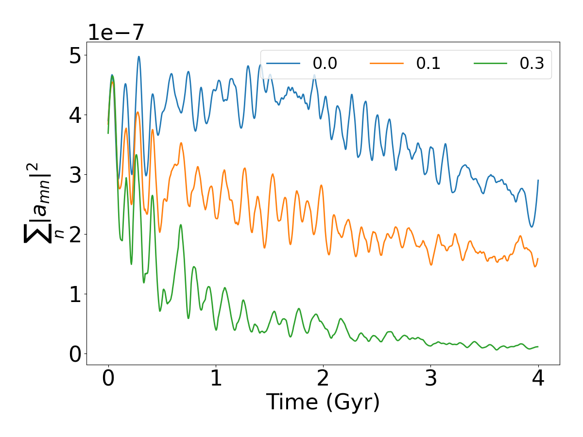
Figure 9: The primary model is evolved without SF feedback until $T=2{\rm\,Gyr}$ and then subjected to SF feedback. This figure shows the $m=2$ power after SF feedback commences for various amplitudes, $\epsilon$. The run with $\epsilon=0.0$ has no SF feedback, for comparison. A model with $\epsilon=0.1$ reduces the bar amplitude by a factor of 2 and the model with $\epsilon=0.3$ eliminates the bar after 2 Gyr.

Bar formation in an otherwise quiescent galaxy could be the source of gas advection that induces a central star burst. We ask whether our Markov-process SF feedback model can be used to destroy a preexisting bar? We begin with the phase space from the primary N-body simulation without SF feedback at $T=2{\rm\,Gyr}$ shown in Figure 3. We then apply the stochastic model with two different feedback strengths, $\epsilon=0.1,0.3$. We set $\tau_{1}=20{\rm\,Myr}$ with $\tau_{2}=\tau_{1}/2$ as in previous cases. For $\epsilon=0.1$, the feedback diminishes the bar amplitude by a factor of 2; the bar reaches a new steady-state amplitude in approximately 4 Gyr. For $\epsilon=0.3$, the bar is destroyed after 2 Gyr. Some $m=2$ power remains in the form of an oval distortion at larger radii than the original bar.

In summary, the SF feedback model can be used to destroy an existing bar. More feedback amplitude is required to destroy it than to prevent it owing to the extra self-gravity in the bar itself. This calls in to question our expectation that bar are eternal once formed, especially in the formation epoch. We suggest exploring this scenario using existing suites of cosmological galaxy formation simulations that include feedback. Barred galaxies are ubiquitous in simulations of isolated galaxies at the present epoch although it is clear observationally that not all disk galaxies have bars. It has been argued that central mass concentrations may be sufficient to destroy bars althoug there is some numerical evidence to the contrary (Athanassoula et al., 2005). The feedback model proposed here provides another possible bar destruction mechanism.

3.3.4 Insight from perturbation theory

Section 2.5 and Appendix B describes a simulation method tailored to the dynamics of Lynden-Bell’s mechanism specifically. In essence, each simulation particle contributes its part to the ensemble action-angle expansion of gravitational potential restricted to the same commensurate term considered by Lynden-Bell (1979). Given that this model is a cousin of the classical cosine HMF ring model (Antoni and Ruffo, 1995) specialized to the interaction implied by the Lynden-Bell mechanism, we find the term BarHMF to be an apt descriptor. Although the model employs an interaction potential from linear theory, it is a non-linear model. Indeed, Appendix B demonstrates that many of the basic results of bar formation and growth from full N-body simulations are found in the BarHMF model. For example, the BarHMF model reproduces the non-linear saturation of the bar amplitude with a growth rate proportional to disk mass.

The perturbation scheme outlined in Section 2.4 is applied to the BarHMF simulation as follows. The axisymmetric component of the gravitational potential is represented by a spherical monopole for computational convenience. In other words, the disk does not have its own $m=0$ self gravity but does have $m=2$ self gravity. The Markov-process SF feedback model changes the central mass through equation (6) and causes fluctuations in the monopole that affect the BarHMF dynamics. A feedback event implies in an overall decrease in central mass according to Step 2 in the algorithm from Section 2.4. This mass change is applied suddenly as in the full N-body simulation. This increases the energy of the BarHMF particles by $\delta E=GM_{d}\epsilon/(\mu\lambda a)$ where $\mu$ parametrizes the change in gravitational potential caused by the SF-induced mass loss. We choose $r_{g}\equiv\mu\lambda a$ to be the gravitational radius of the monopole contribution of the total gravitational energy from change in disk mass inside of $\lambda a$. For a spherical model, $r_{g}$ is approximately $0.4$ times the half-mass radius of the disk mass enclosed by $\lambda a$ (Binney and Tremaine, 2008) and determines $\mu$. This approximation most likely underestimates the effect on the disk for a given $\epsilon$ but is consistent with the assumptions in our BarHMF application.

The main difference between the SF model for BarHMF and the full exp model is that both the change in energy and recovery time is instantaneous for BarHMF and only the change in energy is instantaneous for the exp model. This is consistent with the time averaging implicit in the BarHMF contribution to the interaction potential: the decay time $\tau_{2}$ from equation (7) is shorter than the orbital time and therefore instantaneous in the time-averaged Hamiltonian context.

As described in Appendix B, the BarHMF particles interact with each other. For particles with the same actions, the coupling depends on the precession angles of their apsides relative to the bar position angle in some rotating frame with $\Omega_{p}$. The precession frequency is small compared to the mean orbital frequency for orbits comprising the bar. For example, the perfect bar supporting trajectory has zero precession frequency with respect to the bar major axis. For a slightly imperfect bar supporting trajectory, the angle of apsides will precess slowly relative to the bar pattern. For this reason, the action conjugate to the precession angle is called the slow action and is proportional to the angular momentum. The precession angle itself is called the slow angle. There is a second degree of freedom whose frequency is proportional to the orbital frequencies and therefore faster than the precession frequency. The BarHMF particles result from an average over this fast degree of freedom leaving only one active slow degree-of-freedom. Without any external perturbations, the fast action is conserved for all time. A SF event causes a sudden change in energy and radial action. This fluctuation is axisymmetric, conserving the angular momentum of stellar trajectories; therefore the slow action remains unchanged. However, the fast action is a linear combination of the radial action and angular momentum. The fast action changes as result of the energy causing a jump in radial action.

If these jumps in fast action are sufficiently large, a BarHMF particle which had been librating about the about the bar position can find itself precessing away from the bar. This causes the bar to grow more slowly, decay, or not grow at all. We illustrate the dynamics in a simple case of two BarHMF particles at one disk scale length orbiting in the truncated NFW-like model (eq. 2). Each trajectory feels a change in energy from a SF event every $\tau_{1}=20{\rm\,Myr}$. Each event removes $2\times 10^{8}{\rm\,M_{\odot}}$ from the inner 20% of the disk scale length ($600{\rm\,pc}$ for the Milky Way). We assume that this quickly cools back on the disk maintaining a steady state potential punctuated by instantaneous changes in the radial action. Figure 10 shows two BarHMF runs that differ only in their initial $\Delta w_{s}$: the first of these runs begins with $\Delta w_{s}=0.02$ (or $\approx 1^{\circ}$ shown in blue) and the second begins with $\Delta w_{s}=1.0$ (or $\approx 57^{\circ}$ shown in orange). The first run undergoes significant jumps in $\Delta w_{s}$ but remains in libration. The jumps in the second with larger libration amplitude are enough to push the trajectory from libration into rotation. The dashed curves depict the same trajectories without perturbation and can be compared to the two-particle BarHMF runs from Appendix B in Figure 14.

Figures 11 shows the BarHMF model described in Appendix B for the NFW-like background model that is generally bar promoting. Each of these simulations has $N=1000$ particles and uses $\tau_{1}=20{\rm\,Myr}$. The legend describes the mass loss per SF in solar masses scaled to Milky Way units for familiarity. For no SF at all, the bar exponential grows in approximately 2 Gyr before leveling off into a steady state. Recall that there is no coupling between the bar and disk or halo so the bar can not slow. For $4\times 10^{7}{\rm\,M_{\odot}}$ per event, the bar grows more slowly then levels off and begins to decay. The overall saturation amplitude is a factor of 5 smaller than with no SF at all. For a mass loss of $2\times 10^{8}{\rm\,M_{\odot}}$ per event, the bar grows but very slowly, reaching only 10% of its saturation amplitude in Figure 2 at $T=4{\rm\,Gyr}$. For larger mass loss events, the bar can not grow at all.

The thresholds in $\epsilon$ appear to be larger here than for the full simulation. This may have a number of causes. First, this may be an artifact of the spherical background model and the gravitational radius approximation. The work done on the spherical potential from the feedback is likely to be relatively smaller in effect for the spherical monopole than for the flat axisymmetric disk. Secondly, the initial actions are chosen for a fixed eccentricity with guiding centers in a narrow ring as described in Appendix B. The resulting dynamics will differ from the full simulation that has a disk with an astronomically motivated exponential distribution. We have chosen the total mass of the BarHMF particles to approximate the mass of the exponential disk between pericenter and apocenter, but we do not expect a one-to-one correspondence with full N-body simulations. Nonetheless, the qualitative trends are similar which suggest that the BarHMF dynamics represents the main features of the underlying mechanism.

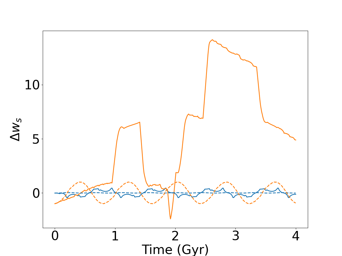
Figure 10: Change in relative precession angle, $\Delta w_{s}$, for a two-particle BarHMF simulation with SF feedback. The SF events, which occur every 20 million years push $2\times 10^{8}{\rm\,M_{\odot}}$ into the inner halo. We assume that this quickly cools back on the disk maintaining a steady state. The sudden change in gravitational potential changes the fast action for each trajectory. The two runs differ only in their initial $\Delta w_{s}$ with 0.02 rad (blue) and 1.0 rad (orange). The dashed curves show the run of $\Delta w_{s}$ without feedback.

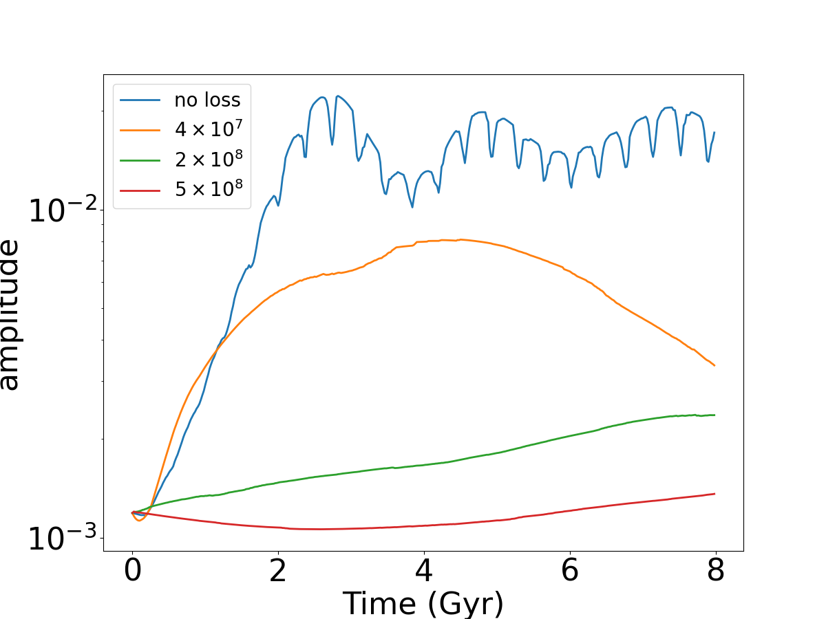
Figure 11: Bar growth as a function of mass loss per event (in ${\rm\,M_{\odot}}$) for the BarHMF in Milky Way units of $10^{12}{\rm\,M_{\odot}}$ for easy comparison. The event frequency is $\tau=20{\rm\,Myr}$.

4 Conclusions

We investigate the dynamical importance of feedback-induced gravitational fluctuations on the bar instability using a Markov jump-process model; intervals between feedback events are random draws from a Poisson distribution. We began with a full N-body simulation of a galactic disk in a live dark-matter halo with a mass typical of a disk at $z\sim 2.5$ which is roughly a factor of four lower than at $z=0$. Our primary, unperturbed model forms a stable bar in approximately 1 Gyr. We model the gravitational influence of star-formation feedback by perturbing that simulation with a stochastic mass-loss process which removes a small fraction $\epsilon$ of mass in the inner disk at a characteristic time $\tau_{1}$. The mass is lost from the inner 2/3 of the disk scale length or 2 kpc in Milky-Way units, causing a gravitational fluctuation in energy. The lost mass is assumed to resettle on the disk at another characteristic time $\tau_{2}$. We choose $\tau_{2}\mathrel{\hbox{\hbox to0.0pt{\hbox{\lower 4.0pt\hbox{$\sim$}}\hss}\hbox{$<$}}}\tau_{1}$ typical of the star-formation event frequency: between 20 and 100 Myr. We parametrize the mass-loss strength as the fraction of the disk mass in the inner 2/3 of the disk scale length in the resulting outflow. The amplitude of the mass loss ranges from 1% to 7% of the total disk mass, typical of strong stellar feedback at cosmic noon. The process itself is designed to capture the temporal features of gravitational fluctuations from feedback; we intend for ranges in amplitude, $\epsilon$, and time scales, $\tau_{1}$ and $\tau_{2}$, (Fig. 7) to be compared to detailed physical models.

To gain physical insight into the dynamical nature of the coupling between star-formation feedback and the bar instability, we developed a novel one-degree-of-freedom simulation based on the classical bar instability from linear perturbation theory (Lynden-Bell, 1979). Each particle in the simulation interacts with the bulk of particle ensemble through the quadrupole force exerted near resonance. In other words, each particle is dumbbell-shaped in space with two actions characterizing its radial extend and spread. The one degree of freedom is its azimuthal orientation. This specialized simulation reproduces all of the major features the bar instability in the full N-body simulation including non-linear saturation of the exponential growth (see Appendix B).

We may use this model to understand the dynamics of coupling. In the absence of SF feedback, only the net angular momentum of stellar orbits change through resonant interaction. A particular linear combination of the radial action and angular momentum remains invariant. The bar begins with the chance positional alignment of some dumbbell orientations. Their collective gravity cause more dumbbells to align, driving an exponential instability. However, the fluctuations in the gravitational potential induced by star-formation process affects the previously invariants, by changing the radial action. These fluctuations disturb the libration of particles in the quadrupole of the bulk, slowing or eliminating the bar instability depending on the strength of the SF feedback.

The key findings are as follows:

1. Mass-loss fractions of $\epsilon\geq 0.1$ in the inner few kiloparsecs of a disk are enough to dramatically affect the bar formation. These result in bar amplitude that are at most 50% of the unperturbed case.

2. We demonstrate that fluctuations in the gravitational potential of the inner galaxy couple to the radial action of orbits in the bar instability. These fluctuations reduce or eliminate the bar instability, consistent with the results of the full N-body simulation. This simple model provides a way of predicting the importance of SF feedback to disk instabilities.

3. The rate of star-formation feedback matters. The bar amplitude is reduced by an order of magnitude (and some cases suppressed altogether) if $\tau_{1}$ roughly matches the typical orbital period. This makes good dynamical sense. If disk orbits respond to the self-gravity of a quadrupole by precessing towards the potential well of the quadrupole, the bar amplitude will grow. However, if this precession is disrupted by changes in the underlying potential, this growth is reduced or eliminated.

4. For large amplitude mass loss events, e.g. closer to our upper limit of 7% mass changes per event, the amplitude of bar growth is suppressed independent of $\tau_{1}$.

5. The bars that do form in the presence of significant SF-induced fluctuations are poorly organized in a qualitative sense. They tend to shed mass and lose stability as star-formation events continue.

Our overall focus is the mechanism that connects the stochastic nature of galaxy feedback mechanisms with the smooth orbital motion of classical galaxy dynamics. As in dynamics generally, the key important quantities are frequencies. A stochastic process can be characterized by its autocorrelation function, and here, the process is Poisson, with a characteristic frequency $\sim 1/\tau_{1}$. The coincidence $\tau_{1}\sim\tau_{dyn}$ suggests the possibility of interesting coupling. The importance of this coupling to the overall dynamics of the bar instability depends on the details and requires explicit calculation. To that end, we provide evidence for its magnitude and importance by a combination of direct N-body simulation and a idealized simulation restricted to the dynamics of bar instability specifically. The similarity of the behavior in the two calculations suggests that we have successfully described the mechanism.

We emphasize that the details of the feedback process have been greatly simplified in this study. For example, we have assumed pure axisymmetric central fluctuations, ignoring non-axisymmetric dependence. Rather, we have chosen to explore the two important parameters of the simplest possible stochastic model that excites gravitational fluctuations–an amplitude and characteristic frequency–and provide predictions for range of those quantities necessary to have impact on the bar formation. Motivated by rough estimates from more detailed observational and theoretical studies, we find that range of these parameters overlap predicted ranges, at least during the epoch of peak star formation. The expected diversity of galaxy formation conditions suggest that the coupling between feedback and bar formation will not be binary; some systems may still be able to easily form bars at early epochs and others not. Moreover, we have demonstrated that strong feedback coupling may be capable of eroding and even destroying a bar after formation.

Appendix A Two-dimensional disk bases

The latest version of exp includes two-dimensional cylindrical disk bases with three-dimensional gravitational fields. This allows for gravitational couples between two- and three-dimensional components. These bases are used for the simulations in Section 3 that include the coupling to the dark-matter halo. For completeness, this section describes the construction and computation of the two-dimensional cylindrical bases as used by exp.

We construct two-dimensional polar bases using the same empirical orthogonal function (EOF) technique used to compute the three dimensional cylindrical basis (Petersen et al., 2022). In essence, we compute the Gram matrix whose entries are the inner product of an input basis weighted by the density of the desired equilibrium profile. The new basis functions are the input basis weighted by each of the eigenvectors of the Gram matrix. The construction provides a basis conditioned by the target equilibrium galaxy profile. The user has the choice of two possible two-dimensional input bases:

1. The cylindrical Bessel functions of the first kind, $J_{m}(\alpha_{m,n}R/R_{max})$ where $\alpha_{m,n}$ is the $n^{th}$ root of $J_{m}$ and $R_{max}$ is an outer boundary. Thus, orthogonality is defined over a finite domain by construction.

2. The Clutton-Brock two-dimensional basis (Clutton-Brock, 1972) which orthogonal over the semi-infinite domain.

The user then chooses a conditioning density. Currently, these are the exponential disk, the Kuzmin (Toomre) disk, the finite Mestel disk (Binney and Tremaine, 2008), the tapered Mestel or Zang disk (Zang, 1976). The code was written to allow for a user-defined density function and this will be available in a future release of exp.

The coupling between the two-dimensional disk and other three-dimensional components (e.g. a dark-matter halo or a bulge) requires evaluating the gravitational potential and its gradient everywhere in space. The three-dimensional gravitational potential is not automatically computed by the two-dimensional recursion relations that define the biorthogonal functions but can be evaluated by Hankel transform. Numerically, this can be done very accurately over a finite domain with the quasi-discrete Hankel transformation (QDHT, Yu et al., 1998; Guizar-Sicairos and Gutiérrez-Vega, 2004). The QDHT algorithm exploits special properties of the Bessel functions and is best suited for finite density profiles whose two-dimensional gravitational potential are well-described using the cylindrical Bessel basis. This is automatically true for the EOF bases derived from the cylindrical Bessel functions. For this reason, the Clutton-Brock basis should only be used for EOF basis construction for applications where the three-dimensional gravitational potential is not needed.

The in-plane density, potential and force fields are one-dimensional functions for each azimuthal order $m$ and radial order $n$. exp tables the EOF basis solutions on a fine grid and evaluates these with linear interpolation. This is numerically efficient and accurate. The potential and force fields for $|z|>0$ require two-dimensional tables. Similarly, exp finely-grids these functions in two-dimensional tables and evaluates them with bilinear interpolation.

The remainder of this section describes the implementation of the two-dimensional basis. We begin in Section A.1 with a summary of the QDHT algorithm followed by its application to the Hankel transform that defines two-dimensional biorthogonal basis functions in Section A.2. The complete algorithm is presented in Section A.3 followed by a discussion of the pros and cons of this approach in Section A.4.

A.1 A brief description of the QDHT algorithm

The development here follows Yu et al. (1998). The continuous Hankel transform pair is

$$g(k) = \int_{0}^{\infty}drrf(r)J_{\nu}(kr),$$

$$f(r) = \int_{0}^{\infty}dkkg(k)J_{\nu}(kr),$$ (10)

where $J_{\nu}$ is the Bessel function of the first kind of integer order $\nu$. The discrete Hankel transform may be obtained from equation (10) by imposing

$$g(k)=0 \qquad\mbox{for}\ k>K,$$

$$f(r)=0 \qquad\mbox{for}\ r>R.$$

Using this condition in equations (10) yields:

$$g(k) = \int_{0}^{R}drrf(r)J_{\nu}(kr),$$

$$f(r) = \int_{0}^{K}dkkg(k)J_{\nu}(kr).$$ (11)

We can now use the usual Fourier-Bessel expansion (Watson, 1941) to evaluate $f(r)$ as follows:

$$f(r)=\sum_{m=1}^{\infty}C_{\nu m}J_{\nu}\left(a_{\nu m}\frac{r}{R}\right)$$ (12)

for $0\leq r\leq R$ with

$$C_{\nu m}=\frac{2}{R^{2}J_{\nu+1}^{2}(a_{\nu m})}\int_{0}^{R}drrf(r)J_{\nu}\left(\alpha_{\nu m}\frac{r}{R}\right)$$ (13)

and $\alpha_{\nu m}$ is the $m^{\mbox{th}}$ root of $J_{\nu}$. Equation (13) is a direct application of the well-known orthogonality relation for Bessel functions of the first kind. By inspection, it is clear that:

$$C_{\nu m}=\frac{2}{R^{2}J_{\nu+1}^{2}(a_{\nu m})}g\left(\frac{\alpha_{\nu m}}{R}\right).$$ (14)

The continuous transform in equations (11) becomes a discrete transform by choosing the evaluation points for $r$ and $k$ as:

$$r_{j} =\frac{\alpha_{\nu j}}{K}$$

$$k_{j} =\frac{\alpha_{\nu j}}{R}.$$ (15)

Substituting into equation (12) and using equation (14), we get

$$f\left(\frac{\alpha_{\nu n}}{V}\right)=\sum_{m=1}^{\infty}\frac{2}{R^{2}J_{\nu+1}^{2}(a_{\nu m})}g\left(\frac{\alpha_{\nu m}}{R}\right)J_{\nu}\left(\frac{\alpha_{\nu m}\alpha_{\nu n}}{RK}\right)$$ (16)

and by symmetry

$$g\left(\frac{\alpha_{\nu m}}{R}\right)=\sum_{n=1}^{\infty}\frac{2}{K^{2}J_{\nu+1}^{2}(a_{\nu n})}f\left(\frac{\alpha_{\nu n}}{K}\right)J_{\nu}\left(\frac{\alpha_{\nu m}\alpha_{\nu n}}{RK}\right).$$ (17)

Truncating the upper limit of sum of the indices $m$ and $n$ to some value $N$ in equations (16) and (17) yields the discrete Hankel transform. The symmetry in the these two equations can be made manifest by defining further the two vectors with elements

$$F_{i} =\frac{f(\alpha_{\nu i}/K)R}{J_{\nu+1}(\alpha_{\nu i})}$$

$$G_{i} =\frac{g(\alpha_{\nu i}/R)K}{J_{\nu+1}(\alpha_{\nu i})}$$ (18)

and the matrix with elements

$$T_{ij}=\frac{2}{RKJ_{\nu+1}(a_{\nu i})J_{\nu+1}(a_{\nu j})}J_{\nu}\left(\frac{\alpha_{\nu m}\alpha_{\nu n}}{RK}\right).$$ (19)

Then, the discrete Hankel transform may be written in matrix notation as

$$\mathbf{G} =\mathbf{T}\cdot\mathbf{F},$$

$$\mathbf{F} =\mathbf{T}\cdot\mathbf{G}.$$ (20)

The transform is very accurate numerically, typically one part in $10^{8}$ in algorithm tests, when the target function is well-represented by a Bessel expansion,

A.2 Construction of a biorthgonal basis

Armed with the finite Hankel transform and an algorithm for its evaluation, we derive a two-dimensional biorthgonal basis using the eigenfunctions of the Laplacian described in Toomre (1963) and clearly summarized in §2.6.2 of Binney and Tremaine (2008). Specifically, gravitational potential functions in the form

$$\Phi_{m}(r,\phi;k)=e^{im\phi}J_{m}(kr)$$ (21)

have the surface density

$$\Sigma_{m}(r,\phi;k)=\frac{k}{2\pi G}e^{im\phi}J_{m}(kr)$$ (22)

Using the notation from the previous section, let

$$\Phi_{mj}(r,\phi) =D_{mj}e^{im\phi}J_{m}(\alpha_{mj}r/R),$$

$$\Sigma_{mj}(r,\phi) =(-1)^{m}\frac{\alpha_{mj}}{2\pi RG}D_{mj}e^{im\phi}J_{m}(\alpha_{mj}r/R),$$ (23)

where $D_{mj}$ is a normalization. Using the standard properties of Bessel functions, we may write:

$$\left(\Phi_{m^{\prime}j},\Sigma_{mk}\right) =\int_{0}^{2\pi}d\phi\int_{0}^{R}r^{2}\Phi_{m^{\prime}j}^{\ast}(r)\Sigma_{mk}(r)$$

$$=D_{mj}D_{mk}\frac{\alpha_{mj}}{RG}\int_{0}^{R}drr^{2}J_{m}(\alpha_{mj}r/R)J_{m}(\alpha_{mk}r/R)$$

$$=\frac{\alpha_{mj}}{2RG}\left(J_{m}(\alpha_{mj+1}\right)^{2}(D_{mj})^{2}\delta_{m^{\prime}m}\delta_{jk}.$$ (24)

Setting equation (24) equal to one defines the normalizing coefficient $D_{mj}$ in equations (23). Finally, we can use the EOF conditioning procedure described above and in Petersen et al. (2022) to obtain a new biorthogonal basis that best fits a desired equilibrium density model. This new basis is related to equations (23) by a linear transformation.

In the application needed here, we want to describe the gravitational potential for three dimensional space. We may use Toomre’s method (Toomre, 1963) to do this. For razor-thin disk with surface density $\Sigma(r,\phi)$, the gravitational potential is:

$$\Phi(r,\phi,z)=\sum_{m=-\infty}^{\infty}\int_{0}^{\infty}dkS_{m}(k)J_{m}(kr)e^{im\phi-k|z|}$$ (25)

where

$$\Sigma_{m}(r)\equiv\frac{1}{2\pi}\int_{0}^{2\pi}d\phi e^{-im\phi}\Sigma(r,\phi)$$ (26)

and

$$S_{m}(k)=-2\pi G\int_{0}^{\infty}drrJ_{m}(kr)\Sigma_{m}(r)$$ (27)

If we use a surface density based on the Bessel basis from equations (23), the integrals from Toomre’s method are accurately computed from the discrete Hankel transform described in the previous section.

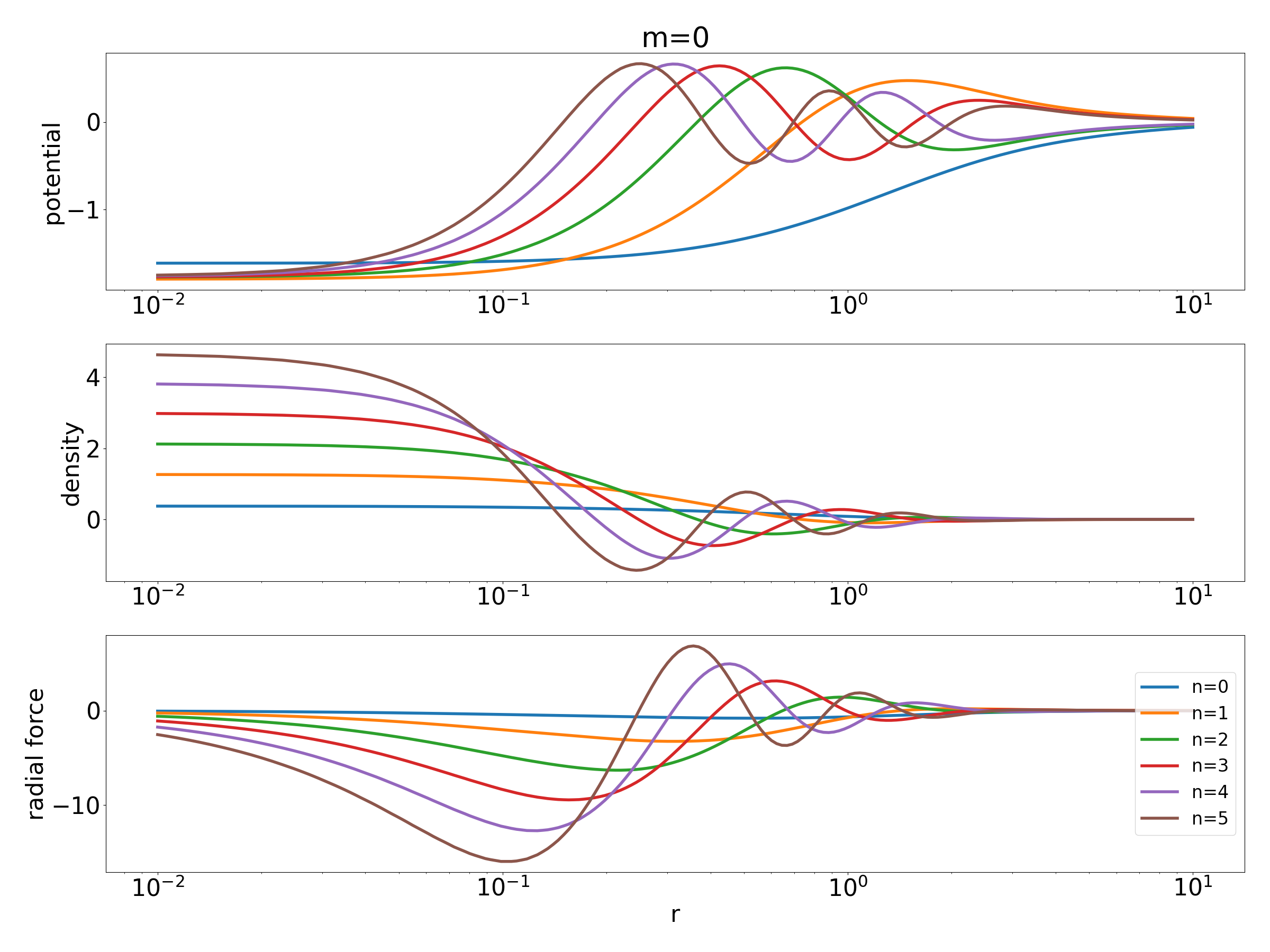
Figure 12: Biorthogonal $m=0$ basis functions for the two-dimensional exponential disk with scale length $a=1$. The color key describes the radial index, $n$. The $n=0$ basis function has no radial nodes. The $n=1$ function has one radial node. Each successive function has one more radial node. The exponential density conditioning leads to nodes distributed like the cumulative mass by construction.

A.3 Algorithm

Putting this development together, we may summarize the computation of the gravitational potential in $R,\phi,z$ as follows:

1. Choose the edge of the radial domain: $R$.

2. Choose a Bessel expansion order: $N$.

3. Choose $RK=\alpha_{m,N+1}$ to minimize the error matrix as described in Yu et al. (1998). This defines the value $K=\alpha_{m,N+1}/R$.

4. The evaluation knots are then as in equation (15) for $j\in[1,\ldots,N]$.

5. Compute the matrix $\mathbf{T}$ from equation (19).

6. Compute the vector $\mathbf{F}$ for the surface density $\Sigma_{m}$ to get the discrete Hankel transform: $\mathbf{G}=\mathbf{T}\cdot\mathbf{F}$.

7. Compute the potential integrand:

   $$\mathbf{K}=\left\{\frac{e^{-|\mathbf{k}|z}}{\mathbf{k}}\right\}\otimes\mathbf{G}$$

   or equivalently $K_{j}=-\exp(-k_{j}|z|)G_{j}/k_{j}$.

8. Compute the inverse discrete Hankel transform to get:

   $$\mathbf{\Phi}=\mathbf{T}\cdot\mathbf{K}$$

   .

9. Finally, the evaluation of $\Phi$ at an arbitrary value of $r$ may be accurately performed using equation (17) as an interpolation formula.

A.4 Discussion

The main advantages of the strategy outlined in this section for numerically evaluating the three-dimensional gravitational potential for a razor-thin disk are:

1. One can condition the biorthgonal Bessel-function basis on any well-behaved target density, similar to the three-dimensional case.

2. The Hankel transform necessary to obtain the off-plane potential is very accurate.

The disadvantages of this approach are:

1. It works well only for a basis with a finite extent. The Hankel transformation for an infinite domain is numerically challenging. We have had good success using QDHT, so we recommend the finite basis for this reason. This restriction to a finite-domain is not a problem in practice for simulations whose implementations are numerically finite.

2. The Bessel functions are asymptotically oscillatory and the truncation to order $N$ will leave their oscillatory imprint at larger radii. Again, this is not a problem for simulations where the larger disk radii are not dynamically important.

While the code implemented in exp allows the conditioning on the 2d Clutton-Brock basis, the computation of the vertical potential is less accurate for the same computational work using QDHT. This could be improved by truncating the basis and implementing Neumann boundary conditions with appropriate outgoing eigenfunctions. That has not been done here. Another solution might be an asymptotic numerical evaluation of the Hankel transform at large cylindrical radii patched onto a brute force quadrature at small radii. At this point, we recommend the Bessel basis for accuracy, especially for coupling the disk response another three-dimensional component such as a bulge or halo. If only the two-dimensional in-plane evaluations are needed (e.g. a two-dimensional disk in a fixed halo), both basis choices will be equally good.

Appendix B Hamiltonian perturbation theory

The bar growth and instability in a two-dimensional disk is mediated by the inner Lindblad resonance (ILR) as described in Lynden-Bell (1979). In essence, Lynden-Bell describes bar growth by determining the conditions for a test-particle orbit to precess towards the a quadrupole disturbance presented by the mean-field of all other orbits in the vicinity of the test particle (see Section 2.5 for more discussion).

To help understand the N-body dynamics described in Section 3, we use the same Hamiltonian perturbation theory to derive a constrained N-body simulation that excerpts the ILR interaction from the perturbation theory and treats it as the fundamental interaction between phase-averaged particles. The new simulation method is itself non-linear while reproducing the linear perturbation theory in the linear limit. The numerical method parallels the N-body method described in Section 2.2: it represents the mean gravitational field of the particle ensemble interacting near the ILR using a biorthogonal expansion. This development generalizes the well-known Hamiltonian Mean Field or cosine model (Chavanis et al., 2005) in philosophy, if not physical detail. The cosine model assumes that the potential of each pairwise interaction of particles $i,j$ on a ring with position angle $\theta$ is $\cos(\theta_{i}-\theta_{j})$. The model below is a cosine model whose coefficients depend on actions that exactly represent the orbit-averaged contributions to the mean field. The pairwise interactions are replaced with the interaction of each particle with the mean contribution of all particles. For brevity and with apologies for a small abuse of terminology, we will call this the BarHMF model. We will see in Section B.4 that the BarHMF model captures many of the interesting linear and non-linear aspects of bar growth and instability seen the the full N-body simulations. This correspondence allows us to use this model to help explain the N-body simulations in Section 3.

B.1 Perturbation theory

The linear response theory has been described in many places and this development parallels Tremaine and Weinberg (1984) and Weinberg (1991). Our goal here is to present enough of the mathematical derivation to motivate the hybrid N-body solution. We consider a non-axisymmetric gravitational potential:

$$U_{p}(\mathbf{r},t)=\sum_{m}U_{m}(r)e^{im(\phi-\Omega_{pm}t)}.$$ (28)

with a well-defined pattern speed, $\Omega_{pm}$, for each azimuthal harmonic, $m$. For comparison with the results in Section 3, we restrict ourselves to the single $m=2$ polar harmonic. We assume a regular axisymmetric background potential. The background potential is independent of the particle dynamics. The orbital dynamics may be fully expressed in action-angle coordinates. We will denote the angle and action vectors by $(\mathbf{w},\mathbf{I})$ where index 1 (2) is the radial (azimuthal) degree of freedom. To make explicit correspondence with the flat disk considered in this paper, we have $I_{1}=I_{r}$ (radial action) and $I_{2}=J=L_{z}$ (angular momentum) with $l_{1}=l_{r}$ and $l_{2}=l_{\phi}$. This allows us to expand any function of phase space as Fourier expansion:

$$U(\mathbf{w},\mathbf{I},t)=\sum_{m}\sum_{l_{1}^{\prime}=-\infty}^{\infty}\sum_{l_{2}^{\prime}=-m}^{m}W_{\mathbf{l}^{\prime}\,m}(\mathbf{I})e^{i(\mathbf{l}^{\prime}\cdot\mathbf{w}-m\Omega_{pm}t)},$$ (29)

where $\mathbf{l}=(l_{1},l_{2})$ and

$$W_{\mathbf{l}\,m}(\mathbf{I})=\frac{1}{(2\pi)^{2}}\oint dw_{1}dw_{2}e^{-i(\mathbf{l}\cdot\mathbf{w}-m\Omega_{pm}t)}U(\mathbf{w},\mathbf{I},t).$$ (30)

If we now specialize this to equation (28) with the assumption of a fixed axisymmetric background and $m=2$ only, we find

$$W_{\mathbf{l}\,2}(\mathbf{I})=\delta_{l_{2}\,2}\frac{1}{2\pi}\oint dw_{1}e^{[-i[l_{1}w_{1}+l_{2}f(w_{1})]}U_{2}(r(\mathbf{w},\mathbf{I}))$$ (31)

where $w_{2}=\phi+f(w_{1})$. The function $f(w_{1})$ represents the shift of azimuth from that of the guiding center owing to the radial motion (Tremaine and Weinberg, 1984). This is a direct consequence of conservation of angular momentum. Equation (31) is one-dimensional periodic quadrature that can be numerically computed to very high accuracy with little overhead.

The radial function $U_{2}(r)$ in equation (28) is arbitrary. Next, we will assume that $U_{2}(r)$ can be expanded in the biorthogonal basis as described in Appendix A: $\Phi_{mj}$ for $j\in[0,n_{max})$. This yields

$$U_{2}(r)=\sum_{j=0}^{n_{max}-1}a_{j}\Phi_{mj}(r)$$ (32)

where $a_{j}$ are expansion coefficients. We may explicitly compute and table the angle transforms for each $j$

$$W_{\mathbf{l}\,2}^{j}=\delta_{l_{2}\,2}\frac{1}{2\pi}\oint dw_{1}e^{[-i[l_{1}w_{1}+l_{2}f(w_{1})]}\Phi_{2\,j}(r(\mathbf{w},\mathbf{I}))$$ (33)

over a grid in $I_{1},I_{2}$ for numerical evaluation.

B.2 Averaging

We now apply the averaging principle. The idea is simple: near a particular resonance, the libration angle defined as $\mathbf{l}\cdot\mathbf{w}-\Omega_{p2}t$ is very slowly changing relative to either component of $\mathbf{w}$. This allows us to make a simple canonical transformation to a linear combination of angles and actions where one of the new coordinates is this libration angle by construction. Let the new angles and actions be ${\cal W}=(w_{s},w_{f})$ and ${\cal I}=(I_{s},I_{f})$, respectively. Let us choose the Type 2 generating function (Goldstein et al., 2002)

$$F_{2}(\mathbf{\cal I},\mathbf{w})=(\mathbf{l}\cdot\mathbf{w}-\Omega_{p2}t)I_{s}+w_{1}I_{f}.$$ (34)

Simple calculation immediately shows that $w_{s}=\mathbf{l}\cdot\mathbf{w}-\Omega_{p2}t$, $w_{f}=w_{1}$, $I_{1}=l_{1}I_{s}+I_{f}$ and $I_{2}=l_{2}I_{s}$. The new Hamiltonian is ${\cal H}=H-2\Omega_{p2}I_{s}$. There is some arbitrariness in the choice of $F_{2}$ but the important feature is that $w_{s}$ changes slowly compared to the change in $w_{f}$.

Armed with this development, we average equation (29) over a time interval $T$ chosen so that $2\pi/\Omega_{1}\ll T\ll 2\pi/(\mathbf{l}\cdot\mathbf{\Omega}-2\Omega_{p2})$. By construction, all terms in the sum are rapidly varying in this interval except for the one with $l_{1}^{\prime}=l_{1}$ and $l_{2}^{\prime}=l_{2}$. Our perturbed Hamiltonian for the averaged system reduces to a single term:

$$H_{1}(\mathbf{w},\mathbf{I})=W_{\mathbf{l}\,2}(\mathbf{I})e^{iw_{s}}.$$ (35)

Expressed in the biorthogonal basis, this may be written as

$$H_{1}(\mathbf{w},\mathbf{I})=\sum_{j=0}^{n_{max}-1}a_{j}W^{j}_{\mathbf{l}\,2}(\mathbf{I})e^{iw_{s}}.$$ (36)

Now, let us take some ensemble of $N$ particle trajectories. At any particular time $t$, a single trajectory indexed by $k$ contributes

$$\delta a_{j} = \int d\mathbf{r}\delta(\mathbf{r}-\mathbf{r}_{k}(t))\Phi_{mj}(r)e^{-im(\phi-\Omega_{p2}t)}$$ (37)

$$= \int dr\delta(r-r_{k}(t))\Phi_{mj}(r)\int d\phi\delta(\phi-\phi_{k}(t))e^{-im(\phi-\Omega_{p2}t)}$$

to the coefficient $a_{j}$ where $\delta(\cdot)$ is the Dirac delta function. The averaging principle requires an average of the fast action to get the slow contribution. The contribution of a single averaged trajectory indexed by $k$ to $a_{j}$ is

$$a^{k}_{j} = \frac{1}{2\pi}\oint dw_{f}\delta a_{j}$$ (38)

$$= \frac{\delta_{l_{2},m}}{2\pi}\oint dw_{f}\Phi_{l_{2}\,j}(r(\mathbf{w},\mathbf{I}))e^{-il_{2}(w_{2}-f(w_{1})-m\Omega_{p2}t)}$$

$$= e^{-i(l_{1}w_{1}+l_{2}w_{2}-m\Omega_{p2}t)}\frac{\delta_{l_{2},m}}{2\pi}\oint dw_{1}\Phi_{l_{2}\,j}(r(\mathbf{w},\mathbf{I}))e^{i(l_{1}w_{1}+l_{2}f(w_{1}))}$$

$$= e^{-iw_{s}}W_{\mathbf{l}\,2}^{j\ast}(\mathbf{I}),$$

where we used $w_{2}=\phi+f(w_{1})$ in the second equality, explicitly held $w_{s}$ fixed during the average of $w_{f}=w_{1}$ in the third equality, and identified $W_{\mathbf{l}\,2}^{j}(\mathbf{I})$ from equation (33). The values of $w_{s}$ and $\mathbf{I}$ are those of trajectory $k$.

The Hamilton equations for a particular phase trajectory then become:

$$\dot{w}_{s} =\quad\frac{\partial H}{\partial I_{s}}=\frac{\partial{\cal H}}{\partial I_{s}}+\frac{\partial H_{1}}{\partial I_{s}}= \mathbf{l}\cdot\mathbf{\Omega}-2\Omega_{p2}+e^{iw_{s}}\sum_{j=0}^{n_{max}-1}a_{j}\frac{\partial W^{j}_{\mathbf{l}\,2}(\mathbf{I})}{\partial I_{s}},$$ (39)

$$\dot{I}_{s} =-\frac{\partial H}{\partial w_{s}}= -ie^{iw_{s}}\sum_{j=0}^{n_{max}-1}a_{j}W^{j}_{\mathbf{l}\,2}(\mathbf{I}).$$ (40)

The first term in equation (39) is the unperturbed frequency of the slow motion. This frequency vanishes at the resonance. The final terms in each of equations (39) and (40) describe the perturbation from the quadrupole component contributed by each particle. This is a pendulum equation where the pendulum arm has a general dependence on the action of the particle.

B.3 The hybrid simulation method

We begin by adopting the biorthogonal basis from Appendix A that matches the simulations in Section 3. We represent the axisymmetric background potential by the spherical halo model from Section 2.1.1 for computational convenience and simplicity; using a combined disk, bulge, dark-matter halo background field is straightforward but not necessary for this demonstration. The particle motion remains planar by construction. Then, we tabulate the values of $W^{k}_{\mathbf{l}\,2}(\mathbf{I})$ on a two-dimensional grid in $\mathbf{I}$. The actions of the simulation particles can be chosen according to some distribution. For studies here, we distribute guiding centres in a smooth distribution in a particular annulus. The initial distribution of $w_{s}$ is chosen in one of two ways: (1) random in $[0,2\pi]$ or (2) uniformly spaced in $[0,2\pi)$ with an specific excess in a small interval of $(-\epsilon,\epsilon)$ to seed the perturbation. For Case 1, the small variations from uniform are sufficient to seed an instability for a bar-unstable system. For Case 2 without an excess, a uniformly distribution will remain close to equilibrium for an unreasonably long time. In other words, this choice relies on numerical noise to produce an asymmetry that grows. This motivates adding a small deviation to seed a disturbance.

Our simulation particles only contribute their quadrupole component from a single $\mathbf{l}$ term in equation (29) to the gravitational field. Each particle begins with a mass, actions $I_{f}$ and $I_{s}$ and slow angle $w_{s}$. Without external influences, the fast action $I_{f}$ is fixed throughout. However, under the influence of the Markov jump process described in Section 2.4, both $I_{f}$ and $I_{s}$ can change as described in Section 3.3.4. The fast action, $I_{f}$, changes result from the gravitational fluctuations and the slow action, $I_{s}$, changes as a result of the quadrupole field. Assume that we have $N$ particles of mass $m_{k}$ distributed as described in the previous paragraph. The mean-field potential is determined by summing the contributions of each particle to the $n_{max}$ numerically-determined coefficients $\hat{a}_{j}$:

$$\hat{a}_{j}=\sum_{k=1}^{N}m_{k}a^{k}_{j}=\sum_{k=1}^{N}m_{k}e^{-iw_{k}}W^{j\ast}_{\mathbf{l}\,2}(\mathbf{I}_{k}).$$ (41)

The averaging smooths out each particle’s spatial contribution from pericentre to apocentre. This results in a faster convergence with particle number $N$ and radial order $n_{max}$ than a traditional N-body code. If we define $J(E)$ as the maximum value of orbital angular momentum, $J$, at particular energy $E$, a converged series is obtained for $n_{max}=6$ for modestly eccentric orbits with $J/J(E)=0.8$.

The simulation proceeds by solving $2N$ first-order ODE defined by equations (39) and (40) for $w_{s}$ and $I_{s}$ respectively. Without any external perturbations, the fast actions $I_{f}$ are constant for the entire simulation. However, the background values for $\Omega_{1}(\mathbf{I})$, $\Omega_{2}(\mathbf{I})$, $W^{k}_{\mathbf{l}\,2}(\mathbf{I})$ and other phase-space quantities needed by equations (39) and (40) are naturally tabulated in $I_{1}$ and $I_{2}$ or $E$ and $L=I_{2}$. Thus, any changes in $I_{s}$ imply both changes $E$ and $L$. New values are computed using bilinear interpolation on precomputed grids of size $400\times 400$.

Unfortunately, this Hamiltonian flow is not explicitly separable which complicates the choice of an ODE solver. Recall that a Hamiltonian system is separable if the Hamiltonian can be written as $H(\mathbf{q},\mathbf{p})=K(\mathbf{p})+V(\mathbf{q})$ where $K$ and $V$ most often correspond to the kinetic and potential functions, and is non-separable otherwise. A separable system can be solved explicitly, using the well-known leapfrog algorithm or higher-order generalizations (Yoshida, 1990). This approach works because the Hamiltonian can be separated or split into two pieces that depend only on $\mathbf{q}$ or $\mathbf{p}$. For example, flows with $H(\mathbf{q},\mathbf{p})=K(\mathbf{p})$ and $H(\mathbf{q},\mathbf{p})=V(\mathbf{q})$ are both exactly solvable (see Sanz-Serna and Calvo 2018 for examples). To avoid an implicit method for the non-separable equations (39)–(40), we adopt the clever solution proposed by Tao (2016). Tao introduces an extended phase space with an extra copy of phase space $(\mathbf{x},\mathbf{y})$ that coincides with $(\mathbf{q},\mathbf{p})$ initially. The Hamiltonian of the extended system is the sum of three Hamiltonians:

$$\bar{H}(\mathbf{q},\mathbf{p},\mathbf{x},\mathbf{y})=H(\mathbf{q},\mathbf{y})+H(\mathbf{x},\mathbf{p})+\frac{\omega}{2}\left[(\mathbf{q}-\mathbf{x})^{2}+(\mathbf{p}-\mathbf{y})^{2}\right].$$ (42)

The first two terms are the original Hamiltonian function and the third term is a non-physical linear force that drives the two copies towards each other. One can solve each of the three Hamilonians with an explicit method. Recall that an explicit sympletic ODE solver is a Hamiltonian map. The combined mapping for the three separable Hamiltonians in equation (42) is the composition of three maps. The coupling parameter $\omega$ needs to be chosen large enough to keep the two phase-space copies, $(\mathbf{q},\mathbf{p})$ and $(\mathbf{x},\mathbf{y})$, close to each other but the solution is not sensitive to $\omega$ once so tuned. Tao estimates that the error for a solution of length $T$ is ${\cal O}(Th^{l}\omega)$ for a duration ${\cal O}(\min[h^{-l}\omega^{-1},\omega^{1/2}])$ where $l$ is the order using Yoshida (1990). Tao (2016) gives a detailed discussion of convergence and consistency. In practice, the Tao method produces high-accuracy solutions with little energy drift for the conservative time-independent system. However, unstable critical systems require large values of $\omega$ and some tuning effort especially for $N\mathrel{\hbox{\hbox to0.0pt{\hbox{\lower 4.0pt\hbox{$\sim$}}\hss}\hbox{$<$}}}400$. We compared our implementation of Tao’s algorithm to fourth-order Runga Kutta for verification. In practice, this method requires a much smaller time step than a traditional N-body code. The fourth-order ($l=4$) Tao method requires a comparable or larger number of function evaluations with similar long-term energy drift as fourth-order Runga Kutta at the same step size.

B.4 Test results

The simplest possible test of the new simulation method is the two-body quadrupole problem: two averaged particles that feel each other’s mutual potential along with the fixed monopole of the background system. This system is coupled pendulum and admits irregular motion. In the regular domain, the relative motion of the two interacting particles is oscillatory. Our first test solves equations (39) and (40) for $N=2$ and plots the the difference in $w_{s}$. The two particles have identical actions corresponding to a particles with $J/J_{max}(E)=0.8$ with guiding center radius of $r_{c}=3{\rm\,kpc}$; this corresponds to approximately one Milky-Way exponential scale length. The pericenter and apocenter of the unaveraged orbit is 0.006 and 0.012, respectively ($1.8$ and $3.6{\rm\,kpc}$ in Milky Way units, respectively). The initial position angles are displaced by 0.1 radians. The total mass of the two-particle system is $2\times 10^{-3}$ of the total background mass, $M=2\times 10^{9}{\rm\,M_{\odot}}$. These values are chosen to represent a typical ensemble of disk orbits in the vicinity of the disk scale length. None of these results depend qualitatively on this choice.

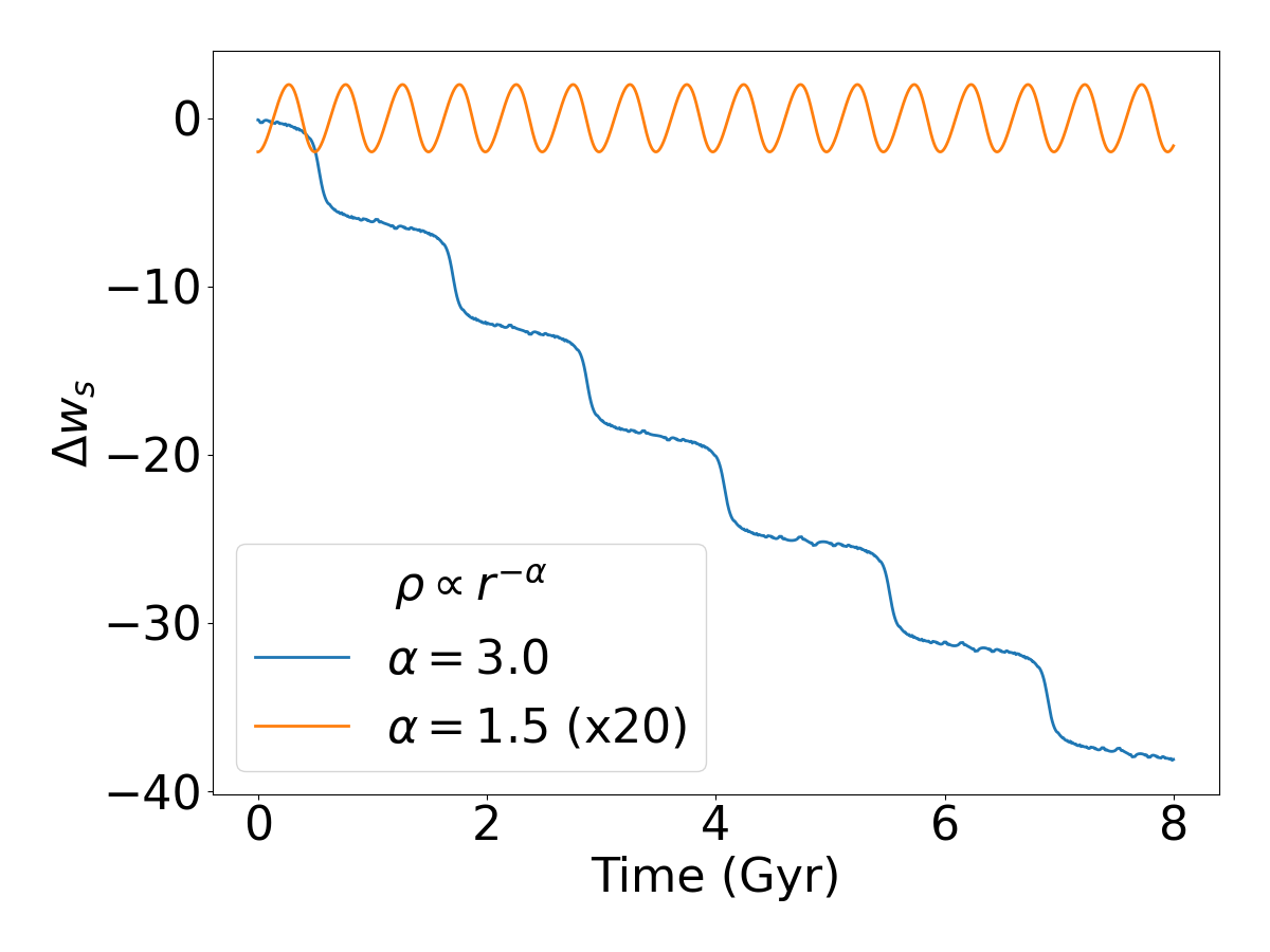
Figure 13: Difference in slow angle, $\Delta w_{s}$, for two particles with differently sloped rotation curves. The $\alpha=1.5$ model has a rising rotation curve with a positive Lydnen-Bell criterion value ${\cal L}$ and $\alpha=3.0$ has a falling rotation curve with a negative ${\cal L}$. The $\alpha=1.5$ curve is multiplied by factor of 20 to show the oscillations which would be too small to see otherwise.

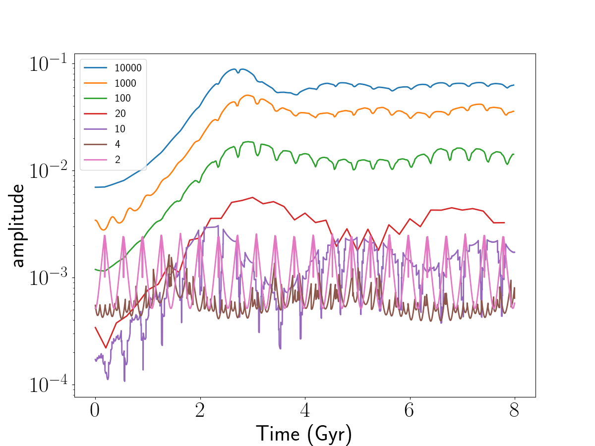
Figure 14: Bar amplitude as a function of particle number $N$ for the NFW-like background model with $\rho\propto r^{-1}$ in the vicinity of the particles. The amplitude is computed from a kernel density estimate of the distribution of $w_{s}$ for the $N$ particles.

We consider two different background models (eq. 2): one with $\alpha=1.5,\beta=0$ and one $\alpha=3.0,\beta=0$ with the default values of $r_{t}=1.5,r_{w}=0.2$ as described in Section 2.1.1. The Lynden-Bell criterion from equation (9) predicts that the first should bar promoting while the second should be bar avoiding. That is, the orbits will attract in the first case or librate and repel in the second case or rotate. Figure 14 presents the solutions of equations (39) and (40) and plots the the difference in $w_{s}$. This demonstrates the predicted behavior: the two particles librate for the $\alpha=1.5$ case which has ${\cal L}>0$ and rotate for the $\alpha=3.0$ case which has ${\cal L}<0$.

For $N\gg 1$, the particles can exchange slow action $I_{s}$ with the mean field and thereby with each other. We use the extremum excursion of the probability distribution for the $N$ values of $w_{s}$ in the interval $[0,2\pi)$ to estimate the amplitude of the resulting bar. The distribution is constructed using a kernel density estimator with the optimal Gaussian kernel width expression from Silverman (1986). To explore the change in bar amplitude with time for simulations of various $N$, we choose an the NFW-like background model (eq. 2 with $\alpha=1,\beta=2$). The model has $\rho\propto r^{-1}$ in the vicinity of the BarHMF particles and is explicitly bar promoting according to ${\cal L}$. The particle parameters are the same as the two-particle model with the same total particle mass, $M_{b}$: particles have identical actions corresponding to a particles with $J/J_{max}(E)=0.8$ and a single guiding center radius of $r_{c}=0.01$.

Figure 14 compares the bar amplitude from BarHMF runs with increasing values of $N$. The behavior for $N=2$ is sinusoidal libration as in Figure 14. For $N\mathrel{\hbox{\hbox to0.0pt{\hbox{\lower 4.0pt\hbox{$\sim$}}\hss}\hbox{$>$}}}10$, we begin to see a clear period of exponential growth followed by oscillation. As $N$ increases, the amplitude increases with otherwise similar behavior: the classic bar-like exponential growth phase followed by a steady state. The short-period modulution of $\approx 0.18$ is the one-particle libration time. This is corresponds to $\sim 300{\rm\,Myr}$ in Milky Way units. These modulations become weaker with increasing $N$ as expected. This figure also shows a longer period modulution in the steady-state phase that decreases in amplitude and possibly increases in period with increasing $N$. We speculate that this is the ongoing phase mixing of transient from the initial formation but have not yet investigated this in detail.

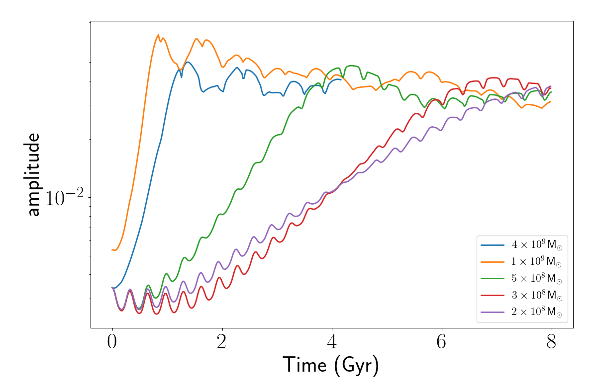
Figure 15: Bar amplitude variation as a function of disk mass, showing that the initial exponential growth is proportional to bar-particle mass. The model is the same as the one shown in Figure 14 and the total particle mass is shown in the legend.

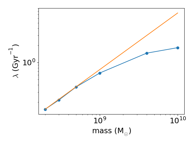
Figure 16: Exponential growth rate for the amplitude as a function of mass (blue) estimated from the curves in Fig. 16. The expected linear relation extrapolated from small mass is shown for comparison (orange). The expected linear scaling is only valid for small disk mass.

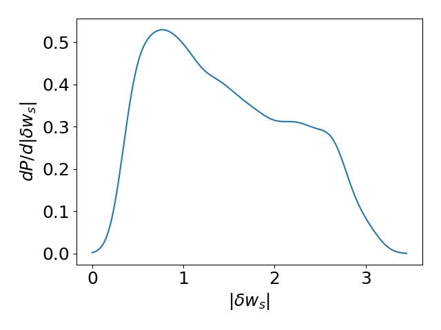
Figure 17: The distribution of the excursion angle, $|\delta w_{s}|$, in radians for the 9377 librating trajectories for the BarHMF run with $N=10000$ shown in Fig. 14. The excursion in apocentric position is $|\delta w_{s}|/2$. The apocentric distribution is approximately flat between $10^{\circ}$ and $70^{\circ}$ with a peak at $20^{\circ}$.

The exponential growth rate seen in Figure 14 is nearly the same for all $N\mathrel{\hbox{\hbox to0.0pt{\hbox{\lower 4.0pt\hbox{$\sim$}}\hss}\hbox{$>$}}}100$. Indeed, we expect the growth rate to depend on and increase linearly with total particle mass, $M_{b}$. Figure 16 demonstrates this with a sequence of simulations with $N=1000$ and varying mass with $M_{b}$ between $10^{8}{\rm\,M_{\odot}}$ and $10^{10}{\rm\,M_{\odot}}$. The growth rate is estimated as the slope of the rise in the log-linear plot, shown in Figure 16. This slope is linearly proportional $M_{b}$ until $M_{b}\approx 10^{9}{\rm\,M_{\odot}}$. For larger values, the slope increases more weakly with mass. For $M_{b}\mathrel{\hbox{\hbox to0.0pt{\hbox{\lower 4.0pt\hbox{$\sim$}}\hss}\hbox{$>$}}}4\times 10^{9}{\rm\,M_{\odot}}$ the increase in slope is weakly than linear, suggesting that bar is no longer following the linear predictions. Rather, it is growing as fast as it can limited by the intrinsic characteristic time of BarHMF model. The regime is typical of bar growth in unstable high-mass disks typical of N-body simulations of isolated galaxies.

For a final demonstration of the correspondence between the BarHMF and the full N-body simulations, we compare the fraction of trapped, librating orbits after bar formation is complete with the untrapped, rotating fraction. We do this by computing the difference between the position angle of each particle and the mean position angle of the entire ensemble as a function of time. The variation of the distribution around the ring is very close to sinusoidal. We use the same the probability distribution estimate of $w_{s}$ used to infer the amplitude to find the position angle of the peak, $\theta_{PA}$. This yields a time series of excursions for the angle of each quadrupole particle relative to the bar position angle: $\delta w_{s}(t)=w_{s}(t)-\theta_{PA}(t)$. Then, we estimate the width of $\delta w_{s}$ for each trajectory by computing the distance between the extremal values for all $t$, denoted as $|\delta w_{s}|$. A librating (rotating) trajectory has $|\delta w_{s}|$ smaller (larger) than $\pi$. Using this to classify BarHMF trajectories, we find that 94% of the distribution is in libration by the end of the simulation at $T=4{\rm\,Gyr}$. Figure 17 shows the distribution of widths $|\delta w_{s}|$ for the ensemble of librating trajectories. This distributions peaks at $0.7\,\mbox{rad}$ (or $40^{\circ}$) with a long heavy tail to large libration angle. This implies an excursion about the bar position at apocenter of $|\delta w_{s}|/2$ or $0.35\,\mbox{rad}$ (or $20^{\circ}$). Petersen et al. (2021) find a similarly large trapped fraction of $x_{1}$ orbits of approximately 80% in the bar vicinity. Moreover, the trapped BarHMF shows a broad tail of libration amplitudes which is also similar to the distributions seen in N-body simulations. A precise correspondence to the N-body simulations from Section 3 should not be expected for two reasons: (1) we have not included the background potential of the disk itself; and (2) we have not fully distributed the BarHMF particles according to the disk phase-space distribution function. Such simulations are possible but would require an intensive computational campaign that is beyond the scope of this preliminary study. Nonetheless, the good correspondence between the major features of bar growth and saturation suggest that the simple perturbation theory captures much of the bar instability mechanism and supplies a good model for further applications (Sec. B.5).

B.5 Topics for future work

This paper focuses on the classic $m=2,l_{1}=-1,l_{2}=2$ bar instability. Only one term in equations (28) and (29) is required. However, the BarHMF simulation can be trivially generalized to include multiple resonances $(m,l_{1},l_{2})$, The extended model can be used, for example, to explore non-linear resonance coupling in barred system in the non-linear regime. Technically, this requires adding multiple commensurabilities of the form in equation (29) and eliminating averaging in favor of the full equations of motion for $(\mathbf{w},\mathbf{I})$. For example, consider adding the classic 4:1 bar resonance (Contopoulos, 1988). The pattern speed is the same for each harmonic: $\Omega_{p}\equiv\Omega_{p2}=\Omega_{p4}$. The commensurability is $\Omega_{r}=4(\Omega_{\phi}-\Omega_{p})$ and gives an new term with $m=4,l_{1}=-1,l_{2}=4$. Each BarHMF particle now interacts with two shapes depending on its action values $(I_{r},I_{\phi})$: a dumbbell shaped quadrupole density and a 4-lobed octopole density (e.g. two pyramids joined at their bases or two orthogonally-oriented dumbbells). Each additional resonant term adds a new degree of freedom corresponding to the slow angle action from equation (34). In addition, combinations with multiple $m$ orders will have separate sets of coefficients for each order from equation (41).

With one term, the BarHMF simulation is an ensemble of interacting pendula. This system is intrinsically irregular. Indeed some of the simulations described in Appendix B.4 show evidence of chaotic behavior. As we add more terms, we introduce the possibility additional chaotic channels such as resonance overlap (Chirikov, 1979) and weak chaotic transport (Manos and Athanassoula, 2011). The BarHMF model is ideal model for investigating the details of multiple resonance phenomena in barred systems. This ability to study the interactions of specific resonances is ideal for isolating and determining their relevance to barred systems in traditional simulations and Nature. With only several specific resonant terms, the computational effort will remain modest.

The examples in Appendix B.4 assume a spherical background potential for expediency and the same two-dimensional basis described in Appendix A and used for the simulations Section 3. We may couple the in-plane dynamics of the BarHMF model to other galactic components using the potential theory described in Appendix A. For example, we can study the evolution of the bar in the presence of dynamical friction and investigate the dependence on the dark-matter halo properties. The BarHMF model presents a new opportunity to understand the changes and redistribution of the bar orbits under torque, a subject which remains poorly understood dynamically. This exploration might be especially productive with BarHMF which provides the opportunity to explicitly identify interactions between multiple resonances.