Does AI help humans make better decisions?
A methodological framework for experimental evaluation

Abstract

The use of Artificial Intelligence (AI) based on data-driven algorithms has become ubiquitous in today’s society. Yet, in many cases and especially when stakes are high, humans still make final decisions. The critical question, therefore, is whether AI helps humans make better decisions as compared to a human alone or AI alone. We introduce a new methodological framework that can be used to answer experimentally this question with no additional assumptions. We measure a decision maker’s ability to make correct decisions using standard classification metrics based on the baseline potential outcome. We consider a single-blinded experimental design, in which the provision of AI-generated recommendations is randomized across cases with a human making final decisions. Under this experimental design, we show how to compare the performance of three alternative decision-making systems — human-alone, human-with-AI, and AI-alone. We apply the proposed methodology to the data from our own randomized controlled trial of a pretrial risk assessment instrument. We find that AI recommendations do not improve the classification accuracy of a judge’s decision to impose cash bail. Our analysis also shows that AI-alone decisions generally perform worse than human decisions with or without AI assistance. Finally, AI recommendations tend to impose cash bail on non-white arrestees more often than necessary when compared to white arrestees.

Keywords: algorithmic decision-making, criminal justice, fairness, experimental design, misclassification

1 Introduction

Artificial Intelligence (AI), or more broadly data-driven algorithms, have found a wide range of applications in today’s society, including judicial decisions in the criminal justice system, diagnosis and treatment decisions in medicine, and recommendations in online advertisement and shopping. And yet, in many settings and especially when stakes are high, humans still make final decisions. The critical question, therefore, is whether AI recommendations help humans make better decisions as compared to a human alone or AI alone (Imai et al., 2023a).

Recent literature has largely focused on questions of whether or not AI recommendations are accurate or biased (e.g., Barocas et al., 2017; Corbett-Davies and Goel, 2018; Chouldechova and Roth, 2020; Mitchell et al., 2021; Imai and Jiang, 2023). However, AI recommendations may not improve the accuracy of human decisions if, for example, the human decision-maker selectively ignores AI recommendations (e.g., Hoffman et al., 2018; Lai et al., 2021; Cheng and Chouldechova, 2022). Similarly, the fairness of such an AI-assisted human decision-making system depends on how the bias of AI system interacts with that of human decisions.

In this paper, we introduce a new methodological framework for researchers to evaluate experimentally whether the provision of AI recommendations helps humans make better decisions. We formulate the notion of a decision-maker’s ‘ability’ as a classification problem by combining a standard confusion matrix with the potential outcomes framework of causal inference (Neyman, 1923; Rubin, 1974). For example, when deciding whether to impose cash bail on an arrestee or to release them on their “own recognizance” (i.e., an arrestee can be released without depositing money with the court; known in our application as ‘signature bond’), a judge must balance public safety and efficient court administration against various costs of incarceration. Thus, the judge’s decision-making ability can be defined as the degree to which they can correctly classify the as-yet unobserved arrestee’s behavior upon release. Under the proposed framework, we introduce a variety of classification ability measures. If AI recommendations are helpful, their provision should improve a human decision-maker’s ability to correctly classify potential outcomes.

This reasoning demonstrates that a primary methodological challenge in evaluating the the impact of various decision-making systems is the so-called selective labels problem; the decision-makers themselves determine, by making non-random decisions, which potential outcomes are observed (e.g., Lakkaraju et al., 2017). In the aforementioned example, since judges decide which arrestees are released on their own recognizance or subject to cash bail, we would not observe whether an arrestee who received the cash bail decision would have committed a new crime if a judge were to release them without additional conditions.

To overcome this problem, we consider an experimental design, in which the provision of AI recommendations is randomly assigned to human decision-makers across cases. Such an experimental design is feasible even in settings where, for policy or other reasons, a human, rather than an AI system, makes final decisions. We consider a single-blinded treatment assignment, which guarantees that the provision of AI recommendations affects the outcome only through human decisions.

Under this experimental design, we show that, with no additional assumption, it is possible to point-identify the difference in misclassification rates, or more generally the difference in classification risk, between the human-alone and human-with-AI systems even though the risk of each decision-making system is not identifiable. In addition, although the proposed experimental design does not include the use of an AI-alone decision-making system as one of the treatment conditions, we derive bounds on the classification ability differences between an AI-alone system and a human-alone or human+AI system. We show empirically that these bounds can be informative, making it possible for researchers to evaluate and compare the performance of these decision-making systems without imposing additional assumptions.

1.1 Experimental evaluation of a public risk assessment instrument

We apply our methodology to our own randomized controlled trial (RCT) to assess how an AI-generated predisposition risk assessment instrument, called the Public Safety Assessment (PSA), affects judges’ decisions at a criminal first appearance hearing, or “bail hearing” (Greiner et al., 2020; Imai et al., 2023a). In Dane County, Wisconsin, where we conducted the RCT, a judge at a first appearance hearing must decide whether to release an arrestee on their own recognizance or to impose cash bail as a condition of release. In this county, own recognizance release is called a “signature bond,” the term we will use in the remainder of this paper.

As mentioned earlier, if a judge assigns an arrestee a signature bond, the arrestee need not deposit money with the court to achieve pretrial release. For cash bail, the arrested individual must deposit the specified amount with the court to be released (note that there is no bail bondsman industry in Wisconsin). The decision between signature bond and cash bail does not conclusively determine whether an arrestee will achieve pretrial release. For example, some arrestees assigned cash bail in fact pay it and thus obtain their pretrial freedom, while others assigned signature bonds remain incarcerated because immigration or other criminal justice authorities request a ‘hold’ from the relevant jail. Additionally, in Dane County, the judge at the first appearance hearing can impose other conditions of release, such as monitoring, drug testing, or stay-away orders. For the purposes of this paper, however, we ignore these other decisions.

The PSA provides information to the judge for each decision regarding the arrested individual’s risk of (1) failure to appear (FTA) at subsequent court dates, (2) new criminal activity (NCA), and (3) new violent criminal activity (NVCA). In the RCT, the judge receives the PSA for a randomly selected subset of all first appearance/bail hearings (see Greiner et al., 2020, for details of the PSA instrument and experiment).

The PSA provides three numerical scores that correspond to its classification of FTA, NCA, and NVCA risks. The FTA and NCA risk scores have a total of six levels, while the NVCA risk score is binary. Nine factors about prior criminal history as well as age, the only demographic factor, serve as inputs to construct the PSA’s scores; neither race nor gender is an input. Finally, a deterministic formula called the Decision-Making Framework (DMF) combines the PSA’s three risk scores with other information, such as a jurisdiction’s resources and risk misbehavior tolerance, to produce an overall recommendation of either cash bail or signature bond. This overall PSA-DMF recommendation is the focus of our analysis in this paper.

To demonstrate our methodology, we analyze the interim data from this experiment, which are based on a single year of follow-up from the first 12 (of 30) months of randomization. We will use a slightly updated version of the preliminary data from this experiment, which was originally analyzed by Imai et al. (2023a) and has been subsequently made publicly available as Imai et al. (2023b).

		AI
		Signature	Cash
		bond	bail
	Signature	$54.1\%$	$20.7\%$
	bond	$(510)$	$(195)$
Human	Cash	$9.4\%$	$15.8\%$
	bail	$(89)$	$(149)$

		AI
		Signature	Cash
		bond	bail
	Signature	$57.3\%$	$17.1\%$
	bond	$(543)$	$(162)$
Human+AI	Cash	$7.4\%$	$18.2\%$
	bail	$(70)$	$(173)$

Table 1: Comparison between human decisions and AI-generated recommendations. The left table compares the AI recommendations (columns) against the judge’s decisions without AI recommendations (rows). Similarly, the right table compares the AI recommendations (columns) with the decisions made by a human judge who was provided with AI recommendations (rows). Each cell presents the proportion of corresponding cases with the number of such cases in parentheses.

Table 1 compares the judge’s decisions with the AI-generated recommendations (left table) and with the human-with-AI decisions (right). The number in each cell represents the proportion of corresponding cases with the number of such cases in parentheses. We find that human decisions, with or without AI recommendations, do not always agree with the AI recommendations. Indeed, the judge goes against the AI recommendations for slightly more than 30% of the cases. In the cases of disagreement, the AI recommendations tend to be harsher than human decisions. When provided with the AI recommendations, the judge disagrees with them slightly less often (by approximately five percentage points). However, even in these cases, there exists a substantial amount of disagreement between the human decisions and AI recommendations. Similar to the human-alone vs. AI-alone comparison, when they disagree, the AI recommendations tend to harsher than the human-with-AI decisions.

A primary goal of our empirical analysis is to evaluate whether AI recommendations improve judges’ classification ability in decision-making. In addition, we are also interested in comparing the classification ability of the AI-alone decisions with that of human decision. As mentioned above, the key challenge is the presence of selective labels: for cases where the judge issued a cash bail decision we do not observe the counterfactual outcome (FTA, NCA, NVCA) under a signature bond decision. The evaluation of the AI-alone decision-making system in itself is even more difficult because the experiment does not have an AI-alone condition. Our proposed methodological framework shows how to overcome these challenges with no additional assumptions beyond those guaranteed by the experimental design.

The results of our empirical analysis presented in Section 3 show that AI-generated recommendations do not significantly improve the classification ability of judge’s decision-making. For example, the misclassification rate of judge’s decisions is unchanged when the AI recommendations are provided. We also find that AI-alone decisions tend to perform worse than either human-alone or human-with-AI decisions. For both FTA and NVCA, the misclassification rate of AI-alone decisions is significantly greater than human decisions with or without AI recommendations. In particular, the AI system tends to have a greater proportion of false positives (i.e., imposing cash bail on an arrestee who would not commit a crime if released on their own recognizance). Finally, we show that the AI system tends to yield more false positives for non-white arrestees when compared to white arrestees, but such racial disparity is not found for human decisions.

1.2 Related literature

Existing literature on algorithmic decision-making has primarily focused on three areas: (i) the performance evaluation of algorithms in terms of their underlying classification tasks (e.g., Berk et al., 2016; Goel et al., 2016; Kleinberg et al., 2018; Rambachan et al., 2022), (ii) issues of algorithmic fairness and the potential for biased algorithmic or human recommendations (e.g., Barocas et al., 2017; Corbett-Davies and Goel, 2018; Chouldechova and Roth, 2020; Mitchell et al., 2021; Arnold et al., 2021, 2022; Imai and Jiang, 2023), and (iii) understanding how humans incorporate algorithmic recommendations into their decision-making (e.g., Binns et al., 2018; Cai et al., 2019; Lai et al., 2021; Cheng and Chouldechova, 2022; Imai et al., 2023a).

We focus on the following question that sits at the intersection of these three areas; Do AI recommendations help humans make better decisions than those made by human alone or AI alone? Other scholars have proposed using a classification framework with selective labels to consider the performance of algorithmic decision-making (e.g., Goel et al., 2016; Kleinberg et al., 2018; Rambachan et al., 2022). In contrast, we focus on the relative gains of AI recommendations over human decisions and use an RCT to identify more credibly our key quantities of interest with no additional assumptions.

Methodologically, our work contributes to a growing literature that addresses the selective labels problem when evaluating human decisions and AI recommendations. In particular, we consider an experimental design that randomizes the provision of AI recommendations while single-blinding the treatment assignment so that AI recommendations affect the outcome only through human decisions. We show that under this experimental design, it is possible to evaluate precisely the classification performance of human-alone, AI-alone, and human-with-AI decision-making systems. In contrast, related studies have largely been restricted to observational studies. For example, previous works exploit discontinuities at algorithmic thresholds and staggered roll-outs of algorithms, assuming that decisions are unconfounded (e.g. Berk, 2017; Albright, 2019; Stevenson and Doleac, 2022; Coston et al., 2021; Guerdan et al., 2023), or use survey evaluations (e.g., Miller and Maloney, 2013; Skeem et al., 2020).

Several studies have advocated designs that use quasi-random assignment to decision-makers with different decision rates. They use the differing decision rates as an instrumental variable to estimate various performance measures of AI recommendations relative to human decision-makers (e.g. Kleinberg et al., 2018; Dobbie et al., 2018; Arnold et al., 2022; Angelova et al., 2023). Unlike these studies, we consider an experimental setting where we are able to guarantee the required identification assumptions by design. Furthermore, while related approaches have been used to evaluate algorithmic decisions, we also evaluate the performance of human decision-makers with and without AI recommendations as well as the performance differences among them. Closest to our approach is Angelova et al. (2023), who compare AI-assisted human decisions to those of the algorithm by studying cases, in which humans override the algorithmic recommendation (see also Hoffman et al., 2018). Our framework is also similar to the one proposed by Imai et al. (2023a), but we focus on a single potential outcome rather than joint potential outcomes, allowing us to avoid making additional assumptions.

In this paper, we take a partial identification approach that bounds the quantities of interest when point identification is not possible (e.g., Manski, 2007). This methodological development is related to partial identification approaches proposed by Rambachan (2021) and Rambachan et al. (2022). In particular, Rambachan et al. (2022) consider general approaches to partial identification of the predictive performance of classification algorithms. In contrast, we focus on comparing the predictive performance of the aforementioned three different decision-making systems that involve humans and/or AI, leading to different identification results.

2 The Proposed Methodological Framework

In this section, we introduce a methodological framework that can be used to evaluate experimentally the relative performance of human-alone, AI-alone, and human-with-AI decision-making systems. Our framework proposes an experimental design, formalizes a decision-maker’s ability as a classification problem, and establishes identification results regarding various quantities and comparisons of interest. We now discuss each of these components in turn.

2.1 Experimental design

We consider an RCT, in which the provision of an AI recommendation is randomized across cases with a human making final decisions. Let $A_{i}\in\{0,1\}$ represent the binary AI-generated recommendation for case $i$. We assume that AI recommendations can be computed for all cases. In our application, $A_{i}=1$ means that AI recommends cash bail while $A_{i}=0$ indicates that AI recommends a signature bond. We use $Z_{i}\in\{0,1\}$ to denote the binary treatment variable representing the provision of such an AI recommendation. In our experiment, $Z_{i}=1$ indicates that case $i$ is assigned to a human judge with an AI recommendation, whereas $Z_{i}=0$ means that no AI recommendation is given to the judge.

This experimental design is applicable even when stakes are high and a human must make final decisions. The proposed methodology can be generalized to settings with more than two treatment conditions. For example, experimenters may use different AI systems or include an AI-alone decision as a separate treatment arm. For the sake of simplicity, we focus on the binary case of two treatment arms in this paper.

We use $D_{i}\in\{0,1\}$ to denote the observed binary decision made by a human. In our application, $D_{i}=1$ represents a judge’s decision to require cash bail as opposed to signature bond. In a medical setting, $D_{i}=1$ may signify a doctor’s decision to prescribe medication rather than not to treat. Since the decision can be affected by the AI recommendation, we use potential outcomes notation and denote the decision under the treatment condition $Z_{i}=z$ as $D_{i}(z)$. That is, $D_{i}(1)$ and $D_{i}(0)$ represent the decisions made with and without an AI recommendation, respectively. The observed decision, therefore, is given by $D_{i}=D_{i}(Z_{i})$.

In addition, let $Y_{i}\in\{0,1\}$ denote the binary outcome of interest. Without loss of generality, we assume that $Y_{i}=1$ represents an undesired outcome relative to $Y_{i}=0$. In our empirical application, this variable represents whether or not an arrestee fails to appear in court (FTA), or engages in new criminal activity (NCA) or new violent criminal activity (NVCA).

We consider the use of single-blinded treatment assignment. In our application, this means that an arrestee does not know whether a judge receives an AI recommendation. In other words, we assume that the provision of an AI recommendation, or lack thereof, can affect the outcome only through the human decision. Formally, let $Y_{i}(z,d)$ denote the potential outcome under the treatment condition $Z_{i}=z$ and the decision $D_{i}=d$. The single-blinded experiment assumption implies $Y_{i}(0,d)=Y_{i}(1,d)=Y_{i}(d)$ for any $d,z$ where the observed outcome is given by $Y_{i}=Y_{i}(D_{i}(Z_{i}))$.

In sum, our proposed experimental design requires two assumptions: randomization and single-blindedness of treatment assignment. We formally present these two assumptions here.

Assumption 1 (Single-blinded random treatment assignment)

The treatment assignment $Z_{i}$, potential decisions $D_{i}(z)$, and potential outcomes $Y_{i}(z,D_{i}(z))$ satisfy:

1. Single-blinded treatment: $Y_{i}(z,D_{i}(z))=Y_{i}(z^{\prime},D_{i}(z^{\prime}))$ for all $z,z^{\prime}$ such that $D_{i}(z)=D_{i}(z^{\prime})$.

2. Randomized treatment: $Z_{i}\ \raisebox{0.50003pt}{\rotatebox[origin={c}]{90.0}{$\models$}}\ \{A_{i},\{D_{i}(z),Y_{i}(d)\}_{z,d\in\{0,1\}}\}$

Our notation implicitly assumes no spillover effects across cases. In our application, this means that a judge’s decision should not be influenced by the treatment assignments of prior cases. Finally, we assume that we have an independently identically distributed sample of cases with size $n$ from a target distribution $\mathcal{P}$, i.e., $(D_{i}(0),D_{i}(1),Y_{i}(0),Y_{i}(1))\overset{i.i.d.}{\sim}\mathcal{P}$. In subsequent sections, we will omit the $i$ subscript from expressions whenever convenient.

The above randomization assumption can be extended to covariate-dependent random assignment designs based on pre-treatment covariates such as blocking and matched-pair designs. Conditional on these covariates, we can derive the identification results that are equivalent to those presented in the following sections. To avoid notational burden, we focus on the case of randomized treatment assignment without covariates.

2.2 Measures of classification ability

We use a classification framework to formalize the ‘classification ability’ of a decision-maker that we use to evaluate each decision-making system. We focus on the baseline potential outcome $Y(0)$. In our application, this corresponds to the outcome we would observe (e.g., NCA) if an arrestee is released on their own recognizance ($D=0$).

		Decision
		Negative $(D=0$)	Positive $(D=1$)
	Negative ($Y(0)=0$)	True Negative (TN)	False Positive (FP)
		$\ell_{00}$	$\ell_{01}$
Outcome	Positive ($Y(0)=1$)	False Negative (FN)	True Positive (TP)
		$\ell_{10}=1$	$\ell_{11}$

Table 2: Confusion matrix for each combination of baseline potential outcome $Y(0)$ and decision $D$. Each cell is assigned a loss $\ell_{yd}$ for $y,d\in\{0,1\}$. The loss is standardized by setting $\ell_{10}=1$.

Table 2 shows the confusion matrix for all four possible pairs of baseline potential outcome $Y(0)$ and decision $D$. If the baseline potential outcome is negative in the classification sense, i.e., $Y(0)=0$ (e.g., an arrestee would not commit a new crime) and the decision is also negative, i.e., $D=0$ (e.g., a judge decides to assign signature bond), then we call this instance a ‘true negative’ or TN. In contrast, if the baseline outcome is positive (i.e., an undesired outcome in our application) and yet the decision is negative (e.g., a judge decides to release the arrestee on their own recognizance), then this instance is called ‘false negative’ or FN. False positives (FP) and true positives (TP) are similarly defined.

Using this confusion matrix, we can derive a range of classification ability measures. To do so, we first assign a loss (or negative utility) to each cell of the confusion matrix and then aggregate across cases. As shown in Table 2, let $\ell_{yd}$ denote a loss that is incurred when the baseline potential outcome is $Y(0)=y$ and the decision is $D=d$ for $y,d\in\{0,1\}$. Without loss of generality (no pun intended), we set the loss of a false negative to one, i.e., $\ell_{10}=1$.

This setup allows for both symmetric and asymmetric loss functions (Ben-Michael et al., 2023). If a false positive (e.g., unnecessary cash bail) and a false negative (e.g., signature bond, resulting in FTA/NCA/NVCA) incur the same loss, i.e., $\ell_{01}=1$, then the loss function is said to be symmetric. An asymmetric loss function arises, for example, if avoiding false negatives is deemed more valuable than preventing false positives, i.e., $\ell_{01}<1$. To simplify the exposition, we will consider loss functions where true negatives and true positives incur zero loss (i.e., $\ell_{11}=\ell_{00}=0$; see Appendix S1 for a discussion of generic loss functions).

Once the loss function is determined, we can define the classification risk (or expected classification loss) as the average of the the false negative proportion (FNP) and false positive proportion (FPP), weighted by their respective losses,

$$R(\ell_{01})\ =\ q_{10}+\ell_{01}q_{01},$$ (1)

where $q_{yd}=\Pr(Y(0)=y,D=d)$ for $y,d\in\{0,1\}$, and thus, $q_{10}$ and $q_{01}$ represent FNP and FPP, respectively.

Under this framework, we can also define a variety of ability measures. Examples include: (1) misclassification rate $=q_{10}+q_{01}=R(1)$, which represents the overall proportion of incorrect decisions, (2) false discovery rate $=q_{01}/(q_{01}+q_{11})$, which is equal to the proportion of incorrect decisions among positive decisions, (3) false negative rate $=q_{10}/(q_{10}+q_{11})$, which is the proportion of incorrect decisions among positive baseline outcomes, and (4) false positive rate $=q_{01}/(q_{00}+q_{01})$, which equals the proportion of incorrect decisions among negative baseline outcomes. See Appendix S3 for more details.

We use these measures of classification ability to evaluate three decision-making systems: human-alone, human-with-AI, and AI-alone. We are particularly interested in contrasting the classification abilities of these three systems. For example, the comparison of human-alone and human-with-AI tells us whether AI recommendations are able to improve human decision-making.

These classification ability measures can also be used to measure one possible aspect of the fairness of decision-making systems. In particular, one could estimate an ability measure for a subpopulation defined by a protected attribute (e.g., race and gender) and examine whether classification ability varies across these different groups. We may expect a fair decision-making system to make similar decisions across cases with the same value of potential outcome.

Prior work has considered these classification ability measures. For example, in the pre-trial risk assessment setting, Angelova et al. (2023) consider the misconduct rate among released defendants; this corresponds to the false negative rate. Dobbie et al. (2018) consider the proportion of individuals who are detained erroneously, i.e., the false discovery rate. Other work develop a more general framework. For instance, Rambachan et al. (2022) consider a generalized notion of performance that includes functions of the confusion matrix as well as other measures like calibration and mean square error, which we do not consider here.

One important limitation of our framework and related approaches, however, is that we only consider the baseline potential outcome rather than the joint potential outcomes. The “correct” or “wrong” decision might be depend on both potential outcomes instead of the baseline potential outcome alone. Unfortunately, the consideration of joint potential outcomes requires much stronger assumptions than those considered under our approach.

Nevertheless, Imai et al. (2023a) introduce a principal stratification framework that considers the joint set of potential outcomes and three principal strata of individuals: (1) preventable cases $(Y(1),Y(0))=(0,1)$) — individuals who would engage in misconduct only if released, (2) risky cases $(Y(1),Y(0))=(1,1)$) — individuals who would engage in misconduct regardless of the judge’s decision, and (3) safe cases $(Y(1),Y(0)=(0,0)$) — individuals who would not engage in misconduct regardless of the detention decision. The authors focus on the effect of provision of the AI recommendation on the human decision, conditioned on these principal strata. Imai and Jiang (2023) also introduce a related fairness notion, called principal fairness. In Appendix S2, we show that these principal causal effects are equivalent to particular functions of the confusion matrix under the special case of strong monotonicity, in which individuals with cash bail decisions never engage in misconduct (i.e. $Y(1)=0$).

2.3 Comparing human decisions with and without AI recommendations

We first demonstrate how to compare human decisions with versus without AI recommendations. As noted earlier, a primary methodological challenge is the selective labels problem. Specifically, we observe the baseline potential outcome under the negative decision $Y(0)$ only for some cases where the decision is actually negative, i.e., $D=0$. Despite this problem, we show that under the experimental design introduced in Section 2.1, it is possible to point-identify the difference in misclassification rate or more generally the difference in classification risk between human decisions with and without AI recommendations.

Formally, define $p_{yda}(z)$ as the probability that the outcome is equal to $y$, the decision under treatment assignment $z$ is equal to $d$, and the AI recommendation is equal to $a$:

$$p_{yda}(z)\ :=\ \Pr(Y(0)=y,D(z)=d,A=a)$$

for any $y,d,a,z\in\{0,1\}$. With this notation, we can write the confusion matrix for human decisions under treatment assignment $z$ as follows:

$$C_{\textsc{Human}}(z)=\left[\begin{array}[]{c c}p_{000}(z)+p_{001}(z)&\color[rgb]{0,0,1}{p_{010}(z)}+\color[rgb]{0,0,1}{p_{011}(z)}\\ p_{100}(z)+p_{101}(z)&{{\color[rgb]{0,0,1}p_{110}(z)}}+{{\color[rgb]{0,0,1}p_{111}(z)}}\end{array}\right]=\left[\begin{array}[]{c c}p_{00\cdot}(z)&{{\color[rgb]{0,0,1}p_{01\cdot}(z)}}\\ p_{10\cdot}(z)&{{\color[rgb]{0,0,1}p_{11\cdot}(z)}}\end{array}\right],$$ (2)

where $C_{\textsc{Human}}(0)$ and $C_{\textsc{Human}}(1)$ correspond to the confusion matrix for the human-alone and human-with-AI decision-making systems, respectively. For ease of notation, when marginalizing over the outcome, decision, or AI recommendation, we will use a dot in lieu of the corresponding subscript, i.e., $p_{y0\cdot}(z):=\Pr(Y(0)=y,D(z)=0)$ for $y,z\in\{0,1\}$.

Under the assumption of single-blinded randomized treatment assignment (Assumption 1), we can identify the terms in black as $p_{y0a}(z)=\Pr(Y=y,D=0,A=a\mid Z=z)$ and $p_{y0\cdot}(z)=\Pr(Y=y,D=0\mid Z=z)$. Thus, we can immediately identify the effect of providing an AI recommendation on FNP, i.e., $p_{10\cdot}(1)-p_{10\cdot}(0)$, as well as its effect on true negative proportion (TNP), i.e., $p_{00\cdot}(1)-p_{00\cdot}(0)$. Indeed, we can identify these proportions separately for the human-alone and human-with-AI decision-making systems.

Unfortunately, the terms highlighted in blue in Equation (2) are not identifiable, implying that FPP and true positive proportion (TPP) cannot be identified. Despite this fact, we can identify the effect of access to AI recommendations on FPP. Specifically, under Assumption 1, the distribution of the baseline potential outcome under the negative decision is the same across the treatment and control groups, i.e., $\Pr(Y(0)=0\mid Z=1)=\Pr(Y(0)=0\mid Z=0)$. By the law of total probability, this equality implies:

$${\color[rgb]{0,0,1}{p_{01\cdot}(1)}}+p_{00\cdot}(1)={\color[rgb]{0,0,1}{p_{01\cdot}(0)}}+p_{00\cdot}(0)\implies{\color[rgb]{0,0,1}p_{01\cdot}(1)-p_{01\cdot}(0)}=p_{00\cdot}(0)-p_{00\cdot}(1).$$ (3)

Importantly, Equation (3) allows us to point-identify the difference in classification risk between human decisions with and without an AI recommendation. The following theorem formally states the result.

Theorem 1

(Identification of difference in classification risk between human-alone and human-with-AI systems) Under Assumption 1, we can identify the difference in risk, as defined in Equation (1), between human decisions with ($Z=1$) and without ($Z=0$) an AI recommendation as:

$$R_{\textsc{human+AI}}(\ell_{01})-R_{\textsc{human}}(\ell_{01})=p_{10\cdot}(1)-p_{10\cdot}(0)-\ell_{01}\left(p_{00\cdot}(1)-p_{00\cdot}(0)\right),$$

where $p_{y0\cdot}(z):=\Pr(Y(0)=y,D(z)=0\mid Z=z)=\Pr(Y=y,D=0\mid Z=z)$ for $y,z\in\{0,1\}$.

A special case of this result when $\ell_{01}=1$ corresponds to identifying the difference in the misclassification rates between the two decision-making systems, which we present in our empirical analysis in Section 3.

Whether one prefers the human decision-making system with or without AI recommendations depends on the chosen loss function. Using Theorem 1, we can ask under what loss functions (i.e., the value of $\ell_{01}$ in Equation (1)) we might prefer the human-with-AI decision-making system over the human-alone system. Specifically, we first consider the following hypothesis test that for a given ratio of the loss between false positives and false negatives $\ell_{01}$, the risk is lower for the human-with-AI system:

$$H_{0}:R_{\textsc{human}}(\ell_{01})\leq R_{\textsc{human+AI}}(\ell_{01}),\quad H_{1}:R_{\textsc{human}}(\ell_{01})>R_{\textsc{human+AI}}(\ell_{01}).$$

Inverting this hypothesis test for the parameter $\ell_{01}$ gives the values of the false positive loss for which we cannot rule out that the provision of AI recommendations is preferable. Conversely, the region where we can reject $H_{0}$ gives the loss functions for which we can rule out the possibility that the human-with-AI system is better than the human-alone system. Similarly, if we flip the null and alternative hypotheses so that $H_{1}$ becomes the null hypothesis, the region where we can reject it gives the relative values of the false positive loss for which we can rule out the scenario that the human-alone system is better. The remaining cases are ambiguous.

2.4 Comparing AI decisions with human-alone and human-with-AI systems

We have shown that under the single-blinded randomized treatment assignment, it is possible to point-identify the difference in classification risk between human decisions with and without AI recommendations. Unfortunately, unless we impose additional assumptions, we cannot point-identify the risk difference between human decisions and an AI-alone decision-making system. This is because the proposed experimental design does not have a treatment arm, in which an AI system yields decisions without human input.

Fortunately, however, we do observe AI recommendations for all cases since they can be readily computed. What we do not observe is the potential outcome under AI decisions $Y_{i}(A_{i})$ whenever human decisions in the experiment (with or without AI recommendations) disagree with AI decisions, i.e., $A_{i}\neq D_{i}$. Table 1 shows that in our application the judge disagrees with AI recommendations in more than 25% of the cases. To evaluate the AI-alone system, we must deal with this selective labels problem. In what follows, we derive informative bounds on the difference in classification risk between AI and human (with or without AI recommendations) decisions. Together with the results presented above, these bounds enable analysts to compare the ability of all three decision-making systems using the proposed experimental design.

We begin by considering the confusion matrix for the AI-alone system that marginalizes over the different human decisions:

$$C_{\textsc{AI}}\ =\ \left[\begin{array}[]{c c}{{\color[rgb]{0,0,1}p_{0\cdot 0}}}&{{\color[rgb]{0,0,1}p_{0\cdot 1}}}\\ {{\color[rgb]{0,0,1}p_{1\cdot 0}}}&{{\color[rgb]{0,0,1}p_{1\cdot 1}}}\end{array}\right],$$

where $p_{y\cdot a}:=\Pr(Y(0)=y,A=a)$ for $y,a\in\{0,1\}$. Then, the classification risk of the AI-alone system is defined as:

$$R_{\textsc{AI}}(\ell_{01})\ =\ {{\color[rgb]{0,0,1}p_{1\cdot 0}}}+\ell_{01}{{\color[rgb]{0,0,1}p_{0\cdot 1}}}.$$

Since the randomization of treatment assignment guarantees $\Pr(Y(0)=y,A=a)=\Pr(Y(0)=y,A=a\mid Z=z)$, the above confusion matrix and risk of the AI-alone system can be connected to the experimental data as follows:

$$C_{\textsc{AI}} \ =\ \left[\begin{array}[]{c c}p_{000}(z)+{{\color[rgb]{0,0,1}p_{010}(z)}}&p_{001}(z)+{{\color[rgb]{0,0,1}p_{011}(z)}}\\ p_{100}(z)+{{\color[rgb]{0,0,1}p_{110}(z)}}&p_{101}(z)+{{\color[rgb]{0,0,1}p_{111}(z)}}\end{array}\right]=\left[\begin{array}[]{c c}{{\color[rgb]{0,0,1}p_{0\cdot 0}(z)}}&{{\color[rgb]{0,0,1}p_{0\cdot 1}(z)}}\\ {{\color[rgb]{0,0,1}p_{1\cdot 0}(z)}}&{{\color[rgb]{0,0,1}p_{1\cdot 1}(z)}}\end{array}\right],$$ (8)

$$R_{\textsc{AI}}(\ell_{01}) \ =\ {{\color[rgb]{0,0,1}p_{1\cdot 0}(z)}}+\ell_{01}{{\color[rgb]{0,0,1}p_{0\cdot 1}(z)}},$$

for either treatment condition $z\in\{0,1\}$. Thus, unlike the previous confusion matrix for human decisions (Equation (2)), every element in this confusion matrix consists of a mixture of identifiable (black) and non-identifiable (blue) parts. As a result, without further assumptions, no part of the risk for an AI-alone system can be identified.

However, we can partially identify the differences in classification risk between the AI-alone and human-alone/human-with-AI decision-making systems, focusing on the cases where AI recommendations differ from human decisions. We leverage the fact that the unobserved components of the confusion matrix (i.e., $p_{y1a}(z)$) are probabilities, and hence naturally lie in the unit interval $[0,1]$. Furthermore, these terms can be written as functions of observed terms to help tighten the range of possible values. Specifically, we can re-express $p_{y1a}(z)$ as the following product:

$$p_{y1a}(z)=\Pr(Y(0)=y\mid D(z)=1,Z=z,A=a)\Pr(D(z)=1\mid A=a,Z=z)\cdot\Pr(A=a).$$ (9)

While the observed data provide no information about $\Pr(Y(0)=y\mid D(z)=1,Z=z,A=a)$, the rest of the terms are identified. As such, an upper bound for $p_{y1a}(z)$ is $e_{z}(a)\cdot\Pr(A=a)$, where $e_{z}(a):=\Pr(D(z)=1\mid A=a)=\Pr(D=1\mid Z=z,A=a)$.

Using Equation (9), we derive the bounds on the differences in risk between the AI-alone and human-alone or human-with-AI decision-making systems. Theorem 2 provides bounds on the range of possible values that the differences in risk can take on.

Theorem 2

(Bounds on the differences in classification risk between AI-alone and human systems) Under Assumption 1, the risk differences are restricted by the following bounds:

$$L_{0} \ \leq\ R_{\textsc{AI}}(\ell_{01})-R_{\textsc{Human}}(\ell_{01}) \ \leq\ U_{0},$$

$$L_{1} \ \leq\ R_{\textsc{AI}}(\ell_{01})-R_{\textsc{Human+AI}}(\ell_{01}) \ \leq\ U_{1},$$

where $L_{z}$ and $U_{z}$ are defined as

$$L_{z} =-\ell_{01}\cdot e_{z}(0)\Pr(A=0)-\left\{p_{101}(z)-\ell_{01}\cdot p_{001}(z)\right\}$$

$$U_{z} =e_{z}(0)\Pr(A=0)-\left\{p_{101}(z)-\ell_{01}\cdot p_{001}(z)\right\}$$

for $z=0,1$.

We estimate these bounds using the sample analogue of each parameter, and apply non-parametric bootstrap to construct the confidence interval that covers the true value of classification risk difference.

Similarly to Section 2.3, we can conduct a statistical hypothesis test to examine how the preference of the AI-alone system over human-alone (or human-with-AI) system depends on the magnitude of loss $\ell_{01}$ assigned to false positives relative to false negatives. For example, to test whether the human-alone system is preferable to the AI-alone system, the null and alternative hypotheses are given by:

$$H_{0}:R_{\textsc{AI}}(\ell_{01})\leq R_{\textsc{Human}}(\ell_{01}),\quad H_{1}:R_{\textsc{AI}}(\ell_{01})>R_{\textsc{Human}}(\ell_{01}).$$ (10)

If we reject $H_{0}$ for a given value of $\ell_{01}$, then we would know that the human-alone system has a lower risk than the AI-alone system.

Since the classification risk difference is only partially identified, however, we instead test the null hypothesis that the lower bound is less than or equal to zero, $H_{0}:L_{0}\leq 0$ versus the alternative hypothesis $H_{1}:L_{0}>0$. If we reject this null hypothesis, then we know that $R_{\textsc{AI}}(\ell_{01})-R_{\textsc{Human}}(\ell_{01})\geq L_{0}>0$, and so we can conclude that the risk of the AI-alone system is likely to be greater than that of the human-alone system and hence the latter is preferable. Similarly, if we reject the null hypothesis of $H_{0}:U_{0}\geq 0$ in favor of the alternative hypothesis $H_{1}:U_{0}<0$, then we prefer the AI-alone system over the human-alone system. As explained above, inverting these hypothesis tests will give us a range of loss functions under which the data either support preferring the human-alone or AI-alone systems (there will also be a region where the preference is ambiguous).

2.5 Evaluating each decision-making system separately

While we have focused on identifying and bounding the differences in classification risks of the three decision-making systems — human-alone, AI-alone, and human-with-AI, it is also possible to identify partially the classification risk of each decision-making system separately. For completeness, we present these bounds here.

Theorem 3 (Bounds on the classification risk of each decision-making system)

We can bound the risk of each decision-making system as follows:

1. Human-alone system: $R_{\textsc{Human}}(\ell_{01})\in[L_{\textsc{Human}}(\ell_{01}),U_{\textsc{Human}}(\ell_{01})]$ where

   $$L_{\textsc{Human}}(\ell_{01}) =p_{10\cdot}(0),$$

   $$U_{\textsc{Human}}(\ell_{01}) =p_{10\cdot}(0)+\ell_{01}\cdot\Pr(D=1\mid Z=0).$$

2. Human-with-AI system $R_{\textsc{Human+AI}}(\ell_{01})\in[L_{\textsc{Human+AI}}(\ell_{01}),$ $U_{\textsc{Human+AI}}(\ell_{01})]$, where

   $$L_{\textsc{Human+AI}}(\ell_{01}) =p_{10\cdot}(1),$$

   $$U_{\textsc{Human+AI}}(\ell_{01}) =p_{10\cdot}(1)+\ell_{01}\cdot\Pr(D=1\mid Z=1).$$

3. AI-alone system: $R_{\textsc{AI}}(\ell_{01})\in[L_{\textsc{AI}}(\ell_{01}),U_{\textsc{AI}}(\ell_{01})]$ where

   $$L_{\textsc{AI}}(\ell_{01}) =\max_{z\in\{0,1\}}\left\{\underline{p}_{110}(z)+p_{100}(z)+\ell_{01}\left(p_{001}(z)+\underline{p}_{011}(z)\right)\right\}\Pr(Z=z),$$

   $$U_{\textsc{AI}}(\ell_{01}) =\min_{z\in\{0,1\}}\left\{\overline{p}_{110}(z)+p_{100}(z)+\ell_{01}\left(p_{001}(z)+\overline{p}_{011}(z)\right)\right\}\Pr(Z=z),$$

   where $[\underline{p}_{y1a}(z),\overline{p}_{y1a}(z)]=[0,e_{z}(a)\cdot\Pr(A=a)]$ for $y\in\{0,1\}$ and $a\in\{0,1\}$.

As shown in Appendix S3, we can similarly derive the partial identification bounds for non-linear classification measures, such as FNR, FPR, and FDR.

2.6 Point identification of confusion matrices based on additional assumptions

Thus far in the paper, we have taken a partial identification approach whenever quantities of interest are not identifiable. Our primary goal has been to rely only on the single-blinded randomized treatment assignment assumption, which we can justify by the experimental design alone, while avoiding additional assumptions.

In some cases, however, researchers may have reasons to believe that additional assumptions are credible even though they are not necessarily testable using the observed data. With additional assumptions, it is possible to point-identify all elements of the confusion matrices and thereby any classification ability measures including FDR, FNR, and FPR, which are unidentifiable under Assumption 1 alone.

A common identification assumption used in practice is unconfoundedness of human decisions (e.g., Coston et al., 2020; Coston et al., 2021; Rambachan et al., 2022; Imai et al., 2023a). This assumption may be credible if researchers have access to all information used by the human decision-maker. In our applications, however, these selection-on-observables assumptions may not be credible if a judge has information that researchers lack.

An alternative identification strategy leverages the randomized provision of AI recommendations as an instrumental variable for human decisions. Instead of assuming the unconfoundedness of human decisions, researchers restrict the heterogeneous impact of AI recommendations on human decisions, given a selected set of pre-treatment covariates $X\in\mathcal{X}$ where $\mathcal{X}$ is the support of $X$. More concretely, this requires two assumptions. First, the provision of AI recommendations affects human decision even after conditioning on $X$. Second, the impact of AI recommendations on human decisions is independent of the baseline potential outcome after conditioning on $X$.

In Appendix S4, we build on related work (e.g., Wang and Tchetgen Tchetgen, 2018; Chen et al., 2023) and show that these two assumptions are sufficient for the point identification of all elements of confusion matrices and thus any classification ability measures. We also develop a sensitivity analysis for this approach, which allows researchers to examine the robustness of their empirical findings to the potential violation of the required restricted heterogeneity assumptions.

3 Empirical Analysis

We now turn to analyzing the experiment described in Section 1.1, focusing on evaluating three different decision-making systems — human-alone, AI-alone, and human-with-AI systems. We emphasize that the results reported below should be interpreted as an illustration of the proposed methodology rather than the final analysis results from our RCT. In particular, we have not applied a multiple testing correction. and we are using only an interium dataset from the RCT.

3.1 Setup

The dataset comprises a total of $1,891$ first arrest cases, in which judges made decisions on whether to impose a signature bond or cash bail: $D_{i}=1$ if the judge set a cash bail and $D_{i}=0$ if the judge set a signature bond. We dichotomize the PSA-DMF recommendation: $A_{i}=1$ if it recommends a cash bail and $A_{i}=0$ if the recommendation is a signature bond.

The provision of AI recommendation is randomized, with $Z_{i}=1$ denoting the randomized treatment indicator. In other words, the decision-maker in the treatment group is a human judge with AI recommendation, whereas in the control group, the same human judge makes decisions without AI recommendation. We analyze three binary outcomes: FTA, NCA, and NVCA, where $Y_{i}=1$ indicates an incidence of misconduct, and $Y_{i}=0$ indicates the absence of such an outcome. Among the $1,891$ cases, $40\%$ are white male arrestees, $39\%$ are non-white males, $13\%$ are white females, and $8\%$ are non-white females. The proportions of negative outcomes are $18\%$, $25\%$, and $5\%$ for FTA, NCA, and NVCA, respectively.

3.2 AI recommendations do not improve human decisions

We begin by estimating the impact of AI recommendation on human decisions. Specifically, we estimate the difference in misclassification rates between decisions made by the human judge alone and those made with the provision of AI recommendation. We use the identification result presented in Theorem 1. Recall that the misclassification rate is equivalent to the symmetric loss function, i.e., $R(1)$. We use the difference-in-means estimator whose outcome variable is defined as $W_{i}(\ell_{01})=1\{Y_{i}=1,D_{i}=0\}-\ell_{01}1\{Y_{i}=0,D_{i}=0\}$. To measure uncertainty, we employ the standard Neyman’s variance estimator with an asymptotic normal approximation.

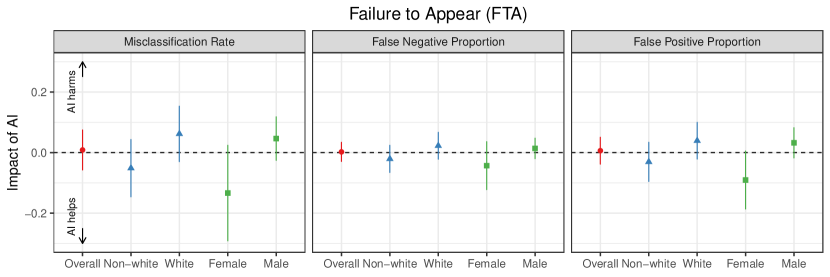
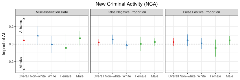
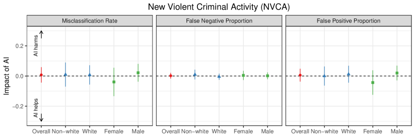
Figure 1: Estimated Impact of AI Recommendations on Human Decisions. The figure shows how AI recommendations improve a human judge’s cash bail decisions in terms of misclassification rate, false negative proportion, and false positive proportion. Each panel presents the overall and subgroup-specific results for a different outcome variable. For each quantity of interest, we report a point estimate and its corresponding 95% confidence interval for the overall sample (red circle), non-white and white subgroups (blue triangle), and female and male subgroups (green square). The results show that AI recommendations do not significantly improve the judge’s decisions.

Figure 1 presents the estimated impact of AI recommendations on human decisions in terms of the misclassification rate, proportion of false negatives, and proportion of false positives. We find that the AI recommendations do not significantly improve the judge’s decisions. Indeed, none of the classification risk differences between the judge’s decisions with and without the AI recommendations are statistically significant.

3.3 AI-alone decisions are less accurate than human decisions

Next, we compare the classification performance of AI-alone decisions with that of human decisions. Specifically, we estimate the upper and lower bounds of the differences in misclassification rate, false negative proportion, and false positive proportion between AI-alone and human decisions (with and without AI recommendations) using the partial identification results in Section 2.4. We obtain our estimates based on the sample analogues of parameters in these bounds and use a nonparametric bootstrap to compute the 95% confidence intervals.

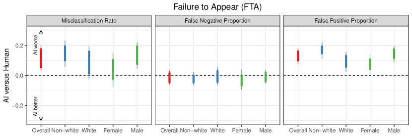
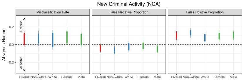
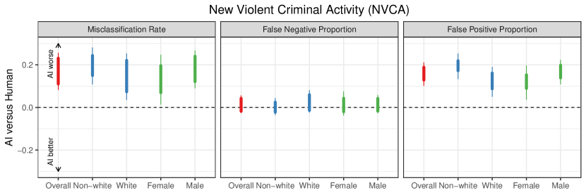
Figure 2: Estimated Bounds on Difference in Classification Ability between AI-alone and Human-alone Decisions. The figure shows misclassification rate, false negative proportion, and false positive proportion. Each panel presents the overall and subgroup-specific results for a different outcome variable. For each quantity of interest, we report estimated bounds (thick lines) and their corresponding 95% confidence interval (thin lines) for the overall sample (red), non-white and white subgroups (blue), and female and male subgroups (green). The results indicate that AI-alone decisions are less accurate than human judge’s decisions in terms of the false positive proportion.

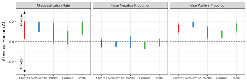
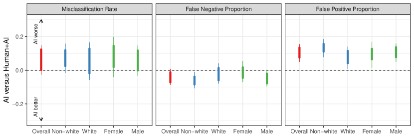
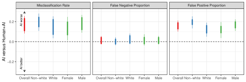
Figure S1: Estimated Bounds on Difference in Classification Ability between AI-alone and Human-with-AI Decision Making Systems. The figure shows misclassification rate, false negative proportion, and false positive proportion. Each panel presents the overall and subgroup-specific results for a different outcome variable. For each quantity of interest, we report estimated bounds (thick lines) and their corresponding 95% confidence interval (thin lines) for the overall sample (red), non-white and white subgroups (blue), and female and male subgroups (green). The results indicate that AI-alone decisions are less accurate than human judge’s decisions with AI recommendations in terms of the false positive proportion.

Figure 2 shows that the AI-alone system results in substantially higher false positive proportions, in comparison to the judge’s decisions regardless of whether or not the judge is given AI recommendations. This finding holds across the overall sample and within each subgroup, for each outcome variable. Qualitatively similar results are obtained when comparing the AI-alone and human-with-AI systems (see Figure S1 in Appendix S6). The results suggest that the AI system is generally harsher than the human judge, resulting in more cash bail decisions across subgroups and different outcome variables. This pattern is particularly strong for non-white arrestees where the AI system exhibits a large false positive proportion and hence misclassification rate that are both statistically significant (see Section 3.5).

For the false negative proportion, the differences between the AI-alone and human-alone systems are generally not statistically significant. However, for non-white arrestees with NCA as the outcome, AI-alone decisions have a lower false negative proportion than human-alone decisions, suggesting that human decisions are more lenient for this subgroup than AI-alone decisions. In sum, our analysis shows that when compared to human decisions, the AI-alone decision-making system is likely to result in a higher number of false positives, i.e., a greater number of cash bail decisions.

3.4 Human decisions are preferred over AI-alone system when the cost of false positives is high

Next, we analyze how one’s loss function determines their preference over different decision-making systems. Specifically, we follow the discussion at the end of Section 2.4 and invert the hypothesis test using the bounds on the difference in classification risk derived in Theorem 2. This analysis allows us to estimate the range of the loss of false positive ($\ell_{01}$), relative to the loss of false negative, that would lead us to prefer human decisions over the AI-alone system.

We invert the hypothesis test shown in Equation (10) over the range of values, $\ell_{01}\in[0.01,100]$ using the $0.05$ significance level. Specifically, for each candidate value of $\ell_{01}$, we conduct two one-sided hypothesis tests; one right-tailed and the other left-tailed, using the $t$-statistics of the lower and upper bounds of the difference in misclassification rates, respectively. If the right-tailed test null hypothesis, $H_{0}:U_{0}\geq 0$, is rejected (and thus the left-tailed test is not), we can conclude that the classification risk of the AI-alone system is likely greater than that of human decisions, suggesting a preference for human decisions over the AI-alone system. Conversely, if the left-tailed test of null hypothesis $H_{0}:L_{0}\leq 0$ is rejected, it indicates a preference for the AI-alone system. If neither test is rejected, we conclude that the preference between the decision-making systems is ambiguous.

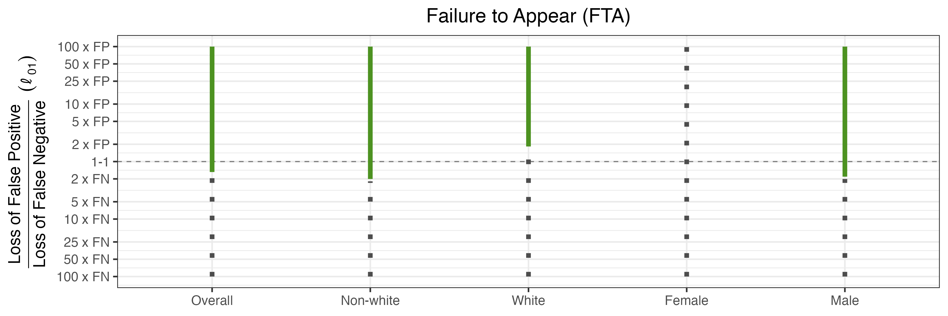
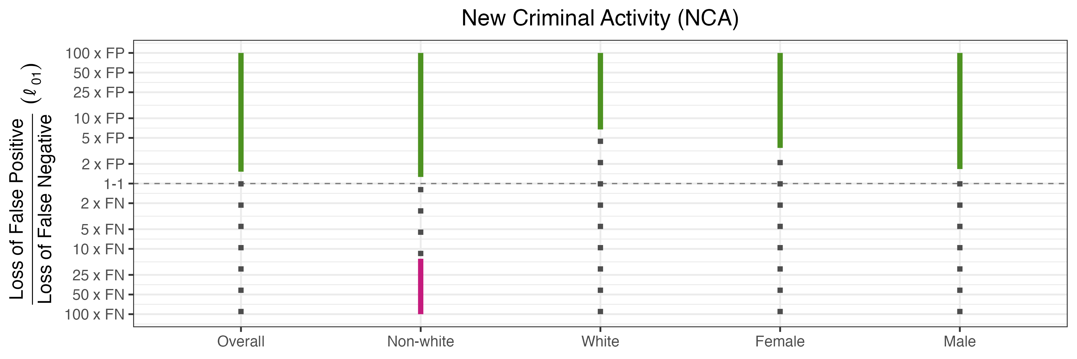
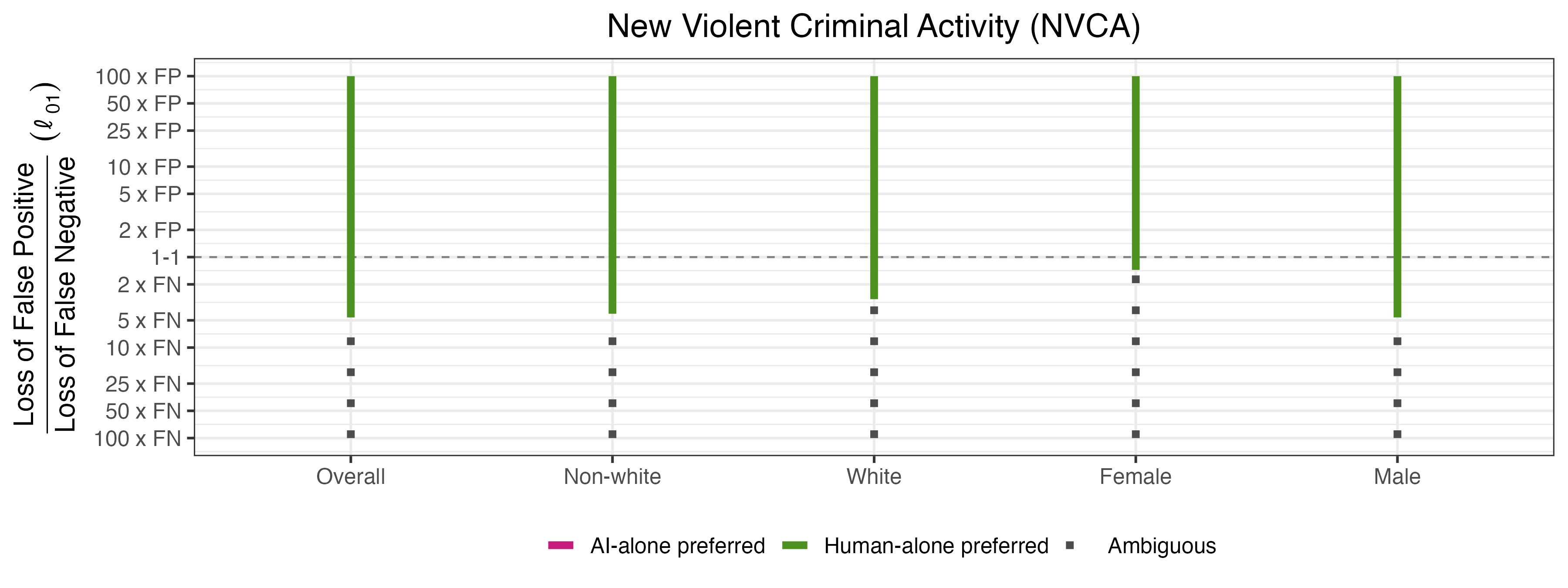
Figure 3: Estimated Preference for Human-alone Decisions over AI-alone Decision-Making System. The figure illustrates the range of the ratio of the loss between false positives and false negatives, $\ell_{01}$, for which one decision-making system is preferable over the other. A greater value of the ratio $\ell_{01}$ implies a greater loss of false positive relative to that of false negative. Each panel displays the overall and subgroup-specific results for different outcome variables. For each quantity of interest, we show the range of $\ell_{01}$ that corresponds to the preferred decision-making system; AI-alone (pink lines), human-alone (green lines), and ambiguous (dotted lines). The results suggest that the human-alone system is preferred over the AI-alone system when the loss of false positive is about the same as or greater than that of false negative.

Figure 3 shows that the human-alone system is preferred over the AI-alone system when the loss of false positive is about the same as or greater than that of false negative. For instance, with FTA as an outcome, the human-alone system is preferred over the AI-alone system when $\ell_{01}\geq 0.66$. Similar results are observed across various outcomes and subgroups, particularly for NVCA, where we find that the human-alone system is preferred when $\ell_{01}\geq 0.22$.

An exception is the finding for female arrestees that when FTA is the outcome the results are ambiguous. This is consistent with the finding that for female arrestees there exists a relatively small difference in the false positive and false negative proportions between the two systems (see Figure 2). Another exception is the finding that for NCA, the AI system is preferred over the human-alone system for non-white arrestees when the cost of false negative is weighted more heavily than that of false positive ($\ell_{01}\leq 0.07$). This is because, as shown in Figure 2, the AI system shows a smaller false negative proportion for non-whites than human-alone decisions when NCA is the outcome.

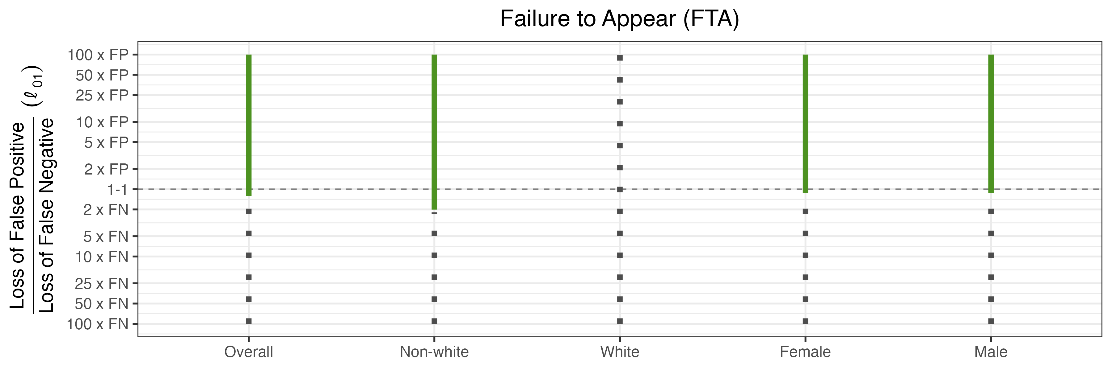
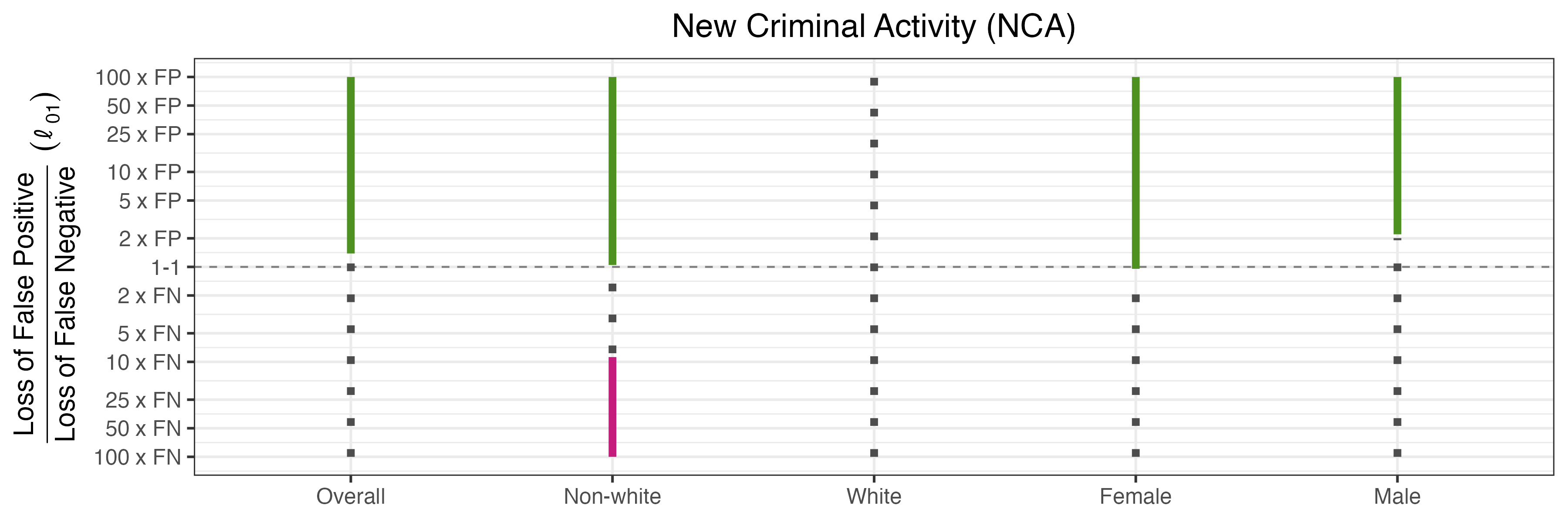
Figure S2: Estimated Preference for Human-with-AI over AI Decision-Making Systems. The figure illustrates the range of the ratio of the loss between false positives and false negatives, $\ell_{01}$, at which one can conclude that one decision-making system is preferable to the other. The higher the ratio (i.e. located at the top of the figure), the greater the loss from false positives compared to that from false negatives. Each panel displays the overall and subgroup-specific results for different outcome variables. For each quantity of interest, we show the range of $\ell_{01}$ where AI is preferred (pink lines), where the human-alone system is preferred (green lines), and where the preference is ambiguous (dotted lines). The results suggest that the human-alone system is preferred over the AI-alone system when the loss from false positives is about the same as or outweighs that from false negatives.

Qualitatively similar results are also obtained when comparing the AI-alone and human-with-AI systems (see Figure S2 in Appendix S6), though we observe ambiguous results for white arrestees with either FTA and NCA as an outcome. These results suggest that the human-alone system is preferred over the AI-alone system for a wide range of loss ratio.

3.5 AI-alone decisions result in more false positives for non-white arrestees

Finally, we compare the difference in classification performance between white and non-white arrestees under the AI-alone and human-alone decision making systems. The key idea is that conditional on the baseline potential outcome $Y(0)$, the decision should not depend on the race of an individual. Thus, two individuals for whom $Y(0)=0$, one white and one non-white, should receive the same decision under either a human-alone or AI-alone system.

As discussed in Section 2.2, this approach to racial disparity estimation has an important limitation in that it only focuses on the baseline potential outcome $Y(0)$ and ignores the other potential outcome $Y(1)$. Under the current framework, a signature bond decision on anyone with $Y(0)=1$ is regarded as a false negative, but it is possible that an individual with $Y(0)=1$ would engage in misconduct under a cash bail decision, i.e., $Y(1)=1$. A jurisdiction may have good reasons to prefer different decisions for these two types of arrestees, i.e., $(Y(0),Y(1))=(1,0),(1,1)$. Imai et al. (2023a) conduct such an analysis, albeit requiring a stronger assumption.

Proceeding with this limitation in mind, when point-identification is not possible, we estimate the lower and upper bounds of the quantities of interest, using the partial identification results presented in Section 2.4. We can point identify racial disparity in the proportion of false negatives under the human-alone and human-with-AI systems. All the other quantities are only partially identified.

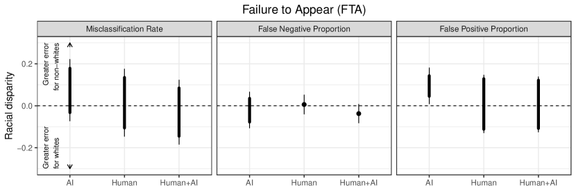
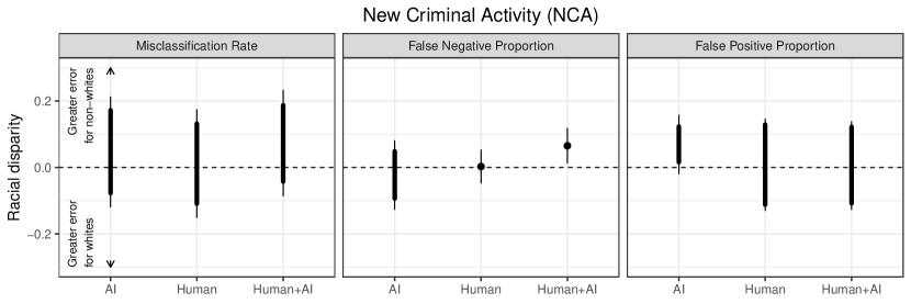
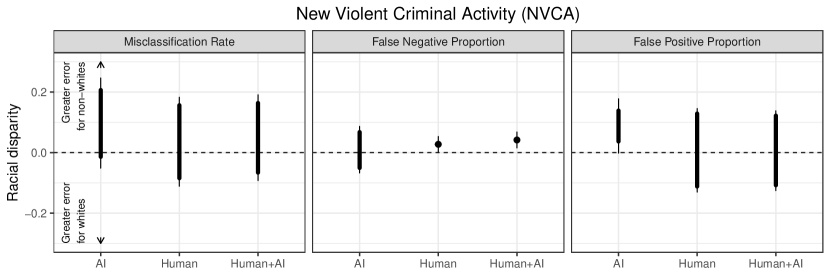
Figure 4: Estimated Racial Disparity under Each Decision-Making System. The figure shows the differences in the misclassification rate, false negative proportion, and false positive proportion between non-white and white arrestees under each decision-making system. Each panel displays the racial disparity in AI-alone, human-alone, and human-with-AI systems for different outcome variables. For each quantity of interest, we present estimated bounds (thick lines), point estimates (circles; specifically for the false negative proportion in human-alone and human-with-AI systems), and their corresponding 95% confidence intervals (thin lines). The results indicate that AI recommendations tend to yield more false positives for non-white arrestees.

Figure 4 shows that the AI-alone system may yield more false positives for non-white arrestees than white arrestees. This result is, however, only marginally significant when FTA is considered as an outcome, and it is not statistically significant for NVCA. This finding indicates that the AI system may be more likely to impose cash bail on a non-white arrestee than a white arrestee even when both of them would not engage in misconduct if they were to be released upon their own recognizance. For the human-alone and human-with-AI systems, we find no statistically significant racial difference in false positive proportion. There appears to be some differences in false negative proportion, but the magnitude of these differences is small and some of them are not statistically significant. Finally, we find no clear pattern in terms of racial difference in the overall misclassification rate.

4 Concluding Remarks

We have introduced a new methodological framework that provides a way to evaluate experimentally the performance of three different decision-making systems: human-alone, AI-alone, and human-with-AI systems. We formalized the classification ability of each decision-making system using standard confusion matrices based on potential outcomes. We then showed that under single-blinded randomization of treatment assignment, we can directly identify the differences in classification ability between human decision-makers with and without AI recommendations. Furthermore, we derived partial identification bounds to compare the differences in classification ability between an AI-alone and human decision-making systems and separately evaluate the performance of each system.

To illustrate the power of the proposed methodological framework, we apply our framework to the data from our own randomized controlled trial whose goal is to evaluate the impact of AI-generated risk assessment score on a judge’s decision to impose a cash bail or release arrestees on their own recognizance. We compare the human-alone and human-with-AI decisions and find little to no impact of AI recommendation. Our comparison of the human decision-maker with the AI-alone system suggests, based on the baseline potential outcome and around 40% of the RCT’s enrolled cases, that AI-alone decisions may underperform as compared to human decisions, resulting in a greater proportion of harsh decisions and differences in accuracy across racial groups for certain classification ability measures. All together, these empirical findings suggest that integrating AI recommendations into judicial decision-making warrants careful consideration and rigorous empirical evaluation.

There are several exciting future methodological research directions that can build on the current work. The proposed methodological framework can be extended to common settings where decisions and outcomes are non-binary. Another possible extension is the consideration of joint potential outcomes as done in Imai et al. (2023a) and the dynamic settings where multiple decisions and outcomes are observed over time. Finally, the proposed methodology and its extensions can be applied to a variety of real world settings where AI decision-making systems have been integrated or considered for future use.

Supplementary Appendix

Appendix S1 Generic Loss Functions

As a generic loss function, we can define separate weights for true positives $\ell_{11}$, true negatives $\ell_{00}$ and false positive $\ell_{01}$ so that the expected loss is given by $R(\ell_{00},\ell_{01},\ell_{11})=\ell_{10}q_{10}+\ell_{01}q_{01}+\ell_{11}q_{11}+\ell_{00}q_{00}$ with a proper normalization constraint such as $\ell_{10}=1$. All of the quantities we have considered in the main text are special cases of this generic loss function. For example, the difference in risk between the human-with-AI and human-alone systems is given by,

$$R_{\textsc{human+AI}}(\ell_{00},\ell_{01},\ell_{11})-R_{\textsc{human}}(\ell_{00},\ell_{01},\ell_{11})$$

$$= p_{10\cdot}(1)-p_{10\cdot}(0)+\ell_{01}(p_{01\cdot}(1)-p_{01\cdot}(0))+\ell_{11}\left(p_{11\cdot}(1)-p_{11\cdot}(0)\right)+\ell_{00}\left(p_{00\cdot}(1)-p_{00\cdot}(0)\right).$$

Now, recall that the false positive proportions under each system $(p_{01\cdot}(z)$ are not identified, but the difference is identifiable as $p_{01\cdot}(1)-p_{01\cdot}(0)=p_{00\cdot}(0)-p_{00\cdot}(1)$. We can similarly point identify the difference in true positive proportions as $p_{11\cdot}(1)-p_{11\cdot}(0)=p_{10\cdot}(0)-p_{10\cdot}(1)$. So, following the argument for Theorem 1, we can point identify the difference in risk with the generic loss function as:

$$R_{\textsc{human+AI}}(\ell_{00},\ell_{01},\ell_{11})-R_{\textsc{human}}(\ell_{00},\ell_{01},\ell_{11})$$

$$= (1-\ell_{11})\left(p_{10\cdot}(1)-p_{10\cdot}(0)\right)+(\ell_{00}-\ell_{01})\left(p_{00\cdot}(1)-p_{00\cdot}(0)\right).$$

We can similarly evaluate the human-with-AI vs AI-alone and human-alone vs AI-alone systems by following the partial identification arguments in Section 2.4, and evaluate the decision-making systems independently directly using Theorem S1 in Section S4.

Appendix S2 Connection to the Average Principal Causal Effects

Here, we discuss the connection between the proposed measures of ability and the average principal causal effects (APCE) introduced in Imai et al. (2023a). The authors consider a principal stratification setup based on the joint potential outcomes under the single-blinded experimental design. Specifically, under their framework, there are three principal strata: (1) preventable cases $(Y(1),Y(0))=(0,1)$)—individuals who engage in misconduct if released, and do not if detained, (2) risky cases $(Y(1),Y(0))=(1,1)$)– individuals who engage in misconduct, regardless of the judge’s decision, and (3) safe cases $(Y(1),Y(0)=(0,0)$)–i.e., individuals who would engage in misconduct, regardless of the detention decision. The remaining principal strata $(Y(1),Y(0))=(1,0)$ does not exist if the strong monotonicity assumption, i.e., $Y_{i}(1)=0$ for all $i$, holds; individuals would never engage in misconduct if detained.

Imai et al. focus on the average treatment effects across the preventable and safe cases to evaluate the impact of AI recommendations on human decisions. These Average Principal Causal Effects (APCEs) are defined as:

APCEp $$= \mathbb{E}\{D(1)-D(0)\mid Y(0)=1,Y(1)=0\},$$

APCEs $$= \mathbb{E}\{D(1)-D(0)\mid Y(0)=0,Y(1)=0\},$$

respectively. Under the strong monotonicity assumption, we can write these APCEs as:

APCEp $$= \frac{p_{10\cdot}(1)}{p_{10\cdot}(1)+p_{11\cdot}(1)}-\frac{p_{10\cdot}(0)}{p_{10\cdot}(0)+p_{11\cdot}(0)},$$

APCEs $$= \frac{p_{01\cdot}(1)}{p_{00\cdot}(1)+p_{01\cdot}(1)}-\frac{p_{01\cdot}(0)}{p_{00\cdot}(0)+p_{01\cdot}(0)}.$$

Therefore, under strong monotonicity, APCEp is equal to the difference in false positive rates between human-with-AI and systems, and APCEs is equal to the difference in false negative rates between the two systems.

Appendix S3 Bounds on Other Classification Ability Measures

In this appendix, for completeness, we present the bounds for other classification ability measures.

Proposition S1

(Bounds on false negative rate (FNR), false positive rate (FPR), and false discovery rate (FDR))

1. Human-alone system $(z=0)$ and Human-with-AI system ($z=1$):

   $$\frac{\Pr(Y=1,D=0\mid Z=z)}{\Pr(Y=1,D=0\mid Z=z)+\overline{p}_{11\cdot}(z)}\ \leq\text{FNR}(z) :=\frac{p_{10\cdot}(z)}{p_{1\cdot\cdot}(z)}\leq\frac{\Pr(Y=1,D=0\mid Z=z)}{\Pr(Y=1,D=0\mid Z=z)+\underline{p}_{11\cdot}(z)}$$

   $$\frac{\underline{p}_{01\cdot}(z)}{\Pr(Y=0,D=0\mid Z=z)+\overline{p}_{01\cdot}(z)}\ \leq\ \text{FPR}(z) :=\frac{p_{01\cdot}(z)}{p_{0\cdot\cdot}(z)}\ \leq\ \frac{\overline{p}_{01\cdot}(z)}{\Pr(Y=0,D=0\mid Z=z)+\underline{p}_{01\cdot}(z)},$$

   $$\frac{\underline{p}_{01\cdot}(z)}{\Pr(D=1\mid Z=z)}\ \leq\ \text{FDR}(z) :=\frac{p_{01\cdot}(z)}{\Pr(D(z)=1)}\ \leq\ \frac{\overline{p}_{01\cdot}(z)}{\Pr(D=1\mid Z=z)},$$

   where $[\underline{p}_{y1\cdot}(z),\overline{p}_{y1\cdot}(z)]:=[0,\Pr(D=1\mid Z=z)]$, for $y\in\{0,1\}$.

2. AI-alone system:

   $$\frac{\min_{z\in\{0,1\}}\{\underline{p}_{110}(z)+p_{100}(z)\}}{\max_{z\in\{0,1\}}\left\{p_{10\cdot}(z)+\overline{p}_{11\cdot}(z)\right\}}\ \leq\ \text{FNR}_{\textsc{AI}} :=\frac{p_{1\cdot 0}(z)}{p_{1\cdot\cdot}(z)}\ \leq\ \frac{\max_{z\in\{0,1\}}\left\{\overline{p}_{110}(z)+p_{100}(z)\right\}}{\min_{z\in\{0,1\}}\left\{p_{10\cdot}(z)+\underline{p}_{11\cdot}(z)\right\}},$$

   $$\frac{\min_{z\in\{0,1\}}\{p_{001}(z)+\underline{p}_{011}(z)\}}{\max_{z\in\{0,1\}}\left\{p_{10\cdot}(z)+\overline{p}_{11\cdot}(z)\right\}}\ \leq\ \text{FPR}_{\textsc{AI}} :=\frac{p_{001}(z)+p_{011}(z)}{p_{0\cdot\cdot}(z)}\ \leq\ \frac{\max_{z\in\{0,1\}}\{p_{001}(z)+\overline{p}_{011}(z)\}}{\min_{z\in\{0,1\}}\left\{p_{00\cdot}(z)+\underline{p}_{01\cdot}(z)\right\}}$$

   $$\frac{\min_{z\in\{0,1\}}\left\{p_{001}(z)+\underline{p}_{011}(z)\right\}}{\Pr(A=1)}\ \leq\ \text{FDR}_{\textsc{AI}} :=\frac{p_{001}(z)+p_{011}(z)}{p_{0\cdot 1}(z)+p_{1\cdot 1}(z)}\ \leq\ \frac{\max_{z\in\{0,1\}}\left\{p_{001}(z)+\overline{p}_{011}(z)\right\}}{\Pr(A=1)},$$

   where $p_{y0a}=\Pr(Y=y,D=0,A=a)$ for $y,a\in\{0,1\}$, and $\underline{p}_{y1a}$ and $\overline{p}_{y1a}$ are defined in Theorem 3.

Appendix S4 Point Identification based on the Assumption of Restricted Heterogeneity

In this appendix, we show that under two additional assumptions, it is possible to point-identify all elements of the confusion matrices and thereby any classification ability measures.

S4.1 Assumptions

Our first assumption is that AI recommendations affect human decisions, conditional on a set of pre-treatment covariates $X\in\mathcal{X}$ chosen by analysts.

Assumption 1

(Non-zero average effect of AI recommendations on human decisions within each strata)

$$\Pr(D(1)=1\mid X=x,A=a)\ \neq\ \Pr(D(0)=1\mid X=x,A=a)\quad\text{for all }x\in\mathcal{X},\ a\in\{0,1\}.$$

In our application, the assumption implies that the judge’s access to the AI recommendation must impact, on average, their decisions, after conditioning on $X$. The choice of $X$ is important. For example, the assumption will be violated if a judge systematically ignores the AI recommendation for a subset of cases defined by the covariates $X$. In general, if $X$ is high-dimensional, this assumption is unlikely to hold because there may exist some values of $X$ for which the AI recommendation does not systematically affect human decisions. Fortunately, under our proposed single-blinded experimental design, analysts can check the plausibility of this assumption by investigating whether or not the observed decision $D$ is independent of randomized treatment assignment $Z$ conditional on the covariates, $X$.

The second assumption states that conditional on the same set of pre-treatment covariates $X$ used in Assumption 1, the individual effects of AI recommendations on human decisions are unrelated to the baseline potential outcome $Y(0)$.

Assumption 2

(Restricted heterogeneous effects of AI recommendation on human decisions)

$$D(1)-D(0)\ \raisebox{0.50003pt}{\rotatebox[origin={c}]{90.0}{$\models$}}\ Y(0)\mid X=x,A=a\quad\text{for all }x\in\mathcal{X},\ a\in\{0,1\}.$$

Unlike Assumption 1, there is no direct observable implication of Assumption 2 because the restriction is placed on the joint distribution of the unit-level effect and the baseline potential outcome, which is not identifiable from the observed data. Assumptions about effect heterogeneity similar to Assumption 2 has been studied in the literature on instrumental variables (e.g., Chen et al., 2023; Wang and Tchetgen Tchetgen, 2018).

Assumption 2 is violated if within each strata defined by $X$ the probability of AI recommendations affecting human decisions depends on the baseline potential outcome. For example, suppose that a judge had additional information about the family support of arrestee, which changes how the AI recommendation affects their decision. Since the existence of family support is also likely to affect the baseline potential outcome, not including this information in $X$ will lead to the violation of Assumption 2. This may suggest that analysts should collect all relevant pre-treatment covariates and include them in $X$. As noted earlier, however, doing so may lead to the violation of Assumption 1 where human decision makers ignore AI recommendation for some values of $X$. This tradeoff underlies the fact that the choice of $X$ needs to be made with care.

S4.2 Identification

The next theorem shows that if these additional assumptions hold, we can identify all elements of confusion matrices and hence the risk of each decision-making system separately.

Theorem S1 (Identification of the confusion matrices)

Under Assumptions 1–2, each component of the confusion matrices, $C_{\textsc{Human}}(z)$ and $C_{\textsc{AI}}$ given in Equations (2) and (8), can be identified using the following equality:

$$p_{y1a}(z)\ =\ \mathbb{E}\left[\frac{p_{y0a}(1,X)-p_{y0a}(0,X)}{\Delta_{a}(X)}\right]-p_{y0a}(z),$$

for $y,a,z\in\{0,1\}$, and $\Delta_{a}(X):=e_{0}(X,a)-e_{1}(X,a)$.

Theorem S1 leverages the random provision of AI recommendation as an instrument, showing that conditional on $X$, the total proportion $\Pr(Y(0)=y,A=a\mid X=x)$ is equal to the difference in the proportion between the treatment and control groups divided by a $\Delta_{a}(X)$ term, which represents the difference in the decision rates from exposure to the AI. We will refer to $\Delta_{a}(X)$ as the AI-influence score. Under Assumption 2, the effect of AI recommendations on human decisions is independent of the baseline potential outcome. As such, we can scale the difference in the within-strata proportion of cases from exposure to the AI recommendations by the AI-influence score to recover the total proportion within the strata $X=x$.

An immediate implication of Theorem S1 is that we can identify the risk of each decision-making system by substituting the result of Theorem S1 into the definition of classification risk given in Equation (1). Similarly, we can identify all ability measures introduced in Section 2.2.

Corollary 1 (Identification of the classification risk of each decision-making system)

Under Assumptions 1–2, we can identify the risk of each decision-making system as follows:

$$R_{\textsc{AI}}(\ell_{01}) =\mathbb{E}\left[\frac{p_{100}(1,X)-p_{100}(0,X)}{\Delta_{0}(X)}+\ell_{01}\frac{p_{001}(1,X)-p_{001}(0,X)}{\Delta_{1}(X)}\right],$$

$$R_{\textsc{Human}}(\ell_{01}) =p_{10\cdot}(0)+\ell_{01}\left(\mathbb{E}\left[\frac{p_{10a}(1,X)-p_{y0a}(0,X)}{\Delta_{\boldsymbol{\cdot}}(X)}\right]-p_{00\cdot}(0)\right),$$

$$R_{\textsc{Human+AI}}(\ell_{01}) =p_{10\cdot}(1)+\ell_{01}\left(\mathbb{E}\left[\frac{p_{10a}(1,X)-p_{y0a}(0,X)}{\Delta_{\boldsymbol{\cdot}}(X)}\right]-p_{00\cdot}(1)\right),$$

where $\Delta_{a}(X):=\Pr(D(0)=1\mid X,A=a)-\Pr(D(1)=1\mid X,A=a)=\Pr(D=1\mid Z=0,X,A=a)-\Pr(D=1\mid Z=1,X,A=a)$, and $\Delta_{\boldsymbol{\cdot}}(X)$ is equivalently defined, but marginalizes over $A$.

To estimate the classification risk of a decision-making system in practice, we leverage a two-stage least squares approach to estimate $p_{y1a}(z)$, and use plug-in estimates for the observed quantities. To quantify the estimation uncertainty, we recommend researchers employ a percentile bootstrap approach. Alternatively, we can follow Wang and Tchetgen Tchetgen (2018) and use multiply robust estimation.

S4.3 Sensitivity analysis

While Assumptions 1 and 2 are powerful and enable us to identify all classification risk and ability measures under each decision-making system, they may not hold in practice. As discussed earlier, Assumption 2 cannot be directly verified using the data and also may be in conflict with Assumption 1. In addition, although Section 2.4 provides a way for researchers to partially identify the relevant quantities of interest, some of the bounds can be conservative.

To address this problem, we develop a sensitivity analysis that allows analysts to empirically examine the robustness of their risk and other ability measure estimates to the potential violation of Assumption 2 (while maintaining Assumption 1). As explained above, Assumption 2 may be violated if the conditioning variables $X$ do not have all the information available to the human decision-maker. As such, $\Delta_{a}(x)$ represents the observed AI-influence score within a strata $X=x$. We now define the oracle AI-influence score as follows:

$$\Delta^{*}_{ya}(x):= \mathbb{E}(D(0)-D(1)\mid X=x,A=a,Y(0)=y)$$

$$= \Pr(D(0)=1,D(1)=0\mid Y(0)=y,X=x,A=a)$$

$$~{}~{}~{}~{}~{}~{}~{}~{}~{}-\Pr(D(0)=0,D(1)=1\mid Y(0)=y,X=x,A=a),$$ (S1)

for $y,a\in\{0,1\}$ and $x\in\mathcal{X}$.

Note that $\Delta^{*}_{ya}(x)$ represents the differential impact of AI recommendations on human decisions for the cases $Y(0)=y$, conditional on the covariates $X=x$ and AI recommendation $A=a$. For example, the first term of $\Delta^{*}_{11}(x)$ represents the proportion of positive cases with AI recommendation of detention, in which a judge changes their decision from cash bail to release on one’s own recognizance because by going against the AI recommendation. In contrast, the second term represents the proportion of these cases, in which the a judge changes their decision by following the AI recommendation.

Thus, $\Delta^{*}_{ya}(x)$ represents the difference between these two proportions. In general, we expect that the sign of $\Delta^{*}_{ya}(x)$ should align with the observed AI-influence score $\Delta_{a}(x)$. This arises from the fact that in practice, we can assume that human decision-makers will not defy the AI recommendation. This implicitly constrains the sign of $\Delta^{*}_{ya}(x)$. In particular, we will expect $\Delta_{y1}(x)\leq 0$ and $\Delta_{y0}(x)\geq 0$ for all $y\in\{0,1\}$ and $x\in\mathcal{X}$. The no-defier assumption can be checked using observed data. For example, consider $A=1$. Then,

$$\Delta_{1}(X): =e_{0}(X,A=1)-e_{1}(X,A=1)$$

$$=\Pr(D(0)-D(1)=1\mid X,A=1)-\Pr(D(0)-D(1)=-1\mid X,A=1)$$

$$=-\Pr(D(0)-D(1)=-1\mid X,A=1)<0.$$

This follows from the fact that $\Pr(D(0)-D(1)=1\mid X,A=1)=0$, as we have ruled out the scenario in which the decision-maker initially had a decision of $D(0)=1$, but upon seeing the AI recommendation of $A=1$, flipped their decision to be contrarian to the AI recommendation. We can actually directly check this to see if $\Delta_{1}(X)<0$. Similarly, we can check to see if $\Delta_{0}(X)>0$ for cases in which $A=0$.

Under Assumption 2, the baseline outcome $Y(0)$ will be independent of $D(0)-D(1)$. This means that $\Delta^{*}_{ya}(x)$ will equal to the average effect of AI recommendations on human decisions, i.e., $\Delta^{*}_{ya}(x)=\Delta_{a}(x)$ for all $y,a\in\{0,1\}$ and $x\in\mathcal{X}$.

To conduct the sensitivity analysis, we define the following uncertainty set for $\Delta^{*}_{ya}(x)$.

Assumption 3 ($\epsilon$-constrained Confounding)

For $y\in\{0,1\}$ and $a\in\{0,1\}$, there exists $\epsilon_{L}>0$ and $\epsilon_{U}>0$ such that

$$\Delta^{*}_{ya}(x)\in\big{[}\Delta_{a}(x)-\epsilon_{L},\Delta_{a}(x)+\epsilon_{U}\big{]}\text{ for all }x\in\mathcal{X}.$$ (S2)

Assumption 3 constrains $\Delta^{*}_{ya}(x)$ to be within an $\epsilon_{L}+\epsilon_{U}$ neighborhood around the estimated $\Delta_{a}(x)$, for each strata $X=x$.

Our formulation of the uncertainty set allows researchers to consider asymmetric impacts of the omitted confounder. This is important because in practice, there are substantive implications for the directional impact of omitting a confounder. For example, consider $y=1$. If $\Delta_{1a}(x,a)>\Delta_{a}(x)$, this implies that we have overestimated TPP (i.e., $\Pr(Y(0)=1,D(z)=1\mid X=x,A=a)$). The overestimation arises because access to the AI recommendation resulted in more false decisions than the observed impact. In contrast, if $\Delta_{1a}(x)<\Delta_{a}(x)$, then this implies that the AI recommendation resulted in fewer incorrect decisions than the observed impact, and as a result, we have underestimated TPP. In settings when researchers have no strong prior for the directional impact of the omitted confounder, they can choose to set $\epsilon=\epsilon_{L}=\epsilon_{U}$.

When Assumption 2 is violated, the resulting estimate will be biased, depending on how different $\Delta^{*}_{ya}(x)$ is to the observed AI-influence score (i.e., $\Delta_{a}(x)$). As the size of the uncertainty set (i.e., $\epsilon_{L}+\epsilon_{U}$) increases, this implies that $\Delta^{*}_{ya}(x)$ deviates by a larger degree from the observed impact on decision-making. In the setting in which $\epsilon_{L}=\epsilon_{U}=0$, then this implies the assumption of restricted heterogeneity (Assumption 2) holds.

Given a fixed $\{\epsilon_{L},\epsilon_{U}\}$, we can then partially identify the risk under the potential violation of Assumption 2.

Proposition S2 (Adjusted Risk under Violations of Assumption 2)

Under Assumption 1 and $\epsilon$-constrained confounding (Assumption 3), $p_{y1a}(z,x)$ can be partially identified:

$$p_{y1a}(z,x)\in\left[\underline{p}_{y1a}(z,x;\epsilon_{L}),\overline{p}_{y1a}(z,x;\epsilon_{U})\right],$$

where the lower bound, $\underline{p}_{y1a}(z,x;\epsilon_{U})$, is defined as

$$\underline{p}_{y1a}(z,x;\epsilon):=\begin{cases}\displaystyle\frac{p_{y0a}(1,x)-p_{y0a}(0,x)}{\Delta_{a}(x)+\epsilon_{U}}-p_{y0a}(0,x)&\text{if }\epsilon_{U}<\overline{\Delta}_{ya}(x)-\Delta_{a}(x)\\ \max\left\{p_{y0a}(1,x)-2p_{y0a}(0,x),0\right\}&\text{if }\epsilon_{U}\geq\overline{\Delta}_{ya}(x)-\Delta_{a}(x),\end{cases}$$ (S3)

and the upper bound, $\overline{p}_{y1a}(z,x;\epsilon_{U})$, is defined as

$$\overline{p}_{y1a}(z,x;\epsilon):=\begin{cases}\displaystyle\frac{p_{y0a}(1,x)-p_{y0a}(0,x)}{\Delta_{a}(x)-\epsilon_{L}}-p_{y0a}(0,x)&\text{if }\epsilon_{L}<\underline{\Delta}_{ya}(x)-\Delta_{a}(x)\\ e_{z}(x,a)\cdot\Pr(A=a\mid X=x)&\text{if }\epsilon_{U}\geq\underline{\Delta}_{ya}(x)-\Delta_{a}(x).\end{cases}$$ (S4)

The lower and upper bounds on $\Delta^{*}_{ya}(x)$, denoted by $\underline{\Delta}_{ya}(x)$ and $\overline{\Delta}_{ya}(x)$ respectively, are given by:

$$\underline{\Delta}_{ya}(x):=\frac{p_{y0a}(1,x)-p_{y0a}(0,x)}{p_{y0a}(0,x)+e_{z}(x,a)\cdot\Pr(A=a\mid X=x)},\quad\overline{\Delta}_{ya}(x):=\min\left\{\frac{p_{y0a}(1,x)-p_{y0a}(0,x)}{p_{y0a}(0,x)},1\right\}.$$

Then, the adjusted risk under violations of Assumption 2 can be computed by using Equations (S3) and (S4).

Researchers can vary $(\epsilon_{L},\epsilon_{U})$ and estimate the range off possible risk values under the potential violation of Assumption 2. As $\epsilon_{L}$ and $\epsilon_{U}$ increase to more extreme values, we will recover the endpoints of the partially identified region (i.e., Theorem 2). The sensitivity analysis thus provides a helpful intermediary between point identification (i.e., Theorem S1) and an assumption-agnostic partial identification approach (i.e., Theorem 2).

Appendix S5 Proofs

With the exception of Theorem 2, we will present the proofs in the order that the theorems and corollaries appear in the paper.

S5.1 Proof of Theorem 1

Proof.

Under law of total probability,

$$p_{y\cdot\cdot}(z)=p_{y1\cdot}(z)+p_{y0\cdot}(z),\text{ for }z\in\{0,1\}.$$

Then, under random treatment assignment $Z$, $p_{y\cdot\cdot}(1)=p_{y\cdot\cdot}(0)$. As a result:

$$p_{y1\cdot}(1)+p_{y0\cdot}(1)=p_{y1\cdot}(0)+p_{y0\cdot}(0)\implies p_{y1\cdot}(1)-p_{y1\cdot}(0)=p_{y0\cdot}(0)-p_{y0\cdot}(1),$$

for $y\in\{0,1\}$. Then:

$$R_{\textsc{human+AI}}(\ell_{01})-R_{\textsc{human}}(\ell_{01}) =p_{10\cdot}(1)+\ell_{01}p_{01\cdot}(1)-\big{(}p_{10\cdot}(0)+\ell_{01}p_{01\cdot}(0)\big{)}$$

$$=p_{10\cdot}(1)-p_{10\cdot}(0)+\ell_{01}\times\big{(}p_{01\cdot}(1)-p_{01\cdot}(0)\big{)}$$

$$=p_{10\cdot}(1)-p_{10\cdot}(0)-\ell_{01}\times\big{(}p_{00\cdot}(1)-p_{00\cdot}(0)\big{)}$$

∎

S5.2 Proof of Theorem S1

Proof.

Because $p_{y0a}(z,x)$ are directly observed in the data, we focus on identification for $p_{y1a}(z,x)$. As an outline of the proof, we will first leverage the results from Chen et al. (2023) and Wang and Tchetgen Tchetgen (2018) to show that with a random instrument $Z$, we can identify the total proportion of cases $Y(0)=y$, for a strata. This then allows us to directly solve for $p_{y1a}(z,x)$.

From Theorem 1 of Chen et al. (2023), under Assumptions 1-2, we can identify $p_{y\cdot a}(z,x)$. To begin:

$$\mathbb{E} (\mathbbm{1}\{Y(0)=y\}\mid X=x,A=a)$$

$$= \frac{\text{cov}((1-D)\mathbbm{1}\{Y(0)=y\},Z\mid X=x,A=a)}{\text{cov}(1-D,Z\mid X=x,A=a)}$$

$$= \frac{\mathbb{E}(\mathbbm{1}\{Y(0)=y\}\mid D=0,Z=1,X=x,A=a)\Pr(D=0\mid Z=1,X=x)}{\Pr(D=0\mid Z=1,X=x,A=a)-\Pr(D=0\mid Z=0,X=x,A=a)}$$

$$\quad-\frac{\mathbb{E}(\mathbbm{1}\{Y(0)=y\}\mid D=0,Z=0,X=x,A=a)\Pr(D=0\mid Z=0,X=x,A=a)}{\Pr(D=0\mid Z=1,X=x,A=a)-\Pr(D=0\mid Z=0,X=x,A=a)}$$

$$= \frac{\Pr(Y(0)=y,D(1)=0\mid X=x,A=a,Z=1)-\Pr(Y(0)=y,D(0)=0\mid X=x,A=a,Z=0)}{\Pr(D(1)=0\mid X=x,A=a,Z=1)-\Pr(D(0)=0\mid X=x,A=a,Z=0)}$$

This implies that

$$p_{y\cdot a}(z,x)=\frac{p_{y0a}(1,x)-p_{y0a}(0,x)}{e_{0}(x,a)-e_{1}(x,a)},$$ (S5)

for $z=0,1$. Then, by Law of Total Probability:

$$p_{y\cdot a}(1,x) =p_{y1a}(1,x)+p_{y0a}(1,x),$$ (S6)

$$p_{y\cdot a}(0,x) =p_{y1a}(0,x)+p_{y0a}(0,x).$$ (S7)

Under Assumption 1, $p_{y\cdot a}(1,x)=p_{y\cdot a}(0,x)\equiv\mathbb{E}(\mathbbm{1}\{Y(0)=y\}\mathbbm{1}\{A=a\}\mid X=x)$. Thus, we can directly substitute Equation (S5) into Equations (S6) and (S7) to solve for $p_{y1a}(1,x)$ and $p_{y1a}(0,x)$:

$$p_{y1a}(1,x) =\frac{p_{y0a}(1,x)-p_{y0a}(0,x)}{e_{0}(x)-e_{1}(x)}-p_{y0a}(1,x)$$

$$p_{y1a}(0,x) =\frac{p_{y0a}(1,x)-p_{y0a}(0,x)}{e_{0}(x)-e_{1}(x)}-p_{y0a}(0,x)$$

Then, taking the expectation over all strata $X=x$:

$$p_{y1a}(z) =\mathbb{E}_{X}\left[\frac{p_{y0a}(1,X)-p_{y0a}(0,X)}{e_{0}(X)-e_{1}(X)}-p_{y0a}(z,X)\right]$$

$$=\mathbb{E}_{X}\left[\frac{p_{y0a}(1,X)-p_{y0a}(0,X)}{e_{0}(X)-e_{1}(X)}\right]-p_{y0a}(z)$$

for $z=0,1$, which concludes the proof. ∎

S5.3 Proof of Corollary 1

Proof.

We apply the results from Theorem S1 to identify the risk of each decision-making system. We begin with the AI-only system:

$$R_{\textsc{AI}}(\ell_{01}) =\sum_{z\in\{0,1\}}\big{(}p_{1\cdot 0}(z)+\ell_{01}\times p_{0\cdot 1}(z)\big{)}\Pr(Z=z)$$

$$=\sum_{z\in\{0,1\}}\mathbb{E}_{X}\left[\big{(}p_{1\cdot 0}(z,X)\right]+\ell_{01}\times\mathbb{E}_{X}\left[p_{0\cdot 1}(z,X)\right]\big{)}\Pr(Z=z)$$

$$=\mathbb{E}_{X}\left[\frac{p_{100}(1,X)-p_{100}(0,X)}{e_{0}(X,0)-e_{1}(X,0)}+\ell_{01}\times\left(\frac{p_{001}(1,X)-p_{001}(0,X)}{e_{0}(X,1)-e_{1}(X,1)}\right)\right]$$

For the human-only system:

$$R_{\textsc{Human}}(\ell_{01}) =p_{10\cdot}(0)+\ell_{01}\times p_{01\cdot}(0)$$

$$=p_{10\cdot}(0)+\ell_{01}\times\left(\mathbb{E}_{X}\left[\frac{p_{10a}(1,X)-p_{y0a}(0,X)}{e_{0}(X)-e_{1}(X)}\right]-p_{00\cdot}(0)\right)$$

Similarly, for the human-with-AI system:

$$R_{\textsc{Human+AI}}(\ell_{01}) =p_{10\cdot}(1)+\ell_{01}\times p_{01\cdot}(1)$$

$$=p_{10\cdot}(1)+\ell_{01}\times\left(\mathbb{E}_{X}\left[\frac{p_{10a}(1,X)-p_{y0a}(0,X)}{e_{0}(X)-e_{1}(X)}\right]-p_{00\cdot}(1)\right)$$

∎

S5.4 Proof of Proposition S2

Proof.

To prove Proposition S2, we will leverage three lemmas.

Lemma S1 (Bias under Violations of Restricted Heterogeneity)

Assume that Assumption 2 holds, given the set $\{X,U\}$ (i.e., $Y(0)\raisebox{0.50003pt}{\rotatebox[origin={c}]{90.0}{$\models$}}D(1)-D(0)\mid\{X,U\}$). Define $\lambda(U;X)$ and $\gamma(U;X)$ as follows:

$$\lambda(U;X)=\frac{\mathbb{E}(\mathbbm{1}\{Y(0)=y\}\mid X,U,A)}{\mathbb{E}(\mathbbm{1}\{Y(0)=y\}\mid X,A)}\ \ \text{and}\ \ \ \gamma(U;X)=\frac{e_{0}(X,U,A)-e_{1}(X,U,A)}{e_{0}(X,A)-e_{1}(X,A)}.$$

Then, $\mathbb{E}(\mathbbm{1}\{Y(0)=y\}\mathbbm{1}\{A=a\}\mid X=x)$ can be written as a function of $\lambda(U;X)$ and $\gamma(U;X)$:

$$\mathbb{E}(\mathbbm{1}\{Y(0)=y\}\mathbbm{1}\{A=a\}\mid X=x;\{\lambda,\gamma\})=\frac{1}{\mathbb{E}[\lambda(U;X)\gamma(U;X)\mid X]}\frac{p_{y0\cdot}(1,x)-p_{y0\cdot}(0,x)}{e_{0}(x)-e_{1}(x)}$$

Lemma S2 (Distribution of $D(0)-D(1)$)

Let $\delta_{cd}(X,A):=\Pr(D(1)=c\mid X,A,D(0)=d)$.

$$D(0)-D(1)=\begin{cases}-1&\Pr(D(0)-D(1)=-1\mid X,A)=e_{1}(X,A)-(1-\delta_{01}(X,A))e_{0}(X,A)\\ 0&\Pr(D(0)-D(1)=0\mid X,A)=1+e_{0}(X,A)-e_{1}(X,A)-2\cdot\delta_{01}(X,A)e_{0}(X,A)\\ 1&\Pr(D(0)-D(1)=1\mid X,A)=e_{0}(X,A)\delta_{01}(X,A)\end{cases}$$

Lemma S3 (Bounds of $\Delta^{*}_{ya}(x)$)

The bounds of the sensitivity parameter are given by,

$$\Delta^{*}_{ya}(x)\in[\underline{\Delta}_{ya}(x),\overline{\Delta}_{ya}(x)],$$

where

$$\underline{\Delta}_{ya}(x) :=\frac{p_{y0a}(1,x)-p_{y0a}(0,x)}{p_{y0a}(0,x)+e_{z}(x,a)\cdot\Pr(A=a\mid X=x)},$$

$$\overline{\Delta}_{ya}(x) :=\min\left\{\frac{p_{y0a}(1,x)-p_{y0a}(0,x)}{p_{y0a}(0,x)},1\right\}.$$

Applying the results of Lemma S1:

$$p_{y\cdot a}(z,x;\{\lambda,\gamma\})=\frac{1}{\mathbb{E}[\lambda(U;X)\gamma(U;X)\mid X,A]}\frac{p_{y0a}(1,x)-p_{y0a}(0,x)}{e_{0}(x,a)-e_{1}(x,a)}.$$ (S8)

Let $U:=Y(0)$.

$$\mathbb{E} \left[\lambda(U;X)\cdot\gamma(U;X)\mid X,A\right]$$

$$=\mathbb{E}\left[\left.\frac{\Pr(Y(0)=y\mid X,U,A)}{\Pr(Y(0)=y\mid X,A)}\cdot\frac{\mathbb{E}(D(0)-D(1)\mid X,U,A)}{\mathbb{E}(D(0)-D(1)\mid X,A)}\right|X,A\right]$$

$$=\mathbb{E}\left[\left.\frac{\Pr(Y(0)=y\mid X,A,Y(0)=y)}{\Pr(Y(0)=y\mid X,A)}\cdot\frac{\mathbb{E}(D(0)-D(1)\mid X,Y(0)=y,A)}{\mathbb{E}(D(0)-D(1)\mid X,A)}\right|X,A\right]$$

$$=\frac{\mathbb{E}(D(0)-D(1)\mid X,Y(0)=y,A)}{\mathbb{E}(D(0)-D(1)\mid X,A)}$$ (S9)

First, note that we can re-write $e_{0}(X,A)-e_{1}(X,A)$ as $\Pr(D(0)-D(1)=1\mid X,A)-\Pr(D(0)-D(1)=-1\mid X,A)$:

$$\mathbb{E}(D(0)-D(1)\mid X,A) =e_{0}(X,A)-e_{1}(X,A)$$ (S10)

$$=e_{0}(X,A)\delta_{01}(X,A)+(1-\delta_{01}(X,A))e_{0}(X,A))-e_{1}(X,A)$$

$$=e_{0}(X,A)\delta_{01}(X,A)-\big{(}e_{1}(X,A)-(1-\delta_{01}(X,A))e_{0}(X,A))$$

$$\equiv\Pr(D(0)-D(1)=1\mid X,A)-\Pr(D(0)-D(1)=-1\mid X,A)$$ (S11)

Similarly, $\mathbb{E}(D(0)-D(1)\mid X,Y(0)=y,A)=\Pr(D(0)-D(1)=1\mid X,A,Y(0)=y)-\Pr(D(0)-D(1)=-1\mid X,A)$.

$$\mathbb{E}\Big{[}\lambda(U;X)\cdot\gamma(U;X)\mid X,A\Big{]} \equiv\frac{\Pr(D(0)-D(1)=1\mid X,A,Y(0)=y)-\Pr(D(0)-D(1)=-1\mid X,A,Y(0)=y)}{\Pr(D(0)-D(1)=1\mid X,A)-\Pr(D(0)-D(1)=-1\mid X,A)}$$

Let $$\Delta^{*}_{ya}(x):=\Pr(D(0)-D(1)=1\mid Y(0)=y,X=x,A=a)-\Pr(D(0)-D(1)=-1\mid Y(0)=y,X=x,A=a)$$:

$$=\frac{\Delta^{*}_{ya}(x)}{\Pr(D(0)-D(1)\mid X,A)-\Pr(D(0)-D(1)=-1\mid X,A)}$$ (S12)

Finally, substituting Equation (S12) into Equation (S8):

$$p_{y\cdot a}(z,x;\Delta_{y})=\frac{p_{y0a}(1,x)-p_{y0a}(0,x)}{\Delta^{*}_{ya}(x)}$$

From Lemma S3, the possible range of $\Delta^{*}_{ya}(x)$ will be constrained to $[\underline{\Delta}_{ya}(x),\overline{\Delta}_{ya}(x)]$, where

$$\underline{\Delta}_{ya}(x):=\frac{p_{y0a}(1,x)-p_{y0a}(0,x)}{p_{y0a}(0,x)+e_{z}(x,a)\cdot\Pr(A=a\mid X=x)},$$

and

$$\overline{\Delta}_{ya}(x):=\min\left\{\frac{p_{y0a}(1,x)-p_{y0a}(0,x)}{p_{y0a}(0,x)},1\right\}.$$

This implicitly restricts $\epsilon_{L}$ and $\epsilon_{U}$. Thus, the results of the proposition immediately follow. ∎

S5.5 Proof of Theorem 2

Proof.

We are comparing the risk under an AI system, with the risk under a human decision-making system. To begin, we write $R_{\textsc{AI}}(\ell_{01})$ in terms of the different components of the confusion matrices. Because $p_{y\cdot a}(1)=p_{y\cdot a}(0)$ by randomness of $Z$ (i.e., Assumption 1, we can re-write the above with respect to just the treatment or control group:

$$R_{\textsc{AI}}(\ell_{01}) =p_{1\cdot 0}(0)+\ell_{01}\times p_{0\cdot 1}(0)$$

$$=p_{110}(0)+p_{100}(0)+\ell_{01}\times\left(p_{001}(0)+p_{011}(0)\right).$$

For $$R_{\textsc{Human}}(\ell_{01})$$:

$$R_{\textsc{Human}}(\ell_{01}) =p_{10\cdot}(0)+\ell_{01}\times p_{01\cdot}(0)$$

$$=p_{10\cdot}(0)+\ell_{01}\times\left(p_{010}(0)+p_{011}(0)\right).$$

Taking the difference between the two,

$$R_{\textsc{AI}} (\ell_{01})-R_{\textsc{Human}}(\ell_{01})$$

$$= p_{110}(0)+p_{100}(0)+\ell_{01}\times\left(p_{001}(0)+p_{011}(0)\right)$$

$$-\left[p_{10\cdot}(0)+\ell_{01}\times\left(p_{010}(0)+p_{011}(0)\right)\right]$$

$$= p_{110}(0)+p_{100}(0)+\ell_{01}\times p_{001}(0)-p_{10\cdot}(0)-\ell_{01}\times p_{010}(0)$$

$$= p_{110}(0)+\ell_{01}\times p_{001}(0)+p_{100}(0)-p_{10\cdot}(0)-\ell_{01}\times p_{010}(0)$$

$$= \underbrace{p_{110}(0)-\ell_{01}\times p_{010}(0)}_{\text{Unobserved}}-\underbrace{\big{(}p_{101}(0)-\ell_{01}\times p_{001}(0)\big{)}}_{\text{Observed}}.$$

Thus, to partially identify the difference in risk, we must bound $p_{110}(0)$ and $p_{010}(0)$. Generally, for $p_{y1a}(z)$, we have two constraints:

1. $p_{y1a}(z)\in[0,1-p_{y0a}(z)]$, which arises from $p_{y1a}(z)=p_{y\cdot a}(z)-p_{y0a}(z)$.

2. $p_{y1a}(z)\in[0,e_{z}(a)\Pr(A=a)]$, which arises from $p_{y1a}(z)=\Pr(Y(0)=y\mid D(z)=1,Z=z,A=a)\Pr(D(z)=1\mid A=a,Z=z)\Pr(A=a)$.

The second constraint is more restrictive than the first (i.e., $1-p_{y0a}(z)\geq e_{z}(a)\Pr(A=a)$):

$$p_{y0a}(z)+e_{z}(a)\Pr(A=a)=\Pr(Y(0)=y,D(z)=0,A=a)+\Pr(D(z)=1,A=a)\leq\Pr(A=a).$$

Thus, $p_{y1a}(z)\in[0,e_{z}(a)\Pr(A=a)]$ for $a,y,z=0,1$. The results of the theorem immediately follow. ∎

S5.6 Proof of Lemma S1

Proof.

For ease of notation, let $\tilde{D}=1-D$. If Assumption 2 is violated (i.e., $\text{cov}(\mathbb{E}(D(1)\mid X,U,A)-\mathbb{E}(D(0)\mid X,U,A),\mathbb{E}(\mathbbm{1}\{Y(0)=y\}\mid X,U,A))\neq 0$), then:

cov $$(\tilde{D}\mathbbm{1}\{Y(0)=y\},Z\mid X,A)-\mathbb{E}\big{[}\mathbb{E}(\mathbbm{1}\{Y(0)=y\}\mid X,U,A)\cdot\text{cov}(\tilde{D},Z\mid X,U,A)\mid X,A\big{]}$$

$$= \text{cov}(\tilde{D}\mathbbm{1}\{Y(0)=y\},Z\mid X,A)-\mathbb{E}(\mathbbm{1}\{Y(0)=y\}\mid X,A)\cdot\text{cov}(\tilde{D},Z\mid X,A)+$$

$$\underbrace{\mathbb{E}(\mathbbm{1}\{Y(0)=y\}\mid X,A)\cdot\text{cov}(\tilde{D},Z\mid X,A)-\mathbb{E}\big{[}\mathbb{E}(\mathbbm{1}\{Y(0)=y\}\mid X,U,A)\cdot\text{cov}(\tilde{D},Z\mid X,U,A)\mid X,A\big{]}}_{:=\xi}$$

$$= \text{cov}(\tilde{D}\mathbbm{1}\{Y(0)=y\},Z\mid X,A)-\mathbb{E}(\mathbbm{1}\{Y(0)=y\}\mid X,A)\cdot\text{cov}(\tilde{D},Z\mid X,A)+\xi=0$$

As such, when solving for $\mathbb{E}(\mathbbm{1}\{Y(0)=y\}\mid X,A)$, we have the following instead:

$$\mathbb{E}(\mathbbm{1}\{Y(0)=y\}\mid X,A)=\frac{\text{cov}(\tilde{D}\mathbbm{1}\{Y(0)=y\},Z\mid X,A)+\xi}{\text{cov}(\tilde{D},Z\mid X,A)},$$ (S13)

where $\xi$ is defined as follows:

$$\xi=\mathbb{E}(Y(0)\mid X,A)\cdot\text{cov}(\tilde{D},Z\mid X,A)-\mathbb{E}\big{[}\mathbb{E}(Y(0)\mid X,U,A)\cdot\text{cov}(\tilde{D},Z\mid X,U,A)\mid X,A\big{]}.$$

We can re-parameterize $\xi$:

$$\mathbb{E} (\mathbbm{1}\{Y(0)=y\}\mid X,A)\cdot\text{cov}(\tilde{D},Z\mid X,A)$$

$$=\mathbb{E}(\mathbbm{1}\{Y(0)=y\}\mid X,A)\left(\mathbb{E}(\tilde{D}Z\mid X,A)-\mathbb{E}(\tilde{D}\mid X,A)\mathbb{E}(Z\mid X,A)\right)$$

$$=\mathbb{E}(\mathbbm{1}\{Y(0)=y\}\mid X,A)\left(e_{0}(X,A)-e_{1}(X,A)\right)\cdot\text{var}(Z\mid X,A)$$

Similarly:

$$\mathbb{E} (Y(0)\mid X,U,A)\cdot\text{cov}(\tilde{D},Z\mid X,U,A)$$

$$=\mathbb{E}(Y(0)\mid X,U,A)\left(e_{0}(X,U,A)-e_{1}(X,U,A)\right)\text{var}(Z\mid X,A)$$

Then, define $\ lambda(U;X)$ and $\gamma(U;X)$ as:

$$\lambda(U;X): =\mathbb{E}(Y(0)\mid X,U,A)/\mathbb{E}(Y(0)\mid X,A),\text{ and}$$

$$\gamma(U;X): =(e_{0}(X,U,A)-e_{1}(X,U,A))/(e_{0}(X,A)-e_{1}(X,A)).$$

Then:

$$\xi= \mathbb{E}(\mathbbm{1}\{Y(0)=y\}\mid X,A)\cdot\text{cov}(\tilde{D},Z\mid X,A)$$

$$~{}~{}~{}-\mathbb{E}\big{[}\mathbb{E}(\mathbbm{1}\{Y(0)=y\}\mid X,U,A)\cdot\text{cov}(\tilde{D},Z\mid X,U,A)\mid X,A\big{]}$$

$$= \text{var}(Z\mid X,A)\times\Big{(}\mathbb{E}(\mathbbm{1}\{Y(0)=y\}\mid X,A)\left(e_{0}(X,A)-e_{1}(X,A)\right)$$

$$~{}~{}~{}~{}~{}~{}~{}~{}~{}~{}~{}~{}~{}~{}~{}~{}~{}~{}~{}~{}~{}~{}~{}~{}~{}~{}~{}~{}-\mathbb{E}(\mathbb{E}(\mathbbm{1}\{Y(0)=y\}\mid X,U,A)\cdot(e_{0}(X,U,A)-e_{1}(X,U,A))\Big{)}$$

$$= \text{var}(Z\mid X,A)\times\mathbb{E}(\mathbbm{1}\{Y(0)=y\}\mid X,A)(e_{0}(X,A)-e_{1}(X,A))\left(1-\mathbb{E}(\lambda(U;X)\cdot\gamma(U;X)\mid X,A)\right)$$ (S14)

Substituting Equation (S14) into Equation (S13):

$$\mathbb{E} (\mathbbm{1}\{Y(0)=y\}\mid X,A)$$

$$= \frac{\text{cov}(\tilde{D}\mathbbm{1}\{Y(0)=y\},Z\mid X,A)+\xi}{\text{cov}(\tilde{D},Z\mid X,A)}$$

$$= \frac{\text{cov}(\tilde{D}\mathbbm{1}\{Y(0)=y\},Z\mid X,A)}{\text{cov}(\tilde{D},Z\mid X,A)}+$$

$$\frac{\text{var}(Z\mid X,A)\mathbb{E}(\mathbbm{1}\{Y(0)=y\}\mid X,A)(e_{0}(X,A)-e_{1}(X,A))(1-\mathbb{E}(\lambda(X;U)\gamma(X;U)\mid X,A))}{\text{cov}(\tilde{D},Z\mid X,A)}$$

Because $$\text{cov}(\tilde{D},Z\mid X,A)=(e_{0}(X,A)-e_{1}(X,A))\text{var}(Z\mid X,A)$$:

$$= \frac{\text{cov}(\tilde{D}\mathbbm{1}\{Y(0)=y\},Z\mid X,A)}{\text{cov}(\tilde{D},Z\mid X,A)}+\mathbb{E}(\mathbbm{1}\{Y(0)=y\}\mid X)(1-\mathbb{E}(\lambda(X;U)\gamma(X;U)\mid X,A))$$

As such, we can simplify $\mathbb{E}(\mathbbm{1}\{Y(0)=y\}\mid X,A)$ as

$$\mathbb{E}(\mathbbm{1}\{Y(0)=y\}\mid X,A)= \frac{1}{\mathbb{E}[\lambda(U;X)\gamma(U;X)\mid X,A]}\cdot\frac{\text{cov}(\tilde{D}\mathbbm{1}\{Y(0)=y\},Z\mid X,A)}{\text{cov}(\tilde{D},Z\mid X,A)}$$

Substituting into Equation (S5):

$$\mathbb{E}(\mathbbm{1}\{Y(0)=y\},A=a\mid X=x) =\frac{1}{\mathbb{E}[\lambda(U;X)\gamma(U;X)\mid X=x,A=a]}\frac{p_{y0a}(1,x)-p_{y0a}(0,x)}{e_{0}(x,a)-e_{1}(x,a)}$$

∎

S5.7 Proof of Lemma S2

Proof.

Let $\delta_{cd}(X,A):=\Pr(D(1)=c\mid X,A,D(0)=d)$. We will begin by deriving an expression for $\Pr(D(0)-D(1)=d\mid X,A)$ for $d\in\{-1,0,1\}$.

$$\Pr(D(0)-D(1)=1\mid X,A)= \Pr(D(0)=1,D(1)=0\mid X,A)$$

$$= \Pr(D(0)=1\mid X,A)\cdot\Pr(D(1)=0\mid X,A,D(0)=1)$$

$$= e_{0}(X,A)\cdot\Pr(D(1)=0\mid X,A,D(0)=1)$$

$$= e_{0}(X,A)\cdot\delta_{01}(X,A)$$

$$\Pr(D(0)-D(1)=-1\mid X,A)= \Pr(D(0)=0,D(1)=1\mid X,A)$$

$$= \Pr(D(0)=0\mid X,A)\cdot\Pr(D(1)=1\mid X,A,D(0)=0)$$

$$= (1-e_{0}(X,A))\cdot\Pr(D(1)=1\mid X,A,D(0)=0)$$

$$= (1-e_{0}(X,A))\cdot\delta_{10}(X,A)$$

$$\Pr(D(0)-D(1)=0\mid X,A)= \Pr(D(0)=0,D(1)=0\mid X,A)+\Pr(D(0)=1,D(1)=1\mid X,A)$$

$$= \Pr(D(0)=0\mid X,A)\cdot\Pr(D(1)=0\mid X,A,D(0)=0)$$

$$~{}~{}+\Pr(D(0)=1\mid X,A)\cdot\Pr(D(1)=1\mid X,A,D(1)=1)$$

$$= (1-e_{0}(X,A))\cdot\Pr(D(1)=0\mid X,A,D(0)=0)$$

$$~{}~{}+e_{0}(X,A)\cdot\Pr(D(1)=1\mid X,A,D(1)=1)$$

$$= (1-e_{0}(X,A))\cdot(1-\Pr(D(1)=1\mid X,A,D(0)=0))$$

$$~{}~{}+e_{0}(X,A)\cdot(1-\Pr(D(1)=0\mid X,A,D(1)=1))$$

$$= (1-e_{0}(X,A))\cdot(1-\delta_{10}(X,A))+e_{0}(X,A)\cdot(1-\delta_{01}(X,A))$$

We can re-write $\Pr(D(1)=0\mid X,A)$ as a function of $\delta_{10}(X,A)$:

$$\Pr(D(1)=0\mid X,A)= 1-e_{1}(X,A)$$

$$= \Pr(D(1)=0\mid X,A,D(0)=0)(1-e_{0}(X,A))+$$

$$\Pr(D(1)=0\mid X,A,D(0)=1)e_{0}(X,A)$$

$$= \Pr(D(1)=0\mid X,A,D(0)=0)(1-e_{0}(X,A))+\delta_{01}e_{0}(X,A)$$

$$= (1-\Pr(D(1)=1\mid X,A,D(0)=0))(1-e_{0}(X,A))+\delta_{01}e_{0}(X,A)$$

$$= (1-\delta_{10}(X,A))(1-e_{0}(X,A))+\delta_{01}(X,A)e_{0}(X,A)$$

Re-arranging the terms:

$$\delta_{10}(X,A)=\frac{e_{1}(X,A)-e_{0}(X,A)+\delta_{01}e_{0}(X,A)}{1-e_{0}(X,A)}$$

Then:

$$\Pr(D(0)-D(1)=0\mid X,A) =(1-e_{0}(X,A))\cdot(1-\delta_{10}(X,A))+e_{0}(X,A)(1-\delta_{01}(X,A)$$

$$=1-e_{1}(X,A)-\delta_{01}(X,A)e_{0}(X,A)+e_{0}(X,A)(1-\delta_{01}(X,A))$$

$$=1+e_{0}(X,A)-e_{1}(X,A)-2\cdot\delta_{01}(X,A)e_{0}(X,A)$$

$$\Pr(D(0)-D(1)=-1\mid X,A) =(1-e_{0}(X,A))\cdot\delta_{10}(X,A)$$

$$=e_{1}(X,A)-e_{0}(X,A)+\delta_{01}e_{0}(X,A)$$

$$D(0)-D(1)=\begin{cases}-1&\Pr(D(0)-D(1)=-1\mid X,A)=e_{1}(X,A)-(1-\delta_{01}(X,A))e_{0}(X,A)\\ 0&\Pr(D(0)-D(1)=0\mid X,A)=1+e_{0}(X,A)-e_{1}(X,A)-2\cdot\delta_{01}(X,A)e_{0}(X,A)\\ 1&\Pr(D(0)-D(1)=1\mid X,A)=e_{0}(X,A)\delta_{01}(X,A)\end{cases}$$

∎

S5.8 Proof of Lemma S3

Proof.

Recall that we can write $p_{y1a}(z,x)$ as a function of $\Delta^{*}_{ya}(x)$ and the observed terms:

$$p_{y1a}(z,x;\Delta_{y})=\frac{p_{y0a}(1,x)-p_{y0a}(0,x)}{\Delta^{*}_{ya}(x)}-p_{y0a}(z,x).$$

Then, because $p_{y1a}(z,x)=\Pr(Y(0)=y,D(z)=1,A=a\mid X=x,Z=z)$, there are natural restrictions to the magnitude of $p_{y1a}(z,x)$. We outline them below.

1. $p_{y1a}(z,x)\in[0,e_{z}(x,a)\cdot\Pr(A=a\mid X=x,Z=z)]$:

   $$p_{y1a}(z,x) =\Pr(Y(0)=y,D(z)=1,A=a\mid X=x,Z=z)$$

   $$=\Pr(Y(0)=y\mid X=x,Z=z,D(z)=1,A=a)\cdot\Pr(D(z)=1,A=a\mid X=x,Z=z)$$

   $$=\Pr(Y(0)=y\mid X=x,Z=z,D(z)=1,A=a)\cdot e_{z}(x,a)\cdot\Pr(A=a\mid X=x,Z=z),$$

   where $e_{z}(x,a):=\Pr(D(z)=1\mid X=x,A=a,Z=z)$. Then, it follows that without further assumptions on $\Pr(Y(0)=y\mid X=x,Z=z,D(z)=1,A=a)$, $p_{y1a}(z,x)\in[0,e_{z}(x,a)\cdot\Pr(A=a\mid X=x,Z=z)]$.

2. $p_{y1a}(z,x)\in[0,1-p_{y0a}(0,x)]$. By law of total probability,

   $$p_{y1a}(z,x)=p_{y\cdot a}(z,x)-p_{y0a}(z,x).$$

   As such, since $p_{y\cdot a}(z,x)\in[p_{y0a}(z,x),1]$, $p_{y1a}(z,x)\in[0,1-p_{y0a}(z,x)]$.

Taking the intersection of both of these restrictions,

$$p_{y1a}(z,x)\in[0,e_{z}(x,a)\cdot\Pr(A=a\mid X=x,Z=z)]$$ (S15)

We can then solve for the maximum and minimum $\Delta^{*}_{ya}(x)$ values by setting Equation (S15) equal to the two restrictions outlined above. Furthermore, because $\Delta^{*}_{ya}(x)$ is a difference of probabilities, it is naturally bound on an interval $[-1,1]$. Once again, taking the intersection of all the constraints, $\Delta^{*}_{ya}(x)$ will be constrained to $[\underline{\Delta}_{ya}(x),\overline{\Delta}_{ya}(x)]$, where

$$\underline{\Delta}_{ya}(x):=\frac{p_{y0a}(1,x)-p_{y0a}(0,x)}{p_{y0a}(0,x)+e_{z}(x,a)\cdot\Pr(A=a\mid X=x)},\text{ and }\overline{\Delta}_{ya}(x):=\min\left\{\frac{p_{y0a}(1,x)-p_{y0a}(0,x)}{p_{y0a}(0,x)},1\right\}.$$

∎

Appendix S6 Additional Empirical Results

References

- Albright (2019) Albright, A. (2019). If you give a judge a risk score: evidence from kentucky bail decisions. Law, Economics, and Business Fellows’ Discussion Paper Series 85.
- Angelova et al. (2023) Angelova, V., W. S. Dobbie, and C. Yang (2023). Algorithmic recommendations and human discretion. Technical report, National Bureau of Economic Research.
- Arnold et al. (2021) Arnold, D., W. Dobbie, and P. Hull (2021). Measuring Racial Discrimination in Algorithms. AEA Papers and Proceedings 111, 49–54.
- Arnold et al. (2022) Arnold, D., W. Dobbie, and P. Hull (2022). Measuring Racial Discrimination in Bail Decisions. American Economic Review 112(9), 2992–3038.
- Barocas et al. (2017) Barocas, S., M. Hardt, and A. Narayanan (2017). Fairness in machine learning. Nips tutorial 1, 2017.
- Ben-Michael et al. (2023) Ben-Michael, E., K. Imai, and Z. Jiang (2023). Policy learning with asymmetric counterfactual utilities. Journal of the American Statistical Association, Forthcoming.
- Berk (2017) Berk, R. (2017). An impact assessment of machine learning risk forecasts on parole board decisions and recidivism. Journal of Experimental Criminology 13, 193–216.
- Berk et al. (2016) Berk, R. A., S. B. Sorenson, and G. Barnes (2016). Forecasting domestic violence: A machine learning approach to help inform arraignment decisions. Journal of empirical legal studies 13(1), 94–115.
- Binns et al. (2018) Binns, R., M. Van Kleek, M. Veale, U. Lyngs, J. Zhao, and N. Shadbolt (2018). ’it’s reducing a human being to a percentage’ perceptions of justice in algorithmic decisions. In Proceedings of the 2018 Chi conference on human factors in computing systems, pp. 1–14.
- Cai et al. (2019) Cai, C. J., S. Winter, D. Steiner, L. Wilcox, and M. Terry (2019). ” hello ai”: uncovering the onboarding needs of medical practitioners for human-ai collaborative decision-making. Proceedings of the ACM on Human-computer Interaction 3(CSCW), 1–24.
- Chen et al. (2023) Chen, J., Z. Li, and X. Mao (2023). Learning under selective labels with data from heterogeneous decision-makers: An instrumental variable approach. CoRR.
- Cheng and Chouldechova (2022) Cheng, L. and A. Chouldechova (2022). Heterogeneity in algorithm-assisted decision-making: A case study in child abuse hotline screening. Proceedings of the ACM on Human-Computer Interaction 6(CSCW2), 1–33.
- Chouldechova and Roth (2020) Chouldechova, A. and A. Roth (2020). A snapshot of the frontiers of fairness in machine learning. Communications of the ACM 63(5), 82–89.
- Corbett-Davies and Goel (2018) Corbett-Davies, S. and S. Goel (2018). The measure and mismeasure of fairness: A critical review of fair machine learning. arXiv preprint arXiv:1808.00023.
- Coston et al. (2020) Coston, A., A. Mishler, E. H. Kennedy, and A. Chouldechova (2020). Counterfactual risk assessments, evaluation, and fairness. In Proceedings of the 2020 conference on fairness, accountability, and transparency, pp. 582–593.
- Coston et al. (2021) Coston, A., A. Rambachan, and A. Chouldechova (2021). Characterizing fairness over the set of good models under selective labels. In International Conference on Machine Learning, pp. 2144–2155. PMLR.
- Dobbie et al. (2018) Dobbie, W., J. Goldin, and C. S. Yang (2018). The effects of pre-trial detention on conviction, future crime, and employment: Evidence from randomly assigned judges. American Economic Review 108(2), 201–240.
- Goel et al. (2016) Goel, S., J. M. Rao, and R. Shroff (2016). Personalized risk assessments in the criminal justice system. American Economic Review 106(5), 119–123.
- Greiner et al. (2020) Greiner, D. J., R. Halen, M. Stubenberg, and J. Chistopher L. Griffen (2020). Randomized control trial evaluation of the implementation of the psa-dmf system in dane county. Technical report, Access to Justice Lab, Harvard Law School.
- Guerdan et al. (2023) Guerdan, L., A. Coston, Z. S. Wu, and K. Holstein (2023). Ground (less) truth: A causal framework for proxy labels in human-algorithm decision-making. In Proceedings of the 2023 ACM Conference on Fairness, Accountability, and Transparency, pp. 688–704.
- Hoffman et al. (2018) Hoffman, M., L. B. Kahn, and D. Li (2018). Discretion in hiring. The Quarterly Journal of Economics 133(2), 765–800.
- Imai and Jiang (2023) Imai, K. and Z. Jiang (2023). Principal fairness for human and algorithmic decision-making. Statistical Science 38(2), 317–328.
- Imai et al. (2023a) Imai, K., Z. Jiang, D. J. Greiner, R. Halen, and S. Shin (2023a). Experimental evaluation of algorithm-assisted human decision-making: Application to pretrial public safety assessment. Journal of the Royal Statistical Society Series A: Statistics in Society 186(2), 167–189.
- Imai et al. (2023b) Imai, K., Z. Jiang, D. J. Greiner, R. Halen, and S. Shin (2023b). Replication data for: Experimental evaluation of algorithm-assisted human decision-making: Application to pretrial public safety assessment. Harvard Dataverse, DOI: 10.7910/DVN/L0NHQU.
- Kleinberg et al. (2018) Kleinberg, J., H. Lakkaraju, J. Leskovec, J. Ludwig, and S. Mullainathan (2018). Human decisions and machine predictions. The quarterly journal of economics 133(1), 237–293.
- Lai et al. (2021) Lai, Y., A. Kankanhalli, and D. Ong (2021). Human-ai collaboration in healthcare: A review and research agenda.
- Lakkaraju et al. (2017) Lakkaraju, H., J. Kleinberg, J. Leskovec, J. Ludwig, and S. Mullainathan (2017). The selective labels problem: Evaluating algorithmic predictions in the presence of unobservables. In Proceedings of the 23rd ACM SIGKDD International Conference on Knowledge Discovery and Data Mining, pp. 275–284.
- Manski (2007) Manski, C. F. (2007). Identification for Prediction and Decision. Cambridge, MA: Harvard University Press.
- Miller and Maloney (2013) Miller, J. and C. Maloney (2013). Practitioner compliance with risk/needs assessment tools: A theoretical and empirical assessment. Criminal Justice and Behavior 40(7), 716–736.
- Mitchell et al. (2021) Mitchell, S., E. Potash, S. Barocas, A. D’Amour, and K. Lum (2021). Algorithmic fairness: Choices, assumptions, and definitions. Annual Review of Statistics and Its Application 8, 141–163.
- Neyman (1923) Neyman, J. (1923). On the application of probability theory to agricultural experiments. essay on principles. Ann. Agricultural Sciences, 1–51.
- Rambachan (2021) Rambachan, A. (2021). Identifying prediction mistakes in observational data.
- Rambachan et al. (2022) Rambachan, A., A. Coston, and E. Kennedy (2022). Counterfactual risk assessments under unmeasured confounding. arXiv preprint arXiv:2212.09844.
- Rubin (1974) Rubin, D. B. (1974). Estimating causal effects of treatments in randomized and nonrandomized studies. Journal of Educational Psychology 66(5), 688.
- Skeem et al. (2020) Skeem, J., N. Scurich, and J. Monahan (2020). Impact of risk assessment on judges’ fairness in sentencing relatively poor defendants. Law and human behavior 44(1), 51.
- Stevenson and Doleac (2022) Stevenson, M. T. and J. L. Doleac (2022). Algorithmic risk assessment in the hands of humans. Available at SSRN 3489440.
- Wang and Tchetgen Tchetgen (2018) Wang, L. and E. Tchetgen Tchetgen (2018). Bounded, efficient and multiply robust estimation of average treatment effects using instrumental variables. Journal of the Royal Statistical Society Series B: Statistical Methodology 80(3), 531–550.