Scenarios for the Transition to AGI

Abstract

We analyze how output and wages behave under different scenarios for technological progress that may culminate in Artificial General Intelligence (AGI), defined as the ability of AI systems to perform all tasks that humans can perform. We assume that human work can be decomposed into atomistic tasks that differ in their complexity. Advances in technology make ever more complex tasks amenable to automation. The effects on wages depend on a race between automation and capital accumulation. If the distribution of task complexity exhibits a sufficiently thick infinite tail, then there is always enough work for humans, and wages may rise forever. By contrast, if the complexity of tasks that humans can perform is bounded and full automation is reached, then wages collapse. But declines may occur even before if large-scale automation outpaces capital accumulation and makes labor too abundant. Automating productivity growth may lead to broad-based gains in the returns to all factors. By contrast, bottlenecks to growth from irreproducible scarce factors may exacerbate the decline in wages.

Keywords: artificial general intelligence, tasks in compute space, automation, capital accumulation

JEL Codes: O33, E24, J23, O41

1 Introduction

Recent advances in AI promise significant productivity gains, but have also renewed fears about the displacement of labor. A growing number of both AI researchers and industry leaders suggest that it is time for humanity to prepare for the possibility that we may soon reach Artificial General Intelligence (AGI) – AI that can perform all cognitive tasks at human levels and thus automate them. This raises a number of fundamental economic questions. What would the transition to AGI look like? What would AGI imply for output, wages, and ultimately human welfare? Would wages rise or collapse?

Our paper introduces an economic framework to think about these questions and evaluate alternative scenarios of technological progress that may culminate in AGI. Our starting assumption is that human work can be decomposed into unchanging atomistic tasks that differ in how complex they are. Advances in technology make ever more complex tasks amenable to automation. We capture this by assuming that there is a threshold of task complexity that can be automated at a given time, captured by an automation index. This index grows exogenously over time, in line with regularities such as Moore’s Law. Although our results hold more broadly, we suggest that in the Age of AI, a natural measure of task complexity is the amount of compute (shorthand for computational resources) required for the execution of a task by machines. Some tasks, such as adding up numbers in a spreadsheet, can be performed with minimal computation. In contrast, others require a substantial amount of computation for machines, despite seeming natural and effortless for humans, such as navigating a bipedal body over an uneven surface. We describe how tasks differ in computational complexity using a distribution function that captures tasks in complexity space or, referring to our preferred interpretation, tasks in compute space.

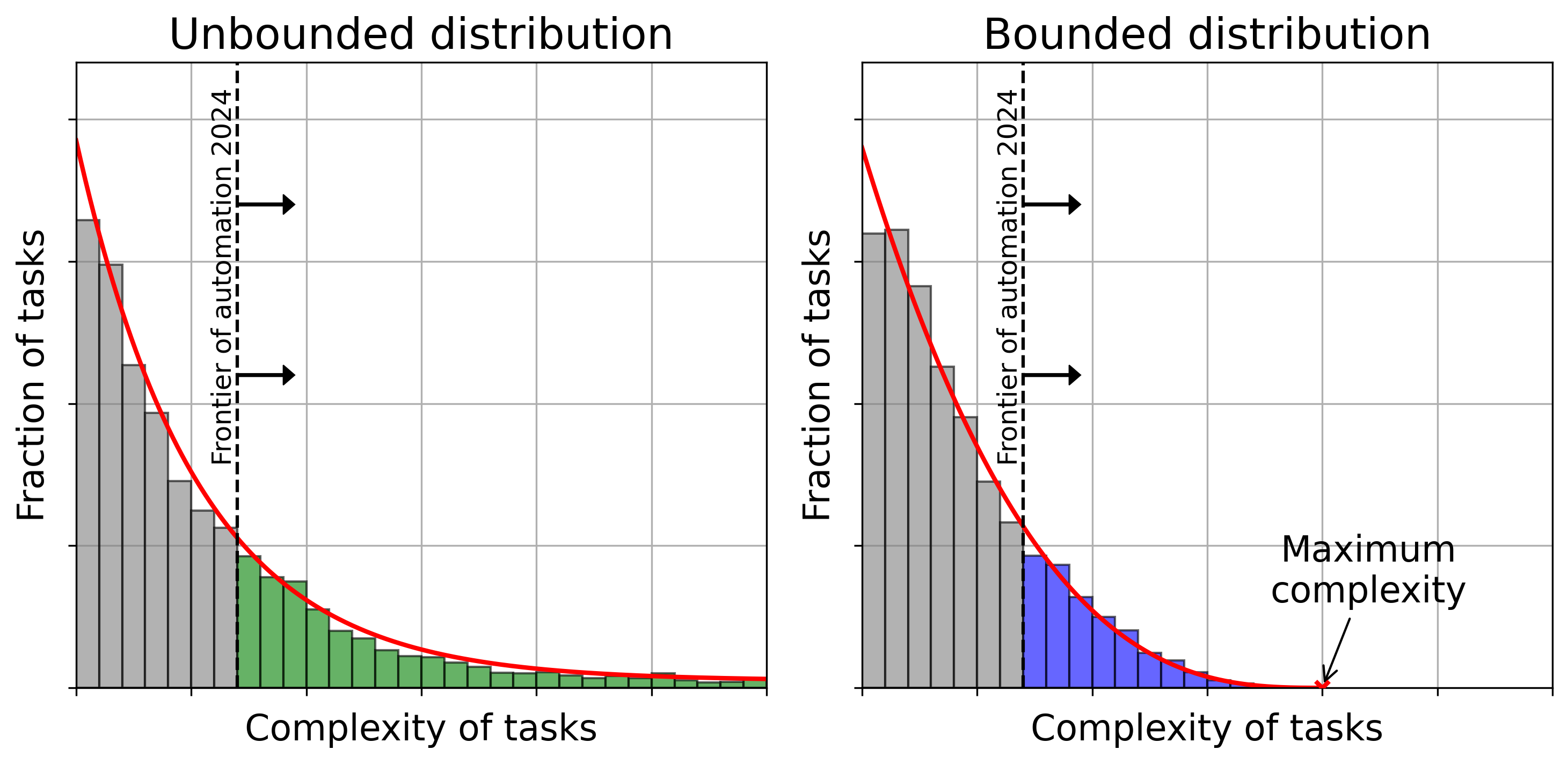
Figure 1: Unbounded and bounded distributions of tasks in complexity space

Throughout the paper, we analyze two opposing cases for the distribution of tasks in complexity space, which result in sharply different economic outcomes. First, we consider the possibility that human tasks are of unbounded complexity, illustrated in the left-hand panel of Figure 1. In this case, advances in the automation index, illustrated by the right-ward movement of the vertical “frontier of automation,” imply that more and more tasks are automated over time, but that there always remain tasks and by extension jobs that cannot be automated. Second, we consider a bounded distribution of task complexity, which reflects that the computational capabilities of the human brain are finite, as discussed, e.g., in Carlsmith, (2020). Bounded distributions result in full automation within finite time when the frontier of automation crosses the maximum complexity of tasks performed by humans. An alternative interpretation for tasks being to complex to automate is that society may choose not to automate certain tasks even when it is feasible to do so. This may apply, for example, to some of the tasks performed by priests, judges, or lawmakers.

We lay out an economic model in which atomistic tasks are gross complements that are combined to produce final goods. In the spirit of Zeira, (1998) and Acemoglu and Restrepo, (2018, 2022), all tasks can be performed by labor, and automated tasks can be performed by either labor or capital. However, unlike in the described works, our main focus is on the edge cases that arise as we come close to full automation.

Our analysis begins by examining the equilibrium under fixed supplies of capital and labor. We show that automation can have dramatic impacts on wages and output even before it reaches all tasks. There exists a threshold level of the automation index that separates two distinct regions. As long as the index remains below the threshold, labor remains scarce relative to capital, and wages remain high. However, once the automation index surpasses the threshold, the economy enters a second region, where the scarcity of labor is alleviated, despite the presence of some tasks that still need to be performed by humans. In this region, labor and capital become perfect substitutes at the margin so wages decline starkly to equal the marginal product of capital. The economy exhibits behavior akin to an $AK$ model.

Next, we characterize the effects of automation on the economy’s factor price frontier (FPF), which reflects all possible combinations of factor prices that may result from a given level of technology under different capital/labor ratios. The FPF provides general insights into the effects of automation that do not depend on specific assumptions on capital accumulation. We find that for a given level of automation, wages lie within a bounded interval that expands as the automation index rises – but only as long as automation is incomplete. Once all tasks are automated, the factor price frontier discontinuously collapses to a single point at which the effective returns to labor and capital are equalized. For given factor endowments, the effects of automation on wages are hump-shaped: for low levels of automation, advances in automation increase wages as the economy becomes more productive, but for higher levels of automation, wages decline due to the displacement of labor.

We analyze dynamic settings and show that the effects on wages are determined by a race between automation and capital accumulation. In addition to the previous two opposing effects on wages from rising productivity and labor displacement, automation also triggers capital accumulation that moves the economy up on the factor price frontier, increasing wages. We characterize an upper bound on output and wages that is reached in the limit case that the capital stock can instantaneously adjust to its optimal level whenever automation advances. We show a powerful analytic result: For any optimizing representative agent with linearly separable intertemporal preferences, the effects of automation on output and wages will lie between a lower bound captured by the constant-capital case and the described upper bound.

When the complexity distribution of tasks is bounded, full automation is reached in finite time and leads to a collapse in wages, no matter what savings behavior the representative agent pursues. For unbounded complexity distributions of tasks, we show that if the tail of remaining tasks is sufficiently thick, wages will rise forever. By contrast, if the tail of unautomated tasks is too thin, wages will eventually collapse.

Next, we simulate a range of scenarios to illustrate our findings numerically. (Figure 8 shows the main results.) We start with a “business-as-usual scenario,” which captures the traditional notion that a constant fraction of tasks is automated each period, similar to Aghion et al., (2019). This corresponds to a Pareto distribution for task complexity together with exponential growth in the automation index. Since the maximum complexity of tasks in this scenario is unbounded, true AGI will not be reached in finite time. In our calibration, both output and wages rise forever in this scenario, at a pace similar to what advanced countries have experienced over the past century.

Next we consider two AGI scenarios that span the range of estimates provided by Geoffrey Hinton, one of the godfathers of deep learning, who estimated in May 2023 that AGI may be reached within 5 to 20 years—after declaring that he had “suddenly switched [his] views on whether these things are going to be more intelligent than us.” In our “baseline AGI scenario” we assume a bounded task distribution such that full automation is obtained within 20 year. In an “aggressive AGI scenario” we assume a shorter-tailed distribution that implies full automation within five years. Our simulation results imply ten times faster growth than in the business-as-usual scenario, especially in the aggressive AGI scenario. However, wages collapse as the economy approaches full automation.

In a fourth scenario, we consider the possibility that there is a large bout of automation in the near term—for example because AI rapidly automates cognitive jobs—but that there remains a long tail of tasks that are harder to automate. As a result of the initial bout of automation, the economy enters the region in which labor loses its relative scarcity value, and wages in our simulation collapse. However, after capital accumulation has caught up sufficiently, labor becomes sufficiently scarce again so that the economy returns to region 1 and wages rise in line with output growth.

We extend our baseline model to analyze several additional important considerations. First, we consider the role of fixed factors (such as minerals or matter) and show that they may pose a bottleneck that holds back economic growth and worsens the outlook for wages, ultimately leading to stagnation accompanied by a wage collapse. Next, we add an innovation sector to analyze the potential for automating technological progress and show that this lifts the returns of all factors including wages. We illustrate that sufficient automation may give rise to a growth singularity whereby output takes off.

Furthermore, we analyze societal choices to retain certain jobs as exclusively human even when they can be automated (e.g., priests and judges), and show that a sufficient volume of such “nostalgic jobs” may help to keep labor sufficiently scarce so that wages continue to grow even when full automation is technically possible. We analyze the wage-maximizing rate of automation and show that slowing down automation in an AGI scenario may deliver significant gains to workers albeit at the cost of forgoing a growing fraction of output.

Next, we evaluate the impact of automation on workers with heterogeneous skills and susceptibility to being automated. We find that automation in such a scenario may give rise to an ever-declining fraction of superstar workers earnings ever-growing wages, whereas the majority of the labor force is starkly devalued by automation. Finally, we explore the role of compute as an example of specific capital that is tailored to automating specific tasks. We observe that in the short term, compute may earn very high returns, but after an adjustment period during which sufficient compute has been accumulated (and which may last long), compute may become just another form of capital that earns the same return as all other types of capital.

Related Literature

The foundational work of Aghion et al., (2019) explores the impact of artificial intelligence on economic growth, offering valuable insights into how technological advances in AI, including AGI, might influence future economic trajectories. Jones, (2023) underscores the risk of technological progress, emphasizing existential risk—a concept crucial in AGI discussions. Davidson, (2023) analyzes a model of the factors that may lead to a take-off in economic growth if technology advances near AGI but does not focus on the wage implications. Besiroglu et al., (2022) show how advances in AI may accelerate growth by speeding up R&D, and Erdil and Besiroglu, (2023) review the factors by which AGI may give rise to exponential growth. Trammell and Korinek, (2023) provide a useful survey on the broader implications of advanced artificial intelligence on economic growth.

A critical body of literature explores the dynamics between labor and automation. Seminal works by Acemoglu and Restrepo, (2018, 2022) and Autor, (2019) provide insights into how automation reshapes labor markets, focusing on technology as a substitute for individual worker tasks or how workers and tasks can complement or substitute for technology. Eloundou et al., (2023) and Felten et al., (2023) provide excellent empirical analyses of which tasks are amenable to automation by the current wave of foundation models. These studies offer a useful lens for understanding the economic implications of AI before AGI is reached. Our contribution to these strands of literature is to look at the limit case of what happens if either all work tasks are automated or we asymptote towards a world in which all tasks are automated.

Our paper is also related to a broader literature on AGI and superintelligence literature. Good, (1965) was the first to articulate the potential of an intelligence explosion if AGI is reached. Bostrom, (2014) provides a comprehensive exploration of superintelligence, highlighting the potential capabilities of AGI and the profound implications these might have for society. Yudkowsky, (2013) discusses several of the economic implications of the transition to AGI.

2 A Compute-Centric Model of Automation

2.1 Tasks in Compute Space

compute /km-pyüt/ verb: to determine by calculation         The system computed the length of the shortest path. noun: the combined computational resources available for information pro-          cessing tasks          Modern AI relies on vast amounts of compute. Etymology: Derived from the Latin verb "computare," meaning "to count, sum up, or reckon together," the word "compute" entered the English language as a verb in the 16th century. The noun form "compute" gained prominence more recently with the advent of high-performance digital computers and the increasing need to describe the resources required for computation.

Atomistic Job Tasks

A central assumption of our analysis is that the work performed by humans is composed of tasks and sub-tasks – or unchanging atomistic task – that differ in how easily they are automated. In our baseline model, we focus on cognitive tasks and their potential for automation. In this setting, an atomistic task is a well-defined computational assignment that contributes to the accomplishment of a larger job task.

These atomistic tasks are fundamental and are significantly smaller than the tasks that are listed in O*Net. Table 1 lists, for example, the top-5 O*Net tasks of economists: to study data; conduct and disseminate research; compile, analyze and report data; supervise research; and teach. Each of these O*Net “job tasks” involves a wide variety of different atomistic tasks. For example, the O*Net task “teach theories of economics” may require first planning the overall task, recalling different economic theories, synthesizing a structure, preparing slides, formulating lectures, synthesizing speech and affect, decoding and responding to student questions, preparing problem sets, distributing problem sets, grading problem sets, and so on—all while keeping track of the plan. It may also require tasks such as recognizing emotional expressions on students’ faces, using theory of mind to evaluate student progress and dynamically adjust the structure, etc.

All of these tasks involve a set of basic human brain functions, which constitute a form of computation. Some of these functions are easily performed by machines and therefore highly susceptible to cognitive automation (Korinek,, 2023), whereas others are more difficult. What matters for our purposes here is how computation-intensive they are using machines.

Recent literature on technology on labor markets observes that innovation typically gives rise to new job tasks (e.g., Acemoglu and Restrepo,, 2018; Autor,, 2019). This holds true when viewed from the perspective of high-level job tasks such as those captured by O*Net. However, when viewed from an atomistic level that reflects basic brain functions, innovation merely recombines atomistic tasks in novel ways to produce novel high-level tasks and jobs. For example, the novel task of “prompt engineering” may require atomistic tasks such as defining a desired output, crafting an initial prompt, entering it, reading the output, evaluating it, deciding whether to iterate, and finally sharing the output—all functions that existed long before the invention of generative AI systems that triggered prompt engineering.

• Study economic and statistical data in area of specialization, such as finance, labor, or agriculture.

• Conduct research on economic issues, and disseminate research findings through technical reports or scientific articles in journals.

• Compile, analyze, and report data to explain economic phenomena and forecast market trends, applying mathematical models and statistical techniques.

• Supervise research projects and students’ study projects.

• Teach theories, principles, and methods of economics.

Table 1: Top-5 Tasks performed by economists (O*Net database)

Task Complexity and Compute Intensity

Our baseline model emphasizes differences in complexity as a key dimension when studying the automation potential of tasks. Our preferred interpretation for what makes tasks difficult to automate is their compute intensity, which refers to the amount of computational resources required to perform a specific task. Compute intensity can easily be measured by the amount of floating point operations (FLOP) that need to be executed to perform a given task. The computational complexity for machines to execute a task often differs starkly from how easy or difficult it is for humans. Still, it is the computational complexity for machines that determines whether a task can be automated.

Advances in Computing

One of the main drivers of recent advances in AI has been the increased availability of computing power. Moore’s Law, first described by Gordon Moore, (1965), describes that the performance of cutting-edge computer chips doubles approximately every two years. The regularity has held for the past sixty years. Additionally, the amount of compute deployed in cutting-edge AI systems has grown even faster over the past decade, doubling roughly every six months, as shown in Sevilla et al., (2022) and depicted in Figure 2. Improvements in algorithms have further accelerated the growth in capabilities of cutting-edge AI systems (Besiroglu et al.,, 2022).

For our analysis below, we assume that there is an automation index that captures the maximum complexity of tasks that can be automated. This index grows exponentially at an exogenous rate, mirroring the type of advances captured by Moore’s Law and Figure 2. As the automation index increases, a growing mass of tasks can be automated.

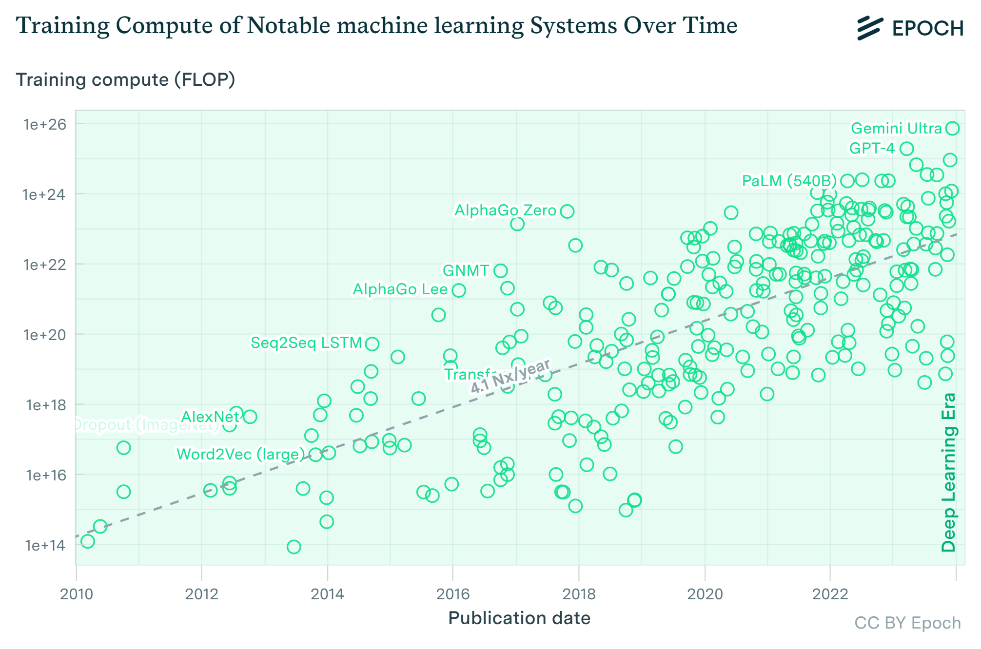
Figure 2: Training compute of frontier AI systems over time
(Copyright © 2024 by Epoch under a CC-BY-4.0 license; Sevilla et al.,, 2022.)

2.2 Baseline Model

Consider a representative household in a static economy who is endowed with $L=1$ units of labor and $K>0$ units of capital. There is a continuum of tasks that differ in their computational complexity $i$. The distribution function $\Phi(i)$ reflects the cumulative mass of tasks with complexity $\leq i$ and satisfies $\Phi(0)=0$ and $\lim_{i\rightarrow\infty}\Phi(i)=1$. If the distribution function is differentiable, we call its derivative $\phi(i)$ the density of tasks of complexity $i$. Examples are shown in Figure 1.

To produce aggregate output $Y$, we combine all the tasks of different complexity using a CES aggregator with elasticity of substitution $\sigma$.

$$Y=A\left[\int_{i}y(i){}^{\frac{\sigma-1}{\sigma}}d\Phi(i)\right]^{\frac{\sigma}{\sigma-1}}$$ (1)

where $y(i)$ is the amount of type $i$ tasks employed in the production of output. We generally assume $\sigma<1$, reflecting that the atomistic tasks are gross complements.

Each task is performed using capital $k(i)$ and labor $\ell(i)$ according to the production function

$$y(i)=a_{K}(i)k(i)+a_{L}(i)\ell(i)$$ (2)

where the coefficients $a_{K}(i)$ and $a_{L}(i)$ reflect the efficiency of capital and labor. We assume that the exogenous index $I$ reflects the state of automation and defines a complexity threshold such that all tasks below the threshold can be performed with either capital or labor but all the tasks above the threshold require labor. We normalize the technological parameters $a_{K}\left(i\right)=a_{L}\left(i\right)=1$ except that $a_{K}\left(i\right)=0$ if $i\geq I$. In other words,

$$y\left(i\right)=\begin{cases}k\left(i\right)+\ell\left(i\right)&\text{for }i<I\\ \ell\left(i\right)&\text{for }i\geq I\end{cases}$$

Strategies

The representative agent supplies her endowments of labor and capital every period at the prevailing factor prices $w$ and $R$ and makes no interesting economic decisions. The representative firm in the economy maximizes profits by hiring capital $k\left(i\right)$ and labor $\ell\left(i\right)$ for each task at the prevailing factor prices $w$ and $R$ to produce $y\left(i\right)$, which is then combined to produce final output. The firm’s maximization problem is

$$\max_{k(i),\ell(i)}Y-R\int_{i}k(i)d\Phi(i)-w\int_{i}\ell(i)d\Phi(i)\quad\text{s.t.}\quad(1),(2)$$

Equilibrium

An equilibrium in the baseline model consists of a set of $\left\{k\left(i\right),\ell\left(i\right),y\left(i\right)\right\}_{i\geq 0}$ and factor prices $w$ and $R$ such that the representative firm solves its maximization problem and markets for capital and labor clear, i.e.,

$$\int_{i}k(i)d\Phi(i)=K\qquad\int_{i}\ell(i)d\Phi(i)=1$$

Since there are no market imperfections, the described equilibrium also constitutes the first-best of the economy.

2.3 Equilibrium: Characterizing Two Regions

Scarcity of Labor

For given factor endowments $\left(K,L\right)$, there are two possible regimes for the scarcity of labor, depending on the level of the automation index $I$: If the index is low enough so that labor is relatively scarce, then the return on labor is greater than the return on capital, $w>R$, and the scarce labor is employed solely in those tasks that cannot be automated.

Conversely, if the state of automation is sufficiently advanced that only a small fraction of tasks are exclusive to human labor, then $w=R$ holds, and labor is employed not only in the remaining unautomated tasks but also in some of the automated tasks. At the margin, capital and labor are perfect substitutes.

Lemma 1 (Scarcity of labor).

For given $(K,L)$, there is a threshold value for the state of automation $\hat{I}$ that is defined by

$$\Phi\left(\hat{I}\right)=\frac{K/L}{1+K/L}$$ (3)

and increasing in the $K/L$-ratio such that there are two regions:

Region 1: If $I<\hat{I}$, then labor is scarce compared to capital. In this regime, labor is employed only for tasks with $i>I$. Output is

$$Y=F\left(K,L;I\right)=A\left[K^{\frac{\sigma-1}{\sigma}}\Phi(I)^{\frac{1}{\sigma}}+L{}^{\frac{\sigma-1}{\sigma}}(1-\Phi(I))^{\frac{1}{\sigma}}\right]^{\frac{\sigma}{\sigma-1}}$$ (4)

and wages satisfy

$$w=A^{\frac{\sigma-1}{\sigma}}\left(Y/L\right)^{\frac{1}{\sigma}}\cdot(1-\Phi(I))^{\frac{1}{\sigma}}>R$$

Region 2: If $I\geq\hat{I}$, then the relative scarcity of labor is relieved, and labor earns the same return as capital $w=R=A$; if the inequality is strict, some labor is deployed alongside capital for tasks with $i<I$, and labor and capital are perfect substitutes for the marginal task. Output is given by the linear function

$$Y=F\left(K,L\right)=A\left(K+L\right)$$ (5)

Conversely, for given $I$, there is a threshold $\kappa\left(I\right)=\Phi(I)/\left[1-\Phi\left(I\right)\right]$ such that the economy is in region 1 if $K/L>\kappa\left(I\right)$ and in region 2 if $K/L\leq\kappa(I)$. The threshold $\kappa(I)$ is increasing in $I$, i.e., if $K/L$ is marginally above the threshold, further automation pushes the economy from region 1 into region 2 where the scarcity of labor is relieved.

Proof.

Assume first that all labor is employed in tasks with $i\geq I$ and observe that the symmetry of the production function across all tasks implies that an identical amount of capital $k=K/\Phi(I)$ will be employed in each task below the threshold and an identical amount of labor $\ell=L/(1-\Phi(I))$ for each task above the threshold for given aggregate $K$ and $L$. The production function can then be written as

$$Y=F\left(K,L;I\right) =A\left[k^{\frac{\sigma-1}{\sigma}}\Phi(I)+\ell{}^{\frac{\sigma-1}{\sigma}}(1-\Phi(I))\right]^{\frac{\sigma}{\sigma-1}}$$

$$=A\left[K^{\frac{\sigma-1}{\sigma}}\Phi(I)^{\frac{1}{\sigma}}+L^{\frac{\sigma-1}{\sigma}}(1-\Phi(I))^{\frac{1}{\sigma}}\right]^{\frac{\sigma}{\sigma-1}}$$

proving equation (4).

The firm’s optimization problem implies the first-order conditions

$$F_{K} =A^{\frac{\sigma-1}{\sigma}}Y^{\frac{1}{\sigma}}\cdot K^{-\frac{1}{\sigma}}\Phi(I)^{\frac{1}{\sigma}}=R$$ (6)

$$F_{L} =A^{\frac{\sigma-1}{\sigma}}Y^{\frac{1}{\sigma}}\cdot L^{-\frac{1}{\sigma}}(1-\Phi(I))^{\frac{1}{\sigma}}=w$$ (7)

By comparing these two expressions, we can see that the return on capital $R$ is less than the return on labor $w$ as long as $K^{-\frac{1}{\sigma}}\Phi(I)^{\frac{1}{\sigma}}<L^{-\frac{1}{\sigma}}(1-\Phi(I))^{\frac{1}{\sigma}}$ or, equivalently, $k>\ell$, i.e., the capital assigned to each automated task is greater than the labor assigned to unautomated tasks. Expressing this in terms of aggregate supplies of factors, the condition is

$$\frac{K}{L}>\kappa(I):=\frac{\Phi(I)}{1-\Phi(I)}$$ (8)

The right-hand side is an increasing function of $I$ that goes from $0$ to $\infty$. By implication, there is a value of $I$ such that the inequality is violated for all $I>\hat{I}$.

When that threshold is crossed, it is more efficient to allocate some labor to tasks with $i<I$, and the marginal unit of labor is perfectly substituable with capital. By implication, $k\left(i\right)=\ell\left(i\right)=K+L$, and the CES aggregator simplifies to equation (5). Alternatively, the threshold for $\Phi(I)$ can be expressed explicitly as an increasing function of the $K/L$-ratio by solving for

$$\Phi\left(\hat{I}\right)=\frac{K/L}{1+K/L}$$

The remaining results stated in the lemma follow immediately. ∎

Intuitively, region 1 reflects the world as we have experienced it over the past 200 years, in which capital and labor are complementary in production, and labor is comparatively scarce. Figure 3 shows that for given factor supplies, a higher automation index $I$ increases the mass of tasks that can be accomplished with capital, implying that the available capital is spread over a greater number of tasks and becomes scarcer. Conversely, automation reduces the mass of tasks that is exclusive to labor, implying that the available labor can be concentrated on fewer tasks and becomes less scarce. As the automation index reaches the threshold $\hat{I}$, there are so few tasks left that are exclusive to labor that labor no longer enjoys a scarcity advantage over capital, and the returns on the two factors are equated.

Note that the threshold $\hat{I}$ depends solely on relative factor supplies, not on the elasticity of substitution $\sigma$ between capital and labor. As soon as labor is no longer scarce, it will be used interchangably with capital in the marginal task, and this holds even when individual tasks are highly complementary as reflected by low values of the elasticity of substitution (as long as $\sigma>0$).

Figure 3: Automation and the scarcity of labor

2.4 Factor Price Frontier (FPF)

For an analysis of the effects of advances in automation $I$ on factor returns, let us characterize the factor price frontier associated with the firm’s technology. The factor price frontier depicts all possible combinations of factor prices $R$ and $w$ that will result from different proportions of factor supplies $K$ and $L$ in a competitive economy with profit-maximizing firms under a given technology.

Lemma 2 (Factor Price Frontier (FPF)).

For a given automation index $I$, the factor price frontier slopes downwards, starting from a limiting point $w^{\ast}(I)=A(1-\Phi(I))^{\frac{1}{\sigma-1}}$ and $R=0$ as $K/L\rightarrow\infty$ to the point $w=R=A$ when $K/L\leq\kappa(I)$. Increases in $A$ move the FPF proportionately outwards. Increases in $I$ raise $w^{\ast}(I)$ and swivel the factor price frontier clock-wise.

Proof.

We obtain the factor price frontier from the aggregate cost function, which is the dual of the aggregate production function. The associated unit cost function represents the minimum cost at which a competitive optimizing firm can produce one unit of final output, given factor prices $w$ and $R$. In the region of $I<\hat{I}$, the unit cost function associated with equation (4) is

$$C(w,R;I)=\frac{1}{A}\bigg{(}R^{1-\sigma}\Phi(I)+w^{1-\sigma}(1-\Phi(I))\bigg{)}^{\frac{1}{1-\sigma}}$$

Since we employed the final good as the numeraire good, this cost function needs to equal 1 in a competitive economy. The factor price frontier when $I<\hat{I}$ is thus given by all pairs of $(w,R)$ that satisfy the equation $C\left(w,R;I\right)=1$, or equivalently,

$$w=\bigg{(}\frac{A^{1-\sigma}-R^{1-\sigma}\Phi(I)}{1-\Phi(I)}\bigg{)}^{\frac{1}{1-\sigma}}$$ (9)

Asymptotically, as $K/L$ goes to infinity, we can see from equations (6) and (7) that the return to capital $R$ goes to zero, whereas the wage converges to

$$w^{\ast}(I)=\lim_{K/L\rightarrow\infty}w=A\left[0\cdot\Phi(I)^{\frac{1}{\sigma}}+(1-\Phi(I))^{\frac{1}{\sigma}}\right]^{\frac{1}{\sigma-1}}(1-\Phi(I))^{\frac{1}{\sigma}}=A(1-\Phi(I))^{\frac{1}{\sigma-1}}$$ (10)

Conversely, when $I\geq\hat{I}$, the cost function is simply $C\left(w,R;I\right)=\min\left\{w,R\right\}/A$, and the factor price frontier is degenerate and consists of a single point $w=R=A$. ∎

Figure 4: Factor price frontier and its dependence on $A$

The factor price frontier is illustrated in Figure 4. The area above the 45 degree line corresponds to Region 1 of Lemma 1, reflecting a high capital-labor ratio $K/L>\kappa(I)$ and $w>R$. Higher capital intensity $K/L$ moves factor returns up and to the left along the frontier, i.e., it increases $w$ and reduce $R$. Conversely, when $K/L\leq\kappa(I)$, we enter Region 2 of the lemma, and the factor price frontier corresponds to a single dot on the 45 degree line at which $w=R=A$.

The right panel of Figure 4 shows how an increase in the level of technology $A$ pushes out the factor price frontier – for any ratio of $K/L$, it scales the returns of all factors proportionately. This exemplifies how the factor price frontier serves as a convenient tool to describe how factor returns are impacted by technological changes across any levels of factors supplies.

The Automation Path on the Factor Price Frontier

We next turn to the effects of automation for a given capital stock $K$ or equivalently, capital intensity $k=K/L$. Then it is easy to see that:

Lemma 3 (Automation and Output).

An increase in automation $d\Phi(I)$ raises output as long as $I<\hat{I}$, and leaves output unaffected otherwise.

Proof.

For $I<\hat{I}$, the result follows by differentiating expression (4),

$$\frac{dY}{d\Phi(I)}= \frac{1}{\sigma-1}A^{\frac{\sigma-1}{\sigma}}Y{}^{\frac{1}{\sigma}}\cdot\bigg{(}k^{\frac{\sigma-1}{\sigma}}-\ell^{\frac{\sigma-1}{\sigma}}\bigg{)}$$

Given $\sigma<1$, the derivative is positive as long as $k>\ell$, which is the condition for being in region 1 in Lemma 1 in which the production function is relevant. For $I\geq\hat{I}$, the relevant production function is (5), which is independent of $I$. ∎

Intuitively, for output to rise, capital must be sufficiently abundant, delivering a productivity gain from deploying the amply available capital to a greater number of tasks. This is frequently termed the productivity effect of automation.

Let us look at factor returns next.

Lemma 4 (Automation and Factor Returns).

(i) An increase in automation $d\Phi(I)$ always raises $R$ as long as $I<\hat{I}$. The effect on $w$ is hump-shaped: there is a threshold $I^{\ast}(K/L)$ with $\Phi(I^{\ast}(\cdot))\in(0,1)$ such that wages $w$ rise in $\Phi(I)$ as long as $I<I^{\ast}(K/L)$ or, equivalently, as long as $K/L>\kappa^{\ast}(I)$, but decline in $\Phi(I)$ for $I>I^{\ast}(K/L)$ or, equivalently, $K/L<\kappa^{\ast}(I)$.

(ii) For $\Phi(I)=0$, the return on capital is $R=0$, and wages equal $w=A$. For $\Phi(I)\geq\kappa/(1+\kappa)$, both equal $R=w=A$. The latter condition always holds if $\Phi(I)=1$.

Proof.

The limit results follow readily from equations (6) and (7) and from the second part of Lemma 1. By differentiating equation (6), with respect to $\Phi(I)$, we can see that automation always raises the return on capital.

To see how automation affects wages, consider the derivative of $\log w$ with respect to $\Phi$ from the firm’s optimality condition (7):

$$\frac{d\log w}{d\Phi(I)}= \frac{1}{\sigma-1}\frac{1}{\sigma}\bigg{(}k^{\frac{\sigma-1}{\sigma}}-\ell^{\frac{\sigma-1}{\sigma}}\bigg{)}(Y/A)^{\frac{1-\sigma}{\sigma}}-\frac{1}{\sigma}\frac{1}{1-\Phi(I)}.$$ (11)

The first term reflects the productivity effect of automation, which is positive under condition (8), reflecting that producing the marginal task using a relatively more abundant $k$ units of capital rather than a scarce $\ell$ units of labor increases output. The second term captures the displacement effect of automation and reduces labor income. It reflects that the labor used in each unautomated task $\ell=L/(1-\Phi)$ increases, as captured by the term in the denominator, thereby pulling down the marginal product of labor.

As $I$ rises, wages rise at first—at $\Phi(I)=0$ we find $\frac{d\log w}{d\Phi(I)}=\frac{1}{1-\sigma}>0$. As $I$ becomes larger, the first term in (4) declines, reaching zero for $I=\hat{I}$, and the absolute value of the second term grows and eventually dominates the first term—in the limit of $\Phi\rightarrow 1$, the second term becomes infinitely large. Thus, there exists an intermediate value $I^{\ast}(K/L)$ after which further automation reduces wages. Notice that the first term is increasing in $K/L$ whereas the second term is independent of $K/L$. The threshold can alternatively be expressed as $K/L<\kappa^{\ast}(I)$.

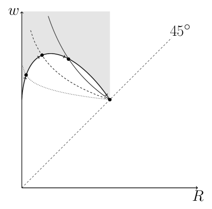
Figure 5: Factor price frontier and automation

∎

Figure 5 illustrates that an increase in automation $I$ “rotates” the factor price frontier clockwise, for example, from the dotted to the dashed and solid lines. If the economy is in the labor-scarce region 1 (above the 45 degree line), automation raises wages for a given return of capital and also the maximum wage level $w^{\ast}(I)$. For given $K/L$, the path of factor prices that results from rising automation $I$ is illustrated by the hump-shaped bold line with arrows in the figure. Along the path, $R$ rises continually whereas $w$ at first rises but eventually falls. When automation reaches $\hat{I}(K/L)$, the economy ends up in the degenerate equilibrium with $w=R=A$ on the 45-degree line.

2.5 Automation and Factor Earnings

Figure 6 shows the effects of automation on total output for given factor supplies as well as its split into the wage bill and the total returns to capital. The horizontal axis depicts the fraction $\Phi\left(I\right)$ of automated tasks, which goes from zero to one. The left-hand panel illustrates the case of equal capital and labor endowments, $K=L=1$, and modest complementarity with an elasticity of substitution $\sigma=0.5$ between the two. As long as the economy is in the scarce-labor region (Region 1), output is a strictly monotonic function of automation. At first, automation almost exclusively benefits labor, and the returns to capital are minuscule. But as automation increases and we come closer to Region 2, the wage bill reaches a ceiling and starts to decline. Further automation still raises output, but the returns to capital grow faster than output, at the expense of the wage bill. When Region 2 is reached at $\Phi=0.5$, both factors earn equal returns. Given equal endowments, this translates into capital and labor shares of one-half each.

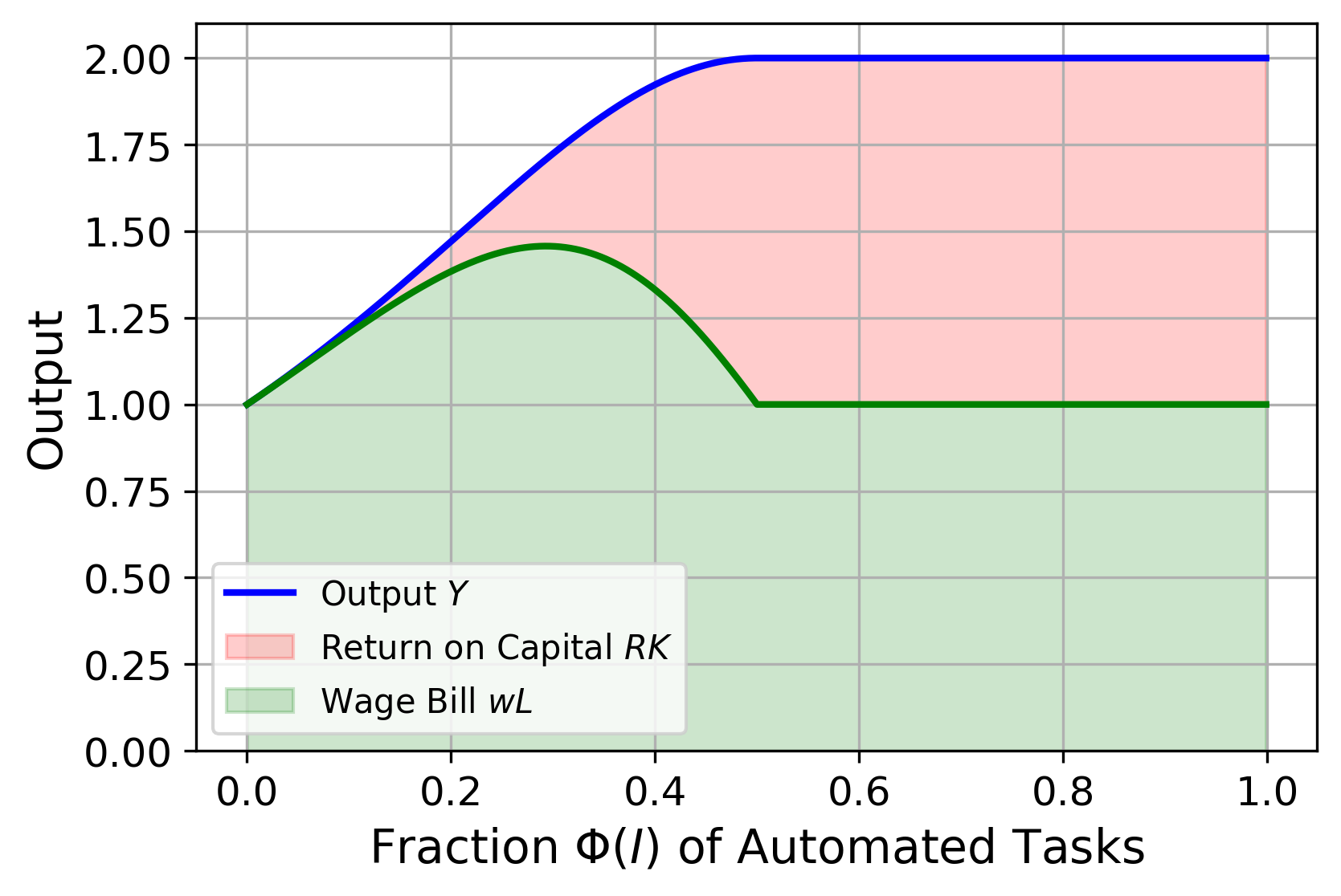
(a) Equal factor endowments

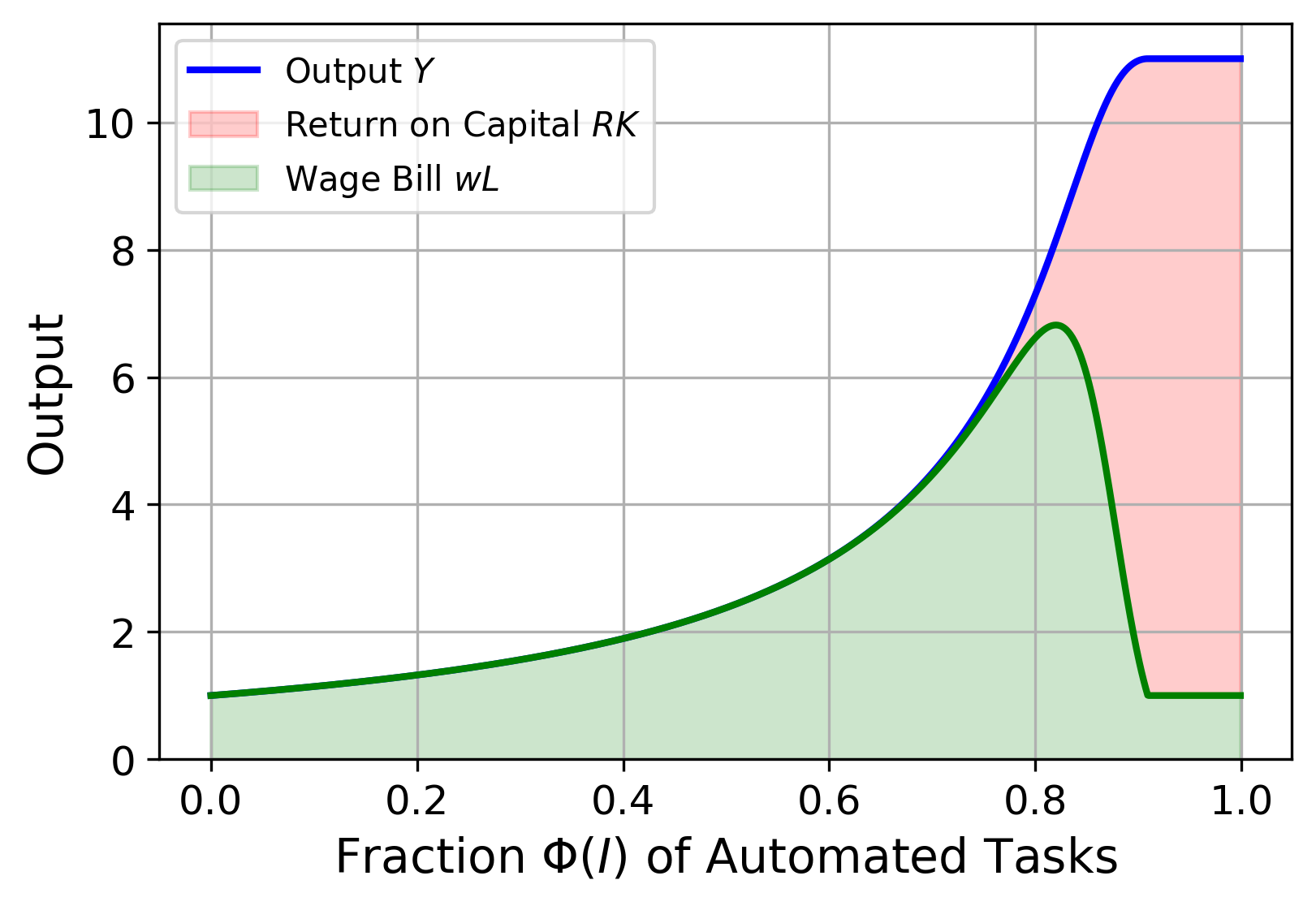
(b) Abundant effective capital

Figure 6: Static equilibria under rising automation

The right panel of the figure shows an alternative scenario in which the effective supply of capital is ten times higher than labor, i.e., $L=1$ and $K=10$, and in which the two are strong complements with $\sigma=0.2$. The abundance of capital and the strong complementarity imply that the region in which most of the benefits go to labor is much larger, but so is the drop in the wage bill once a critical threshold is surpassed: whereas wages seem to be growing exponentially in $\Phi\left(I\right)$ up until $\Phi\approx 0.80$, they experience a precipitous decline by about 85% starting around $\Phi\approx 0.83$, accompanied by a meteoric rise in the returns to capital. When Region 2 is reached at $\Phi=10/11$, factor returns are equalized, and given the relative factor endowments, the capital share of the economy is ten times the labor share. This example highlights that the fate of labor can change rapidly when certain thresholds are crossed.

Crucially, the effect of automation on output—and per-capita income—depends on the capital available. In the illustration in the left panel, full automation merely doubles output; in the right panel, output grows eleven-fold. This observation naturally leads us to the next step of our analysis—to analyze how automation interacts with capital accumulation in a dynamic setting.

3 Dynamics: The Race between Automation and Capital Accumulation

The dynamics of output and wages depend not only on technological advances—captured by the automation index $I$—but also on capital accumulation and by extension on the savings behavior of the agents in the economy. This section analyzes these forces in a dynamic setting.

3.1 Automation Scenarios

Progress in automation

We assume that the automation index $I$ grows exponentially over time at an exogenous rate of $g$, reflecting Moore’s law and similar regularities. For an initial $I_{0}$, the time path of $I$ (omitting the time index $t$ for conciseness) is given by

$$I=I_{0}e^{gt}$$

We can equivalently write that $\log I=\log I_{0}+gt$ grows linearly at the rate $g$.

We consider different distributions $\Phi\left(i\right)$ of task complexity or tasks in compute space to capture alternative scenarios for the advent of AGI:

Business-As-Usual Scenario (Unbounded Distribution)

We model unbounded complexity distributions of tasks $\Phi\left(i\right)$ as Pareto, implying that $\log i$ is described by an exponential distribution, $\log i\sim Exp(\lambda)$ with decay parameter $\lambda$. The resulting cumulative distribution function is $\Phi(i)=1-e^{-\lambda\log i}$. If the automation index $I$ grows exponentially at rate $g$, the fraction of non-automated tasks declines at rate $\lambda\cdot g$. This distribution has an infinite right tail, meaning that there will always be tasks that cannot be automated.

Baseline and Aggressive AGI Scenarios (Bounded Distributions)

For our AGI scenarios, we assume a bounded complexity distribution of tasks to capture the scenario that the tasks that can be performed by human brains is limited by an upper bound so automation crosses the threshold $\hat{I}$ within finite time. We assume that $\Phi(i)$ follows a power function $\Phi(i)=1-(1-\log i/\log I^{\max})^{\beta}$ with $\beta=1$ and with normalization $I^{\max}=I_{0}e^{gT}$ such that all tasks are automated after $T$ years. Following Hinton’s predictions, we set $T=20$ in the baseline AGI scenario and $T=5$ in the aggressive AGI scenario. For $I>I^{\max}$, we keep $\Phi(i)=1$ capturing full automation.

Bout of Automation (Mixed Distribution)

We consider a fourth scenario in which rapid advances in AI automate a large fraction of tasks within a short time span, but in which we assume that there remains an unbounded tail of tasks that cannot be automated, for example, because of legal or cultural reasons. Analytically, we assume a mixture of the two scenarios above. Specifically, $\Phi(i)$ is defined as $\Phi(i)=\omega\bigg{[}1-\left(1-\log i/\log I^{\max}\right)^{\beta}\bigg{]}+(1-\omega)\bigg{[}1-e^{-\lambda\log i}\bigg{]}$ where $\omega\in[0,1]$ is a weight parameter. We assume the same values for the parameters of the Pareto and power function distributions as in the previous two cases.

3.2 Consumer Problem

The representative household seeks to maximize its lifetime utility by choosing consumption $C_{t}$ over time:

$$\max_{\{C_{t}\}}U=\int_{0}^{\infty}e^{-\rho t}u(C_{t})dt$$ (12)

subject to the law of motion for capital:

$$\dot{K}_{t}=F(K_{t},L_{t};I_{t})-\delta K_{t}-C_{t}$$ (13)

for given $K_{0}$. The current-value Hamiltonian for this problem is:

$$H_{c}=u(C_{t})+\mu_{t}\left[F(K_{t},L_{t})-\delta K_{t}-C_{t}\right]$$

The first-order conditions with respect to consumption and capital are:

$$\frac{\partial H_{c}}{\partial C_{t}} =u^{\prime}(C_{t})-\mu_{t}=0$$

$$\frac{\partial H_{c}}{\partial K_{t}} =\mu_{t}\left[F_{K}-\delta\right]=-\dot{\mu}_{t}+\rho\mu_{t}$$

Differentiating the first optimality condition with respect to time yields $u^{\prime\prime}(C_{t})\dot{C}_{t}=\dot{\mu}_{t}$, and substituting into the second optimality condition gives

$$\frac{\dot{C}_{t}}{C_{t}}=\frac{1}{\eta(C_{t})}\left[F_{K}(K_{t},L_{t})-\rho-\delta\right]$$ (14)

where $\eta(C_{t})=-\frac{u^{\prime\prime}(C_{t})C_{t}}{u^{\prime}(C_{t})}$ is the elasticity of intertemporal substitution.

Limit Behavior in Region 2

When the economy is in region 2, then $F_{K}=A$. If the agent’s utility function exhibits constant elasticity of substitution $\eta$, then the Euler equation implies a constant growth rate of consumption

$$g_{C}=\frac{\dot{C_{t}}}{C_{t}}=\frac{A-\rho-\delta}{\eta}$$ (15)

Let us assume that $A>\rho+\delta$ so consumption growth is positive and consider the case that the economy remains in region 2 forever—for example, because full automation $\Phi(I)=1$ has been reached. Then the economy will converge towards a balanced growth path in which $g_{Y}=g_{K}=g_{C}$ as in (15) and the savings rate $s^{\infty}=1-C/Y$ is constant. From (13), we obtain that

$$g_{K}=\frac{\dot{K_{t}}}{K_{t}}=\frac{sA(K_{t}+L)}{K_{t}}-\delta$$

As $\lim_{t\rightarrow\infty}L/K_{t}=0$, we can equate $g_{C}=g_{K}$ and solve for the long-run savings rate

$$s^{\infty}=\frac{A-\rho-\delta+\eta\delta}{A\eta}=\frac{1}{\eta}-\frac{\rho+(1-\eta)\delta}{A\eta}$$

Bounds

Assume an initial $I_{0}$ and $K_{0}$ that satisfy $F_{K}\left(K_{0},L;I_{0}\right)\geq\rho+\delta$, i.e., there was no excessive capital accumulation in the past. Then the following proposition holds for any intertemporal utility function that is linearly separable as specified in (12) with a twice continuously differentiable, increasing, and strictly concave period utility function $u(C)$:

Proposition 5 (Bounds for Output and Wages).

For any distribution $\Phi\left(i\right)$ of tasks in compute space and exogenous growth in the automation index $I_{t}$, the paths of capital, output, and wages lie between lower and upper bounds $K^{-}\leq K_{t}\leq K_{t}^{+}$, $Y_{t}^{-}\leq Y_{t}\leq Y_{t}^{+}$ and $w_{t}^{-}\leq w_{t}\leq w_{t}^{+}$.

The lower bounds are defined by the fixed-capital case with $K^{-}=K_{0}$ $\forall t$ and $Y_{t}^{-}=F(K^{-},L,I_{t})$, $w_{t}^{-}=F_{L}(K^{-},L,I_{t})$. The lower bound on wages first rises in $I_{t}$ and then declines in $I_{t}$. It declines to $A$ in finite time if full automation is reached asymptotically, i.e., if $\lim_{I\rightarrow\infty}\Phi(I)=1$.

If $\Phi(I_{t})<1$, an upper bound $K_{t}^{+}$ for capital is defined by $F_{K}\left(K_{t}^{+},L,I_{t}\right)=R=\rho+\delta$ $\forall t$ as long as a solution exists; otherwise we set $K_{t}^{+}=\infty$. The upper bounds for output and wages are $Y_{t}^{+}=F(K_{t}^{+},L,I_{t})$ and $w_{t}^{+}=F_{L}(K_{t}^{+},L,I_{t})$. All three upper bounds are increasing in the automation index $I_{t}$. If automation is full, $\Phi(I_{t})=1$, the upper bounds are $K_{t}^{+}=\infty$ and $Y_{t}^{+}=\infty$, and the upper bound on wages discontinuously collapses to $w_{t}^{+}=A$.

Proof.

Observe that for any twice continuously differentiable period utility function that is increasing and strictly concave, the elasticity in the Euler equation (14) satisfies $\eta(C_{t})\in(0,\infty)$. Consumption on the optimal path is increasing as long as $F_{K}>\rho+\delta$ and constant when $F_{K}=\rho+\delta$. Our characterization of the factor price frontier delivers most of the remaining results.

For the lower bound, observe that increases in $I$ and $\Phi(I)$ raise the marginal product $F_{K}$ for given $K$, triggering additional capital accumulation, which raises output and wages above the lower bound. For the upper bound, observe that by the Euler equation, capital accumulation will never exceed the upper threshold $K_{t}^{+}$, which is given by

$$K_{t}^{+}=\frac{A^{\sigma}L(1-\Phi(I_{t}))^{\frac{1}{\sigma-1}}\Phi(I_{t})}{(R^{\sigma-1}-A^{\sigma-1}\Phi(I_{t}))^{\frac{\sigma}{\sigma-1}}}.$$ (16)

For given $I_{t}$, output and wages are increasing in $K_{t}$, implying that they must lie between the lower and upper bounds defined by $K^{-}$ and $K_{t}^{+}$. If $\Phi(I_{t})=1$, the production function is $AK$-style, and Lemma 4 implies that $w_{t}=A$. ∎

On the factor price frontier, the lower bound on wages $w^{-}$ is pinned down by the automation path in Figure 5; it collapses to $A$ in finite time if the economy asymptotically converges to full automation. As long as $\Phi(I)<1$, the upper bound on wages $w_{t}^{+}$ is pinned down by the intersection of the corresponding factor price frontier with a vertical line at $R=\rho+\delta$ and rises without bounds in $I$. However, when full automation $\Phi(I)=1$ is reached, the upper bound on wages $w_{t}^{+}$ discontinuously collapses to $A$, which equals the lower bound and must therefore equal the equilibrium wage. This result is independent of intertemporal preferences and savings behavior and occurs in finite time if the distribution of task complexity $\Phi(I)$ is bounded, as in our two AGI scenarios.

The Balancing Savings Rate

To further investigate the race between automation and capital accumulation, we analyze the threshold at which the wage effects of automation and capital accumulation precisely offset each other. For this, we take the total differential of the equilibrium wage, $w_{t}=F_{L}(K_{t},L;I_{t})$, and set $dw_{t}=0$ to find

$$F_{KL}(K_{t},L;I_{t})\frac{dK_{t}}{dt}+F_{LI}(K_{t},L;I_{t})\frac{dI_{t}}{dt}=0$$ (17)

Suppose, for simplicity, that $\delta=0$ so we can denote the savings rate at $t$ by $s_{t}=\dot{K}_{t}/Y_{t}$. Also, note that $F_{LI}(K_{t},L;I_{t})\frac{dI_{t}}{dt}=F_{L\Phi}\dot{\Phi}_{t}$. Then

$$s_{t}Y_{t}\cdot F_{KL}=-F_{L\Phi}\dot{\Phi}_{t}$$

The left-hand side is the increase in wages due to capital accumulation. The right-hand side is the change in wages due to automation. As we observed above in Lemma 4, the term $F_{L\Phi}$ encompasses the productivity effect and the displacement effect of automation on wages. Dividing by the cross-derivative $F_{KL}$, the fraction $\frac{F_{L\Phi}}{F_{KL}}$ captures the wage effects of automation relative to capital accumulation. After some algebra, we obtain

$$\frac{F_{L\Phi}}{F_{KL}}=\bigg{[}\frac{\sigma}{1-\sigma}(k/\ell)^{\frac{1-\sigma}{\sigma}}-\bigg{(}\kappa+\frac{1}{1-\sigma}\bigg{)}\bigg{]}k$$

The first term in the brackets is the productivity effect that is increasing in the relative abundance of capital $k/\ell$ – if capital is very abundant compared to labor, then using capital for newly automated tasks significantly raises output. The second term is the displacement effect that is increasing in $\kappa$ and thus in the automation index $I$. (Recall that for the given level of automation $I,$ $\kappa\left(I\right)=\Phi(I)/\left[1-\Phi\left(I\right)\right]$ reflects the threshold of the capital/labor ratio below which the economy is in region 2 such that the scarcity of labor is lifted.) Intuitively, if a large fraction of tasks has already been automated, then further automation of marginal tasks will result in a large fall in labor demand since the automated labor has to be reallocated to an ever smaller set of human-only tasks.

By rearranging terms, we obtain the following expression for the savings rate that, given $\Phi$ and $g$, perfectly offsets the effect of automation on wages

$$\tilde{s}_{t}=\bigg{[}\bigg{(}\kappa+\frac{1}{1-\sigma}\bigg{)}-\frac{\sigma}{1-\sigma}(k/\ell)^{\frac{1-\sigma}{\sigma}}\bigg{]}\cdot\frac{K_{t}}{Y_{t}}\cdot\frac{\phi_{t}I_{t}}{\Phi_{t}}\cdot g$$ (18)

The condition tells us that, to offset the effect of automation on wages, the savings rate must be increasing with (i) the displacement effect net of the productivity effect, (ii) the capital-output ratio, (iii) the relative mass of automated tasks at the current compute threshold for task automation, and (iv) the growth of compute $g$. Intuitively, a large fraction of output must be invested if (i) the displacement effect reduces wages significantly, or (ii) there is already a large amount of capital stock in the economy, or (iii) a large amount of tasks are being automated, or (iv) automation is fast.

The expression in (18) tells us about the threshold level for the savings rate at time $t$ above which wages rise and below which wages fall, given the extent of automation occurring at time $t$. In other words, it characterizes the short-run behavior of wages as an outcome of the race between automation and capital accumulation.

Long-Run Dynamics for Unbounded Task Distributions

To further illuminate the trade-off in (18), we turn to the long-run dynamics of wages. To do so, we start by characterizing the conditions for the existence of a balanced growth path (BGP). We define a BPG as an equilibrium path on which output and capital stock grow at a constant rate and factor shares remain constant.

Lemma 6.

Suppose that as $t$ increases, $\Phi(I_{t})\rightarrow 1$, and focus on the limit case. Then the return to capital converges to $A$. Moreover, output and capital stock grow at the rate $(A-\rho-\delta)/\eta$ and the savings rate converges to $(A-\rho-\delta+\eta\delta)/A\eta$.

Proof.

If the economy is in region 1 in the limit, then the production function converges to

$$\lim_{\Phi\rightarrow 1}A\left[K^{\frac{\sigma-1}{\sigma}}\Phi{}^{\frac{1}{\sigma}}+L^{\frac{\sigma-1}{\sigma}}(1-\Phi)^{\frac{1}{\sigma}}\right]^{\frac{\sigma}{\sigma-1}}=AK$$

If the economy is in region 2 in the limit, then $F(K,L)=A(K+L)$. In both cases,

$$\lim_{\Phi\rightarrow 1}F_{K}=A$$

As a result, the Euler equation implies

$$\frac{\dot{C}_{t}}{C_{t}}=\frac{1}{\eta}[F_{K}-\rho-\delta]\rightarrow\frac{1}{\eta}[A-\rho-\delta]$$

as $\Phi\rightarrow 1$. Output and capital must grow at the same rate, which implies that the savings rate must satisfy

$$\frac{\dot{C}_{t}}{C_{t}}=\frac{\dot{K}_{t}}{K_{t}}=\frac{s^{\infty}Y_{t}}{K_{t}}-\delta$$

Since $\lim_{\Phi\rightarrow 1}\frac{Y_{t}}{K_{t}}=A$, this requires that $\dot{K}_{t}/K_{t}\rightarrow s^{\infty}A-\delta$. Therefore, we have

$$s^{\infty}A-\delta =\frac{1}{\eta}[A-\rho-\delta]$$

$$s^{\infty} =\frac{A-\rho-\delta+\eta\delta}{A\eta}$$

∎

Since we are interested in the long-run dynamics of wages, we make a simplifying assumption that the savings rate is given exogenously at a constant value $s^{\infty}$, which can be interpreted as the long-run savings rate. Under the assumption, $s$ is a key parameter determining the rate of capital accumulation. Depending on the value of $s^{\infty}$ relative to the rate of automation $g$, the race between automation and capital accumlulation can result in three possible outcomes. The following proposition summarizes the results.

Figure 7: Wage growth rate ($g_{w}$) as a function of the rate of automation ($\lambda g$)

Proposition 7 (Race between automation and capital accumulation).

Suppose the complexity distribution of tasks is Pareto and that the economy starts in region 1, i.e., $I_{0}<\hat{I}_{0}$. Then the growth of wages and long-run labor shares are characterized by two thresholds on the rate of automation $\lambda g$:

1. If $\lambda g>\frac{A-\rho-\delta}{\eta}$ then $\lim_{t\rightarrow\infty}w_{t}=A$ and the labor share converges to zero.

2. If $\frac{A-\rho-\delta}{\eta}\cdot(1-\sigma)<\lambda g\leq\frac{A-\rho-\delta}{\eta}$ then wages grow exponentially at an asymptotic rate $\frac{1}{\sigma}\bigg{(}\frac{A-\rho-\delta}{\eta}-\lambda g\bigg{)}$ and the labor share converges to one.

3. Lastly, if $\lambda g\leq\frac{A-\rho-\delta}{\eta}\cdot(1-\sigma)$ then wages grow exponentially at an asymptotic rate $\frac{\lambda g}{1-\sigma}$ and the labor share converges to $1-\bigg{[}\frac{(A-\rho-\delta+\eta\delta)/\eta}{\frac{\lambda g}{1-\sigma}+\delta}\bigg{]}^{\frac{\sigma-1}{\sigma}}$.

Proof.

See Appendix A.1. ∎

Intuitively, the proposition illustrates how wages evolve as the result of a race between automation and capital accumulation. As observed above, the fraction $\frac{A-\rho-\delta}{\eta}$ is proportional to the long-run savings rate of the economy. In the first case, if the rate of task automation $\lambda g$ is too high compared the savings rate, then the automation index $I$ crosses the threshold $\hat{I}$ in finite time and the economy transitions into region 2, where wages collapse to $A$ and remain stagnant. If the rate of task automation $\lambda g$ is at an intermediate value, then wage growth is constrained by capital accumulation. Wages grow perpetually at rate $\frac{1}{\sigma}(\frac{A-\rho-\delta}{\eta}-\lambda g)$, which is proportional to the savings rate minus the rate of automation. Finally, if $\lambda g$ is low enough, then the rate of automation rather than capital accumulation constrains wage growth. In other words, wage growth depends on how fast automation increases the efficiency of factor allocation and allows the utilization of abundant capital. Indeed, the growth rate of wages (and of the entire economy) in this regime is increasing in the rate of automation.

Figure 7 illustrates the three cases in Proposition 7. The figure plots the long-run growth rate of wages as a function of the rate of automation. If $\lambda g$ is sufficiently low as in case 1, then the wage growth rate is increasing in the rate of automation as the upward-sloping part of the curve indicates. Once $\lambda g$ surpasses the first threshold value, the growth rate of wages starts to decline as $\lambda g$ increases further. Lastly, if $\lambda g$ surpasses the second threshold value, then wages do not grow in the long run and stay at $A$.

3.3 Numerical Illustration

Parameter	Value	Description
$\rho$	0.04	Discount rate
$\eta$	2	Risk aversion parameter
$\delta$	0.1	Depreciation rate
$\sigma$	0.5	Elasticity of substitution
$A$	0.5	Total factor productivity
$L$	1	Labor endowment
$\Phi_{0}$	0.608	Initial fraction of automated tasks
$K_{0}$	4.6	Initial capital stock

Table 2: Parameter values for the numerical illustration

To provide an illustration of the theoretical results, we present simulations of the four automation scenarios described in Section 3.1. Table 2 summarizes the parameter values that were common to all the simulations. The first five parameters are standard in the literature, and $L=1$ is a normalization. We chose $\Phi_{0}$ and $K_{0}$ to match a 66% initial labor share with capital at its steady state for that level of technology.

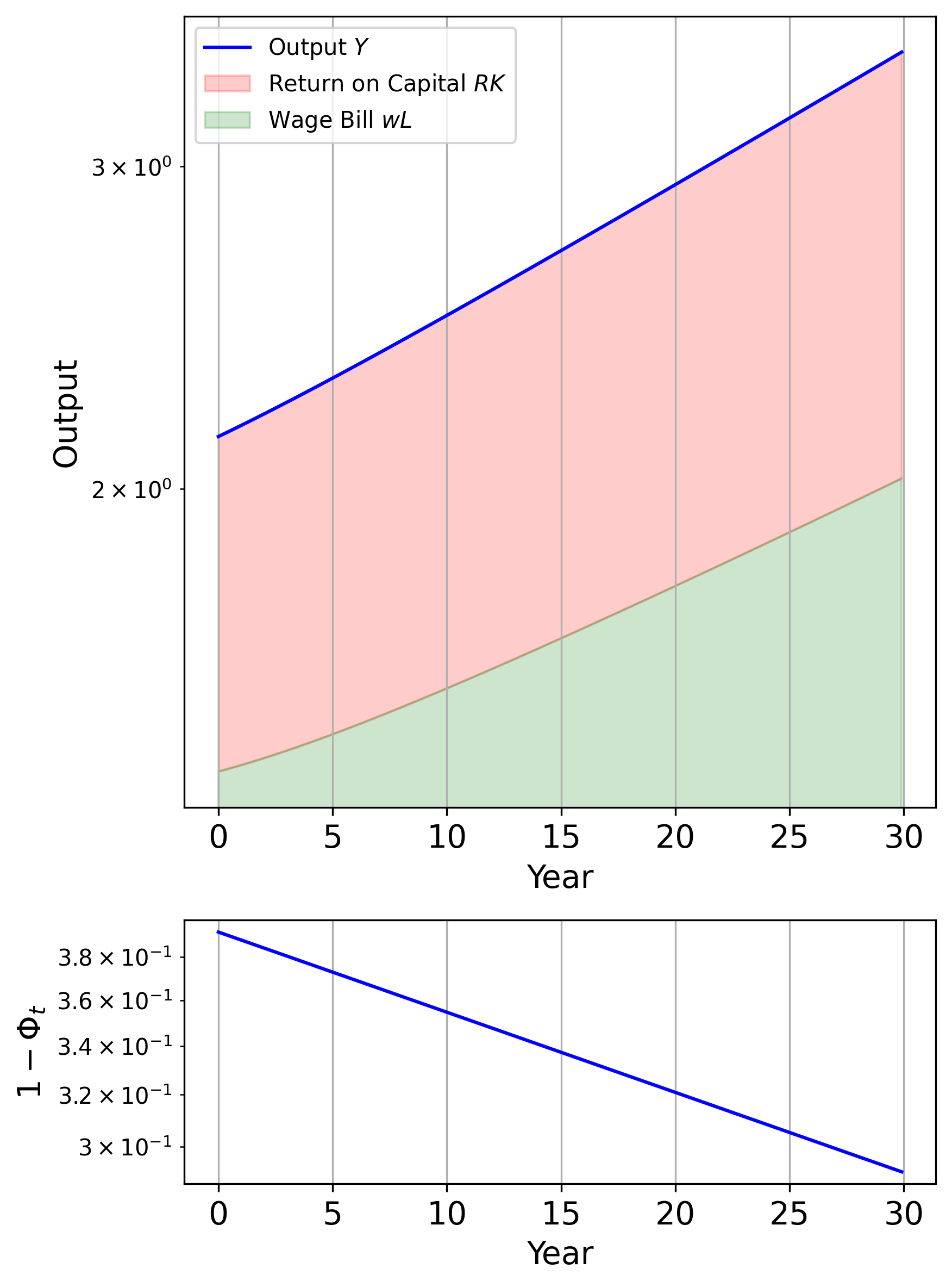
(a) Business-as-usual scenario

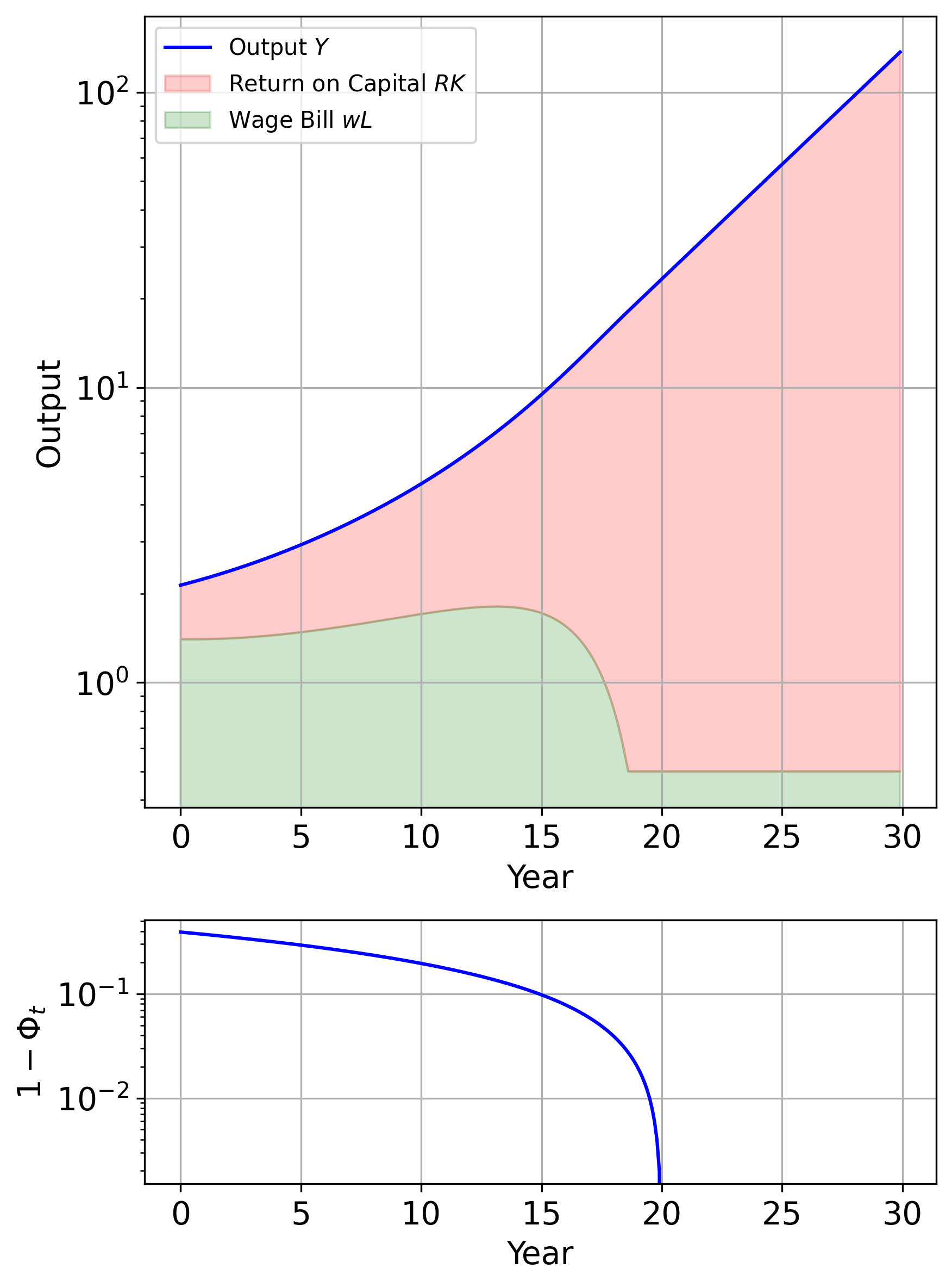
(b) Baseline AGI scenario

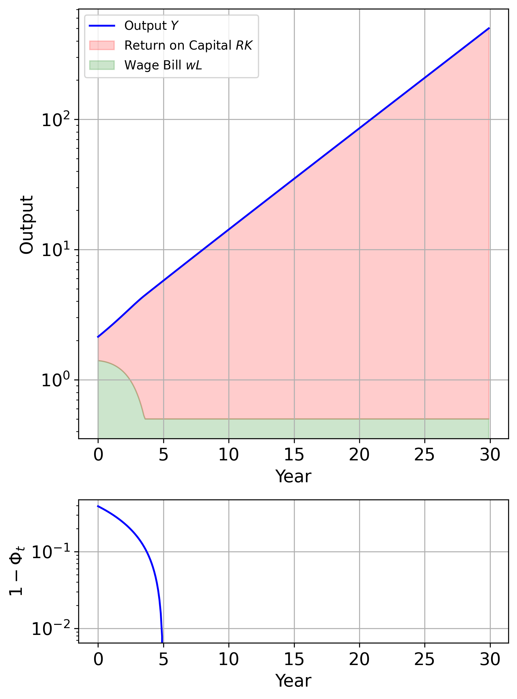
(c) Aggressive AGI scenario

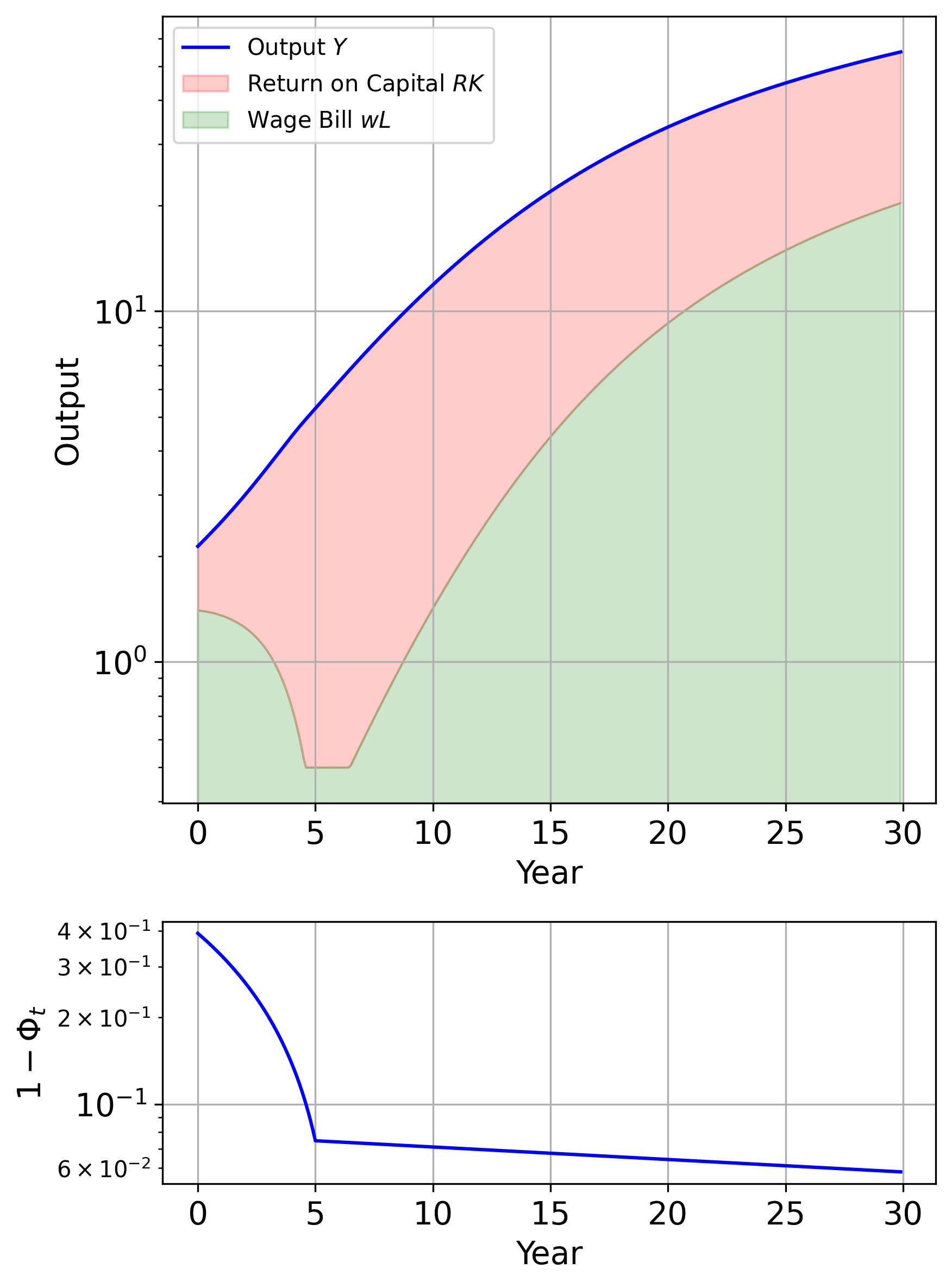
(d) Mixed scenario

Figure 8: Simulations of the four scenarios

Figure 8 presents the results. Panel (a) shows the traditional automation scenario “business-as-usual,” in which $\Phi(i)$ reflects a rate of task automation of $\lambda g=0.01$ per year. The upper part of the panel shows the output, split into the returns to capital (red, upper area) and the wage bill (green, lower area), on a logarithmic scale. The lower part of the panel shows the fraction of unautomated tasks $1-\Phi$ on a logarithmic scale—for panel (a), this is a straight line, capturing exponential decay. We observe that in the “business-as-usual” scenario, output grows at approximately 2% per year, and both the returns to capital and the wage bill rise approximately in tandem (with a small decline in the labor share due to the effects of automation). Note that this scenario corresponds to case 3 in Proposition 7, i.e., capital accumulation is sufficiently fast so that growth is constrained by the speed of automation.

Panels (b) and (c) show the AGI scenarios, in which the fraction of unautomated tasks collapses to zero in 20 or 5 years, respectively. In the baseline AGI scenario, wages grow slightly during the initial periods but then collapse before full automation is reached. After the collapse, wages are equal to the returns to capital, and the economy remains in region 2 where labor and capital are perfectly substitutable, with steady-state growth of 18% per year. In the aggressive AGI scenario, the wage collapse happens after about 3 years. Since the scarcity of labor is relieved earlier than in the baseline AGI scenario, the growth take-off occurs earlier.

Panel (d) shows the “bout-of-automation” scenario. During the initial periods, a large fraction of tasks are automated, leading to wage collapse similar to the aggressive AGI scenario as the economy enters region 2—labor is abundant because of the rapid automation and comparatively low capital stock. However, over time, the economy accumulates more capital, making labor scarcer again. Around year 9, the economy has accumulated sufficient capital so that it returns to region 1. Wages rise above $A$ and start growing again in line with further (slower) advances in automation and further capital accumulation. This scenario illustrates the possibility that labor demand may collapse due to rapid automation but recover later because of a long tail of tasks that cannot be automated.

4 Extensions

4.1 Fixed Factors and the Return of Scarcity

If labor is dethroned as the most important factor of production, it becomes useful to disentangle the remaining factors, which have traditionally been lumped together into “capital” in the economic models of the Industrial Age. Let us distinguish between factors that are in fixed supply and factors that are reproducible and can therefore be accumulated. We continue to call all reproducible factors “capital,” including compute, robots, power plants, and factories. By contrast, factors in fixed supply include land, space, minerals, or solar radiation. It is difficult to predict which scarce factors will matter the most in an AGI-powered future – in the short term, it is likely that microchips and the semiconductor fabrication equipment (“fabs”) used for producing these chips will be bottlenecks, but these are clearly reproducible. By contrast, the raw materials going into the production of chips, for example certain rare earth minerals, are irreproducible. In the longer-term, matter or, equivalently, energy ($E=mc^{2}$) may be the ultimately source of scarcity.

For the purposes of our analysis, we incorporate a fixed factor in our analysis that we label $M$ for minerals or matter. We assume that the aggregate production function is a Cobb-Douglas aggregator of the task composite and $M$,

$$Y=A\left[\int_{i}y(i){}^{\frac{\sigma-1}{\sigma}}d\Phi(i)\right]^{\frac{\sigma}{\sigma-1}\cdot\alpha}M^{1-\alpha}$$ (19)

where $\alpha\in[0,1]$ is the share of the composite among total output. Then, a version of Lemma 1 applies, separating two regimes:

Lemma 8.

For given $(K,L)$, the automation threshold $\hat{I}$ is defined by (3) as in the original lemma and is independent of $M$. It defines two regions:

Region 1: If $I<\hat{I}$, then labor is scarce compared to capital and employed only for unautomated tasks. Output is given by

$$Y =F\left(K,L,M;I\right)=A\left[K^{\frac{\sigma-1}{\sigma}}\Phi(I)^{\frac{1}{\sigma}}+L{}^{\frac{\sigma-1}{\sigma}}(1-\Phi(I))^{\frac{1}{\sigma}}\right]^{\frac{\sigma}{\sigma-1}\cdot\alpha}M^{1-\alpha}$$ (20)

Wages and the returns to $M$ satisfy

$$w =\alpha A\left[K^{\frac{\sigma-1}{\sigma}}\Phi(I)^{\frac{1}{\sigma}}+L{}^{\frac{\sigma-1}{\sigma}}(1-\Phi(I))^{\frac{1}{\sigma}}\right]^{\frac{\sigma}{\sigma-1}\cdot\alpha-1}L^{-\frac{1}{\sigma}}(1-\Phi(I))^{\frac{1}{\sigma}}M^{1-\alpha}>R$$

$$Q =(1-\alpha)Y/M$$

Region 2: If $I\geq\hat{I}$, then the relative scarcity of labor is relieved; if the inequality is strict, labor and capital are perfect substitutes for the marginal task. Output is given by

$$Y =F\left(K,L,M\right)=A(K+L)^{\alpha}M^{1-\alpha}$$ (21)

Wages and the return to $M$ satisfy

$$w =R=\alpha A(K+L)^{\alpha-1}M^{1-\alpha}$$ (22)

$$Q =(1-\alpha)A(K+L)^{\alpha}M^{-\alpha}$$

Proof.

The proof follows along the same lines as the proof of Lemma 1. ∎

The presence of the fixed factor $M$ does not affect the key characteristics of the production function described in Lemma 1 such as the threshold for the automation index beyond which labor is no longer scarce compared to capital. Similar results apply for the effects of automation on wages:

Lemma 9 (Automation and Wages with $M$).

For given capital intensity $K/L$, an increase in automation $d\Phi(I)$ always raises $R$ for $I<\hat{I}$. The effects on $w$ is hump-shaped: there is a threshold $I^{\ast}(K/L)$ with $\Phi(I^{\ast}(\cdot))\in(0,1)$ such that wages $w$ rise in $\Phi(I)$ as long as $I<I^{\ast}(K/L)$ but decline in $\Phi(I)$ for $I>I^{\ast}(K/L)$. The threshold $I^{\ast}$ with $M$ is lower than in Lemma 4. In the limit cases of $\Phi(I)=0$ and $\Phi(I)\geq\kappa/(1+\kappa)$, wages are given by (22). The limit is reached for any $K/L$ ratio if $\Phi(I)=1$.

Proof.

The effect of automation on wages for a given $K/L$-ratio is similar to Lemma 4:

$$\frac{d\log w}{d\Phi(I)}= \bigg{(}\frac{\sigma}{\sigma-1}\alpha-1\bigg{)}\frac{1}{\sigma}\bigg{(}k^{\frac{\sigma-1}{\sigma}}-\ell^{\frac{\sigma-1}{\sigma}}\bigg{)}(Y/A)^{\frac{1-\sigma}{\sigma}}-\frac{1}{\sigma}\frac{1}{1-\Phi(I)}$$ (23)

The only difference is the multiplicative term $\frac{\sigma}{\sigma-1}\alpha-1$, which is smaller than $\frac{1}{\sigma-1}$ for $\alpha<1$. Thus, the productivity effect is smaller with the fixed factor $M$, meaning that wages start to decline at lower levels of $I$. ∎

Although the presence of a fixed factor preserves the key results on the automation threshold and the wage effects of automation, the long-run dynamics of the economy change—for the worse. In particular, we find that wages will always decline to the return on capital as the economy will always enter region 2 in finite time.

Proposition 10.

If $\lim\Phi(I)=1$, then the economy enters region 2 in finite time, and wages equal the returns on capital $w=R=\rho+\delta$. The labor share equals $\alpha L/(K^{\ast}+L)$, where $K^{\ast}$ is defined by

$$w=R=\alpha A(K^{\ast}+L)^{\alpha-1}M^{1-\alpha}=\rho+\delta$$

Proof.

If the economy is in region 2 after some finite time $T$, it will converge towards a steady state in which $(K^{\ast}+L)$ are pinned down by the Euler equation (14), resulting in the expression above. We observe that $K^{\ast}$ is the maximum capital level that an optimizing agent will accumulate in this economy since $F_{K}<\rho+\delta$ for any region 1 allocation, as can be seen from the economy’s factor price frontier. This implies that the economy will enter region 2 no later than when the automation threshold reaches the scarcity of labor threshold $\hat{I}$ s.t. $\Phi(\hat{I})=K^{\ast}/L/(1+K^{\ast}/L)$, as defined in Lemma 1.

∎

Intuitively, Proposition 10 tells us that if there is a fixed factor then automation eventually outpaces capital accumulation regardless of the distribution of tasks. This contrasts with Proposition 7, which shows that wages may grow indefinitely if a sufficient amount of tasks is always left to labor.

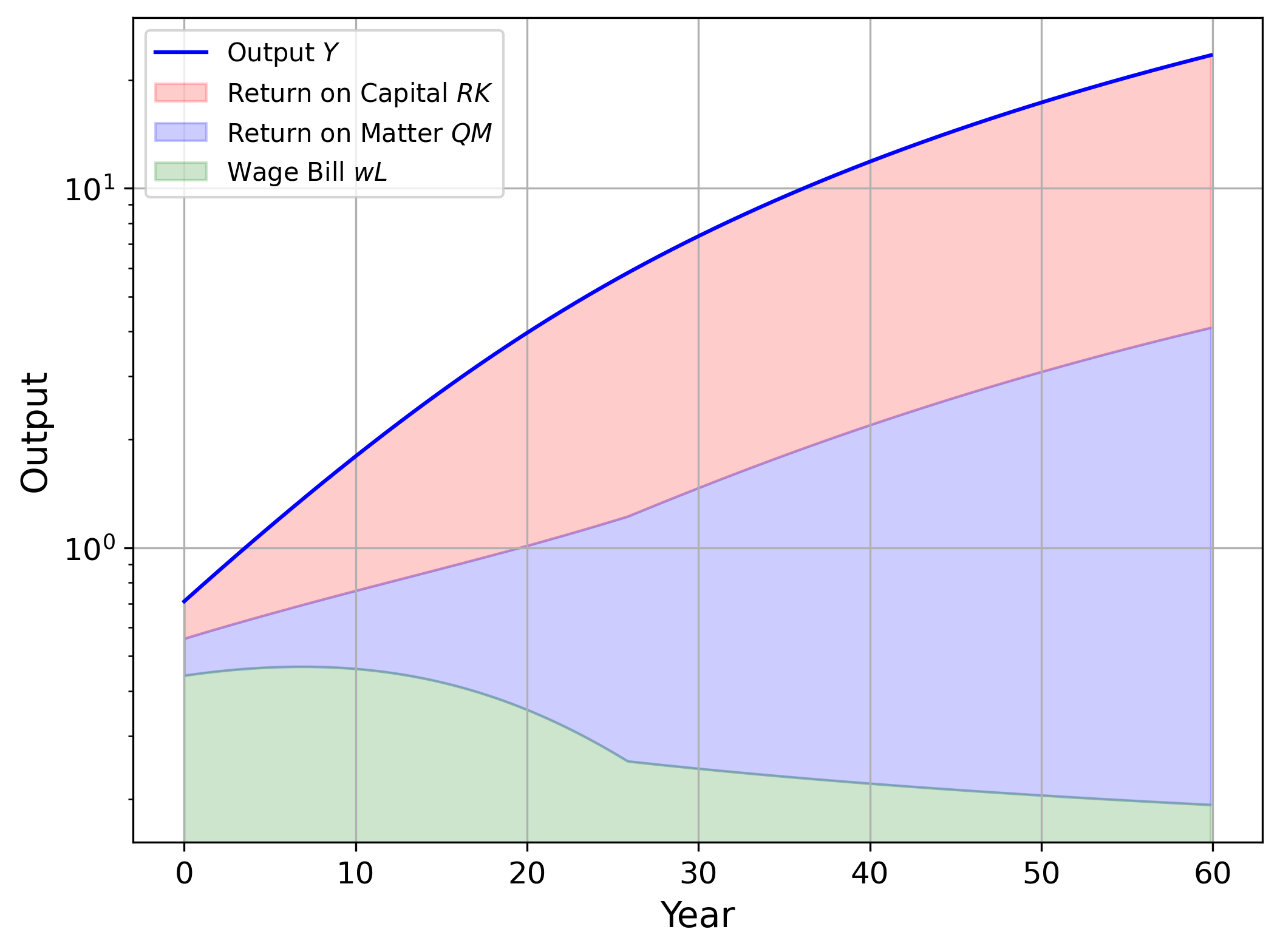
Figure 9: Factor shares with fixed factor $M$ in traditional scenario

Figure 9 illustrates the implications under the assumption that the Cobb-Douglas for $M$ is $(1-\alpha)=.10$ in the “traditional scenario,” in which a constant fraction of tasks is automated every period. As can be seen, wages peak after about 10 years, and the economy enters region 2 after 25 years, slowly converging to the steady-state level of capital $K^{\ast}$. In stark contrast to our simulation results in Section 3, this illustrates that even though there is an infinite tail of unautomated tasks, the presence of a fixed factor bottlenecks capital accumulation and implies that labor loses its scarcity status in finite time.

4.2 Automating Technological Progress

Our analysis so far has focused on automation as the only form of technological advancement and has taken as given the technology parameter $A$, which is considered as the main driver of productivity gains in the neoclassical growth model. This has allowed us to derive a number of powerful results on the effects of automation in goods production on output and wages. However, there are widespread predictions that advances in AI not only will make output production more efficient but also will speed up technological progress (Aghion et al.,, 2019; Agrawal et al.,, 2023; Davidson,, 2023).

At the most basic level, the production of R&D that drives technological progress consists of atomistic computational tasks—like any other production process described earlier in the paper. For example, Agrawal et al., (2023) suggest that scientific hypothesis generation can be viewed as the making of predictions over a vast combinatorial space. We denote the complexity distribution of tasks involved in R&D by the distribution function “Gamma” $\Gamma(i)$, which may differ from the complexity distribution of tasks $\Phi(i)$ involved in producing output—perhaps R&D involves on average more complex computational tasks. W.l.o.g., we assume that our ability to automate both R&D and production are captured by the same automation index $I$.

Building on our earlier task production function and on the endogenous growth setup of Jones, (1995), we assume that advances in the technology parameter $A$ are driven by an ideas production function combining atomistic computational tasks $\{x(i)\}$ that involve computational complexity as reflected in the distribution function $\Gamma(i)$,

$$\log\dot{A}=\log A^{\theta}+\int\log x(i)d\Gamma(i),$$

where the parameter $\theta$ captures the potential for knowledge spillovers or for decreasing returns to knowledge accumulation. Similarly with the production of final goods, we assume that automated tasks can be performed by either capital or labor whereas unautomated tasks require labor,

$$x\left(i\right)=\begin{cases}k_{A}\left(i\right)+\ell_{A}\left(i\right)&\text{for }i<I,\\ \ell_{A}\left(i\right)&\text{for }i\geq I.\end{cases}$$

To keep our analysis tractable, we assume that there is an exogenous supply of knowledge workers $L_{A}=1$ that can only work in ideas production in addition to the unit supply of workers $L_{Y}=1$ who are solely engaged in final output production. Moreover, we assume unitary elasticity of substitution between tasks in the output production function so $\sigma=1$. Analogs of lemma 1 hold for both production functions. As long as labor is scarce (region 1), we observe that the production functions of final output and knowledge satisfy $F(K,L)\simeq AK_{Y}^{\Phi(I)}L_{Y}^{1-\Phi(I)}$ and $\dot{A}\simeq A^{\theta}K_{A}^{\Gamma(I)}L_{A}^{1-\Gamma(I)}$ where $K_{Y}$ and $K_{A}$ are the aggregate amounts of capital employed in final output or knowledge production.

Following the hypothesis of Aghion et al., (2019) and the proof of Trammell and Korinek, (2023), it can then be shown that once automation in the two production functions has proceeded sufficiently, growth in the described economy will experience what Aghion et al., (2019) term a “type II singularity.” The intuition is that a rapidly growing capital stock generates an explosion in R&D output and technological progress that feeds on itself, resulting infinite output in finite time. The following proposition states this result formally under the assumptions of a constant savings rate $s\in(0,1)$, a constant allocation of capital across final output and ideas production, and no depreciation for tractability.

Proposition 11.

The economy enters a path of super-exponential growth in technology $A$ and output $Y$ that diverges to infinity in finite time once the automation index $I$ reaches the level $I^{\heartsuit}$such that

$$\frac{\Gamma\left(I^{\heartsuit}\right)}{\left(1-\Phi\left(I^{\heartsuit}\right)\right)\left(1-\theta\right)}>1$$

The marginal product of labor in the production of final output diverges to infinity alongside output.

Proof.

Observe that once the described threshold has been passed, the production functions $F(K,L)\simeq AK_{Y}^{\Phi(I^{\heartsuit})}L_{Y}^{1-\Phi(I^{\heartsuit})}$ and $\dot{A}\simeq A^{\theta}K_{A}^{\Gamma(I^{\heartsuit})}L_{A}^{1-\Gamma(I^{\heartsuit})}$ for constant fractions of capital $K_{Y}=cK$ and $K_{A}=(1-c)K$ are lower bounds for the actual production functions using the (still increasing) automation level $\Phi(I)$ and $\Gamma(I)$. The result is then a direct application of the proof in Trammell and Korinek, (2023) (Appendix B.2). Note that $w_{t}\geq A_{t}$ no matter if output production is in Region 1 or Region 2 as defined in Lemma 1. Therefore the marginal product of labor in the production of final output also diverges to infinity. ∎

The condition in the proposition depends on three parameters – sufficient automation in the production of ideas $\Gamma(\cdot)$, sufficient automation in the production of final output $\Phi(\cdot)$, and sufficient returns to the accumulation of knowledge. Remarkably, as long as the production of final output has been sufficiently automated (sufficiently high $\Phi$), the remaining two parameters can take on any finite levels. This highlights that sufficient automation in the production of final output and thus capital accumulation will always lead to an explosion in growth.

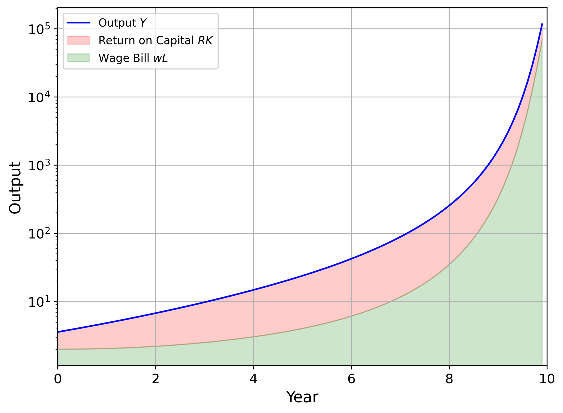
(a)

Figure 10: Output and wage growth under technological progress

Figure 10 illustrates the path of wages under a CES production function for output and optimal savings, numerically illustrating the explosive path of output growth and type-II singularity that we identified in the proposition. The convexity of the curve on a log-scale indicates that the growth rate of wages is ever-increasing due to the acceleration of technological progress. (Note that the log scale hides that the labor share of output is declining.) In the figure, we have cut off the simulation at $t=10$. The singularity occurs shortly thereafter.

In summary, even if automation induces wages to collapse to the returns to capital at $A$, rapid technological progress from the automation of R&D allows workers to benefit from the advancement of AI once sufficient automation has taken place.

More generally, the force described in this subsection is plausible, and sufficient progress in AI will likely indeed lead to rapid technological advances and increases in living standards. At the same time, it is also likely that both the production of output and of ideas will eventually be bottlenecked by fixed factors, as we emphasized in Section 4.1. A model that comprehensively incorporates both effects is beyond the scope of this paper.

4.3 Nostalgic Jobs or Limits on Automation

Our baseline model assumed that the automation of work was driven solely by technological factors, occurring as soon as the compute requirements of performing specific tasks were reached. However, even if it is technologically feasible to perform certain tasks, our society may decide that it is preferably for those tasks to remain exclusively human. For example, Korinek and Juelfs, (2023) observe that jobs such as priests, judges, or lawmakers may remain exclusively human long after the time when they can be performed at equal or superior levels by machines, labelling such jobs “nostalgic jobs.”

For the purposes of our analysis, we assume that there is a separate distribution function $\Psi(I)$ that captures how far the automation index $I$ must advance for society to choose to automate task $I$ – in addition to the distribution $\Phi\left(I\right)$ capturing the technological possibility of automation. The inequality $\Psi\left(I\right)\leq\text{$\Phi(I)$}$ reflects that society can only choose to automate tasks that are feasible to automate. The inequality is strict if there are tasks that could be automated from a technical perspective but aren’t for societal reasons. If $\lim_{I\rightarrow\infty}\Psi(I)<\Phi(I)\leq 1$, then this captures that there are tasks that humans choose to never automate even though they could be.

The described setup can also capture situations in which tasks are delegated to machines with a delay, i.e., for higher levels of the automation index $I$ than what is technologically feasible. Korinek and Juelfs, (2023) describe two reasons for why this may occur: First, as the capabilities of machines to perform certain tasks become better and better than human abilities, it may become increasingly untenable for the tasks to be left to humans. For example, if AI systems demonstrably become much fairer judges with fewer biases and noise than human judges, it may become untenable to leave many judicial deicisons to error-prone humans. Second, with sufficient advances in robotics, it may become more and more difficult to distinguish humans and AI-powered robots performing human services. They observe that a robot priest with greater emotional intelligence than humans and a more comprehensive theory of human minds than a human priest may be able to perform the tasks typically performed by human priests quite perfectly, or intentionally somewhat imperfectly so as to not give away that it is a robot. Both of these categories require that the performance of AI systems is sufficiently above human levels, corresponding to a sufficiently high level of the automation index $I$.

Maximizing Wage Growth

Consider the problem of a government with the objective to maximize wage growth by imposing limits on automation and choosing an optimal path $\Psi(I)\leq\Psi(I)$. The following result characterizes the optimal $\Psi(I)$ among all Pareto distributions—given exponential advances in the automation index $I$, this amounts to the government choosing an optimal constant rate of automation per time period.

Proposition 12 (Maximizing Wage Growth).

Suppose $\Psi$ is a Pareto distribution defined as $\Psi(I_{t})=1-I_{0}^{-\lambda}e^{-\lambda gt}$ where $I_{0}$ is the initial automation index and $\lambda g$ is the rate of task automation. Then the long-run growth rate of wages is maximized for $\lambda g=(1-\sigma)\cdot\frac{A-\rho-\delta}{\eta}$ , assuming that $\Psi(I)\leq\Psi(I)\forall I$ for this distribution. As a result, wages grow at rate $\frac{A-\rho-\delta}{\eta}$.

Proof.

The proof follows from Proposition 7. The rate of automation is lowest in case 3. And the wage growth rate is increasing in $\lambda g$. Thus, the wage growth rate increases until $\lambda g=(1-\sigma)\cdot\frac{A-\rho-\delta}{\eta}$. Once $\lambda g$ surpasses $(1-\sigma)\cdot\frac{A-\rho-\delta}{\eta}$, the growth rate of wages decreases in $\lambda g$ until $\lambda g=\frac{A-\rho-\delta}{\eta}$ at which the growth rate equals zero. Therefore, the maxmum growth rate of wages is $\frac{A-\rho-\delta}{\eta}$ at $\lambda g=(1-\sigma)\cdot\frac{A-\rho-\delta}{\eta}$. Figure 7 provides a graphical illustration of this finding—the peak of the wage growth rate as a function of $\lambda g$ is $\frac{A-\rho-\delta}{\eta}$. ∎

Figure 11 shows what happens if we slow down progress in the “baseline AGI scenario” from Section 3 so that wages growth is maximized. Up until period 14, a wage-maximizing planner is constrained by the natural pace of automation and sets $\Psi(I)=\Phi(I)$ over that stretch. After that point, the baseline AGI scenario implies rapid declines in the labor share, but the planner sets $\Psi(I)<\Phi(I)$ to slow down effective automation. The left panel of the figure shows the paths of output and wages, and the right panel depicts the two variables in relative terms for the two scenarios. Up until period 14, the paths in the two scenarios roughly coincide (with a minor gap opening since the AGI scenario triggers rapid capital accumulation in advance of the economy achieving full automation). Thereafter, the wage-maximizing planner obtains a path of exponentially growing wages, as predicted by the proposition, whereas wages in the AGI scenario collapse. Notably, the right-hand panel also illustrates the output cost of foregoing the possibility of full automation. As can be seen, the output cost of holding back automation is low at first, but eventually, almost 100% of the output potential of the economy is lost by holding back automation.

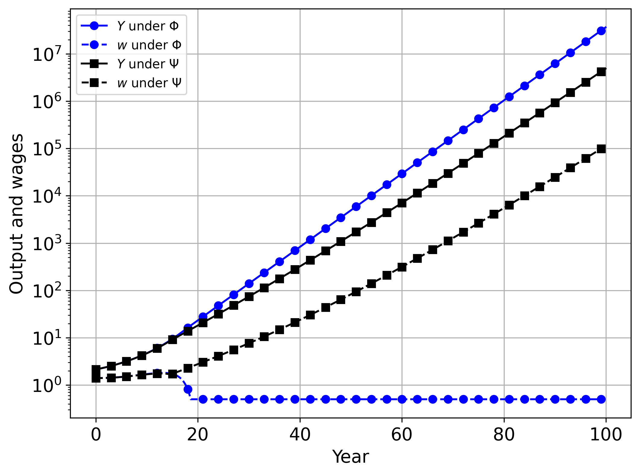
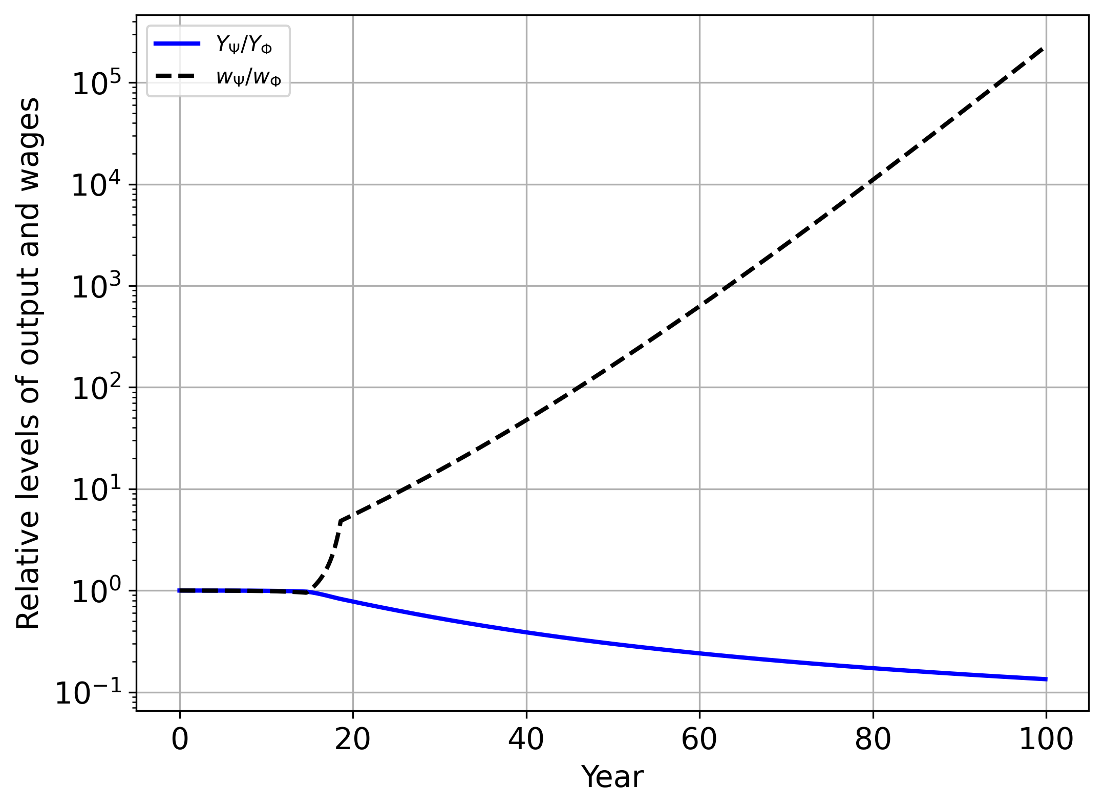
Figure 11: Comparison of output and wages under $\Phi$ and $\Psi$

Our finding illustrates that slowing down automation may be a powerful tool to increase wages, albeit it comes at the cost of reducing output growth. The described policy is feasible under both of the AGI scenarios simulated in the previous section and always results in exponentially growing wages instead of the collapse wihin a matter of years that would otherwise occur when AGI automates human tasks too quickly.

4.4 Heterogeneous Worker Skills

When labor is heterogeneous, individuals are hit by the effects of automation at different times, depending on the extent to which their skills are automated. In practice, workers differ along many different dimensions, and each worker’s labor may be complemented or substituted for in different ways by technological advances. One of the classical ways of accounting for heterogeneity in the labor market, going back to Katz and Murphy, (1992), is to split workers into skilled and unskilled based on a threshold level of educational attainment. An additional distinction, introduced by Autor et al., (2003), was to categorize workers according to whether they hold cognitive or manual jobs performing routine or non-routine activities. Under the described paradigm, we could capture the distribution of tasks in compute space separately for each of the resulting buckets (e.g., routine cognitive workers), and analyze how advances in computing capabilities will affect that type of workers. Recent advances in AI have raised the possibility that many cognitive tasks, including non-routing tasks, may be automated relatively soon (e.g. Korinek,, 2023). However, ongoing advances in robotics make it likely that non-routine manual jobs will be similarly affected to cognitive tasks by the recent wave of progress in foundation models (Ahn et al.,, 2022).

For our purposes here, we found it useful to consider labor that differs in uni-dimensional but continuous manner. We assume that workers differ in an exogenous parameter that we label skill $J$, which reflects the maximum level of task complexity that the worker can perform. Workers’ skill levels are described by the distribution function $\Upsilon(J)$. For analytical simplicity, we assume that $\Phi(I)\geq\Upsilon(I)$.

For a level of the automation index $I$, a fraction $\Upsilon(I)$ of workers are perfectly substitutable by machines and earn wage $w_{j}=A$. A fraction $1-\Upsilon(I)$ is not substitutable, but given that the remaining workers are sufficiently skilled, they are all effective substitutes for each other and earn wage $w_{j}=F_{L}\left(K+\Upsilon(I),1-\Upsilon(I)\right)$. In contrast to our baseline model, this captures the concern that automation may make workers on the lower rungs of the skill distribution redundant, whereas workers who are able to perform at higher levels of skill may benefit from automation.

In the long run, assuming less than full automation ($\Phi(I)<1$ for any finite $I$), the share of workers who are gainfully employed will decline over time and will asymptote to $1-\lim_{J\rightarrow\infty}\Upsilon(J)$, i.e., only workers who can perform unautomated tasks with arbitrary computational complexity will earn higher returns than capital. If $\Upsilon(J)=1$ for finite $J$, then the role of all human labor will lose its scarcity value in the same manner as in the AGI scenarios in our baseline model. Conversely, if $\Upsilon(J)$ asymptotes to 1, then there may be ever-growing inequality among workers: an ever-declining fraction of workers at the top may see incomes rise without bounds, whereas a fraction of the population that asymptotes towards one will see wages collapse to the level that equates the return on capital $A$.

Heterogeneity in both skill and productivity

The described setup could easily be extended to include heterogeneity in individual worker productivity in addition to heterogeneity in skill. Assume that workers not only have different skill levels $J_{j}$ but are also endowed with different efficiency units of labor $L_{j}$ per time period. This may capture, for example, that there may be two economists who can both write papers up to complexity $J$, but one of them is twice as fast at it than the other. This could explain the empirial observation that workers in the same occupation sometimes earn significantly different wages.

Complementary human capital

An alternative lens that may be relevant in the current era of cognitive automation is that workers possess different levels of human capital that is affected by automation. To keep our discussion simple, assume again that each worker $j$ is characterized by a skill level $J_{j}$ as well as an exogenous amount of human capital $H_{j}>0$, which enables them to supply $L_{j}=H_{j}$ efficiency units of labor per time period. As the automation index $I$ surpasses a given worker with skill level $J_{j}$, the human capital that they possessed is fully devalued. The loss is greater and more painful for workers with more human capital.

4.5 Compute as Specific Capital

An important feature of the ongoing AI take-off is the scarcity of compute. In our baseline model, we followed the standard neoclassical practice of modeling capital as uniform, capable of being deployed in the production of any task. As illustrated in Figure 3, automation of new tasks then implies that the existing capital stock can be smoothly allocated to a larger number of tasks, unlocking immediate productivity gains.

In practice, however, many types of capital are specific to the task for which they were created and difficult or impossible to reallocate, corresponding to what the literature has traditionally called putty-clay capital. In the current context, the most salient type of specific capital on which AI systems rely is compute, which is in very limited supply, slowing down the deployment of AI systems for new tasks. Another example of specific capital is organizational capital, including the capital derived from investments into developing new processes for deploying new technologies in firms.

We expand our framework by assuming that each unit of capital investment is specific to a task $i$ and can only be invested once the task is automated, i.e., once $I\geq i$. This leaves the task production function (2) unaffected but modifies the capital accumulation constraint: instead of a single law of motion for capital (13), the consumer needs to separately keep track of each type of capital $k\left(i\right)$ since capital that is deployed for one task cannot be redeployed later. In an economy in which automation is proceeding slowly and steadily, the consumer problem is unchanged as the resulting constraints on capital redeployment are slack—every instant of time, a density $\phi(I_{t})$ of new tasks is automated, and sufficient capital for those tasks is instantaneously accumulated. By contrast, if the economy experiences a bout of progress that leads to a discrete mass of tasks suddenly being amenable to automation, the accumulation of the relevant specific capital may lag behind. The rapid rise of LLMs at the time of writing may be an example of such a bout.

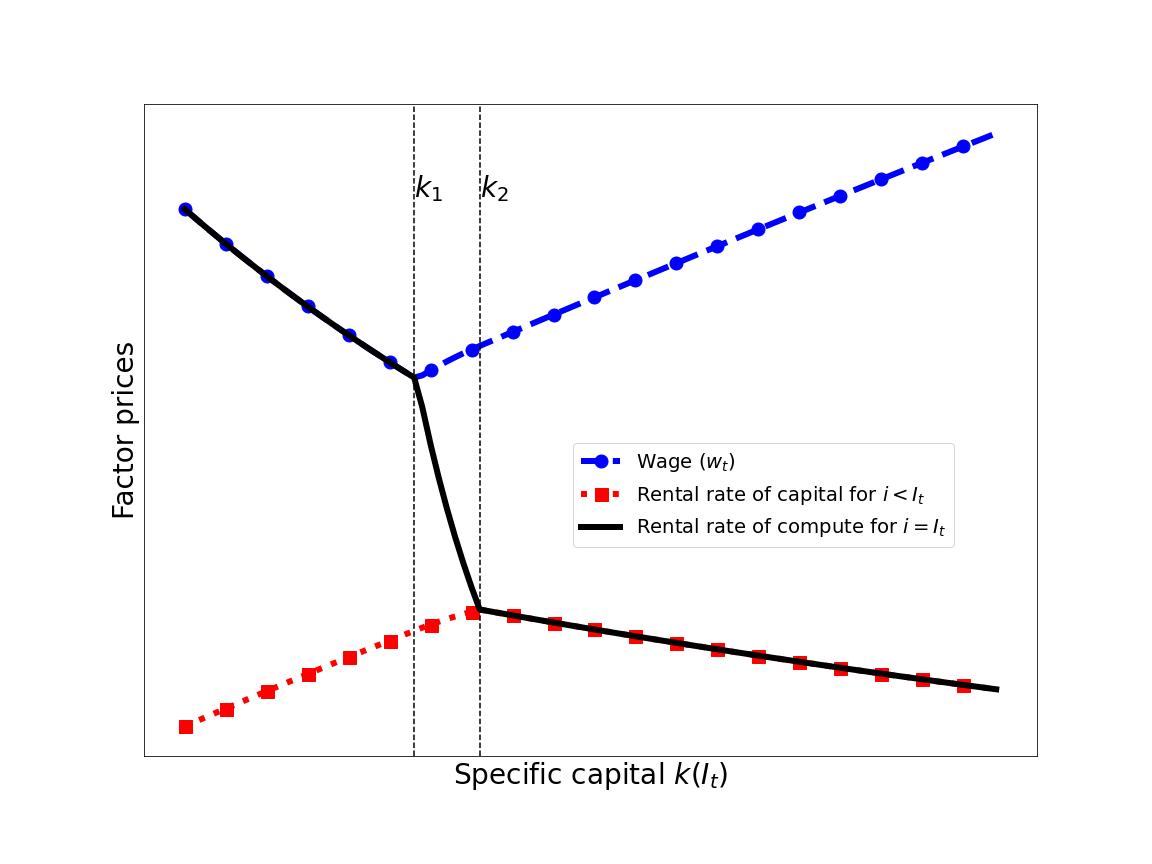
(a)

Figure 12: Specific capital and factor prices

To illustrate this analytically, assume that a discrete mass of tasks $\Delta_{t}=\Phi(I_{t})-\Phi(I_{t^{-}})>0$ is automated at time $t$, and let us interpret the specific capital $k(I_{t})$ required for these tasks as compute. At time $t$, no compute has been accumulated yet, $k(I_{t})=0$, so all type-$I_{t}$ tasks are performed by humans at wage $w$, even though they could technically be automated. Figure 12 illustrates the factor returns as a function of the accumulation of compute $k(I_{t})$ while holding the inputs of labor and other capital constant: at first, $k(I_{t})=0$, and the economy starts out at the left side of the figure where labor and compute are, at the margin, perfect substitutes so the returns on the two are equated. The rental rate on traditional capital is comparatively low.

Over time, compute capital $k(I_{t})$ is accumulated and progressively substitutes for labor. As long as compute remains below the first threshold $k(I_{t})<k_{1}$, illustrated by the first vertical line in the figure, labor and compute remain perfect substitutes at the margin, but wages $w$ decline with the addition of more compute, whereas the return on traditional capital rises. Within this region, all capital investment goes into compute. Once sufficient compute ($k_{1}$) is accumulated so that all humans are replaced from type-$I_{t}$ tasks, all labor is allocated to the remaining unautomated tasks with $i>I_{t}$, and the marginal product of compute decouples from wages. All capital investment continues to be devoted to compute; wages $w_{t}$ and the returns to traditional capital rise whereas the return on compute $k(I_{t})$ declines sharply until it reaches the marginal product of all other types of capital. This is the middle region between $k_{1}$ and $k_{2}$ where only the return on compute, captured by the dotted curve, is decreasing. Once the second threshold is passed, the marginal product of compute and other capital is equated. Any additional capital investment is spread proportionately across all types of specific capital $k(i),i\leq I$, and leads to a decline in the return on capital. In summary, the race between automation and capital accumulation leads to a non-monotonic response of wages, depicted by the blue curve marked with dots, and the returns to traditional capital, depicted by the red curve marked with squares.

The following proposition characterizes the thresholds for the amount of specific capital and summarizes the non-monotonic response of factor prices to the accumulation of this specific capital analytically.

Proposition 13 (Specific capital and factor returns).

Suppose that the current amount of the specific capital is given by $k(I_{t})$. There are threshold values $k_{1}$ and $k_{2}>k_{1}$ such that (i) if $k(I_{t})<k_{1}$ then the wage decreases and the rental rate of the traditional capital increases with $k(I_{t})$, (ii) if $k_{1}\leq k(I_{t})<k_{2}$ then both the wage and the rental rate of traditional capital increase with $k(I_{t})$, and (iii) if $k(I_{t})\geq k_{2}$ then specific capital $k(I_{t})$ is only accumulated alongside traditional capital, and the wage increases with capital accumulation.

Proof.

See appendix. ∎

In summary, rapid advances in automation may lead to episodes in which certain types of specific capital (like compute) may exhibit very high returns, but since capital is reproducible, the resulting accumulation of specific capital will ultimately dissipate the excess returns. The implication is that after an adjustment period, specific capital for newly automated processes will be just another form of capital earning the market rate of return.

5 Conclusions

This paper models the economic impact of the transition torwards artificial general intelligence on output and wages. We develop a compute-centric framework that represents work as consisting of tasks that vary in their computational complexity and study how exponential growth in computing power will affect automation and the advent of artificial general intelligence (AGI).

The paper illuminates how different plausible assumptions about the complexity distribution of tasks across "compute space" translate into dramatically different scenarios for economic outcomes. If the task distribution has an infinite Pareto tail, reflecting unlimited complexity of human work, then the we show that wages can rise indefinitely if the tail is sufficiently thick, as capital accumulation automates ever more complex tasks but there always remains enough for human labor. However, if the Pareto tail is too thin, then automation ultimately outpaces capital accumulation and causes a collapse in wages.

Moreover, if the complexity of tasks humans can perform is bounded, mirroring computational limits on human cognition, then we demonstrate that wages would at first surge as machines displace more and more human labor, but would eventually collapse, even before full AGI is reached.

Beyond these scenarios, the paper provides several powerful general insights. Using the economy’s factor price frontier, we show that the effects of automation follow an inverse U-shape, first increasing wages by utilizing abundant capital but eventually decreasing wages due to labor displacement. We show that sufficient capital accumulation is essential to prevent automation from depressing wages. Adding fixed factors like land causes wages to eventually decline. Yet automating innovation itself can restart wage growth after an initial automation-driven collapse.

The novel compute-centric approach opens up a new perspective for analyzing the economic impact of artificial intelligence. Interesting next steps include incorporating labor and capital adjustment costs, modeling endogenous innovation, analyzing distributional impacts more fully, studying macroeconomic dynamics and policies, and evaluating the possibility of an intelligence explosion with AGI.

By presenting several rigorous scenarios for how the transition to AGI may unfold, we hope that this paper will make an important contribution to enabling economists, policymakers and the public to examine alternative futures and to prepare for the technological transformations on the horizon.

Appendix A Proofs and Additional Results

A.1 Proof of Proposition 7

To begin with, we show that the growth of capital stock is approximately exponential at some constant rate. If the economy is in region 1, the production function is CES. After some algebra, the growth rate of capital is

$$\frac{\dot{K}_{t}}{K_{t}} =\frac{s_{t}A\bigg{(}K_{t}^{\frac{\sigma-1}{\sigma}}\Phi_{t}^{\frac{1}{\sigma}}+L^{\frac{\sigma-1}{\sigma}}(1-\Phi_{t})^{\frac{1}{\sigma}}\bigg{)}^{\frac{\sigma}{\sigma-1}}}{K_{t}}-\delta$$

$$=s_{t}A\bigg{(}\Phi_{t}^{\frac{1}{\sigma}}+K_{t}{}^{-\frac{\sigma-1}{\sigma}}L{}^{\frac{\sigma-1}{\sigma}}(1-\Phi_{t})^{\frac{1}{\sigma}}\bigg{)}^{\frac{\sigma}{\sigma-1}}-\delta$$

$$=s_{t}A\bigg{(}1+L^{\frac{\sigma-1}{\sigma}}\bigg{/}K_{t}{}^{\frac{\sigma-1}{\sigma}}\bigg{(}\frac{\Phi_{t}}{1-\Phi_{t}}\bigg{)}^{\frac{1}{\sigma}}\bigg{)}^{\frac{\sigma}{\sigma-1}}\cdot\Phi_{t}^{\frac{1}{\sigma-1}}-\delta$$

Note that the growth rate of capital stock depends on the behavior of $\Omega_{t}\equiv K_{t}{}^{\frac{\sigma-1}{\sigma}}\bigg{(}\frac{\Phi_{t}}{1-\Phi_{t}}\bigg{)}^{\frac{1}{\sigma}}$. In particular, $\frac{\Phi_{t}}{1-\Phi_{t}}$ grows approximately at an exponential rate under the Pareto assumption because

$$\frac{\Phi_{t}}{1-\Phi_{t}} =\frac{1-I_{t}^{-\lambda}}{I_{t}^{-\lambda}}$$

$$I_{t}^{\lambda}-1$$

$$=I_{0}^{\lambda}e^{\lambda gt}-1$$

$$\approx I_{0}^{\lambda}e^{\lambda gt}$$

We consider three cases and see whether each case is consistent with derivation above. First, suppose $\Omega_{t}\rightarrow\infty$. Then capital stock must grow at a sufficiently low rate at least for large $t$. That is, the long-run growth rate of capital $g_{K}$ must satisfy

$$g_{K}<\frac{\lambda g}{1-\sigma}$$

In this case, the growth rate of capital is

$$\frac{\dot{K}_{t}}{K_{t}} \rightarrow sA\bigg{(}1+0\bigg{)}^{\frac{\sigma}{\sigma-1}}\cdot 1-\delta$$

$$=s^{\infty}A-\delta$$

where $s^{\infty}$ is the long-run savings rate defined in Lemma 6. Then we have $g_{K}=s^{\infty}A-\delta<\frac{\lambda g}{1-\sigma}$ and thus the following upper bound on the long-run savings rate

$$s^{\infty}<\frac{1}{A}\bigg{(}\frac{\lambda g}{1-\sigma}+\delta\bigg{)}$$

Secondly, consider the case where $\Omega_{t}\rightarrow 0$. Then capital stock must grow at a rate such that

$$g_{K}>\frac{\lambda g}{1-\sigma}$$

In this case, the growth rate of capital converges to a negative value

$$\frac{\dot{K}_{t}}{K_{t}} \rightarrow sA\cdot 0\cdot 1-\delta$$

$$=-\delta$$

But this contradicts the lower bound on $g_{K}$ and puts an upper bound on the growth rate of capital stock.

Lastly, suppose $\Omega_{t}$ converges to a nonzero constant. Then it must be the case that

$$g_{K}=\frac{\lambda g}{1-\sigma}$$

which requires $\Omega_{t}\rightarrow\Omega$ where $\Omega$ is some constant satisfying $\frac{\dot{K}_{t}}{K_{t}}\rightarrow s^{\infty}A\bigg{(}1+L^{\frac{\sigma-1}{\sigma}}\bigg{/}\Omega\bigg{)}^{\frac{\sigma}{\sigma-1}}-\delta=\frac{\lambda g}{1-\sigma}$. In the three cases, capital stock grows asymptotically at either $s^{\infty}A-\delta$ or $\lambda g/(1-\sigma)$.

To characterize the long-run labor income share, note that the labor share is

$$LS_{t} =\frac{w_{t}L}{Y_{t}}$$

$$=\frac{A^{\frac{\sigma-1}{\sigma}}(Y_{t}/L)^{\frac{1}{\sigma}}(1-\Phi_{t})^{\frac{1}{\sigma}}L}{Y_{t}}$$

$$=A^{\frac{\sigma-1}{\sigma}}Y_{t}^{\frac{1}{\sigma}-1}L^{1-\frac{1}{\sigma}}(1-\Phi_{t})^{\frac{1}{\sigma}}$$

$$=A^{\frac{\sigma-1}{\sigma}}Y_{t}^{-\frac{\sigma-1}{\sigma}}L^{\frac{\sigma-1}{\sigma}}(1-\Phi_{t})^{\frac{1}{\sigma}}$$

$$=A^{\frac{\sigma-1}{\sigma}}A^{-\frac{\sigma-1}{\sigma}}\bigg{(}K_{t}^{\frac{\sigma-1}{\sigma}}\Phi_{t}^{\frac{1}{\sigma}}+L^{\frac{\sigma-1}{\sigma}}(1-\Phi_{t})^{\frac{1}{\sigma}}\bigg{)}^{-1}L^{\frac{\sigma-1}{\sigma}}(1-\Phi_{t})^{\frac{1}{\sigma}}$$

$$=\bigg{(}K_{t}^{\frac{\sigma-1}{\sigma}}\Phi_{t}^{\frac{1}{\sigma}}+L^{\frac{\sigma-1}{\sigma}}(1-\Phi_{t})^{\frac{1}{\sigma}}\bigg{)}^{-1}L^{\frac{\sigma-1}{\sigma}}(1-\Phi_{t})^{\frac{1}{\sigma}}$$

$$=\frac{L^{\frac{\sigma-1}{\sigma}}(1-\Phi_{t})^{\frac{1}{\sigma}}}{K_{t}^{\frac{\sigma-1}{\sigma}}\Phi_{t}^{\frac{1}{\sigma}}+L^{\frac{\sigma-1}{\sigma}}(1-\Phi_{t})^{\frac{1}{\sigma}}}$$

$$=\frac{L^{\frac{\sigma-1}{\sigma}}}{K_{t}^{\frac{\sigma-1}{\sigma}}\bigg{(}\frac{\Phi_{t}}{1-\Phi_{t}}\bigg{)}{}^{\frac{1}{\sigma}}+L^{\frac{\sigma-1}{\sigma}}}$$

$$=\frac{L^{\frac{\sigma-1}{\sigma}}}{\Omega_{t}+L^{\frac{\sigma-1}{\sigma}}}$$

In the first case, $\Omega_{t}\rightarrow 1$ and so $LS_{t}\rightarrow 0$. In the second case, $\Omega_{t}\rightarrow 0$ and so $LS_{t}\rightarrow 1$. Lastly, in the third case, $\Omega_{t}\rightarrow\bar{K}^{\frac{\sigma-1}{\sigma}}\bar{I}^{\frac{1}{\sigma}}$. Since $s^{\infty}A\bigg{(}1+L^{\frac{\sigma-1}{\sigma}}\bigg{/}\Omega\bigg{)}^{\frac{\sigma}{\sigma-1}}-\delta=\frac{\lambda g}{1-\sigma}$, it follows that

$$s^{\infty}A\bigg{(}1+L^{\frac{\sigma-1}{\sigma}}\bigg{/}\Omega\bigg{)}^{\frac{\sigma}{\sigma-1}}-\delta =\frac{\lambda g}{1-\sigma}$$

$$\bigg{(}1+L^{\frac{\sigma-1}{\sigma}}\bigg{/}\Omega\bigg{)}^{\frac{\sigma}{\sigma-1}} =\frac{1}{s^{\infty}A}\bigg{(}\frac{\lambda g}{1-\sigma}+\delta\bigg{)}$$

$$\bigg{(}\frac{\Omega+L^{\frac{\sigma-1}{\sigma}}}{\Omega}\bigg{)}^{\frac{\sigma}{\sigma-1}} =\frac{1}{s^{\infty}A}\bigg{(}\frac{\lambda g}{1-\sigma}+\delta\bigg{)}$$

$$\bigg{(}\frac{\Omega}{\Omega+L^{\frac{\sigma-1}{\sigma}}}\bigg{)}^{\frac{\sigma}{\sigma-1}} =\frac{s^{\infty}A}{\frac{\lambda g}{1-\sigma}+\delta}$$

$$\bigg{(}1-\frac{L^{\frac{\sigma-1}{\sigma}}}{\Omega+L^{\frac{\sigma-1}{\sigma}}}\bigg{)}^{\frac{\sigma}{\sigma-1}} =\frac{s^{\infty}A}{\frac{\lambda g}{1-\sigma}+\delta}$$

$$1-\frac{L^{\frac{\sigma-1}{\sigma}}}{\Omega+L^{\frac{\sigma-1}{\sigma}}} =\bigg{[}\frac{s^{\infty}A}{\frac{\lambda g}{1-\sigma}+\delta}\bigg{]}^{\frac{\sigma-1}{\sigma}}$$

$$\frac{L^{\frac{\sigma-1}{\sigma}}}{\Omega+L^{\frac{\sigma-1}{\sigma}}} =1-\bigg{[}\frac{s^{\infty}A}{\frac{\lambda g}{1-\sigma}+\delta}\bigg{]}^{\frac{\sigma-1}{\sigma}}$$

Therefore, $LS_{t}\rightarrow 1-\bigg{[}\frac{s^{\infty}A}{\frac{\lambda g}{1-\sigma}+\delta}\bigg{]}^{\frac{\sigma-1}{\sigma}}=1-\bigg{[}\frac{(A-\rho-\delta+\eta\delta)/\eta}{\frac{\lambda g}{1-\sigma}+\delta}\bigg{]}^{\frac{\sigma-1}{\sigma}}$.

If the economy starts in region 1 then the economy stays in region 1 as long as

$$\frac{\dot{\hat{I}}_{t}}{\hat{I}_{t}}\geq\frac{\dot{I}_{t}}{I_{t}}$$

That is, the threshold grows faster than the automation index. Under the Pareto assumption, the inequality is equivalent to

$$\frac{\dot{K}_{t}}{K_{t}}\geq\frac{1+K_{t}/L}{K_{t}/L}\cdot\lambda g$$

where $\frac{1+K_{t}/L}{K_{t}/L}$ converges to one from above. Thus, the above inequality delivers a lower bound on the savings rate for the economy to asymptotically stay in region 1:

$$s^{\infty}A-\delta>\lambda g$$ (24)

The inequality ensures that capital accumulation is sufficiently fast compared to automation. If it is violated then $I_{t}$ crosses $\hat{I}_{t}$ eventually and wages collapse to $A$.

To further examine how capital accumulation and automation shape the asymptotic behavior of wages, consider the growth rate of wages

$$\frac{\dot{w}_{t}}{w_{t}}=\frac{1}{\sigma}\frac{\dot{Y}_{t}}{Y_{t}}-\frac{1}{\sigma}\frac{\dot{\Phi}_{t}}{1-\Phi_{t}}$$

derived from $w_{t}=F_{L}$ and

$$\log F_{L} =\log A+\frac{1}{\sigma}\log(Y/A)-\frac{1}{\sigma}\log L+\frac{1}{\sigma}\log(1-\Phi(I))$$

$$\frac{d\log F_{L}}{dt} =\frac{1}{\sigma}\frac{d\log Y}{dt}+\frac{1}{\sigma}\frac{d\log(1-\Phi(I))}{dt}$$

$$=\frac{1}{\sigma}\frac{d\log Y}{dt}+\frac{1}{\sigma}\frac{1}{1-\Phi}(-\dot{\Phi})$$

. The above equation shows that the growth rate consists of output growth and the displacement effect of automation. Note that the growth rate of output is

$$\frac{\dot{Y}_{t}}{Y_{t}}=S_{K}\frac{\dot{K}_{t}}{K_{t}}+\frac{1}{1-\sigma}\frac{\dot{\Phi}_{t}}{1-\Phi_{t}}\bigg{(}S_{L}-S_{K}\frac{1-\Phi_{t}}{\Phi_{t}}\bigg{)}$$

where $S_{K}\equiv\frac{K_{t}^{\frac{\sigma-1}{\sigma}}\Phi_{t}^{\frac{1}{\sigma}}}{K_{t}^{\frac{\sigma-1}{\sigma}}\Phi_{t}^{\frac{1}{\sigma}}+L^{\frac{\sigma-1}{\sigma}}(1-\Phi_{t})^{\frac{1}{\sigma}}}$ and $S_{L}\equiv\frac{L^{\frac{\sigma-1}{\sigma}}(1-\Phi_{t})^{\frac{1}{\sigma}}}{K_{t}^{\frac{\sigma-1}{\sigma}}\Phi_{t}^{\frac{1}{\sigma}}+L^{\frac{\sigma-1}{\sigma}}(1-\Phi_{t})^{\frac{1}{\sigma}}}$, omitting time subscripts for notational simplicity. The first term is growth due to capital accumulation and the second term is growth due to the productivity effect of automation. The wage growth rate is then

$$\frac{\dot{w}_{t}}{w_{t}}=\frac{1}{\sigma}\bigg{[}S_{K}\frac{\dot{K}_{t}}{K_{t}}+\frac{1}{1-\sigma}\frac{\dot{\Phi}_{t}}{1-\Phi_{t}}\bigg{(}S_{L}-S_{K}\frac{1-\Phi_{t}}{\Phi_{t}}\bigg{)}-\frac{\dot{\Phi}_{t}}{1-\Phi_{t}}\bigg{]}$$ (25)

That is, wages rise as long as capital accumulation and the productivity effect dominate the displacement effect. In fact, this is another version of (18), which can be seen by setting $\dot{w}_{t}=0$, and tells us what determines the growth rate of wages. Under the Pareto assumption, we have

$$\frac{\dot{w}_{t}}{w_{t}}=\frac{1}{\sigma}\bigg{[}S_{K}\frac{\dot{K}_{t}}{K_{t}}+\frac{1}{1-\sigma}\cdot\lambda g\cdot\bigg{(}S_{L}-S_{K}\frac{1-\Phi_{t}}{\Phi_{t}}\bigg{)}-\lambda g\bigg{]}$$

where $\lambda g$ is the rate of automation adjusted by the decay rate of the fraction of tasks for labor.

Notice that

$$S_{K}=\frac{(*)}{(*)+L^{\frac{\sigma-1}{\sigma}}}$$

If $\lambda g>(1-\sigma)(s^{\infty}A-\delta)$ (i.e. the first case in the beginning of the proof) then $S_{K}\rightarrow 1$ since $(*)\rightarrow\infty$. Note that

$$\frac{\dot{w}_{t}}{w_{t}} =\frac{1}{\sigma}\bigg{[}S_{K}\frac{\dot{K}_{t}}{K_{t}}+\frac{1}{1-\sigma}\cdot\lambda g\cdot\bigg{(}S_{L}-S_{K}\frac{1-\Phi_{t}}{\Phi_{t}}\bigg{)}-\lambda g\bigg{]}$$

As $t\rightarrow\infty$, the growth rate of wages converges as follows

$$\frac{\dot{w}_{t}}{w_{t}} \rightarrow\frac{1}{\sigma}\bigg{[}1\cdot(s^{\infty}A-\delta)+\frac{1}{1-\sigma}\cdot\lambda g\cdot\bigg{(}0-1\cdot 0\bigg{)}-\lambda g\bigg{]}$$

$$=\frac{1}{\sigma}\bigg{[}s^{\infty}A-\delta-\lambda g\bigg{]}$$

Thus, if $s^{\infty}A-\delta>\lambda g$ (but $s^{\infty}A-\delta<\lambda g/(1-\sigma)$) then wages grow exponentially at an asymptotic rate $\frac{1}{\sigma}\bigg{[}s^{\infty}A-\delta-\lambda g\bigg{]}=\frac{1}{\sigma}\bigg{[}\frac{A-\rho-\delta}{\eta}-\lambda g\bigg{]}$.

In the case where capital stock asymptotically grows at $\lambda g/(1-\sigma)$, $S_{K}$ converges to one. As a result, the growth rate of wages converges as follows

$$\frac{\dot{w}_{t}}{w_{t}} \rightarrow\frac{1}{\sigma}\bigg{[}S_{K}\frac{\lambda g}{1-\sigma}+\frac{1}{1-\sigma}\cdot\lambda g\cdot\bigg{(}1-S_{K}-S_{K}\cdot 0\bigg{)}-\lambda g\bigg{]}$$

$$=\frac{1}{\sigma}\bigg{[}S_{K}\frac{\lambda g}{1-\sigma}+\frac{\lambda g}{1-\sigma}\cdot(1-S_{K})-\lambda g\bigg{]}$$

$$=\frac{1}{\sigma}\bigg{[}\frac{\lambda g}{1-\sigma}-\lambda g\bigg{]}$$

$$=\frac{\lambda g}{1-\sigma}$$

$$\therefore\frac{\dot{w}_{t}}{w_{t}} \rightarrow\frac{\lambda g}{1-\sigma}$$

If $s^{\infty}A-\delta\leq\lambda g$ then wages decline until the automation index crosses the threshold and collapse to $A$, as (24) indicates.

A.2 Proof of Proposition 13

Proof of Proposition 13.

The production function can be written as

$$Y_{t} =A\bigg{(}K_{t}^{\frac{\sigma-1}{\sigma}}\Phi(I_{t-})^{\frac{1}{\sigma}}+K(I)_{t}^{\frac{\sigma-1}{\sigma}}\Delta_{t}^{\frac{1}{\sigma}}+L^{\frac{\sigma-1}{\sigma}}(1-\Phi(I_{t}))^{\frac{1}{\sigma}}\bigg{)}^{\frac{\sigma}{\sigma-1}}$$

$$F_{K} =A\bigg{(}K_{t}^{\frac{\sigma-1}{\sigma}}\Phi(I_{t-})^{\frac{1}{\sigma}}+K(I)_{t}^{\frac{\sigma-1}{\sigma}}\Delta_{t}^{\frac{1}{\sigma}}+L^{\frac{\sigma-1}{\sigma}}(1-\Phi(I_{t}))^{\frac{1}{\sigma}}\bigg{)}^{\frac{1}{\sigma-1}}K_{t}^{-\frac{1}{\sigma}}\Phi(I_{t-})^{\frac{1}{\sigma}}$$

$$F_{K(I_{t})} =A\bigg{(}K_{t}^{\frac{\sigma-1}{\sigma}}\Phi(I_{t-})^{\frac{1}{\sigma}}+K(I)_{t}^{\frac{\sigma-1}{\sigma}}\Delta_{t}^{\frac{1}{\sigma}}+L^{\frac{\sigma-1}{\sigma}}(1-\Phi(I_{t}))^{\frac{1}{\sigma}}\bigg{)}^{\frac{1}{\sigma-1}}K(I)_{t}^{-\frac{1}{\sigma}}\Delta_{t}^{\frac{1}{\sigma}}$$

$$F_{L} =A\bigg{(}K_{t}^{\frac{\sigma-1}{\sigma}}\Phi(I_{t-})^{\frac{1}{\sigma}}+K(I)_{t}^{\frac{\sigma-1}{\sigma}}\Delta_{t}^{\frac{1}{\sigma}}+L^{\frac{\sigma-1}{\sigma}}(1-\Phi(I_{t}))^{\frac{1}{\sigma}}\bigg{)}^{\frac{1}{\sigma-1}}L^{-\frac{1}{\sigma}}(1-\Phi(I_{t}))^{\frac{1}{\sigma}}$$

If $F_{L}<F_{K(I_{t})}$, then the specific capital and labor are perfectly substitutable. That is,

$$\frac{K(I_{t})}{L} <\frac{\Delta_{t}}{1-\Phi(I_{t})}$$

$$k(I_{t})=\frac{K(I_{t})}{\Delta_{t}} <\frac{L}{1-\Phi(I_{t})}$$

in which case, the production function can be written as

$$Y_{t}=A\bigg{(}K_{t}^{\frac{\sigma-1}{\sigma}}\Phi(I_{t-})^{\frac{1}{\sigma}}+(K(I_{t})+L)^{\frac{\sigma-1}{\sigma}}(1-\Phi(I_{t-}))^{\frac{1}{\sigma}}\bigg{)}^{\frac{\sigma}{\sigma-1}}$$

If $F_{K}>F_{K(I_{t})}$, then the specific capital and the traditional capital are perfectly substitutable. That is,

$$\frac{K(I_{t})}{K_{t}} >\frac{\Delta_{t}}{\Phi(I_{t-})}$$

$$k(I_{t})=\frac{K(I_{t})}{\Delta_{t}} >\frac{K_{t}}{\Phi(I_{t-})}$$

in which case, the production function can be written as

$$Y_{t}=A\bigg{(}(K_{t}+K(I_{t}))^{\frac{\sigma-1}{\sigma}}\Phi(I_{t})^{\frac{1}{\sigma}}+L{}^{\frac{\sigma-1}{\sigma}}(1-\Phi(I_{t}))^{\frac{1}{\sigma}}\bigg{)}^{\frac{\sigma}{\sigma-1}}$$

∎

References

- Acemoglu and Restrepo, (2018) Acemoglu, D. and Restrepo, P. (2018). The race between machine and man: Implications of technology for growth, factor shares and employment. American Economic Review, 108(6):1488–1542.
- Acemoglu and Restrepo, (2022) Acemoglu, D. and Restrepo, P. (2022). Tasks, automation, and the rise in US wage inequality. Econometrica, 90(5):1973–2016.
- Aghion et al., (2019) Aghion, P., Jones, B., and Jones, C. (2019). Artificial intelligence and economic growth. In Agrawal, A., Gans, J., and Goldfarb, A., editors, The Economics of Artificial Intelligence: An Agenda, pages 237–290. NBER and University of Chicago Press.
- Agrawal et al., (2023) Agrawal, A. K., McHale, J., and Oettl, A. (2023). Artificial intelligence and scientific discovery: A model of prioritized search. Working Paper 31558, National Bureau of Economic Research.
- Ahn et al., (2022) Ahn, M., Brohan, A., Brown, N., Chebotar, Y., Cortes, O., and others (2022). Do as i can, not as i say: Grounding language in robotic affordances.
- Autor, (2019) Autor, D. (2019). Work of the past, work of the future. AER Papers and Proceedings, 109:1–32.
- Autor et al., (2003) Autor, D. H., Levy, F., and Murnane, R. J. (2003). The skill content of recent technological change: An empirical exploration. Quarterly Journal of Economics, 118(4):1279–1333.
- Besiroglu et al., (2022) Besiroglu, T., Emery-Xu, N., and Thompson, N. (2022). Economic impacts of AI-augmented R&D. arXiv:2212.08198.
- Bostrom, (2014) Bostrom, N. (2014). Superintelligence: Paths, Dangers, Strategies. Oxford University Press.
- Carlsmith, (2020) Carlsmith, J. (2020). How Much Computational Power Does It Take to Match the Human Brain? Open Philanthropy.
- Davidson, (2023) Davidson, T. (2023). What a compute-centric framework says about AI takeoff speeds. Working Paper.
- Eloundou et al., (2023) Eloundou, T., Manning, S., Mishkin, P., and Rock, D. (2023). GPTs are GPTs: An early look at the labor market impact potential of large language models.
- Erdil and Besiroglu, (2023) Erdil, E. and Besiroglu, T. (2023). Explosive growth from ai automation: A review of the arguments.
- Felten et al., (2023) Felten, E. W., Raj, M., and Seamans, R. (2023). How will language modelers like ChatGPT affect occupations and industries? SSRN Working Paper.
- Good, (1965) Good, I. J. (1965). Speculations concerning the first ultraintelligent machine. In Alt, F. L. and Rubinoff, M., editors, Advances in Computers, volume 6, pages 31–88. Academic Press.
- Jones, (1995) Jones, C. I. (1995). R & D-based models of economic growth. Journal of Political Economy, 103(4):759–784.
- Jones, (2023) Jones, C. I. (2023). The A.I. dilemma: Growth versus existential risk. Working Paper.
- Katz and Murphy, (1992) Katz, L. F. and Murphy, K. M. (1992). Changes in relative wages, 1963–1987: Supply and demand factors. Quarterly Journal of Economics, 107(1):35–78.
- Korinek, (2023) Korinek, A. (2023). Language models and cognitive automation for economic research. NBER Working Paper, 30957.
- Korinek and Juelfs, (2023) Korinek, A. and Juelfs, M. (2023). Preparing for the (non-existent?) future of work. In Justin Bullock et al., editor, forthcoming, Oxford Handbook of AI Governance. Oxford University Press.
- Kruppa, (2023) Kruppa, M. (2023). Google DeepMind CEO says some form of AGI possible in a few years.
- Moore, (1965) Moore, G. E. (1965). Cramming more components onto integrated circuits. Electronics Magazine, 38(8).
- Moravec, (1988) Moravec, H. (1988). Mind Children: The Future of Robot and Human Intelligence. Harvard University Press.
- Sevilla et al., (2022) Sevilla, J., Heim, L., Ho, A., Besiroglu, T., Hobbhahn, M., and Villalobos, P. (2022). Compute trends across three eras of machine learning. In 2022 International Joint Conference on Neural Networks (IJCNN), pages 1–8.
- Time, (2024) Time (2024). When might AI outsmart us? it depends who you ask. Time Magazine, page Jan. 19.
- Trammell and Korinek, (2023) Trammell, P. and Korinek, A. (2023). Economic growth under transformative AI. NBER Working Paper.
- Yudkowsky, (2013) Yudkowsky, E. (2013). Intelligence explosion microeconomics. Technical Report 2013-1, Machine Intelligence Research Institute, Berkeley, CA.
- Zeira, (1998) Zeira, J. (1998). Workers, machines, and economic growth. Quarterly Journal of Economics, 113(4):1091–1117.