Electrolubrication in flowing liquid mixtures

Abstract

We describe the “electrolubrication” occurring in liquid mixtures confined between two charged surfaces. For a mixture of two liquids, the effective viscosity decreases markedly in the presence of a field. The origin of this reduction is field-induced phase separation, leading to the formation of two low-viscosity lubrication layers at the surfaces. These layers facilitate larger strain at a given stress. The effect is strong if the viscosities of the two liquids are sufficiently different, the volume fraction of the less viscous liquid is small, the gap between the surfaces is small, and the applied potential is large. The phase separation relies on the existence of dissociated ions in the solution. The effective viscosity is reduced by a factor $\alpha$; its maximum value is the ratio between the viscosities of the two liquids. In most liquids, $\alpha\sim 1$ – $10$, and in mixtures of water and glycerol $\alpha\sim 80$ – $100$ under relatively small potentials.

I Introduction

In the electroviscous effect, the viscosity of particle suspensions depends on the particles’ charge [1, 2, 3, 4, 5, 6]. In electrorheological fluids, an external field leads to a large increase in the suspension’s viscosity [7, 8, 9, 10, 11]. In both cases, particle polarization and electrical double-layer buildup lead to long-range interactions between the particles that significantly increase the viscosity. The viscoelectric effect refers to changes in viscosity due to the effect of external electric fields on molecular dipoles in pure polar liquids. It has also been studied extensively in bulk and confined liquids, non-aqueous liquids, and water [12, 13, 14, 15, 16, 17, 18].

Room-temperature ionic liquids (RTILs) confined between surfaces have been studied extensively as potential wear-protective films in recent years. Friction forces are typically measured via an atomic force microscope [19] or surface force balance [20]. The friction force depends on molecular layering, crowding, and overscreening, often reflecting the large size of the molecules [21]. In addition, the size-asymmetry between anions and cations leads to an asymmetry between the forces measured with positively or negatively charged surfaces [22]. For moderate surface charge, the friction force between surfaces increases with electrode charge for either pure RTILs or RTILs with an added solvent [23, 24].

This paper describes a new “electrolubrication” effect occurring when liquid mixtures are confined between two plates. Here, the effective mixture’s viscosity can be reduced by applying an external potential by $1$ - $3$ orders of magnitude. The effect does not depend on specific molecular details and occurs whenever the pure liquids have different viscosities. In this phenomenon, the external potential leads to field-gradient-induced phase transition whereby a thin layer of the more polar solvent (e.g., water) adheres to the surfaces while the less polar solvent is in the center of the film [25, 26]. As shown below, when the polar solvent is the less viscous liquid, the two lubricating layers reduce the effective viscosity markedly. The transition voltage depends on the salt content, the preferential solvation of ions, temperature, and hydrophobicity/hydrophilicity of the plates [27]. The phase transition can be of first- or second-order. The effective viscosity reduction depends additionally on the ratio between the viscosities of the pure liquids, the spacing between the plates, and the relative volume fraction of the liquids.

II Model

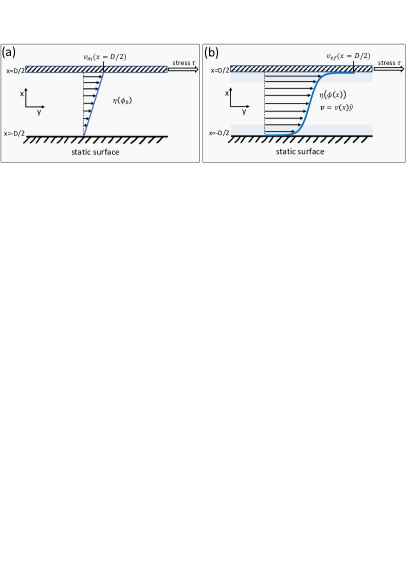
Figure 1: Schematic illustration of electrolubrication in a shear experiment. A mixture is found in the gap between two parallel and smooth surfaces. The bottom one is static and the top one is sheared at a constant stress $\tau$. (a) The mixture is homogeneous at composition $\phi_{0}$. The viscosity $\eta(\phi_{0})$ is uniform and the velocity is linear in $x$. (b) Under the influence of potential difference across the two surfaces, the mixture develops a composition profile leading to inhomogeneities of the viscosity $\eta(\phi(x))$. Two lubrication layers are created near the surfaces (shaded in faint blue), and the velocity of the top surface is significantly larger than in (a).

Consider a mixture of a polar liquid (e.g., water) and a cosolvent placed in between two flat and parallel surfaces as in Fig. 1. When the surfaces are charged, ionic screening leads to strong field gradients. Ultra-smooth surfaces whose potential can be easily adjusted were developed and used even in surface force balance experiments, where the distance between surfaces and their smoothness are crucial [28, 29, 30, 31, 32, 15] For large surface potentials, the ion density at the surfaces becomes very high, and therefore we use a modified Poisson-Boltzmann approach, employing the incompressibility constraint $\phi+\phi_{\rm cs}+v_{0}n^{-}+v_{0}n^{+}=1$, where $\phi$ and $\phi_{\rm cs}$ are the volume fractions of water and cosolvent, respectively, $v_{0}$ is the common molecular volume of all species, and $n^{\pm}$ is the number density of cations and anions. The bulk phase diagram of the mixtures in the composition-temperature $(\phi,T)$ plane is assumed to have a critical point at $(\phi_{c},T_{c})$ and a binodal curve $\phi_{b}(T)$. Liquids with partial miscibility are examined at points close to but outside the binodal, while fully miscible liquids are modeled at temperatures above $T_{c}$. We use a simple model where the bulk phase diagram in sufficiently low ionic content is symmetric around $\phi_{c}=1/2$. Thus, if the average composition $\phi=\phi_{0}$ is in the two-phase region, the equilibrium coexisting compositions, $\phi$ and $1-\phi$ are at the binodal.

II.1 Free Energy

In this section, we detail a specific realization of the energy to be used in Sec. II.2 and subsequent calculations. The grand potential is

$$\Omega[\phi(x),n^{\pm}(x),\psi(x)]=\int_{v}\biggl{[}\frac{1}{2}c^{2}\left(\nabla\phi\right)^{2}+f_{\rm m}+f_{\rm i}+f_{\rm e}$$

$$-\lambda^{+}n^{+}-\lambda^{-}n^{-}-\mu\phi/v_{0}\biggr{]}{\rm d}{\bf r}+\int_{s}f_{s}{\rm d}{\bf r}_{s}.$$ (1)

The square-gradient term accounts for the energetic cost of composition inhomogeneities, where $c^{2}=\chi/v_{0}^{1/3}$ is a positive constant. The chemical potentials of the cations and anions are $\lambda^{\pm}$, respectively, and that of the mixture is $\mu$.

The free energy density of mixing is

$$f_{\rm m} =\frac{k_{B}T}{v_{0}}\left[\phi\log(\phi)+\phi_{\rm cs}\log(\phi_{\rm cs})+\chi\phi\phi_{\rm cs}\right].$$ (2)

Here, $k_{B}$ is the Boltzmann constant, $T$ is the absolute temperature, and $\chi\sim 1/T$ is the Flory interaction parameter. Equation 2 leads to an upper critical solution temperature-type phase diagram. In the $\phi-T$ plane, a homogeneous phase is stable above the binodal curve, $\phi_{b}(T)$, whereas below it the mixture separates to water-rich and water-poor phases, with compositions given by $\phi_{b}(T)$. The two phases become indistinguishable at the critical point $(\phi_{c},\chi_{c})=(1/2,2)$.

The free energy density of the ions dissolved in the mixture, $f_{\rm i}$, is modeled as

$$f_{\rm i}= k_{B}T\bigl{[}n^{+}\log(v_{0}n^{+})+n^{-}\log(v_{0}n^{-})$$

$$-\phi(\Delta u^{+}n^{+}+\Delta u^{-}n^{-})\bigr{]},$$ (3)

The first line in Eq. (II.1) is the entropy of the ions, where $n^{\pm}$ are their number densities. The second line models the specific short-range interactions between ions and solvents, where the solvation parameters, $\Delta u^{\pm}$, measure the preference of ions toward a local water environment [33, 34, 27]. For simplicity, we take here $\Delta u^{+}=\Delta u^{-}$, i.e., both ions are equally hydrophilic.

The electrostatic energy density, $f_{\rm e}$, for a monovalent salt is given by

$$f_{\rm e}=-\frac{1}{2}\varepsilon_{0}\varepsilon(\phi)(\nabla\psi)^{2}+e(n^{+}-n^{-})\psi,$$ (4)

where $\psi$ is the electrostatic potential, $e$ is the elementary unit charge and $\varepsilon_{0}$ is the vacuum permittivity. The constitutive relation for $\varepsilon(\phi)$ is assumed to depend linearly on the mixture composition: $\varepsilon(\phi)=\varepsilon_{\rm cs}+(\varepsilon_{w}-\varepsilon_{\rm cs})\phi$, where $\varepsilon_{w}$ and $\varepsilon_{\rm cs}$ are the water and cosolvent permittivities, respectively. This $\phi$-dependence of $\varepsilon$ leads, in nonuniform electric fields, to a dielectrophoretic force which attracts the high permittivity water toward charged surfaces.

The surface energy density $f_{s}$ due to the contact of the mixture with a solid surface is given by

$$f_{s}=\Delta\gamma\phi({\bf r}_{s}),$$ (5)

where ${\bf r}_{s}$ is a vector on the surface. This expression models the short-range interaction between the fluid and the solid. The parameter $\Delta\gamma$ measures the difference between the solid–water and solid–cosolvent surface tensions. The surfaces can be hydrophilic ($\Delta\gamma<0$) or hydrophobic $(\Delta\gamma>0)$.

II.2 Flow Profiles

The viscosity of the mixture depends on $\phi$, $\phi_{\rm cs}$, and $n^{\pm}$. We denote by $\eta_{w}$ and $\eta_{\rm cs}$ the viscosities of water and cosolvent, respectively. We assume the ionic contribution to the viscosity is similar to that of the water, and hence

$$\eta=\eta_{\rm cs}\phi_{\rm cs}+\eta_{w}(1-\phi_{\rm cs}).$$ (6)

Incompressible binary mixtures in electric fields are governed by the following equations [35, 36, 37, 38, 39]:

$$\frac{\partial\phi}{\partial t}+{\bf v}\cdot\nabla\phi = L_{\phi}\nabla^{2}\frac{\delta f}{\delta\phi},$$ (7)

$$\nabla\cdot(\varepsilon_{0}\varepsilon(\phi)\nabla\psi) = -e(n^{+}-n^{-})~{},$$ (8)

$$\nabla\cdot{\bf v} = 0,$$ (9)

$$\rho\left[\frac{\partial{\bf v}}{\partial t}+({\bf v}\cdot{\bf\nabla}){\bf v}\right] = -\nabla p+\nabla\left(\eta\nabla{\bf v}+\eta(\nabla{\bf v})^{\dagger}\right)$$ (10)

$$+ {\bf f}_{\rm elec}-\phi\nabla\frac{\delta f}{\delta\phi},$$

$$\frac{\partial n^{\pm}}{\partial t}+\nabla\cdot(n{\bf v}) = L_{i}\nabla^{2}\frac{\delta f}{\delta n^{\pm}}.$$ (11)

Equation (7) is a reaction-diffusion equation including advection by the flow. ${\bf v}$ is the common velocity of the two liquids. $f=f_{\rm m}+f_{\rm i}+f_{\rm e}+(1/2)c^{2}(\nabla\phi)^{2}$ is the free energy density of the mixture. Equations (8) and (11) are the Poisson-Nernst-Planck equations. Equation (9) is the incompressibility condition and Eq. (10) is the Navier-Stokes equation, with ${\bf f}_{\rm elec}$ from Eq. (II.2) below, $p$ the pressure, and a force derivable from gradients of the chemical potential (last term on the right-hand side). The liquids’ mass density $\rho$ and the Onsager transport coefficients (mobilities) $L_{\phi}$ and $L_{i}$ are all taken here as constants independent of $\phi$ or $T$.

The body force ${\bf f}_{\rm elec}$ is given by

$${\bf f}_{\rm elec} = \frac{1}{2}\nabla\left(\varepsilon_{0}E^{2}\phi\frac{\partial\varepsilon}{\partial\phi}\right)_{T}-\frac{1}{2}\varepsilon_{0}E^{2}\nabla\varepsilon+e(n^{+}-n^{-}){\bf E},$$

where ${\bf E}=-\nabla\psi$ is the electric field.

System geometry. We focus on a simple geometry that allows significant simplification of the equations. The mixture is held in the gap between two parallel and flat surfaces located at $x=\pm D/2$, see Fig. 1. The boundary conditions for ${\bf v}$ are (i) ${\bf v}=0$ at the stationary surface at $x=-D/2$, and (ii) constant stress $\tau$ at the moving surface at $x=D/2$.

In steady-state laminar flow and for infinitely long surfaces in the $y$-direction, it follows that ${\bf v}=v(x)\hat{y}$ and all scalar quantities $\phi$, $n^{\pm}$, $\psi$ and $\eta$, depend on $x$ only. Under these conditions, the complex set of equations reduces to a much simpler one: $\phi(x)$, $n^{\pm}(x)$, and $\psi(x)$ obey the equilibrium profiles of a mixture confined by two parallel charged plates, and the velocity is given by $\eta(\phi)dv(x)/dx=\tau$.

Therefore, at a given mixture profile $\phi_{i}(x)$, the flow $v(x)$ is given by

$$v_{i}(x)=\tau\int_{x^{\prime}=-D/2}^{x}\frac{dx^{\prime}}{\eta(\phi_{i}(x^{\prime}))}.$$ (13)

The index $i$ is $i=$m for the mixed state and $i=$ef for the mixture in the electric field. We are interested in the “velocity amplification factor” $\alpha$, defined as the ratio between $v_{i}(x=D/2)$ with and without external potential: $\alpha=v_{\rm ef}(D/2)/v_{m}(D/2)$. Thus,

$$\alpha=\frac{1}{D}\int_{x=-D/2}^{x=D/2}\frac{\eta_{m}}{\eta(\phi_{\rm ef}(x))}dx.$$ (14)

Without external potential, $\phi=\phi_{0}$ and $\phi_{\rm cs}\approx 1-\phi_{0}$, provided the volume of ions is sufficiently small. The viscosity of this mixed state is $\eta_{m}=\phi_{0}\eta_{w}+(1-\phi_{0})\eta_{\rm cs}$. The velocity $v_{m}(x)=(x+D/2)\tau/\eta_{m}$ is linear in $x$, and $v_{m}(D/2)=\tau D/\eta_{m}$.

$\alpha$ could be large if, in the presence of an external field, the less viscous liquid fills the gap and expels the more viscous one. To get a significant amplification factor, one needs to have a small value of $\phi_{0}$ (more viscous liquid is a majority), large ratio $\eta_{\rm cs}/\eta_{w}$, and sufficiently large potential to induce the phase separation transition.

We now make two crude estimates of $v_{\rm ef}(D/2)$ primarily relevant for the case where water is a minority phase ($\phi_{0}<1/2$). In the first one, it is assumed that when the field is applied, two pure-water lubrication layers of thickness $w$ are formed at the surfaces. The gap between these layers is pure cosolvent. In this case

$$v_{\rm ef}(D/2)=\frac{2\tau w}{\eta_{w}}+\frac{\tau(D-2w)}{\eta_{\rm cs}}.$$ (15)

Since the velocity of the mixed state is $v_{m}(D/2)=\tau D/\eta_{m}$ and $2w/D=\phi_{0}$ we find

$$\alpha=\frac{\eta_{m}}{\eta_{\rm cs}}+\phi_{0}\left(\frac{\eta_{m}}{\eta_{w}}-\frac{\eta_{m}}{\eta_{\rm cs}}\right).$$ (16)

As a function of $\phi_{0}$, $\alpha(\phi_{0})$ is a parabola with a maximum given at $\alpha(\phi_{0}=1/2)=1/2+(1/4)(\eta_{\rm cs}/\eta_{w}+\eta_{w}/\eta_{\rm cs})$. It follows that $\alpha\gg 1$ if $\eta_{\rm cs}\gg\eta_{w}$ and if $\phi_{0}$ is not close to zero or unity. The value of $\alpha$ for a water-glycerol system ($\eta_{\rm cs}\approx 1412\eta_{w}$) with $\phi_{0}=0.2$ yields $\alpha\approx 226$. This figure overestimates the value of $\alpha$.

In the second approach, when the external potential is applied, the mixture’s composition in the gap between the two surfaces is uniform, with $\phi\approx 1-\phi_{0}$ and $\phi_{\rm cs}\approx\phi_{0}$. The viscosity is then $\eta_{\rm ef}^{\rm uni}=(1-\phi_{0})\eta_{w}+\phi_{0}\eta_{\rm cs}$. The velocity profile is linear in $x$. For the water-glycerol system with $\phi_{0}=0.2$ we find

$$\alpha=\frac{\eta_{m}}{\eta_{\rm ef}^{\rm uni}}=\frac{\phi_{0}\eta_{w}+(1-\phi_{0})\eta_{\rm cs}}{(1-\phi_{0})\eta_{w}+\phi_{0}\eta_{\rm cs}}\approx 4.$$ (17)

This figure underestimates the value of $\alpha$.

As we will see, the composition in the gap is not uniform–two thin nonuniform boundary layers are created near the surfaces. The direct effect of an electric double layer in a thin water lubricating film on the viscosity has been evaluated elsewhere [40]. This effect is relatively small compared to the electrolubrication discussed here, and consequently, we neglect it. In the water-rich layers, the cosolvent content decays to zero with the distance from the surfaces $x$. The exact function $\phi(x)$, and consequently $\eta(x)$, is essential in determining the velocity profile. In Sec. III, we calculate $\phi(x)$ and obtain the flow profile.

It is helpful to work with the dimensionless variables defined as

$$\tilde{x} = \frac{x}{\lambda_{D}},~{}~{}~{}~{}~{}~{}~{}~{}~{}~{}~{}~{}\lambda_{D}^{2}=\frac{\varepsilon_{0}\varepsilon(\phi_{0})k_{B}T}{2n_{0}e^{2}},$$

$$\tilde{\psi} = \frac{e\psi}{k_{B}T},~{}~{}~{}~{}~{}~{}~{}~{}~{}~{}~{}~{}~{}~{}\tilde{V}=\frac{eV}{k_{B}T},$$

$$\tilde{n}^{\pm} = v_{0}n^{\pm},~{}~{}~{}~{}~{}~{}~{}~{}~{}~{}~{}~{}~{}~{}\tilde{n}_{0}=v_{0}n_{0},$$

$$\tilde{c}^{2} = c^{2}\frac{v_{0}}{\lambda_{D}^{2}}\frac{1}{k_{B}T},~{}~{}~{}~{}~{}~{}~{}~{}~{}\tilde{\mu}=\frac{\mu}{k_{B}T},$$

$$\tilde{f}_{m} = \frac{v_{0}f_{m}}{k_{B}T},~{}~{}~{}~{}~{}~{}~{}~{}~{}~{}~{}~{}~{}\Delta\tilde{\gamma}=\frac{\Delta\gamma\lambda_{D}}{c^{2}}.$$ (18)

As we mentioned above, in the parallel-plates geometry, the decoupling between the direction perpendicular to the plates ($x$-direction) and parallel to them ($y$-direction) means that the quantities $\phi(x)$, $\psi(x)$ and $n^{\pm}(x)$ correspond to their equilibrium profiles. Thus, the ions obey the modified Poisson-Boltzmann distribution [27]

$$\tilde{n}^{\pm} = \frac{P^{\pm}(1-\phi)}{1+P^{+}+P^{-}},$$ (19)

$$P^{\pm} = \frac{\tilde{n}_{0}}{1-\phi_{0}-2\tilde{n}_{0}}\exp\left[(\phi-\phi_{0})(\chi+\Delta u^{\pm})\mp\tilde{\psi}\right].$$

The two remaining equations, for $\phi$ and $\tilde{\psi}$, are

$$-\tilde{c}^{2}\tilde{\nabla}^{2}\phi+\frac{\partial\tilde{f}_{m}}{\partial\phi} - \Delta u^{+}\tilde{n}^{+}-\Delta u^{-}\tilde{n}^{-}$$

$$- \frac{1}{2}\frac{2\tilde{n}_{0}}{\varepsilon(\phi_{0})}\frac{\partial\varepsilon}{\partial\phi}(\tilde{\nabla}\tilde{\psi})^{2}-\tilde{\mu}=0,$$

$$\tilde{\nabla}\cdot(\varepsilon(\phi)\tilde{\nabla}\tilde{\psi}) = \frac{\varepsilon(\phi_{0})}{2\tilde{n}_{0}}(\tilde{n}^{-}-\tilde{n}^{+}).$$ (20)

Their boundary conditions are

$$\frac{d\phi(\tilde{x}=\pm\tilde{D}/2)}{d\tilde{x}} = \mp\frac{\Delta\tilde{\gamma}}{\tilde{c}^{2}},$$

$$\tilde{\psi}(\tilde{x}=\pm\tilde{D}/2) = \pm\frac{1}{2}\tilde{V}.$$ (21)

III Results

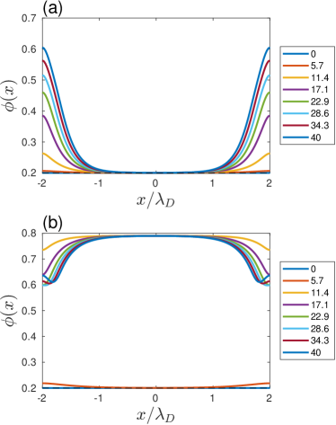
Figure 2: Composition profiles for different values of scaled potential $\tilde{V}$ (in legend) and fixed bulk composition $\phi_{0}=0.2$. (a) $\chi=0.5$ is much smaller than $\chi_{c}=2$ ($T$ is well above $T_{c}$). (b) $\chi=\chi_{b}-0.01$, where $\chi_{b}=2.31$ is the binodal for $\phi_{0}$. Unless stated otherwise, in this and in other figures, we used the parameters of water-glycerol mixtures: $\eta_{\rm cs}=\eta_{w}$, $\varepsilon_{\rm cs}=45$, and $\varepsilon_{w}=80$. In addition $\Delta u^{\pm}=3$, $\Delta\gamma=0$, $\tilde{n}_{0}=0.001$, $D=3\lambda_{D}$, and $\tilde{c}=0.4$.

We solved Eqs. (19) and (II.2) subject to their boundary conditions. The profiles $\phi(x)$ are shown in Fig. 2 for varying potentials and fixed bulk composition $\phi_{0}=0.2$. In (a) we used $\chi=0.5$, corresponding to temperatures well above $T_{c}$, simulating completely miscible liquids. At vanishing potential, the composition is uniform–$\phi(x)=\phi_{0}$–because the surfaces are taken to be neither hydrophobic nor hydrophilic ($\Delta\gamma=0$). As $\tilde{V}$ increases, a profile develops. The profiles exhibit a boundary layer at the walls ($\tilde{x}=\pm 1.5$). These layers are created due to the electrical double layer and the preferential solvation of ions in water. In (b), we used a value of $\chi$ which is close to the bulk binodal $\chi_{b}(\phi_{0})$, and increased $\tilde{V}$. While in (a) the profiles $\phi(x)$ evolve gradually with $\tilde{V}$, in (b) , they show a discontinuous jump from low $\phi(x)\approx\phi_{0}$ to high $\phi(x)\approx 0.8$ values. This is the signature of the first-order electroprewetting phase transition. At $\tilde{V}$ values above the transition, the gap between the surfaces is predominantly filled with water. As $\tilde{V}$ further increases, $\phi$ at the surfaces drops rather than increases. This drop is a result of high accumulation of ions at the surfaces; in the modified Poisson-Boltzmann framework used here, ions leave less room for water.

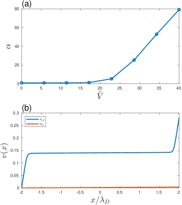
Figure 3: Electrolubrication at high temperatures $(\phi_{0},\chi)=(0.2,0.5)$. (a) $\alpha=v_{\rm ef}/v_{m}$ from Eq. (14), the ratio between the shear velocities with and without electric field, at the same shear stress, as a function of scaled potential $\tilde{V}$. (b) Velocity profiles from Eq. (13) with ($v_{\rm ef}$) and without electric field ($v_{m}$) corresponding to the last point in (a) ($\tilde{V}=25$). Velocity is in arbitrary units (we used $\tau=1$).

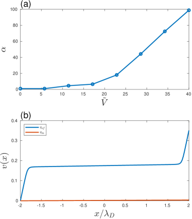
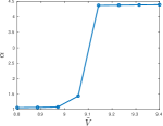
Figure 4: The same as in Fig. 3 but at low temperatures: $(\phi_{0},\chi)=(0.2,\chi_{b}-0.01)$ where $\chi_{b}=2.31$ is the binodal value for $\phi_{0}=0.2$. Inset in (a) is a zoom in the range $8.8\leq\tilde{V}\leq 9.4$, showing the discontinuity in $\alpha$.

Figures 3 and 4 show the electrolubrication effect for the two values of $\chi$ used in Fig. 2. In both figures, part (a) is a plot of $\alpha$ from Eq. (14) vs dimensionless potential $\tilde{V}$. The maximum value of $\tilde{V}$ here is $40$, corresponding to a potential of about $1$ V. By definition, $\alpha(\tilde{V}=1)=1$. $\alpha(\tilde{V})$ increases with $\tilde{V}$ due to the creation of lubrication layers near the surfaces. The thickness of these layers is a nontrivial combination of the Debye length $\lambda_{D}$ and the bulk correlation length [41]. In Fig. 3, the temperature is high $(\chi=0.5$), $\alpha(\tilde{V})$ is continuous, and reaches a value of $14$. In (b) however, the temperature is below $T_{c}$ and close to the binodal. Here $\alpha(\tilde{V})$ grows with $\tilde{V}$ until a critical potential $\tilde{V}_{c}\approx 9.1$, at which it jumps discontinuously. Inset shows enlargement of the discontinuity in $\alpha$. Above $\tilde{V}_{c}$, $\alpha(\tilde{V})$ grows continuously. The maximum value of $\alpha$, $35$, is higher compared to Fig. 3.

Parts (b) of Figs. 3 and 4 show the velocity profiles calculated by Eq. (13). Red curves show the classical linear shear profile $v_{m}(x)$ of the homogeneous mixture at the bulk composition $\phi_{0}$. The blue curves show the nonlinear velocity $v_{\rm ef}(x)$ of the inhomogeneous mixture at the maximal potential in (a) ($\tilde{V}=25$). The two lubrication layers are evident near the surfaces ($\tilde{x}=\pm 1.5$), where the gradient of $v_{\rm ef}$ is large due to the small viscosity.

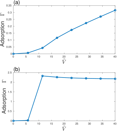
Figure 5: Adsorption $\Gamma$ from Eq. (22) as a function of $\tilde{V}$ for the two temperatures $\chi=0.5$ in (a) and $\chi=\chi_{b}-0.01$ in (b). In both parts $\phi_{0}=0.2$.

In wetting phenomena it is customary to define the adsorption $\Gamma$ as

$$\Gamma=\int_{-D/2\lambda_{D}}^{D/2\lambda_{D}}\left(\phi(\tilde{x})-\phi_{0}\right)d\tilde{x}.$$ (22)

$\Gamma$ quantifies the integrated deviation of $\phi(\tilde{x})$ from its bulk value $\phi_{0}$. Figure 5 shows the adsorption vs scaled potential $\tilde{V}$ for the low and high temperatures used in previous figures. In (a), $\chi=0.5$ and the adsorption grows continuously with $\tilde{V}$. In (b), $\chi=\chi_{b}-0.01$ is close to the binodal. Here $\Gamma(\tilde{V})$ grows continuously for small values of $\tilde{V}$. At $\tilde{V}=\tilde{V}_{c}\approx 9.1$ the first-order phase transition occurs, and $\Gamma$ jumps up. This discontinuity originates from the jump in profiles seen in Fig. 2(b). As $\tilde{V}$ further increases, $\Gamma(\tilde{V})$ gradually decreases. As mentioned above, at high surface potentials the electric double layer becomes more and more crowded, and the reduction in $\phi$ near the surfaces reduces $\Gamma$.

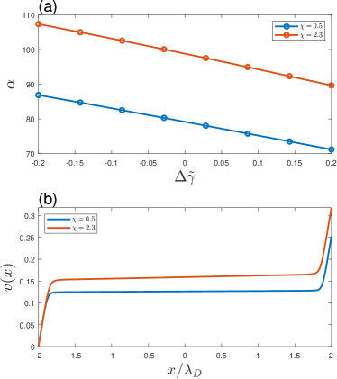
Figure 6: The influence of surface hydrophobicity/hydrophilicity on electrolubrication. (a) Flow amplification factor $\alpha$ vs $\Delta\tilde{\gamma}$ increasing from negative (hydrophilic) to positive (hydrophobic) values. The $\chi$ values (temperatures) are given in the legend. $\alpha$ decreases nearly linearly with $\Delta\tilde{\gamma}$. $\alpha$ is larger for low temperatures, closer to the binodal. (b) The flow profiles $v(x)$ when $\Delta\tilde{\gamma}=0.2$ [two rightmost points in (a)]. $v(x)$ curves are larger close to the binodal than far from it. In both parts, $\phi_{0}=0.2$ and $\chi_{b}=2.31$ for this composition.

The dependence of electrolubrication on the relative hydrophilicity/hydrophobicity of the surfaces is assessed in Fig. 6. Here, the value of $\Delta\tilde{\gamma}$ was changed between negative (hydrophilic surfaces) to positive values (hydrophobic surfaces) for two different temperatures ($\chi$ parameters) as in Figs. 3 and 4. In (a), the values of $\alpha$ are shown to decrease nearly linearly with increasing hydrophobicity. $\alpha$ is larger when the temperature is closer to the binodal ($\chi=2.3$). Part (b) shows the velocity profiles with electric fields at the two temperatures for the rightmost point in (a), i.e., for $\Delta\tilde{\gamma}=0.2$). Here again, when the mixture is closer to coexistence (red curve), $v(x)$ is larger at any point in the liquid than the high-temperature curve (blue).

IV Conclusions

Electrolubrication between two surfaces occurs when an external potential drop leads to the layering of confined liquid mixtures. The theory relies on laminar flow, an assumption valid for small surface separation $D$. The ratio between the relative velocities of the two surfaces with or without field, $\alpha$, can be quite large even at small potentials; see vertical axes in Figs. 3 and 4, recalling that $\tilde{V}=40$ corresponds to $1$ V. The lubrication effect is predicted for a wide range of temperatures and is strong even for fully miscible liquids or far from any coexistence curve [Fig. 3 (a)]. Close to a coexistence curve, the electrolubrication jumps discontinuously, as shown in the inset of Fig. 4 (a). This electrolubrication is different from the “electroactuation” in RTILs because it predicts a reduction of the effective viscosity even at small potentials and is expected to occur even in ordinary liquids.

Above, we obtained two estimates for $\alpha$, Eqs. (16) and (17). A more realistic expression can be obtained by modeling the two layers near the surfaces. Since the electric field decays nearly exponentially in the vicinity of the walls we assume that $\eta(x)$ varies as

$$\eta_{\rm ef} = \eta_{w}e^{\beta(x+D/2)}~{}~{}~{}~{}~{}-D/2\leq x\leq-D/2+w,$$

$$\eta_{\rm ef} = \eta_{\rm ef}^{\rm uni}~{}~{}~{}~{}~{}~{}~{}~{}~{}~{}~{}~{}~{}~{}~{}-D/2+w\leq x\leq D/2-w,$$

$$\eta_{\rm ef} = \eta_{w}e^{\beta(D/2-x)}~{}~{}~{}~{}~{}~{}~{}~{}D/2-w\leq x\leq D/2.$$ (23)

In this model, the viscosity in the middle of the gap $\eta_{\rm ef}^{\rm uni}$ is uniform. What is its value? In Fig. 2(b) $\phi\approx 0.8$ and the constitutive relation Eq. (6) yields $\eta_{\rm ef}^{\rm uni}\approx 285\eta_{w}$ for the water-glycerol system.

The continuity of the viscosity at $x=-D/2+w$ and $x=D/2-w$ sets the value of $\beta$ to be $\beta=w^{-1}\log\left(\eta_{\rm ef}^{\rm uni}/\eta_{w}\right)$. The velocity of the moving surface can be now readily integrated:

$$v_{\rm ef}(x=D/2)=\frac{2\tau w}{\eta_{w}}\frac{1-\eta_{w}/\eta_{\rm ef}^{\rm uni}}{\log\left(\frac{\eta_{\rm ef}^{\rm uni}}{\eta_{w}}\right)}+\frac{\tau(D-2w)}{\eta_{\rm ef}^{\rm uni}}.$$ (24)

The ratio between this velocity and $v_{m}(x=D/2)=\tau D/\eta_{m}$ is

$$\alpha=2\frac{w\eta_{m}}{D\eta_{w}}\frac{1-\eta_{w}/\eta_{\rm ef}^{\rm uni}}{\log\left(\frac{\eta_{\rm ef}^{\rm uni}}{\eta_{w}}\right)}+\frac{(1-2w/D)\eta_{m}}{\eta_{\rm ef}^{\rm uni}}.$$ (25)

Substitution of the following reasonable figures: $w/D=0.1$, $\phi_{0}=0.2$, and $\eta_{\rm cs}/\eta_{w}=1412$, yields $\alpha\approx 40$. This value is surprisingly close to the full numerical calculation [see, e.g., Fig. 4(a)] and can be important in applications where viscosity control is sought.

An interesting implementation of this effect concerns channel or pipe flow along (say) the $y$-direction, driven by a pressure gradient (stationary walls). When a homogeneous mixture enters a region in the pipe where the external potential is applied, it will demix in the $x$-direction (perpendicular to $y$). The time and length scales for this process need to be verified. If the system is translationally invariant along $y$, in steady-state, one can still decouple the $x$- and $y$-coordinates as we did here and simplify the problem significantly. Another extension of this effect relates to turbulent flow or systems lacking apparent symmetry, where layering breaks down and the two directions, parallel and perpendicular to the flow, cannot be decoupled.

Acknowledgment This work was supported by the Israel Science Foundation (ISF) via Grant No. 274/19.

References

- Booth [1950] F. Booth, The electroviscous effect for suspensions of solid spherical particles, Proceedings of the Royal Society of London. Series A. Mathematical and Physical Sciences 203, 533 (1950).
- Ren et al. [2001] L. Ren, D. Li, and W. Qu, Electro-viscous effects on liquid flow in microchannels, J. Colloid Interface Sci. 233, 12 (2001).
- Li [2001] D. Li, Electro-viscous effects on pressure-driven liquid flow in microchannels, Colloids Surf., A 195, 35 (2001).
- Anoop et al. [2009] K. Anoop, S. Kabelac, T. Sundararajan, and S. K. Das, Rheological and flow characteristics of nanofluids: Influence of electroviscous effects and particle agglomeration, J. Appl. Phys. 106, 034909 (2009).
- Rubio-Hernandez et al. [2004] F. Rubio-Hernandez, F. Carrique, and E. Ruiz-Reina, The primary electroviscous effect in colloidal suspensions, Adv. Colloid Interface Sci. 107, 51 (2004).
- Bowen and Jenner [1995] W. R. Bowen and F. Jenner, Electroviscous effects in charged capillaries, J. Colloid Interface Sci. 173, 388 (1995).
- Halsey [1992] T. C. Halsey, Electrorheological fluids, Science 258, 761 (1992).
- Hao [2001] T. Hao, Electrorheological fluids, Adv. Mater. 13, 1847 (2001).
- Stangroom [1983] J. E. Stangroom, Electrorheological fluids, Phys. Technol. 14, 290 (1983).
- Gast and Zukoski [1989] A. P. Gast and C. F. Zukoski, Electrorheological fluids as colloidal suspensions, Adv. Colloid Interface Sci. 30, 153 (1989).
- Dassanayake et al. [2000] U. Dassanayake, S. Fraden, and A. van Blaaderen, Structure of electrorheological fluids, J. Chem. Phys. 112, 3851 (2000).
- Andrade and Dodd [1939] E. d. C. Andrade and C. Dodd, Effect of an electric field on the viscosity of liquids, Nature 144, 117 (1939).
- Andrade and Dodd [1946] E. N. D. C. Andrade and C. Dodd, The effect of an electric field on the viscosity of liquids, Proceedings of the Royal Society of London. Series A. Mathematical and Physical Sciences 187, 296 (1946).
- da C Andrade and Dodd [1951] E. da C Andrade and C. Dodd, The effect of an electric field on the viscosity of liquids. ii, Proc. R. Soc. London, Ser. A 204, 449 (1951).
- Jin et al. [2022] D. Jin, Y. Hwang, L. Chai, N. Kampf, and J. Klein, Direct measurement of the viscoelectric effect in water, Proc. Natl. Acad. Sci. U.S.A. 119, e2113690119 (2022).
- Hsu et al. [2017] W.-L. Hsu, D. J. Harvie, M. R. Davidson, D. E. Dunstan, J. Hwang, and H. Daiguji, Viscoelectric effects in nanochannel electrokinetics, J. Phys. Chem. C 121, 20517 (2017).
- Sen and Barisik [2020] T. Sen and M. Barisik, Slip effects on ionic current of viscoelectric electroviscous flows through different length nanofluidic channels, Langmuir 36, 9191 (2020).
- Neogi and Ruckenstein [1981] P. Neogi and E. Ruckenstein, Viscoelectric effects in reverse osmosis, J. Colloid Interface Sci. 79, 159 (1981).
- Krämer and Bennewitz [2019] G. Krämer and R. Bennewitz, Molecular rheology of a nanometer-confined ionic liquid, J. Phys. Chem. C 123, 28284 (2019).
- Perkin [2012] S. Perkin, Ionic liquids in confined geometries, Physical Chemistry Chemical Physics 14, 5052 (2012).
- Bresme et al. [2022] F. Bresme, A. A. Kornyshev, S. Perkin, and M. Urbakh, Electrotunable friction with ionic liquid lubricants, Nature Materials 21, 848 (2022).
- Sweeney et al. [2012] J. Sweeney, F. Hausen, R. Hayes, G. B. Webber, F. Endres, M. W. Rutland, R. Bennewitz, and R. Atkin, Control of nanoscale friction on gold in an ionic liquid by a potential-dependent ionic lubricant layer, Physical review letters 109, 155502 (2012).
- Fajardo et al. [2017] O. Y. Fajardo, F. Bresme, A. A. Kornyshev, and M. Urbakh, Water in ionic liquid lubricants: friend and foe, ACS nano 11, 6825 (2017).
- Pivnic et al. [2020] K. Pivnic, F. Bresme, A. A. Kornyshev, and M. Urbakh, Electrotunable friction in diluted room temperature ionic liquids: Implications for nanotribology, ACS Applied Nano Materials 3, 10708 (2020).
- Tsori and Leibler [2007] Y. Tsori and L. Leibler, Phase-separation in ion-containing mixtures in electric fields, Proc. Natl. Acad. Sci. U.S.A. 104, 7348 (2007).
- Tsori [2021] Y. Tsori, Electroprewetting near a flat charged surface, Phys. Rev. E 104, 054801 (2021).
- Samin and Tsori [2016] S. Samin and Y. Tsori, Reversible pore gating in aqueous mixtures via external potential, Colloid Interface Sci. Commun. 12, 9 (2016).
- Zeng et al. [2008] H. Zeng, Y. Tian, T. H. Anderson, M. Tirrell, and J. N. Israelachvili, New sfa techniques for studying surface forces and thin film patterns induced by electric fields, Langmuir 24, 1173 (2008).
- Tivony et al. [2015] R. Tivony, D. B. Yaakov, G. Silbert, and J. Klein, Direct observation of confinement-induced charge inversion at a metal surface, Langmuir 31, 12845 (2015).
- Tivony and Klein [2016] R. Tivony and J. Klein, Probing the surface properties of gold at low electrolyte concentration, Langmuir 32, 7346 (2016).
- Tivony and Klein [2017] R. Tivony and J. Klein, Modifying surface forces through control of surface potentials, Faraday Discuss. 199, 261 (2017).
- Tivony et al. [2021] R. Tivony, Y. Zhang, and J. Klein, Modulating interfacial energy dissipation via potential-controlled ion trapping, J. Phys. Chem. C 125, 3616 (2021).
- Onuki and Kitamura [2004] A. Onuki and H. Kitamura, Solvation effects in near-critical binary mixtures, J. Chem. Phys. 121, 3143 (2004).
- Okamoto and Onuki [2011] R. Okamoto and A. Onuki, Charged colloids in an aqueous mixture with a salt, Phys. Rev. E 84, 051401 (2011).
- Tanaka [2000] H. Tanaka, Viscoelastic phase separation, J. Phys.: Condens. Matter 12, R207 (2000).
- Tanaka [2001] H. Tanaka, Interplay between wetting and phase separation in binary fluid mixtures: roles of hydrodynamics, J. Phys.: Condens. Matter 12, 4637 (2001).
- Ramos [2011] A. Ramos, Electrokinetics and electrohydrodynamics in microsystems, Vol. 530 (Springer Science & Business Media, 2011).
- Evans [1992] R. Evans, Fundamentals of inhomogeneous fluids (Marcel Dekker, 1992) Chap. Density functionals in the theory of nonuniform fluids, pp. 85–176.
- Tritton [2012] D. J. Tritton, Physical fluid dynamics (Springer Science & Business Media, 2012).
- Wong et al. [2003] P. Wong, P. Huang, and Y. Meng, The effect of the electric double layer on a very thin water lubricating film, Tribol. Lett. 14, 197 (2003).
- Samin and Tsori [2013] S. Samin and Y. Tsori, Stabilization of charged and neutral colloids in salty mixtures, J. Chem. Phys 139, 244905 (2013).