Local limit of massive spanning forests
on the complete graph

Abstract

We identify the local limit of massive spanning forests on the complete graph. This generalizes a well-known theorem of Grimmett on the local limit of uniform spanning trees on the complete graph.

1 Introduction and main result

Let ${G}$ be a graph without self-loops. A spanning tree of $G$ is a connected subgraph of $G$ without cycles and containing all the vertices of $G$. A spanning forest of $G$ is a subgraph of $G$ without cycles and containing all the vertices of $G$. Denote by $\mathcal{F}({G})$ the set of spanning forests of ${G}$ and for $k\geq 1$ the subset $\mathcal{F}_{k}({G})$ of spanning forests with $k$ connected components (so that $\mathcal{F}_{1}({G})$ is the set of spanning trees of $G$). A rooted spanning forest is a spanning forest with one marked vertex per connected component, also called the root of that tree. The set of rooted spanning forests is denoted by $\mathcal{F}^{\bullet}(\mathcal{G})$, and the subset of those made of $k$ trees is denoted by $\mathcal{F}^{\bullet}_{k}(\mathcal{G})$. Note that each forest $f\in\mathcal{F}_{k}(\mathcal{G})$ with connected components $t_{1},\dots,t_{k}$ corresponds to $\prod_{i=1}^{k}|t_{i}|$ rooted forests, where $|t|$ stands for the number of vertices in $t$.

For $\lambda>0$, we introduce the random $\lambda$-massive spanning forest ${\rm\bf\lambda SF}({G})$ whose distribution is defined, for all $f\in\mathcal{F}({G})$ having a set of connected components denoted by $C(f)$, by

$$\mathbf{P}\left({\rm\bf\lambda SF}(G)=f\right)\propto\lambda^{|C(f)|}\prod_{t\in C(f)}|t|\;.$$ (1)

As $\lambda\downarrow 0$, ${\rm\bf\lambda SF}(G)$ converges in distribution to ${\bf UST}(G)$. Let $\mathbf{K}_{n}$ be the complete graph with $n$ vertices and with a distinguished vertex $\mathbf{o}$. Grimmett [Gri80, Theorem 3] proved that the local limit of ${\bf UST}(\mathbf{K}_{n})$ is a Bienaymé-Galton-Watson tree with reproduction law ${\rm Poisson}(1)$, denoted by ${\rm BGWP}(1)$, conditioned to survive forever. The resulting tree $\mathcal{T}_{0}$ coincides with the random tree obtained by growing a sequence of independent unconditioned ${\rm BGWP}(1)$ on each vertex of the semi-infinite line rooted at $\mathbf{o}$. The result of Grimmett was recently extended by Nachmias–Peres [NP22, Theorem 1.1] from ${\bf UST}(\mathbf{K}_{n})$ to ${\bf UST}(G)$, where $G$ is any simple, connected, regular graph with divergent degree.

On the other hand, massive spanning forests have attracted recent attention, in relation with graph spectra in a series of work by Avena and Gaudillière [AG18a, AG18b], or with dimers and limits of near-critical trees in a work by Rey [Rey24]. A related model of cycle rooted spanning forests introduced by Kenyon [Ken11] is also investigated on increasing sequences of graph in a recent work of Constantin [Con23].

Our aim in this paper is to generalize the result of Grimmett to ${\rm\bf\lambda SF}(\mathbf{K}_{n})$. In order to state our result, we have to introduce the random tree $\mathcal{T}_{\alpha}$: for $\alpha>0$, it is obtained by growing a sequence of independent unconditioned ${\rm BGWP}(\frac{1}{1+\alpha})$ on each vertex of a spine rooted at $\mathbf{o}$ with size given by an independent random variable of law ${\rm Geom}(\frac{\alpha}{1+\alpha})$ (see Fig. 1 for a portrait).

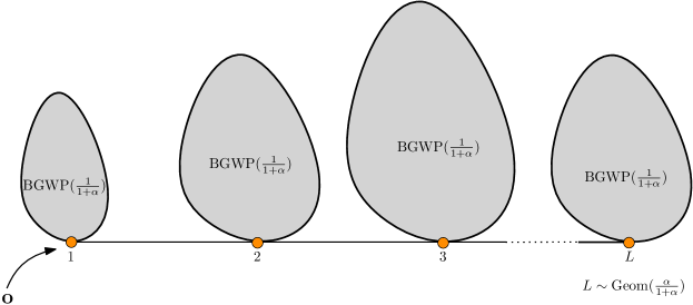
Figure 1: The distribution of the local limit $\mathcal{T}_{\alpha}$.

Let $T_{n,\lambda}$ be the connected component of $\mathbf{o}$ in ${\rm\bf\lambda SF}(\mathbf{K}_{n})$. For a given labeled tree $T$, we denote by $\text{Shape}(T,\mathbf{o})$ the non-planar unlabeled tree obtained from $T$ and rooted at $\mathbf{o}$. We endow the set of all locally finite (but possibly infinite) rooted trees with the topology inherited from the product topology. Then the convergence in distribution is called local convergence, and coincides with the convergence of probabilities that the tree cut at a finite height is equal to a given pattern. We then have the following local convergence result, for $\lambda_{n}$ depending on $n$ as $n\to\infty$:

Theorem 1 (Local limit of ${\rm\bf\lambda SF}(K_{n})$).

The following local convergence holds:

$$\emph{ \text{Shape}}(T_{n,\lambda_{n}},\mathbf{o})\underset{n\to\infty}{\overset{{\rm(d)}}{\longrightarrow}}\begin{cases}\mathcal{T}_{0}&{\rm if\;}\lambda_{n}=o(n)\\ \mathcal{T}_{\alpha}&{\rm if\;}\lambda_{n}\sim\alpha n\\ \{\mathbf{o}\}&{\rm if\;}\lambda_{n}\gg n\;.\end{cases}$$

Remark 1.1.

A corollary of 1 is that $\mathcal{T}_{\alpha}$ is unimodular.

Remark 1.2.

As shown in [CAGM18, Eq. 19], the number of connected components has mean $\frac{\lambda+1}{\lambda+n}n$ and is concentrated. When $\lambda_{n}\sim\alpha n$, this gives asymptotically $\frac{\alpha}{1+\alpha}n$. This result can be informally recovered by the computation of the expectation of the inverse of the total progeny of $\mathcal{T}_{\alpha}$, which is equal to $\frac{\alpha}{1+\alpha}$.

Acknowledgements. We thank Eleanor Archer and Lucas Rey for insightful discussions. The work of M.A. was supported by the ERC Consolidator Grant SuperGRandMA (Grant No. 101087572). N.E. was partially supported by the CNRS grant RT 2179, MAIAGES. M.A. et N.E. were partially supported by the CNRS grant RT 2173 Mathématiques et Physique, MP.

2 Determinantal properties of massive spanning forests on a graph

Let $H$ be an undirected graph without self-loops but with possibly multiple edges, denote by $V(H)$ and $E(H)$ respectively the vertex set and the edge set of $H$. Let also $n=|V(H)|$ be the size of the graph. Given two vertices $u,v\in V(H)$, we shall denote by $u\sim v$ the fact that there exists an edge connecting $u$ to $v$, and by $u\sim_{e}v$ the fact that a specific edge $e\in E(H)$ connects $u$ to $v$. For a vertex $v\in V(H)$, we shall denote by $d(v)$ the degree of $v$. Given some labeling of the vertices $\left(v_{i}\right)_{i=1}^{n}$, the adjacency matrix $A_{H}$ is defined by

$$\forall i,j=1,\ldots,n\quad\left(A_{H}\right)_{ij}\overset{\rm def}{=}|\{e\in E(H)\,;\;v_{i}\sim_{e}v_{j}\}|\,\,$$ (2.1)

and the graph Laplacian $\Delta_{H}$ is a symmetric, positive semi-definite matrix defined by

$$\forall i,j=1,\ldots,n\quad(\Delta_{H})_{ij}\overset{\rm def}{=}d(v_{i})\delta_{ij}-\left(A_{H}\right)_{ij}\,.$$ (2.2)

We denote by $P_{H}$ the characteristic polynomial of $\Delta_{H}$ defined by

$$P_{H}(\lambda)\overset{\rm def}{=}\det(\Delta_{H}+\lambda I_{n})\;.$$ (2.3)

This characteristic polynomial turns out be the partition function of spanning forests according to their number of connected components, as shown by the following celebrated Kirchhoff’s matrix-forest theorem.

Theorem 2.1 (Kirchhoff’s or Matrix-Forest Theorem [Kir47]).

Let $H$ be a graph of size $n$ without self-loops. Then

$$P_{H}(\lambda)=\sum_{k=1}^{n}\lambda^{k}|\mathcal{F}^{\bullet}_{k}(H)|=\sum_{k=1}^{n}\lambda^{k}\left[\sum_{f\in\mathcal{F}_{k}(H)}\prod_{t\in C(f)}|t|\right].$$ (2.4)

Kenyon generalized this result in [Ken11] where he described the partition function of cycle rooted spanning forests in terms of bundle Laplacian.

A consequence of this fundamental theorem is that the uniform spanning trees, and more generally the ${\rm\bf\lambda SF}$ model of spanning forests, are determinantal. This was first discovered by Burton and Pemantle in [BP93] for the uniform spanning tree case, see also the book by Lyons and Peres [LP16, Chapter 4] for an entire chapter devoted to the topic. As for spanning forests, determinantal formulas for correlations seem to have appeared sporadically. They are described in the PhD thesis of Chang [Cha13, Section 5.2] who considered the equivalent framework of spanning trees rooted at a cemetery point. Concerning the set of roots, determinantal formulas are stated by Avena and Gaudillière in [AG18b]. In this work, we need an expression of presence or absence of edges which is given by a determinant, generalizing [BP93].

For $\lambda\notin{\rm Sp}(\Delta_{H})$, consider the resolvent matrix (also called massive Green’s function)

$$R_{\lambda}=(\Delta_{H}+\lambda I_{n})^{-1}.$$ (2.5)

Using this operator on $V(H)$, we define another operator on $E(H)$ by first fixing an arbitrary orientation of the edges, so that every edge $e\in E(H)$ has an origin vertex $e_{-}$ and a target vertex $e_{+}$. Then for two edges $e,f\in E(H)$ we define

$$K_{\lambda}(e,f)=R_{\lambda}(e_{-},f_{-})+R_{\lambda}(e_{+},f_{+})-R_{\lambda}(e_{-},f_{+})-R_{\lambda}(e_{+},f_{-}).$$ (2.6)

Seen as a matrix, $K$ is called transfer current matrix. This statement says that the ${\rm\bf\lambda SF}$ model is determinantal with kernel $K_{\lambda}$.

Proposition 2.1.

Let $e_{1},\dots,e_{k},e_{k+1},\dots,e_{p}$ be $p$ distinct edges of $H$, let $\lambda>0$. Then

$${\rm\bf P}(e_{1},\dots,e_{k}\in{\rm\bf\lambda SF}(H),\ e_{k+1},\dots,e_{p}\notin{\rm\bf\lambda SF}(H))=\det M$$ (2.7)

where $M$ is the $p\times p$ matrix with entries

$$M_{i,j}=\begin{cases}K_{\lambda}(e_{i},e_{j})&\text{ if }i\leq k\\ \delta_{i,j}-K_{\lambda}(e_{i},e_{j})&\text{ if }k<i\leq p.\end{cases}$$ (2.8)

Proof.

We start with the case $k=0$, that is, we want to compute ${\rm\bf P}(e_{1},\dots,e_{p}\notin{\rm\bf\lambda SF}(H))$. Let $H\setminus\{e_{1},\dots,e_{p}\}$ be the graph obtained by deleting the edges $\{e_{1},\dots,e_{p}\}$ from $E(H)$. By Theorem 2.1, this may be expressed as

$$\frac{P_{H\setminus\{e_{1},\dots,e_{p}\}}(\lambda)}{P_{H}(\lambda)}=\frac{\det\left(\Delta_{H\setminus\{e_{1},\dots,e_{p}\}}+\lambda I_{n}\right)}{\det\left(\Delta_{H}+\lambda I_{n}\right)}.$$ (2.9)

The two involved matrices can be related in the following way. Recall that we fixed an arbitrary orientation of every edge. For any $1\leq i\leq p$, let $b_{i}$ be the vector of dimension $n=|V(H)|$ with entries $-1$ at the origin of $e_{i}$, $+1$ at the tip of $e_{i}$, and $0$ otherwise. Then we have

$$\Delta_{H\setminus\{e_{1},\dots,e_{p}\}}=\Delta_{H}-\sum_{i=1}^{p}b_{i}b_{i}^{T}=\Delta_{H}-BB^{T}$$ (2.10)

where $B$ is the $n\times p$ matrix with columns $b_{i}$. Therefore, using the Weinstein–Aronszajn identity,

$$\begin{split}\det\left(\Delta_{H\setminus\{e_{1},\dots,e_{p}\}}\right)=&\det\left(\Delta_{H}+\lambda I_{n}-BB^{T}\right)\\ =&\det\left(\Delta_{H}+\lambda I_{n}\right)\det\left(I_{n}-R_{\lambda}BB^{T}\right)\\ =&\det\left(\Delta_{H}+\lambda I_{n}\right)\det\left(I_{p}-B^{T}R_{\lambda}B\right)\end{split}$$ (2.11)

The entries of $B^{T}R_{\lambda}B$ can be seen to be equal to that of $K_{\lambda}$ by a direct computation. This concludes the proof in the case $k=0$.

For $k\geq 1$, we can write the probability of the event $\{e_{1},\dots,e_{k}\in{\rm\bf\lambda SF}{(H)},\ e_{k+1},\dots,e_{p}\notin{\rm\bf\lambda SF}{(H)}\}$ using inclusion-exclusion as a combination of probabilities of $\{e_{i_{1}},\dots,e_{i_{l}},e_{k+1},\dots,e_{p}\notin{\rm\bf\lambda SF}{(H)}\}$, and those can be expressed via the first case. It is direct to check that multi-linearity of the determinants implies the generic formula. ∎

3 A formula for the inclusion probability of a tree on $\mathbf{K}_{n}$

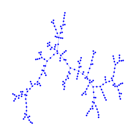
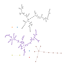
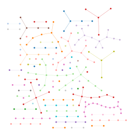
Figure 2: Samples of ${\rm\bf\lambda SF}(\mathbf{K}_{200})$ obtained via Wilson’s algorithm with a uniform, positive killing rate $r=1-\mu=\frac{\lambda}{\lambda+n-1}$. From left to right: $r=0$ (i.e. a sample of ${\bf UST}(\mathbf{K}_{200})$), $r=\frac{1}{40}$ and $r=\frac{1}{3}$.

Let $\mathbf{K}_{n}$ denote the complete graph on $n$ vertices.

Proposition 3.1 (Resolvent and transfer current matrix).

The resolvent and transfer current matrix of $\mathbf{K}_{n}$ are given by

$$R_{\lambda}(i,j)=\begin{cases}\frac{1+\lambda}{\lambda(n+\lambda)}&\text{ if }i=j\\ \frac{1}{\lambda(n+\lambda)}&\text{ if }i\neq j\end{cases}$$ (3.1)

and

$$K_{\lambda}(e,f)=\frac{1}{(n+\lambda)}\left(\mathbf{1}_{e_{-}=f_{-}}+\mathbf{1}_{e_{+}=f_{+}}-\mathbf{1}_{e_{-}=f_{+}}-\mathbf{1}_{e_{+}=f_{-}}\right)$$ (3.2)

Proof.

We start with a preparatory computation of the Green’s function of a uniform random walk $X^{\mu}_{k}$ on $\mathbf{K}_{n}$ killed at some positive rate $1-\mu$, which is equal to $G^{\mu}(x,y)=\sum_{k\geq 0}\mu^{k}\mathbf{P}_{x}(X_{k}=y)$, where $X_{k}$ denotes the uniform RW. Using the notation of Eq. 2.5, and the fact that the transition matrix of the random walk $P$ is related to the laplacian via $\Delta=(n-1)(I-P)$, we get

$$R_{\lambda}(x,y)=\frac{\mu}{n-1}G^{\mu}(x,y)\quad\mbox{where}\;\mu=\frac{n-1}{n-1+\lambda}\;.$$ (3.3)

By symmetry of the problem, we only need to compute $G^{\mu}(1,1)$ and $G^{\mu}(1,2)$. We need now to determine the distribution of $X_{k}$ conditional on $X_{0}=1$. Denoting by $x_{k}\overset{\rm def}{=}\mathbf{P}_{1}(X_{k}=1)$ and $y_{k}\overset{\rm def}{=}\mathbf{P}_{1}(X_{k}=2)$, usual Markov properties show that for $k\geq 0$,

$$\begin{cases}x_{k+1}=y_{k},\\ y_{k+1}=\frac{n-2}{n-1}y_{k}+\frac{1}{n-1}x_{k},\end{cases}$$

with $(x_{0},y_{0})=(1,0)$. From this recursion we deduce that, for all $k\geq 0$, $y_{k+1}-y_{k}=-(-\frac{1}{n-1})^{k+1}$ and using Abel transform, we get $G^{\mu}(1,2)=\sum_{k\geq 1}\mu^{k}y_{k}=\frac{n-1+\lambda}{\lambda(n+\lambda)}$, giving, via Eq. 3.3, $R_{\lambda}(1,2)=\frac{1}{\lambda(n+\lambda)}$. Since $x_{k+1}=y_{k}$, $G^{\mu}(1,1)=1+\mu G^{\mu}(1,2)$, and $R_{\lambda}(1,1)=\frac{\mu}{n-1}+\mu\,R_{\lambda}(1,2)$, which gives the formulas for $R_{\lambda}$.

From Eq. 2.6, we can write

$$K_{\lambda}(e,f)=\begin{cases}2\left(R_{\lambda}(x,x)-R_{\lambda}(x,y)\right)\text{ if }e=f\\ \left(R_{\lambda}(x,x)-R_{\lambda}(x,y)\right)\left(\mathbf{1}_{e_{-}=f_{-}}+\mathbf{1}_{e_{+}=f_{+}}-\mathbf{1}_{e_{-}=f_{+}}-\mathbf{1}_{e_{+}=f_{-}}\right)\text{ if }e\neq f\end{cases}$$ (3.4)

which leads to the formulas for $K_{\lambda}$.

∎

We can now compute the probability that a given tree is included in ${\rm\bf\lambda SF}(\mathbf{K}_{n})$:

Lemma 3.2 (Inclusion probability).

Let $t$ be a tree with vertices labeled by distinct integers in $\{1,\dots,n\}$, then

$$\mathbf{P}\left(t\subset{\rm\bf\lambda SF}(\mathbf{K}_{n})\right)=\frac{|t|}{(n+\lambda)^{|t|-1}}\;.$$

Proof.

Let $k=|t|$. Fix an orientation of $t$. From 2.1, $\mathbf{P}\left(t\subset{\rm\bf\lambda SF}(\mathbf{K}_{n})\right)=\det M_{\lambda}$, where $M_{\lambda}$ is matrix of size $(k-1)\times(k-1)$ indexed by the edges of $t$, whose entries are given by Proposition 3.1. One can check directly that

$$M_{\lambda}=\frac{1}{n+\lambda}\mathcal{A}\mathcal{A}^{T},$$

where $\mathcal{A}$ is the (rectangular) oriented incidence matrix of $t$: it has size $(k-1)\times k$, with rows indexed by the edges of $t$, columns indexed by the vertices of $t$, and whose nonzero entries are $+1$ (resp. $-1$) when the vertex is the tip (resp. origin) of the edge. Then, by the Cauchy-Binet formula,

$$\det M_{\lambda}=\frac{1}{(n+\lambda)^{k-1}}\sum_{j=1}^{k}\left(\det\mathcal{A}_{j}\right)^{2}$$

where $\mathcal{A}_{j}$ is obtained from $\mathcal{A}$ by deletion of column $j$. Then one checks directly that $\det\mathcal{A}_{j}=\pm 1$, for instance by expanding the determinant over permutations and seeing that only one permutation contributes. ∎

4 Identification of the local limit: Proof of 1

The proof comes in two steps. First, we identify the limit law of the shape of ${\rm\bf\lambda SF}(\mathbf{K}_{n})$ at a given distance $h$ from $\mathbf{o}$. Second, we show that it coincides with the distribution of $\mathcal{T}_{\alpha}$ restricted at distance $h$ from its root. These steps are the content of the following two propositions.

For a given rooted unlabeled tree $T$ and an integer $h$, we denote by:

• $T_{h}$ the set of vertices of $T$ at distance exactly $h$ from the root;

• $T_{\leq h}$ the tree given by the intersection of $T$ with the closed ball of radius $h$ centered at the root;

• $T_{<h}$ the tree given by the intersection of $T$ with the closed ball of radius $h-1$ centered at the root;

• $\text{Aut}(T)$ the set of graph automorphisms of $T$ preserving its root;

• $\mathrm{d}(u,v)$ the graph distance between vertices $u$ and $v$.

Proposition 4.1.

Let $h\in\mathbb{N}$. Let $t$ be an unlabeled tree of height $\leq h$. Then

$$\mathbf{P}\left(\emph{\text{Shape}}({\rm\bf\lambda SF}(\mathbf{K}_{n}),\mathbf{o})_{\leq h}=t\right)=\frac{1}{|\emph{\text{Aut}}(t)|}\frac{(n-1)!}{(n-|t|)!}\frac{1}{(n+\lambda)^{|t|}}\left(n|t_{h}|+\lambda|t|\right)\left(1-\frac{|t_{<h}|}{n+\lambda}\right)^{n-|t|-1}\;.$$

When $\lambda=\lambda_{n}$,

$$\lim_{n\to\infty}\mathbf{P}\left(\emph{\text{Shape}}(\lambda_{n}{\rm\bf SF}(\mathbf{K}_{n}),\mathbf{o})_{\leq h}=t\right)=\begin{cases}\frac{|t_{h}|}{|\emph{\text{Aut}}(t)|}{\rm exp}\left(-|t_{<h}|\right)&{\rm if\;}\lambda_{n}=o(n)\\ \frac{\left(|t_{h}|+\alpha|t|\right)}{|\emph{\text{Aut}}(t)|}\frac{1}{(1+\alpha)^{|t|}}{\rm exp}\left(-\frac{|t_{<h}|}{1+\alpha}\right)&{\rm if\;}\lambda_{n}\sim\alpha n\\ \delta_{t=\{\mathbf{o}\}}&{\rm if\;}\lambda_{n}\gg n\;.\end{cases}$$

Proof.

Let $T^{(n)}_{\rm lab}$ be the connected component of ${\rm\bf\lambda SF}(\mathbf{K}_{n})$ containing $\mathbf{o}$, $T^{(n)}$ its unlabeled version, $t$ as in the statement and $t_{\rm lab}$ a labeled tree whose shape is $t$. Denote the size of $t$ by $|t|(=|t_{\rm lab}|$). We wish to compute the probability of the event $T^{(n)}_{\rm lab,\leq h}=t_{\rm lab}$. This event coincides with the presence of all the edges of $t_{\rm lab}$ in $T^{(n)}_{\rm lab}$ and with the absence of all the edges joining a vertex of $t_{\rm lab,<h}$ to a vertex which does not belong to $t_{\rm lab}$ (of which there are $n-|t|$). Therefore there are $q\mathrel{\mathop{\ordinarycolon}}=|t_{\rm lab,<h}|\cdot(n-|t|)$ such absent edges, call them $e_{1},\ldots,e_{q}$. By the inclusion-exclusion principle, we can express the probability of this event only in terms of inclusion probabilities and use 3.2. Namely,

$$\begin{split}\mathbf{P}\left(T^{(n)}_{\rm lab,\leq h}=t_{\rm lab}\right)&=\mathbf{P}\left(t_{\rm lab}\subset T^{(n)}_{\rm lab,\leq h},e_{1}\notin T^{(n)}_{\rm lab},\ldots,e_{q}\notin T^{(n)}_{\rm lab}\right)\\ &=\sum_{k=0}^{q}(-1)^{k}\sum_{\begin{subarray}{c}J\subset\{1,\ldots,q\}\\ |J|=k\end{subarray}}\mathbf{P}\left(t_{\rm lab}\subset T^{(n)}_{\rm lab},\;\forall j\in J\;e_{j}\in T^{(n)}_{\rm lab}\right)\;.\end{split}$$ (4.1)

The probability appearing in the second sum on the rhs is equal to $\frac{|t|+k}{(n+\lambda)^{|t|-1+k}}$ if $t_{\rm lab}\cup\{e_{j}\,;\;j\in J\}$ is still a tree, and 0 otherwise. A cycle is formed if and only if at least two edges among $\{e_{j}\,;\;j\in J\}$ are incident at the same vertex not in $t_{\rm lab}$. Therefore, as soon as $k>n-|t|$, this probability is zero. Otherwise, there are $\binom{n-|t|}{k}$ choices of “target” vertices for the tips of $\{e_{j}\,;\;j\in J\}$ and the roots of $\{e_{j}\,;\;j\in J\}$ can be chosen freely inside $t_{\rm lab,<h}$. We thus get, after straightforward computation,

$$\begin{split}\mathbf{P}\left(T^{(n)}_{\rm lab,\leq h}=t_{\rm lab}\right)&=\sum_{k=0}^{n-|t|}(-1)^{k}\binom{n-|t|}{k}|t_{<h}|^{k}\frac{|t|+k}{(n+\lambda)^{|t|-1+k}}\\ &=\frac{1}{(n+\lambda)^{|t|}}\left(n|t_{h}|+\lambda|t|\right)\left(1-\frac{|t_{<h}|}{n+\lambda}\right)^{n-|t|-1}\;.\end{split}$$ (4.2)

Lastly, we want to compute $\mathbf{P}\left({\text{Shape}}({\rm\bf\lambda SF}(\mathbf{K}_{n}),\mathbf{o})_{\leq h}=t\right)$. For each labeling ${\bf l}$ of $t$, there are exactly $|\text{Aut}(t)|$ labelings ${\bf l^{\prime}}$ for which the events $\{T^{(n)}_{{\rm lab},\leq h}=t_{{\bf l}}\}$ and $\{T^{(n)}_{{\rm lab},\leq h}=t_{{\bf l^{\prime}}}\}$ are the same. On the other hand, there are $\frac{(n-1)!}{(n-|t|)!}$ possible labelings. This concludes the proof for $n$ fixed, and the limits are straightforward.
∎

We turn to the second step, where we study the limiting random tree $\mathcal{T}_{\alpha}$. We start with a preliminary lemma on standard subcritical $\text{BGWP}(\beta)$.

Lemma 4.2.

Let $\beta<1$, let $h\in\mathbb{N}$. Let $t$ be an unlabeled tree of height $\leq h$.

$$\mathbf{P}\left(\emph{\text{BGWP}}(\beta)_{\leq h}=t\right)=\frac{1}{|\emph{\text{Aut}}(t)|}\beta^{|t|-1}e^{-\beta|t_{<h}|}\;.$$

Proof.

We compare the recursion relations satisfied by both quantities. We group the children of the root in equivalence classes: two children are in the same class if and only if they are the root of isomorphic subtrees. We denote now by $\ell$ the number of equivalence classes, and by $n_{1},\ldots,n_{l}$ their cardinality. Since the number of children of the root is $\text{Poisson}(\beta)$ distributed, we can write

$$\begin{split}\mathbf{P}\left({\text{BGWP}}(\beta)_{\leq h}=t\right)&=\frac{\beta^{n_{1}+\cdots+n_{l}}e^{-\beta}}{(n_{1}+\cdots+n_{l})!}\binom{n_{1}+\cdots+n_{l}}{n_{1},\ldots,n_{l}}\prod_{i=1}^{l}\mathbf{P}\left({\text{BGWP}}(\beta)_{\leq h-1}=t_{i}\right)^{n_{i}}\\ &=\frac{\beta^{n_{1}+\cdots+n_{l}}e^{-\beta}}{n_{1}!\cdots n_{l}!}\prod_{i=1}^{l}\mathbf{P}\left({\text{BGWP}}(\beta)_{\leq h-1}=t_{i}\right)^{n_{i}}\end{split}$$ (4.3)

where $t_{i}$ is the subtree of $t$ emanating from a child of the root belonging to the $i$-th equivalence class. On the other hand, $|{\text{Aut}}(t)|$ satisfies the recursion

$$|{\text{Aut}}(t)|=\prod_{i=1}^{l}n_{i}!|{\text{Aut}}(t_{i})|^{n_{i}}$$

hence if we denote by $f$ the function on finite trees which maps $t$ onto $f(t)=\frac{1}{|{\text{Aut}}(t)|}\beta^{|t|-1}e^{-\beta|t_{<H(t)}|}$, where $H(t)$ is the height of $t$,

$$\frac{\beta^{n_{1}+\cdots+n_{l}}e^{-\beta}}{n_{1}!\cdots n_{l}!}\prod_{i=1}^{l}f(t_{i})^{n_{i}}=\frac{\beta^{n_{1}+\cdots+n_{l}}e^{-\beta}}{n_{1}!\cdots n_{l}!}\prod_{i=1}^{l}\left(\frac{1}{|{\text{Aut}}(t_{i})|}\beta^{|t_{i}|-1}e^{-\beta|t_{i,<H(t_{i})}|}\right)^{n_{i}}=f(t)\;.$$ (4.4)

Equations 4.3 and 4.4 show that both quantities of the statement satisfy the same recursion. ∎

We can now identify the distribution of ${\text{Shape}}{(\mathcal{T}_{\alpha},\mathbf{o})}$:

Proposition 4.3.

Let $h\in\mathbb{N}$. Let $t$ be an unlabeled tree of height $\leq h$. Then

$$\mathbf{P}\left(\emph{\text{Shape}}{(\mathcal{T}_{\alpha},\mathbf{o})}_{\leq h}=t\right)=\frac{|t_{h}|+\alpha|t|}{|\emph{\text{Aut}}(t)|}\frac{1}{(1+\alpha)^{|t|}}{\rm exp}\left(-\frac{|t_{<h}|}{1+\alpha}\right)\;.$$

Proof.

We decompose the probability according to the position of the vertex $v$ of the spine which is the farthest from $\mathbf{o}$. Let us denote by $[v]$ its equivalence class in the quotient of $t$ by the action of $\text{Aut}(t)$. The vertex $v$ might be at distance $h$ or not; in any case, the probability given that $v$ satisfies our requirement depends only on $[v]$. Calling $L$ the cardinality of the spine, we will use the relation $\mathbf{P}\left(L\geq h\right)=\left(\frac{1}{1+\alpha}\right)^{h}$ when $v\in t_{h}$ and the relation $\mathbf{P}\left(L=k+1\right)=\frac{\alpha}{(1+\alpha)^{k+1}}$ when $\mathrm{d}(v,\mathbf{o})=k$. Calling $t_{i,v}$ the tree growing from the $i$-th vertex of the spine, we have

$$\begin{split}\mathbf{P}\left({\text{Shape}}{(\mathcal{T}_{\alpha},\mathbf{o})}_{\leq h}=t\right)&=\sum_{[v]\in t_{h}/\text{Aut}(t)}\left[\prod_{i=0}^{h}\mathbf{P}\left({\text{BGWP}}\left(\frac{1}{1+\alpha}\right)_{h-i+1}=t_{i,v}\right)\right]\left(\frac{1}{1+\alpha}\right)^{h}+\\ &+\sum_{[v]\in t_{<h}/\text{Aut}(t)}\left[\prod_{i=0}^{\mathrm{d}({v},\mathbf{o})}\mathbf{P}\left({\text{BGWP}}\left(\frac{1}{1+\alpha}\right)_{h-i+1}=t_{i,v}\right)\right]\frac{\alpha}{(1+\alpha)^{\mathrm{d}(v,\mathbf{o})+1}}\;.\end{split}$$ (4.5)

We use 4.2 with $\beta=\frac{1}{1+\alpha}$. Note that

$$(1+\alpha)^{|t_{1,v}|-1}\cdots(1+\alpha)^{|t_{h,v}|-1}(1+\alpha)^{\mathrm{d}(v,\mathbf{o})}=(1+\alpha)^{|t|},$$

which gives

$$\begin{split}\mathbf{P}\left({\text{Shape}}{(\mathcal{T}_{\alpha},\mathbf{o})}_{\leq h}=t\right)&=\sum_{[v]\in t_{h}/\text{Aut}(t)}\frac{{\rm exp}\left(-\frac{|t_{<h}|}{1+\alpha}\right)}{(1+\alpha)^{|t|}}\prod_{i=0}^{h}\frac{1}{|\text{Aut}(t_{i,v})|}+\\ &+\frac{\alpha}{1+\alpha}\sum_{[v]\in t_{<h}/\text{Aut}(t)}\frac{{\rm exp}\left(-\frac{|t_{<h}|}{1+\alpha}\right)}{(1+\alpha)^{|t|}}\prod_{i=0}^{\mathrm{d}(v,\mathbf{o})}\frac{1}{|\text{Aut}(t_{i,v})|}\;.\end{split}$$ (4.6)

To conclude, we use the Burnside lemma for the action of Aut on $t_{h}$ and on $t_{<h}$, giving

$$|t_{h}|=\displaystyle\sum_{[v]\in t_{h}/\text{Aut}(t)}|\text{Aut}(t)|\prod_{i=0}^{h}\frac{1}{|\text{Aut}(t_{i,v})|}\text{ and }|t_{<h}|=\displaystyle\sum_{[v]\in t_{<h}/\text{Aut}(t)}|\text{Aut}(t)|\prod_{i=0}^{\mathrm{d}({v},\mathbf{o})}\frac{1}{|\text{Aut}(t_{i,{v}})|},$$

and the statement follows.

∎

References

• [AG18a] Luca Avena and Alexandre Gaudillière. A proof of the transfer-current theorem in absence of reversibility. Statistics & Probability Letters, 142:17–22, 2018.
• [AG18b] Luca Avena and Alexandre Gaudillière. Two Applications of Random Spanning Forests. Journal of Theoretical Probability, 31(4):1975–2004, December 2018.
• [BP93] Robert Burton and Robin Pemantle. Local characteristics, entropy and limit theorems for spanning trees and domino tilings via transfer-impedances. The Annals of Probability, 21(3):1329–1371, 1993.
• [CAGM18] Fabienne Castell, Luca Avena, Alexandre Gaudilliere, and Clothilde Melot. Random Forests and Networks Analysis. Journal of Statistical Physics, August 2018.
• [Cha13] Yinshan Chang. Contribution à l’étude des lacets markoviens. Phd thesis, Université Paris Sud - Paris XI, June 2013.
• [Con23] Héloïse Constantin. Sampling random cycle-rooted spanning forests on infinite graphs. arXiv preprint arXiv:2308.09425, 2023.
• [Gri80] Geoffrey R. Grimmett. Random labelled trees and their branching networks. Journal of the Australian Mathematical Society, 30(2):229–237, 1980.
• [Ken11] Richard Kenyon. Spanning forests and the vector bundle Laplacian. The Annals of Probability, 39(5):1983 – 2017, 2011.
• [Kir47] Gustav R. Kirchhoff. Ueber die Auflösung der Gleichungen, auf welche man bei der Untersuchung der linearen Vertheilung galvanischer Ströme geführt wird. Annalen der Physik, 148:497–508, 1847.
• [LP16] Russell Lyons and Yuval Peres. Probability on Trees and Networks, volume 42 of Cambridge Series in Statistical and Probabilistic Mathematics. Cambridge University Press, New York, 2016. Available at https://rdlyons.pages.iu.edu/.
• [NP22] Asaf Nachmias and Yuval Peres. The local limit of uniform spanning trees. Probability Theory and Related Fields, 182(3-4):1133–1161, 2022.
• [Rey24] Lucas Rey. The Doob transform and the tree behind the forest, with application to near-critical dimers. arXiv preprint arXiv:2401.13599, 2024.