A path-dependent PDE solver based on signature kernels

Abstract.

We develop a provably convergent kernel-based solver for path-dependent PDEs (PPDEs). Our numerical scheme leverages signature kernels, a recently introduced class of kernels on path-space. Specifically, we solve an optimal recovery problem by approximating the solution of a PPDE with an element of minimal norm in the signature reproducing kernel Hilbert space (RKHS) constrained to satisfy the PPDE at a finite collection of collocation paths. In the linear case, we show that the optimisation has a unique closed-form solution expressed in terms of signature kernel evaluations at the collocation paths. We prove consistency of the proposed scheme, guaranteeing convergence to the PPDE solution as the number of collocation points increases. Finally, several numerical examples are presented, in particular in the context of option pricing under rough volatility. Our numerical scheme constitutes a valid alternative to the ubiquitous Monte Carlo methods.

1. Introduction

1.1. Path-dependent PDEs

The Feynman-Kac formula asserts that solutions to backward Kolmogorov equations have a probabilistic representation as $u_{0}(t,x)=\mathbb{E}[\phi(Y_{T})\lvert Y_{t}=x]$, for $0\leq t\leq T,\,x\in\mathbb{R}^{d}$, where $Y$ is an underlying Markov process. If $Y$ models the evolution of a financial asset price, then this expectation corresponds to the price of a European-type derivative written on this asset. In its seminal paper, Dupire [21] introduces a first generation of path-dependent PDEs (PPDE) which solution is represented as $u_{1}(t,\gamma)=\mathbb{E}[\phi(Y_{[0,T]})\lvert Y_{[0,t]}=\gamma]$ where $\phi$ acts on the whole past of $Y$ and $\gamma$ is a path. This expectation represents the price of a path-dependent derivative. Rough volatility models, and more generally stochastic Volterra processes, are not Markov processes hence neither formulation applies. The recent framework of [52] tackles precisely this class of processes, for which the path-dependence is inherent to the dynamics. We illustrate this with an example to highlight the differences with the aforementioned cases. Let us consider a one factor rough volatility model

(1.1) $$X_{t}=X_{0}+\int_{0}^{t}\sqrt{\psi_{s}(\widehat{W}_{s})}\,\mathrm{d}B_{s}-\frac{1}{2}\int_{0}^{t}\psi_{s}(\widehat{W}_{s})\,\mathrm{d}s,\qquad\widehat{W}_{t}:=\int_{0}^{t}K(t,r)\,\mathrm{d}W_{r},$$

where $B$ and $W$ are correlated Brownian motions and generate their natural filtration $(\mathcal{F}_{t})_{t\in[0,T]}$, the kernel $K$ is square integrable and typically taken to be $K(t,r)=(t-r)^{H-\frac{1}{2}},\,H\in(0,1/2)$. In this situation, $\widehat{W}$ is a Gaussian Volterra process, which is neither a semimartingale nor a Markov process, hence why classical tools are not suitable. For $s\geq t$, we make the orthogonal decomposition $\widehat{W}_{s}=\Theta^{t}_{s}+I^{t}_{s}$ where $\Theta^{t}_{s}=\int_{0}^{t}K(s,r)\,\,\mathrm{d}W_{r}$ is $\mathcal{F}_{t}$-measurable while $I^{t}_{s}=\int_{t}^{s}K(s,r)\,\,\mathrm{d}W_{r}$ is independent from $\mathcal{F}_{t}$. As a consequence one recovers the Markovian structure

$$\mathbb{E}[\phi(X_{T})|\mathcal{F}_{t}] =\mathbb{E}\left[\phi\left(X_{t}+\int_{t}^{T}\sqrt{\psi_{s}(\widehat{W}_{s})}\,\mathrm{d}B_{s}-\frac{1}{2}\int_{t}^{T}\psi_{s}(\widehat{W}_{s})\,\mathrm{d}s\right)\Big{\lvert}\mathcal{F}_{t}\right]$$

$$=\mathbb{E}\left[\phi\left(X_{t}+\int_{t}^{T}\sqrt{\psi_{s}(\Theta^{t}_{s}+I^{t}_{s})}\,\mathrm{d}B_{s}-\frac{1}{2}\int_{t}^{T}\psi_{s}(\Theta^{t}_{s}+I^{t}_{s})\,\mathrm{d}s\right)\Big{\lvert}\mathcal{F}_{t}\right]$$

$$=\mathbb{E}\left[\phi\left(x+\int_{t}^{T}\sqrt{\psi_{s}(\gamma_{s}+I^{t}_{s})}\,\mathrm{d}B_{s}-\frac{1}{2}\int_{t}^{T}\psi_{s}(\gamma_{s}+I^{t}_{s})\,\mathrm{d}s\right)\Big{\lvert}X_{t}=x,\Theta^{t}=\gamma_{[t,T]}\right]$$

$$=\mathbb{E}\left[\phi(X_{T})|X_{t},\Theta^{t}_{[t,T]}\right],$$

The path-dependence of the option price is now clear and entails there is a measurable map $u_{2}$ such that $u_{2}(t,x,\gamma)=\mathbb{E}\left[\phi(X_{T})|X_{t}=x,\Theta^{t}=\gamma_{[t,T]}\right]$. Building on Viens and Zhang’s functional Itô formula, further works [10, 53] study the associated path-dependent PDE of second generation of the form

(1.2) $$\left\{\begin{array}[]{rl}&\mathcal{L}u(t,x,\gamma)=0,\\ &u(T,x,\gamma)=\phi(x),\end{array}\right.$$

for all $t\in[0,T],x\in\mathbb{R},\gamma\in C([0,T];\mathbb{R})$, and where the linear operator $\mathcal{L}$ is a combination of derivatives of all inputs. The pathwise derivatives are defined in Section 2.2 while important well-posed examples can be found in Section 2.3.

Apart from the realm of rough volatility, stochastic Volterra processes have appeared in the modeling of electricity prices and turbulence [4, 38, 19, 3], in principal-agent problems [1], climate modeling [22, 50] and in the study of certain asymptotic regimes [27, 35, 26]. More broadly, fractional Brownian motions and related processes are present in a variety of situations where time-correlation is observed.

While the PPDE representation finds applications via studying its properties (e.g. weak error rates in [10]), this article is concerned with their numerical computation. The solution to a PPDE is a function of a path (and other finite dimensional inputs). Contrary to the wide literature on numerical schemes for high-dimensional PDEs, we are here interested in purely infinite dimensional inputs that we will treat as such instead of discretising them. Despite the central place of such PPDEs in mathematical finance, numerical methods pertaining to them are scarse, see Section 1.6 for more details. Our motivation is then twofold: design a numerical solver for such PDEs and overcome the technical challenges of learning a function on paths.

1.2. Signature kernels

Kernel methods are a well-established class of algorithms that are the key components of several machine learning models such as support vector machines (SVMs). The central idea of kernel methods is to lift the (possibly unstructured) input data to a (possibly infinite dimensional) Hilbert space by means of a nonlinear feature map defined in terms of a kernel. The advantage of doing so lies in the fact that a non-linear optimisation tasks in the original space becomes linear once lifted to the feature space. Thus, the solution of the original optimisation problem can often be expressed entirely in terms of evaluations of the kernel on training points by means of celebrated representer theorems. The kernel can often be evaluated efficiently with no reference to the feature map, a property known as kernel trick. The selection of an effective kernel will usually be a task-dependent problem, and this challenge is particularly difficult when the data is sequential. Signature kernels [33, 44] are a class of universal kernels on sequential data which have received attention in recent years thanks to their efficiency in handling path-dependent problems [34, 47, 17, 45, 16, 30, 29, 37].

1.3. Kernels vs neural networks for PDEs

In recent years, PDE solvers based on neural networks and kernel methods have been introduced as alternatives to classical finite difference and finite elements schemes. The most famous examples of neural PDE solvers are the Deep Galerkin model (DGM) [49] and Physics informed neural networks (PINNs) [41]. These techniques essentially parameterise the solution of the PDE as a neural network which is then trained using the PDE and its boundary conditions as loss function. More recently, DGM and PINNs have been extended to path-dependent PDEs by [43, 48, 31]. PDE solvers based on kernel methods have been investigated in various works [18, 12, 13], but the development of kernel methods for path-dependent PDEs has remained open. PDE solvers based on kernel methods hold potential for considerable advantages over neural PDE solvers, both in terms of theoretical analysis and numerical implementation. In effect, the theoretical analysis of neural PDE solvers is often limited to density/universal approximation results aimed at showing the existence of a network of a requisite size achieving a certain error rate, without guaranteeing whether this network is computable in practice via stochastic gradient descent. On the contrary, as we will demonstrate in this work, kernel-based PDE solvers are provably convergent and amenable to rigorous numerical analysis based on a rich arsenal of functional analytic results from the kernel literature.

1.4. Monte Carlo methods for pricing under rough volatility

The notion of rough volatility has recently disrupted stochastic modelling in quantitative finance [7], leaving no one indifferent. In this setting, the instantaneous volatility of assets is modelled as a fractional Brownian motion with small Hurst parameter as in (1.1) or as a stochastic Volterra process. This feature has been shown empirically to be consistent with historical market trajectories and to capture important stylised facts of equity options in a parsimonous way. However, this new paradigm comes with an increased computational cost compared to classical techniques. With the notable exception of the rough Heston model, the absence of Markovianity of volatility prevents any pricing tools other than Monte Carlo simulations. However, the new promises–for estimation and calibration–of these rough volatility models have encouraged deep and fast innovations in numerical methods for pricing, in particular the now standard Hybrid scheme [8]. The complexity of a Monte Carlo scheme scales roughly as $\mathcal{O}(h^{-2}Nd^{2})$, where $N$ is the number of sample paths, $h$ is the discretisation step and $d$ is the dimension of the process. This complexity can be further reduced to $\mathcal{O}((h\log(h))^{-1}Nd^{2})$ with hybrid schemes [8]. In this paper, we propose a simulation-free alternative to Monte Carlo pricing constructing a kernel-based solver for the corresponding PPDE. The complexity of the resulting solver scales as $\mathcal{O}(h^{-2}\hat{N}d^{2})$ where this time $\hat{N}$ is the number of collocation paths. This cost can be further reduced to $\mathcal{O}(h^{-1}\hat{N}d^{2})$ if the operations are carried out on a GPU, see [44] for details. As our numerical experiments demonstrate, a transparent comparison of complexities between our approach and Monte Carlo for pricing under rough volatility can only be achieved by obtaining error rates for the convergence of the approximations, which we intend to explore as future work.

1.5. Contributions

In this paper we design a novel numerical solver for PPDEs based on signature kernel and accompanied by convergence guarantees. Our numerical scheme does not use any classical probabilistic representation or any other pre-existing solver; it constitutes a valid alternative to the ubiquitous Monte Carlo methods, in particular in the context of option pricing under rough volatility. The hurdles in the theoretical analysis are many-fold and their resolution contributes to the development of the theory of signature kernels. Challenges include the translation of the PPDE framework into one amenable for the use of signature kernels, the proof of existence and uniqueness of a global minimum in the optimisation problem as well as an analytic form of the solution by means of a representer theorem (Theorem 4.2 and Corollary 4.4), and a consistency result based on the adaptation of convergence results from [12] to this infinite-dimensional setting via a compactness argument for functions on path spaces (Theorem 4.6 and Lemma 4.8). Finally, several numerical examples are presented in Section 5 and the code is open-sourced at https://github.com/crispitagorico/sigppde.

1.6. Related literature

Several deep learning and signature-based approaches have been proposed in recent years. In [43], the authors use a probabilistic approach based on the martingale representation theorem to design an objective function for solving time-discretised PPDEs via a parametric model combining RNNs and signatures. The martingale representation theorem is also central in [23], where the authors make use of a continuous-time RNNs developed in [39]. In both these papers, the signature has to be truncated for the implementation. The authors of [48] extend the deep Galerkin framework proposed by [49] using an LSTM architecture at each time step. The only paper applicable to Volterra processes [31] develops a backward discretisation algorithm using neural networks, drawing inspiration from the deep learning methodology introduced in [28]. We note that none of the aforementioned papers present theoretical results on the proposed numerical schemes and they all rely on the training of neural networks to approximate the solution. Aloof from the learning paradigm, convergence guarantees of monotone schemes can be found in [42] for the viscosity solutions to first generation PPDEs. The present paper is, to our knowledge, the first to propose a numerical scheme for second generation PPDEs with convergence guarantees.

1.7. Outline

Section 2 describes the rigorous framework of PPDEs and how we intent to approximate them. This is followed in Section 3 by an introduction to signature kernels and the definitions we will need in the remainder of the paper. The main theoretical analysis and results are presented in Section 4 while the numerical experiments can be found in Section 5. We give an outlook on future research in Section 6. Finally, the Appendix A gathers some technical proofs.

2. Path-dependent PDEs

As the example from the introduction suggests, in situations where the underlying process is fractional, such as fractional Brownian motion, rough volatility models or stochastic Volterra processes, conditional expectations are functions of paths. In this section, we will present several instances where these functions are solutions to well-posed path-dependent PDEs. Beforehand, we must set the mathematical scene in a rigorous way. We introduce the notations and definitions needed to formalise equations such as (1.2). This framework enables to present central examples in subsection 2.3, then in subsection 2.4 we adapt this setup to the signature realm and finally outline the numerical method is subsection 2.5.

2.1. Path spaces

Let us set $d,e\in\mathbb{N}_{0}:=\mathbb{N}\cup\{0\}$, a finite time horizon $T>0$ and an interval $\mathbb{T}:=[0,T]$. Throughout this paper we deal with continuous paths $\gamma:\mathbb{T}\to\mathbb{R}^{e}$ for which we need to introduce a number of spaces and norms. When the interval $\mathbb{T}$ and state space $\mathbb{R}^{e}$ are clear from the context we will often omit them. The space of continuous functions from $\mathbb{T}$ to $\mathbb{R}^{e}$, denoted $\mathcal{C}(\mathbb{T},\mathbb{R}^{e})$, is equipped with the supremum norm $\left\lVert x\right\rVert_{0;\mathbb{T}}:=\sup_{t\in\mathbb{T}}\left\lvert\gamma_{t}\right\rvert$, unless stated otherwise. The notation $\left\lvert\cdot\right\rvert$ refers to the Euclidean norm in one or multiple dimensions. The space of càdlàg paths from $\mathbb{T}$ to $\mathbb{R}^{e}$ is denoted $D(\mathbb{T},\mathbb{R}^{e})$ while for all $t\in\mathbb{T}$ we will make use of the space of càdlàg paths which are continuous on $[t,T]$, that is

$$\mathcal{C}_{t}:=\Big{\{}\gamma\in D(\mathbb{T},\mathbb{R}^{e}):\gamma\!\mid_{[t,T]}\in\mathcal{C}([t,T],\mathbb{R}^{e})\Big{\}}.$$

This space allows to consider paths of the form $\gamma+\varepsilon\eta\mathbbm{1}_{[t,T]}$ where $\gamma,\eta\in\mathcal{C}(\mathbb{T},\mathbb{R}^{e})=\mathcal{C}_{0}$ and $\varepsilon>0$ which in turn permits the definition of pathwise derivatives on this space. In parallel, for $p\geq 1$, we also leverage the $p$-variation seminorm which is defined for $0\leq t<t^{\prime}\leq T$ and a path $\gamma:[t,t^{\prime}]\to\mathbb{R}^{e}$ as

$$\left\lvert\gamma\right\rvert_{p-var;[t,t^{\prime}]}:=\left(\sup_{(t_{i})_{i}\in\mathcal{D}}\sum_{i}\left\lvert\gamma_{t_{i+1}}-\gamma_{t_{i}}\right\rvert^{p}\right)^{1/p},$$

where $\mathcal{D}$ is the set of all partitions of the form $t=t_{0}<t_{1}<\cdots<t_{n}=t^{\prime}$ for some $n\in\mathbb{N}$. The associated norm is $\left\lVert\gamma\right\rVert_{p-var;[t,t^{\prime}]}=\left\lvert\gamma_{t}\right\rvert+\left\lvert\gamma\right\rvert_{p-var;[t,t^{\prime}]}$. This gives rise to the spaces $C^{p-var}([t,t^{\prime}],\mathbb{R}^{e})$ of continuous paths with one strictly monotone coordinate and finite $p$-variation norm. The case $p=1$ is called the bounded variation space and also denoted $\mathrm{BV}([t,t^{\prime}],\mathbb{R}^{e})$. Of particular interest to us are the spaces $C^{p-var}_{t}:=C^{p-var}([t,T],\mathbb{R}^{e})$ for some $t\in\mathbb{T}$. While the path space $\mathcal{C}_{t}$ in the original theory of [52] allows for one jump, this would lead to severe complications for the application of signature kernels. We show in the next subsection how to adapt our framework to avoid the introduction of jumps. Furthermore, we want to equip the space $\mathrm{BV}_{0}:=C^{1-var}_{0}$ with a topology that renders the signature map continuous (see Section 3 for the details). We could choose any $1\leq p$-variation topology for this task, however the necessity to characterise compact sets of $\mathrm{BV}_{0}$ later on forces us to consider $p>1$. This task involves the introduction of Hölder spaces $C^{\alpha}([t,t^{\prime}],\mathbb{R}^{e})$, with $\alpha\in(0,1)$ endowed with the $\alpha$-Hölder norm

$$\left\lVert\gamma\right\rVert_{\alpha;[t,t^{\prime}]}:=\left\lvert\gamma_{t}\right\rvert+\left\lvert\gamma\right\rvert_{\alpha;[t,t^{\prime}]}:=\left\lvert\gamma_{t}\right\rvert+\sup_{0\leq s<t\leq T}\frac{\left\lvert\gamma_{t}-\gamma_{s}\right\rvert}{\left\lvert t-s\right\rvert^{\alpha}}.$$

If the interval $[t,t^{\prime}]$ is clear from the context, for instance if $\gamma\in\mathrm{BV}([t,T],\mathbb{R}^{e})$, we omit to write it as a subscript. Having in mind to characterise compact subsets of $C^{p-var}$, we follow [20] and intersect it with a Hölder space: let $C^{p-var,\alpha}([t,t^{\prime}],\mathbb{R}^{e}):=C^{p-var}([t,t^{\prime}],\mathbb{R}^{e})\cap C^{\alpha}([t,t^{\prime}],\mathbb{R}^{e})$ be the space of $\alpha$-Hölder continuous paths with finite $p$-variation. The corresponding norm is $\left\lVert\gamma\right\rVert_{p-var,\alpha;[t,t^{\prime}]}:=\left\lvert\gamma_{t}\right\rvert+\left\lvert\gamma\right\rvert_{\alpha;[t,t^{\prime}]}+\left\lvert\gamma\right\rvert_{p-var;[t,t^{\prime}]}$. It is then proven in [20, Theorema A.8] that the embedding $C^{p-var,\alpha}\hookrightarrow C^{p^{\prime}-var,\alpha^{\prime}}$ is compact for all $1\leq p<p^{\prime}\leq\infty$ and $0\leq\alpha^{\prime}<\alpha<1$ such that $\alpha p<1$ and $\alpha^{\prime}p^{\prime}<1$. In particular, bounded subsets of $C^{1-var,\alpha}$ are compact with respect to the $p$-variation topology for all $\alpha\in(0,1)$ and $p>1$, see also [25, Proposition 5.30].

The solutions to the path-dependent PDEs of interest are functionals of time, space and paths, hence we define suitable space and distance, borrowed from [52]:

$$\widetilde{\Omega}=\Big{\{}(t,x,\gamma)\in\mathbb{T}\times\mathbb{R}^{d}\times\mathcal{C}_{t}\Big{\}},\qquad\widetilde{\bm{d}}((t,x,\gamma),(\bar{t},\bar{x},\bar{\gamma})):=\left\lvert t-\bar{t}\right\rvert+\left\lvert x-\bar{x}\right\rvert+\left\lVert\gamma-\bar{\gamma}\right\rVert_{0;\mathbb{T}}.$$

Note that $\gamma$ lives in $\mathcal{C}_{t}$ which depends directly on $t$. We will denote by $\Omega$ the state space with $\mathrm{BV}_{0}$ instead of $\mathcal{C}_{t}$, that is

$$\Omega:=\big{\{}(t,x,\gamma)\in\mathbb{T}\times\mathbb{R}^{d}\times\mathrm{BV}_{0}\big{\}}.$$

The analogous distance is then

$$\bm{d}((t,x,\gamma),(\bar{t},\bar{x},\bar{\gamma})):=\left\lvert t-\bar{t}\right\rvert+\left\lvert x-\bar{x}\right\rvert+\left\lVert\gamma-\bar{\gamma}\right\rVert_{p-var;\mathbb{T}}.$$

Notice that if $B$ is a compact subset of $\mathrm{BV}_{0}$ with respect to the $p$-variation topology then for any reals $a<b$, the set $\mathbb{T}\times[a,b]^{d}\times B$ is a compact subset of $\Omega$ with respect to $\bm{d}$.

2.2. Functions on continuous paths

This subsection presents the framework of [52]. Let $\mathcal{C}(\widetilde{\Omega}):=\mathcal{C}(\widetilde{\Omega},\mathbb{R})$ denote the set of real-valued functions $u:\widetilde{\Omega}\to\mathbb{R}$ continuous under $\widetilde{\bm{d}}$. For $u\in\mathcal{C}(\widetilde{\Omega})$, define the right time derivative

$$\partial_{t}u(t,x,\gamma):=\lim_{\varepsilon\downarrow 0}\frac{u(t+\varepsilon,x,\gamma)-u(t,x,\gamma)}{\varepsilon},$$

for all $t\in[0,T)$, provided the limit exists. By convention we set $\partial_{t}u(T,x,\gamma)=0$. The derivative $\partial_{x}u(t,x,\gamma)$ is defined in the same way for all $(t,x,\gamma)\in\widetilde{\Omega}$. We also introduce the directional derivative $\widetilde{\partial}_{\gamma}^{\eta}u(t,x,\gamma)$ with respect to $\gamma\in\mathcal{C}_{0}$, in the direction of $\eta\in\mathcal{C}([t,T],\mathbb{R}^{e})$:

(2.1) $$u(t,x,\gamma+\varepsilon\eta\mathbbm{1}_{[t,T]})-u(t,x,\gamma)=\widetilde{\partial}_{\gamma}^{\eta}u(t,x,\gamma)+o(\left\lVert\eta\mathbbm{1}_{[t,T]}\right\rVert_{\mathbb{T}}).$$

Notice that the path is only perturbed on the interval $[t,T]$, hence the necessity of a path space allowing for jumps. The operator $\eta\mapsto\widetilde{\partial}_{\gamma}^{\eta}u$ is linear on $\mathcal{C}([t,T],\mathbb{R}^{e})$ and a Fréchet derivative; moreover if it exists it is equal to the Gateaux derivative. We observe crucially that both the Fréchet and Gateaux derivative are operators acting on functions from $\widetilde{\Omega}$ to $\mathbb{R}$; in particular the time dependence is essential. We define higher derivatives as linear operators on $(\mathcal{C}([t,T],\mathbb{R}^{e}))^{n}$, in particular the second derivative is a bilinear operator on $\mathcal{C}([t,T],\mathbb{R}^{e})\times\mathcal{C}([t,T],\mathbb{R}^{e})$ and we denote it $\widetilde{\partial}_{\gamma}^{\eta{\bar{\eta}}}u(t,x,\omega)$ for $\eta,{\bar{\eta}}\in\mathcal{C}([t,T],\mathbb{R}^{e})$.

Let $n,n_{1},n_{2},n_{3}\in\mathbb{N}_{0}$. We denote the higher derivatives $\partial_{t}^{n_{1}},\,\partial_{x}^{n_{2}}$ and $\widetilde{\partial}_{\gamma}^{\bm{\eta}}$, for $\bm{\eta}=(\eta_{1},\cdots,\eta_{n_{3}})\in(\mathcal{C}([t,T],\mathbb{R}^{e}))^{n_{3}}$; the order of the directional derivative is implied by the dimension of $\bm{\eta}$. We say that a function $u\in\mathcal{C}(\widetilde{\Omega})$ belongs to $\mathcal{C}^{\mathcal{N}}(\widetilde{\Omega})$ if the linear operator $\partial_{t}^{n_{1}}\,\partial_{x}^{n_{2}}\,\widetilde{\partial}_{\gamma}^{\bm{\eta}}$ exists and is continuous with respect to $\widetilde{\bm{d}}$ for all $(n_{1},n_{2},n_{3})\in\mathcal{N}\subset\mathbb{N}^{3}_{0}$. The examples of interest arise from Kolmogorov equations, hence only the first order time derivative appears and is never combined with the spatial and pathwise derivatives, while the latter are present up to order two. The corresponding subset is $\mathcal{N}=\{(n_{1},n_{2},n_{3})\in\mathbb{N}^{3}_{0}:n_{1}\leq 1,n_{2}=n_{3}=0,\text{ or }n_{1}=0,n_{2}+n_{3}\leq 2\}$.

We intend to deal with fractional processes with singular kernels of the form $K(s,t)=(s-t)^{H-\frac{1}{2}}\mathbbm{1}_{s>t}$ with $H\in(0,\frac{1}{2})$. Taken as a function of $s\in[t,T]$, these kernels turn out to be the direction of the pathwise derivative but lie outside of $\mathcal{C}(\mathbb{T},\mathbb{R})$, hence an approximation procedure is required. For $0\leq t<s\leq T$, we define the path $K^{t}(s):=K(s,t)$ and its truncated version $K^{\delta,t}(s):=K(s\wedge(t+\delta),t)$, for $\delta>0$. The directional derivative for such a singular path is then defined, if it exists, as

(2.2) $$\widetilde{\partial}_{\gamma}^{K^{t}}u(t,x,\gamma) :=\lim_{\delta\downarrow 0}\widetilde{\partial}_{\gamma}^{K^{\delta,t}}u(t,x,\gamma),$$

and similarly for the higher derivatives. The generalisation of the space $\mathcal{C}^{\mathcal{N}}$ to this type of derivative is more involved and requires regularity estimates tailored to the speed of explosion of the kernel. For precise definitions, we will point towards the appropriate references in the examples below. We are now ready to state the equations we wish to solve.

2.3. The target PDEs

This paper’s focus is on approximating functionals $u$ which only depend on the path over $[t,T]$, that is there exist $\tilde{u}$ such that $u(t,x,\gamma)=\tilde{u}(t,x,\gamma\lvert_{[t,T]})$. This is the case of all the examples presented in this section. These functionals are solutions to linear PPDEs taking the general form

(2.3) $$\widetilde{\mathcal{L}}_{t}u(t,x,\gamma)=f(t,x,\gamma),\qquad u(T,x,\gamma)=\phi(T,x,\gamma),$$

where $f,\phi:\widetilde{\Omega}\to\mathbb{R}$ are measurable functions and the linear operator $\widetilde{\mathcal{L}}_{t}$ is a combination of derivatives of all arguments. More precisely, there exist $\mathcal{N}\subset\mathbb{N}^{3}_{0}$, $a_{n}\in\mathbb{R}$ for all $n\in\mathcal{N}$ and $\bm{\eta}\in(\mathcal{C}([t,T],\mathbb{R}^{e}))^{n_{3}}$ such that

(2.4) $$\widetilde{\mathcal{L}}_{t}:=\sum_{n=(n_{1},n_{2},n_{3})\in\mathcal{N}}a_{n}\partial_{t}^{n_{1}}\,\partial_{x}^{n_{2}}\,\widetilde{\partial}_{\gamma}^{\bm{\eta}},$$

where the sum is taken over multi-indices $n\in\mathcal{N}$. We emphasise on the $t$ dependence which is important because the directional derivative is a linear operator on $\mathcal{C}([t,T],\mathbb{R}^{e})$. We need this notation instead of the more standard multi-index one in order to emphasise on the order of each derivative (in our applications $n_{1}\leq 1$, $n_{2}+n_{3}\leq 2$) and also on the direction $\bm{\eta}$.

More precisely, this paper will focus on three examples of parabolic second order PDEs which arise from the Feynman-Kac formula. The solution to these PPDEs thus have a probabilistic representation, a crucial advantage to assess the accuracy of our method. However we emphasise that the numerical scheme does not use this a priori knowledge as in supervised learning tasks. Much like deep Galerkin or PINN algorithms [49, 41], our method can be deployed to solve PPDEs for which no numerical method is known.

Our examples take as underlying a Gaussian Volterra process $\widehat{W}$ defined as $\widehat{W}_{t}:=\int_{0}^{t}K(t,r)\,\mathrm{d}W_{r}$ for some kernel $K\in L^{2}(\mathbb{T}^{2},\mathbb{R})$. The key object, already introduced in the introduction, is the double index process, for $0\leq t\leq s$, $\Theta^{t}_{s}=\mathbb{E}_{s}[\widehat{W}_{t}]=\int_{0}^{t}K(s,r)\,\,\mathrm{d}W_{r}$. In alignment with the prolific rough volatility literature, we will mostly focus on the specification $K(t,r)=(t-r)^{H-1/2}$ for $H\in(0,1)$ but other choices are possible, see for instance [10, Assummption 2.6]. The current setup (introduced in [52]), as well as our numerical method, allow for path-dependent payoffs. Since $\widehat{W}$ is a fractional process, the path-dependence is inherent and transfers to the PDE even for state-dependent terminal conditions (payoffs). For clarity of exposition and because well-posedness results are scarcer in the path-dependent case, we will however not consider them and stick to state-dependent payoffs in this paper.

In the three subsequent subsections, we present (i) the model (ii) the value function $u$ and (iii) the PPDE, in that order. We point to the suitable references for well-posedness and for more details. We emphasise that all three examples are particular cases of [10, Proposition 2.14]; this result ensures, under general assumptions, existence and uniqueness of a classical solution to the PPDE associated to a Volterra process.

2.3.1. Fractional Brownian motion

In this first toy example we consider test functions of $(\widehat{W}_{s})_{s\in[t,T]}$ which corresponds to the state space $\widetilde{\Omega}$ with $d=0$ and $e=1$. Let us define the function

(2.5) $$u(t,\gamma):= \,\mathbb{E}\left[\phi(\widehat{W}_{T})+\int_{t}^{T}f_{s}(\widehat{W}_{s})\,\mathrm{d}s\Big{|}\Theta^{t}=\gamma\right]$$

(2.6) $$= \,\mathbb{E}\left[\phi\left(\gamma_{T}+\int_{t}^{T}K(T,s)\,\mathrm{d}W_{s}\right)+\int_{t}^{T}f_{s}\left(\gamma_{s}+\int_{t}^{s}K(t,r)\,\mathrm{d}W_{r}\right)\,\mathrm{d}s\right].$$

In particular, we observe that $u(t,\Theta^{t})=\mathbb{E}\left[\phi(\widehat{W}_{T})+\int_{t}^{T}f_{s}(\widehat{W}_{s})\,\mathrm{d}s\Big{|}\mathcal{F}_{t}\right].$ Note that the path-dependence of the conditional expectation is contained in the path $\Theta^{t}$ because the payoff only acts on $\widehat{W}_{s}$ for $s\in[t,T]$, whereas a payoff depending on $\widehat{W}_{s}$ for all $s\in[0,T]$ would require to consider the concatenated path $\widehat{W}_{s}\mathbbm{1}_{s<t}+\Theta^{t}_{s}\mathbbm{1}_{s\geq t}$.

Based on [52, Theorem 4.1], under some standard regularity assumptions on $\phi,\psi$ and $K$, $u$ is a solution to the path-dependent heat equation

(2.7) $$\partial_{t}u(t,\gamma)+\frac{1}{2}\widetilde{\partial}^{K^{t}K^{t}}_{\gamma}u(t,\gamma)+\psi(t,\gamma)=0,\qquad u(T,\gamma)=\phi(\gamma_{T}),\quad\text{for any }(t,\gamma)\in\widetilde{\Omega}.$$

It can also be proved [10] that this solution is unique in the space where the functional Itô formula [52, Theorem] is applicable.

2.3.2. VIX options under rough Bergomi model

Options on VIX and realised variance form an important class of derivatives, which can be seen as options with path-dependent payoffs. We define ${\rm VIX}_{T}^{2}=\frac{1}{\Delta}\int_{T}^{T+\Delta}\mathbb{E}_{T}[\psi_{s}(\widehat{W}_{s})]\,\mathrm{d}s$ where $\Delta$ is a positive constant corresponding to 30 days, and $\widehat{W}$ is a Gaussian Volterra process in $\mathbb{R}^{e}$ for any $e\in\mathbb{N}$. It is shown in [40], that an option on the VIX (future) has the representation

$$\mathbb{E}\Big{[}\phi\big{(}{\rm VIX}_{T}^{2}\big{)}\big{|}\mathcal{F}_{t}\Big{]}=\mathbb{E}\bigg{[}\phi\circ\mathfrak{F}\Big{(}\Big{\{}\Theta^{t}_{s}+J^{t,T}_{s}:s\in[T,T+\Delta]\Big{\}}\Big{)}\Big{\lvert}\Theta^{t}\bigg{]},$$

where $J^{t,T}_{s}=\Theta^{T}_{s}-\Theta^{t}_{s}$ is independent of $\mathcal{F}_{t}$ and $\mathfrak{F}(\gamma):=\frac{1}{\Delta}\int_{T}^{T+\Delta}\mathbb{E}[\psi_{s}(\gamma_{s}+I^{T}_{s})]\,\mathrm{d}s$ where $I^{T}_{s}\sim\mathcal{N}\left(\bm{0}_{d},\int_{0}^{s}K(T,r)K(T,r)^{\top}\,\mathrm{d}r\right)$. Under natural assumptions on $\phi,\psi$ and $K$, the map $u\big{(}t,\gamma):=\mathbb{E}\Big{[}\phi\circ\mathfrak{F}\Big{(}\big{\{}\gamma_{s}+J^{t,T}_{s}:s\in[T,T+\Delta]\big{\}}\Big{)}\Big{]}$ is the unique solution to the PPDE

(2.8) $$\left\{\begin{array}[]{rl}&\displaystyle\partial_{t}u(t,\gamma)+\frac{1}{2}\widetilde{\partial}^{K^{t}K^{t}}_{\gamma}u(t,\gamma)=0,\quad(t,\gamma)\in\Lambda,\\ &\displaystyle u(T,\gamma)=\phi\circ\mathfrak{F}(\gamma).\end{array}\right.$$

2.3.3. Options under rough Bergomi model

In this last example, which was already presented in the introduction, the underlying is the (log-)asset price in a rough Bergomi-type model. The value function in the rough Bergomi model is indexed on the state space $\widetilde{\Omega}$ with $d=1$. As we have already seen,

$$u(t,x,\gamma):=\mathbb{E}\left[\phi(X_{T})|X_{t}=x,\Theta^{t}=\gamma\right],$$

which entail $u(t,X_{t},\Theta^{t})=\mathbb{E}[\phi(X_{T})\lvert\mathcal{F}_{t}]$. Based on [10, Theorem 2.25], natural assumptions on $\phi,\psi$ and $K$ yield the well-posedness of the PPDE

(2.9) $$\partial_{t}u+\zeta\psi_{t}(\gamma_{t})\partial_{x}u+\frac{1}{2}\psi_{t}(\gamma_{t})\partial_{x}^{2}u+\frac{1}{2}\widetilde{\partial}_{\gamma}^{K^{t}K^{t}}u+\rho\sqrt{\psi_{t}(\gamma_{t})}\widetilde{\partial}_{\gamma}^{K^{t}}(\partial_{x}u)=0,$$

for all $(t,x,\gamma)\in\widetilde{\Omega}$ and with boundary condition $u(T,x,\gamma)=\phi(x)$. Notice the boundary condition only applies to $x$ and is not path-dependent.

Remark 2.1.

In the rough Bergomi model, the paths $\Theta$ have a financial interpretation as they are linked to the forward variance curves $\xi$, a quantity (more or less) observed on the markets. We refer to [40, Remark 4.7 (5)] for more details.

2.3.4. An important remark on the singularity of the kernel

We emphasise that the PPDEs presented in these examples fit in (2.3) albeit with a non-continuous direction $K^{t}$. The pathwise derivative is thus defined as the limit of the regularised derivative with the approximation $K^{t,\delta}$ as in (2.2). One can show thanks to the probabilistic representations that the solution to the regularised PPDE converges to the solution of the singular one as $\delta$ goes to zero. Our numerical scheme approximates the PPDE (2.3) with a regularised kernel, for a fixed $\delta>0$.

2.4. Functions on bounded variation paths

Making the framework of subsection 2.2 amenable to the application of signature kernels requires some carefulness. Firstly, the latter are defined for bounded variation paths, a subset of the continuous paths considered in the previous subsection. In this subsection, functions are thus defined over $\Omega$ instead of $\widetilde{\Omega}$.

Further, we make the observation that all three examples presented above are functionals $(t,x,\gamma)\mapsto u(t,x,\gamma)$ that, for all $t\in\mathbb{T}$, only act on $(\gamma_{s})_{s\in[t,T]}$, the path after time $t$. We will therefore restrict our domain of interest and rely crucially on this property. We denote by $\mathcal{C}(\Omega)$ the set of such continuous functions $u:\Omega\to\mathbb{R}$; they are characterised by the existence of a family $(u_{t,x})_{t\in\mathbb{T},x\in\mathbb{R}^{d}}$ of maps from $\mathrm{BV}_{t}$ to $\mathbb{R}$ such that $u(t,x,\gamma)=u_{t,x}(\gamma\lvert_{[t,T]})$, and such that $u$ is continuous with respect to $\bm{d}$. Note that this distance looks into the path on $[0,t]$, indeed without this information one would lose the positivity for two paths distinct on $[0,t]$, while considering only continuity of $u_{t,x}$ leads to issues in defining compact sets of $\Omega$. As the signature is not continuous with respect to the $\mathcal{C}_{0}$ norm, the Fréchet derivative (2.1) is inappropriate. We thus have to choose a weaker form of pathwise derivative: the Gateaux derivative is consistent with the derivative of the signature kernel introduced in [45]. This is where the restriction to $[t,T]$ becomes useful and allows us to avoid jumps. Recall that the Gateaux derivative perturbs the path on the whole interval where it is defined

(2.10) $$\partial_{\gamma}^{\eta}u(t,x,\gamma)=\lim_{\varepsilon\downarrow 0}\frac{u(t,x,\gamma+\varepsilon\eta)-u(t,x,\gamma)}{\varepsilon};$$

we instead define the pathwise derivative of $u\in\mathcal{C}(\Omega)$ in the direction $\eta\in\mathrm{BV}_{0}$ as

(2.11) $$\widehat{\partial}^{\eta}_{\gamma}u(t,x,\gamma):=\partial^{\eta\lvert_{[t,T]}}_{\gamma}u_{t,x}(\gamma\lvert_{[t,T]}):=\lim_{\varepsilon\to 0}\frac{u_{t,x}((\gamma+\eta)\lvert_{[t,T]})-u_{t,x}(\gamma\lvert_{[t,T]})}{\varepsilon}.$$

Note that this amounts to three different notions of pathwise derivatives $\widetilde{\partial},\widehat{\partial},\partial$. Similarly to the former setup in subsection 2.2, for $n,n_{1},n_{2},n_{3}\in\mathbb{N}_{0}$, we can define the higher derivatives $\partial_{t}^{n_{1}},\,\partial_{x}^{n_{2}}$ and $\widehat{\partial}_{\gamma}^{\bm{\eta}}$, for $\bm{\eta}=(\eta_{1},\cdots,\eta_{n_{3}})\in(\mathrm{BV}_{0})^{n_{3}}$. We denote $\mathcal{C}^{\mathcal{N}}(\Omega)$ the space of functions admitting continuous such pathwise derivatives of order $\mathcal{N}\subset\mathbb{N}^{3}_{0}$. We can now define PPDEs on $\Omega$ similar to (2.3)

(2.12) $$\mathcal{L}_{t}u(t,x,\gamma)=f(t,x,\gamma),\qquad u(T,x,\gamma)=\phi(T,x,\gamma),$$

where $f,\phi:\Omega\to\mathbb{R}$ are measurable functions and the linear operator $\mathcal{L}_{t}$ is a combination of derivatives of all arguments, analogue of $\widetilde{\mathcal{L}}_{t}$ for functions independent of $\gamma_{[0,t]}$ albeit with a pathwise derivative of Gateaux type instead of Fréchet. More precisely, there exist $\mathcal{N}\subset\mathbb{N}^{3}_{0}$, $a_{n}\in\mathbb{R}$ for all $n\in\mathcal{N}$ and $\bm{\eta}\in(\mathrm{BV}_{0})^{n_{3}}$ such that

$$\mathcal{L}_{t}:=\sum_{n=(n_{1},n_{2},n_{3})\in\mathcal{N}}a_{n}\partial_{t}^{n_{1}}\,\partial_{x}^{n_{2}}\,\widehat{\partial}_{\gamma}^{\bm{\eta}},$$

where the sum is taken over multi-indices $n\in\mathcal{N}$.

2.5. A kernel method for PPDEs

We saw that we cannot solve a PPDE of the type $\widetilde{\mathcal{L}}_{t}u=f$ on $\widetilde{\Omega}$ directly with signature kernel methods, hence why we defined an analogous weaker PPDE $\mathcal{L}_{t}u=f$ on $\Omega\subset\widetilde{\Omega}$ which solution can be suitably represented with signature kernels. Functions admitting Fréchet derivatives also admit Gateaux derivatives and they are equal, therefore solutions to the former PPDE are also solutions to the latter. This will allow us in Theorem 4.6 to bridge the gap between the equation we solve and the equation we target. Now that we have this picture in mind, we can present the gist of our method, inspired by [12] and extended to the path-dependent case.

We consider a kernel $\kappa$, indexed on a compact subset $\mathfrak{K}$ of $\Omega$, as product of an RBF kernel and a signature kernel indexed on $\mathbb{R}^{d+1}$ and $\mathrm{BV}_{0}$ respectively. We call $\mathcal{H}$ its associated RKHS. We pick $m+n$ collocation points $\omega^{1},...,\omega^{m+n}\in\mathfrak{K}$ of the form $\omega^{i}=(t^{i},x^{i},\gamma^{i})$ and order them in such a way that $0\leq t^{i}<T$ for $i=1,...,m$ and $t^{i}=T$ for $i=m+1,...,m+n$. The former belong to the interior of the domain while the latter correspond to the boundary (terminal) condition. The main idea consists in approximating the solution of the PPDE (2.12) with a minimiser of the following optimal recovery problem

(2.13) $$\min_{u\in\mathcal{H}}\frac{1}{2}\left\lVert u\right\rVert^{2}_{\mathcal{H}}\quad\text{such that}\quad\begin{cases}\mathcal{L}_{t}u(\omega^{i})=f(\omega^{i})&i=1,...,m\\ \ \ u(\omega^{i})=\phi(\omega^{i})&i=m+1,...,m+n.\end{cases}$$

In other words, we search for the function with minimal RKHS norm that satisfies the PDE constraints at all the collocation points. This problem formulation raises a number of questions, of both theoretical and practical importance:

1. Does the domain of $\mathcal{L}_{t}$ contain $\mathcal{H}$ ?

2. Does the minimisation problem (2.13) have a unique solution $u_{m,n}$?

3. How does one solve this optimisation over an infinite-dimensional space ?

4. Does the PPDE (2.3) have a unique classical solution $u^{\star}$ ?

5. Does $u_{m,n}$ converge to $u^{\star}$ as $m,n\to\infty$ ?

After designing our kernel and RKHS in Section 3, we answer positively to all these questions under appropriate conditions. In order to successively execute limit arguments, we exploit that $\mathfrak{K}$ is a compact set of $\Omega$, which we define explicitly under the topology induced by $\bm{d}$. Exploiting the robust signatures introduced in [14] may allow to lift this assumption; we will investigate this idea in the future. The interested reader may find a summary of the answers as follows.

1. Yes, Proposition 4.1 proves this assertion.

2. Yes, as this is a type of optimal recovery problem, see Theorem 4.2.

3. As detailed in Corollary 4.4, the optimal recovery problem reduces to a finite dimensional quadratic optimisation problem with linear constraints. The latter can be solved via gradient descent, aloof from sophisticated learning algorithms.

4. As pointed out in Section 2.3, existence and uniqueness of this PPDE holds under some conditions, which are thoroughly checked in the given references for the examples of interest.

5. Theorem 4.6 ensures convergence towards the true solution under two different sets of assumptions, both requiring that $u^{\star}$ is the unique solution of the PPDE (2.3) and that the collocation points form a countable dense set of $\mathcal{H}$.

Let us summarise the several levels of approximation. We numerically solve the optimisation problem (2.13), which is a discretisation of the PPDE (2.12) over $\Omega$. Under the right set of assumptions, the solution to the optimisation problem actually approximates the solution to the PPDE (2.3) over $\widetilde{\Omega}$. Finally, the latter is an approximation of the PPDE with a singular direction $\bm{\eta}$. While our setup is designed to match PPDEs of second generation (arising from Volterra processes), it could be adapted to the first generation of Dupire (corresponding to path-dependent payoffs).

3. Signature kernels

Our numerical solver is based on so-called signature kernels, a special class of kernels indexed on $\mathrm{BV}$. In this section we summarise their main properties of such signature kernels and highlight important aspects related to their numerical evaluation. We begin by recalling definition and properties of classical kernels.

3.1. Classical kernels

A scalar-valued kernel on a set $\Omega$ is a symmetric function of the form $\kappa:\Omega\times\Omega\to\mathbb{R}$. Such kernel is said to be positive semidefinite if for any $n\in\mathbb{N}$ and points $\omega_{1},...,\omega_{n}\in\Omega$, the Gram matrix $\mathcal{K}:=(\kappa(\omega_{i},\omega_{j}))_{i,j}$ is positive semidefinite, i.e. if for any $\alpha_{1},...,\alpha_{n}\in\mathbb{R}$

$$\sum_{i=1}^{n}\sum_{j=1}^{n}\alpha_{i}\alpha_{j}\kappa(\omega_{i},\omega_{j})\geq 0.$$

Recall that a Hilbert space $\mathcal{H}$ of functions defined on a set $\Omega$ is a reproducing kernel Hilbert space (RKHS) over $\Omega$ if, for each $\omega\in\Omega$, the point evaluation functional at $\omega$, $f\mapsto f(\omega)$, is a continuous linear functional, i.e. there exists a constant $C_{\omega}\geq 0$ such that

$$|f(\omega)|\leq C_{\omega}\left\lVert f\right\rVert_{\mathcal{H}},\quad\text{for all }f\in\mathcal{H}.$$

The classical Moore-Aronszajn Theorem [2] ensures that if $\kappa$ is a positive semidefinite kernel, then there exists a unique RKHS $\mathcal{H}$ such that $\kappa$ has the following reproducing property

(3.1) $$\left\langle\kappa(\omega,\cdot),f\right\rangle_{\mathcal{H}}=f(\omega),\quad\text{for all }f\in\mathcal{H}\text{ and }\omega\in\Omega.$$

When dealing with questions related to function approximation, one is often interested in understanding how well elements of an RKHS can approximate a function in a given class. One important such class is the family of continuous functions, leading to the notion of cc-universality [51]. If the set $\Omega$ is equipped with an arbitrary topology and $\kappa:\Omega\times\Omega\rightarrow\mathbb{R}$ is a continuous, symmetric, positive semidefinite kernel on $\Omega$ with RKHS $\mathcal{H}$, then we say that $\kappa$ is cc-universal on $\Omega$ if, for every compact subset $\mathcal{K}\subset\Omega$, $\mathcal{H}$ is dense in $\mathcal{C}(\mathcal{K)}$ in the topology of uniform convergence.

Kernels on Euclidean spaces such as linear, polynomial, Gaussian and Matérn kernels have been extensively studied in prior literature. Arguably, the most popular choice (which is also the one we make in our experiments) of cc-universal kernel on $\mathbb{R}_{+}\times\mathbb{R}^{d}$ is the radial basis function (RBF) kernels $g_{\sigma}:\mathbb{R}_{+}\times\mathbb{R}^{d}\times\mathbb{R}_{+}\times\mathbb{R}^{d}\to\mathbb{R}$ defined for $(s,x),(t,y)\in\mathbb{R}_{+}\times\mathbb{R}^{d}$ as

(3.2) $$g_{\sigma}((s,x),(t,y))=\exp\left(-\frac{\left\lVert(s,x)-(t,y)\right\rVert^{2}}{2\sigma^{2}}\right),\quad\sigma\in\mathbb{R}.$$

To handle solutions of PPDEs we need to introduce kernels indexed on $\mathrm{BV}$. Signature kernels [33, 44] provide a natural class of cc-universal of kernels on $\mathrm{BV}$ as we shall discuss next.

3.2. Signature kernels

The definition of signature kernel require an initial algebraic setup. Denote by $\otimes$ the standard tensor product of vector spaces. Let $V$ be a Hilbert space with inner product $\langle\cdot,\cdot\rangle_{V}$. In this section, we adopt a more general notation, although we will specifically consider $V$ as the vector space $\mathbb{R}^{e}$ in the sequel of the paper. For any $n\in\mathbb{N}$, the canonical Hilbert-Schmidt inner product $\langle\cdot,\cdot\rangle_{V^{\otimes n}}$ on $V^{\otimes n}$ is defined as

(3.3) $$\left\langle a,b\right\rangle_{V^{\otimes n}}=\prod_{i=1}^{n}\left\langle a_{i},b_{i}\right\rangle_{V}$$

where $a=(a_{1},...,a_{n})$ and $b=(b_{1},...,b_{n})$ are tensors in $V^{\otimes n}$. Let $T((V))=\prod_{n=1}^{\infty}V^{\otimes n}$ the vector space of formal tensor series and $T(V)\subset T((V))$ the space of formal tensor polynomials defined as

$$T(V)=\{a\in T((V))\mid a\text{ has a finite number of non-zero entries}\}.$$

There are many ways of extending by linearity the inner product in (3.3) to an inner product on $T(V)$. The simplest way to achieve this is by defining the inner product as follows

(3.4) $$\langle a,b\rangle_{T((V))}=\sum_{n=0}^{\infty}\left\langle a_{n},b_{n}\right\rangle_{V^{\otimes n}}$$

for any $a=(a_{0},a_{1},...),b=(b_{0},b_{1}...)$ in $T(V)$.

Remark 3.1.

A more general class of inner products was introduced in [11] by means of a weight function $\phi:\mathbb{N}_{0}\to\mathbb{R}_{+}$ in the following way

(3.5) $$\langle a,b\rangle_{T((V))}=\sum_{n=0}^{\infty}\phi(n)\left\langle a_{n},b_{n}\right\rangle_{V^{\otimes n}}.$$

We denote by $\overline{T(V)}$ be the Hilbert space obtained by completing $T(V)$ with respect to $\langle\cdot,\cdot\rangle_{T((V))}$.

Supposing that $V$ is $d$-dimensional, for some $d>1$, it will be convenient to introduce the set of words $\mathbb{W}$ in the non-commuting letters $\{1,\dots,d\}$, i.e. ordered $m$-tuples $\omega=(i_{1},i_{2},\cdots,i_{m})\in\{1,\dots,d\}^{m}$ with $|\omega|:=m\in\mathbb{N}$.

The principal ingredient needed to define the signature kernel is a classical transform in stochastic analysis known as the signature. Next we recall its definition.

Let $\mathrm{BV}(\mathbb{T},V)$ be defined as in Section 2.1 where the norm in the definition of $p$-variation is the norm in $V$. For any closed interval $[t,t^{\prime}]\subset\mathbb{T}$ and any path $\gamma\in\mathrm{BV}(\mathbb{T},V)$, the signature of $\gamma$ over $[t,t^{\prime}]$ is the following infinite collection

$$S(\gamma)_{t,t^{\prime}}=\left(S(\gamma)^{(\omega)}_{t,t^{\prime}}\right)_{\omega\in\mathbb{W}}\in\overline{T(V)}\cong l^{2}(\mathbb{W})$$

of Riemann-Stieltjes iterated integrals

(3.6) $$S(\gamma)^{(\omega)}_{t,t^{\prime}}=\int_{t<t_{1}<...<t_{m}<t^{\prime}}d\gamma_{t_{1}}^{(i_{1})}...d\gamma_{t_{m}}^{(i_{m})},\quad\text{for any }\omega=(i_{1},...,i_{m})\in\mathbb{W}.$$

When it is clear from the context, we will suppress the dependence on the interval and instead denote the signature of $\gamma$ by $S(\gamma)$. We refer the interested reader to [32, 24] for an account and examples on the use of signature methods in machine learning.

The signature of a BV path $\gamma$ can be equivalently defined as the solution of a $\overline{T(V)}$-valued differential equations controlled by $\gamma$, as stated in the following lemma.

Lemma 3.2.

Let $\gamma\in\mathrm{BV}(\mathbb{T},V)$. Then, the linear controlled differential equation

(3.7) $$dY_{s}=Y_{s}\cdot d\gamma_{s}\text{ on $[t,t^{\prime}]$, \ started at }A\in\overline{T(V)}$$

admits $Y_{s}=A\cdot S(\gamma)_{[t,s]}$ as unique solution, where the product $\cdot$ on $\overline{T(V)}$ is defined for any
$v=\left(v_{0},v_{1},...\right)$ and $w=\left(w_{0},w_{1},...\right)$ in $\overline{T(V)}$ as the element $v\cdot w=\left(z_{0},z_{1},...\right)$ in $\overline{T(V)}$ such that

$$z_{k}=\sum_{j=0}^{k}v_{j}\otimes w_{k-j}\in V^{\otimes k},\quad\forall k\in\mathbb{N}\cup\left\{0\right\},$$

and where $d\gamma_{t}$ is identified with $(0,d\gamma_{t},0,...)\in\overline{T(V)}$. In particular, the signature $S(\gamma)_{t,t^{\prime}}$ is the unique solution to (3.7) with initial condition $A=\mathbf{1}:=(1,0,0,...)\in\overline{T(V)}$.

Proof.

For any $a\in V$, the map $f_{a}:\overline{T(V)}\rightarrow L\left(V,\overline{T(V)}\right)$ given by $f_{a}\left(Y\right)=Y\cdot a$ is well defined and linear. Thus, it can easily been seen to satisfy the conditions of the classical versions of Picard-Lindelöf theorem for Young CDEs (e.g. [36, Thm. 1.28]). Therefore, (3.7) admits a unique solution in $\overline{T(V)}$. The fact that any solution $Y_{s}=\left(Y_{s}^{0},Y_{s}^{1},Y_{s}^{2},...\right)$ to (3.7) in $\overline{T(V)}$ must satisfy $Y_{s}^{k}=(A\cdot S\left(\gamma\right)_{t,s})^{k}$ for any $k$ in $\mathbb{N}$ and any $s$ in $\left[t,t^{\prime}\right]$ can be shown by a simple induction on $k$. ∎

Remark 3.3.

By construction, the iterated integrals in (3.6) admits the following recursive structure

$$S(\gamma)^{(\omega)}_{t,t^{\prime}}=\int_{t}^{t^{\prime}}S(\gamma)^{(\omega_{-})}_{t,t^{\prime}}d\gamma^{(i_{m})}_{u},\quad\text{where }\omega_{-}=(i_{1},...,i_{m-1}).$$

Thus the coordinates of the signature when taken in isolation, do not satisfy a differential equation.

We can now define the signature kernel as the inner product of two signatures.

Definition 3.4.

Let $0\leq s<s^{\prime}\leq T,\,0\leq t<t^{\prime}\leq T$. Define the signature kernel $\kappa_{\text{sig}}:\mathrm{BV}([t,t^{\prime}],V)\times\mathrm{BV}([s,s^{\prime}],V)\to\mathbb{R}$ as the following symmetric function

$$\kappa_{\text{sig}}(\gamma,\tau)=\left\langle S(\gamma)_{t,t^{\prime}},S(\tau)_{s,s^{\prime}}\right\rangle_{\overline{T(V)}}=\sum_{k=0}^{\infty}\sum_{\omega\in\mathbb{W}:|\omega|=k}S(\gamma)_{t,t^{\prime}}^{(\omega)}S(\tau)_{s,s^{\prime}}^{(\omega)}.$$

Remark 3.5.

Note that the two paths $\gamma,\tau$ need not be defined on the same time interval. As for the norms, we will omit the subscript $t,t^{\prime}$ when it is clear from the context.

It was proved in [44] that signature kernel can be realised as the solution of path-dependent PDE as stated in the next lemma; this effectively provides a kernel trick for the signature kernel, i.e. a way of computing it without reference to the signature map.

Lemma 3.6.

[44, Theorem 2.5] Let $[s,s^{\prime}],[t,t^{\prime}]\in[0,T]$ and $\gamma\in\mathrm{BV}([t,t^{\prime}],V),\,\tau\in\mathrm{BV}([s,s^{\prime}],V)$ be two paths. Then, the signature kernel of $\gamma,\tau$ is realised as the solution of the following two-parameter integral equation

(3.8) $$\kappa_{\text{sig}}(\gamma,\tau)=\kappa_{\text{sig}}(\gamma,\tau)_{t^{\prime},s^{\prime}}\quad\text{where}\quad\kappa_{\text{sig}}(\gamma,\tau)_{r,q}=1+\int_{s}^{q}\int_{t}^{r}\kappa_{\text{sig}}(\gamma,\tau)_{u,v}\langle d\gamma_{u},d\tau_{v}\rangle_{V},$$

and with boundary conditions $\kappa_{\text{sig}}(\gamma,\tau)_{t,q}=\kappa_{\text{sig}}(\gamma,\tau)_{r,s}=1$ for all $q\in[s,s^{\prime}],r\in[t,t^{\prime}]$.

Several finite difference schemes are available for numerically evaluating solutions to equation (3.8), see [44, Section 3.1] for details.

3.3. Signature kernels from static kernels

In view of data science applications, instead of taking inner products of signatures directly, it might be beneficial to first lift paths in $V$ to paths with values in the RKHS $\mathcal{H}_{g}$ of a static kernel $g:V\times V\to\mathbb{R}$. More precisely, for any $\gamma\in\mathrm{BV}([t,t^{\prime}],V)$, with $0\leq t<t^{\prime}\leq T$, denote by $\gamma^{g}:[t,t^{\prime}]\to\mathcal{H}_{g}$ the path defined for any $r\in[t,t^{\prime}]$ as $\gamma^{g}_{r}=g(\gamma_{r},\cdot)$. For the signature of a lifted path $\gamma^{g}$ to be well-defined we will require that the latter is at least continuous and of bounded variation, i.e. $\gamma^{g}\in\mathrm{BV}([t,t^{\prime}],\mathcal{H}_{g})$. The following result gives a sufficient condition to ensure this and immediately follows from the definitions of bounded variation and Lipschitz-continuity. In particular, in the experimental section, we will make use of the radial basis function kernel as $g$, which is $C^{\infty}$ and therefore Lipschitz-continuous.

Lemma 3.7.

Let $g:V\times V\to\mathbb{R}$ be a kernel such that for any $v\in V$ the canonical feature map $g(v,\cdot)$ is Lipschitz-continuous and denote by $\mathcal{H}_{g}$ its RKHS. Then, for any path $\gamma\in\mathrm{BV}([t,t^{\prime}],V)$, the lifted path $\gamma^{g}:[t,t^{\prime}]\to\mathcal{H}_{g}$ defined for any $r\in[t,t^{\prime}]$ as $\gamma^{g}_{r}=g(\gamma_{r},\cdot)$ is continuous and of bounded variation.

Once paths in $\mathrm{BV}([t,t^{\prime}],V)$ are lifted to paths in $\mathrm{BV}([t,t^{\prime}],\mathcal{H}_{g})$ one can compute their signatures and take their inner products in the same ways as before. More precisely, given any path $\gamma\in\mathrm{BV}([t,t^{\prime}],V)$, the signature $S(\gamma^{g})$ of the lifted path $\gamma^{g}\in\mathrm{BV}([t,t^{\prime}],\mathcal{H}_{g})$ is a well-defined element of the closure of $T(\mathcal{H}_{g})$. This yields the following definition of lifted signature kernel.

Definition 3.8.

Let $g:V\times V\to\mathbb{R}$ be a kernel such that for any $v\in V$ the canonical feature map $g(v,\cdot)$ is Lipschitz-continuous and denote by $\mathcal{H}_{g}$ its RKHS. Then, for any $[s,s^{\prime}],[t,t^{\prime}]\subset[0,T]$, the $g$-lifted signature kernel $\kappa^{g}_{\text{sig}}:\mathrm{BV}([t,t^{\prime}],V)\times\mathrm{BV}([s,s^{\prime}],V)\to\mathbb{R}$ is defined as follows

$$\kappa^{g}_{\text{sig}}(\gamma,\tau)=\left\langle S(\gamma^{g})_{t,t^{\prime}},S(\tau^{g})_{s,s^{\prime}}\right\rangle$$

where the inner product is taken in the closure of $T(\mathcal{H}_{g})$.

Lemma 3.6 directly yields a kernel trick for the $g$-lifted signature kernel $\kappa^{g}_{\text{sig}}$:

(3.9) $$\kappa^{g}_{\text{sig}}(\gamma,\tau)=\kappa^{g}_{\text{sig}}(\gamma,\tau)_{t^{\prime},s^{\prime}}\quad\text{where}\quad\kappa^{g}_{\text{sig}}(\gamma,\tau)_{r,q}=1+\int_{s}^{q}\int_{t}^{r}\kappa^{g}_{\text{sig}}(\gamma,\tau)_{u,v}\left\langle d\gamma^{g}_{u},d\tau^{g}_{v}\right\rangle_{\mathcal{H}_{g}},$$

with the boundary conditions $\kappa^{g}_{\text{sig}}(\gamma,\tau)_{t,q}=\kappa^{g}_{\text{sig}}(\gamma,\tau)_{r,s}=1$ for all $q\in[s,s^{\prime}],r\in[t,t^{\prime}]$.

Remark 3.9.

The integration with respect to $\mathcal{H}_{g}$ paths is understood in the sense of

(3.10) $$\,\mathrm{d}\gamma^{g}_{u}=\,\mathrm{d}g(\gamma_{u},\cdot)=\sum_{i=1}^{d}\partial_{x^{i}}g(\gamma_{u},\cdot)\,\mathrm{d}\gamma^{i}_{u}.$$

3.4. Derivatives of static kernels

To approximate solutions to PPDEs, it will be necessary to differentiate a kernel with respect to its input variables. The RBF kernel $g_{\sigma}$, defined in (3.2), is clearly $C^{\infty}$ and its $n^{th}$ order derivative can be obtained using elementary calculus. For example, the first two derivatives, which are the only derivatives we will need to consider in the experimental section, admits the following expressions

(3.11) $$\frac{\partial g_{\sigma}(x,y)}{\partial x} =\frac{y-x}{\sigma^{2}}\exp\left(-{\frac{(x-y)^{2}}{2\sigma^{2}}}\right)$$

(3.12) $$\frac{\partial^{2}g_{\sigma}(x,y)}{\partial x^{2}} =\frac{(x-y)^{2}-\sigma^{2}}{\sigma^{4}}\exp\left(-{\frac{(x-y)^{2}}{2\sigma^{2}}}\right)$$

By the results in [55], for all $x\in V$, the derivatives of $g(x,\cdot)$ are elements of $\mathcal{H}_{g}$. Furthermore, [55, Theorem 1] states that, for any $h\in\mathcal{H}_{g}$ and any multi-index $I$,

$$\langle\partial_{x^{I}}^{\left\lvert I\right\rvert}g(x,\cdot),h\rangle_{\mathcal{H}_{g}}=\partial_{x^{I}}^{\left\lvert I\right\rvert}h(x)=\partial_{x^{I}}^{\left\lvert I\right\rvert}\langle g(x,\cdot),h\rangle_{\mathcal{H}_{g}},$$

where $x^{I}:=\{x^{i},i\in I\}$. For $n,m\in\mathbb{N}$ let $I,J$ be multi-indices on $\{1,\cdots,n\}$ and $\{1,\cdots,m\}$ respectively. In particular, we have

(3.13) $$\langle\partial_{x^{I}}^{n}g(x,\cdot),\partial_{y^{J}}^{m}g(y,\cdot)\rangle_{\mathcal{H}_{g}}=\partial_{x^{I}}^{n}\partial_{y^{J}}^{m}\langle g(x,\cdot),g(y,\cdot)\rangle_{\mathcal{H}_{g}}=\partial_{x^{I}}^{n}\partial_{y^{J}}^{m}g(x,y).$$

We make the following standing assumption on the static kernel.

Assumption 3.10.

$g:V\times V\to\mathbb{R}$ is four times differentiable and, for all $0\leq n,m\leq 4$, we have

$$\overline{g_{nm}}:=\sup_{x,y\in V}\left(\sum_{\left\lvert I\right\rvert=n,\,\left\lvert J\right\rvert=m}\left\lvert\partial_{x^{I}}^{n}\,\partial_{y^{J}}^{m}\,g(x,y)\right\rvert^{2}\right)^{\frac{1}{2}}<\infty.$$

This assumption is satisfied for the Gaussian kernel (3.2).

3.5. Derivatives of signature kernels

In this section we will only consider paths on intervals of the form $[t,T],[s,T]$, for $s,t\in\mathbb{T}$ and fix $V=\mathbb{R}^{e}$; this way the path spaces boil down to those introduced in Section 2.1. For two paths $\gamma\in\mathrm{BV}_{t}$ and $\tau\in\mathrm{BV}_{s}$, the directional derivative of the signature kernel with respect to its first variable and along the direction of a path $\eta\in\mathrm{BV}_{t}$ is the Gateaux derivative (2.10) which perturbs the whole path:

(3.14) $$\partial_{\gamma}^{\eta}\kappa_{\text{sig}}(\gamma,\tau):=\lim_{\varepsilon\to 0}\frac{\kappa(\gamma_{\text{sig}}+\varepsilon\eta,\tau)-\kappa_{\text{sig}}(\gamma,\tau)}{\varepsilon}$$

It was shown in [45] that the directional derivative in equation (3.14) is such that

$$\partial_{\gamma}^{\eta}\kappa_{\text{sig}}(\gamma,\tau)=\partial_{\gamma}^{\eta}\kappa_{\text{sig}}(\gamma,\tau)_{T,T}$$

where the map $\partial_{\gamma}^{\eta}\kappa_{\text{sig}}(\gamma,\tau):[t,T]\times[s,T]\to\mathbb{R}$ solves a two-parameter integral equation similar to (3.8)

(3.15) $$\partial_{\gamma}^{\eta}\kappa_{\text{sig}}(\gamma,\tau)_{s^{\prime},t^{\prime}}=\int_{s}^{s^{\prime}}\int_{t}^{t^{\prime}}\partial_{\gamma}^{\eta}\kappa_{\text{sig}}(\gamma,\tau)_{u,v}\big{\langle}\,\mathrm{d}\gamma_{u},\,\mathrm{d}\tau_{v}\big{\rangle}+\kappa_{\text{sig}}(\gamma,\tau)_{u,v}\big{\langle}\,\mathrm{d}\eta_{u},\,\mathrm{d}\tau_{v}\big{\rangle}.$$

Leveraging (3.9), we can extend this PDE formulation to the lifted kernel and to its second derivative, as we show in Proposition 3.11. For all $\gamma\in\mathrm{BV}_{t}$, define the map $G:\mathrm{BV}_{t}\to\mathrm{BV}([t,T],\mathcal{H}_{g})$ as

$$G(\gamma)_{u}=\gamma^{g}_{u}=g(\gamma_{u},\cdot),\quad\text{for all }u\in[t,T].$$

The proofs of all the results of this section are postponed to Appendix A.2 to ease the flow of the paper.

Proposition 3.11.

Let Assumption 3.10 holds and $\gamma\in\mathrm{BV}_{t},\tau\in\mathrm{BV}_{s}$ for $s,t\in\mathbb{T}$. Then the following hold for all $s^{\prime}\in[s,T]$ and $t^{\prime}\in[t,T]$.

1. For any $\eta\in\mathrm{BV}_{t}$, the directional derivative of the lifted kernel satisfies the following PDE

   (3.16) $$\partial_{\gamma}^{\eta}\kappa^{g}_{\text{sig}}(\gamma,\tau)_{s^{\prime},t^{\prime}}=\int_{s}^{s^{\prime}}\int_{t}^{t^{\prime}}\left(\partial_{\gamma}^{\eta}\kappa^{g}_{\text{sig}}(\gamma,\tau)_{u,v}\left\langle\,\mathrm{d}\gamma^{g}_{u},\,\mathrm{d}\tau^{g}_{v}\right\rangle_{\mathcal{H}_{g}}+\kappa^{g}_{\text{sig}}(\gamma,\tau)_{u,v}\left\langle\,\mathrm{d}\partial^{\eta}_{\gamma}G(\gamma)_{u},\,\mathrm{d}\tau^{g}_{v}\right\rangle_{\mathcal{H}_{g}}\right).$$

2. For any $\eta,{\bar{\eta}}\in\mathrm{BV}_{t}$, the second derivative of the lifted kernel satisfies the following PDE

   (3.17) $$\partial_{\gamma}^{\eta{\bar{\eta}}}\kappa^{g}_{\text{sig}}(\gamma,\tau)_{s^{\prime},t^{\prime}}= \int_{s}^{s^{\prime}}\int_{t}^{t^{\prime}}\partial_{\gamma}^{\eta{\bar{\eta}}}\kappa^{g}_{\text{sig}}(\gamma,\tau)_{u,v}\langle\,\mathrm{d}\gamma^{g}_{u},\,\mathrm{d}\tau^{g}_{v}\rangle_{\mathcal{H}_{g}}+\int_{s}^{s^{\prime}}\int_{t}^{t^{\prime}}\partial_{\gamma}^{\eta}\kappa^{g}_{\text{sig}}(\gamma,\tau)_{u,v}\langle\,\mathrm{d}\partial_{\gamma}^{{\bar{\eta}}}G(\gamma)_{u},\,\mathrm{d}\tau^{g}_{v}\rangle_{\mathcal{H}_{g}}$$

   $$+\int_{s}^{s^{\prime}}\int_{t}^{t^{\prime}}\partial_{\gamma}^{{\bar{\eta}}}\kappa^{g}_{\text{sig}}(\gamma,\tau)_{u,v}\langle\,\mathrm{d}\partial^{\eta}_{\gamma}G(\gamma)_{u},\,\mathrm{d}\tau^{g}_{v}\rangle_{\mathcal{H}_{g}}+\int_{s}^{s^{\prime}}\int_{t}^{t^{\prime}}\kappa^{g}_{\text{sig}}(\gamma,\tau)_{u,v}\langle\,\mathrm{d}\partial^{\eta{\bar{\eta}}}_{\gamma}G(\gamma)_{u},\,\mathrm{d}\tau^{g}_{v}\rangle_{\mathcal{H}_{g}}.$$

From the PDEs of Proposition 3.11 arise uniform estimates in $s,t\in\mathbb{T}$ for the signature kernel and its derivatives with respect to the $1$-variation norms of $\gamma,\tau,\eta,{\bar{\eta}}$. The precise statements and bounds are gathered in Lemma A.2 in the Appendix. In Section 4 we will restrict the state space to a compact subspace of $\mathrm{BV}_{0}$ with bounded $1$-variation norm on which these estimates are uniformly bounded.

Remark 3.12.

Expliciting the partial derivatives in (3.16) yields the equivalent formulation:

(3.18) $$\partial_{\gamma}^{\eta}\kappa^{g}_{\text{sig}}(\gamma,\tau)_{s^{\prime},t^{\prime}} =\int_{s}^{s^{\prime}}\int_{t}^{t^{\prime}}\partial_{\gamma}^{\eta}\kappa^{g}_{\text{sig}}(\gamma,\tau)_{u,v}\sum_{i,k=1}^{e}\partial_{x^{i}y^{k}}^{2}g(\gamma_{u},\tau_{v})\,\mathrm{d}\gamma^{i}_{u}\,\mathrm{d}\tau^{k}_{v}$$

$$\quad+\int_{s}^{s^{\prime}}\int_{t}^{t^{\prime}}\kappa^{g}_{\text{sig}}(\gamma,\tau)_{u,v}\sum_{i,j,k=1}^{e}\partial_{x^{ij}y^{k}}^{3}g(\gamma_{u},\tau_{v})\eta_{u}^{j}\,\mathrm{d}\gamma_{u}^{i}\,\mathrm{d}\tau^{k}_{v}$$

$$\quad+\int_{s}^{s^{\prime}}\int_{t}^{t^{\prime}}\kappa^{g}_{\text{sig}}(\gamma,\tau)_{u,v}\sum_{i,k=1}^{e}\partial_{x^{i}y^{k}}^{2}g(\gamma_{u},\tau_{v})\,\mathrm{d}\eta_{u}^{i}\,\mathrm{d}\tau^{k}_{v}.$$

Equation (3.16) is more conducive for numerical computations while Equation (A.2) will be used for the theoretical analysis. One can perform the same expansion for the second derivative, as can be seen in the proof (Equation (A.2)).

Remark 3.13.

By iterating the same arguments one could prove that the pathwise derivative of the kernel at any order satisfies a linear PDE of the same kind. We do not pursue this here, but note in particular that $\kappa(\cdot,\tau)\in C^{2}$ for all $\tau\in\mathrm{BV}(\mathbb{T},\mathbb{R}^{e})$.

Similarly, given two paths $\gamma,\eta\in\mathrm{BV}_{t}$, we can define the directional derivative

(3.19) $$\partial_{\gamma}^{\eta}S\circ G(\gamma)_{t,t^{\prime}}=\partial_{\gamma}^{\eta}S(\gamma^{g})_{t,t^{\prime}}:=\lim_{\varepsilon\to 0}\frac{S((\gamma+\varepsilon\eta)^{g})_{t,t^{\prime}}-S(\gamma^{g})_{t,t^{\prime}}}{\varepsilon},$$

as well as the second derivative with respect to another direction ${\bar{\eta}}\in\mathrm{BV}(\mathbb{T},V)$, denoted $\partial^{\eta{\bar{\eta}}}_{\gamma}S\circ G$. The following result is a corollary of Lemma A.1, which also provides estimates of the signature and its derivatives with respect to the $1$-variation norms of $\gamma,\eta,{\bar{\eta}}$.

Proposition 3.14.

For all $\gamma,\eta,{\bar{\eta}}\in\mathrm{BV}(\mathbb{T},\mathbb{R}^{e})$, $e\in\mathbb{N}$, the signature and its first two directional derivatives $\partial^{\eta}_{\gamma}S\circ G$ and $\partial^{\eta{\bar{\eta}}}_{\gamma}S\circ G$ exist and are continuous with respect to the $C^{0}$-norm. Moreover, the derivatives satisfy the CDEs (A.9) and (A.12).

This result is analogous to [25, Theorem 4.4] albeit in $\mathcal{H}_{g}$ valued paths.

3.6. Computations of derivatives

In practice, signature kernels and their derivatives can be computed with a single call to a PDE solver. To see this, for any $\gamma,\tau,\eta,{\bar{\eta}}\in\mathrm{BV}$ and any $s,t\in\mathbb{T}$ set

$$\mathbb{A}_{s,t}(\gamma,\tau)=\left\langle\partial_{t}\gamma^{g}_{s},\partial_{t}\tau^{g}_{t}\right\rangle_{\mathcal{H}_{g}},\quad\mathbb{A}^{\eta}_{s,t}(\gamma,\tau)=\left\langle\partial_{t}\partial^{\eta}_{\gamma}G(\gamma)_{s},\partial_{t}\tau^{g}_{t}\right\rangle_{\mathcal{H}_{g}},\quad\mathbb{A}^{\eta{\bar{\eta}}}_{s,t}(\gamma,\tau)=\left\langle\partial_{t}\partial^{\eta{\bar{\eta}}}_{\gamma}G(\gamma)_{s},\partial_{t}\tau^{g}_{t}\right\rangle_{\mathcal{H}_{g}}$$

Then, the augmented variable

$$\mathbf{K}_{s,t}^{\eta{\bar{\eta}}}(\gamma,\tau)=\begin{pmatrix}\kappa^{g}_{\text{sig}}(\gamma,\tau)_{s,t}\\ \partial^{\eta}_{\gamma}\kappa^{g}_{\text{sig}}(\gamma,\tau)_{s,t}\\ \partial^{\bar{\eta}}_{\gamma}\kappa^{g}_{\text{sig}}(\gamma,\tau)_{s,t}\\ \partial^{\eta{\bar{\eta}}}_{\gamma}\kappa^{g}_{\text{sig}}(\gamma,\tau)_{s,t}\end{pmatrix}\in\mathbb{R}^{4}$$

satisfies the following linear system of hyperbolic PDEs

(3.20) $$\frac{\partial^{2}}{\partial_{s}\partial_{t}}\mathbf{K}_{s,t}^{\eta{\bar{\eta}}}(\gamma,\tau) =\begin{pmatrix}\mathbb{A}_{s,t}(\gamma,\tau)&0&0&0\\ \mathbb{A}_{s,t}^{\eta}(\gamma,\tau)&\mathbb{A}_{s,t}(\gamma,\tau)&0&0\\ \mathbb{A}_{s,t}^{\bar{\eta}}(\gamma,\tau)&0&\mathbb{A}_{s,t}(\gamma,\tau)&0\\ \mathbb{A}_{s,t}^{\eta{\bar{\eta}}}(\gamma,\tau)&\mathbb{A}_{s,t}^{\bar{\eta}}(\gamma,\tau)&\mathbb{A}_{s,t}^{\eta}(\gamma,\tau)&\mathbb{A}_{s,t}(\gamma,\tau)\end{pmatrix}\mathbf{K}_{s,t}^{\eta{\bar{\eta}}}(\gamma,\tau),$$

with boundary conditions

$$\mathbf{K}_{0,t}^{\eta{\bar{\eta}}}(\gamma,\tau)=\mathbf{K}_{s,0}^{\eta{\bar{\eta}}}(\gamma,\tau)=(1,0,0,0)^{\top}.$$

Remark 3.15.

In the case where $g=id$ the system of PDEs (3.20) simplifies as $\mathbb{A}^{\eta}_{s,t}(\gamma,\tau)=\mathbb{A}_{s,t}(\eta,\tau)$ and $\mathbb{A}^{\eta{\bar{\eta}}}_{s,t}=0$. For more general static kernels $g$, the derivative $\mathbb{A}$ might not be available in close form. In that case we can approximate them by finite difference as follows

$$\mathbb{A}_{s,t}(\gamma,\tau)\approx\frac{1}{\Delta s\Delta t}\Big{(}g(\gamma_{s},\tau_{t})-g(\gamma_{s},\tau_{t-\Delta t})-g(\gamma_{s-\Delta s},\tau_{t})+g(\gamma_{s-\Delta s},\tau_{t-\Delta t})\Big{)}.$$

Similarly for $\mathbb{A}^{\eta}$ and $\mathbb{A}^{\eta,{\bar{\eta}}}.$

3.7. Universal product kernels

The solutions to our PPDEs are defined on the product space $\Omega=\mathbb{T}\times\mathbb{R}^{d}\times\mathrm{BV}$. Therefore, we will need to consider product kernels indexed on such product spaces. The following result provides a simple way of constructing kernels that are universal on a product space as products of kernel on the individual factor spaces.

Lemma 3.16.

[9, Lemma 5.2] Let $\kappa_{1},\kappa_{2}$ be two cc-universal kernels indexed on $\Omega_{1},\Omega_{2}$ respectively. Then the product kernel defined for any $\omega_{1},\omega_{1}^{\prime}\in\Omega_{1}$ and $\omega_{2},\omega_{2}^{\prime}\in\Omega_{2}$ as

$$\kappa((\omega_{1},\omega_{2}),(\omega_{1}^{\prime},\omega_{2}^{\prime})):=\kappa_{1}(\omega_{1},\omega_{1}^{\prime})\kappa_{2}(\omega_{2},\omega_{2}^{\prime})$$

is cc-universal on $\Omega_{1}\times\Omega_{2}$.

Recall that the domains $\Omega$ of our PPDEs are of the form $\Omega=\mathbb{T}\times\mathbb{R}^{d}\times\mathrm{BV}_{0}\subset\mathbb{R}^{d+1}\times\mathrm{BV}_{0}$. Thus, it would be tempting to consider product kernels of the form $\widetilde{\kappa}^{k,g}:\Omega\times\Omega\to\mathbb{R}$ defined for any $(s,x,\gamma),(t,y,\tau)\in\Omega$ as

$$\widetilde{\kappa}^{h,g}((s,x,\gamma),(t,y,\tau)):=k((s,x),(t,y))\kappa^{g}_{\text{sig}}(\gamma,\tau),$$

where $k:\mathbb{R}^{d+1}\times\mathbb{R}^{d+1}\to\mathbb{R}$ is some cc-universal kernel on $\mathbb{R}^{d+1}$ such as the RBF kernel in (3.2), and $\kappa^{g}_{\text{sig}}$ is a $g$-lifted signature kernel.

However, signature kernels are only universal when restricted to a class of paths where the signature is an injective map, as we explain next.

Let $\mathrm{BV}_{0}^{0}\subset\mathrm{BV}_{0}$ be the subset of continuous bounded variation paths that are time-augmented and started at the origin $0$, endowed with the $1$-variation topology. Denote by $\mathcal{H}_{\kappa^{g}_{\text{sig}}}$ the RKHS associated to the signature kernel $\kappa^{g}_{\text{sig}}$. The next result states that, when restricted to a compact subset $B\subset\mathrm{BV}_{0}^{0}$, elements of $\mathcal{H}_{\kappa}|_{B}$ are dense in $\mathcal{C}(B)$ with the topology of uniform convergence. In other words, $\kappa^{g}_{\text{sig}}$ is cc-universal on $\mathrm{BV}_{0}^{0}$.

Lemma 3.17.

Let $B\subset\mathrm{BV}_{0}^{0}$ be compact in $1$-variation. Then, $\mathcal{H}_{\kappa}|_{B}$ is a dense subset of $\mathcal{C}(B)$ with the topology of uniform convergence.

The proof of this statement is analogous to [11, Proposition 3.3] with the difference that the point-separation assumption in the Stone-Weirestrass theorem is justified by noting that $S(\gamma)=S(\tau)\iff\gamma=\tau$ when $\gamma,\tau\in\mathrm{BV}_{0}^{0}$ .

It is important to note that the above result no longer holds if one considers compact subsets of $\mathrm{BV}_{0}$ that are not time-augmented and that do not share a common origin. This is due the fact that the signature map is no longer injective on $\mathrm{BV}_{0}$, thus the point-separation assumption used in the proof of Lemma 3.17 invoking the Stone-Weirestrass Theorem no longer holds. However, in this paper we are interested in paths that might not have a common starting point. To remedy this issue, we modify the signature kernel $\kappa^{g}_{\text{sig}}$ and define the kernel $\kappa^{g,\ell}_{\text{sig}}:\mathrm{BV}_{s}\times\mathrm{BV}_{t}\to\mathbb{R}$ as

$$\kappa^{g,\ell}_{\text{sig}}(\gamma,\tau)=\ell(\gamma_{s},\tau_{t})\kappa^{g}_{\text{sig}}(\gamma-\gamma_{s},\tau-\tau_{t})$$

where $\ell:\mathbb{R}^{d}\times\mathbb{R}^{d}\to\mathbb{R}$ is a cc-universal kernel. We assume that the associated feature map $\varphi:\mathbb{R}^{d}\to\mathbb{R}$ is bounded, Lipschitz continuous, twice differentiable and with bounded, Lipschitz continuous derivatives. By Lemma 3.17 $\kappa^{g}_{\text{sig}}$ is cc-universal on $\mathrm{BV}_{0}$. Thus, by Lemma 3.16 $\kappa^{g,\ell}_{\text{sig}}$ is cc-universal on $\mathrm{BV}$.

Hence, we define the product kernel $\kappa:\Omega\times\Omega\to\mathbb{R}$ for any $(s,x,\gamma),(t,y,\tau)\in\Omega$ as

(3.21) $$\kappa((s,x,\gamma),(t,y,\tau))=\kappa^{k,g,\ell}((s,x,\gamma),(t,y,\tau))=k((s,x),(t,y))\kappa^{g,\ell}_{\text{sig}}(\gamma\lvert_{[s,T]},\tau\lvert_{[t,T]}),$$

where $k:\mathbb{R}^{d+1}\times\mathbb{R}^{d+1}\to\mathbb{R}$ is a cc-universal kernel on $\mathbb{R}^{d+1}$. We assume that the associated feature map is bounded, Lipschitz continuous, twice differentiable and with bounded, Lipschitz continuous derivatives.

We note that, for technical reasons, we have to work on a compact subspace of $\mathrm{BV}_{0}$ with respect to the $1<p$-variation norm and on which the $1$-variation norm is bounded. This results in all the estimates of Lemmas A.2 and A.1 to be bounded and enables the use of Arzelà-Ascoli theorem. As we recalled in the introduction, for all $R>0$ and $\alpha>0$, the set $B(R):=\{\gamma\in\mathrm{BV}_{0}:\left\lVert\gamma\right\rVert_{1-var,\alpha}\leq R\}$ is compact in $\mathrm{BV}_{0}$ with respect to the $p$-variation topology, for all $p>1$. Compact sets of $\Omega$ with respect to $\bm{d}$ are thus typically of the form $\mathfrak{K}=\mathbb{T}\times\bigcap_{i=1}^{d}[a_{i},b_{i}]\times B(R)$, for $a_{i},b_{i}\in\mathbb{R},\,i=1,\cdots,d$ and $R>0$.

We denote by $\mathcal{H}$ the RKHS of the kernel $\kappa:\mathfrak{K}\times\mathfrak{K}\to\mathbb{R}$ restricted to act on $\mathfrak{K}$. We define the feature map $\Phi:\mathfrak{K}\to\mathcal{H}$ as $\Phi(\omega)=\kappa(\omega,\cdot)$. Since the two kernels $h$ and $\kappa^{g,\ell}_{\text{sig}}$ are continuously twice differentiable, as we have seen in the previous section, so is their product. This implies that for each $\omega\in\mathfrak{K}$, the map $\kappa(\omega,\cdot)$ belongs to $C^{\infty,\infty,2}(\mathfrak{K})$.

Moreover, as a consequence of Lemmas 3.16 and 3.17, the product kernel $\kappa$ is cc-univeral on $\mathfrak{K}\times\mathfrak{K}$. In other words, $\mathcal{H}$ is dense in $\mathcal{C}(\mathfrak{K})$ with respect to the topology of uniform convergence.

4. Main theoretical results

This section aims at answering the questions posed in Section 2.5 and restricts our domain of study to pathwise derivatives of order two or lower. This framework is relevant for the backward Kolmogorov equations we presented in Section 2.3 and can rely on the results shown in Proposition 3.11. More precisely we fix $\bar{N}\in\mathbb{N}$ and consider the operator $\mathcal{L}_{t}$ in (2.4) with

$$\mathcal{N}:=\{n=(n_{1},n_{2},n_{3})\in\mathbb{N}_{0}^{3}:n_{1}\leq\bar{N},n_{2}\leq\bar{N},n_{3}\leq 2\}.$$

4.1. Optimal recovery and well-posedness

This section aims at answering the questions (1)-(3) of Section 2.5 regarding the well-posedness of the optimisation problem (2.13). Our first result verifies that elements of $\mathcal{H}$ are indeed twice differentiable, and therefore belong to the domain of the PPDE operator $\mathcal{L}_{t}$. This answers Question (1) in 2.5. The proof builds on the estimates derived through blood and sweat in Lemma A.2. The technical hurdle consists in interchanging the infinite series and the derivative operator. As advertised earlier, this operation requires the restriction of $\mathcal{H}$ to a compact subset of $\Omega$ called $\mathfrak{K}$. Even though $\mathfrak{K}$ is closed, the time derivative of $h\in\mathcal{H}$ is well-defined since it only perturbs to the right and we set $\partial_{t}u(T,x,\gamma)=0$. Moreover the spatial and pathwise derivatives are also well-defined over $\mathfrak{K}$ since the kernel $\kappa$ is defined over $\Omega\times\Omega$.

Proposition 4.1.

Let Assumption 3.10 hold for $g$. For all $h\in\mathcal{H}$ such that $h=\sum_{i=1}^{\infty}\alpha_{i}\kappa(\omega_{i},\cdot)$, with $(\alpha_{i})_{i\in\mathbb{N}}$ in $\mathbb{R}$ and $(\omega_{i})_{i\in\mathbb{N}}$ in $\mathfrak{K}$, for all $\partial\in\{\partial_{t}^{n_{1}}\partial_{x}^{n_{2}}\widehat{\partial}_{\gamma}^{\bm{\eta}}:(n_{1},n_{2},n_{3})\in\mathcal{N},\,\bm{\eta}\in\mathrm{BV}_{0}^{\otimes n_{3}}\}$ and $\omega=(t,x,\gamma)\in\mathfrak{K}$, we have

$$\partial h(\omega)=\sum_{i=1}^{\infty}\alpha_{i}\partial\kappa(\omega_{i},\omega).$$

In particular the domain of $\mathcal{L}_{t}$ is included in $\mathcal{H}$ for all $t\in[0,T)$.

Proof.

Let $h\in\mathcal{H}$ such that $h=\sum_{i=1}^{\infty}\alpha_{i}\kappa(\omega_{i},\cdot)$, with $(\alpha_{i})_{i\in\mathbb{N}}$ in $\mathbb{R}$ and $(\omega_{i})_{i\in\mathbb{N}}$ in $\mathfrak{K}$. We prove the claim only for the pathwise derivative $\partial\in\{\widehat{\partial}^{\eta}_{\gamma},\widehat{\partial}^{\eta{\bar{\eta}}}_{\gamma}\}$, with $\eta,{\bar{\eta}}\in\mathrm{BV}_{0}$, and note that the other cases can be proved in an identical fashion, as the Gaussian kernel $k$ is infinitely many times differentiable and its derivatives are uniformly bounded. An important observation is that for all $(s,x,\gamma),(t,y,\tau)\in\mathfrak{K}$ we have

$$\widehat{\partial}^{\eta}_{\gamma}\kappa((s,x,\gamma),(t,y,\tau))=k((s,x),(t,y))\partial^{\eta\lvert_{[t,T]}}_{\gamma}\kappa_{\text{sig}}^{g,\ell}(\gamma\lvert_{[t,T]},\tau).$$

This highlights the link between the two types of pathwise derivatives $\widehat{\partial}^{\eta}_{\gamma}$ and $\partial^{\eta}_{\gamma}$.

$(\bm{\partial^{\eta}_{\gamma}})$ For all $n\in\mathbb{N}$, let $h_{n}:=\sum_{i=1}^{n}\alpha_{i}\kappa(\omega_{i},\cdot)$ hence $h_{n}$ tends to $f$ pointwise and in RKHS norm as $n\to\infty$. For all $\omega\in\mathfrak{K}$ and $\eta\in\mathrm{BV}(\mathbb{T},\mathbb{R}^{e})$, we have and we define

$$\partial^{\eta}_{\gamma}h_{n}(\omega)=\sum_{i=1}^{n}\alpha_{i}\partial^{\eta}_{\gamma}\kappa(\omega_{i},\omega),\qquad h^{\prime}(\omega):=\sum_{i=1}^{\infty}\alpha_{i}\partial^{\eta}_{\gamma}\kappa(\omega_{i},\omega),$$

and we will prove that $\partial^{\eta}_{\gamma}h_{n}$ converges to $h^{\prime}$ uniformly on $\mathfrak{K}$. Let $n\in\mathbb{N}$, the Cauchy-Schwarz inequality allows us to disentangle the two limits:

(4.1) $$\left\lvert\partial^{\eta}_{\gamma}h_{n}(\omega)-h^{\prime}(\omega)\right\rvert=\left\lvert\sum_{i=n+1}^{\infty}\alpha_{i}\partial_{\gamma}^{\eta}\kappa(\omega_{i},\omega)\right\rvert =\left\lvert\sum_{i=n+1}^{\infty}\alpha_{i}\lim_{\varepsilon\to 0}\frac{\kappa(\omega_{i},(t,x,\gamma+\varepsilon\eta))-\kappa(\omega_{i},(t,x,\gamma))}{\varepsilon}\right\rvert$$

$$=\lim_{N\to\infty}\lim_{\varepsilon\to 0}\frac{1}{\varepsilon}\left\lvert\sum_{i=n+1}^{N}\alpha_{i}\Big{\langle}\Phi(\omega_{i}),\Phi(t,x,\gamma+\varepsilon\eta)-\Phi(t,x,\gamma)\Big{\rangle}\right\rvert$$

$$=\lim_{N\to\infty}\lim_{\varepsilon\to 0}\frac{1}{\varepsilon}\left\lvert\left\langle\sum_{i=n+1}^{N}\alpha_{i}\Phi(\omega_{i}),\Phi(t,x,\gamma+\varepsilon\eta)-\Phi(t,x,\gamma)\right\rangle\right\rvert$$

$$\leq\lim_{N\to\infty}\left\lVert\sum_{i=n+1}^{N}\alpha_{i}\Phi(\omega_{i})\right\rVert_{\mathcal{H}}\lim_{\varepsilon\to 0}\frac{1}{\varepsilon}\left\lVert\Phi(t,x,\gamma+\varepsilon\eta)-\Phi(t,x,\gamma)\right\rVert_{\mathcal{H}}.$$

We observe that

$$\left\lVert\sum_{i=n+1}^{\infty}\alpha_{i}\Phi(\omega_{i})\right\rVert_{\mathcal{H}}^{2}=\left\langle\sum_{i=n+1}^{\infty}\alpha_{i}\Phi(\omega_{i}),\sum_{j=n+1}^{\infty}\alpha_{j}\Phi(\omega_{j})\right\rangle_{\mathcal{H}} =\sum_{i=n+1}^{\infty}\alpha_{i}\sum_{j=n+1}^{\infty}\alpha_{j}\left\langle\Phi(\omega_{i}),\Phi(\omega_{j})\right\rangle_{\mathcal{H}}$$

$$=\sum_{i,j=n+1}^{\infty}\alpha_{i}\alpha_{j}\kappa(\omega_{i},\omega_{j})$$

$$=\left\lVert h-h_{n}\right\rVert_{\mathcal{H}}^{2},$$

which tends to zero. Furthermore,

$$\lim_{\varepsilon\to 0} \frac{1}{\varepsilon^{2}}\left\lVert\Phi(t,x,\gamma+\varepsilon\eta)-\Phi(t,x,\gamma)\right\rVert_{\mathcal{H}}^{2}$$

$$=k((t,x),(t,x))\lim_{\varepsilon\to 0}\frac{1}{\varepsilon^{2}}\Big{(}\kappa^{g,\ell}_{\text{sig}}(\gamma+\varepsilon\eta,\gamma+\varepsilon\eta)-2\kappa^{g,\ell}_{\text{sig}}(\gamma+\varepsilon\eta,\gamma)+\kappa^{g,\ell}_{\text{sig}}(\gamma,\gamma)\Big{)}$$

$$=k((t,x),(t,x))\bigg{(}\ell(\gamma_{t},\gamma_{t})\lim_{\varepsilon\to 0}\frac{1}{\varepsilon^{2}}\left\lVert S((\gamma+\varepsilon\eta)^{g})-S(\gamma^{g})\right\rVert_{\overline{T(\mathcal{H}_{g})}}^{2}$$

$$\qquad+\kappa_{\text{sig}}^{g}(\gamma-\gamma_{t},\gamma-\gamma_{t})\lim_{\varepsilon\to 0}\frac{1}{\varepsilon^{2}}\left\lvert\varphi(\gamma_{t}+\varepsilon\eta_{t})-\varphi(\gamma_{t})\right\rvert^{2}\bigg{)}$$

$$=k((t,x),(t,x))\left(\ell(\gamma_{t},\gamma_{t})\left\lVert\partial^{\eta}_{\gamma}S(\gamma^{g})\right\rVert_{\overline{T(\mathcal{H}_{g})}}^{2}+\kappa_{\text{sig}}^{g}(\gamma-\gamma_{t},\gamma-\gamma_{t})\left\lvert\partial^{\eta_{t}}_{\gamma_{t}}\varphi(\gamma_{t})\right\rvert^{2}\right)$$

which is uniformly bounded over all $\omega\in\ \mathfrak{K}$ by Lemma A.1. We used dominated convergence in the last line which follows from (A.2). This entails the convergence of $\partial^{\eta}_{\gamma}h_{n}$ towards $h^{\prime}$ is uniform in $\mathfrak{K}$; therefore $h$ is differentiable and $\partial^{\eta}_{\gamma}h=h^{\prime}=\sum_{i=1}^{\infty}\alpha_{i}\partial^{\eta}_{\gamma}\kappa(\omega_{i},\cdot)$.

$(\bm{\partial^{\eta{\bar{\eta}}}_{\gamma}})$ For all $\omega\in\mathfrak{K}$ and $\eta,{\bar{\eta}}\in\mathrm{BV}(\mathbb{T},\mathbb{R}^{e})$, we have

$$\partial^{\eta{\bar{\eta}}}_{\gamma}h_{n}(\omega):=\sum_{i=1}^{n}\alpha_{i}\partial^{\eta{\bar{\eta}}}_{\gamma}\kappa(\omega_{i},\omega),\qquad h^{\prime\prime}(\omega):=\sum_{i=1}^{\infty}\alpha_{i}\partial^{\eta{\bar{\eta}}}_{\gamma}\kappa(\omega_{i},\omega),$$

and we will prove that $\lim_{n\to\infty}\partial^{\eta{\bar{\eta}}}_{\gamma}h_{n}=h^{\prime\prime}$. First note that

$$\partial^{\eta{\bar{\eta}}}_{\gamma}\kappa(\omega_{i},\omega) =\lim_{\varepsilon\to 0}\frac{1}{\varepsilon}\Big{(}\partial^{\bar{\eta}}_{\gamma}\kappa(\omega_{i},(t,x,\gamma+\varepsilon\eta))-\partial^{\bar{\eta}}_{\gamma}\kappa(\omega_{i},(t,x,\gamma))\Big{)}$$

$$=\lim_{\varepsilon\to 0}\lim_{\delta\to 0}\frac{1}{\varepsilon\delta}\Big{(}\kappa(\omega_{i},(t,x,\gamma+\varepsilon\eta+\delta{\bar{\eta}}))-\kappa(\omega_{i},(t,x,\gamma+\varepsilon\eta))-\kappa(\omega_{i},(t,x,\gamma+\delta{\bar{\eta}}))+\kappa(\omega_{i},(t,x,\gamma))\Big{)}$$

$$=\lim_{\varepsilon\to 0}\lim_{\delta\to 0}\frac{1}{\varepsilon\delta}\Big{\langle}\Phi(\omega_{i}),\,\Phi(t,x,\gamma+\varepsilon\eta+\delta{\bar{\eta}}))-\Phi(t,x,\gamma+\varepsilon\eta))-\Phi(t,x,\gamma+\delta{\bar{\eta}}))+\Phi(t,x,\gamma)\Big{\rangle}.$$

Applying the same approach as for the first derivative, we obtain by Cauchy-Schwarz inequality

$$\left\lvert\partial^{\eta{\bar{\eta}}}_{\gamma}h_{n}(\omega)-h^{\prime\prime}(\omega)\right\rvert=\left\lvert\sum_{i=n+1}^{\infty}\alpha_{i}\partial^{\eta{\bar{\eta}}}_{\gamma}\kappa(\omega_{i},\omega)\right\rvert$$

$$=\lim_{N\to\infty}\lim_{\varepsilon\to 0}\lim_{\delta\to 0}\frac{1}{\varepsilon\delta}\left\lvert\left\langle\sum_{i=n+1}^{N}\alpha_{i}\Phi(\omega_{i}),\,\Phi(t,x,\gamma+\varepsilon\eta+\delta{\bar{\eta}})-\Phi(t,x,\gamma+\varepsilon\eta)-\Phi(t,x,\gamma+\delta{\bar{\eta}})+\Phi(t,x,\gamma)\right\rangle\right\rvert$$

$$\leq\lim_{N\to\infty}\left\lVert h-h_{n}\right\rVert_{\mathcal{H}}\lim_{\varepsilon\to 0}\lim_{\delta\to 0}\frac{1}{\varepsilon\delta}\left\lVert\Phi(t,x,\gamma+\varepsilon\eta+\delta{\bar{\eta}})-\Phi(t,x,\gamma+\varepsilon\eta)-\Phi(t,x,\gamma+\delta{\bar{\eta}})+\Phi(t,x,\gamma)\right\rVert_{\mathcal{H}}$$

$$=\lim_{N\to\infty}\left\lVert h-h_{n}\right\rVert_{\mathcal{H}}k((t,x),(t,x))\bigg{(}\left\lvert\varphi(\gamma_{t})\right\rvert\left\lVert\partial^{\eta{\bar{\eta}}}_{\gamma}S(\gamma^{g})\right\rVert_{\overline{T(\mathcal{H}_{g})}}+\left\lvert\partial^{\eta_{t}}_{\gamma_{t}}\varphi(\gamma_{t})\right\rvert\left\lVert\partial^{{\bar{\eta}}}_{\gamma}S(\gamma^{g})\right\rVert_{\overline{T(\mathcal{H}_{g})}}$$

$$\qquad\qquad+\left\lvert\partial^{{\bar{\eta}}_{t}}_{\gamma_{t}}\varphi(\gamma_{t})\right\rvert\left\lVert\partial^{\eta}_{\gamma}S(\gamma^{g})\right\rVert_{\overline{T(\mathcal{H}_{g})}}+\left\lvert\partial^{\eta_{t}{\bar{\eta}}_{t}}_{\gamma_{t}}\varphi(\gamma_{t})\right\rvert\left\lVert S(\gamma^{g})\right\rVert_{\overline{T(\mathcal{H}_{g})}}\bigg{)},$$

where we used dominated convergence as for the first derivative. Lemma A.1 thus ensures that $\partial^{\eta{\bar{\eta}}}_{\gamma}h_{n}$ converges towards $h^{\prime\prime}$ uniformly in $\mathfrak{K}$ and thus $h$ is twice differentiable with $\partial^{\eta{\bar{\eta}}}_{\gamma}h=h^{\prime\prime}=\sum_{i=1}^{\infty}\alpha_{i}\partial^{\eta{\bar{\eta}}}_{\gamma}\kappa(\omega_{i},\cdot)$. ∎

Now that we have checked that the constraints of the optimal recovery problem (2.13) make sense, we arrive at the following representer theorem, which gives an answer to Question (2) of our list 2.5.

Theorem 4.2.

Let Assumption 3.10 hold for $g$. For all $n,m\in\mathbb{N}$ and collocation points $\omega_{1},\cdots,\omega_{m+n}\in\mathfrak{K}$, there exist weights $\alpha_{1},\cdots,\alpha_{m+n}\in\mathbb{R}$ such that the optimal recovery problem

(4.2) $$\min_{u\in\mathcal{H}}\frac{1}{2}\left\lVert u\right\rVert^{2}_{\mathcal{H}}\quad\text{s.t.}\quad\begin{cases}\mathcal{L}_{t}u(\omega^{i})=f(\omega^{i})&i=1,...,m\\ \ \ u(\omega^{i})=\phi(\omega^{i})&i=m+1,...,m+n.\end{cases}$$

associated to the RKHS $\mathcal{H}$ is well-posed and has a unique minimiser $u_{m,n}\in\mathcal{H}$ of the form

(4.3) $$u_{m,n}=\sum_{i=1}^{m+n}\alpha_{i}\kappa(\omega^{i},\cdot).$$

Proof.

The proof is similar to the proof of classical representer theorems with the addition of pointwise observation of higher order derivatives. The existence and uniqueness of the minimiser of the optimal recovery problem (4.2)) is guaranteed by the fact that the Lagrangian functional

(4.4) $$u\mapsto\frac{1}{2}\left\lVert u\right\rVert^{2}_{\mathcal{H}}+\sum_{i=1}^{m}\lambda_{i}\mathcal{L}_{t}u(\omega^{i})+\sum_{i=m+1}^{m+n}\lambda_{i}(u(\omega^{i})-\phi(\omega^{i}))^{2},\quad\lambda_{1},...,\lambda_{m+n}>0$$

is continuous and convex from $\mathcal{H}$ to $\mathbb{R}$. Let $\mathcal{A}:=\text{Span}\{\kappa(\omega^{i},\cdot):i=1,...,m+n\}$. Because $\mathcal{H}=\mathcal{A}\oplus\mathcal{A}^{\perp}$, any $u\in\mathcal{H}$ admits the following decomposition $u=\hat{u}+u^{\perp}$, where $\hat{u}=\sum_{i=1}^{m+n}\alpha_{i}\kappa(\omega^{i},\cdot)\in\mathcal{A}$ for some scalars $\alpha_{1},...,\alpha_{m+n}\in\mathbb{R}$, and $u^{\perp}\in\mathcal{A}^{\perp}$. By the reproducing property of $\kappa$, for any $j=1,...,m+n$ the following relation holds

$$u(\omega^{j}) =\left\langle u,\kappa(\omega^{j},\cdot)\right\rangle_{\mathcal{H}}=\sum_{i=1}^{m+n}\alpha_{i}\kappa(\omega^{i},\omega^{j})+\left\langle u^{\perp},\kappa(\omega^{j},\cdot)\right\rangle_{\mathcal{H}}=\hat{u}(\omega^{j}),$$

where the last equality follows from the fact that $u^{\perp}\in\mathcal{A}^{\perp}$. Hence, the following equality holds

$$\sum_{i=1}^{m}\lambda_{i}\mathcal{L}_{t}u(\omega^{i})+\sum_{i=m+1}^{m+n}\lambda_{i}(u(\omega^{i})-\phi(\omega^{i}))^{2}=\sum_{i=1}^{m}\lambda_{i}\mathcal{L}_{t}\hat{u}(\omega^{i})+\sum_{i=m+1}^{m+n}\lambda_{i}(\hat{u}(\omega^{i})-\phi(\omega^{i}))^{2}.$$

Since for any $u\in\mathcal{H}$ the functional $u\mapsto\frac{1}{2}\left\lVert u\right\rVert_{\mathcal{H}}^{2}$ is strictly monotonically increasing, one has $\frac{1}{2}\left\lVert u\right\rVert_{\mathcal{H}}^{2}\geq\frac{1}{2}\left\lVert\hat{u}\right\rVert_{\mathcal{H}}^{2}$, which leads to the required inequality

$$\frac{1}{2}\left\lVert\hat{u}\right\rVert^{2}_{\mathcal{H}}+\sum_{i=1}^{m}\lambda_{i}\mathcal{L}_{t}\hat{u}(\omega^{i})+\sum_{i=m+1}^{m+n}\lambda_{i}(\hat{u}(\omega^{i})-\phi(\omega^{i}))^{2}\leq\frac{1}{2}\left\lVert u\right\rVert^{2}_{\mathcal{H}}+\sum_{i=1}^{m}\lambda_{i}\mathcal{L}_{t}u(\omega^{i})+\sum_{i=m+1}^{m+n}\lambda_{i}(u(\omega^{i})-\phi(\omega^{i}))^{2}.$$

∎

Remark 4.3.

Note that $(\alpha_{i})_{i=1}^{m+n}$ crucially depend on the collocation points and on $m$ and $n$; in particular they have no reason to remain stable for different values of $m,n$. This makes comparison among $(u_{m,n}$ much trickier. As another avenue for future research, we note that orthogonalising the collocation points in a way that the $(\alpha_{i})_{i}$ remain constant for all $m,n$ could lead to better control of the norm.

Note that because the functional $u_{m,n}$ defined in (4.3) is an element of the RKHS $\mathcal{H}$, by the reproducing property we have the following expression of the squared norm

(4.5) $$\left\lVert u_{m,n}\right\rVert^{2}_{\mathcal{H}}=\sum_{i=1}^{m+n}\sum_{j=1}^{m+n}\alpha_{i}\kappa(\omega^{i},\omega^{j})\alpha_{j}=\bm{\alpha}^{\top}\mathcal{K}\bm{\alpha},$$

where $\bm{\alpha}=(\alpha_{1},...,\alpha_{m+n})\in\mathbb{R}^{m+n}$ and $\mathcal{K}\in\mathbb{R}^{(m+n)\times(m+n)}$ is the matrix with entries $\mathcal{K}_{i,j}=\kappa(\omega^{i},\omega^{j})$. Consequently, plugging the expression in (4.5) into the original optimal recovery problem (2.13), the latter reduces to a finite dimensional quadratic optimisation problem with linear constraints, as stated in the following corollary.

Corollary 4.4.

Let Assumption 3.10 hold for $g$. For all $n,m\in\mathbb{N}$, weights $\alpha_{1},\cdots,\alpha_{m+n}\in\mathbb{R}$ and collocation points $\omega_{i},\cdots,\omega_{m+n}\in\mathfrak{K}$, the optimal recovery problem (2.13) reduces to the following finite dimensional quadratic optimisation problem with linear constraints

$$\min_{\bm{\alpha}\in\mathbb{R}^{m+n}}\frac{1}{2}\bm{\alpha}^{\top}\mathcal{K}\bm{\alpha}\quad\text{subject to}\quad\widetilde{\mathcal{K}}\bm{\alpha}=\bm{b},$$

where $\widetilde{\mathcal{K}}\in\mathbb{R}^{(m+n)\times(m+n)}$ and $\bm{b}\in\mathbb{R}^{m+n}$ are defined as follows

$$\widetilde{\mathcal{K}}:=\begin{pmatrix}\mathcal{L}_{t}\kappa(\omega^{1},\omega^{1})&...&\mathcal{L}_{t}\kappa(\omega^{1},\omega^{m+n})\\ \vdots&\ddots&\vdots\\ \mathcal{L}_{t}\kappa(\omega^{m},\omega^{1})&...&\mathcal{L}_{t}\kappa(\omega^{m},\omega^{m+n})\\ \kappa(\omega^{m+1},\omega^{1})&...&\kappa(\omega^{m+1},\omega^{m+n})\\ \vdots&\ddots&\vdots\\ \kappa(\omega^{m+n},\omega^{1})&...&\kappa(\omega^{m+n},\omega^{m+n})\end{pmatrix}\quad\text{and}\quad\bm{b}:=\begin{pmatrix}g(\omega^{1})\\ \vdots\\ g(\omega^{m})\\ \phi(\omega^{m+1})\\ \vdots\\ \phi(\omega^{m+n})\end{pmatrix}.$$

This lifts the main computational obstacle and opens a clear path to solving the optimisation problem, thereby resolving Question (3) of 2.5.

Remark 4.5.

The matrix $\widetilde{\mathcal{K}}$ is well-defined by the differentiability of the product kernel.

4.2. Consistency

For any subset $\mathcal{N}\in\mathbb{N}^{3}_{0}$, let us define the $\mathcal{C}^{\mathcal{N}}(\mathfrak{K})$ norm as

$$\left\lVert h\right\rVert_{\mathcal{N}}:=\sum_{(n_{1},n_{2},n_{3})\in\mathcal{N}}\sup\Big{\{}\left\lvert\partial_{t}^{n_{1}}\partial_{x}^{n_{2}}\partial_{\gamma}^{\bm{\eta}}h(t,x,\gamma)\right\rvert:(t,x,\gamma)\in\mathfrak{K},\bm{\eta}\in\mathrm{BV}^{\otimes n_{3}}_{0},\,\left\lVert\bm{\eta}\right\rVert_{1}\leq 1\Big{\}}.$$

Due to the fact that our estimates in Lemma A.1 do not hold for all $n\in\mathbb{N}$, we restrict to the specification needed in our examples

(4.6) $$\mathcal{N}=\{(n_{1},n_{2},n_{3})\in\mathbb{N}^{3}_{0}:n_{1}\leq 1,n_{2}=n_{3}=0,\text{ or }n_{1}=0,n_{2}+n_{3}\leq 2\}.$$

We associate to it the range of derivatives $\mathcal{D}:=\{{\rm id},\partial_{t},\partial_{x},\partial^{2}_{x},\partial^{\eta}_{\gamma}\partial_{x},\partial_{\gamma}^{\eta},\partial^{\eta{\bar{\eta}}}_{\gamma}\}$ such that the norm also reads

$$\left\lVert h\right\rVert_{\mathcal{N}}:=\sum_{\partial\in\mathcal{D}}\sup\Big{\{}\left\lvert\partial h(\omega)\right\rvert:\omega\in\mathfrak{K},\eta,{\bar{\eta}}\in\mathrm{BV}_{0},\,\left\lVert\eta\right\rVert_{1}\vee\left\lVert{\bar{\eta}}\right\rVert_{1-var}\leq 1\Big{\}}.$$

Our main result, inspired by [12, Theorem 1.2], follows. Its proof is given at the end of the section.

Theorem 4.6.

Let Assumption 3.10 hold for $g$. Let $\mathcal{N}$ be as in (4.6) with $\eta,{\bar{\eta}}\in\mathrm{BV}_{0}$ and assume either one of the following conditions holds:

1. The family $(u_{m,n})_{m,n\in\mathbb{N}}$ is relatively compact in $\mathcal{C}^{\mathcal{N}}(\mathfrak{K})$ and there exists a unique solution $u^{\star}$ to the PPDE (2.3) in $\mathcal{C}^{\mathcal{N}}(\mathfrak{K})$;

2. There exists a unique solution $u^{\star}$ to the PPDE (2.3) in $\mathcal{H}$.

If, moreover, as $m$ and $n$ tend to infinity, the collocation points $(\omega^{i})_{i=1}^{m+n}$ form a countable dense family of $\mathfrak{K}$, then $(u_{m,n})_{m,n\in\mathbb{N}}$ converges towards $u^{\star}$ in the $\mathcal{C}^{\mathcal{N}}$-topology as $m,n$ tend to $+\infty$.

The assumptions of the theorem all deserve separate discussion, studied in inverse order.

On the collocation points. It is natural to ask the collocation points to be dense in $\mathfrak{K}$, however this leaves a lot of flexibility for choosing them in an optimal way, especially in the space of paths. This issue is directly related to the rate of convergence of the method which lies beyond the scope of this paper. In practice though, one is only interested in covering the support of the evaluation points. During the course of our experiments, we found that sampling the collocation points randomly (as Brownian motion trajectories) led to similar accuracy as sampling them from the same distribution as the evaluation points.

On the well-posedness of (2.3) Existence and uniqueness of (2.3) is discussed in several examples of interest in Section 2.3, and in the more general Volterra case in [10]. Uniqueness allows us to show that all the converging subsequences of $(u_{m,n})_{m,n}$ have the same limit, thus implying the sequence does converge. Unfortunately, known uniqueness results hold on a subset of $\mathcal{C}(\widetilde{\Omega})$ whereas we require uniqueness in (a subset of) $\mathcal{C}(\mathfrak{K})$ where $\mathfrak{K}$ is strictly included in $\widetilde{\Omega}$.

On the assumption $u^{\star}\in\mathcal{H}$.

• Proving convergence of $(u_{m,n})_{m,n}$ at the very least requires to find a norm in which this family is uniformly bounded. The reason for supposing $u^{\star}\in\mathcal{H}$ is that it implies both the RKHS and $\mathcal{C}^{\mathcal{N}}$ norms of $(u_{m,n})_{m,n}$ are uniformly bounded, which in turn yields the relative compactness of this family in $\mathcal{C}^{\mathcal{N}}$, by Lemma 4.8. It is still slightly different from condition (i) because uniqueness holds in a different space.

• If $u^{\star}\notin\mathcal{H}$ then the RKHS norm cannot be expected to be bounded and we lose our most promising tool to derive estimates for other norms. Note that we do not need equicontinuity if we look for compactness in $\mathbb{R}$, but we still require $u_{m,n}$ and their derivatives to be bounded uniformly in $\mathbb{N}^{2}$.

• For $u^{\star}$ to be in $\mathcal{H}$ would require at minima to be in $\mathcal{C}^{\infty}$. In this direction, Theorem 3.10 in [21] shows how to expand a path (semimartingale) functional with respect to terms of the signature. It is conceivable that such a representation also holds in the fractional setting for sufficiently smooth functionals, which could then be identified to an element of the signature RKHS. When the underlying process is a semimartingale, smoothness of the payoff function (and the coefficients) essentially ensures smoothness of the conditional expectation (i.e. the solution to the Kolmogorov equation). However when the direction of the pathwise derivative is singular (only square integrable) one can only prove twice differentiabiliy of the solution (see [10, Proposition 2.23]). This remains a glass ceiling until one unveils how to exploit the regularisation properties of the expectation.

Remark 4.7.

Several other works in the literature assume that $u^{\star}\in\mathcal{H}$. [12] make in addition the classical assumption that $\mathcal{H}$ is embedded in a Sobolev space, a condition we drop because we are able to prove sufficient regularity only with the help of the bounded RKHS norm. In finite dimensions, this condition allows to prove convergence rates, see [54, Proposition 11.30]. See also [5] who provide error bounds under additional assumptions.

The proof strategy for Theorem 4.6 using condition (ii) consists in showing that $(u_{m,n})$ is relatively compact and then extracting converging subsequences. Hence before presenting it we need to identify compact subsets of $\mathcal{H}$ with respect to the $\mathcal{C}^{\mathcal{N}}$-topology. The RKHS norm is linked to the regularity of the function, therefore a family of $\mathcal{H}$ bounded in RKHS norm is equicontinuous. If this family is also bounded in $\mathcal{C}^{\mathcal{N}}$ norm we can conclude by Arzelà-Ascoli theorem that it is relatively compact.

Lemma 4.8.

Let Assumption 3.10 hold for $g$. Let $\mathcal{Y}\subset\mathcal{H}$ be bounded under both the RKHS and $\mathcal{C}^{\mathcal{N}}$ norms. Then $\mathcal{Y}$ is relatively compact with respect to the $\mathcal{C}^{\mathcal{N}}$ topology.

Proof.

We will prove sequential compactness thanks to Arzelà-Ascoli theorem. Consider a sequence of functions $(h_{n})_{n\in\mathbb{N}}\subset\mathcal{Y}$, bounded under the $\mathcal{C}^{\mathcal{N}}$-topology and the RKHS norm by a constant $C_{h}$. We consider $\omega=(t,x,\gamma),\bar{\omega}=(t,x,\bar{\gamma})\in\mathfrak{K}$, and we have by the reproducing property, Cauchy-Schwarz inequality and (A.2) that

$$\left\lvert h_{n}(\omega)-h_{n}(\bar{\omega})\right\rvert =\left\lvert\langle h_{n},\Phi(\omega)-\Phi(\bar{\omega})\rangle_{\mathcal{H}}\right\rvert$$

$$\leq\left\lVert h_{n}\right\rVert_{\mathcal{H}}\left\lVert\Phi(\omega)-\Phi(\bar{\omega})\right\rVert_{\mathcal{H}}$$

$$\leq C_{h}\sqrt{k((t,x),(t,x))}\left(\left\lvert\varphi(\gamma_{t})\right\rvert\left\lVert S(\gamma^{g})-S(\bar{\gamma}^{g})\right\rVert_{\overline{T(\mathcal{H}_{g})}}+\left\lvert\varphi(\gamma_{t})-\varphi(\bar{\gamma}_{t})\right\rvert\left\lVert S(\bar{\gamma}^{g})\right\rVert_{\overline{T(\mathcal{H}_{g})}}\right)$$

$$\leq C_{h}\sqrt{k_{\infty}}\left\lVert\gamma-\bar{\gamma}\right\rVert_{0;[t,T]}\left(\overline{DS_{0}}(\left\lvert\gamma\right\rvert_{1-var;[t,T]},\left\lvert\bar{\gamma}\right\rvert_{1-var;[t,T]})+\overline{S_{0}}(\left\lvert\bar{\gamma}\right\rvert_{1-var;[t,T]})\right)$$

where $k_{\infty}:=\sup_{(t,x,\gamma)\in\mathfrak{K}}k((t,x),(t,x))<+\infty$. Since $\overline{S_{0}},\overline{DS_{0}}$ is continuous and $\left\lvert\gamma\right\rvert_{1-var;[t,T]},\left\lvert\bar{\gamma}\right\rvert_{1-var;[t,T]}$ are bounded by $R$, there exists a constant $C>0$, independent of $\omega$, such that $\left\lvert h_{n}(\omega)-h_{n}(\bar{\omega})\right\rvert\leq C\left\lVert\gamma-\bar{\gamma}\right\rVert_{0;[t,T]}\leq C\left\lVert\gamma-\bar{\gamma}\right\rVert_{p-var;[t,T]}$. Therefore, $\{h_{n}\}_{n\in\mathbb{N}}$ is equicontinuous on the compact $\mathfrak{K}$ as it is equipped with the $p$-variation norm.

Following the approach of (4.1) and leveraging on (A.4) and (A.6), similar bounds hold for $h_{n}$’s derivatives with $\eta,{\bar{\eta}}\in\mathrm{BV}(\mathbb{T},V)$. For clarity, we assume that $\ell(\gamma_{t},\bar{\gamma}_{t})=1$ (for the RBF kernel this corresponds to $\gamma_{t}=\bar{\gamma}_{t}$) which simplifies the estimates:

$$\left\lvert\partial^{\eta}_{\gamma}h_{n}(\omega)-\partial^{\eta}_{\gamma}h_{n}(\bar{\omega})\right\rvert \leq C_{h}\sqrt{k((t,x),(t,x))}\left\lVert\partial^{\eta}_{\gamma}S(\gamma^{g}\lvert_{[t,T]})-\partial^{\eta}_{\gamma}S(\bar{\gamma}^{g}\lvert_{[t,T]})\right\rVert_{\overline{T(\mathcal{H}_{g})}}$$

$$\leq C_{h}\sqrt{k_{\infty}}\left\lVert\gamma-\bar{\gamma}\right\rVert_{0;[t,T]}\overline{DS_{1}}(\left\lvert\gamma\right\rvert_{1-var;[t,T]},\left\lvert\bar{\gamma}\right\rvert_{1-var;[t,T]},\left\lVert\eta\right\rVert_{1-var;[t,T]});$$

$$\left\lvert\partial^{\eta{\bar{\eta}}}_{\gamma}h_{n}(\omega)-\partial^{\eta{\bar{\eta}}}_{\gamma}h_{n}(\bar{\omega})\right\rvert \leq C_{h}\sqrt{k((t,x),(t,x))}\left\lVert\partial^{\eta{\bar{\eta}}}_{\gamma}S(\gamma^{g}\lvert_{[t,T]})-\partial^{\eta{\bar{\eta}}}_{\gamma}S(\bar{\gamma}^{g}\lvert_{[t,T]})\right\rVert_{\overline{T(\mathcal{H}_{g})}}$$

$$\leq C_{h}\sqrt{k_{\infty}}\left\lVert\gamma-\bar{\gamma}\right\rVert_{0;[t,T]}\overline{DS_{2}}(\left\lvert\gamma\right\rvert_{1-var;[t,T]},\left\lvert\bar{\gamma}\right\rvert_{1-var;[t,T]},\left\lVert\eta\right\rVert_{1-var;[t,T]},\left\lVert{\bar{\eta}}\right\rVert_{1-var;[t,T]}).$$

By the continuity of $\overline{DS_{1}}$ and $\overline{DS_{2}}$, we can also conclude that the families $(\partial^{\eta}_{\gamma}h_{n})_{n\in\mathbb{N}}$ and $(\partial^{\eta{\bar{\eta}}}_{\gamma}h_{n})_{n\in\mathbb{N}}$ are equicontinuous on the compact $\mathfrak{K}$ with respect to the $p$-variation. The case where $\ell(\gamma_{t},\bar{\gamma}_{t})\neq 1$ would yield the same result by exploiting the boundedness and Lipschitz continuity of $\varphi$ and its derivatives, and the estimates from Lemma A.1.

We only give details of the equicontinuity with respect to paths since the counterpart on $\mathbb{T}\times\mathbb{R}^{d}$ can be proved in a similar but easier fashion, using that the feature map associated to $k$ and its two derivatives are bounded and Lipschitz continuous. Furthermore, equicontinuity of the derivatives with respect to time and space is also straightforward with the same arguments.

Coupled with the uniform $\mathcal{C}^{\mathcal{N}}$ bounds, Arzelà-Ascoli’s theorem implies that $(\partial h_{n})_{n\in\mathbb{N}}$ is relatively compact in $\mathcal{C}(\mathfrak{K})$ for all $\partial\in\mathcal{D}$. In particular, there exists a subsequence $(n_{k})_{k\in\mathbb{N}}$ such that $h_{n_{k}}$ converges as $k$ goes to $+\infty$; then $(\partial_{t}h_{n_{k}})_{k\in\mathbb{N}}$ is a subset of a relatively compact space hence it is one itself and we can find a subsubsequence $n_{k_{l}}$ such that $\partial_{t}h_{n_{k_{l}}}$ converges. We can go on for each further derivative until we have found a subsequence $(n_{k})$ for which $\partial h_{n_{k}}$ converges in $\mathcal{C}(\mathfrak{K})$ converges for all $\partial\in\mathcal{D}$. This is precisely convergence in $\mathcal{C}^{\mathcal{N}}$. ∎

Proof of Theorem 4.6.

Assume that (ii) holds. Since $u^{\star}$ solves the PPDE (2.3) with the Fréchet derivative $\widetilde{\partial}^{\eta}$ and that the Gateaux derivative $\widehat{\partial}^{\eta}$ is a weaker type, $u^{\star}$ also solves the weaker PPDE (2.12). In particular, $u^{\star}$ satisfies the constraints of the optimal recovery problem (4.3) at every point in $\mathfrak{K}$, and since $u_{m,n}$ is the minimiser, we must have $\left\lVert u_{m,n}\right\rVert_{\mathcal{H}}\leq\left\lVert u^{\star}\right\rVert_{\mathcal{H}}<\infty$. Moreover, for all $\partial\in\mathcal{D}$ and $\eta,{\bar{\eta}}\in\mathrm{BV}_{0}$ such that $\max(\left\lVert\eta\right\rVert_{1-var;[0,T]},\left\lVert{\bar{\eta}}\right\rVert_{1-var;[0,T]})\leq 1$, Cauchy-Schwarz inequality and the same calculations as in the proof of Proposition 4.1 yield

$$\sup_{\omega\in\mathfrak{K}}\left\lvert\partial u_{m,n}(\omega)\right\rvert=\sup_{\omega\in\mathfrak{K}}\left\lvert\partial\langle u_{m,n},\kappa(\omega,\cdot)\rangle_{\mathcal{H}}\right\rvert\leq\sup_{\omega\in\mathfrak{K}}\left\lVert\partial\kappa(\omega,\cdot)\right\rVert_{\mathcal{H}}\left\lVert u_{m,n}\right\rVert_{\mathcal{H}}.$$

We take evaluation points over a compact and $\partial\kappa(\omega,\cdot)$ is continuous hence $\sup_{\omega\in\mathfrak{K}}\left\lVert\partial\kappa(\omega,\cdot)\right\rVert_{\mathcal{H}}^{2}<\infty$. Thus there exists $C>0$ such that for all such $\eta,{\bar{\eta}}$,

$$\sup_{\omega\in\mathfrak{K}}\left\lvert\partial u_{m,n}(\omega)\right\rvert\leq C\left\lVert u^{\star}\right\rVert_{\mathcal{H}},\quad\text{for all }\partial\in\mathcal{D}.$$

This proves that $(u_{m,n})_{m,n\in\mathbb{N}}$ is bounded under both the RKHS and the $\mathcal{C}^{\mathcal{N}}$ norms and therefore this family form a relatively compact space by Lemma 4.8, which means there exists a subsequence, also denoted $(u_{m,n})_{m,n\in\mathbb{N}}$ for conciseness, which converges in $\mathcal{C}^{\mathcal{N}}$ to a limit $u_{\infty}$, as $m,n\to\infty$. Since $(u_{m,n})_{m,n\in\mathbb{N}}$ is bounded under the RKHS norm, we have $u_{\infty}\in\mathcal{H}$.

Under condition (i), the same conclusion holds except that $u_{\infty}$ is an element of the closure of $\mathcal{H}$ with respect to the $\mathcal{C}^{\mathcal{N}}$ norm; the universality property of the RKHS entails that $\overline{\mathcal{H}}=\mathcal{C}^{\mathcal{N}}(\mathfrak{K})$. We now need to show that $u_{\infty}$ solves the PPDE (2.3).

Let us define $v:=\mathcal{L}_{t}u_{\infty}$ and $v_{m,n}:=\mathcal{L}_{t}u_{m,n}$ for all $m,n\in\mathbb{N}$. For any $\omega\in\mathfrak{K}$, by the triangle inequality and because $v_{m,n}(\omega_{i})=f(\omega_{i})$ for any $1\leq i\leq m$, we have

(4.7) $$|v(\omega)-f(\omega)| \leq\min_{1\leq i\leq m}\Big{\{}\left\lvert v(\omega)-v(\omega_{i})\right\rvert+\left\lvert v(\omega_{i})-v_{m,n}(\omega_{i})\right\rvert+\left\lvert f(\omega_{i})-f(\omega)\right\rvert\Big{\}}.$$

Recall that $v$ and $f$ are uniformly continuous over the compact set $\mathfrak{K}$ and, as $m,n$ go to infinity, $(\omega_{i})_{1\leq i\leq m+n}$ form a dense family of $\mathfrak{K}$. Therefore, for all $\varepsilon>0$ there exists $M,N\in\mathbb{N}$ such that, if $m\geq M$ and $n\geq N$, we have

$$\min_{1\leq i\leq m}\Big{\{}\left\lvert v(\omega)-v(\omega_{i})\right\rvert+\left\lvert f(\omega_{i})-f(\omega)\right\rvert\Big{\}}\leq\varepsilon.$$

In addition, $v_{m,n}$ converges uniformly to $v$ because $u_{m,n}$ converges to $u_{\infty}$ in $\mathcal{C}^{\mathcal{N}}$. Since $\varepsilon>0$ was arbitrary, Equation (4.7) thus entails that $v(\omega)=f(\omega)$. Following a similar argument it can be shown that $u_{\infty}(T,x,\gamma)=\phi(T,x,\gamma)$ for any $x,\gamma$.

In conclusion, $u_{\infty}$ is a solution of the PPDE (2.3). Under condition (i) (respectively (ii)), it belongs to $\mathcal{C}^{\mathcal{N}}$ (respectively $\mathcal{H}$) and is the unique classical solution in this space, implying that $u^{\star}=u_{\infty}$. Since every convergent subsequence $(u_{m,n})_{m,n\in\mathbb{N}}$ converges to the same limit $u^{\star}$, the whole sequence also converges to $u^{\star}$ in the $\mathcal{C}^{\mathcal{N}}$ topology. ∎

5. Numerical experiments

In this section, we present numerical experiments benchmarking the signature kernel PPDE solver presented in the previous section against either analytic solutions (if they are available) or classical Monte-Carlo solvers. We consider the two examples mentioned in the introduction, namely the path-dependent heat equation (2.7)) and the rough Bergomi PPDE (2.9). For both experiments, we consider two types of errors between the predicted prices and true prices, namely the mean squared error (MSE), and the mean absolute error (MAE). The optimal kernel hyperparameters were determined by cross-validation. We will conclude the section with a discussion to compare our kernel approach with recent neural networks techniques for solving PPDEs. Our code is available at https://github.com/crispitagorico/sigppde.

5.1. Fractional Brownian motion

In this first example, we consider a one dimensional fractional Brownian motion $X$ with Hurst exponent $H=0.1$. We recall that by [52, Theorem 4.1], under appropriate regularity assumotions on assumptions on the functions $\phi,f$, the conditional expectation

$$\mathbb{E}\left[\phi(X_{T})+\int_{t}^{T}f(s,X_{s})\,\mathrm{d}s\lvert\mathcal{F}_{t}\right]=:u(t,\Theta^{t})$$

is realised as the solution of the path-dependent heat equation

$$\partial_{t}u(t,\omega)+\langle\partial^{2}_{\omega}u(t,\omega),(K^{t},K^{t})\rangle+f(t,\omega)=0,\qquad u(T,\omega)=\phi(\omega_{T}).$$

In our experiments we choose $f\equiv 0$ and consider the following three instances of function $\phi$, for which analytic expressions of the conditional expectation are available:

1. $f(x)=x,\quad\quad\quad\quad\ \mathbb{E}[f(X_{T})|\mathcal{F}_{t}]=\Theta_{T}^{t}$;

2. $f(x)=\mathrm{e}^{\nu x},\quad\quad\quad\ \ \mathbb{E}[f(X_{T})|\mathcal{F}_{t}]=\exp\left(\nu\Theta_{T}^{t}+\frac{\nu^{2}(T-t)^{2H}}{2}\right)$;

3. $f(x)=(x-K)_{+},\quad\mathbb{E}[f(X_{T})|\mathcal{F}_{t}]=\frac{(T-t)^{H}}{\sqrt{2\pi}}\exp\left(-\frac{(K-\Theta^{t}_{T})^{2}}{2(T-t)^{2H}}\right)-(K-\Theta^{t}_{T})\phi\left(\frac{\Theta^{t}_{T}-K}{(T-t)^{H}}\right)$,

where $\nu,K\in\mathbb{R}$ and $\phi$ is the cumulative distribution function of the standard normal.

Because analytic prices are available, we limit ourselves to asses the performance of our kernel algorithm to recover these true prices. Collocation points for the kernel method were chosen uniformly on $[0,1]$ for the time variable and sampled from the process $\Theta^{t}$ for the path variable.

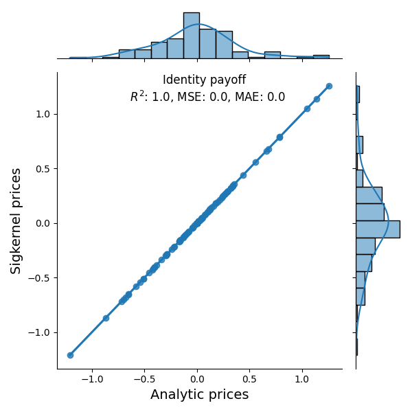
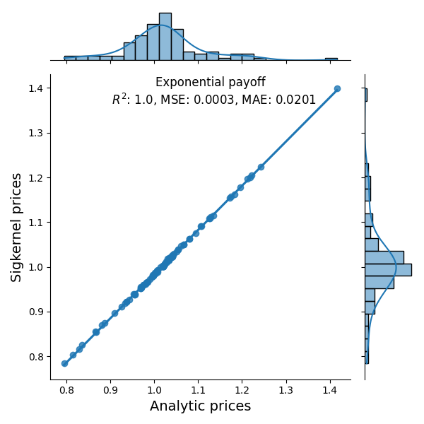
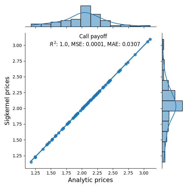
Figure 1. Analytic prices against Signature Kernel prices with $400$ collocation points.

As it can be observed from Figure 1, our kernel approach is capable to recovering with a high level of accuracy the prices for all considered payoff profiles.

5.2. Rough Bergomi

In this section, we make use of the following formulation of the rough Bergomi model introduced by [6] and already written down in the introduction

$$X_{t}:=\int_{0}^{t}\sqrt{\psi_{u}(\widehat{W}^{H}_{u})}\mathrm{d}B_{u}-\frac{1}{2}\int_{0}^{t}\psi_{u}(\widehat{W}^{H}_{u})\mathrm{d}u,\quad B_{u}:=\rho W_{u}^{1}+\sqrt{1-\rho^{2}}W_{u}^{2},$$

$$\psi_{t}(x):=\xi\exp\left\{\eta x-\frac{\eta^{2}}{2}t^{2H}\right\},\quad\widehat{W}^{H}_{t}:=\sqrt{2H}\int_{0}^{t}(t-u)^{H-\frac{1}{2}}\mathrm{d}W^{1}_{u},$$

for independent Brownian motions $(W^{1},W^{2})$. The hybrid scheme of [8] is used for efficient, $\mathcal{O}(\ell\log\ell)$, simulation of the Volterra process, $Y_{t}^{a}$, where $\ell$ is the length of the simulated paths. For the experiments we take the same parameters as in the repository, namely $T=1$, $\xi=0.055$, $\eta=1.9$, $\rho=-0.9$. We set the ground truth to be the Monte Carlo prices obtained with $100000$ sample paths.

(5.1) $$\partial_{t}u+\frac{1}{2}\psi_{t}(\gamma)(\partial_{xx}^{2}-\partial_{x})u+\frac{1}{2}\langle\partial_{\gamma\gamma}^{2}u,(K^{t},K^{t})\rangle+\rho\sqrt{\psi_{t}(\gamma)}\langle\partial_{\gamma}(\partial_{x}u),K^{t}\rangle=0,$$

To evaluate the conditional expectation in the Monte Carlo benchmark we remark that, setting

$$I^{t}_{s}:=\int_{t}^{s}K(s,r)\,\mathrm{d}W_{r},\quad\text{where }K(s,r)=\sqrt{2H}(s-r)^{H-\frac{1}{2}}$$

if $s>t$ and $0$ otherwise, the conditional expectation reduces to the following unconditional expectation as we showed in the introduction

(5.2) $$u(t,x,\omega)=\mathbb{E}\left[f\left(x+\int_{t}^{T}\sqrt{\psi_{s}(\omega_{s}+I^{t}_{s})}\,\mathrm{d}B_{s}-\frac{1}{2}\int_{t}^{T}\psi_{s}(\omega_{s}+I^{t}_{s})\,\mathrm{d}s\right)\right]$$

since $\Theta^{t}$ is an $\mathcal{F}_{t}$ measurable process and $I^{t}$ is independent from $\mathcal{F}_{t}$. Collocation points for the kernel method were sampled uniformly at random on $[0,1]$ for the time variable, uniformly at random on $[x_{min},x_{max}]$ for the price variables, where $x_{min},x_{max}$ were chosen using ground truth prices, and sampled from the process $\Theta^{t}$ for the path variable.

$H=0.1$ – Strike $=0.1$

Model	Monte Carlo			SigPPDE
Complexity	20 paths	100 paths	500 paths	20 c. pts	100 c. pts	500 c. pts
MSE	0.2070	0.0079	0.0080	0.2084	0.0016	0.0012
MAE	1.3193	0.2683	0.2300	0.6375	0.0714	0.0672

$H=0.1$ – Strike $=1.0$

Model	Monte Carlo			SigPPDE
Complexity	20 paths	100 paths	500 paths	20 c. pts	100 c. pts	500 c. pts
MSE	0.0324	0.0013	0.0001	0.1576	0.0092	0.0008
MAE	0.0679	0.0557	0.0131	0.7998	0.2671	0.0938

$H=0.3$ – Strike $=0.1$

Model	Monte Carlo			SigPPDE
Complexity	20 paths	100 paths	500 paths	20 c. pts	100 c. pts	500 c. pts
MSE	0.0198	0.0013	0.0005	0.1198	0.0026	0.0002
MAE	0.3330	0.0718	0.0624	0.6344	0.0973	0.0284

$H=0.3$ – Strike $=1.0$

Model	Monte Carlo			SigPPDE
Complexity	20 paths	100 paths	500 paths	20 c. pts	100 c. pts	500 c. pts
MSE	0.0113	0.0015	0.0006	0.4201	0.0046	0.0014
MAE	0.2341	0.0945	0.0679	1.1832	0.1050	0.0905

We consider two values of $H=0.1$ and $H=0.3$ and two strike values $K=0.1$ and $K=1.0$. We take the same number of sample paths and collocation points for Monte Carlo and the signature kernel solver respectively, and consider three different increasing values, namely $20$, $100$ and $500$. As it can be observed from the tables, the numerical performance in terms of MSE and MAE of the two algorithms are comparable across the different settings.

The time complexity of a Monte Carlo scheme scales roughly as $\mathcal{O}(h^{-2}Nd^{2})$, where $N$ is the number of sample paths, $h$ is the discretisation step and $d$ is the dimension of the process. This complexity can further reduced to $\mathcal{O}((h\log(h))^{-1}Nd^{2})$ using schemes such as the one proposed by [8]. The complexity for evaluating our solver (once it has been trained offline) scales as $\mathcal{O}(h^{-2}\hat{N}d^{2})$ where $\hat{N}$ is the number of collocation points. This cost can be further reduced $\mathcal{O}(h^{-1}\hat{N}d^{2})$ if the operations are carried out on a GPU, see [44] for additional details. It is clear that a transparent comparison of complexities between our approach and Monte Carlo for pricing under rough volatility can only be achieved by obtaining error rates for the convergence of the approximations governing the values of $N$ and $\hat{N}$ respectively in the above complexities, which we intend to explore as future work.

Nevertheless, the PDE approach provides by design advantages over Monte Carlo methods. Indeedn, finite-dimension greeks are prone to instability, let alone pathwise ones, while all derivatives of the PPDE solution appear from (the linear combination of) standard PDEs.

5.3. Comparison with neural PDE solvers

As antiticipated, we will conclude this section with some remarks aimed at comparing our kernel approach to the numerous neural network techniques to solve PPDE which have been proposed in the literature in recent years. Neural PDE solvers such as DGM [49] and PINNs [41] essentially parameterise the solution of the PDE as a neural network which is then trained using the PDE and its boundary conditions as loss function. One drawback of these approaches in the path-dependent setting [43, 48, 31] is that they require a time-discretisation of the solution. The time grids over which solutions and derivatives are evaluated during training and testing need to agree, usually followed by an arbitrary interpolation. On the contrary, our kernel approach operates directly on continuous paths, and it is therefore mesh-free. Furthermore, derivatives can be accessed directly by differentiating kernels, with no need to prematurely discretise in time. We note that concomitant to this paper is [23], which uses a neural rough differential equation (Neural RDE) model [39, 46] to parameterise the solution of a PPDE and is therefore also mesh-free. Another drawback of neural PDE solvers is that their theoretical analysis is often limited to density/universal approximation results; showing the existence of a network of a requisite size achieving a certain error rate, without guarantees whether this network is computable in practice. In fact the optimisation, done with variants of stochastic gradient descent, is never convex so there is no guarantee to attain a global minimum. Our kernel approach boils down to a convex finite dimensional optimisation, guaranteed to attain the unique global minimum, and that is consistent with the original problem when the number of collocation points is sent to infinity.

6. Outlook

The numerical solver presented in this paper competes with Monte Carlo methods in terms of the balance between complexity and accuracy. Our next objective will be to derive error estimates for the proposed method with respect to the number of collocation points in order to carry out a fair comparison. This step is essential for choosing the collocation points in an optimal way and better assess the efficiency of the algorithm. For this purpose we may follow the approach of [5] or decide to regularise our optimisation problem as in [15]. Further extensions include PPDEs arising from general Volterra processes, non-linear PPDEs, and path-dependent payoffs as the VIX example presented in Subsection 2.3.2. Finally, the inverse problem is particularly relevant for financial applications. We expect that the calibration of model parameters can be considerably sped up if the kernel is enhanced with this additional data.

Appendix A Proofs of signature and signature kernel estimates

A.1. Differentiability and continuity estimates for the signature

For the sake of uncluttering notations, in this section we fix $t\in\mathbb{T}$ and we will write $\left\lvert\gamma\right\rvert_{1}$ instead of $\left\lvert\gamma\right\rvert_{1-var;[t,T]}$ and $\left\lVert\gamma\right\rVert_{0}$ instead of $\left\lVert\gamma\right\rVert_{0;[t,T]}$ for every $\gamma\in\mathrm{BV}_{t}$. We present estimates for the signature and its derivatives, in passing obtaining CDEs satisfied by the latter, and showing continuity with respect to the $C^{0}$-norm as claimed in Proposition 3.14. The following lemma is inspired from Theorems 3.15 and 4.4 from [25].

Lemma A.1.

Let Assumption 3.10 hold for $g$. For all $\gamma,\bar{\gamma},\eta,{\bar{\eta}}\in\mathrm{BV}_{t}$, the signature is two times differentiable. Morever, there exist continuous functions $\overline{S_{k}}:\mathbb{R}_{+}^{k}\to\mathbb{R}_{+}$ and $\overline{DS_{k}}:\mathbb{R}_{+}^{k}\to\mathbb{R}_{+}$, for $k=1,2,3$, such that the following estimates hold

(A.1) $$\sup_{t^{\prime}\in[t,T]}\left\lVert S(\gamma^{g})_{t^{\prime}}\right\rVert_{\overline{T(\mathcal{H}_{g})}}\leq\overline{S_{0}}(\left\lvert\gamma\right\rvert_{1});$$

(A.2) $$\sup_{t^{\prime}\in[t,T]}\left\lVert S(\gamma^{g})_{t^{\prime}}-S(\bar{\gamma}^{g})_{t^{\prime}}\right\rVert_{\overline{T(\mathcal{H}_{g})}}\leq\left\lVert\gamma-\bar{\gamma}\right\rVert_{0}\overline{DS_{0}}(\left\lvert\gamma\right\rvert_{1},\left\lvert\bar{\gamma}\right\rvert_{1});$$

(A.3) $$\sup_{t^{\prime}\in[t,T]}\left\lVert\partial^{\eta}_{\gamma}S(\gamma^{g})_{t^{\prime}}\right\rVert_{\overline{T(\mathcal{H}_{g})}}\leq\overline{S_{1}}(\left\lvert\gamma\right\rvert_{1},\left\lVert\eta\right\rVert_{1});$$

(A.4) $$\sup_{t^{\prime}\in[t,T]}\left\lVert\partial^{\eta}_{\gamma}S(\gamma^{g})_{t^{\prime}}-\partial^{\eta}_{\gamma}S(\bar{\gamma}^{g})_{t^{\prime}}\right\rVert_{\overline{T(\mathcal{H}_{g})}}\leq\left\lVert\gamma-\bar{\gamma}\right\rVert_{0}\overline{DS_{1}}(\left\lvert\gamma\right\rvert_{1},\left\lvert\bar{\gamma}\right\rvert_{1},\left\lVert\eta\right\rVert_{1});$$

(A.5) $$\sup_{t^{\prime}\in[t,T]}\left\lVert\partial^{\eta{\bar{\eta}}}_{\gamma}S(\gamma^{g})_{t^{\prime}}\right\rVert_{\overline{T(\mathcal{H}_{g})}}\leq\overline{S_{2}}(\left\lvert\gamma\right\rvert_{1},\left\lVert\eta\right\rVert_{1},\left\lVert{\bar{\eta}}\right\rVert_{1});$$

(A.6) $$\sup_{t^{\prime}\in[t,T]}\left\lVert\partial^{\eta{\bar{\eta}}}_{\gamma}S(\gamma^{g})_{t^{\prime}}-\partial^{\eta{\bar{\eta}}}_{\gamma}S(\bar{\gamma}^{g})_{t^{\prime}}\right\rVert_{\overline{T(\mathcal{H}_{g})}}\leq\left\lVert\gamma-\bar{\gamma}\right\rVert_{0}\overline{DS_{2}}(\left\lvert\gamma\right\rvert_{1},\left\lvert\bar{\gamma}\right\rvert_{1},\left\lVert\eta\right\rVert_{1},\left\lVert{\bar{\eta}}\right\rVert_{1}).$$

Proof.

Let $0\leq t\leq t^{\prime}\leq T$ and $\gamma,\bar{\gamma},\eta,{\bar{\eta}}\in\mathrm{BV}_{t}$.

1) The signature satisfies

$$S(\gamma^{g})_{t^{\prime}}=\bm{1}+\int_{t}^{t^{\prime}}S(\gamma)_{u}\cdot\,\mathrm{d}\gamma_{u}^{g}=\bm{1}+\int_{t}^{t^{\prime}}S(\gamma)_{u}\cdot\nabla g(\gamma_{u},\cdot)\,\mathrm{d}\gamma_{u},$$

hence we have the bound

(A.7) $$\left\lVert S(\gamma^{g})_{t^{\prime}}\right\rVert_{\overline{T(\mathcal{H}_{g})}} \leq\bm{1}+\int_{t}^{t^{\prime}}\left\lVert S(\gamma)_{u}\right\rVert_{\overline{T(\mathcal{H}_{g})}}\cdot\left\lVert\nabla g(\gamma_{u},\cdot)\,\mathrm{d}\gamma_{u}\right\rVert_{\overline{T(\mathcal{H}_{g})}}$$

$$\leq\bm{1}+\int_{t}^{t^{\prime}}\left\lVert S(\gamma)_{u}\right\rVert_{\overline{T(\mathcal{H}_{g})}}\left\lVert\nabla g(\gamma_{u},\cdot)\right\rVert_{\mathcal{H}_{g}}\left\lvert\,\mathrm{d}\gamma_{u}\right\rvert,$$

where $\left\lVert\nabla g(\gamma_{u},\cdot)\right\rVert_{\mathcal{H}_{g}}=\sum_{i,j=1}^{e}\partial^{2}_{x^{i}y^{j}}g(\gamma_{u},\gamma_{u})\leq\overline{g_{11}}$ and $\left\lvert\,\mathrm{d}\gamma_{u}\right\rvert=\left\lvert\dot{\gamma}_{u}\right\rvert\,\mathrm{d}u$. By Grönwall’s lemma [25, Lemma 3.2] this yields

$$\sup_{t^{\prime}\in[t,T]}\left\lVert S(\gamma^{g})_{t^{\prime}}\right\rVert_{\overline{T(\mathcal{H}_{g})}}\leq\mathrm{e}^{\overline{g_{11}}\left\lvert\gamma\right\rvert_{1}}=:\overline{S_{0}}(\gamma).$$

2) Furthermore, [25, Proposition 2.9] gives the $1$-variation bound

$$\left\lvert\left\lVert S(\gamma^{g})_{\cdot}\right\rVert_{\overline{T(\mathcal{H}_{g})}}\right\rvert_{1}\leq\overline{S_{0}}(\gamma)\overline{g_{11}}\left\lvert\gamma\right\rvert_{1}.$$

For any $\bar{\gamma}\in\mathrm{BV}_{t}$, imitating the proof of [25, Theorem 3.15] yields

$$\left\lVert S(\gamma^{g})_{t^{\prime}}-S(\bar{\gamma}^{g})_{t^{\prime}}\right\rVert_{\overline{T(\mathcal{H}_{g})}} \leq\int_{t}^{t^{\prime}}\left\lVert S(\gamma^{g})_{u}-S(\bar{\gamma}^{g})_{u}\right\rVert_{\overline{T(\mathcal{H}_{g})}}\left\lvert\,\mathrm{d}\gamma^{g}_{u}\right\rvert+\left\lVert\int_{t}^{t^{\prime}}S(\bar{\gamma}^{g})\,\mathrm{d}(\gamma^{g}-\bar{\gamma}^{g})_{u}\right\rVert_{\overline{T(\mathcal{H}_{g})}}$$

$$\leq\int_{t}^{t^{\prime}}\left\lVert S(\gamma^{g})_{u}-S(\bar{\gamma}^{g})_{u}\right\rVert_{\overline{T(\mathcal{H}_{g})}}\overline{g_{11}}\left\lvert\,\mathrm{d}\gamma_{u}\right\rvert+\left\lVert\left\lVert\gamma^{g}-\bar{\gamma}^{g}\right\rVert_{\mathcal{H}_{g}}\right\rVert_{0}\big{(}1+\left\lvert\left\lVert S(\bar{\gamma}^{g})_{\cdot}\right\rVert_{\overline{T(\mathcal{H}_{g})}}\right\rvert_{1}\big{)}$$

Thus, applying the inequality $\left\lVert\left\lVert\gamma^{g}-\bar{\gamma}^{g}\right\rVert_{\mathcal{H}_{g}}\right\rVert_{0}\leq\overline{g_{11}}\left\lVert\gamma-\bar{\gamma}\right\rVert_{0}$ and Grönwall’s lemma we obtain

$$\sup_{t^{\prime}\in[t,T]}\left\lVert S(\gamma^{g})_{t^{\prime}}-S(\bar{\gamma}^{g})_{t^{\prime}}\right\rVert_{\overline{T(\mathcal{H}_{g})}}\leq\left\lVert\gamma-\bar{\gamma}\right\rVert_{0}\big{(}1+\overline{S_{0}}(\bar{\gamma})\overline{g_{11}}\left\lvert\bar{\gamma}\right\rvert_{1}\big{)}\mathrm{e}^{\overline{g_{11}}\left\lvert\gamma\right\rvert_{1}}=:\left\lVert\gamma-\bar{\gamma}\right\rVert_{0}\overline{DS_{0}}(\left\lvert\gamma\right\rvert_{1},\left\lvert\bar{\gamma}\right\rvert_{1}),$$

where $\overline{DS_{0}}:\mathbb{R}^{2}\to\mathbb{R}$ is a continuous function.

3) We start with the following observation. For all $u\in[t,T]$ we have

$$\lim_{\varepsilon\to 0}\frac{1}{\varepsilon}\,\mathrm{d}(\gamma+\varepsilon\eta)^{g}_{u}-\gamma^{g}_{u}) =\lim_{\varepsilon\to 0}\frac{1}{\varepsilon}\sum_{i=1}^{e}\Big{\{}\partial_{i}g(\gamma_{u}+\varepsilon\eta_{u},\cdot)\,\mathrm{d}(\gamma_{u}^{i}+\varepsilon\eta_{u}^{i})-\partial_{i}g(\gamma_{u},\cdot)\,\mathrm{d}\gamma_{u}^{i}\Big{\}}$$

$$=\lim_{\varepsilon\to 0}\frac{1}{\varepsilon}\sum_{i=1}^{e}\big{\{}\partial_{i}g(\gamma_{u}+\varepsilon\eta_{u},\cdot)-\partial_{i}g(\gamma_{u},\cdot)\big{\}}\,\mathrm{d}\gamma_{u}^{i}+\lim_{\varepsilon\to 0}\sum_{i=1}^{e}\partial_{i}g(\gamma_{u}+\varepsilon\eta_{u},\cdot)\,\mathrm{d}\eta^{i}_{u}$$

$$=\sum_{i=1}^{e}\bigg{\{}\partial^{\eta}_{\gamma}\partial_{x^{i}}g(\gamma_{u},\cdot)\,\mathrm{d}\gamma^{i}_{u}+\partial_{x^{i}}g(\gamma_{u},\cdot)\,\mathrm{d}\eta_{u}^{i}\bigg{\}}$$

$$=\,\mathrm{d}\left\{\sum_{i=1}^{e}\partial_{x^{i}}g(\gamma_{u},\cdot)\eta^{i}_{u}\right\}$$

(A.8) $$=\,\mathrm{d}\Big{\{}\partial^{\eta}_{\gamma}G(\gamma)_{u}\Big{\}}$$

Further, we note that, for all $\varepsilon>0$,

$$\frac{1}{\varepsilon}\sup_{t^{\prime}\in[t,T]}\left\lVert S(\gamma^{g})_{t^{\prime}}-S((\gamma+\varepsilon\eta)^{g})_{t^{\prime}}\right\rVert_{\overline{T(\mathcal{H}_{g})}}\leq\left\lVert\eta\right\rVert_{0}\overline{DS_{0}}(\left\lvert\gamma\right\rvert_{1},\left\lvert\gamma\right\rvert_{1}+\left\lvert\eta\right\rvert_{1}).$$

Hence, by dominated convergence and (A.8), we get

$$\partial^{\eta}_{\gamma}S(\gamma^{g})_{t^{\prime}} =\lim_{\varepsilon\to 0}\frac{1}{\varepsilon}\big{(}S((\gamma+\varepsilon\eta)^{g})_{t^{\prime}}-S(\gamma^{g})_{t^{\prime}}\big{)}$$

$$=\int_{t}^{t^{\prime}}\lim_{\varepsilon\to 0}\frac{1}{\varepsilon}\big{(}S((\gamma+\varepsilon\eta)^{g})_{u}-S(\gamma^{g})_{u}\big{)}\cdot\,\mathrm{d}\gamma_{u}^{g}+\int_{t}^{t^{\prime}}\lim_{\varepsilon\to 0}\frac{1}{\varepsilon}S(\gamma^{g})_{u}\cdot\,\mathrm{d}((\gamma+\varepsilon\eta)^{g})_{u}-\gamma^{g}_{u})$$

(A.9) $$=\int_{t}^{t^{\prime}}\partial^{\eta}_{\gamma}S(\gamma^{g})_{u}\cdot\,\mathrm{d}\gamma^{g}_{u}+\int_{t}^{t^{\prime}}S(\gamma^{g})_{u}\cdot\,\mathrm{d}\left\{\partial^{\eta}_{\gamma}G(\gamma)_{u}\right\}.$$

Note that $\left\lVert\partial_{x^{ij}}^{2}g(\gamma_{u},\cdot)\right\rVert_{\mathcal{H}_{g}}=\partial_{x^{ij}y^{ij}}^{4}g(\gamma_{u},\gamma_{u})$, and hence

$$\int_{t}^{t^{\prime}}\left\lVert\,\mathrm{d}\left\{\partial^{\eta}_{\gamma}G(\gamma)_{u}\right\}\right\rVert_{\mathcal{H}_{g}} \leq\int_{t}^{t^{\prime}}\sum_{i,j=1}^{e}\left\lVert\partial_{x^{ij}}g(\gamma_{u},\cdot)\right\rVert_{\mathcal{H}_{g}}\left\lvert\eta_{u}\right\rvert\left\lvert\,\mathrm{d}\gamma_{u}\right\rvert+\int_{t}^{t^{\prime}}\sum_{i=1}^{e}\left\lVert\partial_{x^{i}}g(\gamma_{u},\cdot)\right\rVert_{\mathcal{H}_{g}}\left\lvert\,\mathrm{d}\eta_{u}\right\rvert$$

(A.10) $$\leq\overline{g_{22}}\left\lVert\eta\right\rVert_{0}\left\lvert\gamma\right\rvert_{1}+\overline{g_{11}}\left\lvert\eta\right\rvert_{1}\leq\overline{G_{1}}(\left\lvert\gamma\right\rvert_{1},\left\lVert\eta\right\rVert_{1}),$$

where $\overline{G_{1}}:\mathbb{R}_{+}^{2}\to\mathbb{R}_{+}$ is a continuous function. Applying Grönwall’s lemma yields the estimate

$$\left\lVert\partial^{\eta}_{\gamma}S(\gamma^{g})_{t^{\prime}}\right\rVert_{\overline{T(\mathcal{H}_{g})}}\leq\overline{S_{0}}(\left\lvert\gamma\right\rvert_{1})\Big{(}\overline{g_{22}}\left\lVert\eta\right\rVert_{0}\left\lvert\gamma\right\rvert_{1}+\overline{g_{11}}\left\lvert\eta\right\rvert_{1}\Big{)}\mathrm{e}^{\overline{g_{11}}\left\lvert\gamma\right\rvert_{1}}=:\overline{S_{1}}(\left\lvert\gamma\right\rvert_{1},\left\lVert\eta\right\rVert_{1}).$$

4) Noting that, for all $t\leq s^{\prime}\leq t^{\prime}\leq T$,

$$\left\lvert\left\lVert\int_{t}^{\cdot}S(\gamma^{g})_{u}\cdot\,\mathrm{d}\left\{\partial^{\eta}_{\gamma}G(\gamma)_{u}\right\}\right\rVert_{\overline{T(\mathcal{H}_{g})}}\right\rvert_{1}\leq\overline{S_{0}}(\gamma)\left\lvert\int_{t}^{\cdot}\left\lVert\,\mathrm{d}\left\{\partial^{\eta}_{\gamma}G(\gamma)_{u}\right\}\right\rVert_{\mathcal{H}_{g}}\right\rvert_{1}\leq\overline{S_{0}}(\gamma)\overline{G_{1}}(\left\lvert\gamma\right\rvert_{1},\left\lVert\eta\right\rVert_{1}),$$

Proposition 2.9 of [25] thus gives

$$\left\lvert\left\lVert\partial^{\eta}_{\gamma}S(\gamma^{g})_{t^{\prime}}\right\rVert_{\overline{T(\mathcal{H}_{g})}}\right\rvert_{1}\leq\overline{S_{1}}(\left\lvert\gamma\right\rvert_{1},\left\lVert\eta\right\rVert_{1})\overline{g_{11}}\left\lvert\gamma\right\rvert_{1}+\overline{S_{0}}(\gamma)\overline{G_{1}}(\left\lvert\gamma\right\rvert_{1},\left\lVert\eta\right\rVert_{1}).$$

Then, from the integration by parts formula we observe that

$$\int_{t}^{t^{\prime}}\left\lvert\eta_{u}\right\rvert\,\mathrm{d}(\left\lvert\gamma_{u}-\bar{\gamma}_{u}\right\rvert)=\int_{t}^{t^{\prime}}\left\lvert\gamma_{u}-\bar{\gamma}_{u}\right\rvert\,\mathrm{d}\left\lvert\eta_{u}\right\rvert+\left\lvert\eta_{t}\right\rvert\left\lvert\gamma_{t}-\bar{\gamma}_{t}\right\rvert\leq\left\lVert\gamma-\bar{\gamma}\right\rVert_{0}\left\lvert\eta\right\rvert_{1}+\left\lVert\eta\right\rVert_{0}\left\lVert\gamma-\bar{\gamma}\right\rVert_{0}.$$

This allows us to study the following regularity:

$$\int_{t}^{t^{\prime}}\left\lVert\,\mathrm{d}\left\{\partial^{\eta}_{\gamma}(G(\gamma)_{u}-G(\bar{\gamma})_{u})\right\}\right\rVert_{\mathcal{H}_{g}}\leq\int_{t}^{t^{\prime}}\sum_{i,j=1}^{e}\left\lVert\partial_{x^{ij}}(g(\gamma_{u},\cdot)-g(\bar{\gamma}_{u},\cdot))\right\rVert_{\mathcal{H}_{g}}\left\lvert\eta_{u}\right\rvert\left\lvert\,\mathrm{d}\gamma_{u}\right\rvert$$

$$+\int_{t}^{t^{\prime}}\sum_{i,j=1}^{e}\left\lVert\partial_{x^{ij}}g(\bar{\gamma}_{u},\cdot)\right\rVert_{\mathcal{H}_{g}}\left\lvert\eta_{u}\right\rvert\left\lvert\,\mathrm{d}(\gamma_{u}-\bar{\gamma}_{u})\right\rvert+\int_{t}^{t^{\prime}}\sum_{i=1}^{e}\left\lVert\partial_{x^{i}}(g(\gamma_{u},\cdot)-g(\bar{\gamma}_{u},\cdot))\right\rVert_{\mathcal{H}_{g}}\left\lvert\,\mathrm{d}\eta_{u}\right\rvert$$

$$\leq\overline{g_{33}}\left\lVert\gamma-\bar{\gamma}\right\rVert_{0}\left\lVert\eta\right\rVert_{0}\left\lvert\gamma\right\rvert_{1}+\overline{g_{22}}\int_{t}^{t^{\prime}}\left\lvert\eta_{u}\right\rvert\,\mathrm{d}(\left\lvert\gamma_{u}-\bar{\gamma}_{u}\right\rvert)+\overline{g_{22}}\left\lVert\gamma-\bar{\gamma}\right\rVert_{0}\left\lvert\eta\right\rvert_{1}$$

$$\leq\left\lVert\gamma-\bar{\gamma}\right\rVert_{0}\overline{DG_{1}}(\left\lvert\gamma\right\rvert_{1},\left\lvert\bar{\gamma}\right\rvert_{1},\left\lVert\eta\right\rVert_{1}),$$

where $\overline{DG_{1}}:\mathbb{R}^{3}_{+}\to\mathbb{R}_{+}$ is a continuous function. We deduce that the difference of the source terms in (A.9) has the following bound

(A.11) $$\left\lVert\int_{t}^{t^{\prime}}S(\gamma^{g})_{u}\cdot\,\mathrm{d}\left\{\partial^{\eta}_{\gamma}G(\gamma)_{u}\right\}-\int_{t}^{t^{\prime}}S(\bar{\gamma}^{g})_{u}\cdot\,\mathrm{d}\left\{\partial^{\eta}_{\gamma}G(\bar{\gamma})_{u}\right\}\right\rVert_{\overline{T(\mathcal{H}_{g})}}$$

$$\leq\sup_{t^{\prime}\in[t,T]}\left\lVert S(\gamma^{g})_{t^{\prime}}-S(\bar{\gamma}^{g})_{t^{\prime}}\right\rVert_{\overline{T(\mathcal{H}_{g})}}\overline{G_{1}}(\gamma,\eta)+\sup_{t^{\prime}\in[t,T]}\left\lVert S(\gamma^{g})_{t^{\prime}}\right\rVert_{\overline{T(\mathcal{H}_{g})}}\int_{t}^{t^{\prime}}\left\lVert\,\mathrm{d}\left\{\partial^{\eta}_{\gamma}(G(\gamma)_{u}-G(\bar{\gamma})_{u})\right\}\right\rVert_{\mathcal{H}_{g}}$$

$$\leq\left\lVert\gamma-\bar{\gamma}\right\rVert_{0}\Big{(}\overline{DS_{0}}(\left\lvert\gamma\right\rvert_{1},\left\lvert\bar{\gamma}\right\rvert_{1})\overline{G_{1}}(\left\lvert\gamma\right\rvert_{1},\left\lVert\eta\right\rVert_{1})+\overline{S_{0}}(\gamma)\overline{DG_{1}}(\left\lvert\gamma\right\rvert_{1},\left\lvert\bar{\gamma}\right\rvert_{1},\left\lVert\eta\right\rVert_{1})\Big{)}.$$

In virtue of (A.9) and (A.11), the same arguments as in the proof of [25, Theorem 3.15] entails there exists a continuous function $\overline{DS_{1}}:\mathbb{R}^{3}_{+}\to\mathbb{R}_{+}$ such that

$$\sup_{t^{\prime}\in[t,T]} \left\lVert\partial^{\eta}_{\gamma}S(\gamma^{g})_{t^{\prime}}-\partial^{\eta}_{\gamma}S(\bar{\gamma}^{g})_{t^{\prime}}\right\rVert_{\overline{T(\mathcal{H}_{g})}}$$

$$\leq\mathrm{e}^{2\overline{g_{11}}(\left\lvert\gamma\right\rvert_{1}\vee\left\lvert\bar{\gamma}\right\rvert_{1})}\left\lVert\int_{t}^{t^{\prime}}S(\gamma^{g})_{u}\cdot\,\mathrm{d}\left\{\partial^{\eta}_{\gamma}G(\gamma)_{u}\right\}-\int_{t}^{t^{\prime}}S(\bar{\gamma}^{g})_{u}\cdot\,\mathrm{d}\left\{\partial^{\eta}_{\gamma}G(\bar{\gamma})_{u}\right\}\right\rVert_{\overline{T(\mathcal{H}_{g})}}$$

$$\leq\left\lVert\gamma-\bar{\gamma}\right\rVert_{0}\overline{DS_{1}}(\left\lvert\gamma\right\rvert_{1},\left\lvert\bar{\gamma}\right\rvert_{1},\left\lVert\eta\right\rVert_{1}).$$

5) The latest estimate allows to use dominated convergence one more time and compute the second derivative in the direction of $\eta,{\bar{\eta}}$:

(A.12) $$\partial^{\eta{\bar{\eta}}}_{\gamma}S(\gamma^{g})_{t^{\prime}} =\int_{t}^{t^{\prime}}\partial^{\eta{\bar{\eta}}}_{\gamma}S(\gamma^{g})_{u}\,\mathrm{d}\gamma^{g}_{u}+{\rm Source}(\gamma,\eta,{\bar{\eta}}),$$

where

$${\rm Source}(\gamma,\eta,{\bar{\eta}}):=\int_{t}^{t^{\prime}}\partial^{\eta}_{\gamma}S(\gamma^{g})_{u}\cdot\,\mathrm{d}\left\{\partial^{\bar{\eta}}_{\gamma}G(\gamma)_{u}\right\}+\int_{t}^{t^{\prime}}\partial^{\bar{\eta}}_{\gamma}S(\gamma^{g})_{u}\cdot\,\mathrm{d}\left\{\partial^{\eta}_{\gamma}G(\gamma)_{u}\right\}+\int_{t}^{t^{\prime}}S(\gamma^{g})_{u}\cdot\,\mathrm{d}\left\{\partial^{\eta{\bar{\eta}}}_{\gamma}G(\gamma)_{u}\right\}.$$

Using the same arguments as in (A.8) one deduces that

$$\int_{t}^{t^{\prime}}\left\lVert\,\mathrm{d}\left\{\partial^{\eta{\bar{\eta}}}_{\gamma}G(\gamma)_{u}\right\}\right\rVert_{\mathcal{H}_{g}} \leq\int_{t}^{t^{\prime}}\sum_{i,j,k=1}^{e}\left\lVert\partial^{3}_{x^{ijk}}g(\gamma_{u},\cdot)\right\rVert_{\mathcal{H}_{g}}\left\lvert{\bar{\eta}}_{u}\right\rvert\left\lvert\eta_{u}\right\rvert\left\lvert\,\mathrm{d}\gamma_{u}\right\rvert$$

$$\quad+\int_{t}^{t^{\prime}}\sum_{i,j=1}^{e}\left\lVert\partial^{2}_{x^{ij}}g(\gamma_{u},\cdot)\right\rVert_{\mathcal{H}_{g}}\Big{(}\left\lvert\eta_{u}\right\rvert\left\lvert\,\mathrm{d}{\bar{\eta}}_{u}\right\rvert+\left\lvert{\bar{\eta}}_{u}\right\rvert\left\lvert\,\mathrm{d}\eta_{u}\right\rvert\Big{)}$$

(A.13) $$\leq\overline{g_{33}}\left\lVert\eta\right\rVert_{0}\left\lVert{\bar{\eta}}\right\rVert_{0}\left\lvert\gamma\right\rvert_{1}+\overline{g_{22}}\Big{(}\left\lVert\eta\right\rVert_{0}\left\lvert{\bar{\eta}}\right\rvert_{1}+\left\lVert{\bar{\eta}}\right\rVert_{0}\left\lvert\eta\right\rvert_{1}\Big{)}\leq\overline{G_{2}}(\left\lvert\gamma\right\rvert_{1},\left\lVert\eta\right\rVert_{1},\left\lVert{\bar{\eta}}\right\rVert_{1}),$$

where $\overline{G_{2}}:\mathbb{R}_{+}^{3}\to\mathbb{R}_{+}$ is a continuous function. Grönwall’s inequality once again yields the bound

$$\sup_{t^{\prime}\in[t,T]}\left\lVert\partial^{\eta{\bar{\eta}}}_{\gamma}S(\gamma^{g})_{t^{\prime}}\right\rVert_{\overline{T(\mathcal{H}_{g})}}\leq\Big{(}\overline{S_{1}}(\gamma,\eta)\overline{G_{1}}(\gamma,{\bar{\eta}})+\overline{S_{1}}(\gamma,{\bar{\eta}})\overline{G_{1}}(\gamma,\eta)+\overline{S_{0}}(\gamma)\overline{G_{2}}(\gamma,\eta,{\bar{\eta}})\Big{)}\mathrm{e}^{\overline{g_{11}}\left\lvert\gamma\right\rvert_{1}}.$$

6) The same steps as for the first derivative yield the existence of a continuous function $\overline{DG_{2}}:\mathbb{R}^{4}\to\mathbb{R}$ such that

$$\int_{t}^{t^{\prime}}\left\lVert\,\mathrm{d}\left\{\partial^{\eta{\bar{\eta}}}_{\gamma}\big{(}G(\gamma)_{u}-G(\bar{\gamma})_{u}\big{)}\right\}\right\rVert_{\mathcal{H}_{g}}\leq\left\lVert\gamma-\bar{\gamma}\right\rVert_{0}\overline{DG_{2}}(\left\lvert\gamma\right\rvert_{1},\left\lvert\bar{\gamma}\right\rvert_{1},\left\lVert\eta\right\rVert_{1},\left\lVert{\bar{\eta}}\right\rVert_{1}).$$

Hence the difference of the source term for two paths $\gamma,\bar{\gamma}$ can be bounded as follows

$$\left\lVert{\rm Source}(\gamma,\eta,{\bar{\eta}})-{\rm Source}(\bar{\gamma},\eta,{\bar{\eta}})\right\rVert_{\overline{T(\mathcal{H}_{g})}}$$

$$\leq\left\lVert\gamma-\bar{\gamma}\right\rVert_{0}\Big{(}\overline{S_{1}}(\left\lvert\gamma\right\rvert_{1},\left\lVert\eta\right\rVert_{1})\overline{DG_{1}}(\left\lvert\gamma\right\rvert_{1},\left\lvert\bar{\gamma}\right\rvert_{1},\left\lVert\eta\right\rVert_{1})+\overline{G_{1}}(\left\lvert\gamma\right\rvert_{1},\left\lvert\bar{\gamma}\right\rvert_{1},\left\lVert\eta\right\rVert_{1})\overline{DS_{1}}(\left\lvert\gamma\right\rvert_{1},\left\lvert\bar{\gamma}\right\rvert_{1},\left\lVert\eta\right\rVert_{1})$$

$$\quad+\overline{S_{1}}(\left\lvert\gamma\right\rvert_{1},\left\lVert{\bar{\eta}}\right\rVert_{1})\overline{DG_{1}}(\left\lvert\gamma\right\rvert_{1},\left\lvert\bar{\gamma}\right\rvert_{1},\left\lVert{\bar{\eta}}\right\rVert_{1})+\overline{G_{1}}(\left\lvert\gamma\right\rvert_{1},\left\lvert\bar{\gamma}\right\rvert_{1},\left\lVert{\bar{\eta}}\right\rVert_{1})\overline{DS_{1}}(\left\lvert\gamma\right\rvert_{1},\left\lvert\bar{\gamma}\right\rvert_{1},\left\lVert{\bar{\eta}}\right\rVert_{1})$$

$$\quad+\overline{S_{0}}(\left\lvert\gamma\right\rvert_{1})\overline{G_{2}}(\left\lvert\gamma\right\rvert_{1},\left\lvert\bar{\gamma}\right\rvert_{1},\left\lVert\eta\right\rVert_{1},\left\lVert{\bar{\eta}}\right\rVert_{1})+\overline{DS_{0}}(\left\lvert\gamma\right\rvert_{1},\left\lvert\bar{\gamma}\right\rvert_{1})\overline{G_{2}}(\left\lvert\gamma\right\rvert_{1},\left\lvert\bar{\gamma}\right\rvert_{1},\left\lVert\eta\right\rVert_{1},\left\lVert{\bar{\eta}}\right\rVert_{1})\Big{)}.$$

Finally, by [25, Theorem 3.15] again there is a continuous function $\overline{DS_{2}}:\mathbb{R}^{4}\to\mathbb{R}$ such that

$$\sup_{t^{\prime}\in[t,T]}\left\lVert\partial^{\eta{\bar{\eta}}}_{\gamma}S(\gamma^{g})_{t^{\prime}}-\partial^{\eta{\bar{\eta}}}_{\gamma}S(\bar{\gamma}^{g})_{t^{\prime}}\right\rVert_{\overline{T(\mathcal{H}_{g})}}\leq\left\lVert\gamma-\bar{\gamma}\right\rVert_{0}\overline{DS_{2}}(\left\lvert\gamma\right\rvert_{1},\left\lvert\bar{\gamma}\right\rvert_{1},\left\lVert\eta\right\rVert_{1},\left\lVert{\bar{\eta}}\right\rVert_{1})$$

thus concluding the proof. ∎

A.2. Differentiability and continuity estimates for the signature kernel

We start by stating estimates for the signature kernel and its derivatives, which follow from Lemma A.1. The PDE formulations in Proposition 3.11 are immediate corollaries. In terms of notations, for two paths $\gamma\in\mathrm{BV}_{t}$ and $\tau\in\mathrm{BV}_{s}$, we will denote $\left\lvert\gamma\right\rvert_{1}=\left\lvert\gamma\right\rvert_{1-var;[t,T]}$ and $\left\lvert\tau\right\rvert_{1}=\left\lvert\tau\right\rvert_{1-var;[s,T]}$.

Lemma A.2.

Let Assumption and 3.10 hold for $g$. Let $s,t\in\mathbb{T}$, the paths $\gamma,\eta,{\bar{\eta}}\in\mathrm{BV}_{t}$ and $\tau\in\mathrm{BV}_{s}$. Then the following estimates hold:

$$\sup_{s^{\prime}\in[s,T],t^{\prime}\in[t,T]}\left\lvert\kappa^{g}(\gamma,\tau)_{s^{\prime},t^{\prime}}\right\rvert\leq\overline{S_{0}}(\left\lvert\gamma\right\rvert_{1})\overline{S_{0}}(\left\lvert\tau\right\rvert_{1});$$

$$\sup_{s^{\prime}\in[s,T],t^{\prime}\in[t,T]}\left\lvert\partial^{\eta}_{\gamma}\kappa^{g}(\gamma,\tau)_{s^{\prime},t^{\prime}}\right\rvert\leq\overline{S_{1}}(\left\lvert\gamma\right\rvert_{1},\left\lVert\eta\right\rVert_{1})\overline{S_{0}}(\left\lvert\tau\right\rvert_{1});$$

$$\sup_{s^{\prime}\in[s,T],t^{\prime}\in[t,T]}\left\lvert\partial^{\eta{\bar{\eta}}}_{\gamma}\kappa^{g}(\gamma,\tau)_{s^{\prime},t^{\prime}}\right\rvert\leq\overline{S_{2}}(\left\lvert\gamma\right\rvert_{1},\left\lVert\eta\right\rVert_{1},\left\lVert{\bar{\eta}}\right\rVert_{1})\overline{S_{0}}(\left\lvert\tau\right\rvert_{1}).$$

Proof.

Let $0\leq s\leq s^{\prime}\leq T$, $0\leq t\leq t^{\prime}\leq T$ and $\gamma,\eta,{\bar{\eta}}\in\mathrm{BV}_{t},\tau\in\mathrm{BV}_{s}$. By the definition of the signature kernel, Cauchy-Schwarz inequality and (A.1) we have

$$\left\lvert\kappa^{g}(\gamma,\tau)_{s^{\prime},t^{\prime}}\right\rvert=\left\lvert\langle S(\gamma^{g})_{t^{\prime}},S(\tau^{g})_{s^{\prime}}\rangle\right\rvert\leq\left\lVert S(\gamma^{g})_{t^{\prime}}\right\rVert_{\overline{T(\mathcal{H}_{g})}}\left\lVert S(\tau^{g})_{s^{\prime}}\right\rVert_{\overline{T(\mathcal{H}_{g})}}\leq\overline{S_{0}}(\left\lvert\gamma\right\rvert_{1})\overline{S_{0}}(\left\lvert\tau\right\rvert_{1}).$$

Then for any $\varepsilon>0$, Cauchy-Schwarz inequality and (A.2) yield

$$\left\lvert\kappa^{g}(\gamma+\varepsilon\eta,\tau)_{s^{\prime},t^{\prime}}-\kappa^{g}(\gamma,\tau)_{s^{\prime},t^{\prime}}\right\rvert\leq\left\lVert\eta\right\rVert_{0}\overline{DS_{0}}(\left\lvert\gamma\right\rvert_{1},\left\lvert\gamma\right\rvert_{1}+\left\lvert\eta\right\rvert_{1})\overline{S_{0}}(\left\lvert\tau\right\rvert_{1}).$$

Therefore, dominated convergence, Cauchy-Schwarz and (A.3) entail

$$\left\lvert\partial_{\gamma}^{\eta}\kappa^{g}(\gamma,\tau)_{s^{\prime},t^{\prime}}\right\rvert=\left\lvert\langle\partial^{\gamma}_{\eta}S(\gamma^{g})_{t^{\prime}},S(\tau^{g})_{s^{\prime}}\rangle\right\rvert\leq\overline{S_{1}}(\left\lvert\gamma\right\rvert_{1},\left\lVert\eta\right\rVert_{1})\overline{S_{0}}(\left\lvert\tau\right\rvert_{1}).$$

The same ideas coupled with the bounds (A.5) and (A.6) lead to the last estimate. ∎

Proof of Proposition 3.11.

Let $0\leq s\leq s^{\prime}\leq T$ and $0\leq t\leq t^{\prime}\leq T$ and $\gamma,\eta,{\bar{\eta}}\in\mathrm{BV}_{t},\tau\in\mathrm{BV}_{s}$.

1) In virtue of (A.2), dominated convergence allows to push the limit inside the integrals:

$$\partial_{\gamma}^{\eta}\kappa^{g}(\gamma,\tau)_{s^{\prime},t^{\prime}} =\lim_{\varepsilon\to 0}\frac{1}{\varepsilon}\left(\kappa^{g}(\gamma+\varepsilon\eta,\tau)_{s^{\prime},t^{\prime}}-\kappa^{g}(\gamma,\tau)_{s^{\prime},t^{\prime}}\right)$$

$$=\lim_{\varepsilon\to 0}\frac{1}{\varepsilon}\int_{s}^{s^{\prime}}\int_{t}^{t^{\prime}}\left(\kappa^{g}(\gamma+\varepsilon\eta,\tau)_{u,v}\left\langle\,\mathrm{d}(\gamma+\varepsilon\eta)^{g}_{u},\,\mathrm{d}\tau^{g}_{v}\right\rangle_{\mathcal{H}_{g}}-\kappa^{g}(\gamma,\tau)_{u,v}\left\langle\,\mathrm{d}\gamma^{g}_{u},\,\mathrm{d}\tau^{g}_{v}\right\rangle_{\mathcal{H}_{g}}\right)$$

$$=\int_{s}^{s^{\prime}}\int_{t}^{t^{\prime}}\lim_{\varepsilon\to 0}\frac{1}{\varepsilon}\Big{(}\kappa^{g}(\gamma+\varepsilon\eta,\tau)_{u,v}-\kappa^{g}(\gamma,\tau)_{u,v}\Big{)}\left\langle\,\mathrm{d}(\gamma+\varepsilon\eta)^{g}_{u},\,\mathrm{d}\tau^{g}_{v}\right\rangle_{\mathcal{H}_{g}}$$

$$\qquad+\kappa^{g}(\gamma,\tau)_{u,v}\lim_{\varepsilon\to 0}\frac{1}{\varepsilon}\left\langle\,\mathrm{d}(\gamma+\varepsilon\eta)^{g}_{u}-\,\mathrm{d}\gamma^{g}_{u},\,\mathrm{d}\tau^{g}_{v}\right\rangle_{\mathcal{H}_{g}}$$

$$=\int_{s}^{s^{\prime}}\int_{t}^{t^{\prime}}\left(\partial_{\gamma}^{\eta}\kappa^{g}(\gamma,\tau)_{u,v}\left\langle\,\mathrm{d}\gamma^{g}_{u},\,\mathrm{d}\tau^{g}_{v}\right\rangle_{\mathcal{H}_{g}}+\kappa^{g}(\gamma,\tau)_{u,v}\lim_{\varepsilon\to 0}\frac{1}{\varepsilon}\left\langle\,\mathrm{d}(\gamma+\varepsilon\eta)^{g}_{u}-\,\mathrm{d}\gamma^{g}_{u},\,\mathrm{d}\tau^{g}_{v}\right\rangle_{\mathcal{H}_{g}}\right).$$

For all $u\in[t,T]$ and $v\in[s,T]$ we have

$$\lim_{\varepsilon\to 0}\frac{1}{\varepsilon}\Big{\langle}\,\mathrm{d}(\gamma+\varepsilon\eta)^{g}_{u}-\gamma^{g}_{u},\,\mathrm{d}\tau^{g}_{v}\Big{\rangle}_{\mathcal{H}_{g}}$$

$$=\lim_{\varepsilon\to 0}\frac{1}{\varepsilon}\sum_{i,k=1}^{e}\Big{\langle}\partial_{i}g(\gamma_{u}+\varepsilon\eta_{u},\cdot)\,\mathrm{d}(\gamma_{u}^{i}+\varepsilon\eta_{u}^{i})-\partial_{i}g(\gamma_{u},\cdot)\,\mathrm{d}\gamma_{u}^{i},\partial_{k}g(\tau_{v},\cdot)\,\mathrm{d}\tau^{k}_{v}\Big{\rangle}$$

$$=\lim_{\varepsilon\to 0}\frac{1}{\varepsilon}\sum_{i,k=1}^{e}\Big{\langle}\partial_{i}g(\gamma_{u}+\varepsilon\eta_{u},\cdot)-\partial_{i}g(\gamma_{u},\cdot),\partial_{k}g(\tau_{v},\cdot)\Big{\rangle}\,\mathrm{d}\gamma_{u}^{i}\,\mathrm{d}\tau^{k}_{v}+\lim_{\varepsilon\to 0}\sum_{i,k=1}^{e}\Big{\langle}\partial_{i}g(\gamma_{u}+\varepsilon\eta_{u},\cdot),\partial_{k}g(\tau_{v},\cdot)\Big{\rangle}\,\mathrm{d}\eta^{i}_{u}\,\mathrm{d}\tau^{k}_{v}$$

$$=\sum_{i,k=1}^{e}\lim_{\varepsilon\to 0}\bigg{\{}\frac{1}{\varepsilon}\partial_{x^{i}}\partial_{y^{k}}\Big{(}g(\gamma_{u}+\varepsilon\eta_{u},\tau_{v})-g(\gamma_{u},\tau_{v})\Big{)}\,\mathrm{d}\gamma_{u}^{i}\,\mathrm{d}\tau^{k}_{v}+\partial_{x^{i}}\partial_{y^{k}}g(\gamma_{u}+\varepsilon\eta_{u},\tau_{v})\,\mathrm{d}\eta^{i}_{u}\,\mathrm{d}\tau^{k}_{v}\bigg{\}}$$

$$=\sum_{i,k=1}^{e}\bigg{\{}\partial^{\eta}_{\gamma}\partial_{x^{i}y^{k}}^{2}g(\gamma_{u},\tau_{v})\,\mathrm{d}\gamma^{i}_{u}+\partial_{x^{i}y^{k}}^{2}g(\gamma_{u},\tau_{v})\,\mathrm{d}\eta_{u}^{i}\bigg{\}}\,\mathrm{d}\tau^{k}_{v}$$

(A.14) $$=\sum_{i,k=1}^{e}\bigg{\{}\sum_{j=1}^{e}\partial_{x^{ij}y^{k}}^{3}g(\gamma_{u},\tau_{v})\eta_{u}^{j}\,\mathrm{d}\gamma_{u}^{i}+\partial_{x^{i}y^{k}}^{2}g(\gamma_{u},\tau_{v})\,\mathrm{d}\eta_{u}^{i}\bigg{\}}\,\mathrm{d}\tau^{k}_{v}$$

where we used the reproducing property of derivatives of $g$ (3.13) and we can swap partial derivatives because $g(\cdot,x)\in C^{2}(V,\mathbb{R})$ for all $x\in V$. Unrolling in the other direction one can also obtain

$$\sum_{i,k=1}^{e}\bigg{\{}\sum_{j=1}^{e}\partial_{x^{ij}y^{k}}^{3}g(\gamma_{u},\tau_{v})\eta_{u}^{j}\,\mathrm{d}\gamma_{u}^{i}+\partial_{x^{i}y^{k}}^{2}g(\gamma_{u},\tau_{v})\,\mathrm{d}\eta_{u}^{i}\bigg{\}}\,\mathrm{d}\tau^{k}_{v} =\left\langle\,\mathrm{d}\left\{\sum_{i=1}^{e}\partial_{x^{i}}g(\gamma_{u},\cdot)\eta^{i}_{u}\right\},\,\mathrm{d}\tau^{g}_{v}\right\rangle$$

(A.15) $$=\left\langle\,\mathrm{d}\Big{\{}\partial^{\eta}_{\gamma}G(\gamma)_{u}\Big{\}},\,\mathrm{d}\tau^{g}_{v}\right\rangle.$$

The expressions (A.15) and (A.14) yield (3.16) and (A.2) respectively.

2) We take the terms of (A.2) one by one to compute

$$\partial_{\gamma}^{\eta{\bar{\eta}}}\kappa^{g}(\gamma,\tau)_{s^{\prime},t^{\prime}} :=\lim_{\varepsilon\to 0}\frac{1}{\varepsilon}\Big{(}\partial_{\gamma}^{\eta}\kappa^{g}(\gamma+\varepsilon{\bar{\eta}},\tau)_{s^{\prime},t^{\prime}}-\partial_{\gamma}^{\eta}\kappa^{g}(\gamma,\tau)_{s^{\prime},t^{\prime}}\Big{)}$$

$$=\lim_{\varepsilon\to 0}\frac{1}{\varepsilon}\Bigg{\{}\int_{s}^{s^{\prime}}\int_{t}^{t^{\prime}}\partial_{\gamma}^{\eta}\kappa^{g}(\gamma+\varepsilon{\bar{\eta}},\tau)_{u,v}\sum_{i,k=1}^{e}\partial_{x^{i}y^{k}}^{2}g(\gamma_{u}+\varepsilon{\bar{\eta}}_{u},\tau_{v})\,\mathrm{d}(\gamma^{i}_{u}+\varepsilon{\bar{\eta}}^{i}_{u})\,\mathrm{d}\tau^{k}_{v}$$

$$\qquad\qquad\qquad-\int_{s}^{s^{\prime}}\int_{t}^{t^{\prime}}\partial_{\gamma}^{\eta}\kappa^{g}(\gamma,\tau)_{u,v}\sum_{i,k=1}^{e}\partial_{x^{i}y^{k}}^{2}g(\gamma_{u},\tau_{v})\,\mathrm{d}\gamma^{i}_{u}\,\mathrm{d}\tau^{k}_{v}\Bigg{\}}$$

$$+\lim_{\varepsilon\to 0}\frac{1}{\varepsilon}\Bigg{\{}\int_{s}^{s^{\prime}}\int_{t}^{t^{\prime}}\kappa^{g}(\gamma+\varepsilon{\bar{\eta}},\tau)_{u,v}\sum_{i,j,k=1}^{e}\partial_{x^{ij}y^{k}}^{3}g(\gamma_{u}+\varepsilon{\bar{\eta}}_{u},\tau_{v})\eta_{u}^{j}\,\mathrm{d}(\gamma_{u}^{i}+\varepsilon{\bar{\eta}}^{i}_{u})\,\mathrm{d}\tau^{k}_{v}$$

$$\qquad\qquad\qquad-\int_{s}^{s^{\prime}}\int_{t}^{t^{\prime}}\kappa^{g}(\gamma,\tau)_{u,v}\sum_{i,j,k=1}^{e}\partial_{x^{ij}y^{k}}^{3}g(\gamma_{u},\tau_{v})\eta_{u}^{j}\,\mathrm{d}\gamma_{u}^{i}\,\mathrm{d}\tau^{k}_{v}\Bigg{\}}$$

$$+\lim_{\varepsilon\to 0}\frac{1}{\varepsilon}\Bigg{\{}\int_{s}^{s^{\prime}}\int_{t}^{t^{\prime}}\kappa^{g}(\gamma+\varepsilon{\bar{\eta}},\tau)_{u,v}\sum_{i,k=1}^{e}\partial_{x^{i}y^{k}}^{2}g(\gamma_{u}+\varepsilon{\bar{\eta}}_{u},\tau_{v})\,\mathrm{d}\eta_{u}^{i}\,\mathrm{d}\tau^{k}_{v}$$

$$\qquad\qquad\qquad-\int_{s}^{s^{\prime}}\int_{t}^{t^{\prime}}\kappa^{g}(\gamma,\tau)_{u,v}\sum_{i,k=1}^{e}\partial_{x^{i}y^{k}}^{2}g(\gamma_{u},\tau_{v})\,\mathrm{d}\eta_{u}^{i}\,\mathrm{d}\tau^{k}_{v}\Bigg{\}}.$$

Thanks to Lemma A.1, we can use dominated convergence to swap limits and integrals. After rearranging terms we obtain

$$\partial_{\gamma}^{\eta{\bar{\eta}}}\kappa^{g}(\gamma,\tau)_{s^{\prime},t^{\prime}} =\int_{s}^{s^{\prime}}\int_{t}^{t^{\prime}}\partial_{\gamma}^{\eta{\bar{\eta}}}\kappa^{g}(\gamma,\tau)_{u,v}\sum_{i,k=1}^{e}\partial_{x^{i}y^{k}}^{2}g(\gamma_{u},\tau_{v})\,\mathrm{d}\gamma^{i}_{u}\,\mathrm{d}\tau^{k}_{v}$$

$$\quad+\int_{s}^{s^{\prime}}\int_{t}^{t^{\prime}}\partial_{\gamma}^{\eta}\kappa^{g}(\gamma,\tau)_{u,v}\sum_{i,k,l=1}^{e}\partial_{x^{il}y^{k}}^{3}g(\gamma_{u},\tau_{v}){\bar{\eta}}^{l}_{u}\,\mathrm{d}\gamma^{i}_{u}\,\mathrm{d}\tau^{k}_{v}$$

$$\quad+\int_{s}^{s^{\prime}}\int_{t}^{t^{\prime}}\partial_{\gamma}^{\eta}\kappa^{g}(\gamma,\tau)_{u,v}\sum_{i,k=1}^{e}\partial_{x^{i}y^{k}}^{2}g(\gamma_{u},\tau_{v})\,\mathrm{d}{\bar{\eta}}^{i}_{u}\,\mathrm{d}\tau^{k}_{v}$$

$$\quad+\int_{s}^{s^{\prime}}\int_{t}^{t^{\prime}}\partial^{{\bar{\eta}}}_{\gamma}\kappa^{g}(\gamma,\tau)_{u,v}\sum_{i,j,k=1}^{e}\partial_{x^{ij}y^{k}}^{3}g(\gamma_{u},\tau_{v})\eta_{u}^{j}\,\mathrm{d}\gamma_{u}^{i}\,\mathrm{d}\tau^{k}_{v}$$

$$\quad+\int_{s}^{s^{\prime}}\int_{t}^{t^{\prime}}\kappa^{g}(\gamma,\tau)_{u,v}\sum_{i,j,k,l=1}^{e}\partial_{x^{ijl}y^{k}}^{4}g(\gamma_{u},\tau_{v}){\bar{\eta}}^{l}_{u}\eta_{u}^{j}\,\mathrm{d}\gamma_{u}^{i}\,\mathrm{d}\tau^{k}_{v}$$

$$\quad+\int_{s}^{s^{\prime}}\int_{t}^{t^{\prime}}\kappa^{g}(\gamma,\tau)_{u,v}\sum_{i,j,k=1}^{e}\partial_{x^{ij}y^{k}}^{3}g(\gamma_{u},\tau_{v})\eta_{u}^{j}\,\mathrm{d}{\bar{\eta}}_{u}^{i}\,\mathrm{d}\tau^{k}_{v}$$

$$\quad+\int_{s}^{s^{\prime}}\int_{t}^{t^{\prime}}\partial^{{\bar{\eta}}}_{\gamma}\kappa^{g}(\gamma,\tau)_{u,v}\sum_{i,k=1}^{e}\partial_{x^{i}y^{k}}^{2}g(\gamma_{u},\tau_{v})\,\mathrm{d}\eta_{u}^{i}\,\mathrm{d}\tau^{k}_{v}$$

$$\quad+\int_{s}^{s^{\prime}}\int_{t}^{t^{\prime}}\kappa^{g}(\gamma,\tau)_{u,v}\sum_{i,k,l=1}^{e}\partial_{x^{il}y^{k}}^{3}g(\gamma_{u},\tau_{v}){\bar{\eta}}^{l}_{u}\,\mathrm{d}\eta_{u}^{i}\,\mathrm{d}\tau^{k}_{v}$$

where we also used the property (3.13). We can regroup the terms according to the order of $\kappa^{g}$, using $\sum_{i,k=1}^{e}\partial_{x^{i}y^{k}}^{2}g(\gamma_{u},\tau_{v})\,\mathrm{d}\gamma^{i}_{u}\,\mathrm{d}\tau^{k}_{v}=\langle\,\mathrm{d}\gamma^{g}_{u},\,\mathrm{d}\tau^{g}_{v}\rangle_{\mathcal{H}_{g}}$, Equation (A.15) and similarly for the next order:

(A.16) $$\Big{\langle}\,\mathrm{d}\partial^{\eta{\bar{\eta}}}_{\gamma}G(\gamma)_{u},\,\mathrm{d}\tau^{g}_{v}\Big{\rangle}_{\mathcal{H}_{g}}=\sum_{i,k,l=1}^{e}\left\{\sum_{j=1}^{e}\partial_{x^{ijl}y^{k}}^{4}g(\gamma_{u},\tau_{v}){\bar{\eta}}^{l}_{u}\eta_{u}^{j}\,\mathrm{d}\gamma_{u}^{i}+\partial_{x^{ij}y^{k}}^{3}g(\gamma_{u},\tau_{v})\eta_{u}^{j}\,\mathrm{d}{\bar{\eta}}_{u}^{i}+\partial_{x^{il}y^{k}}^{3}g(\gamma_{u},\tau_{v}){\bar{\eta}}^{l}_{u}\,\mathrm{d}\eta_{u}^{i}\right\}\,\mathrm{d}\tau^{k}_{v}.$$

Eventually this yields the more compact formulation

$$\partial_{\gamma}^{\eta{\bar{\eta}}}\kappa^{g}(\gamma,\tau)_{s,t}= \int_{s}^{s^{\prime}}\int_{t}^{t^{\prime}}\partial_{\gamma}^{\eta{\bar{\eta}}}\kappa^{g}(\gamma,\tau)_{u,v}\langle\,\mathrm{d}\gamma^{g}_{u},\,\mathrm{d}\tau^{g}_{v}\rangle_{\mathcal{H}_{g}}+\int_{s}^{s^{\prime}}\int_{t}^{t^{\prime}}\partial_{\gamma}^{\eta}\kappa^{g}(\gamma,\tau)_{u,v}\langle\,\mathrm{d}\partial_{\gamma}^{{\bar{\eta}}}G(\gamma)_{u},\,\mathrm{d}\tau^{g}_{v}\rangle_{\mathcal{H}_{g}}$$

$$+\int_{s}^{s^{\prime}}\int_{t}^{t^{\prime}}\partial_{\gamma}^{{\bar{\eta}}}\kappa^{g}(\gamma,\tau)_{u,v}\langle\,\mathrm{d}\partial^{\eta}_{\gamma}G(\gamma)_{u},\,\mathrm{d}\tau^{g}_{v}\rangle_{\mathcal{H}_{g}}+\int_{s}^{s^{\prime}}\int_{t}^{t^{\prime}}\kappa^{g}(\gamma,\tau)_{u,v}\langle\,\mathrm{d}\partial^{\eta{\bar{\eta}}}_{\gamma}G(\gamma)_{u},\,\mathrm{d}\tau^{g}_{v}\rangle_{\mathcal{H}_{g}},$$

as claimed. ∎

References

• [1] E. Abi Jaber and S. Villeneuve. Gaussian agency problems with memory and linear contracts. Available at SSRN 4226543, 2022.
• [2] N. Aronszajn. Theory of reproducing kernels. Transactions of the American mathematical society, 68(3):337–404, 1950.
• [3] O. E. Barndorff-Nielsen, M. S. Pakkanen, and J. Schmiegel. Assessing relative volatility/intermittency/energy dissipation. Electron. J. Statist., 8(2):1996–2021, 2014.
• [4] O. E. Barndorff-Nielsen and J. Schmiegel. Brownian semistationary processes and volatility/intermittency. Advanced financial modelling, 8:1–26, 2009.
• [5] P. Batlle, Y. Chen, B. Hosseini, H. Owhadi, and A. M. Stuart. Error analysis of kernel/GP methods for nonlinear and parametric PDEs. arXiv preprint arXiv:2305.04962, 2023.
• [6] C. Bayer, P. Friz, and J. Gatheral. Pricing under rough volatility. Quantitative Finance, 16(6):887–904, 2016.
• [7] C. Bayer, P. K. Friz, M. Fukasawa, J. Gatheral, A. Jacquier, and M. Rosenbaum. Rough volatility. SIAM, 2023.
• [8] M. Bennedsen, A. Lunde, and M. S. Pakkanen. Hybrid scheme for Brownian semistationary processes. Finance and Stochastics, 21:931–965, 2017.
• [9] G. Blanchard, G. Lee, and C. Scott. Generalizing from several related classification tasks to a new unlabeled sample. Advances in neural information processing systems, 24, 2011.
• [10] O. Bonesini, A. Jacquier, and A. Pannier. Rough volatility, path-dependent PDEs and weak rates of convergence. arXiv preprint arXiv:2304.03042, 2023.
• [11] T. Cass, T. Lyons, and X. Xu. Weighted signature kernels. The Annals of Applied Probability, 34(1A):585–626, 2024.
• [12] Y. Chen, B. Hosseini, H. Owhadi, and A. M. Stuart. Solving and learning nonlinear PDEs with gaussian processes. arXiv preprint arXiv:2103.12959, 2021.
• [13] Y. Chen, H. Owhadi, and F. Schäfer. Sparse Cholesky factorization for solving nonlinear PDEs via Gaussian processes. arXiv preprint arXiv:2304.01294, 2023.
• [14] I. Chevyrev and H. Oberhauser. Signature moments to characterize laws of stochastic processes. arXiv preprint arXiv:1810.10971, 2018.
• [15] A. Christmann and I. Steinwart. Consistency and robustness of kernel-based regression in convex risk minimization. Bernoulli, 13(3):799–819, 2007.
• [16] N. M. Cirone, M. Lemercier, and C. Salvi. Neural signature kernels as infinite-width-depth-limits of controlled ResNets. International Conference on Machine Learning, 2023.
• [17] T. Cochrane, P. Foster, V. Chhabra, M. Lemercier, T. Lyons, and C. Salvi. Sk-tree: a systematic malware detection algorithm on streaming trees via the signature kernel. In 2021 IEEE international conference on cyber security and resilience (CSR), pages 35–40. IEEE, 2021.
• [18] J. Cockayne, C. Oates, T. Sullivan, and M. Girolami. Probabilistic numerical methods for partial differential equations and Bayesian inverse problems. arXiv preprint arXiv:1605.07811, 2016.
• [19] J. M. Corcuera, E. Hedevang, M. S. Pakkanen, and M. Podolskij. Asymptotic theory for brownian semi-stationary processes with application to turbulence. Stochastic processes and their applications, 123(7):2552–2574, 2013.
• [20] C. Cuchiero, P. Schmocker, and J. Teichmann. Global universal approximation of functional input maps on weighted spaces. arXiv preprint arXiv:2306.03303, 2023.
• [21] B. Dupire and V. Tissot-Daguette. Functional expansions. arXiv preprint arXiv:2212.13628, 2022.
• [22] K. Eichinger, C. Kuehn, and A. Neamţu. Sample paths estimates for stochastic fast-slow systems driven by fractional brownian motion. Journal of Statistical Physics, 179(5):1222–1266, 2020.
• [23] B. Fang, H. Ni, and Y. Wu. A neural rde-based model for solving path-dependent PDEs. arXiv preprint arXiv:2306.01123, 2023.
• [24] A. Fermanian, T. Lyons, J. Morrill, and C. Salvi. New directions in the applications of rough path theory. IEEE BITS the Information Theory Magazine, 2023.
• [25] P. K. Friz and N. B. Victoir. Multidimensional stochastic processes as rough paths: theory and applications, volume 120. Cambridge University Press, 2010.
• [26] J. Gehringer and X.-M. Li. Functional limit theorems for the fractional ornstein–uhlenbeck process. Journal of Theoretical Probability, 35(1):426–456, 2022.
• [27] M. Hairer. Ergodicity of stochastic differential equations driven by fractional brownian motion. Ann. Probab., 33(2):703–758, 2005.
• [28] J. Han, A. Jentzen, and W. E. Solving high-dimensional partial differential equations using deep learning. Proceedings of the National Academy of Sciences, 115(34):8505–8510, 2018.
• [29] B. Horvath, M. Lemercier, C. Liu, T. Lyons, and C. Salvi. Optimal stopping via distribution regression: a higher rank signature approach. arXiv preprint arXiv:2304.01479, 2023.
• [30] Z. Issa, B. Horvath, M. Lemercier, and C. Salvi. Non-adversarial training of neural SDEs with signature kernel scores. Advances in Neural Information Processing Systems, 2023.
• [31] A. Jacquier and M. Oumgari. Deep curve-dependent PDEs for affine rough volatility. SIAM Journal on Financial Mathematics, 14(2):353–382, 2023.
• [32] P. Kidger, P. Bonnier, I. Perez Arribas, C. Salvi, and T. Lyons. Deep signature transforms. Advances in Neural Information Processing Systems, 32, 2019.
• [33] F. J. Király and H. Oberhauser. Kernels for sequentially ordered data. Journal of Machine Learning Research, 20, 2019.
• [34] M. Lemercier, C. Salvi, T. Damoulas, E. Bonilla, and T. Lyons. Distribution regression for sequential data. In International Conference on Artificial Intelligence and Statistics, pages 3754–3762. PMLR, 2021.
• [35] X.-M. Li and J. Sieber. Slow-fast systems with fractional environment and dynamics. The Annals of Applied Probability, 32(5):3964–4003, 2022.
• [36] T. J. Lyons, M. Caruana, and T. Lévy. Differential equations driven by rough paths. Springer, 2007.
• [37] G. Manten, C. Casolo, E. Ferrucci, S. W. Mogensen, C. Salvi, and N. Kilbertus. Signature kernel conditional independence tests in causal discovery for stochastic processes. arXiv preprint arXiv:2402.18477, 2024.
• [38] Y. Mishura, S. Ottaviano, and T. Vargiolu. Gaussian volterra processes as models of electricity markets. arXiv preprint arXiv:2311.09384, 2023.
• [39] J. Morrill, C. Salvi, P. Kidger, and J. Foster. Neural rough differential equations for long time series. In International Conference on Machine Learning, pages 7829–7838. PMLR, 2021.
• [40] A. Pannier. Path-dependent PDEs for volatility derivatives. arXiv preprint arXiv:2311.08289, 2023.
• [41] M. Raissi, P. Perdikaris, and G. E. Karniadakis. Physics-informed neural networks: A deep learning framework for solving forward and inverse problems involving nonlinear partial differential equations. Journal of Computational physics, 378:686–707, 2019.
• [42] Z. Ren and X. Tan. On the convergence of monotone schemes for path-dependent PDEs. Stochastic Processes and their Applications, 127(6):1738–1762, 2017.
• [43] M. Sabate-Vidales, D. Šiška, and L. Szpruch. Solving path dependent PDEs with LSTM networks and path signatures. arXiv preprint arXiv:2011.10630, 2020.
• [44] C. Salvi, T. Cass, J. Foster, T. Lyons, and W. Y. The signature kernel is the solution of a Goursat PDE. SIAM Journal on Mathematics of Data Science, 3(3):873–899, 2021.
• [45] C. Salvi, M. Lemercier, T. Cass, E. V. Bonilla, T. Damoulas, and T. J. Lyons. SigGPDE: Scaling sparse Gaussian processes on sequential data. In International Conference on Machine Learning, pages 6233–6242. PMLR, 2021.
• [46] C. Salvi, M. Lemercier, and A. Gerasimovics. Neural stochastic PDEs: Resolution-invariant learning of continuous spatiotemporal dynamics. Advances in Neural Information Processing Systems, 35:1333–1344, 2022.
• [47] C. Salvi, M. Lemercier, C. Liu, B. Horvath, T. Damoulas, and T. Lyons. Higher order kernel mean embeddings to capture filtrations of stochastic processes. Advances in Neural Information Processing Systems, 34:16635–16647, 2021.
• [48] Y. F. Saporito and Z. Zhang. Path-dependent deep Galerkin method: A neural network approach to solve path-dependent partial differential equations. SIAM Journal on Financial Mathematics, 12(3):912–940, 2021.
• [49] J. Sirignano and K. Spiliopoulos. DGM: A deep learning algorithm for solving partial differential equations. Journal of computational physics, 375:1339–1364, 2018.
• [50] D. Sonechkin. Climate dynamics as a nonlinear brownian motion. International Journal of Bifurcation and Chaos, 8(04):799–803, 1998.
• [51] B. K. Sriperumbudur, A. Gretton, K. Fukumizu, B. Schölkopf, and G. R. Lanckriet. Hilbert space embeddings and metrics on probability measures. The Journal of Machine Learning Research, 11:1517–1561, 2010.
• [52] F. Viens and J. Zhang. A martingale approach for fractional Brownian motions and related path dependent PDEs. The Annals of Applied Probability, 29(6):3489–3540, 2019.
• [53] H. Wang, J. Yong, and J. Zhang. Path dependent Feynman–Kac formula for forward backward stochastic Volterra integral equations. Annales de l’Institut Henri Poincaré: Probabilités et Statistiques, 58(2):603–638, 2022.
• [54] H. Wendland. Scattered data approximation, volume 17. Cambridge university press, 2004.
• [55] D.-X. Zhou. Derivative reproducing properties for kernel methods in learning theory. Journal of computational and Applied Mathematics, 220(1-2):456–463, 2008.