Probabilistic Model for the Gravitational Wave Signal from Merging Black Holes

Abstract

Parameterised models that predict the gravitational-wave (GW) signal from merging black holes are used to extract source properties from GW observations. The majority of research in this area has focused on developing methods capable of producing highly accurate, point-estimate, predictions for the GW signal. A key element missing from every model used in the analysis of GW data is an estimate for how confident the model is in its prediction. This omission increases the risk of biased parameter estimation of source properties. Current strategies include running analyses with multiple models to measure systematic bias however, this fails to accurately reflect the true uncertainty in the models. In this work we develop a probabilistic extension to the phenomenological modelling workflow for non-spinning black holes and demonstrate that the model not only produces accurate point-estimates for the GW signal but can be used to provide well-calibrated local estimates for its uncertainty. Our analysis highlights that there is a lack of Numerical Relativity (NR) simulations available at multiple resolutions which can be used to estimate their numerical error and implore the NR community to continue to improve their estimates for the error in NR solutions published. Waveform models that are not only accurate in their point-estimate predictions but also in their error estimates are a potential way to mitigate bias in GW parameter estimation of compact binaries due to unconfident waveform model extrapolations.

I Introduction

The strongest gravitational-wave (GW) signals contain the most information about the source that produced them. In order to maximise the amount of science we can extract from GW signals we must build detailed physical models that describe how compact binaries merge. Waveform models are the culmination of the efforts of the community who research new modelling techniques Thompson et al. (2023); Pompili et al. (2023); Ramos-Buades et al. (2023); Hamilton et al. (2021); Yu et al. (2023); Khalil et al. (2023); Islam et al. (2022); Jaramillo and Krishnan (2022); Ramos-Buades et al. (2022); Nagar et al. (2023); Edwards et al. (2023); McWilliams (2019); Andrade et al. (2023); Ghosh et al. (2023) to accurately and efficiently include all the relevant physical effects that are predicted to be important for the current generation of ground based GW detectors.

However, whilst the loudest events have the most scientific potential they are also the most susceptible to systematic and statistical errors in waveform models that can bias information extraction or masquerade as deviations of General Relativity Hu and Veitch (2023). As detectors continue to be improved, reaching higher levels of sensitivity, studies have shown that current numerical relativity codes and waveform models are not yet accurate enough Samajdar and Dietrich (2018); Gamba et al. (2021); Thompson et al. (2020); Pürrer and Haster (2020); Rashti et al. (2023) to minimise the impact of systematic errors. Indeed, waveform systematics have already begun to impact current analyses Hannam et al. (2022); Khan et al. (2020); Chatziioannou et al. (2019).

Estimating and modelling waveform error is a growing area of research with several methods proposed that can reduce the impact of waveform model systematic error on GW parameter estimation. Methods such as Ashton and Khan (2020); Hoy (2022); Ashton and Dietrich (2022); Puecher et al. (2023) perform parameter estimation with multiple models either simultaneously or separately and combine their posterior samples according to their Bayesian evidence. These types of methods currently only account for the relative error between models and do not consider the accuracy of each model. The following methods take a waveform modelling approach and require access to Numerical Relativity (NR) data in the region of parameter space of interest. The first method assumes you have an existing model which you use as a baseline. First you construct the residual between the baseline model and NR which is subsequently modelled using Gaussian process regression (GPR). This can be utilised in Bayesian parameter estimation by a modified likelihood function that marginalises over the uncertainty of the residual model Moore and Gair (2014); Gair and Moore (2015); Moore et al. (2016). Another similar method Williams et al. (2020) proposes to build a GPR model by directly interpolating NR data. Recently, it has been suggested to introduce waveform systematic uncertainty into waveform models as frequency-dependent amplitude and phase corrections in a similar procedure to how detector calibration uncertainty is included and subsequently marginalise over these corrections in parameter estimation Read (2023).

We approach this problem from a waveform modelling perspective and explicity build a parametric phenomenological fit calibrated to NR solutions. By using multiple NR waveforms of different numerical resolutions and from different numerical codes we estimate the NR uncertainty which feeds directly into our model. Our fit to discrete individual NR waveforms is then extended into a continuous model using non-parametric GPR that endows the model with a number of desireable properties. The first is that it naturally provides a measure of uncertainty. Second, with an appropriate choice of kernel, the uncertainty grows as you move away from training points, this gives the model a sense for when you are evaluating the model in regions where it has not been constrained. Our model is a semi-parametric probabilistic model for the GW signal from merging black holes that not only provides a best-fit point estimate but can explicitly produce waveform samples. Similarly to Doctor et al. (2017) we propose to use the difference between the best-fit waveform and a number of randomly drawn waveform samples produced from our model to estimate the true error between the best-fit and the NR solution.

Our method extends existing phenomenological approaches which have already been developed to accurately model a wide range of compact binary coalescences (BBH Husa et al. (2016); Khan et al. (2016); London et al. (2018); Khan et al. (2019, 2020); Hamilton et al. (2021); Pratten et al. (2020); Estellés et al. (2021, 2022); Pratten et al. (2021), BNS Dietrich et al. (2019a, b), NSBH Thompson et al. (2020)) and will empower these models with the ability to quantify their confidence in their predictions. Probabilistic waveform models that are not only accurate but have accurate error estimation is crucial for Bayesian parameter estimation methods that marginalise over waveform uncertainty and will safeguard GW astronomy against overly confident extrapolations.

In Figure 1 we show an example of how our new Probabilistic Phenomenological Model (PPM) can generate waveform samples as well as the mean waveform. We compare against 3 NR simulations of a mass-ratio 8:1 binary black hole system. The match between the PPM mean and NR ranges from $0.9994$ to $0.99994$ depending on which simulation we compare with. In the top row we show the $h_{+}$ polarisation optimised over a relative time and phase shift. In the lower panel we plot the phase difference. The black lines are the phase difference between the NR waveforms. The orange dashed line is the phase difference between the reference NR simulation and the PPM mean prediction. The orange shaded regions show the $50^{th}$, $90^{th}$ and $99^{th}$ percentile width of the phase error distribution from 100 PPM samples. For this case the only visible variance in the PPM model can be seen during the ringdown in the top right panel.

In the remainder of this paper we describe our methodology and demonstrate the model’s accuracy.

Figure 1: GW signal from a mass-ratio 8:1 binary black hole system compared with predictions from the PPM model. This NR simulation was not used to train the model. Top row: $h_{+}$ from the highest resolution NR simulation (black), the mean PPM model prediction (dashed orange) and the $90^{th}$ percentile width from 100 PPM samples (orange shaded region). Top left panel: shows the inspiral up to $t=0M$. The level of accuracy and uncertainty are such that deviations between the NR and the model are barely visible on this scale. Top right panel: shows the ringdown where uncertainty in the model is more noticeable. Bottom row: the phase error. The black lines are the two lower resolution NR simulations compared with the reference NR simulation. The orange dashed line is the PPM mean and the orange shaded regions show the $50^{th}$, $90^{th}$ and $99^{th}$ percentile width of the phase error distribution from 100 PPM samples. The match between the highest and lowest NR simulation is $0.9996$. The match between highest resolution NR simulation and the PPM mean is $0.99984_{0.99936}^{0.99993}$. Where the upper and lower bounds are the $5^{th}$ and $95^{th}$ percentile of the match between 100 PPM samples and the NR simulation.

II Preliminaries

We consider a binary black hole system with masses $m_{1}$ and $m_{2}$. Their mass-ratio is defined as $q=m_{1}/m_{2}\geqslant 1$ and the symmetric mass-ratio is $\eta=m_{1}m_{2}/M^{2}$ where $M=m_{1}+m_{2}$ is the total mass. The complex GW strain is defined as

$$h(t;q,\theta,\phi)=h_{+}-ih_{\times}=\sum\limits_{\ell,m}h_{\ell m}(t;q)\,{}^{-2}Y_{\ell m}(\theta,\phi)\,.$$ (1)

The angular dependency is factored out using spin-weight $-2$ spherical harmonics reducing the waveform to a one-dimensional timeseries which is a function of the physical parameters, only mass-ratio in this case.

By restricting the type of binary black hole system we are modelling to non-spinning black holes with negligible orbital eccentricity we can approximate the full GW complex strain with just the $(\ell,m)=(2,\pm 2)$. Futhermore, due to the fixed orbital plane the positive $m$ and negative $m$ multipoles are related to each other via a complex conjugate. Here we choose to model the $h_{22}$ multipole. This approximation deteriorates as the mass-ratio increases because the relative amplitude of $(\ell,m)\neq(2,\pm 2)$ also typically increases.

We can decompose the complex multipole into an amplitude and a phase which is a successful method to describe and model binary merger evolution with analytical models, this decomposition is defined as

$$h_{22}(t)=A_{22}(t)e^{-i\phi_{22}(t)}\,.$$ (2)

We choose to directly model the angular GW frequency $\omega_{22}(t):=d\phi_{22}(t)/dt$ and then integrate this to obtain the GW phase.

The ringdown of the remnant black hole is described analytically as a superposition of quasi-normal modes. The ringdown angular frequency is $\omega_{RD}=2\pi f_{RD}$ and the angular damping time is $\tau_{damp}=2\pi t_{damp}$. $f_{RD}$ and $t_{damp}$ are expressed as functions of the mass-ratio of the binary and we use model developed in Husa et al. (2016) here. The amplitude of the ringdown is not analytically known and is a quantity that we explicitly model. Here we have omitted indicies $\ell$, $m$ and $n$ which indicate which multipole and overtone ringdown mode is being considered however, we only model the $(\ell,m,n)=(2,2,0)$ multipole.

III Data

In this section we descibe the numerical relativity dataset we have aggregated across several code bases. We use NR solutions from four different NR groups namely; SXS catalogue SXS , GTech/UTexas catalogue GTC , RIT catalogue RIT and BAM. The BAM simulations used here are not publicly available currently however, there is a public catalogue of precessing simulations Hamilton et al. (2023). To convert the BAM $\psi_{4}$ data to strain we used the software package POWER Johnson et al. (2018).

Our dataset consists of 25 unique mass-ratios ranging from $q=1$ up to $q=32$. 10 of the simulations have more than one NR simulation either performed by different codes or the same code but at a different numerical resolution. In table 1 we list the NR simulations we use. Assessing the accuracy of an NR simulation can be challenging. You typically need to perform at least 3 NR simulations at varying levels of numerical resolution in order to perform a convergence test. Even then the results of a convergence test can be difficult to interpret due to the sophistocated and complex numerical methods used. See Hamilton et al. (2023) for a recent NR catalogue analysis.

Comparisons within the same code base can test the accuracy of the code however, there could exist systematic code errors Boyle (2016) that are easier to detect by comparing with an independent NR code. The difficulty with cross-code comparisons is that it is not necessarily possible to prefer one solution over another (without the results of a convergence test). This is the case for the majority of NR solutions available. Additionally, some NR simulations have been superseded by more accurate ones and therefore these simulations are not necessarily representatative of the accuracy of current NR codes. In this study we have intentionally used NR solutions from not only different code bases but also using multiple simulations performed at different numerical resolutions in order to test our method to build a model that can estimate the NR error. Throughout we will assume all the NR simulations are equally accurate which is a potential cause of bias in our results.

The length of each NR simulation is highly varied. The majority of NR simulations are between $\sim 900M$ and $\sim 2000M$ long. These simulations are not long enough on their own to build and test an inspiral model however, they are long enough to develop the modelling workflow. Typically, short NR simulations are hybridised with Post Newtonian (PN) inspiral waveforms to achieve the desired length. In order to include as many NR simulations as possible we truncate all NR simulations to a length of $800M$ which, takes into account removing of an initial $140M$ of junk radiation and keeping $\sim 90M$ of the ringdown signal.

As we will describe in the next section, we use a collocation fitting algorithm where the coefficients of the model are values of the data at various points in time. We first align our data such that the peak of the amplitude is at $t=0M$. To facilitate comparison between NR simulations with the same parameters we apply an additional time and phase shift that minimises the phase error between NR simulations over the first $800M$.

#	q	name	code	#	q	name	code	#	q	name	code
1	1.00	RIT-eBBH-1090-n100	LazEv	20	2.25	GT0757	Maya	39	7.0	RIT-BBH-0416-n140	LazEv
2	1.00	RIT-BBH-0112-n100	LazEv	21	2.35	GT0380	Maya	40	8.0	q8a0a0_T_96_504n512	BAM
3	1.00	SXS_BBH_0180_Res4	SpEC	22	2.41	RIT-BBH-0139-n140	LazEv	41	8.0	q8a0a0c05_T_80_420	BAM
4	1.00	SXS_BBH_0180_Res2	SpEC	23	2.50	GT0565	Maya	42	8.0	q8a0a0_T_112_588n768	BAM
5	1.00	SXS_BBH_0180_Res3	SpEC	24	3.00	GT0453	Maya	43	10.0	SXS_BBH_0303_Res4	SpEC
6	1.18	RIT-BBH-0084-n100	LazEv	25	4.00	GT0454	Maya	44	10.0	RIT-BBH-0978-n144	LazEv
7	1.20	GT0898	Maya	26	4.00	SXS_BBH_0167_Res5	SpEC	45	10.0	SXS_BBH_0303_Res5	SpEC
8	1.25	GT0738	Maya	27	4.00	q4a0_T_80_320	BAM	46	10.0	SXS_BBH_0303_Res3	SpEC
9	1.33	RIT-eBBH-1241-n100	LazEv	28	4.00	RIT-eBBH-1133-n100	LazEv	47	10.0	q10c25e_T_112_448	BAM
10	1.50	GT0477	Maya	29	4.00	SXS_BBH_0167_Res3	SpEC	48	15.0	RIT-BBH-0957-n084	LazEv
11	1.75	GT0727	Maya	30	4.00	q4a0_T_96_384	BAM	49	15.0	RIT-BBH-0373-n140	LazEv
12	1.82	RIT-BBH-1020-n144	LazEv	31	4.00	q4a0_T_112_448	BAM	50	15.0	RIT-BBH-0942-n120	LazEv
13	2.00	SXS_BBH_0169_Res3	SpEC	32	5.00	SXS_BBH_0107_Res3	SpEC	51	18.0	q18a0a0c025_96_fine	BAM
14	2.00	SXS_BBH_0169_Res4	SpEC	33	5.00	RIT-BBH-0152-n120	LazEv	52	18.0	q18a0a0c025_120	BAM
15	2.00	SXS_BBH_0169_Res5	SpEC	34	5.00	GT0577	Maya	53	18.0	q18a0a0c025_144	BAM
16	2.00	RIT-eBBH-1200-n100	LazEv	35	5.00	SXS_BBH_0107_Res4	SpEC	54	32.0	RIT-BBH-1025-n100	LazEv
17	2.00	GT0446	Maya	36	5.00	SXS_BBH_0107_Res5	SpEC	55	32.0	RIT-BBH-0792-n120	LazEv
18	2.05	GT0378	Maya	37	6.00	GT0604	Maya
19	2.20	GT0379	Maya	38	6.00	RIT-BBH-0090-n100	LazEv

Table 1: Numerical Relativity Simulations Used. We used $q\in\{1,2,5,6,10,18\}$ for training and the rest for testing.

IV Method

The modelling process is split into two main steps: i) a parametric part and ii) a non-parametric part. Schematically, the parametric ansatz is a function of time $t$ and is parameterised with parameters $\theta$ i.e. $f(t;\theta)$ with $\theta$ being determined by fitting the ansatz to the data. The $\theta$ coefficients are then expressed as a function of the mass-ratio $q$ which we construct using a non-parametric function $g(q)$. We write our semi-parametric model as an approximation of some target function $y$ as

$$y(t;q)\approx f(t;g(q))\,.$$ (3)

Here our target functions are the amplitude and angular frequency of the $(\ell,m)=(2,2)$ multipole. Some of the functional forms we use for our parametric model are inspired by the work of Estellés et al. (2021, 2022).

One of the motivating factors to pursuing this approach was to build an interpretable model. The more interpretable a model is the easier it is for a practitioner to understand how the model produced the output it did. A high degree of interpretability is easiest to obtain for linear models. As such we have attempted to build a model based purely on linear ansätze. With a linear model we also have the ability to use the collocation fitting algorithm in which the coefficients of the model are values of the data at specific points in time (the collocation points). The coefficients $\theta$ of the ansatz are obtained by solving a linear system of equations at the time of inference. By modelling directly the value of the waveform we typically find smoother samples to interpolate (when fitting the non-parametric part of the model) and we also gain interpretability because now the error in the coefficients corresponds to the error in either the amplitude or the frequency at the specific points in time. If we assume the model coefficients are independent then the uncertainty in model coefficients can be directly read off of the data as opposed to estimating the covariance matrix. This method can work for non-linear functions by first finding optimal values for the non-linear coefficients, essentially treating them as hyper-parameters. After the optimal values have been found they can be fixed which transforms the non-linear ansatz into a linear ansatz. For some ansätze the model coefficients could have significant correlations between them, in this case it might be necessary to map out the posterior distribution using markov chain monte carlo sampling techniques. In these cases, it will be more complicated to construct accurate waveform samples as it will require a model for the joint distribution.

Once the collocation values have been extracted from the discrete dataset we build a continuous model for them as a function of the physical parameters, just the mass-ratio in this case. There are many methods to do this for example using polynomials or artificial neural networks Khan and Green (2021). Here we use Gaussian process regression (GPR) which has been used in models for aligned-spin BBH surrogates Doctor et al. (2017); Varma et al. (2019a), to model the BH remnant properties Varma et al. (2019b) and even a prototype 7D precessing model Williams et al. (2020). Gaussian Processes (GPs) have recently been used to model transient noise events (also called glitches) in GW detector data Ashton (2022) as well as for density estimation D’Emilio et al. (2021).

We have explored a blend of parametric and non-parametric methods to build a semi-parametric model that combines desireable qualities from both methods. We use a parametric model to describe waveform phenomenology. This gives the model a strong underlying physical structure for example, the frequency of non-spinning BBHs is monotonic. A physical constraint such as this is not necessarily imposed in a non-parametric model (however, it is possible to impose such constraints). In fact due to the specifics of our model, if the errors in the coefficients are large then this monotonicity can be broken however, this should be in regions where the model uncertainty is also large. We then switch to using a non-parametric model to fit the coefficients of the parametric models as a function of the physical parameters. A non-parametric approach is optimal here because we have less physical intuition about the phenomenology of how these coefficients should behave and we can leverage the power of a method like GPR which is a flexible model (i.e., can typically fit the data well) and naturally provides a local measure of uncertainty.

V Parametric Model

V.1 Collocation Method

For our parametric model we use the collocation method to solve our linear regression problem. In standard least-squares regression the practitioner proposes an ansatz with $N$ coefficients ($\boldsymbol{\theta}$) which are determined by minimising the least-squares error between the model and data. In the collocation method we solve the same problem of fitting an ansatz to the data however, we have more control over properties of the solution, for example, we can additionally constrain the value of the derivative of the ansatz at particular times. For an ansatz with $N$ coefficients we first specify a set of $N$ collocation points, $\{P\}$. Second, we evaluate the data and/or the $n^{th}$ derivative of the data at the collocation points which we call the set of collocation values $\{V\}$. The coefficients of the ansatz are computed by solving the following linear system of equations

$$\boldsymbol{\mathcal{I}}\boldsymbol{\theta}=\mathbf{V}\,,$$ (4)

Where we define $\boldsymbol{\mathcal{I}}$ as the information matrix. It’s elements are the values of the variables (also called indeterminates) of the ansatz evaluated at each of the collocation points. We implemented our collocation method using the SymPy python library Meurer et al. (2017) to perform symbolic differentiation.

We illustrate this method with a simple 1D regression example. Suppose our discrete data are $\{X_{i},Y_{i}\}$ and we have approximated this data with an interpolating function $y(x)$. For our ansatz we use a quartic polynomial.

$$f(x;\theta)=\sum\limits_{i=0}^{i\leq 4}\theta_{i}x^{i}\,.$$ (5)

We select as our collocation points $p=\{0,0.5,1\}$, $p^{\prime}=\{0,1\}$ and define $P=p\cup p^{\prime}$, we use a prime on the variable to represent the derivative order at which the collocation points should be evaluated at. These collocation points represent constraining the value of the ansatz and it’s first derivative at the boundaries and then constraining the ansatz at the midpoint. The collocation values are therefore $v=\{y(0),y(0.5),y(1)\}$ and $v^{\prime}=\{\frac{dy}{dx}(0),\frac{dy}{dx}(1)\}$. From this we collect together the collocation values into a vector $V=v\cup v^{\prime}$. If we explicitly write out the matrix equation for (Equation 4) for this system we get

$$\begin{bmatrix}1&0&0&0&0\\ 1&1/2&1/4&1/8&1/16\\ 1&1&1&1&1\\ 0&1&0&0&0\\ 0&1&2&3&4\end{bmatrix}\begin{bmatrix}\theta_{0}\\ \theta_{1}\\ \theta_{2}\\ \theta_{3}\\ \theta_{4}\end{bmatrix}=\begin{bmatrix}V_{0}\\ V_{1}\\ V_{2}\\ V_{3}\\ V_{4}\end{bmatrix}\,.$$ (6)

We solve this system of equations for $\boldsymbol{\theta}$ at the time of inference. In Figure 2 we compare the least squares approach with the collocation method for a simple toy function $y(x)=x^{2}\sin(4x)$. Note that we show $x\notin[0,1]$ to illustrate how this particular model extrapolates outside the training set. Over the training set the least squares fit has the smallest error however, it does not necessarily match the boundary well which is most easily seen at $x=0$. On the other hand, the collocation method, with $0^{th}$ and $1^{st}$ derivative constraints at the boundaries is guaranteed to fit the data within the numerical accuracy used. We also show how we can easily perturb the $V$ vector around their true value in an interpretable way to produce samples. Specifically, to each element of $V$ we add a random sample from a $\mathcal{N}(\mu=0,\sigma=0.1)$ distribution to simulate uncertainty in our fit of the $V$ vector. The equivalent method for least squares is to add perturbations according to the covariance matrix for fit.

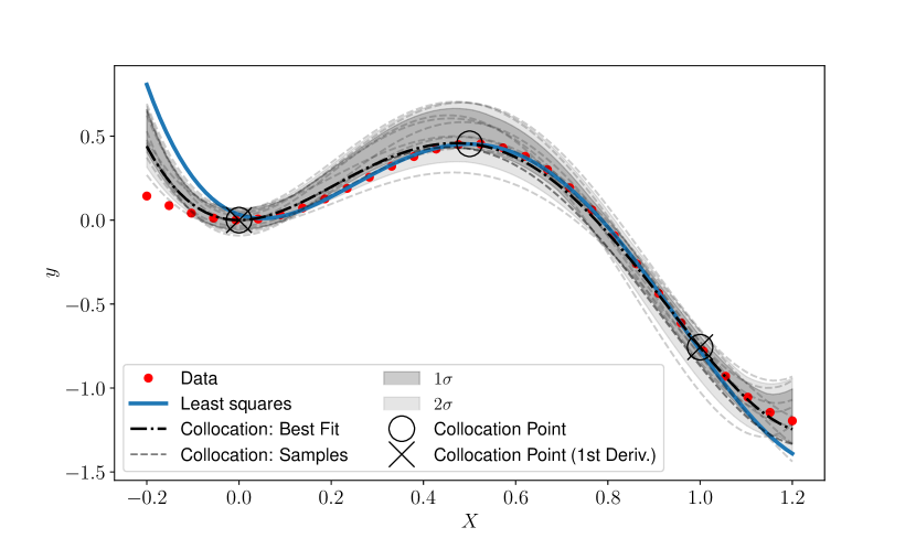
Figure 2: Toy example to illustrate collocation method. We compare the least-squares approach (blue) and the collocation point approach (black/grey) when applied to the task of modelling the data (red). For the collocation point method with specify the value and the first derivative at $x=0$ and $x=1$ as well as a collocation point at $x=0.5$. To generate samples from the collocation point method we perturb the fitted collocation point values with a $\mathcal{N}(0,0.1)$ distribution

V.2 Frequency model

In what follows we use a caret ($\hat{\cdot}$) to indicate a fitted quantity. We split the frequency into three regions which we call the inspiral $\omega_{I}(t)\in[-700,-100]M$, merger $\omega_{M}(t)\in[-100,0]M$, ringdown $\omega_{R}(t)\in[0,87]M$. The times define the regions used for fitting and testing the model.

The inspiral model is written as a correction to the TaylorT3 approximant. We generate the $(\ell,m)=(2,2)$ GW angular frequency, denoted as $\omega_{22}(t)$, using a 3.5 PN order accurate expression for non-spinning binaries  Blanchet et al. (2002); Buonanno et al. (2009) written as

$$\omega_{22}(t) = \omega_{N}(t)\,\sum\limits_{k=0}^{7}\omega_{k}\Theta^{k}\,,$$ (7)

$$\omega_{orb}(t) = \omega_{22}(t)/2\,.$$ (8)

Where $\Theta(t)=\left(\frac{\eta}{5M}(t_{c}-t)\right)^{-1/8}$, $\omega_{k}$ are expansion coefficients Buonanno et al. (2009) and the leading order Newtonian term is given $\omega_{N}(t)=\Theta^{3}(t)/8$. $t_{c}$ is the time which the TaylorT3 expansion formally diverges in what follows we set this value to $t_{c}=0$. Additionally, $\omega_{orb}(t)$ is the orbital angular frequency which is an input for the inspiral amplitude model.

We model the residual between the PN and NR GW angular frequency, factoring out $\omega_{N}$

$$\omega_{res}(t)=\frac{\omega_{NR}(t)-\omega_{22}(t)}{\omega_{N}(t)}\,.$$ (9)

The residual $\omega_{res}(t)$ is evaluated at the following collocation points $T_{\omega}^{I}=\{-700,-300,-100\}M$. Our ansatz to fit this model is given by the next 3 terms in the PN series and therefore extending the PN model to pseudo-5 PN order given by

$$\hat{\omega}_{res}(t)=\sum\limits_{i=0}^{i\leqslant 2}\theta^{\omega_{res}}_{i}\Theta^{8+i}\,.$$ (10)

The model prediction for the inspiral is therefore,

$$\hat{\omega}_{I}(t)=\omega_{22}(t)+\omega_{N}(t)\,\hat{\omega}_{res}(t)\,.$$ (11)

We call the region between the end of the inspiral and the beginning of the ringdown the merger. We found the ansatz proposed in Estellés et al. (2021) to be accurate and adopt it here, as well as for the amplitude model in the next section. The collocation points for this region are $T_{\omega}^{M}=\{-100,-12,0\}M$. The merger ansatz is a power series in arcsinh with a fixed width of $1/\tau$ (where $\tau$ is the damping time of the remnant black hole) given by

$$\hat{\omega}_{M}(t)=\sum\limits_{i=0}^{i\leqslant 2}\theta^{\omega_{M}}_{i}\text{arcsinh}^{i}(t/\tau)\,.$$ (12)

To model the ringdown portion of the waveform we found that a power series in $\tanh$ with a fixed wideth of $1/\tau$ works well. The $\tanh$ function has a logistic shape which matches the phenomenology of the ringdown frequency well. An improvement would be to explicitly include the ringdown frequency prediction from perturbation theory, in a similar way to how the damping time $\tau$ is included. We use the following collocation points $T_{\omega}^{RD}=\{-10,0,10,40\}M$ and the ansatz is given by

$$\hat{\omega}_{RD}(t)=\sum\limits_{i=0}^{i\leqslant 3}\theta^{\omega_{RD}}_{i}\tanh^{i}(t/\tau)\,.$$ (13)

In summary, the following set of frequency coefficients need to be fit as a function of mass-ratio $\theta^{\omega}=\{\theta^{\omega_{res}}\cup\theta^{\omega_{M}}\cup\theta^{\omega_{RD}}\}$ where there is some redundency because the same collocation point is at the boundary between regions. The final inspiral-merger-ringdown angular frequency function is defined piecewise as

$$\hat{\omega}_{IMR}(t)=\begin{cases}\hat{\omega}_{I}(t)&-700M\leqslant t<-100M\\ \hat{\omega}_{M}(t)&-100M\leqslant t<0M\\ \hat{\omega}_{RD}(t)&0M\leqslant t\end{cases}$$ (14)

V.3 Amplitude model

We split the amplitude into four regions which we call the inspiral $A_{I}(t)\in[-700,-300]M$, merger $A_{M}(t)\in[-300,0]M$, early-ringdown (ERD) $A_{ERD}(t)\in[0,30]M$ and late-ringdown (LRD) $A_{LRD}(t)\in[30,87]M$. For the merger and early-ringdown regions we scale the amplitude by $1/\eta$ which approximately removes the variability in the peak amplitude. We decided to split the ringdown into and early- and a late- region to allow us to use linear models and will be discussed below.

The inspiral model is written as a correction to the TaylorT3 approximant. The amplitude of the $(\ell,m)=(2,2)$ mode is expressed as a function of the PN parameter $x$ which is related to the orbital angular frequency by the following relationship

$$x(t)=\omega_{orb}^{2/3}(t)\,.$$ (15)

It is important to use the inspiral frequency model described in the previous section to estimate $\omega_{orb}$ because the PN approximation can become negative at late times causing $x$ to become complex. $x$ is therefore given by $x(t)=(\hat{\omega}_{I}(t)/2)^{2/3}$. The TaylorT3 PN inspiral amplitude is given by

$$A_{PN}(t) = A_{N}(t)\,\hat{H}^{22}(t)\,,$$ (16)

$$A_{N}(t) = 2\eta\sqrt{\frac{16\pi}{5}}x(t)$$ (17)

Where $\hat{H}^{22}(t)$ is an expansion up to 3.5PN Blanchet et al. (2008); Faye et al. (2013) and where we have defined an analogous Newtonian amplitude pre-factor $A_{N}(t)$ which we will use to scale inspiral amplitude residuals by. We first generate the TaylorT3 amplitude and construct the residual between that and the NR data, scaled by $A_{N}$

$$A_{res}(t)=\frac{A_{NR}(t)-A_{PN}(t)}{A_{N}(t)}\,.$$ (18)

Similarly to the inspiral frequency model we define our amplitude inspiral ansatz as an extension of the PN model up to 4.5 PN order given by

$$\hat{A}_{res}(t)=\sum\limits_{i=0}^{i\leqslant 1}\theta^{A_{res}}_{i}x^{(8+i)/2}(t)\,.$$ (19)

We only use two collocation points $T_{A}^{I}=\{-700,-100\}M$ as we find that the majority of the amplitude data is explained well by our inspiral frequency model $\hat{\omega_{I}}$. The inspiral amplitude model is given by

$$\hat{A}_{I}(t)=A_{PN}(t)+A_{N}(t)\,\hat{A}_{res}(t)\,.$$ (20)

For the amplitude merger region, contrary to Estellés et al. (2021) who chose an ansatz based on the sech function, we use a power series in arcsinh with a width of $1/\tau$

$$\hat{A}_{M}(t)=\sum\limits_{i=0}^{i\leqslant 3}\theta^{A_{M}}_{i}\text{arcsinh}^{i}(t/\tau)\,,$$ (21)

with collocation points given by $T_{A}^{M}=\{-100,-50,-10,0\}M$.

The behaviour of the waveform after the peak of the amplitude is typically called the ringdown region however, it is an active area of research to determine the correct physics to describe the transtion the merger to the ringdown Giesler et al. (2019); Cook (2020); Jiménez Forteza et al. (2020); Forteza and Mourier (2021). In recent years time domain waveform models tend to use the non-linear model presented in Damour and Nagar (2014) to model the ringdown region from the peak amplitude onwards. However, because the standard collocation point method we use requires linear ansätze we are unable to use this ringdown parameterisation. Instead, we have introduced an “early-ringdown” region to bridge the gap between the peak amplitude and the start of the ringdown region which we loosely to be the times that can be accurately approximated by black hole perturbation theory. Motivated by the similarity between the onset and falloff of the waveform around the peak we model the early-ringdown with the same ansatz that we use for the merger amplitude. The early-ringdown ansatz is

$$\hat{A}_{ERD}(t)=\sum\limits_{i=0}^{i\leqslant 4}\theta^{A_{ERD}}_{i}\text{arcsinh}^{i}(t/\tau)\,.$$ (22)

The collocation points are $t_{ERD}=\{0,5,20,30\}M$ with an additional collocation point evaluating the derivative of the peak amplitude $t_{ERD}^{\prime}=\{0\}M$. The full set of collocation points is therefore, $T_{A}^{ERD}=t_{ERD}\cup t_{ERD}^{\prime}$. As we expect the derivative at the peak to be zero we enforce this manually instead of fitting the collocation values for the collocation point $t_{ERD}^{\prime}$.

The late-ringdown ansatz is simply exponential decay with a decay constant equal to the damping frequency of the remnant black hole $1/\tau$.

$$\hat{A}_{LRD}(t)=\beta_{LRD}e^{-t/\tau}\,.$$ (23)

The constant $\beta_{LRD}$ is fixed by enforcing C(0) continuity and is defined as

$$\beta_{LRD}=\hat{A}_{ERD}(t_{0})e^{t_{0}/\tau}\,.$$ (24)

The matching time is a constant value of $t_{0}=30M$. Defining a time after the peak amplitude where the system can be fully described by perturbation theory is an active area of research. For our purposes we need an approximate time after which we can accurate transition to a purely exponential decay model.

In summary the following set of amplitude coefficients need to be fit as a function of mass-ratio $\theta^{A}=\{\theta^{A_{res}}\cup\theta^{A_{M}}\cup\theta^{A_{ERD}}\}$. The final inspiral-merger-ringdown amplitude function is defined piecewise as

$$\hat{A}_{IMR}(t)=\begin{cases}\hat{A}_{I}(t)&-700M\leqslant t<-100M\\ \hat{A}_{M}(t)&-100M\leqslant t<0M\\ \hat{A}_{ERD}(t)&0M\leqslant t<30M\\ \hat{A}_{LRD}(t)&30M\leqslant t\end{cases}$$ (25)

VI Non-parametric model

In this section we describe our non-parametric model for the parameter space fits needed to go from a discrete set of data samples to a continuous model over the parameter space.

The target data is the set of all collocation values for both the amplitude and frequency models described in the previous section. We gather the collocation values together as $\theta=\{\theta^{A}\cup\theta^{\omega}\}$. For each collocation value we will construct a non-parametric model as a function of the mass-ratio i.e. $g_{\theta}(q)$. To do this we will use the Gaussian process regression algorithm. The GPR algorithm begins by placing a Gaussian process prior over the quantity of interest written as

$$g_{\theta}(q)\sim\mathcal{GP}(m_{\theta}(q),k_{\theta}(q,q^{\prime}))\,,$$ (26)

with mean $m_{\theta}(q)$ and covariance function $k_{\theta}(q,q^{\prime})$ for the $\theta$ collocation point. Here, the GP model is simply multi-dimensional Normal distribution with a covariance matrix constructed from the training set according to a prescribed covariance function $k(q,q^{\prime})$. We choose $m_{\theta}(q)=0$ and for the covariance function we use the Matérn kernel (with smoothness parameter $\nu=5/2$) Rasmussen and Williams (2006).

The kernel hyperparameters were determined by numerically optimising the log marginal likelihood of the GP. We use the scikit-learn Pedregosa et al. (2011) implementation of Gaussian Process Regresssion in our prototype model. A production-ready model would require either; a more computationally performant GPR implementation, fast approximations such as sparse-variational, random fourier features Rahimi and Recht (2007); Wilson et al. (2020) or harware accelerators such as GPUs.

We found it necessary to transform the target variable to enforce the model to make predictions that could not change sign, this could happen when the target values are close to zero. For the amplitude and frequency data this is a physical constraint. To constrain the model to only predict positve values we exponentiate it’s predictions and therefore we define the transformed target variable as $z$ through the following equation

$$z:=\log(\,|\,y\,|\,)\,.$$ (27)

Where $y$ is the target variable (i.e. collocation point values). We can reverse this transformation so long as we keep track of the original sign of $y$. Additionally, we also found that modelling $\log(q)$ helped to improve the extrapolation behaviour of the GP.

Next we discuss two types of uncertainty that our method accounts for. For the purposes of our fit of the collocation points we consider the variance between collocation values at the same mass-ratio as the statistical (also called aleatoric or data) uncertainty and the variance in regions devoid of training data is called the systematic (also called epistemic or model) uncertainty of the waveform model.

The statistical uncertainty is quantified by measuring the accuracy of NR solutions (for example via a numerical convergence series) and can be reduced by producing more accurate NR solutions. The systematic uncertainty is a measure of how well the model fit is constrained by the training data. To reduce the systematic uncertainty you can perform new NR simulations at regions where the model predicts large systematic uncertainty. From the perspective of NR it is known that simulations of high mass-ratio and/or rapidly rotating BHs are typically much harder, numerically speaking, to simulate and therefore, it is conceivable to expect the NR error to be larger in these regions of parameter space. In lieu of a full convergence series for each NR simulation in our training set we take a conservative approach and assume each simulation is equally accurate. We use a homoskedastic noise model assuming a constant noise variance which is an additional hyperparameter informed by the measured variance in the training data.

The systematic uncertainty in GPR models can be controlled by the kernel function. Our choice of using a stationary kernel such as the Matérn endows the model with a notion of distance from the training set and as such can produce models with the desired property that have larger uncertainty for points outside the training set.

Figure 3 shows the GPR fit for the peak amplitude (collocation point at $t=0M$). The blue and orange points are the training and test sets respectively. The red line is the GPR mean, the red shaded region is the $2\sigma$ predictive interval. As we extrapolate the GP model towards mass-ratio 32:1 (the largest mass-ratio simulation in the test set) we find that the mean prediction agrees well however, the uncertainty also grows.

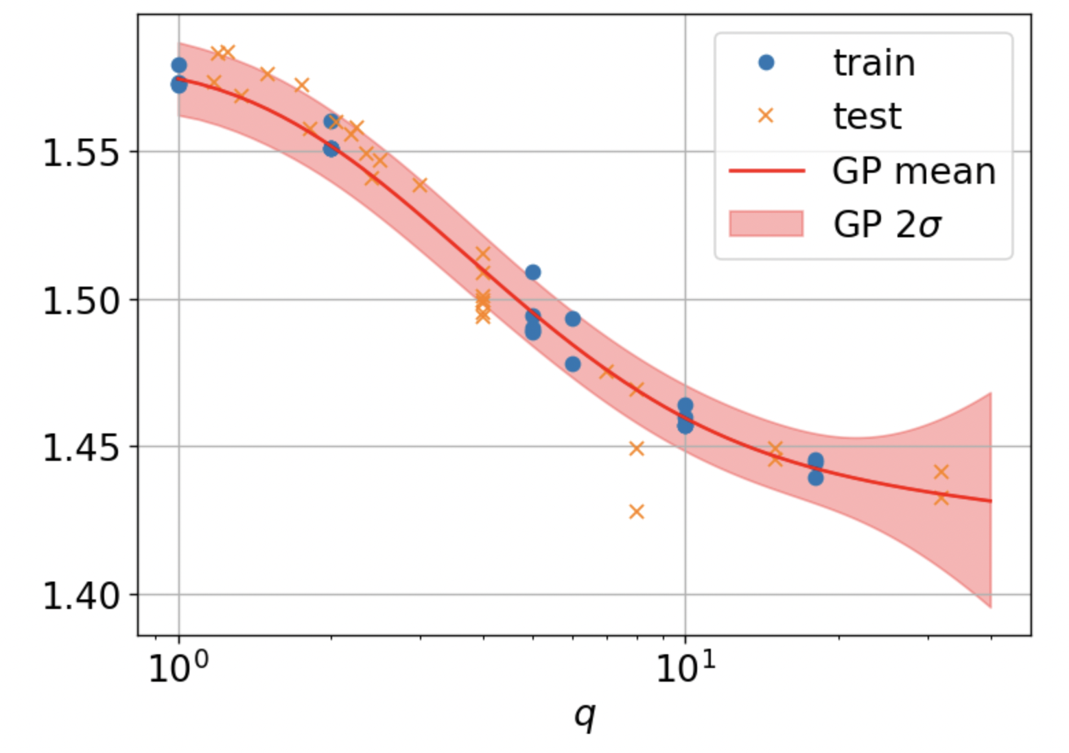
Figure 3: Example GPR fit for the amplitude merger model. We show the data and fit for the collocation point at time $t=0M$. The training and test set are shown as blue and orange points. The mean GP fit is the red line and the red shaded region is the $2\sigma$ prediction interval.

VII Final Model

As a reminder, we model the amplitude and angular frequency of the $h_{22}$ complex multipole using a set of linear ansätze. The free parameters (collocation point values) are modelled independently as a probability distribution that depends on the mass-ratio using GPR. We denote the GP fit to collocation point value $\theta$ belonging to either the amplitude (A) or angular frequency ($\omega$) as $g_{\theta^{[A/\omega]}}(q)$. Using this, we define the final model for the complex multipole as

$$p(\hat{h}_{22}|t,q) \equiv p(\hat{h}_{22}|t,g_{\theta}(q))$$ (28)

$$= \hat{A}_{IMR}(t,g_{\theta^{A}}(q))\exp\left[{-i\hat{\phi}_{IMR}(t,g_{\theta^{\omega}}(q))}\right]\,.$$ (29)

The model for the GW phase $\hat{\phi}_{IMR}$ is obtained by generating $\hat{\omega}_{IMR}$ first and then numerically integrating it however, an analyitc expression could be derived. $\hat{A}_{IMR}$ and $\hat{\omega}_{IMR}$ are given by Eq. 25 and Eq. 14 respectively.

The GPR method provides an analytic expression for the mean of the GP which we will denote as $\bar{\theta}(q)$. The mean prediction (which could also be called the best-fit prediction) is obtained when we use the mean of each GP fit as the estimate for the collocation values. We define this as

$$\bar{h}_{22}(t,q)\equiv p(\hat{h}_{22}|t,g_{\bar{\theta}}(q))\,.$$ (30)

The model can produce independent waveform realisations, denoted by $\tilde{h}$, by drawing a random sample from the posterior probability for each $\theta$. We define this as

$$\tilde{h}\sim p(\hat{h}_{22}|t,g_{\theta}(q))\,.$$ (31)

The ability to draw waveform samples can be utilised in Bayesian parameter estimation of GW events in order to marginalise the posterior over waveform systematic and statistical uncertainty.

VIII Model validation

To assess the accuracy between two real-valued time-domain waveforms $h_{1}$ and $h_{2}$ we use the noise-weighted inner product

$$\langle h_{1},h_{2}\rangle=4\,\text{Re}\int\limits_{f_{\text{min}}}^{f_{\text{max}}}\frac{\tilde{h}_{1}(f)\tilde{h}_{2}^{*}(f)}{S_{n}(f)}df\,.$$ (32)

Where $S_{n}(f)$ is the noise power spectral density of the detector. The match is defined as the inner product between normalised waveforms $(\hat{h}=h/\sqrt{\langle h,h\rangle})$ maximised over a relative time and phase shift between $h_{1}$ and $h_{2}$. Our main accuracy metric is the mismatch $\mathcal{M}$ defined as,

$$\mathcal{M}(h_{1},h_{2})=1-\max\limits_{t_{0},\phi_{0}}\langle\hat{h}_{1},\hat{h}_{2}\rangle\,.$$ (33)

Because the NR data are relatively short (when the total mass is scaled to $100M_{\odot}$ the start frequency ranges from $20-30$ Hz) we choose to compute the white-noise mismatch. We do not wish to introduce uncertainty into our results due to the inability of the NR data to fill the detectors sensitivity band at a given total mass Ohme et al. (2011) or introduce an ambiguity into which part of the waveform is responsible for the error. In what follows we generate waveforms with a sample rate of $4096$ Hz scaled to a total mass of $100M_{\odot}$.

Figure 4 shows the results of the mismatch calculation. We compute the mismatch between the mean PPM waveform and every NR solution in the train (circle) and test (filled circle) set. The points are coloured with respect to the NR code used to generate them.

The median mismatch across the test set is $0.13\%$ (a match of $99.87\%$). The worst mismatch over the test set is $11\%$ (a match of $89\%$) which occurs for the 32:1 simulation. As this simulation is far away from any training data and we haven’t specifically tuned how the model should extrapolate it is not surprising that the error is large. The next worst mismatch is $0.32\%$ (a match of $99.68\%$) which occurs for mass-ratio 3:1. A baseline accuracy threshold of $1\%$ mismatch error is typically used for which the PPM model passes for mass-ratios less than 18:1.

To illustrate the uncertainty in the NR waveforms we compute the mismatch between a reference NR waveform and all other NR waveforms at the same mass-ratio, these are shown as black circles. This estimate for the NR error tends to give error estimates with larger variances when there are more than one NR code available to compare. For example, simulations at mass-ratios 8:1 and 18:1 are only available with the BAM NR code. This estimate should be treated with caution as it assumes all the NR waveforms used in the comparison are of comparable numerical accuracy which is not true. For instance, we have included NR waveforms from the same code but performed at different numerical resolutions. Future NR simulations available at multiple resolutions that permit a convergence test would alleviate this issue.

Our PPM can be used to empirically estimate its own uncertainty. We call this the predicted mismatch distribution $p_{\mathcal{M}}$ and it is computed as the distribution of the mismatch between the mean PPM waveform ($\bar{h}^{PPM}$) and 1000 samples ($\tilde{h}^{PPM}$) from the PPM model.

$$p_{\mathcal{M}}=\mathcal{M}(\bar{h}^{PPM},\tilde{h}^{PPM})\,.$$ (34)

In Figure 4 we show the median of $p_{\mathcal{M}}$ as a solid blue line as well as the $50^{th}$, $90^{th}$ and $99^{th}$ percentile widths as shaded blue regions. The results show that the model predicts its error to be relatively constant between mass-ratio 1:1 and 10:1 at the level of $0.019_{-0.015}^{+0.039}\%$. The behaviour between 10:1 and 18:1 suggests that the uncertainty estimate for the 18:1 is too small resulting in a GP model that is too heavily constrained in the vicinity of the 18:1 data and can cause the observed high variance predictions. Using our prediction for the expected mismatch we state that we expect the PPM model to likely (at the $99^{th}\%$) still be accurate at approximately the $1\%$ level when extrapolated to mass-ratio 20:1. In the next section we will quantify the accuracy of this estimate.

There are a number of simulations in the test set, at low mass-ratio between 1:1 and 4:1, that have unusually high mismatches when compared with the PPM mean model as well as lie outside the predicted mismatch distribution. Simulations at nearby mass-ratios are available from different NR codes and the difference seen suggests that the Maya simulations in this region and the BAM 4:1 simulations have numerical errors larger than the other NR codes in our dataset. This highlights the potential benefits from constructing training sets from multiple NR codes to avoid building models that inherit potential systematic biases from particular NR simulations.

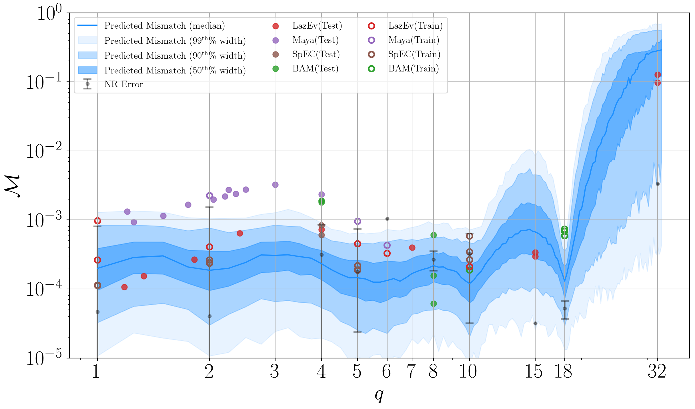
Figure 4: The mismatch between various objects as a function of the mass-ratio. The black error bars are an estimate of the NR uncertainty obtained by computing the mismatch between NR waveforms at the same mass-ratio. The mismatch between PPM mean prediction and NR simulations in the training set (open circles) and the test set (filled circles), which are coloured based on the NR code, represent the typical accuracy metric of waveform models. The solid blue curve is the median of the predicted mismatch distribution (Eq. 34) and the shaded blue regions show the $50^{th}$, $90^{th}$ and $99^{th}$ percentile widths.

Next we compare the PPM model predictions with NR waveforms in the test set to illustrate how the diversity in waveform predictions under different levels of uncertainty. Figure 5 shows the $h_{+}$ waveform from NR (black, dashed) and predictions from PPM (blue). Both the mean and 3 samples from PPM are shown as well as the minimum and maximum values from 1000 samples are shown as the shaded region. From top to bottom we show mass-ratios 4:1, 8:1, 15:1 and 32:1, the mismatch between the mean PPM prediction and NR is $0.18\%$, $0.016\%$, $0.032\%$ and $11\%$ respectively. The self-mismatch error for 4:1 and 8:1 are both $0.05\%$ (worst mismatch at $90^{th}$ percentile), this level of variance in mismatch corresponds to practically indistinguishable predictions between PPM samples on this scale. As the mass-ratio increases visible differences begin to be noticeable at mass-ratio 15:1 where the self-mismatch error gets to the $0.5\%$ (worst mismatch at $90^{th}$ percentile) level. For mass-ratio 32:1 the samples from the PPM model are very diverse which gives rise to a large mean predicted mismatch ($28\%$) and a wide distribution with mismatches reaching up to $57\%$ (worst mismatch at $90^{th}$ percentile) for the predicted mismatch distribution.

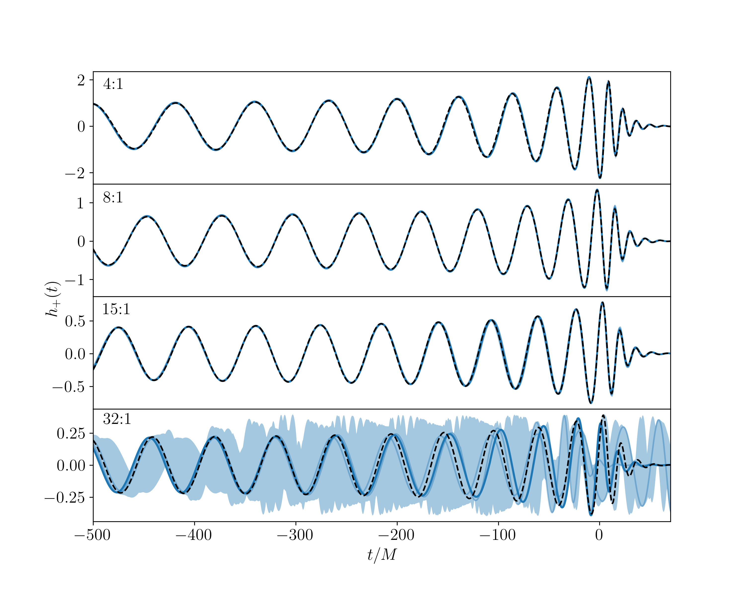
Figure 5: In each panel we compare our model with representatative NR simulations at mass-ratios 4:1. 8:1, 15:1 and 32:1 from the test set. The NR is shown as a solid black line. We generate 1000 samples and the mean prediction from our PPM model and optimally align them with the NR waveform over a time and phase shift. We show the minimum and maximum range of values from the 1000 samples as the shaded region and explicitly plot the mean as well as 3 samples.

IX Uncertainty Calibration

In the previous section we have shown how probabilistic models can be used to estimate their uncertainty with the use of the predicted mismatch distribution. However, having the ability to generate waveform samples does not guarantee that the resulting distribution of waveforms will accurately represent the true uncertainty of the model. In this section we quantify the accuracy of our uncertainty prediction.

We compare the estimated uncertainty with the true uncertainty of the model at the train and test locations to quantity the accuracy of the uncertainty estimate. For the true uncertainty we use the mismatch between NR waveforms and the PPM mean waveform. We summarise the results with a metric we call the calibration score $\mathcal{C}$ defined as the ratio between the true uncertainty and the estimated uncertainty (both measured in terms of the mismatch)

$$\mathcal{C}=\frac{\text{True Uncertainty}}{\text{Estimated Uncertainty}}$$ (35)

For the estimated uncertainty we use the predicted mismatch distribution $p_{\mathcal{M}}(q)$ (Eq. 34) from the previous section to obtain a distribution for the calibration score

$$p_{\mathcal{C}}(q)=\frac{\mathcal{M}(\bar{h}^{PPM},h^{NR})}{p_{\mathcal{M}}(q)}\,.$$ (36)

A perfectly calibrated model will have $\mathcal{C}=1$. A model that is underestimating the uncertainty and is therefore overconfident will have $\mathcal{C}>1$, here samples from the PPM will be closer to the mean prediction than they should be. A model that is overestimating the uncertainty and is therefore underconfident will have $\mathcal{C}<1$, here samples from the PPM will be further from the mean prediction than they should be.

A previous study Doctor et al. (2017) that also used GPR in waveform modelling proposed to use the maximum mismatch between the mean waveform and waveform samples to estimate the true uncertainty i.e. $\max p_{\mathcal{M}}$. This typically results in estimates of the calibration score that are biased towards being underconfident.

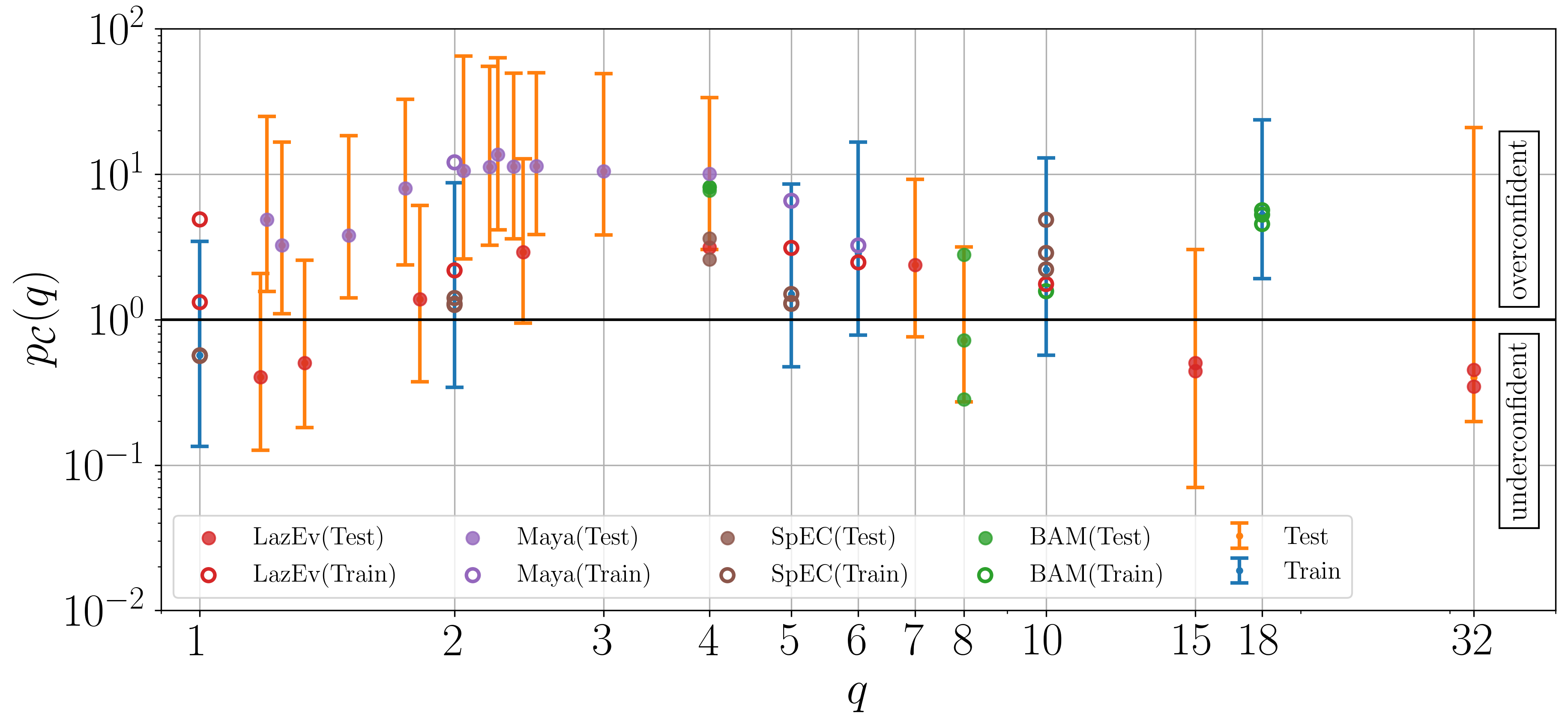
Figure 6: Calibration score distribution as defined by Equation 36. We show the median value and the $90\%$ width of the predicted mismatch distribution for the train (blue) and test (orange) sets. We also show the individual results for each NR simulation compared with the median value of the predicted mismatch.

The calibration score as a function of the mass-ratio is shown in Figure 6. For each mass-ratio where we have more than one NR simulation we aggregate the results and show the median as well as the $90\%$ width of the predicted mismatch distribution. These results are shown as blue and orange points for the train and test sets respectively. We also show $\mathcal{C}$ for each individual NR simulation computed using the median value of the predicted mismatch distribution. These results are shown as circles and filled-circles for the train and test sets respectively.

For the train set we find that the calibration score is consistent with 1 at the $90\%$ level for all mass-ratios except the 18:1 simulations. Here the model is overconfident in its predictions by a factor of 5 on average. For the test set we find our model produces calibrated uncertainties for all cases at the $90\%$ level except the mass-ratio 4:1 and all Maya simulations between mass-ratio 1:1 and 4:1. For these cases the model is consistently overconfident in its uncertainty estimate.

Our calculation for the calibration score is potentially corrupted due to data quality issues with the NR data. In this work we have attempted to control for this by including as many NR simulations from different codes as possible however, there simply isn’t enough data. For example, waveforms in the test set for $q>1$ and $q<4$ are mainly from the Maya NR code which could potentially be a cause of systematic bias in our estimates. Also we are treating NR solutions with different numerical resolutions as being equally accurate.

We hypothesise that the main source of error that is reducing the ability of our model to accurately predict the true uncertainty is due to data quality issues which violates our assumption that the NR data are of sufficient and comparable accuracy. The evidence for this is can be seen in Figure 4 where the Maya $q\in(1,4]$ and the BAM $q=4$ simulations have higher mismatch errors then the other NR simulations when compared with the PPM model. Typically these simulations would not be included in the data set due to data quality concerns however, without a full convergence series for an NR simulation it is difficult to quantify the errors in a simulation. However, if the errors in a simulation are quantified appropriately then these simulations may still add valuable information but their influence will be downweighted.

X Conclusions

In this paper we address the increasingly important issue of uncertainty quantification in waveform modelling. We have presented a new methodology to build probabilistic phenomenological models (PPMs). The key aspects of our work are: (i) employing linear ansätze so we can use the collocation fitting method and gain interpretability, (ii) using a probabilistic fitting method (such as Gaussian process regression) for the parameter space fits and (iii) using estimates for the NR uncertainty to inform those fits. PPMs extend current phenomenological methods with the ability to not only generate the best-fit point estimate but also explicit waveform samples that can be used to marginalise over waveform model errors in GW Bayesian parameter estimation.

The model presented here is a proof of concept. It only covers a small portion of the waveform ($\sim 800M$ in duration) and does not model spinning binaries. It should be relatively straightforward to adapt current methodology used to build deterministic phenomenological models, that model precessing binaries with higher order multipoles, and turn them into probabilistic phenomenological models. NR solutions of these more complete descriptions of binary coalescence typically have larger numerical errors and therefore stand to benefit the most from a probabilistic treatment.

Some interesting technical challenges have the potential to appear when increasing the size of the dataset and/or including more physics. For example, the noise model assumption may need to be revised if the data shows sign of heteroskedasticity. Another assumption is the independence of the phenomenological coefficients. Future models will likely continue using non-linear ansätze that are more physically motivated. If the coefficients of these models have significant correlation then our method of sampling the coefficients independently could result in unphysical waveforms. In such a case then modelling algorithms that can jointly model the coefficients will have to be explored.

The most important issue that needs to be resolved is to improve the error estimates in NR simulations as this is a crucial ingredient in modelling. We have experiemented with using the difference between NR solutions from different NR codes to estimate the NR error however, this is not reliable. Where possible we recommend NR groups publish detailed uncertainty estimates that are functions of time along with their waveforms.