Towards Scalable Semidefinite Programming: Optimal Metric ADMM with A Worst-case Performance Guarantee

Abstract

Despite the numerous uses of semidefinite programming (SDP) and its universal solvability via interior point methods (IPMs), it is rarely applied to practical large-scale problems. This mainly owes to the computational cost of IPMs that increases in a bad exponential way with the data size. While first-order algorithms such as ADMM can alleviate this issue, but the scalability improvement appears far not enough. In this work, we aim to achieve extra acceleration for ADMM by appealing to a non-Euclidean metric space, while maintaining everything in closed-form expressions. The efficiency gain comes from the extra degrees of freedom of a variable metric compared to a scalar step-size, which allows us to capture some additional ill-conditioning structures.

On the application side, we consider the quadratically constrained quadratic program (QCQP), which naturally appears in an SDP form after a dualization procedure. This technique, known as semidefinite relaxation, has important uses across different fields, particularly in wireless communications. Numerically, we observe that the scalability property is significantly improved. Depending on the data generation process, the extra acceleration can easily surpass the scalar-parameter efficiency limit, and the advantage is rapidly increasing as the data conditioning becomes worse.

Keywords:  Semidefinite programming, Variable metric methods, Preconditioning, Parameter selection, Duality, Quadratically constrained quadratic program, Alternating Direction Method of Multipliers (ADMM)

1 Introduction

Semidefinite programming (SDP) [1, 2, 3, 4, 5] is widely recognized as one of the most important breakthroughs in the last century. It is developed as a generalization to linear programming (LP), and is not much harder to solve [1]. The solvability issue is perfectly addressed by the interior-point methods (IPMs), which were first introduced in 1984 by Karmarkar [6] for LP, and later extended to all convex programs by Nesterov and Nemirovsky in 1988 [7, 8, 9, 10]. Many well-known convex solvers such as CVX [11], and MOSEK [12] are built on the IPMs. Despite the great successes, the IPMs are not well-suited to a newly arisen challenge, ‘Big Data’. This is due to its second-order nature that involves Hessian information. The Hessian is in general a dense matrix even when the data is highly structured. The computational cost is therefore in general prohibitively expensive for large-scale data. In the literature, first-order algorithms (FOAs) that only use gradient (or subgradient) information are considered one of the most promising tools for large-scale problems, see a comprehensive survey paper by Amir Beck [13], and a simplified view by Marc Teboulle [14].

Among the large class of FOAs, ADMM has received an increasing amount of attention. This partly owes to its outstanding practical performance and also elegant theory, see a survey paper by Stephen Boyd et. al. [15]. The ADMM algorithm itself is not new, originally proposed by Glowinski and Marrocco [16] in 1975, and Gabay and Mercier [17] in 1976. It is known to be equivalent to some popular algorithms from other fields. The perhaps most important one is the Douglas-Rachford Splitting (DRS) [18, 19, 20, 21] in numerical analysis. Due to their equivalence, the ADMM is typically analysed by converting to the DRS, and invoking the fixed-point theory [22, 23]. Most recently, Yifan Ran established a direct fixed-point analysis for ADMM (that does not need DRS), see [24, sec. 6]. Additionally, the Primal-Dual Hybrid Gradient (PDHG) method [25, 26, 27] is also shown to be equivalent to ADMM, see O’Connor and Vandenberghe [28]. Apart from being equivalent, some strong connections are known between ADMM and Spingarn’s method of partial inverses, Dykstra’s alternating projections method, Bregman iterative algorithms for $l_{1}$ problems in signal processing, see more details from [15].

In the literature, different FOAs for solving SDP mainly differ in how the positive semidefinite (PSD) constraint is handled. One typical approach is by noting that any PSD matrix can be characterized by $\bm{R}^{T}\bm{R}$. Hence, the PSD requirement is removed if the variable is substituted to $\bm{R}$, see related works in [29, 30, 31]. It is worth noticing that the efficiency of this approach highly depends on the dimension of $\bm{R}$. Indeed, if the underlying solution is low-rank, $\bm{R}$ admits very few columns and the problem could be solved efficiently. Another way is to enforce the PSD requirement by a new projected variable, i.e., $\Pi_{\mathbb{S}^{N}_{+}}(\bm{X})$, where $\Pi_{\mathbb{S}^{N}_{+}}$ is a projector onto the PSD cone, equivalent to setting all negative eigenvalues to zeros. Owing to such a projector being strongly semi-smooth [32], an inexact semi-smooth Newton-CG method is designed, see [33]. The last approach is via ADMM, which handles the PSD requirement by introducing an auxiliary variable and performs a projection $\Pi_{\mathbb{S}^{N}_{+}}$ separately, see a typical success in [34].

Despite the successes of FOAs, they share a common weakness — their performances highly depend on the conditioning of the data. The technique for addressing this issue is known as preconditioning. A typical heuristic to select a preconditioner is by appealing to the condition number, where, given a linear system $\bm{Ax}=\bm{b}$, one rewrites it into $\bm{EAx}=\bm{Eb}$, and selects the preconditioner $\bm{E}$ such that the new matrix $\bm{EA}$ has a smaller condition number (the largest eigenvalue divide the smallest eigenvalue). This approach is well-known and perhaps the most popular one. However, we emphasize that it is in nature a heuristic. That said, even when the condition number is minimized, there is no guarantee that the algorithm convergence rate will be improved. Indeed, how to select the preconditioner to optimize the convergence rate is open, see e.g. [35, sec. 1.2, First-order methods], [23, sec.8, Parameter selection]. Due to the lack of optimal choice, the preconditioner is typically manually tuned in practice. However, manual tuning is problematic. First, for a matrix preconditioner, there exist multiple parameters, depending on the degrees of freedom. How to simultaneously tune them seems to be a huge obstacle. Even when tuning a scalar, the fine-tuned choice is likely not transferable to other types of data, or simply different data sizes. Indeed, we note that in [33], the authors fix the step-size parameter to either $1$ or $1.6$, without adapting it to different input data.

Most recently, such an optimal parameter issue has been addressed by Yifan Ran, where the author optimizes a general worst-case convergence rate without strong assumptions, see the scalar case in [36] and the metric space case in [24]. In either case, the optimal parameter choice can be determined by solving a degree-4 polynomial. Except, in the scalar setting, a closed-form optimal solution always exists regardless of the initialization choice; in a non-Euclidean metric space, despite the potential extra acceleration, a closed-form expression for both the metric choice and the algorithm iterates are not guaranteed.

In this work, we consider the metric space case in order to gain extra acceleration. We will address the closed-form issue. To our best knowledge, there is no metric-type ADMM applied to SDP in the literature. This is likely due to the aforementioned projection step $\Pi_{\mathbb{S}^{N}_{+}}$ no longer works in a non-Euclidean space, i.e., it is not a feasible ADMM iterate. Indeed, we will show that, given a special class of (decomposed) metrics $\mathcal{S}$, the feasible projection step would be $\mathcal{S}^{-1}\Pi_{\mathbb{S}^{N}_{+}}\mathcal{S}$.

On the application side, we consider the quadratically constrained quadratic program (QCQP). It is NP-hard and non-convex in nature. A typical approach, known as semidefinite relaxation, can reformulate it into an SDP. This technique plays a fundamental role in wireless communications, see a survey paper [37] and references therein. We will present the first metric-type ADMM solver for the convexified QCQP and numerically evaluate its performance.

1.1 Notations

The Euclidean space is denoted by $\mathscr{H}$ with inner product $\langle\cdot,\,\cdot\rangle$ equipped, and its induced norm $\|\cdot\|$. We denote its extension to a metric space as $\mathscr{H}_{\mathcal{M}}$, with norm $\|\bm{v}\|_{\mathcal{M}}=\sqrt{\langle\bm{v},\mathcal{M}\bm{v}\rangle}$. We denote by $\Gamma_{0}(\mathscr{H})$ the space of convex, closed and proper (CCP) functions from $\mathscr{H}$ to the extended real line $]-\infty,+\infty]$, by $\mathbb{S}^{N}$, the space of $N$-dimensional symmetric matrices, by $\mathbb{S}^{N}_{+}$, the space of $N$-dimensional positive semidefinite matrices. At last, the uppercase bold, lowercase bold, and not bold letters are used for matrices, vectors, and scalars, respectively. The uppercase calligraphic letters, such as $\mathcal{A}$ are used to denote operators.

1.2 ADMM algorithm

The ADMM algorithm solves the following general convex problem:

$$\,\underset{\bm{x},\bm{z}}{\text{minimize}}\quad f(\bm{x})+g(\bm{z})$$

$$\text{subject\,to}\quad\mathcal{A}\bm{x}-\mathcal{B}\bm{z}=\bm{c},$$ (1.1)

with functions $f,g\in\Gamma_{0}(\mathscr{H})$ and operators $\mathcal{A},\,\mathcal{B}$ being injective. Moreover, we assume a solution exists.

1.2.1 Basic iterates

The basic ADMM iterates are based on the following augmented Lagrangian:

$$\mathcal{L}_{\gamma}(\bm{x},\bm{z},\bm{\lambda})\,=\,f(\bm{x})+g(\bm{z})+\frac{\gamma}{2}\|\mathcal{A}\bm{x}-\mathcal{B}\bm{z}-\bm{c}+\bm{\lambda}/\gamma\|^{2},$$ (1.2)

where $\gamma>0$ denotes a positive step-size. The ADMM iterates are

$$\bm{x}^{k+1}=\,\, \underset{\bm{x}}{\text{argmin}}\,\,\mathcal{L}_{\gamma}(\bm{x},\bm{z}^{k},\bm{\lambda}^{k})$$

$$\bm{z}^{k+1}=\,\, \underset{\bm{z}}{\text{argmin}}\,\,\mathcal{L}_{\gamma}(\bm{x}^{k+1},\bm{z},\bm{\lambda}^{k})$$

$$\bm{\lambda}^{k+1}=\,\, \bm{\lambda}^{k}+\gamma(\mathcal{A}\bm{x}^{k+1}-\mathcal{B}\bm{z}^{k+1}-\bm{c}),$$ (scalar ADMM)

which are guaranteed to converge (if minimizers exist) with any positive step-size $\gamma>0$.

1.2.2 Metric space iterates

The above $\gamma$-parametrized iterates can be extended to a metric space environment $\mathscr{H}_{\mathcal{M}}$, with the following augmented Lagrangian:

$$\mathcal{L}_{\mathcal{M}}(\bm{x},\bm{z},\bm{\lambda})\,=\,f(\bm{x})+g(\bm{z})+\frac{1}{2}\|\mathcal{A}\bm{x}-\mathcal{B}\bm{z}+\mathcal{M}^{-1}\bm{\lambda}\|^{2}_{\mathcal{M}},$$ (1.3)

with norm $\|\bm{v}\|_{\mathcal{M}}=\sqrt{\langle\bm{v},\mathcal{M}\bm{v}\rangle}$. The ADMM iterates are

$$\bm{x}^{k+1}=\,\, \underset{\bm{x}}{\text{argmin}}\,\,\mathcal{L}_{\mathcal{M}}(\bm{x},\bm{z}^{k},\bm{\lambda}^{k})$$

$$\bm{z}^{k+1}=\,\, \underset{\bm{z}}{\text{argmin}}\,\,\mathcal{L}_{\mathcal{M}}(\bm{x}^{k+1},\bm{z},\bm{\lambda}^{k})$$

$$\bm{\lambda}^{k+1}=\,\, \bm{\lambda}^{k}+\mathcal{M}(\mathcal{A}\bm{x}^{k+1}-\mathcal{B}\bm{z}^{k+1}-\bm{c}),$$ (metric ADMM)

which are guaranteed to converge (if minimizers exist) with any positive definite metric $\mathcal{M}\succ 0$.

1.3 Semidefinite programming

Semidefinite programming (SDP) considers minimizing a linear function of variable $\bm{x}\in\mathbb{R}^{m}$ subject to a Linear Matrix Inequality (LMI). The standard form is given below, see e.g. [1]:

$$\underset{\bm{x}}{\text{minimize}}\quad \langle\bm{c},\bm{x}\rangle$$

subject to $$\bm{A}_{0}+\sum_{i=1}^{m}x_{i}\bm{A}_{i}\succeq 0.$$ (Primal)

with $\bm{A}_{i}\in\mathbb{S}^{N},\,\,i=0,1,\dots,m$ being symmetric matrices. Its Fenchel dual problem is

$$\qquad\qquad\,\,\underset{\bm{X}}{\text{minimize}}\quad\,\,\, \langle\bm{A}_{0},\bm{X}\rangle$$

subject to $$\langle\bm{A}_{i},\bm{X}\rangle=c_{i},\quad i=1,\dots,m$$

$$\,\,\bm{X}\succeq 0.$$ (Dual)

2 Preliminary: a unified treatment

To start, we show that (1.3) and (1.3) share the same intrinsic structure, and can be handled in a unified way, via

$$\,\underset{\bm{X},\bm{Z}}{\text{minimize}}\quad\,f\,(\bm{X})+\delta_{\mathbb{S}^{N}_{+}}(\bm{Z})\qquad$$

$$\text{subject\,to}\quad\mathcal{A}\,\big{(}\bm{X}\big{)}=\bm{Z}.\qquad$$ (Unified)

For (LABEL:pri), the matrix variable $\bm{X}$ reduces to a vector $\bm{x}$, and the following definitions are used:

$$\quad(\text{Function})\qquad\,\,\, \,f\,(\bm{x})\,\overset{\mathclap{\text{def}}}{=}\,\,\langle\bm{c},\bm{x}\rangle,\qquad\text{dom}\,f=\mathscr{H}$$

$$\,\,(\text{Constraint})\qquad \mathcal{A}\,\big{(}\bm{x}\big{)}\overset{\mathclap{\text{def}}}{=}\bm{A}_{0}+\sum_{i=1}^{m}x_{i}\bm{A}_{i}.$$ (2.1)

For (LABEL:dual), the following definitions are used:

$$\quad(\text{Function})\qquad\,\,\, f\,(\bm{X})\,\,\overset{\mathclap{\text{def}}}{=}\langle\bm{A}_{0},\bm{X}\rangle,\quad\text{dom}\,f=\{\bm{X}\in\mathbb{S}^{N}\,\,|\,\,\langle\bm{A}_{i},\bm{X}\rangle=c_{i},\,\,\forall i\}$$

$$\,\,(\text{Constraint})\qquad \mathcal{A}\,\big{(}\bm{X}\big{)}\overset{\mathclap{\text{def}}}{=}\bm{X}.$$ (2.2)

Recall the abstract ADMM iterates in (1.2.1), we can apply it to the above SDP (2) to obtain specific closed-form iterates:

$$\bm{X}^{k+1}=\,\, \underset{\bm{X}}{\text{argmin}}\,\,\,f(\bm{X})+\frac{\gamma}{2}\|\mathcal{A}\bm{X}-\bm{Z}^{k}+\bm{\Lambda}^{k}/\gamma\|^{2}$$

$$\bm{Z}^{k+1}=\,\, \,\Pi_{\mathbb{S}^{N}_{+}}\,\big{(}\mathcal{A}\bm{X}^{k+1}+\bm{\Lambda}^{k}/\gamma\big{)}$$

$$\bm{\Lambda}^{k+1}=\,\, \,\bm{\Lambda}^{k}+\gamma\big{(}\mathcal{A}\bm{X}^{k+1}-\bm{Z}^{k+1}\big{)},$$ (scalar solver)

where $\Pi_{\mathbb{S}^{N}_{+}}$ is a projector onto the positive-definite cone $\mathbb{S}^{N}_{+}$, which is equivalent to setting all the negative eigenvalues (of the input) to zeros. Let us note that $f$ is a linear function, with either full domain as in (2), or domain being the boundary of a polyhedron as in (2). Both cases, the evaluation admits a closed-form expression. Overall, we see that all iterates can be efficiently evaluated in such a scalar setting.

2.1 Primal: differentiation & injectivity

Here, we discuss some detailed issues for the above primal setting (2). We note that an additional manipulation is needed there to obtain the first-order information. Specifically, we need to rewrite the LMI into

$$\mathcal{A}\,\big{(}\bm{x}\big{)}=\bm{A}_{0}+\sum_{i=1}^{m}x_{i}\bm{A}_{i}=\bm{A}_{0}+\text{mat}\bigg{(}\widetilde{\bm{A}}\bm{x}\bigg{)},$$ (2.3)

with

$$\widetilde{\bm{A}}\overset{\mathclap{\text{def}}}{=}[\text{vec}(\bm{A}_{1}),\cdots,\text{vec}(\bm{A}_{m})]\,\in\,\mathbb{R}^{N^{2}\times m}.$$ (2.4)

where $\text{mat}(\cdot)$ and $\text{vec}(\cdot)$ denote reshaping the input into a matrix, and a vector, respectively, and they are inverse operations. This enables a manipulation on the Euclidean norm term. That is, given a matrix input $\bm{V}$,

$$\|\mathcal{A}\bm{x}-\bm{V}\|^{2}=\|\text{vec}\big{(}\mathcal{A}\bm{x}-\bm{V}\big{)}\|^{2}=\|\text{vec}\big{(}\bm{A}_{0}-\bm{V}\big{)}+\widetilde{\bm{A}}\bm{x}\,\|^{2}$$ (2.5)

which yields the following first-order optimality condition:

$$\bm{x}^{\star}=-\big{(}\widetilde{\bm{A}}^{T}\widetilde{\bm{A}}\big{)}^{-1}\widetilde{\bm{A}}^{T}\text{vec}\big{(}\bm{A}_{0}-\bm{V}\big{)}.$$ (2.6)

Moreover, in view of (2.6), we see a natural requirement that $\widetilde{\bm{A}}^{T}\widetilde{\bm{A}}$ should be invertible, i.e., $\widetilde{\bm{A}}$ has full column-rank (injective). That is, we need all columns in (2.4) not linearly dependent, which is in fact implicitly guaranteed. This is most clear from the dual setting (2). Suppose there exists such a linear dependency. Then, constraints $\langle\bm{A}_{i},\bm{X}\rangle=c_{i},\,\,\forall i$ will contain either duplicated or contradicted ones (depends on $c_{i}$), implying an ill-posed problem. We should omit this trivial case.

2.2 Towards extra efficiency

By now, we have seen that all things are quite elegant in the scalar-parameter setting. However, its efficiency appears still not enough, as we find its iteration number increases quite significantly with the data size, particularly in some ill-conditioning settings. This motivates us to further exploit the efficiency by appealing to a metric-parameter setting, as in (1.2.2). Due to the extra degree of freedoms in a variable metric, in principle we should be able to gain extra acceleration. This is true, except some new challenges are accompanied:

$\bullet$  (i) In a metric environment $\mathscr{H}_{\mathcal{M}}$, the $\bm{Z}$-update no longer admits a closed-form expression as in (2);

$\bullet$  (ii) Due to the extra degree of freedoms, tuning a metric parameter is much harder than a scalar.

For the first obstacle (i), without a closed form, the algorithm efficiency will dramatically decrease. For (ii), without knowing the optimal choice, one needs to manually tune multiple parameters simultaneously. We note that a randomly generated metric parameter is typically much worse than a random scalar parameter, implying the tuning difficulty. Even one managed to obtain a fine-tuned choice, it is likely needs retune when the data setting changes, either different data or simply different sizes.

Indeed, these are two significant obstacles. As a consequence, despite the promising extra acceleration of the metric-type ADMM, to our best knowledge, it is not employed for the SDP in the literature. In this work, we will address these two challenges. For challenge (i), we prove that if an additional ‘definiteness invariance’ condition holds, then a closed-form expression can be obtained, see Prop. 3.1. Moreover, by appealing to Schur-complement lemma, we are able to construct metrics satisfying this special condition. The second obstacle (ii) is addressed by fixing the metric to its optimal choice. Quite remarkably, given our constructed metrics, their optimal choices are guaranteed in closed-form expressions (under zero initialization). Furthermore, when equipping our metrics, the resulted solver is guaranteed no worse than (2), in the worst-case convergence rate sense. Additionally, we identify the data structure that would cause the worst situation.

3 Closed-form guaranteed metrics

In the previous section, we discussed two obstacles for employing a metric parameter. Here, we address the first challenge there, the closed-form iterate issue. Our success relies on employing a special class of metrics, that do not change the definiteness property of a matrix variable.

3.1 Definiteness invariant condition

Here, we present what-we-call the definiteness invariant condition. When it holds, we prove that a closed-form expression can be obtained (in a non-Euclidean metric space).

Proposition 3.1.

Consider a metric space environment $\mathscr{H}_{\mathcal{M}}$, with $\langle\cdot,\,\mathcal{M}\,\cdot\rangle=\langle\mathcal{S}\,\cdot,\,\mathcal{S}\,\cdot\rangle$. Suppose the decomposed metric $\mathcal{S}$ admits the following definiteness-invariant characterization:

$$\mathcal{S}(\bm{Z})\in\mathbb{S}^{N}_{+}\,\,\Longleftrightarrow\,\,\bm{Z}\in\mathbb{S}^{N}_{+},$$ (invariance)

with $\bm{Z}\in\mathbb{S}^{N}$ being an arbitrary symmetric matrix, where $\mathbb{S}^{N}_{+}=\{\bm{X}\in\mathbb{S}^{N}\,|\,\bm{X}\succeq 0\}$ denotes the positive semidefinite cone.

Then,

$$\mathcal{S}^{-1}\circ\Pi_{\mathbb{S}^{N}_{+}}\circ\mathcal{S}\,(\bm{V})=\underset{\bm{Z}}{\text{argmin}}\,\,\delta_{\mathbb{S}^{N}_{+}}(\bm{Z})+\frac{1}{2}\|\bm{Z}-\bm{V}\|^{2}_{\mathcal{M}}.$$ (3.1)

Proof.

We aim to prove relation (3.1). From its right-hand side, we obtain

$$\,\underset{\bm{Z}}{\text{argmin}}\,\,\delta_{\mathbb{S}^{N}_{+}}(\bm{Z})+\frac{1}{2}\|\bm{Z}-\bm{V}\|^{2}_{\mathcal{M}}= \,\underset{\bm{Z}}{\text{argmin}}\,\,\delta_{\mathbb{S}^{N}_{+}}(\bm{Z})+\frac{1}{2}\|\mathcal{S}\bm{Z}-\mathcal{S}\bm{V}\|^{2},$$

$$= \,\mathcal{S}^{-1}\,\underset{\widetilde{\bm{Z}}}{\text{argmin}}\,\,\delta_{\mathbb{S}^{N}_{+}}(\mathcal{S}^{-1}\widetilde{\bm{Z}})+\frac{1}{2}\|\widetilde{\bm{Z}}-\mathcal{S}\bm{V}\|^{2},$$ (3.2)

with $\widetilde{\bm{Z}}=\mathcal{S}\bm{Z}$. By (invariance), we have

$$\widetilde{\bm{Z}}\in\mathbb{S}^{N}_{+}\,\,\Longleftrightarrow\,\,\mathcal{S}^{-1}(\widetilde{\bm{Z}})\in\mathbb{S}^{N}_{+}.$$ (3.3)

It follows that

$$\delta_{\mathbb{S}^{N}_{+}}(\mathcal{S}^{-1}\widetilde{\bm{Z}})=\begin{cases}0&\widetilde{\bm{Z}}\in\mathbb{S}^{N}_{+},\\ +\infty&\text{otherwise},\end{cases}$$ (3.4)

which reduces to $\delta_{\mathbb{S}^{N}_{+}}(\widetilde{\bm{Z}})$. Equation (3.1) can therefore be written as

$$\mathcal{S}^{-1}\underset{\widetilde{\bm{Z}}}{\text{argmin}}\,\,\delta_{\mathbb{S}^{N}_{+}}(\widetilde{\bm{Z}})+\frac{1}{2}\|\widetilde{\bm{Z}}-\mathcal{S}\bm{V}\|^{2}\\ =\,\mathcal{S}^{-1}\circ\Pi_{\mathbb{S}^{N}_{+}}\circ\mathcal{S}\,(\bm{V}).$$

The proof is now concluded. ∎

3.2 Construction: feasible choices

Here, we aim to construct metrics such that (invariance) holds. Consider the following construction strategy:

Proposition 3.2.

Given $\gamma_{1},\gamma_{2}>0$ and integer $K$ from $\{1,2,\dots,N-1\}$. Let the variable metric $\mathcal{M}$ be defined as

$$\mathcal{M}\,(\bm{V})\overset{\mathclap{\text{def}}}{=}\left[\begin{array}[]{cc}\frac{\gamma_{1}}{\gamma_{2}}\,\bm{1}_{1}&\qquad\gamma_{1}\,\,\bm{1}_{0}\\ \,\gamma_{1}\,\bm{1}_{0}&\,\quad\gamma_{1}\gamma_{2}\,\,\bm{1}_{2}\end{array}\right]\,\odot\,\bm{V},$$ (construction)

with $\bm{1}_{1}\in\mathbb{S}^{K}$, $\bm{1}_{0}\in\mathbb{R}^{K\times(N-K)}$, $\bm{1}_{2}\in\mathbb{S}^{N-K}$, where by $\bm{1}$ we denote the ones matrix (i.e., all entries being $1$), by $\odot$ the element-wise multiplication.

For the above metrics, we can prove that condition (invariance) always holds, and consequently a closed-form evaluation result obtained.

Proposition 3.3.

Let metric $\mathcal{M}$ be defined as in (construction). Then, condition (invariance) holds.

Proof.

Given an arbitrary symmetric matrix $\bm{X}\in\mathbb{S}^{N}$, it can be partitioned into

$$\bm{X}=\left[\begin{array}[]{cc}\bm{X}_{1}&\bm{X}_{0}\\ \bm{X}_{0}^{T}&\bm{X}_{2}\end{array}\right],$$ (3.5)

with $\bm{X}_{1}\in\mathbb{S}^{K}$, $\bm{X}_{0}\in\mathbb{R}^{K\times(N-K)}$, $\bm{X}_{2}\in\mathbb{S}^{N-K}$, where $K$ is an arbitrary integer from $\{1,2,\dots,N-1\}$. By the generalized Schur complement argument, see [38, A.5.5], we arrive at

$$\left[\begin{array}[]{cc}\sqrt{\frac{\gamma_{1}}{\gamma_{2}}}\,\bm{X}_{1}&\quad\sqrt{\gamma_{1}}\,\bm{X}_{0}\\ \>\sqrt{\gamma_{1}}\,\bm{X}_{0}^{T}&\,\sqrt{\gamma_{1}\gamma_{2}}\,\,\bm{X}_{2}\end{array}\right]\succeq 0\Longleftrightarrow\sqrt{\frac{\gamma_{1}}{\gamma_{2}}}\bm{X}_{1}\succeq 0,\>\,\sqrt{\gamma_{1}\gamma_{2}}(\bm{X}_{2}-\bm{X}_{0}^{\text{T}}\bm{X}_{1}^{\dagger}\bm{X}_{0})\succeq 0,\>\,\sqrt{\gamma_{1}}(\bm{I}-\bm{X}_{1}\bm{X}_{1}^{\dagger})\bm{X}_{0}=0,$$ (3.6)

where $\cdot^{\dagger}$ denotes the pseudo-inverse. In view of the right-hand side above, we note that

$\bullet$ (i) $\sqrt{\frac{\gamma_{1}}{\gamma_{2}}}\,\,\bm{X}_{1}\succeq 0\,\iff\,\bm{X}_{1}\succeq 0$;

$\bullet$ (ii) $\sqrt{\gamma_{1}\gamma_{2}}\,\big{(}\bm{X}_{2}-\bm{X}_{0}^{\text{T}}\bm{X}_{1}^{\dagger}\bm{X}_{0}\big{)}\succeq 0\,\iff\,\bm{X}_{2}-\bm{X}_{0}^{\text{T}}\bm{X}_{1}^{\dagger}\bm{X}_{0}\succeq 0$;

$\bullet$ (iii) $\sqrt{\gamma_{1}}\,\big{(}\bm{I}-\bm{X}_{1}\bm{X}_{1}^{\dagger}\big{)}\bm{X}_{0}=0\,\iff\,\big{(}\bm{I}-\bm{X}_{1}\bm{X}_{1}^{\dagger}\big{)}\bm{X}_{0}=0$.

Combing the above 3 relations, we obtain

$$\mathcal{S}(\bm{X})\succeq 0\,\iff\,\bm{X}\succeq 0,$$ (3.7)

which coincides with condition (invariance). The proof is therefore concluded. ∎

Remarks 3.1.

A feasible metric or preconditioner that satisfies (invariance) is first found by Yifan Ran et. al. in [39, sec. 3.1]. However, due to the lack of an optimal choice, it did not draw interest at the time.

3.3 Closed-form metric solver

Given any variable metric $\mathcal{M}=\mathcal{S}^{*}\mathcal{S}$ defined via (construction). The SDP (2) can be solved by the following closed-from iterates:

$$\bm{X}^{k+1}=\,\, \underset{\bm{X}}{\text{argmin}}\,\,\,f(\bm{X})+\frac{1}{2}\|\mathcal{A}\bm{X}-\bm{Z}^{k}+\mathcal{M}^{-1}\bm{\Lambda}^{k}\|^{2}_{\mathcal{M}},$$

$$\bm{Z}^{k+1}=\,\, \mathcal{S}^{-1}\Pi_{\mathbb{S}^{N}_{+}}\mathcal{S}\bigg{(}\mathcal{A}\bm{X}^{k+1}+\mathcal{M}^{-1}\bm{\Lambda}^{k}\bigg{)},$$

$$\bm{\Lambda}^{k+1}=\,\, \bm{\Lambda}^{k}+\mathcal{M}\bigg{(}\mathcal{A}\bm{X}^{k+1}-\bm{Z}^{k+1}\bigg{)}.$$ (metric solver)

Moreover, we may simplify the above iterates by employing scaled variables.

$$\bm{X}^{k+1}=\,\, \underset{\bm{X}}{\text{argmin}}\,\,\,f(\bm{X})+\frac{1}{2}\|\mathcal{S}\mathcal{A}\bm{X}-\widetilde{\bm{Z}}^{k}+\widetilde{\bm{\Lambda}}^{k}\|^{2},$$

$$\widetilde{\bm{Z}}^{k+1}=\,\, \Pi_{\mathbb{S}^{N}_{+}}\,\bigg{(}\widetilde{\bm{X}}^{k+1}+\widetilde{\bm{\Lambda}}^{k}\bigg{)},$$

$$\widetilde{\bm{\Lambda}}^{k+1}=\,\, \widetilde{\bm{\Lambda}}^{k}+\widetilde{\bm{X}}^{k+1}-\widetilde{\bm{Z}}^{k+1},$$ (scaled form)

with the following variable substitutions:

$$\widetilde{\bm{X}}^{k}=\mathcal{S}\mathcal{A}\bm{X}^{k},\quad\widetilde{\bm{Z}}^{k}=\mathcal{S}\bm{Z}^{k},\quad\widetilde{\bm{\Lambda}}^{k}=(\mathcal{S}^{*})^{-1}\bm{\Lambda}^{k}.$$ (3.8)

It may worth noticing a nice property of (3.3), that $\bm{X}$-update is not scaled. That said, the final solution $\bm{X}^{\star}$ is exactly the problem solution, and there is no need to ‘scale back’.

4 Optimal metric selection

Here, we determine the optimal choice of the variable metric, corresponding to challenge (ii) in Sec. 2.2. The general optimal metric selection rule is most recently established by Yifan Ran [24], based on optimizing the following convergence rate bound:

Lemma 4.1.

[23, Theorem 1] Assume $\mathcal{F}:\mathbb{R}^{n}\rightarrow\mathbb{R}^{n}$ is $\theta$-averaged with $\theta\in\,]0,1[$ and $\text{Fix}\,\,\mathcal{F}\neq\emptyset$. Then, $\bm{\zeta}^{k+1}=\mathcal{F}{\bm{\zeta}^{k}}$ with any starting point $\bm{\zeta}^{0}\in\mathbb{R}^{n}$ converges to one fixed-point, i.e.,

$$\bm{\zeta}^{k}\rightarrow\bm{\zeta}^{\star}$$ (4.1)

for some $\bm{\zeta}^{\star}\in\text{Fix}\,\,\mathcal{F}$. The quantities $\text{dist}\,\,(\bm{\zeta}^{k},\text{Fix}\,\,\mathcal{F})$, $\|\bm{\zeta}^{k+1}-\bm{\zeta}^{k}\|$, and $\|\bm{\zeta}^{k}-\bm{\zeta}^{\star}\|$ for any $\bm{\zeta}^{\star}\in\text{Fix}\,\,\mathcal{F}$ are monotonically non-increasing with $k$. Finally, we have

$$\text{dist}\,\,(\bm{\zeta}^{k},\text{Fix}\,\,\mathcal{F})\rightarrow 0,$$ (4.2)

and

$$\|\bm{\zeta}^{k+1}-\bm{\zeta}^{k}\|^{2}\leq\frac{\theta}{(k+1)(1-\theta)}\text{dist}^{2}\,\,(\bm{\zeta}^{0},\text{Fix}\,\,\mathcal{F}).$$ (4.3)

Intuitively, one can directly optimize the above upper bound by simply substituting the ADMM fixed-point. One expression (a dual view) is at least trace back to 1989 by Eckstein [40]. However, not too surprisingly, a direct substitution will not work (otherwise not a long-standing open issue). As pointed out in [24], there exists an implicit, parameter-related scaling in the upper bound, introduced by the classical way of parametrization. It is only optimizable after removing the extra scaling. This leads to the following result:

Corollary 4.1 (SDP choice).

For the ADMM algorithm solving (2), the optimal choice of (positive definite) metric $\mathcal{M}=\mathcal{S}^{*}\mathcal{S}$ can be found via

$$\underset{\mathcal{S}}{\text{minimize}}\,\,\|\mathcal{S}\mathcal{A}\bm{X}^{\star}\|^{2}+\|(\mathcal{S}^{*})^{-1}\bm{\Lambda}^{\star}\|^{2}-2\langle\mathcal{S}\mathcal{A}\bm{X}^{\star},\bm{\zeta}^{0}\rangle-2\langle(\mathcal{S}^{*})^{-1}\bm{\Lambda}^{\star},\bm{\zeta}^{0}\rangle,$$ (4.4)

where $\bm{\zeta}^{0}=\mathcal{A}\bm{X}^{0}+\bm{\Lambda}^{0}$ is an arbitrary initialization.

Throughout the rest of the paper, we will limit our discussion to zero initialization $\bm{\zeta}^{0}=0$, since otherwise we cannot guarantee a closed-form optimal choice.

4.1 Structure I: optimal parameters

Given a specific metric definition, we can substitute it to (4.4) to find the optimal choice. Recall our definition in (construction), we obtain the following result:

Proposition 4.1.

Let metric $\mathcal{M}$ be defined as in (construction). For ADMM solving SDP (2), the optimal choice of $\mathcal{M}$ under zero initialization can be found by

$$\underset{\gamma_{1},\gamma_{2}>0}{\text{minimize}}\quad\frac{\gamma_{1}}{\gamma_{2}}\|\bm{X}^{\star}_{1}\|^{2}+\frac{\gamma_{2}}{\gamma_{1}}\|\bm{\Lambda}^{\star}_{1}\|^{2}+\gamma_{1}\gamma_{2}\|\bm{X}^{\star}_{2}\|^{2}+\frac{1}{\gamma_{1}\gamma_{2}}\|\bm{\Lambda}^{\star}_{2}\|^{2}+2\gamma_{1}\|\bm{X}^{\star}_{0}\|^{2}+\frac{2}{\gamma_{1}}\|\bm{\Lambda}^{\star}_{0}\|^{2}, \mathcal{P}_{1}$$ ()

where the following partition definitions are used: $\bm{X}\overset{\mathclap{\text{def}}}{=}\left[\begin{array}[]{cc}\bm{X}_{1}&\bm{X}_{0}\\ \bm{X}_{0}^{\text{T}}&\bm{X}_{2}\end{array}\right],\,\,\bm{\Lambda}\overset{\mathclap{\text{def}}}{=}\left[\begin{array}[]{cc}\bm{\Lambda}_{1}&\bm{\Lambda}_{0}\\ \bm{\Lambda}_{0}^{\text{T}}&\bm{\Lambda}_{2}\end{array}\right]$.

Proof.

For $\bm{\zeta}^{0}=0$, (4.4) reduces to

$$\underset{\mathcal{S}}{\text{minimize}}\,\,\|\mathcal{S}\bm{X}^{\star}\|^{2}+\|(\mathcal{S}^{*})^{-1}\bm{\Lambda}^{\star}\|^{2}$$ (4.5)

Then, substituting the definition in (construction) concludes the proof. ∎

Next, we show that the optimal choice is unique.

Proposition 4.2.

Problem $\mathcal{P}_{1}$ admits a unique solution pair $(\gamma_{1}^{\star},\gamma_{2}^{\star})$, with $\gamma_{2}^{\star}$ being the unique positive real root of the following degree-4 polynomial:

$$\gamma_{2}^{4}\|\bm{X}^{\star}_{2}\|^{2}\|\bm{\Lambda}^{\star}_{1}\|^{2}+\gamma_{2}^{3}(\|\bm{X}^{\star}_{2}\|^{2}\|\bm{\Lambda}^{\star}_{0}\|^{2}+\|\bm{X}^{\star}_{0}\|^{2}\|\bm{\Lambda}^{\star}_{1}\|^{2})-\gamma_{2}(\|\bm{\Lambda}^{\star}_{2}\|^{2}\|\bm{X}^{\star}_{0}\|^{2}+\|\bm{\Lambda}^{\star}_{0}\|^{2}\|\bm{X}^{\star}_{1}\|^{2})-\|\bm{\Lambda}^{\star}_{2}\|^{2}\|\bm{X}^{\star}_{1}\|^{2}=0,$$ (4.6)

and $\gamma_{1}^{\star}$ being:

$$\gamma_{1}^{\star}=\sqrt{\frac{{\gamma_{2}^{\star}}\|\bm{\Lambda}^{\star}_{1}\|^{2}+\frac{1}{\gamma_{2}^{\star}}\|\bm{\Lambda}^{\star}_{2}\|^{2}+2\|\bm{\Lambda}^{\star}_{0}\|^{2}}{\frac{1}{\gamma_{2}^{\star}}\|\bm{X}^{\star}_{1}\|^{2}+\gamma_{2}^{\star}\|\bm{X}^{\star}_{2}\|^{2}+2\|\bm{X}^{\star}_{0}\|^{2}}}.$$ (4.7)

Proof.

First, we show the solution uniqueness. Let us note that the objective function is a Euclidean norm square function, and the domain is the positive orthant. That said, we are minimizing a strictly convex function, its minimizer is therefore unique, owing to [38].

Now, we establish the closed-form expression for the solution pair $(\gamma_{1}^{\star},\gamma_{2}^{\star})$. The minimizer is obtained when the two gradients w.r.t. $\gamma_{1}$ and $\gamma_{2}$ vanish, i.e.,

$$\frac{1}{{\gamma_{2}^{\star}}} \|\bm{X}^{\star}_{1}\|^{2}-\frac{{\gamma_{2}^{\star}}}{{\gamma_{1}^{\star}}^{2}}\|\bm{\Lambda}^{\star}_{1}\|^{2}+{\gamma_{2}^{\star}}\|\bm{X}^{\star}_{2}\|^{2}-\frac{1}{{\gamma_{1}^{\star}}^{2}{\gamma_{2}^{\star}}}\|\bm{\Lambda}^{\star}_{2}\|^{2}+2\|\bm{X}^{\star}_{0}\|^{2}-\frac{2}{{\gamma_{1}^{\star}}^{2}}\|\bm{\Lambda}^{\star}_{0}\|^{2}=0,$$ (4.8)

$$-\frac{{\gamma_{1}^{\star}}}{{\gamma_{2}^{\star}}^{2}} \|\bm{X}^{\star}_{1}\|^{2}+\frac{1}{{\gamma_{1}^{\star}}}\|\bm{\Lambda}^{\star}_{1}\|^{2}+{\gamma_{1}^{\star}}\|\bm{X}^{\star}_{2}\|^{2}-\frac{1}{{\gamma_{1}^{\star}}{\gamma_{2}^{\star}}^{2}}\|\bm{\Lambda}^{\star}_{2}\|^{2}=0.$$ (4.9)

By (4.8), we instantly obtain the $\gamma_{1}^{\star}$ expression in our proposition.

All what left is the $\gamma_{2}^{\star}$ expression. To show it, since $\gamma_{1},\gamma_{2}>0$, we can rewrite the above two relations into

$${\gamma_{1}^{\star}}^{2} \|\bm{X}^{\star}_{1}\|^{2}-{{\gamma_{2}^{\star}}^{2}}\|\bm{\Lambda}^{\star}_{1}\|^{2}+{\gamma_{1}^{\star}}^{2}{\gamma_{2}^{\star}}^{2}\|\bm{X}^{\star}_{2}\|^{2}-\|\bm{\Lambda}^{\star}_{2}\|^{2}+2{\gamma_{1}^{\star}}^{2}{\gamma_{2}^{\star}}\|\bm{X}^{\star}_{0}\|^{2}-{2}{\gamma_{2}^{\star}}\|\bm{\Lambda}^{\star}_{0}\|^{2}=0,$$ (4.10)

$$-{\gamma_{1}^{\star}}^{2} \|\bm{X}^{\star}_{1}\|^{2}+{\gamma_{2}^{\star}}^{2}\|\bm{\Lambda}^{\star}_{1}\|^{2}+{\gamma_{1}^{\star}}^{2}{\gamma_{2}^{\star}}^{2}\|\bm{X}^{\star}_{2}\|^{2}-\|\bm{\Lambda}^{\star}_{2}\|^{2}=0,$$ (4.11)

which, by addition and subtraction, can be simplified to

$${\gamma_{1}^{\star}}^{2} {\gamma_{2}^{\star}}^{2}\|\bm{X}^{\star}_{2}\|^{2}-\|\bm{\Lambda}^{\star}_{2}\|^{2}+{\gamma_{1}^{\star}}^{2}{\gamma_{2}^{\star}}\|\bm{X}^{\star}_{0}\|^{2}-{\gamma_{2}^{\star}}\|\bm{\Lambda}^{\star}_{0}\|^{2}=0,$$ (4.12)

$${\gamma_{1}^{\star}}^{2} \|\bm{X}^{\star}_{1}\|^{2}-{{\gamma_{2}^{\star}}^{2}}\|\bm{\Lambda}^{\star}_{1}\|^{2}+{\gamma_{1}^{\star}}^{2}{\gamma_{2}^{\star}}\|\bm{X}^{\star}_{0}\|^{2}-{\gamma_{2}^{\star}}\|\bm{\Lambda}^{\star}_{0}\|^{2}=0.$$ (4.13)

Separating ${\gamma_{1}^{\star}}$ gives

$${\gamma_{1}^{\star}}^{2}=\frac{\|\bm{\Lambda}^{\star}_{2}\|^{2}+{\gamma_{2}^{\star}}\|\bm{\Lambda}^{\star}_{0}\|^{2}}{{\gamma_{2}^{\star}}^{2}\|\bm{X}^{\star}_{2}\|^{2}+{\gamma_{2}^{\star}}\|\bm{X}^{\star}_{0}\|^{2}},\quad{\gamma_{1}^{\star}}^{2}=\frac{{\gamma_{2}^{\star}}^{2}\|\bm{\Lambda}^{\star}_{1}\|^{2}+{\gamma_{2}^{\star}}\|\bm{\Lambda}^{\star}_{0}\|^{2}}{\|\bm{X}^{\star}_{1}\|^{2}+{\gamma_{2}^{\star}}\|\bm{X}^{\star}_{0}\|^{2}}. \gamma_{1}^{\star}$$ ()

The above two relations must hold simultaneously, yielding the following degree-4 polynomial:

$${\gamma_{2}^{\star}}^{4}\|\bm{X}^{\star}_{2}\|^{2}\|\bm{\Lambda}^{\star}_{1}\|^{2}+{\gamma_{2}^{\star}}^{3}(\|\bm{X}^{\star}_{2}\|^{2}\|\bm{\Lambda}^{\star}_{0}\|^{2}+\|\bm{X}^{\star}_{0}\|^{2}\|\bm{\Lambda}^{\star}_{1}\|^{2})-{\gamma_{2}^{\star}}(\|\bm{\Lambda}^{\star}_{2}\|^{2}\|\bm{X}^{\star}_{0}\|^{2}+\|\bm{\Lambda}^{\star}_{0}\|^{2}\|\bm{X}^{\star}_{1}\|^{2})-\|\bm{\Lambda}^{\star}_{2}\|^{2}\|\bm{X}^{\star}_{1}\|^{2}=0.$$ (4.14)

The proof is now concluded. ∎

Luckily, degree-4 is the highest order polynomial that admits a closed-form solution, first proved in the Abel–Ruffini theorem in 1824. Lodovico Ferrari is considered the one to first find the solution in 1540. This is an ancient topic that is widely known, except that the closed-form formula often appears messy in the literature. The simplest and correct one we found is in [41]. Particularly, due to the quadratic coefficient is zero in our case, we made some simplifications.

For light of notations, the quartic polynomial in (4.6) can be abstractly cast as

$$a\gamma_{2}^{4}+b\gamma_{2}^{3}+d\gamma_{2}+e=0.$$ (4.15)

For real coefficients and $b,d$ not simultaneously equal 0, the above polynomial admits the following four roots:

$$\gamma_{2}=\begin{cases}\frac{1}{2}(-\frac{b}{2a}-{u_{4}}-\sqrt{u_{5}-u_{6}}),\\ \frac{1}{2}(-\frac{b}{2a}-{u_{4}}+\sqrt{u_{5}-u_{6}}),\\ \frac{1}{2}(-\frac{b}{2a}+{u_{4}}-\sqrt{u_{5}+u_{6}}),\\ \frac{1}{2}(-\frac{b}{2a}+{u_{4}}+\sqrt{u_{5}+u_{6}}),\end{cases}$$ (4.16)

where

$$u_{4}=\sqrt{\frac{b^{2}}{4a^{2}}+u_{3}},\quad u_{5}=\frac{b^{2}}{2a^{2}}-u_{3},\quad u_{6}=-\frac{\frac{b^{3}}{a^{3}}+\frac{8d}{a}}{4u_{4}},$$ (4.17)

and where

$$u_{1}=\frac{\sqrt{27}}{2}(ad^{2}+b^{2}e),\quad u_{2}=u_{1}+\sqrt{(bd-4ae)^{3}+u_{1}^{2}},\quad u_{3}=\frac{1}{\sqrt{3}a}(\sqrt[3]{u_{2}}-\frac{bd-4ae}{\sqrt[3]{u_{2}}}).$$ (4.18)

4.2 Structure II: partition selection

In the previous section, we determined the optimal choice of any feasible metric. We emphasize that there are multiple feasible definitions, depending on the partition integer $K$, recall (3.2). Then, if the partitioning changes, the coefficients of the degree-4 polynomial will also change. Since $K$ can be any integer from $\{1,2,\dots,N-1\}$, there exist $(N-1)$ different partition options and consequently $(N-1)$ different polynomials. This implies another type of degree-of-freedom that can be exploited. We will characterize it here.

For notation convenience, denote the collection of all associated partitioned matrices by

$$\mathbb{P}^{N}=\bigg{\{}\left[\begin{array}[]{cc}\bm{V}_{1}\,\,\in\mathbb{S}^{K}&\qquad\bm{V}_{0}\in\mathbb{R}^{K\times(N-K)}\\ \bm{V}_{0}^{\text{T}}\in\mathbb{R}^{(N-K)\times K}&\bm{V}_{2}\in\mathbb{S}^{N-K}\end{array}\right]\,\,\bigg{|}\,\,\forall\,\bm{V}\in\mathbb{S}^{N},\,K=1,\dots,N-1\bigg{\}}.$$ (partition)

Then, following the basic polynomial in ($\mathcal{P}_{1}$), we may additional consider the partitioning, which yields

$$\underset{\bm{X}^{\star},\bm{\Lambda}^{\star}\in\mathbb{P}^{N}}{\text{minimize}}\quad\underset{\gamma_{1},\gamma_{2}>0}{\text{minimize}}\quad\frac{\gamma_{1}}{\gamma_{2}}\|\bm{X}^{\star}_{1}\|^{2}+\frac{\gamma_{2}}{\gamma_{1}}\|\bm{\Lambda}^{\star}_{1}\|^{2}+\gamma_{1}\gamma_{2}\|\bm{X}^{\star}_{2}\|^{2}+\frac{1}{\gamma_{1}\gamma_{2}}\|\bm{\Lambda}^{\star}_{2}\|^{2}+2\gamma_{1}\|\bm{X}^{\star}_{0}\|^{2}+\frac{2}{\gamma_{1}}\|\bm{\Lambda}^{\star}_{0}\|^{2}.$$ (4.19)

The inner problem is solvable, enabling a simplification.

Lemma 4.2.

Problem (4.19) can be simplified into

$$\underset{\bm{X}^{\star},\bm{\Lambda}^{\star}\in\mathbb{P}^{N}}{\text{minimize}}\quad 2\sqrt{\bigg{(}\frac{1}{\gamma_{2}^{\star}}\|\bm{X}^{\star}_{1}\|^{2}+\gamma_{2}^{\star}\|\bm{X}^{\star}_{2}\|^{2}+2\|\bm{X}^{\star}_{0}\|^{2}\bigg{)}\bigg{(}\frac{1}{\gamma_{2}^{\star}}\|\bm{\Lambda}^{\star}_{2}\|^{2}+{\gamma_{2}^{\star}}\|\bm{\Lambda}^{\star}_{1}\|^{2}+2\|\bm{\Lambda}^{\star}_{0}\|^{2}\bigg{)}},$$ (4.20)

with $\gamma_{2}^{\star}$ given by the unique positive real root of (4.6).

Proof.

Following Prop. 4.2, $({\gamma_{1}^{\star}},{\gamma_{2}^{\star}})$ is the unique solution pair of the inner problem in (4.19). Hence, its minimum can be attained by substituting the optimal solution, yielding

$$f= \quad\frac{\gamma_{1}^{\star}}{\gamma_{2}^{\star}}\|\bm{X}^{\star}_{1}\|^{2}+\frac{\gamma_{2}^{\star}}{\gamma_{1}^{\star}}\|\bm{\Lambda}^{\star}_{1}\|^{2}+\gamma_{1}^{\star}\gamma_{2}^{\star}\|\bm{X}^{\star}_{2}\|^{2}+\frac{1}{\gamma_{1}^{\star}\gamma_{2}^{\star}}\|\bm{\Lambda}^{\star}_{2}\|^{2}+2\gamma_{1}^{\star}\|\bm{X}^{\star}_{0}\|^{2}+\frac{2}{\gamma_{1}^{\star}}\|\bm{\Lambda}^{\star}_{0}\|^{2}$$

$$= \quad{\gamma_{1}^{\star}}\bigg{(}\frac{1}{\gamma_{2}^{\star}}\|\bm{X}^{\star}_{1}\|^{2}+\gamma_{2}^{\star}\|\bm{X}^{\star}_{2}\|^{2}+2\|\bm{X}^{\star}_{0}\|^{2}\bigg{)}+\frac{1}{\gamma_{1}^{\star}}\bigg{(}\frac{1}{\gamma_{2}^{\star}}\|\bm{\Lambda}^{\star}_{2}\|^{2}+{\gamma_{2}^{\star}}\|\bm{\Lambda}^{\star}_{1}\|^{2}+2\|\bm{\Lambda}^{\star}_{0}\|^{2}\bigg{)}$$

$$= \quad 2\sqrt{\bigg{(}\frac{1}{\gamma_{2}^{\star}}\|\bm{X}^{\star}_{1}\|^{2}+\gamma_{2}^{\star}\|\bm{X}^{\star}_{2}\|^{2}+2\|\bm{X}^{\star}_{0}\|^{2}\bigg{)}\bigg{(}\frac{1}{\gamma_{2}^{\star}}\|\bm{\Lambda}^{\star}_{2}\|^{2}+{\gamma_{2}^{\star}}\|\bm{\Lambda}^{\star}_{1}\|^{2}+2\|\bm{\Lambda}^{\star}_{0}\|^{2}\bigg{)}},$$ (4.21)

where the last line is by invoking (4.7). The proof is now concluded. ∎

Next, we can substitute the explicit closed-form expression of $\gamma_{2}^{\star}$, recall (4.16). However, this yields a complicated problem, and appears no closed-form solution available. This motivates us to consider an alternative. We note that the partition options are finite with $(N-1)$ choices. Recall that given one choice, there is a corresponding polynomial. Owing to the polynomial admitting a unique closed-form solution, an exhaustive search over the $(N-1)$ candidates are computationally feasible. This leads to a search strategy detailed in the next section.

4.3 Full-structure optimal choice

Following the previous section, we do a finite $(N-1)$-times search to exploit the partition structure. The result algorithm yields a solution to the joint optimization problem (4.19), or equivalently (4.20).

Algorithm 1 A finite search

0:  Optimal primal and dual solutions $\bm{X}^{\star},\bm{\Lambda}^{\star}$.

1:  while  $K=1,\cdots,N-1$  do

2:     Denote

$$\bm{X}=\left[\begin{array}[]{cc}\bm{X}_{1}&\bm{X}_{0}\\ \bm{X}_{0}^{\text{T}}&\bm{X}_{2}\end{array}\right],\quad\bm{\Lambda}=\left[\begin{array}[]{cc}\bm{\Lambda}_{1}&\bm{\Lambda}_{0}\\ \bm{\Lambda}_{0}^{\text{T}}&\bm{\Lambda}_{2}\end{array}\right],$$ (4.22)

with $\bm{X}_{1},\bm{\Lambda}_{1}\in\mathbb{S}^{K}$,   $\bm{X}_{0},\bm{\Lambda}_{0}\in\mathbb{R}^{K\times(N-K)}$,   $\bm{X}_{2},\bm{\Lambda}_{2}\in\mathbb{S}^{N-K}$.

3:     Compute $\gamma_{2}^{\star}$, as the unique positive real root of

$${\gamma_{2}^{\star}}^{4}\|\bm{X}^{\star}_{2}\|^{2}\|\bm{\Lambda}^{\star}_{1}\|^{2}+{\gamma_{2}^{\star}}^{3}(\|\bm{X}^{\star}_{2}\|^{2}\|\bm{\Lambda}^{\star}_{0}\|^{2}+\|\bm{X}^{\star}_{0}\|^{2}\|\bm{\Lambda}^{\star}_{1}\|^{2})-{\gamma_{2}^{\star}}(\|\bm{\Lambda}^{\star}_{2}\|^{2}\|\bm{X}^{\star}_{0}\|^{2}+\|\bm{\Lambda}^{\star}_{0}\|^{2}\|\bm{X}^{\star}_{1}\|^{2})-\|\bm{\Lambda}^{\star}_{2}\|^{2}\|\bm{X}^{\star}_{1}\|^{2}=0,$$

with a closed-form expression in (4.16).

4:     Compute

$$\gamma_{1}^{\star}=\frac{\alpha}{\beta},\quad\,\,f_{K}=2{\alpha}{\beta},$$ (4.23)

with $\alpha=\sqrt{\frac{1}{\gamma_{2}^{\star}}\|\bm{X}^{\star}_{1}\|^{2}+\gamma_{2}^{\star}\|\bm{X}^{\star}_{2}\|^{2}+2\|\bm{X}^{\star}_{0}\|^{2}}$,     $\beta=\sqrt{\frac{1}{\gamma_{2}^{\star}}\|\bm{\Lambda}^{\star}_{2}\|^{2}+{\gamma_{2}^{\star}}\|\bm{\Lambda}^{\star}_{1}\|^{2}+2\|\bm{\Lambda}^{\star}_{0}\|^{2}}$.

5:  end while

5:  Choose $(\gamma_{1}^{\star},\gamma_{2}^{\star})$ corresponding to $\underset{K}{\text{argmin}}\,\{f_{K}\}$.

Remarks 4.1 (Optimal partition guess).

While theoretically we need to check all $(N-1)$ partition choices, in practice it is possible to make a guess beforehand. Empirically, we find that the optimal partition corresponds to the most significant ill-conditioning structure within the optimal solutions. For example, in our later applications, the QCQP typically admits the optimal partitioning being $K=N-1$, due to the right-bottom block $\bm{\Lambda}_{2}$ always fixed to $1$, causing a pre-known ill-conditioning structure.

5 Performance guarantee

In this section, we provide a performance guarantee by investigating the worst-case scenario. Specifically, we (i) show that our constructed metric is no worse than a scalar parameter; (ii) identify the structure that leads to the worst case.

5.1 Worst-case performance

We claim that the worst case is when the variable metric reduces to a scalar parameter. To see this, let us note that the variable metric $\mathcal{M}$ in (construction) can be decomposed into

$$\mathcal{M}=\mathcal{M}_{2}\circ\mathcal{M}_{1},$$ (5.1)

with

$$\mathcal{M}_{1}=\gamma_{1}\mathcal{I},\quad\mathcal{M}_{2}=\left[\begin{array}[]{cc}\frac{1}{\gamma_{2}}\,\bm{1}_{1}&\qquad\,\bm{1}_{0}\\ \quad\,\,\bm{1}_{0}&\,\quad\gamma_{2}\,\bm{1}_{2}\end{array}\right],$$ (5.2)

where $\mathcal{I}$ denotes the identity operator. From above, we see that $\gamma_{1}$ plays the exact same role as a scalar step-size, and $\gamma_{2}$ arises owing to the Schur complement lemma. It instantly follows that,

$\bullet$ (i) If $\gamma_{2}=1$, the variable metric reduces to a scalar parameter;

$\bullet$ (ii) Regardless of the partitioning, the joint optimal pair $(\gamma_{1}^{\star},\gamma_{2}^{\star})$ cannot be no worse than the partial optimal choice $(\gamma_{1}^{\star},1)$.

In fact, $\gamma_{2}^{\star}=1$ is exactly the worst case, as illustrated below.

Proposition 5.1 (the worst case).

The worst case happens if and only if $\gamma_{1}^{\star}=\|\bm{\Lambda}^{\star}\|/\|\bm{X}^{\star}\|$ and $\gamma_{2}^{\star}=1$.

Proof.

In view of (5.1), jointly optimizing $\mathcal{M}_{2}$ and $\mathcal{M}_{1}$ cannot be worse than optimizing $\mathcal{M}_{1}$ alone, since otherwise one can always set $\mathcal{M}_{2}=\mathcal{I}$ and $\mathcal{M}_{1}=(\|\bm{\Lambda}^{\star}\|/\|\bm{X}^{\star}\|)\,\mathcal{I}$ to improve the performance, which is a contradiction to the solution being optimal.

The reverse also holds due to the uniqueness of the worst case. To see this, recall from Prop. 4.2 (strictly convex function), the joint optimal solution is always unique. This implies that the above worst-case is also unique. The proof is now concluded. ∎

5.2 Worst-case condition

Here, we study the necessary and sufficient condition for the worst case. We will see that the worst case arises if and only if the data is ‘simple-structured’, i.e., no ill-conditioning structure within sub-blocks. In this case, we can prove that all $(N-1)$ partition choices are equivalent, leading to the unique worst case.

To start, we need one lemma.

Lemma 5.1.

The following holds:

$$\frac{a}{b}=\frac{c}{d}\,\,\Longleftrightarrow\,\,\frac{a+c}{b+d}=\frac{a-c}{b-d}.$$ (5.3)

Proof.

Expand the terms. The left-hand-side gives $ad=bc$, and the right-hand-side gives $bc-ad+(ab-dc)=ad-bc+(ab-dc)$, which reduces to $ad=bc$. The proof is therefore concluded. ∎

Now we are ready for the result.

Proposition 5.2 (worst-case condition).

Denote the $i$th-column of $\bm{X}^{\star},\bm{\Lambda}^{\star}$ as $\bm{x}_{i}^{\star},\bm{\lambda}_{i}^{\star}$, respectively. Suppose $\exists\,K\in\{1,2,\dots,N-1\}$ such that

$$\frac{\sum_{i=1}^{K}\|\bm{\lambda}_{i}^{\star}\|^{2}}{\sum_{i=1}^{K}\|\bm{x}_{i}^{\star}\|^{2}}=\frac{\sum_{i=K+1}^{N}\|\bm{\lambda}_{i}^{\star}\|^{2}}{\sum_{i=K+1}^{N}\|\bm{x}_{i}^{\star}\|^{2}}.$$ (worst. cond.)

Then,

$$\gamma_{1}^{\star}=\frac{\|\bm{\Lambda}^{\star}\|}{\|\bm{X}^{\star}\|},\quad\gamma_{2}^{\star}=1,$$ (5.4)

and vice versa. Moreover, the above worst case cannot be avoided by employing a different partitioning.

Proof.

For comparison purpose, let us note that the column relation (worst. cond.) can be rewritten into a block relation

$$\frac{\sum_{i=1}^{K}\|\bm{\lambda}_{i}^{\star}\|^{2}}{\sum_{i=1}^{K}\|\bm{x}_{i}^{\star}\|^{2}}=\frac{\sum_{i=K+1}^{N}\|\bm{\lambda}_{i}^{\star}\|^{2}}{\sum_{i=K+1}^{N}\|\bm{x}_{i}^{\star}\|^{2}}\quad\Longleftrightarrow\quad\frac{\|\bm{\Lambda}^{\star}_{1}\|^{2}+\|\bm{\Lambda}^{\star}_{0}\|^{2}}{\|\bm{X}^{\star}_{1}\|^{2}+\|\bm{X}^{\star}_{0}\|^{2}}=\frac{\|\bm{\Lambda}^{\star}_{2}\|^{2}+\|\bm{\Lambda}^{\star}_{0}\|^{2}}{\|\bm{X}^{\star}_{2}\|^{2}+\|\bm{X}^{\star}_{0}\|^{2}}.$$ (5.5)

with sub-blocks $\bm{X}_{1},\bm{\Lambda}_{1}\in\mathbb{S}^{K}$, $\bm{X}_{0},\bm{\Lambda}_{0}\in\mathbb{R}^{K\times(N-K)}$, and $\bm{X}_{2},\bm{\Lambda}_{2}\in\mathbb{S}^{N-K}$.

Recall from ($\gamma_{1}^{\star}$) that the following always holds:

$$\frac{{\gamma_{2}^{\star}}^{2}\|\bm{\Lambda}^{\star}_{1}\|^{2}+{\gamma_{2}^{\star}}\|\bm{\Lambda}^{\star}_{0}\|^{2}}{\|\bm{X}^{\star}_{1}\|^{2}+{\gamma_{2}^{\star}}\|\bm{X}^{\star}_{0}\|^{2}}=\frac{\|\bm{\Lambda}^{\star}_{2}\|^{2}+{\gamma_{2}^{\star}}\|\bm{\Lambda}^{\star}_{0}\|^{2}}{{\gamma_{2}^{\star}}^{2}\|\bm{X}^{\star}_{2}\|^{2}+{\gamma_{2}^{\star}}\|\bm{X}^{\star}_{0}\|^{2}}.$$ (5.6)

Comparing the above (5.5) and (5.6), we see that (5.5) is a special case when $\gamma_{2}^{\star}=1$. In this case, we can invoke the $\gamma_{1}^{\star}$ expression in (4.7), which gives

$$\gamma_{1}^{\star}=\sqrt{\frac{\|\bm{\Lambda}^{\star}_{1}\|^{2}+\|\bm{\Lambda}^{\star}_{2}\|^{2}+2\|\bm{\Lambda}^{\star}_{0}\|^{2}}{\|\bm{X}^{\star}_{1}\|^{2}+\|\bm{X}^{\star}_{2}\|^{2}+2\|\bm{X}^{\star}_{0}\|^{2}}}=\frac{\|\bm{\Lambda}^{\star}\|}{\|\bm{X}^{\star}\|}.$$ (5.7)

Recall from Prop. 4.2 (strictly convex function) that the solution $(\gamma_{1}^{\star},\gamma_{2}^{\star})$ is unique, the reverse therefore also holds.

Next, we show that different partitioning choices coincide with each other. To see this, we separate the $K$-th column terms from (worst. cond.), yielding

$$\frac{\sum_{i=1}^{K-1}\|\bm{\lambda}_{i}^{\star}\|^{2}+\|\bm{\lambda}_{K}^{\star}\|^{2}}{\sum_{i=1}^{K-1}\|\bm{x}_{i}^{\star}\|^{2}+\|\bm{x}_{K}^{\star}\|^{2}}=\frac{\sum_{i=K}^{N}\|\bm{\lambda}_{i}^{\star}\|^{2}-\|\bm{\lambda}_{K}^{\star}\|^{2}}{\sum_{i=K}^{N}\|\bm{x}_{i}^{\star}\|^{2}-\|\bm{x}_{K}^{\star}\|^{2}}.$$ (5.8)

By Lemma 5.1, the above implies that

$$\frac{\sum_{i=1}^{K-1}\|\bm{\lambda}_{i}^{\star}\|^{2}}{\sum_{i=1}^{K-1}\|\bm{x}_{i}^{\star}\|^{2}}=\frac{\sum_{i=K}^{N}\|\bm{\lambda}_{i}^{\star}\|^{2}}{\sum_{i=K}^{N}\|\bm{x}_{i}^{\star}\|^{2}},$$ (5.9)

which corresponds to $(K-1)$-type partitioning.

Similarly, if we separate the $(K+1)$-th column terms from (worst. cond.), we arrive at

$$\frac{\sum_{i=1}^{K+1}\|\bm{\lambda}_{i}^{\star}\|^{2}-\|\bm{\lambda}_{K+1}^{\star}\|^{2}}{\sum_{i=1}^{K+1}\|\bm{x}_{i}^{\star}\|^{2}-\|\bm{x}_{K+1}^{\star}\|^{2}}=\frac{\sum_{i=K+2}^{N}\|\bm{\lambda}_{i}^{\star}\|^{2}+\|\bm{\lambda}_{K+1}^{\star}\|^{2}}{\sum_{i=K+2}^{N}\|\bm{x}_{i}^{\star}\|^{2}+\|\bm{x}_{K+1}^{\star}\|^{2}}.$$ (5.10)

By Lemma 5.1, the above implies that

$$\frac{\sum_{i=1}^{K+1}\|\bm{\lambda}_{i}^{\star}\|^{2}}{\sum_{i=1}^{K+1}\|\bm{x}_{i}^{\star}\|^{2}}=\frac{\sum_{i=K+2}^{N}\|\bm{\lambda}_{i}^{\star}\|^{2}}{\sum_{i=K+2}^{N}\|\bm{x}_{i}^{\star}\|^{2}}.$$ (5.11)

which corresponds to $(K+1)$-type partitioning. Straightforwardly, one can continue this process and show the above relation holds for all different partitioning approaches. The proof is therefore concluded. ∎

6 Application to QCQP

Quadratically constrained quadratic program (QCQP) is intrinsically connected to SDP and has important uses across many fields, especially in wireless communications. We will present a unified primal-dual formulation, which clarifies some underlying structures. Particularly, we see that this formulation is slightly more general than the standard SDP, and the primal problem is generally solvable, while the dual does not. Moreover, we implement a closed-form metric-ADMM solver based on the primal formulation.

6.1 Non-convex QCQP

In this section, we investigate the quadratically constrained quadratic programs (QCQPs). Following the literature, we consider the standard form

$$\qquad\qquad\qquad\qquad\quad\underset{\bm{x}}{\text{minimize}} \quad\bm{x}^{T}\bm{A}_{0}\bm{x}+2\bm{b}_{0}^{T}\bm{x}$$

subject to $$\quad\bm{x}^{T}\bm{A}_{i}\bm{x}+2\bm{b}_{i}^{T}\bm{x}+c_{i}\leq 0,\quad i=1,\cdots,m.$$ (QCQP)

with $\bm{x}\in\mathbb{R}^{N}$, $\bm{b}\in\mathbb{R}^{N}$, and $\bm{A}_{i}\in\mathbb{S}^{N},\ \forall i$ being symmetric matrices. The above can be equivalently cast into

$$\qquad\qquad\,\,\underset{\bm{X}}{\text{minimize}}\quad\,\,\, \langle\bm{E}_{0},\bm{X}\rangle$$

subject to $$\langle\bm{E}_{i},\bm{X}\rangle\leq 0,\quad i=1,\dots,m,$$

$$\text{rank}(\bm{X}_{1})=1.$$ (6.1)

with

$$\qquad\bm{X}\overset{\mathclap{\text{def}}}{=}\left[\begin{array}[]{cc}\bm{X}_{1}&\bm{x}\\ \bm{x}^{T}&1\end{array}\right],\quad\bm{E}_{i}\overset{\mathclap{\text{def}}}{=}\left[\begin{array}[]{cc}\bm{A}_{i}&\bm{b}_{i}\\ \bm{b}_{i}^{T}&\bm{c}_{i}\end{array}\right],\,\,i=0,1,\dots,m.$$ (6.2)

The above formulation is ill-posed/intractable, due to the non-convex rank-1 constraint. We will our discussion to a well-known convexified program, known as semidefinite relaxation.

6.2 Convex relaxation

Consider the Fenchel dual of (6.1), which can be explicitly written as

$$\qquad\qquad\underset{\bm{x},x_{22}}{\text{minimize}} \quad-\langle\bm{x},\bm{c}\rangle-x_{22}$$

subject to $$\quad\left[\begin{array}[]{cc}\bm{A}_{0}+\sum_{i=1}^{m}x_{i}\bm{A}_{i}&\bm{b}_{0}+\bm{B}\bm{x}\\ (\bm{b}_{0}+\bm{B}\bm{x})^{T}&-x_{22}\end{array}\right]\succeq 0,$$ (6.5)

$$\quad\bm{x}\geq 0,$$ (primal)

where

$$\bm{B}\overset{\mathclap{\text{def}}}{=}[\bm{b}_{1}\cdots,\bm{b}_{m}]\in\mathbb{R}^{N\times m},\qquad\bm{c}\overset{\mathclap{\text{def}}}{=}[{c}_{1}\cdots,{c}_{m}]\in\mathbb{R}^{m}.$$ (6.6)

By appealing to the duality, the above program is now convex. Following the literature of SDP, we refer to the above as the primal problem. Take the dual operation again, we obtain the dual problem as

$$\qquad\qquad\,\,\underset{\bm{X}}{\text{minimize}}\quad\,\,\, \langle\bm{E}_{0},\bm{X}\rangle$$

subject to $$\langle\bm{E}_{i},\bm{X}\rangle\leq 0,\quad i=1,\dots,m,$$

$$\bm{X}\succeq 0,$$ (dual)

with variables defined in (6.2), restated here as

$$\qquad\bm{X}\overset{\mathclap{\text{def}}}{=}\left[\begin{array}[]{cc}\bm{X}_{1}&\bm{x}\\ \bm{x}^{T}&1\end{array}\right],\quad\bm{E}_{i}\overset{\mathclap{\text{def}}}{=}\left[\begin{array}[]{cc}\bm{A}_{i}&\bm{b}_{i}\\ \bm{b}_{i}^{T}&\bm{c}_{i}\end{array}\right],\,\,i=0,1,\dots,m.$$ (6.7)

Compare the above to the original QCQP, we see that the only difference is that the non-convex rank-1 constraint is replaced by a convex positive semidefinite requirement. In view of this, such a approach is often referred to as the semidefinite relaxation. Particularly, let us note that

$$\bm{X}\overset{\mathclap{\text{def}}}{=}\,\,\left[\begin{array}[]{cc}\bm{X}_{1}&\bm{x}\\ \bm{x}^{T}&1\end{array}\right]\succeq 0\quad\Longleftrightarrow\quad\bm{X}_{1}\succeq\bm{x}\bm{x}^{T},$$ (6.8)

with equality attained if and only if $\bm{X}_{1}=\bm{x}\bm{x}^{T}$, i.e., $\text{rank}(\bm{X}_{1})=1$. In which case, the relaxation is tight.

6.2.1 Unified treatment

For the ADMM solver, there is no iteration-number-complexity difference for solving (6.2) and (6.2). One may simply select the problem that is easier to solve. In fact, no matter which problem one eventually chooses, the ADMM iterates share the same structure.

Proposition 6.1 (unified treatment).

The primal-dual problem (6.2) and (6.2) can be solved in the following unified way:

$$\,\underset{\bm{X},\bm{Z}}{\text{minimize}}\quad f\,(\bm{X})+\delta_{\mathbb{S}^{N+1}_{+}}(\bm{Z})\qquad$$

$$\text{subject\,to}\quad\mathcal{A}\,\big{(}\bm{X}\big{)}=\bm{Z},$$ (6.9)

via ADMM iterates:

$$\bm{X}^{k+1}=\,\, \underset{\bm{X}}{\text{argmin}}\,\,\,f(\bm{X})+\frac{1}{2}\|\mathcal{S}\mathcal{A}\bm{X}-\widetilde{\bm{Z}}^{k}+\widetilde{\bm{\Lambda}}^{k}\|^{2}$$

$$\widetilde{\bm{Z}}^{k+1}=\,\, \Pi_{\mathbb{S}^{N+1}_{+}}\,\big{(}\,\widetilde{\bm{X}}^{k+1}+\widetilde{\bm{\Lambda}}^{k}\big{)}$$

$$\widetilde{\bm{\Lambda}}^{k+1}=\,\, \widetilde{\bm{\Lambda}}^{k}+\widetilde{\bm{X}}^{k+1}-\widetilde{\bm{Z}}^{k+1},$$ (scaled metric-ADMM)

with variable substitutions:

$$\widetilde{\bm{X}}^{k}=\mathcal{S}\mathcal{A}\bm{X}^{k},\qquad\widetilde{\bm{Z}}^{k}=\mathcal{S}\bm{Z}^{k},\qquad\widetilde{\bm{\Lambda}}^{k+1}=(\mathcal{S}^{*})^{-1}\bm{\Lambda}^{k}.$$ (6.10)

For (6.2), the matrix variable $\bm{X}$ reduces to a vector $[\bm{x},x_{22}]^{T}$, and the following definitions are used:

$$\quad(\text{Function})\qquad\,\,\, \,f\,\big{(}[\bm{x},x_{22}]^{T}\big{)}\,=\,\,f_{1}(\bm{x})-x_{22}=-\langle\bm{x},\bm{c}\rangle-x_{22},\quad\text{dom}\,f_{1}=\mathscr{R}_{+},$$

$$\,\,(\text{Constraint})\qquad \mathcal{A}\,\big{(}[\bm{x},x_{22}]^{T}\big{)}=\bm{A}_{0}+\sum_{i=1}^{m}x_{i}\bm{A}_{i}+x_{22}\big{(}\bm{b}_{0}+\bm{B}\bm{x}\big{)}\big{(}\bm{b}_{0}+\bm{B}\bm{x}\big{)}^{T}.$$ (6.11)

For (6.2), the following definitions are used:

$$\quad(\text{Function})\qquad\,\,\, f\,(\bm{X})\,\,=\langle\bm{E}_{0},\bm{X}\rangle,\quad\text{dom}\,f=\{\bm{X}\in\mathbb{S}^{N+1}\,\,|\,\,\langle\bm{E}_{i},\bm{X}\rangle\leq 0,\,\,\forall i\}$$

$$\,\,(\text{Constraint})\qquad \mathcal{A}\,\big{(}\bm{X}\big{)}=\bm{X}.$$ (6.12)

6.2.2 A closed-form solver

Here, we specify the closed-form ADMM iterates for (6.2), due to its general solvability. For the dual problem, the challenge lies on the inequalities $\langle\bm{E}_{i},\bm{X}\rangle\leq 0,\forall i$, which appear not convenient to handle in general.

In view of ADMM (6.1), only the $\bm{X}$-update step is implicit. Hence, our goal is to find the explicit solution of the following problem:

$$\underset{\bm{X}}{\text{argmin}}\,\,\,f(\bm{X})+\frac{1}{2}\|\mathcal{S}\mathcal{A}\bm{X}-\widetilde{\bm{Z}}^{k}+\widetilde{\bm{\Lambda}}^{k}\|^{2}.$$ (6.13)

To this end, invoke the primal problem definitions in (6.1), the above is specified into

$$\underset{\bm{x}\in\mathscr{R}_{+},x_{22}}{\text{argmin}}\,\,\,-\langle\bm{x},\bm{c}\rangle-x_{22}+\frac{1}{2}\left\|\left[\begin{array}[]{cc}\bm{S}_{1}&\bm{s}_{0}\\ \bm{s}_{0}^{T}&{s}_{22}\end{array}\right]\,\odot\,\left[\begin{array}[]{cc}\bm{A}_{0}+\sum_{i}x_{i}\bm{A}_{i}&\bm{b}_{0}+\bm{B}\bm{x}\\ (\bm{b}_{0}+\bm{B}\bm{x})^{T}&-x_{22}\end{array}\right]-\widetilde{\bm{Z}}^{k}+\widetilde{\bm{\Lambda}}^{k}\right\|^{2},$$ (6.14)

with $\bm{S}_{1}\in\mathbb{S}^{N}$, $\bm{s}_{0}\in\mathbb{R}^{N\times 1}$, and ${s}_{22}\in\mathbb{R}$. Clearly, this problem is separable w.r.t. $\bm{x}$ and $x_{22}$.

To proceed, define the following partitions for the scaled variables as in (6.10):

$$\widetilde{\bm{Z}}=\left[\begin{array}[]{cc}\widetilde{\bm{Z}}_{1}&\widetilde{\bm{z}}_{0}\\ \widetilde{\bm{z}}_{0}^{\text{T}}&z_{22}\end{array}\right],\quad\widetilde{\bm{\Lambda}}=\left[\begin{array}[]{cc}\widetilde{\bm{\Lambda}}_{1}&\widetilde{\bm{\lambda}}_{0}\\ \widetilde{\bm{\lambda}}_{0}^{\text{T}}&\lambda_{22}\end{array}\right],$$ (6.15)

with $\widetilde{\bm{Z}},\widetilde{\bm{\Lambda}}\in\mathbb{S}^{N}$, $\widetilde{\bm{z}}_{0},\widetilde{\bm{\lambda}}_{0}\in\mathbb{R}^{N\times 1}$, and $z_{22},\lambda_{22}\in\mathbb{R}$. We arrive at

$$\underset{\bm{x}\in\mathscr{R}_{+}}{\text{argmin}}\,\,-\langle\bm{x},\bm{c}\rangle+\frac{1}{2}\left\|\bm{S}_{1}\,\odot\,\big{(}\bm{A}_{0}+\sum_{i}x_{i}\bm{A}_{i}\big{)}-\widetilde{\bm{Z}}_{1}^{k}+\widetilde{\bm{\Lambda}}_{1}^{k}\right\|^{2}+\left\|\bm{s}_{0}\,\odot\,\big{(}\bm{b}_{0}+\bm{B}\bm{x}\big{)}-\widetilde{\bm{z}}_{0}^{k}+\widetilde{\bm{\lambda}}_{0}^{k}\right\|^{2},$$ (6.16)

which can be rewritten into

$$\underset{\bm{x}}{\text{argmin}}\,\,-\langle\bm{x},\bm{c}\rangle+\frac{1}{2}\left\|\text{vec}(\bm{S}_{1})\odot\widetilde{\bm{A}}\bm{x}+\text{vec}\big{(}\bm{S}_{1}\odot\bm{A}_{0}-\widetilde{\bm{Z}}_{1}^{k}+\widetilde{\bm{\Lambda}}_{1}^{k}\big{)}\right\|^{2}+\left\|\bm{s}_{0}\,\odot\,\big{(}\bm{b}_{0}+\bm{B}\bm{x}\big{)}-\widetilde{\bm{z}}_{0}^{k}+\widetilde{\bm{\lambda}}_{0}^{k}\right\|^{2},\,\,\bm{x}\geq 0,$$ (6.17)

where

$$\widetilde{\bm{A}}\overset{\mathclap{\text{def}}}{=}[\text{vec}(\bm{A}_{1}),\cdots,\text{vec}(\bm{A}_{m})],$$ (6.18)

and where $\text{vec}(\cdot)$ denotes a vectorization step. The first-order optimality condition is therefore given by

$$0= -\bm{c}+\widetilde{\bm{A}}^{T}\text{vec}(\bm{S}_{1})\odot\bigg{(}\text{vec}(\bm{S}_{1})\odot\widetilde{\bm{A}}\bm{x}+\text{vec}\big{(}\bm{S}_{1}\odot\bm{A}_{0}-\widetilde{\bm{Z}}_{1}^{k}+\widetilde{\bm{\Lambda}}_{1}^{k}\big{)}\bigg{)}$$

$$+2\bm{B}^{T}\bm{s}_{0}\odot\bigg{(}\bm{s}_{0}\odot\bm{B}\bm{x}+\bm{s}_{0}\odot\bm{b}_{0}-\widetilde{\bm{z}}_{0}^{k}+\widetilde{\bm{\lambda}}_{0}^{k}\bigg{)},\quad\bm{x}\geq 0,$$ (6.19)

which gives solution

$$\bm{x}=\bm{D}^{-1}(\bm{t}_{1}+\bm{t}_{2}+\bm{c}),\quad\bm{x}\geq 0,$$ (6.20)

with

$$\bm{D}\,\,\overset{\mathclap{\text{def}}}{=}\quad\widetilde{\bm{A}}^{T}\text{vec}(\bm{S}_{1})\odot\text{vec}(\bm{S}_{1})\odot\widetilde{\bm{A}}+2\bm{B}^{T}\bm{s}_{0}\odot\bm{s}_{0}\odot\bm{B},$$

$$\bm{t}_{1}\,\,\overset{\mathclap{\text{def}}}{=}\,\,-\widetilde{\bm{A}}^{T}\text{vec}(\bm{S}_{1})\odot\text{vec}\bigg{(}\bm{S}_{1}\odot\bm{A}_{0}-\widetilde{\bm{Z}}_{1}^{k}+\widetilde{\bm{\Lambda}}_{1}^{k}\bigg{)},$$

$$\bm{t}_{2}\,\,\overset{\mathclap{\text{def}}}{=}\,\,-2\bm{B}^{T}\bm{s}_{0}\odot\bigg{(}\bm{s}_{0}\odot\bm{B}\bm{x}+\bm{s}_{0}\odot\bm{b}_{0}-\widetilde{\bm{z}}_{0}^{k}+\widetilde{\bm{\lambda}}_{0}^{k}\bigg{)}.$$ (6.21)

At last, the non-negativity requirement is easy to satisfy, and we arrive the final result:

$$\bm{x}^{k+1}=\text{max}\bigg{\{}\,\bm{D}^{-1}(\bm{t}_{1}+\bm{t}_{2}+\bm{c}),\,\,\bm{0}\,\bigg{\}}.$$ (6.22)

For scalar variable $x_{22}$, the answer is straightforward

$$\underset{x_{22}}{\text{argmin}}\,\,-x_{22}+\frac{1}{2}\left\|-{s}_{22}\cdot x_{22}-\widetilde{z}_{22}^{k}+\widetilde{\lambda}_{22}^{k}\right\|^{2},$$ (6.23)

with

$$x_{22}^{k+1}=\frac{1}{{s}_{22}}\bigg{(}-\widetilde{z}_{22}^{k}+\widetilde{\lambda}_{22}^{k}+\frac{1}{{s}_{22}}\bigg{)}.$$ (6.24)

In summary, we obtain the following metric ADMM solver.

Algorithm 2 Metric-ADMM solver for convexified QCQP

1:  Let $\bm{\Lambda}^{0}\leftarrow\bm{0}$,   $\bm{Z}^{0}\leftarrow\bm{0}$. Recall partitioning (6.15).

2:  Repeat the following iterations until convergence:

3:    $\bm{x}^{k+1}\leftarrow\text{max}\bigg{\{}\,\bm{D}^{-1}(\bm{t}_{1}+\bm{t}_{2}+\bm{c}),\,\,\bm{0}\,\bigg{\}}$,  // see definition (6.2.2)

4:    $x_{22}^{k+1}\leftarrow\frac{1}{{s}_{22}}\big{(}-\widetilde{z}_{22}^{k}+\widetilde{\lambda}_{22}^{k}+\frac{1}{{s}_{22}}\big{)}$,

5:    $\bm{X}^{k+1}\overset{\mathclap{\text{def}}}{=}\left[\begin{array}[]{cc}\bm{A}_{0}+\sum_{i=1}^{m}x_{i}\bm{A}_{i}&\bm{b}_{0}+\bm{B}\bm{x}\\ (\bm{b}_{0}+\bm{B}\bm{x})^{T}&-x_{22}\end{array}\right]$,

6:    $\widetilde{\bm{Z}}^{k+1}\leftarrow\Pi_{\mathbb{S}^{N+1}_{+}}\,\big{(}\mathcal{S}\bm{X}^{k+1}+\widetilde{\bm{\Lambda}}^{k}\big{)}$,

7:    $\widetilde{\bm{\Lambda}}^{k+1}\leftarrow\widetilde{\bm{\Lambda}}^{k}+\mathcal{S}\bm{X}^{k+1}-\widetilde{\bm{Z}}^{k+1}$.

Remarks 6.1 (matrix inverse).

In view of (6.22), we note that the solution involves computing a matrix inverse. At first glance, it may be expensive. Let us note that $\bm{D}\in\mathbb{R}^{m\times m}$, where $m$ is typically small. Moreover, for interpretation purpose, we may view (6.2), where $m$ corresponds to the number of constraints. Clearly, as $m$ increases, the problem becomes more complicated. Not surprisingly, we should expect the algorithm runtime to increase, and this is reflected as the increased difficulty to calculate $\bm{D}^{-1}$.

6.3 Reduction to standard SDP

Here, we show that by simply removing some terms in Algorithm 2, we obtain a metric-ADMM solver for the standard SDP problems. In this sense, the QCQP is slightly more general than the standard SDP.

Consider the case with $\bm{b}_{i}=\bm{0},\,\,i=0,1,\dots,m$. (6.2) can be rewritten into

$$\qquad\qquad\underset{\bm{x},x_{22}}{\text{minimize}} \quad-\langle\bm{x},\bm{c}\rangle-x_{22}$$

subject to $$\quad\left[\begin{array}[]{cc}\bm{A}_{0}+\sum_{i=1}^{m}x_{i}\bm{A}_{i}&\bm{0}\\ \bm{0}&-x_{22}\end{array}\right]\succeq 0,$$ (6.27)

$$\quad\bm{x}\geq 0,$$ (6.28)

In this case, we instantly have the solution $x_{22}^{\star}=0$, since $-x_{22}\geq 0$ (by Schur complement lemma) and we are minimizing $-x_{22}$. That said, the above problem is equivalent to

$$\qquad\qquad\underset{\bm{x}}{\text{minimize}} \quad\langle\bm{x},-\bm{c}\rangle$$

subject to $$\quad\bm{A}_{0}+\sum_{i=1}^{m}x_{i}\bm{A}_{i}\succeq 0,$$

$$\quad\bm{x}\geq 0,$$ (6.29)

Furthermore, if we also remove the positivity constraint $\bm{x}\geq 0$, then we obtain exactly the standard SDP problem. Hence, in a simple way, we derived the metric-ADMM solver for the standard SDP.

Algorithm 3 Metric-ADMM solver for the standard SDP

1:  Let $\bm{\Lambda}^{0}\leftarrow\bm{0}$,   $\bm{Z}^{0}\leftarrow\bm{0}$. Recall partitioning (6.15).

2:  Repeat the following iterations until convergence:

3:    $\bm{x}^{k+1}\leftarrow\bm{D}^{-1}(\bm{t}_{1}+\bm{c})$,  // see definition (6.2.2) with $\bm{B}=\bm{0}$

4:    $\bm{X}^{k+1}\overset{\mathclap{\text{def}}}{=}\bm{A}_{0}+\sum_{i=1}^{m}x_{i}\bm{A}_{i}$,

5:    $\widetilde{\bm{Z}}^{k+1}\leftarrow\Pi_{\mathbb{S}^{N}_{+}}\,\big{(}\mathcal{S}\bm{X}^{k+1}+\widetilde{\bm{\Lambda}}^{k}\big{)}$,

6:    $\widetilde{\bm{\Lambda}}^{k+1}\leftarrow\widetilde{\bm{\Lambda}}^{k}+\mathcal{S}\bm{X}^{k+1}-\widetilde{\bm{Z}}^{k+1}$.

6.4 Specific applications

In this section, we briefly present two specific applications that admit the QCQP structure.

6.4.1 Matrix-fractional problem

First, consider the matrix-fractional problems [42, Sec. 2.4]

$$\underset{\bm{x}}{\text{minimize}} \quad(\bm{b}_{0}+\bm{B}\bm{x})^{T}(\bm{A}_{0}+\sum_{i}x_{i}\bm{A}_{i})^{-1}(\bm{b}_{0}+\bm{B}\bm{x})$$

subject to $$\quad\bm{A}_{0}+\sum_{i}x_{i}\bm{A}_{i}\succeq 0,$$

$$\quad\bm{x}\geq 0.$$ (6.30)

By Schur compliment lemma, the above can be rewritten into

$$\underset{\bm{x},t}{\text{minimize}} \qquad t$$

subject to $$\quad\left[\begin{array}[]{cc}\bm{A}_{0}+\sum_{i}x_{i}\bm{A}_{i}&\bm{b}_{0}+\bm{B}\bm{x}\\ (\bm{b}_{0}+\bm{B}\bm{x})^{T}&t\end{array}\right]\succeq 0,$$ (6.33)

$$\quad\bm{x}\geq 0,$$ (mat. fra.)

Comparing the above to (6.2), we see that it is a special case of $\bm{c}=\bm{0}$ and variable $t=-x_{22}$.

6.4.2 Boolean quadratic program

Here, we consider the Boolean quadratic program (BQP), which is a fundamental problem in digital communication.

The original non-convex form is given by

$$\underset{\bm{x}}{\text{minimize}} \quad\bm{x}^{T}\bm{A}_{0}\bm{x}+2\bm{b}_{0}^{T}\bm{x}$$

subject to $$\quad{x}_{i}^{2}=1,\quad\forall i.$$ (6.34)

Its semidefinite relaxation is well-known to be

$$\underset{\bm{X}}{\text{minimize}}\quad \langle\bm{E}_{0},\bm{X}\rangle$$

subject to $$\text{diag}(\bm{X})=\bm{1}$$

$$\bm{X}\succeq 0,$$ (BQP dual)

with

$$\bm{E}_{0}\overset{\mathclap{\text{def}}}{=}\left[\begin{array}[]{cc}\bm{A}_{0}&\bm{b}_{0}\\ \bm{b}_{0}^{\text{T}}&0\end{array}\right],\quad\bm{X}\overset{\mathclap{\text{def}}}{=}\left[\begin{array}[]{cc}\bm{X}_{1}&\bm{x}\\ \bm{x}^{\text{T}}&1\end{array}\right].$$ (6.35)

Comparing the above BQP problem to (6.2), it can be viewed a special case of choosing (i) $\bm{E}_{i}$ to be elementary matrix with only the $i$-th diagonal element equals $1$ and zeros elsewhere; (ii) $\bm{c}=-\bm{1}$, i.e., a negative ones vector.

It follows that, the primal formulation of the BQP is

$$\qquad\qquad\underset{\bm{x},x_{22}}{\text{minimize}} \quad\langle\bm{x},\bm{1}\rangle-x_{22}$$

subject to $$\quad\left[\begin{array}[]{cc}\bm{A}_{0}+\sum_{i=1}^{N}x_{i}\bm{A}_{i}&\bm{b}_{0}\\ \bm{b}_{0}^{T}&-x_{22}\end{array}\right]\succeq 0,$$ (6.38)

$$\quad\bm{x}\geq 0,$$ (BQP primal)

At first glance, solving the above primal formulation is less efficient (runtime sense) than (6.4.2), because we have $m=N$ number of matrices $\bm{A}_{i}$. However, we emphasize that $\bm{A}_{i}$ is highly structured, and essentially the LMI is simply

$$\bm{A}_{0}+\text{Diag}(\bm{x}),$$ (6.39)

where $\text{Diag}(\cdot)$ denotes reshaping a vector into a diagonal matrix. Moreover, in view of Algorithm 2, the matrix inversion $\bm{D}^{-1}$ reduces to an element-wise division operation. We believe it is completely the same for solving the BQP primal and dual problems.

7 Numerical results

In this section, we test the numerical performance of our metric-ADMM solver via the two applications in Sec. 6.4. Recall the solver implementation in Algorithm 2, and optimal metric choice determined via Algorithm 1. The stopping criteria is based on $(1/N)\|\bm{x}^{k}-\bm{x}^{\star}\|^{2}\leq\epsilon$, with $\bm{x}^{\star}\in\mathbb{R}^{N}$ denotes the optimal solution, where $\epsilon$ is set to $1\times 10^{-8}$.

General data setting: Unless specified, all data is generated randomly via zero-mean normal distribution $\mathcal{N}(0,\sigma)$. For reproduction purpose, we fix the random number generator to the ‘default’ mode in MATLAB for all simulations. Particularly, we guarantee the positive (semi) definiteness of a matrix $\bm{A}$ by operation $\sqrt{\bm{A}^{T}\bm{A}}$.

Parameter settings: We will investigate 3 types of parameters: (i) the ‘scalar limit’, referring to the underlying best scalar step-size, found by exhaustive search; (ii) $\mathcal{M}^{\star}$, denoting the optimal choice of the variable metric; (iii) $\gamma^{\star}=\|\bm{\Lambda}^{\star}\|/\|\mathcal{A}\bm{X}^{\star}\|$.

The worst case: As shown in Sec. 5.2, the worst case arises if the data is simple-structured, i.e., no ill-conditioning structure within the block variable. In the simulations, we find that if we randomly generate all data in the exact same way, then the worse case arises, i.e., condition (worst. cond.) roughly holds. Indeed, numerical results show that there is hardly any efficiency gain in this case.

7.1 Matrix-fractional problem

In this section, we consider the matrix-fractional problem introduced in (6.4.1). The problem data is fully characterized by $\{\bm{A}_{i},\bm{b}_{i}\}_{i=0}^{m}$.

7.1.1 Scalability: different conditionings

Here, we evaluate scalability property in the iteration number complexity sense. The elements of matrices $\{\bm{A}_{i}\}_{i=0}^{m}$ and vectors $\{\bm{b}_{i}\}_{i=0}^{m}$ are randomly generated from $\mathcal{N}(0,\sigma_{A})$ and $\mathcal{N}(0,\sigma_{b})$, respectively.

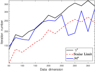
(a) Worst case: $\sigma_{A}=1,\,\,\sigma_{b}=1,\,\,m=5$.

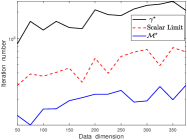
(b) $\sigma_{A}=2,\,\,\sigma_{b}=1/2,\,\,m=5$.

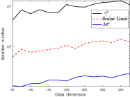
(c) $\sigma_{A}=3,\,\,\sigma_{b}=1/3,\,\,m=5$.

Figure 1: Iteration number complexity against data dimension.

Performance: In Fig. 1(a), the data is generated in the exact same way. In this case, we find that a scalar parameter would (almost) fully exploit the ill-conditioning structure, corresponding to the worst case of our metric-ADMM. In Fig. 1(b), by generating the two types of data $\{\bm{A}_{i}\}_{i=0}^{m}$ and $\{\bm{b}_{i}\}_{i=0}^{m}$ in a ‘reverse’ way, i.e., $\sigma_{A}=1/\sigma_{b}$, we promote a special ill-conditioning structure that cannot be fully exploited by a scalar parameter. In this case, our metric-ADMM shows roughly one order of magnitude advantage. In Fig. 1(c), we promote a stronger ill-conditioning structure, and the advantage increases to roughly two orders of magnitudes. When we further increase the ill-conditioning, the advantage also further increases (the extra experiments are omitted due to limited space). In all cases, we observe that the metric-ADMM has similar performances, with iteration number roughly at $200$, and increases very slowly as the dimension increases, implying a scalable solver is obtained.

7.2 Boolean QP

In this section, we consider the Boolean quadratic program problem. The problem data is fully characterized by $\bm{A}_{0}$ and $\bm{b}_{0}$.

7.2.1 Natural ill-conditioning

For BQP, we note that there exists a natural ill-conditioning structure (that cannot be fully exploited via a scalar parameter), appears related to requiring the underlying solution being integers.

Data setting: We generate the BQP data in the following manner: (i) Randomly generate an integer vector $\bm{x}_{0}$ with entries being either $1$ or $-1$. To achieve this, we first randomly generate its elements via $\mathcal{N}(-0.5,1)$ and then take the sign operation element-wisely (restart if a zero element arises). (ii) Randomly generate elements of matrix $\bm{A}_{0}$ via $\mathcal{N}(0,1)$. (iii) Set $\bm{b}_{0}=\bm{A}_{0}\bm{x}_{0}+\epsilon$, with noise $\epsilon$ randomly generate via $\mathcal{N}(0,0.1)$.

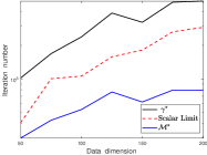
(a) Scalability.

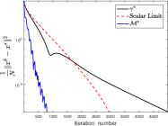
(b) Error decreasing rate, with $N=200$

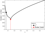
(c) Scalar limit search.

Figure 2: Iteration number complexity performance.

Performance: In Figure 2(a), we evaluate the scalability property of our solver, without manually promoting an ill-conditioning structure. We observe a stable, roughly $3\times$ iteration-complexity advantage compared to the scalar limit. In Figure 2(b), we investigate the convergence rates with data size $N=200$. We observe (roughly) linear rates. Particularly, the metric-quipped one significantly outperforms the best scalar parameter, obtained by exhaustive search. In Figure 2(c), we check the exhaustive search process. We observe that the theoretical optimal scalar (minimized a worst-case convergence rate) is close to the scalar case limit, meanwhile the limit is relatively far away from the unit case $\gamma=1$ (implying the necessity of parameter tuning), and changes with different data sizes (in our additionally experiments).

8 Conclusion

In this paper, we present the first metric-equipped ADMM for semidefinite programming with a worst-case performance guarantee. Equipping a metric parameter is new, owing to the challenges: (i) ADMM $\bm{Z}$-iterate (which handles the positive semidefinite constraint) no longer admits a closed-form expression; (ii) the optimal choice is open. We addressed these two issues in this paper. Additionally, we analyse the worst case of our metric-ADMM. In theory, the worst case corresponds to when the optimal metric reduces to an optimal scalar. Moreover, we identify the data structure that causes it. In practice, the worst case can be interpreted as simple-structured data, i.e., all data generated in the exact same way. Numerically, we observe limited advantage in the worst case compared to employing a scalar parameter, but gains rapidly increased extra efficiency as the conditioning becomes worse. Across all different settings, our metric-based solver shares similar performances (implying the underlying ill-conditioning structure fully exploited), and the iteration number increases very slowly with data dimension.

References

• [1] Lieven Vandenberghe and Stephen Boyd. Semidefinite programming. SIAM review, 38(1):49–95, 1996.
• [2] Stephen Boyd, Laurent El Ghaoui, Eric Feron, and Venkataramanan Balakrishnan. Linear matrix inequalities in system and control theory. SIAM, 1994.
• [3] Lieven Vandenberghe and Stephen Boyd. A primal—dual potential reduction method for problems involving matrix inequalities. Mathematical programming, 69(1-3):205–236, 1995.
• [4] A Kamath and N Karmarkar. A continuous approach to compute upper bounds in quadratic maximization problems with integer constraints. In Recent Advances in Global Optimization, pages 125–140. 1992.
• [5] Anil P Kamath and Narendra K Karmarkar. An o (nl) iteration algorithm for computing bounds in quadratic optimization problems. In Complexity in Numerical Optimization, pages 254–268. World Scientific, 1993.
• [6] Narendra Karmarkar. A new polynomial-time algorithm for linear programming. In Proceedings of the sixteenth annual ACM symposium on Theory of computing, pages 302–311, 1984.
• [7] Yurii Nesterov and A Nemirovsky. A general approach to polynomial-time algorithms design for convex programming. Report, Central Economical and Mathematical Institute, USSR Academy of Sciences, Moscow, 182, 1988.
• [8] Yurii E Nesterov and Arkadii S Nemirovskii. Optimization over positive semidefinite matrices: Mathematical background and user’s manual. USSR Acad. Sci. Centr. Econ. & Math. Inst, 32, 1990.
• [9] Yu Nesterov and Arkadi Nemirovsky. Conic formulation of a convex programming problem and duality. Optimization Methods and Software, 1(2):95–115, 1992.
• [10] Yurii Nesterov and Arkadii Nemirovskii. Interior-point polynomial algorithms in convex programming. SIAM, 1994.
• [11] Michael Grant and Stephen Boyd. CVX: Matlab software for disciplined convex programming, version 2.1, 2014.
• [12] Mosek ApS. Mosek optimization toolbox for matlab. User’s Guide and Reference Manual, Version, 4:1, 2019.
• [13] Amir Beck. First-order methods in optimization. SIAM, 2017.
• [14] Marc Teboulle. A simplified view of first order methods for optimization. Mathematical Programming, 170(1):67–96, 2018.
• [15] Stephen Boyd, Neal Parikh, Eric Chu, Borja Peleato, Jonathan Eckstein, et al. Distributed optimization and statistical learning via the alternating direction method of multipliers. Foundations and Trends® in Machine learning, 3(1):1–122, 2011.
• [16] Roland Glowinski and Americo Marroco. Sur l’approximation, par éléments finis d’ordre un, et la résolution, par pénalisation-dualité d’une classe de problèmes de dirichlet non linéaires. Revue française d’automatique, informatique, recherche opérationnelle. Analyse numérique, 9(R2):41–76, 1975.
• [17] Daniel Gabay and Bertrand Mercier. A dual algorithm for the solution of nonlinear variational problems via finite element approximation. Computers & mathematics with applications, 2(1):17–40, 1976.
• [18] Pierre-Louis Lions and Bertrand Mercier. Splitting algorithms for the sum of two nonlinear operators. SIAM Journal on Numerical Analysis, 16(6):964–979, 1979.
• [19] Jim Douglas and Henry H Rachford. On the numerical solution of heat conduction problems in two and three space variables. Transactions of the American mathematical Society, 82(2):421–439, 1956.
• [20] Donald W Peaceman and Henry H Rachford, Jr. The numerical solution of parabolic and elliptic differential equations. Journal of the Society for industrial and Applied Mathematics, 3(1):28–41, 1955.
• [21] Jonathan Eckstein and Dimitri P Bertsekas. On the Douglas—Rachford splitting method and the proximal point algorithm for maximal monotone operators. Mathematical Programming, 55(1):293–318, 1992.
• [22] Heinz H Bauschke and Patrick L Combettes. Convex Analysis and Monotone Operator Theory in Hilbert Spaces. Springer, 2017.
• [23] Ernest K Ryu and Wotao Yin. Large-scale convex optimization: algorithms & analyses via monotone operators. Cambridge University Press, 2022.
• [24] Yifan Ran. Equilibrate parametrization: Optimal metric selection with provable one-iteration convergence for $l\_1$-minimization. arXiv preprint arXiv:2311.11380, 2023.
• [25] Antonin Chambolle and Thomas Pock. A first-order primal-dual algorithm for convex problems with applications to imaging. Journal of mathematical imaging and vision, 40(1):120–145, 2011.
• [26] Ernie Esser, Xiaoqun Zhang, and Tony F Chan. A general framework for a class of first order primal-dual algorithms for convex optimization in imaging science. SIAM Journal on Imaging Sciences, 3(4):1015–1046, 2010.
• [27] Thomas Pock, Daniel Cremers, Horst Bischof, and Antonin Chambolle. An algorithm for minimizing the Mumford-Shah functional. In 2009 IEEE 12th International Conference on Computer Vision, pages 1133–1140. IEEE, 2009.
• [28] Daniel O’Connor and Lieven Vandenberghe. On the equivalence of the primal-dual hybrid gradient method and Douglas–Rachford splitting. Mathematical Programming, 179(1):85–108, 2020.
• [29] Samuel Burer and Renato DC Monteiro. A nonlinear programming algorithm for solving semidefinite programs via low-rank factorization. Mathematical programming, 95(2):329–357, 2003.
• [30] Samuel Burer and Renato DC Monteiro. Local minima and convergence in low-rank semidefinite programming. Mathematical programming, 103(3):427–444, 2005.
• [31] Yifei Wang, Kangkang Deng, Haoyang Liu, and Zaiwen Wen. A decomposition augmented lagrangian method for low-rank semidefinite programming. SIAM Journal on Optimization, 33(3):1361–1390, 2023.
• [32] Defeng Sun and Jie Sun. Semismooth matrix-valued functions. Mathematics of Operations Research, 27(1):150–169, 2002.
• [33] Xin-Yuan Zhao, Defeng Sun, and Kim-Chuan Toh. A newton-cg augmented lagrangian method for semidefinite programming. SIAM Journal on Optimization, 20(4):1737–1765, 2010.
• [34] Zaiwen Wen, Donald Goldfarb, and Wotao Yin. Alternating direction augmented lagrangian methods for semidefinite programming. Mathematical Programming Computation, 2(3-4):203–230, 2010.
• [35] Bartolomeo Stellato, Goran Banjac, Paul Goulart, Alberto Bemporad, and Stephen Boyd. Osqp: An operator splitting solver for quadratic programs. Mathematical Programming Computation, 12(4):637–672, 2020.
• [36] Yifan Ran. General optimal step-size and initializations for admm: A proximal operator view. arXiv preprint arXiv:2309.10124, 2023.
• [37] Zhi-Quan Luo, Wing-Kin Ma, Anthony Man-Cho So, Yinyu Ye, and Shuzhong Zhang. Semidefinite relaxation of quadratic optimization problems. IEEE Signal Processing Magazine, 27(3):20–34, 2010.
• [38] Stephen P Boyd and Lieven Vandenberghe. Convex optimization. Cambridge university press, 2004.
• [39] Yifan Ran and Wei Dai. Fast and robust admm for blind super-resolution. In ICASSP 2021-2021 IEEE International Conference on Acoustics, Speech and Signal Processing (ICASSP), pages 5150–5154. IEEE, 2021.
• [40] Jonathan Eckstein. Splitting methods for monotone operators with applications to parallel optimization. PhD thesis, Massachusetts Institute of Technology, 1989.
• [41] Isaac. Is there a general formula for solving quartic (degree $4$) equations? Mathematics Stack Exchange. URL:https://math.stackexchange.com/q/786 (version: 2021-12-04).
• [42] Miguel Sousa Lobo, Lieven Vandenberghe, Stephen Boyd, and Hervé Lebret. Applications of second-order cone programming. Linear algebra and its applications, 284(1-3):193–228, 1998.