Discrete Painlevé equations and pencils of quadrics in $\mathbb{P}^{3}$

Abstract. Discrete Painlevé equations constitute a famous class of integrable non-autonomous second order difference equations. A classification scheme proposed by Sakai interprets a discrete Painlevé equation as a birational map between generalized Halphen surfaces (surfaces obtained from $\mathbb{P}^{1}\times\mathbb{P}^{1}$ by blowing up at eight points). Sakai’s classification is thus based on the classification of generalized Halphen surfaces. We propose a novel geometric interpretation of discrete Painlevé equations, where the family of generalized Halphen surfaces is replaced by a pencil of quadrics in $\mathbb{P}^{3}$. A discrete Painlevé equation is viewed as a birational transformation of $\mathbb{P}^{3}$ that preserves the pencil and maps each quadric of the pencil to a different one, according to a Möbius transformation of the pencil parameter. Thus, our scheme is based on the classification of pencils of quadrics in $\mathbb{P}^{3}$.

While historically discrete Painlevé equations appeared as de-autonomizations of QRT maps, in our scheme they are viewed as deformations of 3D QRT maps introduced in our previous paper. A 3D QRT map is defined geometrically as a composition of involutions along generators of quadrics of a pencil, preserving the intersection curves with a second pencil of quadrics. The base set of the net of quadrics spanned by both pencils consists of eight points (which play the role of the eight blow-up points of generalized Halphen surfaces). A Painlevé deformation of a 3D QRT map is obtained by composing involutions along generators with a birational (often linear) transformation of $\mathbb{P}^{3}$ under which the pencil remains invariant, but the individual quadrics are mapped according to a Möbius transformation of the pencil parameter.

1 Introduction

Discrete Painlevé equations belong to the central objects of interest in the theory of discrete integrable systems. Recall that continuous time Painlevé equations are second order nonlinear non-autonomous differential equations with the Painlevé property, which is the absence of moving singularities of solutions other than poles. Grammaticos, Ramani et. al. proposed a discrete version of the latter property called “singularity confinement”, and found the first examples of second order nonlinear non-autonomous difference equations with this property, denoted by them as discrete Painlevé equations [10, 18]. There followed a burst of activity on the subject summarized in [9]. A general classification scheme of discrete Painlevé equations was proposed by Sakai [20], and it is given a detailed exposition in the review paper by Kajiwara, Noumi and Yamada [13]. A monographic account of discrete Painlevé equations is given by Joshi [12].

In the framework of Sakai’s scheme, discrete Painlevé equations are birational maps between generalized Halphen surfaces $X$. The latter can be realized as ${\mathbb{P}}^{1}\times{\mathbb{P}}^{1}$ blown up at eight points with the property that the anti-canonical divisor class $-K_{X}=2H_{1}+2H_{2}-\sum_{i=1}^{8}E_{i}$ contains an effective divisor $D$ admitting a decomposition $D=\sum_{j=1}^{m}D_{j}$ of a canonical type, where $D_{j}$ are irreducible effective divisors with

$$[D_{j}]\cdot[D_{j}]=-2,\quad[D]\cdot[D_{j}]=0,\quad j=1,\ldots,m.$$

Here $H_{1}$ and $H_{2}$ are the divisor classes of proper transforms of a generic vertical, resp. horizontal lines in ${\mathbb{P}}^{1}\times{\mathbb{P}}^{1}$, while $E_{i}$ is the total transform of the $i$-th blow-up. The scalar product in the Picard lattice ${\rm Pic}(X)={\mathbb{Z}}H_{1}+{\mathbb{Z}}H_{2}+\sum_{i=1}^{8}{\mathbb{Z}}E_{i}$ is given by the intersection number:

$$H_{1}\cdot H_{2}=1,\quad E_{i}\cdot E_{i}=-1$$

(all other scalar products among generators vanish). The matrix $([D_{i}]\cdot[D_{j}])_{i,j=1}^{m}$ is the (negative of the) Cartan matrix of an affine root system $R(X)$, called the surface type of $X$. In particular, if $m=1$, so that the anti-canonical divisor class only contains irreducible effective divisors (irreducible curves of bidegree (2,2) in ${\mathbb{P}}^{1}\times{\mathbb{P}}^{1}$ passing through all eight blow-up points), one speaks about the surface type $A_{0}^{(1)}$.

Since the early days of the theory, discrete Painlevé equations were considered as non-autonomous versions (or modifications) of the so called QRT maps [15, 16], [8]. The latter are birational maps of ${\mathbb{P}}^{1}\times{\mathbb{P}}^{1}$ defined as compositions of a vertical and a horizontal involutions generated by a pencil of biquadratic curves. While in the old-style literature the non-autonomous modification was mainly introduced in an ad hoc way by allowing some coefficients of the map to become time-dependent, a more geometric version of this procedure was proposed in the framework of the Sakai’s scheme by Carstea, Dzhamay and Takenawa [4]. In their scheme, the de-automization of a given QRT map depends on the choice of one biquadratic curve of the pencil.

In the present paper, we propose an alternative view on discrete Painlevé equations, and simultaneously an alternative procedure for the de-autonomization of QRT maps. In our scheme, the surfaces on which discrete Painlevé equations act are quadrics of a pencil in ${\mathbb{P}}^{3}$. Our scheme can be described as follows.

1. Start with a pencil $\{C_{\mu}\}$ of biquadratic curves in ${\mathbb{P}}^{1}\times{\mathbb{P}}^{1}$ and the corresponding QRT map. Let $s_{1},\ldots,s_{8}\in{\mathbb{P}}^{1}\times{\mathbb{P}}^{1}$ be the base points of this pencil. Lift $\{C_{\mu}\}$ to a pencil of quadrics $\{P_{\mu}\}$ in ${\mathbb{P}}^{3}$. The base curve of this pencil passes through the lifts $S_{1},\ldots,S_{8}$ of the base points $s_{1},\ldots,s_{8}$.

2. Choose one distinguished biquadratic curve $C_{\infty}$ of the pencil, along with its lift to a quadric $P_{\infty}$.

3. Based on these data, construct the pencil of quadrics $\{Q_{\lambda}\}$ in ${\mathbb{P}}^{3}$ spanned by $Q_{0}=\{X_{1}X_{2}-X_{3}X_{4}=0\}$ and by $P_{\infty}$. Recall that $Q_{0}$ is nothing but the Segre embedding of ${\mathbb{P}}^{1}\times{\mathbb{P}}^{1}$ to ${\mathbb{P}}^{3}$. The base curve of the pencil $\{Q_{\lambda}\}$ is, by definition, the curve $Q_{0}\cap P_{\infty}$, which is the image of $C_{\infty}$ under the Segre embedding. The intersection of this curve with the base curve of the pencil $\{P_{\mu}\}$ consists exactly of the points $S_{1},\ldots,S_{8}$.

4. Consider a 3D QRT map on the pencil $\{Q_{\lambda}\}$ defined by intersections of its generators with the quadrics $P_{\mu}$. Recall that the notion of 3D QRT maps was introduced in [1] and that such a map preserves each quadric $Q_{\lambda}$ (and therefore the pencil parameter $\lambda$ serves as an integral of motion). On each quadric $Q_{\lambda}$, our map induces a QRT map which can be considered as a $\lambda$-deformation of the original QRT map.

5. Consider a birational map $L$ on ${\mathbb{P}}^{3}$ with the following properties.

   • $L$ preserves the pencil $\{Q_{\lambda}\}$ and its base curve, and maps each $Q_{\lambda}$ to $Q_{\sigma(\lambda)}$, where $\sigma:{\mathbb{P}}^{1}\to{\mathbb{P}}^{1}$ is a Möbius automorphism fixing the set

     $${\rm Sing}(Q):=\big{\{}\lambda\in{\mathbb{P}}^{1}:\;Q_{\lambda}\;{\rm is\;\;degenerate}\big{\}}.$$ (1)

   • The maps $L\circ i_{1},L\circ i_{2}$ have the same singularity confinement properties as the QRT involutions $i_{1},i_{2}$.

   Then the map $(L\circ i_{1})\circ(L\circ i_{2})$ is declared to be a discrete Painlevé equation obtained by the de-autonomization of the QRT map along the fiber $C_{\infty}$.

The structure of the paper is as follows. We start by recalling several general concepts necessary for our presentation, namely the notion of singularity confinement for birational maps (Section 2), construction and basic properties of QRT maps (Section 3), a three-dimensional generalization of QRT maps introduced in [1] (Section 4), as well as a classical projective classification of pencil of quadrics in $\mathbb{P}^{3}$ (Section 5). Then, in Section 6, we describe in detail the points 3 and 4 of the scheme above, i.e., a construction of a 3D QRT map based on the choice of a biquadratic curve in the invariant fibration of a given QRT map. Finally, the general part culminates in the discussion of the notion of the Painlevé deformation in Section 7. There follow seven Sections 8–14 contaning a detailed elaboration of our scheme for seven (out of thirteen) projective classes of pencils of quadrics. These cases are characterized by the property that the characteristic polynomial of the pencil is a complete square, and, as a consequence, the generators of the pencil are rational functions on $\mathbb{P}^{3}$.

In the present form, our scheme covers discrete Painlevé equations of the Sakai’s scheme for all surface types below $A_{0}^{(1)}$. It does include a multiplicative and additive versions of $A_{1}^{(1)}$ (Sections 13, 14), however in a realization different from the one in [13]. Namely, in our realization the roots are $[D_{1}]=2H_{1}+H_{2}-\sum_{i=1}^{6}E_{i}$ and $[D_{2}]=H_{2}-E_{7}-E_{8}$, i.e., $D_{1}$ corresponds to a curve of bidegree (2,1) through six blow-up points and $D_{2}$ corresponds to a horizontal line through two blow-up points. Recall that in the realization in [13] the roots are $[D_{1}]=H_{1}+H_{2}-\sum_{i=1}^{4}E_{i}$ and $[D_{2}]=H_{1}+H_{2}-\sum_{i=5}^{8}E_{i}$, i.e., $D_{1}$ and $D_{2}$ correspond to two curves of bidegree (1,1) through four blow-up points each.

Modifications of our scheme necessary to treat the remaining six cases (the multiplicative and the additive discrete Painlevé equations of the type $A_{1}^{(1)}$ in the latter realization, as well as the elliptic, the multiplicative and the additive equations of the type $A_{0}^{(1)}$) will be discussed in a subsequent paper [2].

Acknowledgement.

This research is supported by the DFG Collaborative Research Center TRR 109 “Discretization in Geometry and Dynamics”.

2 Generalities: singularity confinement

For birational maps of $\mathbb{P}^{N}$, we will use the following basic notions and results [11], [6], [7]. Let such a map $f:\mathbb{P}^{N}\dasharrow\mathbb{P}^{N}$ be given by $N+1$ homogeneous polynomials of one and the same degree $d$ without a non-trivial common factor,

$$f:\;[x_{0}:x_{1}:\ldots:x_{N}]\mapsto[X_{0}:X_{1}:\ldots:X_{N}].$$ (2)

The number $d$ is called the degree of $f$, denoted by $\deg(f)$. The corresponding polynomial map of $\mathbb{C}^{N+1}$ will be denoted by $\tilde{f}$ and will be called a minimal lift of $f$. It is defined up to a constant factor. To each birational map we associate:

• the indeterminacy set $\mathcal{I}(f)$ consisting of the points $[x_{0}:x_{1}:\ldots:x_{N}]\in\mathbb{P}^{N}$ for which $X_{0}=X_{1}=\ldots=X_{N}=0$; this is a variety of codimension at least 2;

• the critical set $\mathcal{C}(f)$ consisting of the points $[x_{0}:x_{1}:\ldots:x_{N}]\in\mathbb{P}^{N}$ where $\det d\tilde{f}=0$; the latter equation of degree $(N+1)(d-1)$ defines a variety of codimension 1.

There holds $\mathcal{I}(f)\subset\mathcal{C}(f)$. Away from $\mathcal{C}(f)$, the map $f$ acts biregularly. On the other hand, the image of $\mathcal{C}(f)\setminus\mathcal{I}(f)$ under the map $f$ belongs to $\mathcal{I}(f^{-1})$ (in particular, it is of codimension $\geq 2$). Loosely speaking, $f$ contracts (or blows down) hypersurfaces from $\mathcal{C}(f)$.

The further fate of the images of $\mathcal{C}(f)$ under iterates of $f$ is essential for the notion of singularity confinement. This notion was originally introduced in [10] as an integrability criterium, see its current status in [14]. An algebro-geometric interpretation of singularity confinement, which we adopt below, followed in [3], where it was shown to be related to the phenomenon of the drop of degree of iterates $f^{k}$, which in turn is responsible for the drop of the dynamical degree of $f$. The drop of degree of $f^{k}$ happens if in all components of the polynomial map $\tilde{f}^{k}$ there appears a common polynomial factor. A geometric condition for this is the existence of degree lowering hypersurfaces.

Definition 1

A hypersurface $A=\{a=0\}\subset\mathcal{C}(f)$ (where $a(x_{0},x_{1},\ldots,x_{N})$ is a homogeneous polynomial on $\mathbb{C}^{N+1}$) is called a degree lowering hypersurface for the map $f$ if $f^{k-1}(A)\subset\mathcal{I}(f)$ for some $k\in\mathbb{N}$.

Indeed, in this case all components of $\tilde{f}^{k}$ vanish as soon as $a=0$, and therefore are divisible by $a$. As a corollary, the dynamical degree of the map $f$, defined as

$$\lambda(f):=\lim_{n\to\infty}(\deg(f^{n}))^{1/n},$$ (3)

is strictly less than $\deg f$. The condition $\lambda(f)=1$, or, equivalently, the vanishing of the algebraic entropy $h(f)=\log\lambda(f)$, is a popular definition of integrability of a birational map $f$ (cf. [3]). In particular, one often refers to this definition (or criterium) when speaking about discrete Painlevé equations [12], [13].

For a degree lowering hypersurface $A\subset\mathcal{C}(f)$, with $f^{k}(A)\subset\mathcal{I}(f)$, we call the diagram

$$A\stackrel{{\scriptstyle f}}{{\to}}f(A)\stackrel{{\scriptstyle f}}{{\to}}f^{2}(A)\stackrel{{\scriptstyle f}}{{\to}}\ldots\stackrel{{\scriptstyle f}}{{\to}}f^{k}(A)\stackrel{{\scriptstyle f}}{{\to}}B$$ (4)

a singularity confinement pattern. In such a pattern, one should think of $f$ as blowing up $f^{k}(A)\subset\mathcal{I}(f)$ to a hypersurface $B\subset\mathcal{C}(f^{-1})$. In the present paper, we will not address the issue of regularizing the map $f$, i.e., lifting it to a blow-up variety $X$ so that the lift is algebraically stable (does not possess degree lowering hypersurfaces). According to a theorem by Diller and Favre [7], this is always possible in dimension $N=2$. For a map with an algebraically stable lift, the dynamical degree $\lambda(f)$ can be computed as the spectral radius of the induced action of this lift on the Picard group ${\rm Pic}(X)$. All our examples here (in dimensions $N=2$ and $N=3$) possess algebraically stable lifts, moreover, all singularities are confined in the sense that all components of the critical set are degree lowering, resulting in singularity confinement patterns as in (4).

3 Generalities: QRT maps

To quickly introduce QRT maps, consider a pencil of biquadratic curves

$$C_{\mu}=\Big{\{}(x,y)\in{\mathbb{C}}^{2}:C_{\mu}(x,y):=C_{0}(x,y)-\mu C_{\infty}(x,y)=0\Big{\}},$$

where $C_{0},C_{\infty}$ are two polynomials of bidegree (2,2). The base set $\mathcal{B}$ of the pencil is defined as the set of points through which all curves of the pencil pass or, equivalently, as the intersection $\{C_{0}(x,y)=0\}\cap\{C_{\infty}(x,y)=0\}$. Through any point $(x_{0},y_{0})\not\in\mathcal{B}$, there passes exactly one curve of the pencil, defined by $\mu=\mu(x_{0},y_{0})=C_{0}(x_{0},y_{0})/C_{\infty}(x_{0},y_{0})$. Actually, we consider this pencil in a compactification ${\mathbb{P}}^{1}\times{\mathbb{P}}^{1}$ of ${\mathbb{C}}^{2}$. Then, $B$ consists of eight base points, counted with multiplicity, $\mathcal{B}=\{s_{1},\ldots,s_{8}\}\subset{\mathbb{P}}^{1}\times{\mathbb{P}}^{1}$.

One defines the vertical switch $i_{1}$ and the horizontal switch $i_{2}$ as follows. For a given point $(x_{0},y_{0})\in{\mathbb{P}}^{1}\times{\mathbb{P}}^{1}\setminus\mathcal{B}$, determine $\mu=\mu(x_{0},y_{0})$ as above. Then the vertical line $\{x=x_{0}\}$ intersects $C_{\mu}$ at exactly one further point $(x_{0},y_{1})$ which is defined to be $i_{1}(x_{0},y_{0})$; similarly, the horizontal line $\{y=y_{0}\}$ intersects $C_{\mu}$ at exactly one further point $(x_{1},y_{0})$ which is defined to be $i_{2}(x_{0},y_{0})$. The QRT map is defined as

$$f=i_{1}\circ i_{2}.$$

Each of the maps $i_{1}$, $i_{2}$ is a birational involution on ${\mathbb{P}}^{1}\times{\mathbb{P}}^{1}$ with indeterminacy set $\mathcal{B}$. Likewise, the QRT map $f$ is a (dynamically nontrivial) birational map on ${\mathbb{P}}^{1}\times{\mathbb{P}}^{1}$, having $\mu(x,y)=C_{0}(x,y)/C_{\infty}(x,y)$ as an integral of motion. A generic fiber $C_{\mu}$ is an elliptic curve, and $f$ acts on it as a shift with respect to the corresponding addition law.

We briefly discuss singularity confinement patterns for QRT maps.

• If a base point $s_{i}=(a_{i},b_{i})$ is the only base point on the line $\{x=a_{i}\}$ and the only base point on the line $\{y=b_{i}\}$, then it is an indeterminacy point for both involutions $i_{1}$, $i_{2}$. More precisely, $i_{1}$ blows down the line $\{x=a_{i}\}$ to the point $s_{i}$ (and, since it is an involution, blows up the point $s_{i}$ to the line $\{x=a_{i}\}$). Likewise, $i_{2}$ blows down the line $\{y=b_{i}\}$ to the point $s_{i}$ and blows up the point $s_{i}$ to the line $\{y=b_{i}\}$. We say that the following short singularity confinement pattern for the involutions $i_{1}$, $i_{2}$ happens:

  $$\{x=a_{i}\}\;\stackrel{{\scriptstyle i_{1}}}{{\rightarrow}}\;s_{i}\;\stackrel{{\scriptstyle i_{2}}}{{\rightarrow}}\;\{y=b_{i}\}.$$ (5)

  As a consequence, we have also a short singularity confinement pattern for the map $f=i_{1}\circ i_{2}$:

  $$i_{2}(\{x=a_{i}\}\;\stackrel{{\scriptstyle f}}{{\rightarrow}}\;s_{i}\;\stackrel{{\scriptstyle f}}{{\rightarrow}}\;i_{1}(\{y=b_{i}\}).$$ (6)

• If there are two base points $s_{i}=(a_{i},b_{i})$ and $s_{j}=(a_{i},b_{j})$ on the line $\{x=a_{i}\}$, then both are singularities for the involution $i_{2}$, being blown up to the corresponding lines $\{y=b_{i}\}$, resp. $\{y=b_{j}\}$. On the contrary, for the involution $i_{1}$ the line $\{x=a_{i}\}$ is invariant; $i_{1}$ induces a projective (Möbius) involution on this line, which interchanges the points $s_{i}$ and $s_{j}$. We say that the following long singularity confinement patterns for the involutions $i_{1}$, $i_{2}$ happen:

  $$\{y=b_{i}\}\;\stackrel{{\scriptstyle i_{2}}}{{\rightarrow}}\;s_{i}\;\stackrel{{\scriptstyle i_{1}}}{{\rightarrow}}\;s_{j}\;\stackrel{{\scriptstyle i_{2}}}{{\rightarrow}}\;\{y=b_{j}\}$$ (7)

  (and a similar one with the roles of $s_{i}$ and $s_{j}$ interchanged). As a consequence, we have also short singularity confinement patterns for the map $f=i_{1}\circ i_{2}$:

  $$\{y=b_{i}\}\;\stackrel{{\scriptstyle f}}{{\rightarrow}}\;s_{j}\;\stackrel{{\scriptstyle f}}{{\rightarrow}}\;i_{1}(\{y=b_{j}\})$$ (8)

  (and a similar one involving $s_{i}$).

• Analogously, if there are two base points $s_{i}=(a_{i},b_{i})$ and $s_{j}=(a_{j},b_{i})$ on the line $\{y=b_{i}\}$, then both are singularities for the involution $i_{1}$, being blown up to the corresponding lines $\{x=a_{i}\}$, resp. $\{x=a_{j}\}$. For the involution $i_{2}$ the line $\{y=b_{i}\}$ is invariant; it induces a projective (Möbius) involution on this line, which interchanges the points $s_{i}$ and $s_{j}$. A long singularity confinement pattern happens for the involutions $i_{1}$, $i_{2}$:

  $$\{x=a_{i}\}\;\stackrel{{\scriptstyle i_{1}}}{{\rightarrow}}\;s_{i}\;\stackrel{{\scriptstyle i_{2}}}{{\rightarrow}}\;s_{j}\;\stackrel{{\scriptstyle i_{1}}}{{\rightarrow}}\;\{x=a_{j}\}$$ (9)

  (and a similar one with the roles of $s_{i}$ and $s_{j}$ interchanged). As a consequence, a short singularity confinement pattern happens for the map $f=i_{1}\circ i_{2}$:

  $$i_{2}(\{x=a_{i}\})\;\stackrel{{\scriptstyle f}}{{\rightarrow}}\;s_{i}\;\stackrel{{\scriptstyle f}}{{\rightarrow}}\;\{x=a_{j}\}$$ (10)

  (and a similar one involving $s_{j}$).

Summarizing, for the map $f$ there are eight short singularity confinement patterns, each of the base points participating in exactly one pattern. For the involutions $i_{1}$, $i_{2}$ one also has eight singularity confinement patterns, but some of them become long if the base points are in a special relative position. Of course, further degenerations are possible in case of further geometric specialties in the configuration of the base points, e.g., if there are infinitely near points among them.

4 Generalities: three-dimensional QRT maps

On the way towards a 3D generalization of QRT maps, the first step is a translation of the construction just described to a Segre embedding of ${\mathbb{P}}^{1}\times{\mathbb{P}}^{1}$ as a quadric in ${\mathbb{P}}^{3}$:

$$Q_{0}=\Big{\{}[X_{1}:X_{2}:X_{3}:X_{4}]:X_{1}X_{2}-X_{3}X_{4}=0\Big{\}}\subset{\mathbb{P}}^{3}.$$ (11)

Thus, $Q_{0}$ is isomorphic to ${\mathbb{P}}^{1}\times{\mathbb{P}}^{1}$, via the Segre embedding

$$\phi_{0}:\quad{\mathbb{P}}^{1}\times{\mathbb{P}}^{1}\ni\big{(}[x_{1}:x_{0}],[y_{1}:y_{0}]\big{)}\,\mapsto\;[x_{1}y_{0}:x_{0}y_{1}:x_{1}y_{1}:x_{0}y_{0}]\in Q_{0}.$$ (12)

Usually, we write this in the affine chart ${\mathbb{C}}\times{\mathbb{C}}$ of ${\mathbb{P}}^{1}\times{\mathbb{P}}^{1}$ as follows:

$$\phi_{0}:\quad{\mathbb{P}}^{1}\times{\mathbb{P}}^{1}\ni(x,y)\,\mapsto\;[x:y:xy:1]\in Q_{0}.$$ (13)

The quadric $Q_{0}$, like any non-degenerate quadric in ${\mathbb{P}}^{3}$, admits two rulings such that any two lines of one ruling are skew and any line of one ruling intersects any line of the other ruling. Through each point $X\in Q_{0}$ there pass two straight lines, one of each of the two rulings, let us call them $\ell_{1}(X)$ and $\ell_{2}(X)$. More concretely, $\ell_{1}(X)$ can be described as $\{x={\rm const}\}$, while $\ell_{2}(X)$ can be described as $\{y={\rm const}\}$.

Now, any biquadratic curve in ${\mathbb{P}}^{1}\times{\mathbb{P}}^{1}$ with the equation

$$C:\;\big{\{}a_{1}x^{2}y^{2}+a_{2}x^{2}y+a_{3}xy^{2}+a_{4}x^{2}+a_{5}y^{2}+a_{6}xy+a_{7}x+a_{8}y+a_{9}=0\big{\}}$$

can be identified with $Q_{0}\cap P$, where $P$ is the quadric in $\mathbb{P}^{3}$ with the equation

$$P:\;\big{\{}a_{1}X_{3}^{2}+a_{2}X_{1}X_{3}+a_{3}X_{2}X_{3}+a_{4}X_{1}^{2}+a_{5}X_{2}^{2}+a_{6}X_{3}X_{4}+a_{7}X_{1}X_{4}+a_{8}X_{2}X_{4}+a_{9}X_{4}^{2}=0\big{\}}.$$

Therefore, a pencil of biquadratic curves $\{C_{\mu}\}$ in ${\mathbb{P}}^{1}\times{\mathbb{P}}^{1}$ can be identified with intersections of $Q_{0}$ with a pencil of quadrics $\{P_{\mu}\}$ in ${\mathbb{P}}^{3}$. The corresponding QRT map can be identified with $f=i_{1}\circ i_{2}$, where $i_{1}$, $i_{2}$ are involutions on $Q_{0}$ defined as follows. For a given point $X\in Q_{0}$, let $\mu=\mu(X)$ be defined as the value of the pencil parameter for which $X\in Q_{0}\cap P_{\mu}$. Denote by $i_{1}(X)$, $i_{2}(X)$ the second intersection point of $\ell_{1}(X)$ with $P_{\mu}$, resp. the second intersection point of $\ell_{2}(X)$ with $P_{\mu}$.

Now we are in a position to give a three-dimensional generalization of the QRT construction. For this, consider a second pencil of quadrics $\{Q_{\lambda}\}$ in ${\mathbb{P}}^{3}$, and consider the QRT construction on each fiber $Q_{\lambda}$ individually.

Definition 2

Given two pencils of quadrics $\{Q_{\lambda}\}$ and $\{P_{\mu}\}$, we define birational involutions $i_{1},i_{2}:{\mathbb{P}}^{3}\dasharrow{\mathbb{P}}^{3}$ as follows: for a generic $X\in{\mathbb{P}}^{3}$ (not belonging to the base set of either pencil), determine $\lambda,\mu\in{\mathbb{P}}^{1}$ such that $X\in Q_{\lambda}\cap P_{\mu}$; then $i_{1}(X)$ is defined to be the second intersection point of the generator $\ell_{1}(X)$ of $Q_{\lambda}$ with $P_{\mu}$, and similarly $i_{2}(X)$ is the second intersection point of the generator $\ell_{2}(X)$ of $Q_{\lambda}$ with $P_{\mu}$. The 3D QRT map is defined as $f=i_{1}\circ i_{2}:{\mathbb{P}}^{3}\dasharrow{\mathbb{P}}^{3}$; it leaves all quadrics of both pencils invariant.

The main problem with this definition is that the dependence of generators $\ell_{1}(X)$, $\ell_{2}(X)$ on the point $X$ can be non-rational. This issue is the subject of the following section.

5 Generalities: pencils of quadrics

Let $\{Q_{\lambda}\}_{\lambda\in{\mathbb{P}}^{1}}$ be a pencil of quadrics in ${\mathbb{P}}^{3}$, with $Q_{\lambda}=Q_{0}-\lambda Q_{\infty}$. Denote by $M_{0},M_{\infty}\in{\rm Sym}_{4\times 4}({\mathbb{C}})$ symmetric matrices of the quadratic forms $Q_{0},Q_{\infty}$, and set $M_{\lambda}=M_{0}-\lambda M_{\infty}$.

It is well known (see, e..g., [5]) that pencils of quadrics in ${\mathbb{P}}^{3}$ are classified, modulo complex congruence transformations, by the structure of the system of elementary divisors of $M_{\lambda}$, encoded in the so called Segre symbols. Elementary divisors are powers of $\lambda-\lambda_{k}$ for $\lambda_{k}\in\,{\rm Sing}(Q):=\{\lambda\in{\mathbb{P}}^{1}:Q_{\lambda}\;\;{\rm is\;\;singular}\}$. The product of all elementary divisors is the characteristic polynomial

$$\Delta(\lambda)=\det(M_{\lambda})=\det(M_{0}-\lambda M_{\infty}).$$ (14)

The classification of pencils of quadrics in ${\mathbb{P}}^{3}$ modulo complex congruence transformations consists of the following thirteen classes:

• Pencil of quadrics through a non-singular spatial quartic curve.
  Segre symbol $[1,1,1,1]$; $\Delta(\lambda)=(\lambda-\lambda_{1})(\lambda-\lambda_{2})(\lambda-\lambda_{3})(\lambda-\lambda_{4})$.

• Pencil of quadrics through a nodal spatial quartic curve.
  Segre symbol $[2,1,1]$; $\Delta(\lambda)=(\lambda-\lambda_{1})^{2}(\lambda-\lambda_{2})(\lambda-\lambda_{3})$.

• Pencil of quadrics through a cuspidal spatial quartic curve.
  Segre symbol $[3,1]$; $\Delta(\lambda)=(\lambda-\lambda_{1})^{3}(\lambda-\lambda_{2})$.

• Pencil of quadrics through two non-coplanar conics sharing two points.
  Segre symbol $[(1,1),1,1]$; $\Delta(\lambda)=(\lambda-\lambda_{1})^{2}(\lambda-\lambda_{2})(\lambda-\lambda_{3})$.

• Pencil of quadrics through two non-coplanar conics touching at a point.
  Segre symbol $[(2,1),1]$; $\Delta(\lambda)=(\lambda-\lambda_{1})^{3}(\lambda-\lambda_{2})$.

• Pencil of quadrics tangent along a non-degenerate conic.
  Segre symbol $[(1,1,1),1]$; $\Delta(\lambda)=(\lambda-\lambda_{1})^{3}(\lambda-\lambda_{2})$.

• Pencil of quadrics through a twisted cubic and one of its chords.
  Segre symbol $[2,2]$; $\Delta(\lambda)=(\lambda-\lambda_{1})^{2}(\lambda-\lambda_{2})^{2}$.

• Pencil of quadrics through a twisted cubic and one of its tangents.
  Segre symbol $[4]$; $\Delta(\lambda)=(\lambda-\lambda_{1})^{4}$.

• Pencil of quadrics through a conic and two coplanar lines through different points of the conic.
  Segre symbol $[2,(1,1)]$; $\Delta(\lambda)=(\lambda-\lambda_{1})^{2}(\lambda-\lambda_{2})^{2}$.

• Pencil of quadrics through a conic and two lines meeting on the conic.
  Segre symbol $[(3,1)]$; $\Delta(\lambda)=(\lambda-\lambda_{1})^{4}$.

• Pencil of quadrics through a skew quadrilateral.
  Segre symbol $[(1,1),(1,1)]$; $\Delta(\lambda)=(\lambda-\lambda_{1})^{2}(\lambda-\lambda_{2})^{2}$.

• Pencil of quadrics through three lines, tangent along one of them.
  Segre symbol $[(2,2)]$; $\Delta(\lambda)=(\lambda-\lambda_{1})^{4}$.

• Pencil of quadrics tangent along a pair of lines.
  Segre symbol $[(2,1,1)]$; $\Delta(\lambda)=(\lambda-\lambda_{1})^{4}$.

By a projective (Möbius) transformation of $\lambda$, one can achieve $\lambda_{1}=\infty$, $\lambda_{2}=0$, $\lambda_{3}=1$. In the case (i), we have one module, the cross-ratio of $\lambda_{1},\ldots,\lambda_{4}$. All other cases are exhausted by just one pencil, up to the projective transformations of $\mathbb{P}^{3}$ and Möbius transformations of $\lambda$ (e.g., with the values of $\lambda_{i}$ just mentioned).

Consider the following problem. Suppose that $Q_{0}(X)=X_{1}X_{2}-X_{3}X_{4}$. Find a linear projective change of variables $X=A_{\lambda}Y$ reducing the quadratic form $Q_{\lambda}$ to the standard form $Q_{0}$:

$$Q_{\lambda}(A_{\lambda}Y)=Q_{0}(Y),\quad{\rm or}\quad A_{\lambda}^{\rm T}M_{\lambda}A_{\lambda}=M_{0}.$$ (15)

Proposition 1

The normalizing matrix $A_{\lambda}$ is a rational fuction of $\lambda$ and of $\sqrt{\Delta(\lambda)}$. In particular, it is a rational function of $\lambda$ if $\Delta(\lambda)$ is a complete square, i.e., for the seven cases (vii)–(xiii).

As a corollary, we obtain what can be called pencil-adapted coordinates

$$\begin{bmatrix}X_{1}\\ X_{2}\\ X_{3}\\ X_{4}\end{bmatrix}=A_{\lambda}\begin{bmatrix}x\\ y\\ xy\\ 1\end{bmatrix}=:\phi_{\lambda}(x,y).$$ (16)

Thus, $\phi_{\lambda}$ gives a parametrization of $Q_{\lambda}$ by $(x,y)\in{\mathbb{P}}^{1}\times{\mathbb{P}}^{1}$, such that the generators $\ell_{1}$, resp. $\ell_{2}$ of $Q_{\lambda}$ correspond to $x={\rm const}$, resp. to $y={\rm const}$.

This establishes a connection to a particular case of a general result of M. Reid [19, Theorem 1.10] on the structure of the set ${\rm Gen}(Q)$ of generators of a pencil of quadrics $Q=\{Q_{\lambda}\}_{\lambda\in{\mathbb{P}}^{1}}$ in ${\mathbb{P}}^{n}={\mathbb{P}}({\mathbb{C}}^{n+1})$, considered as a subvariety of ${\mathbb{P}}^{1}\times{\rm Gr}([\frac{n+1}{2}],{\mathbb{C}}^{n+1})$. Reid’s theorem says that ${\rm Gen}(Q)$ is a non-singular variety, and for $n$ odd, the first projection ${\rm Gen}(Q)\stackrel{{\scriptstyle p_{1}}}{{\rightarrow}}{\mathbb{P}}^{1}$ factorizes as ${\rm Gen}(Q)\stackrel{{\scriptstyle p}}{{\rightarrow}}C\stackrel{{\scriptstyle q}}{{\rightarrow}}{\mathbb{P}}^{1}$, where $C$ is non-singular, and $q$ is a double covering ramified precisely in ${\rm Sing}(Q)$, and $p$ is smooth. Here, ${\rm Sing}(Q)$ is a finite number of values of $\lambda\in{\mathbb{P}}^{1}$ for which the quadric $Q_{\lambda}$ is degenerate.

In practical terms, in our case $n=3$, we can formulate the following statement.

Proposition 2

For a point $X$ from $Q_{\lambda}$, the generators $\ell_{1}(X)$ and $\ell_{2}(X)$ are rational functions of $X$ and of $\sqrt{\Delta(\lambda)}$. In particular, they are rational functions of $X$ and of $\lambda$ if $\Delta(\lambda)$ is a complete square, i.e., for the seven cases (vii)–(xiii).

6 A 3D QRT map defined by a chosen fiber of the pencil $C_{\mu}$

We now specify the construction of a 3D QRT map from Section 4 by making a special choice of the pencil $Q_{\lambda}$.

$\bullet\,$ In the pencil of biquadratic curves $\{C_{\mu}\}$ in ${\mathbb{P}}^{1}\times{\mathbb{P}}^{1}$, choose a fiber $C_{\infty}$. We will assume that this is the fiber admitting a decomposition of a canonical type; this condition is not necessary for the construction but will facilitate the discussion of singularity confinement below. Take the corresponding quadric $P_{\infty}$ in ${\mathbb{P}}^{3}$, and set

$$Q_{\lambda}=Q_{0}-\lambda P_{\infty}.$$ (17)

Thus, the pencils $\{Q_{\lambda}\}$ and $\{P_{\mu}\}$ have one quadric $P_{\infty}$ in common. The base set of the pencil $\{Q_{\lambda}\}$ is $Q_{0}\cap P_{\infty}=\phi_{0}(C_{\infty})$. Of course, this base set contains the images of the base points $s_{1},\ldots,s_{8}$ of the pencil $\{C_{\mu}\}$ under the Segre embedding:

$$S_{i}=\phi_{0}(s_{i}),\quad i=1,\ldots,8.$$ (18)

The set $\{S_{1},\ldots,S_{8}\}$ can be characterized as the intersection of the base curve of the pencil $\{Q_{\lambda}\}$ with the base curve of the pencil $\{P_{\mu}\}$, or, alternatively, as the base set of a two-parameter linear family (net) of quadrics spanned by $Q_{0}$ and $\{P_{\mu}\}$. Our standing assumption in this paper will be the following.

Assumption. The characteristic polynomial $\Delta(\lambda)$ of the pencil $\{Q_{\lambda}\}$ is a complete square.

Thus, we will be dealing here with the seven cases (vii)–(xiii) of the classification of pencils considered in Section 5. The six cases (i)–(vi) will be dealt with in a follow-up paper [2]

$\bullet\,$ Find a linear change of variables $X=A_{\lambda}Y$ reducing the quadratic form $Q_{\lambda}(X)$ to the standard form $Q_{0}(Y)$, as in (15). The above assumption ensures that $A_{\lambda}$ is a rational function of $\lambda$. This gives the pencil-adapted coordinates

$$\phi_{\lambda}:{\mathbb{P}}^{1}\times{\mathbb{P}}^{1}\to Q_{\lambda},$$

as in (16), which can be understood as a parametrization of $Q_{\lambda}$ by $(x,y)\in{\mathbb{P}}^{1}\times{\mathbb{P}}^{1}$, such that the generators $\ell_{1}$, resp. $\ell_{2}$ of $Q_{\lambda}$ correspond to $x={\rm const}$, resp. to $y={\rm const}$.

$\bullet\,$ Clearly, for each fixed $\lambda$, the intersection curves $Q_{\lambda}\cap P_{\mu}$ in coordinates $(x,y)$ form a pencil of biquadratic curves $\phi_{\lambda}^{*}P_{\mu}$. This pencil can be characterized by its eight base points $s_{1}(\lambda),\ldots,s_{8}(\lambda)\in{\mathbb{P}}^{1}\times{\mathbb{P}}^{1}$ which are nothing else but the points $S_{1},\ldots,S_{8}$ expressed in the coordinates $\phi_{\lambda}$:

$$\phi_{\lambda}(s_{i}(\lambda))=S_{i},\quad i=1,\ldots,8.$$ (19)

An important object is also the curve $C_{\infty}(\lambda)\subset{\mathbb{P}}^{1}\times{\mathbb{P}}^{1}$ which is just the curve $\phi_{0}(C_{\infty})$ expressed in the coordinates $\phi_{\lambda}$:

$$\phi_{\lambda}(C_{\infty}(\lambda))=\phi_{0}(C_{\infty}).$$ (20)

Clearly, the curve $C_{\infty}(\lambda)$ contains the base points $s_{1}(\lambda),\ldots,s_{8}(\lambda)$. Moreover, it admits a decomposition of the canonical type, of the same surface type as $C_{\infty}$.

$\bullet\,$ Construct the involutions $i_{1},i_{2}:{\mathbb{P}}^{3}\dasharrow{\mathbb{P}}^{3}$ along generators of the pencil $\{Q_{\lambda}\}$ till the second intersection with $\{P_{\mu}\}$, and the 3D QRT map $f=i_{1}\circ i_{2}:{\mathbb{P}}^{3}\dasharrow{\mathbb{P}}^{3}$, as described in Definition 2. Note that the above assumption ensures that all these maps are birational. One possibility for an effective computing of these maps is to first compute the restrictions $i_{1}|_{Q_{\lambda}}$ and $i_{2}|_{Q_{\lambda}}$ as the QRT switches corresponding to the pencil $\phi_{\lambda}^{*}P_{\mu}$, and then to push them to homogeneous coordinates $X$ on ${\mathbb{P}}^{3}$ using (16) along with $\lambda=Q_{0}(X)/P_{\infty}(X)$.

It is important to observe that the singularity confinement properties of $i_{1}|_{Q_{\lambda}}$, $i_{2}|_{Q_{\lambda}}$ and of $f|_{Q_{\lambda}}=i_{1}|_{Q_{\lambda}}\circ i_{2}|_{Q_{\lambda}}$ are the same as that of the original 2D QRT switches $i_{1}$, $i_{2}$ and of the 2D QRT map $f=i_{1}\circ i_{2}$, with $s_{i}=(a_{i},b_{i})$ being replaced by $s_{i}(\lambda)=(a_{i}(\lambda),b_{i}(\lambda))$. In particular, for $s_{i}(\lambda)$ not lying on the same vertical or horizontal generator of ${\mathbb{P}}^{1}\times{\mathbb{P}}^{1}$ with any other $s_{j}(\lambda)$, we have a short singularity confinement pattern analogous to (5):

$$\{x=a_{i}(\lambda)\}\;\stackrel{{\scriptstyle i_{1}|_{Q_{\lambda}}}}{{\longrightarrow}}\;s_{i}(\lambda)\;\stackrel{{\scriptstyle i_{2}|_{Q_{\lambda}}}}{{\longrightarrow}}\;\{y=b_{i}(\lambda)\}.$$ (21)

For $s_{i}(\lambda)$, $s_{j}(\lambda)$ with $a_{i}(\lambda)=a_{j}(\lambda)$, we have a long singularity confinement pattern analogous to (7):

$$\{y=b_{i}(\lambda)\}\;\stackrel{{\scriptstyle i_{2}|_{Q_{\lambda}}}}{{\longrightarrow}}\;s_{i}(\lambda)\;\stackrel{{\scriptstyle i_{1}|_{Q_{\lambda}}}}{{\longrightarrow}}\;s_{j}(\lambda)\;\stackrel{{\scriptstyle i_{2}|_{Q_{\lambda}}}}{{\longrightarrow}}\;\{y=b_{j}(\lambda)\}.$$ (22)

And, finally, for $s_{i}(\lambda)$, $s_{j}(\lambda)$ with $b_{i}(\lambda)=b_{j}(\lambda)$, we have a long singularity confinement pattern analogous to (9):

$$\{x=a_{i}(\lambda)\}\;\stackrel{{\scriptstyle i_{1}|_{Q_{\lambda}}}}{{\longrightarrow}}\;s_{i}(\lambda)\;\stackrel{{\scriptstyle i_{2}|_{Q_{\lambda}}}}{{\longrightarrow}}\;s_{j}(\lambda)\;\stackrel{{\scriptstyle i_{1}|_{Q_{\lambda}}}}{{\longrightarrow}}\;\{x=a_{j}(\lambda)\}.$$ (23)

Now let $\Phi_{i}\subset{\mathbb{P}}^{3}$ be the ruled surface consisting of lines on $Q_{\lambda}$ given, in the pencil-adapted coordinates $\phi_{\lambda}$, by the equations $\{x=a_{i}(\lambda)\}$, and let $\Psi_{i}\subset{\mathbb{P}}^{3}$ be the ruled surface consisting of lines on $Q_{\lambda}$ given in the coordinates $\phi_{\lambda}$ by the equations $\{y=b_{i}(\lambda)\}$. Then, in view of (19), we obtain the following singularity confinement patterns for $i_{1},i_{2}$:

$$\Phi_{i}\;\stackrel{{\scriptstyle i_{1}}}{{\rightarrow}}\;S_{i}\;\stackrel{{\scriptstyle i_{2}}}{{\rightarrow}}\;\Psi_{i},$$ (24)

resp.

$$\Psi_{i}\;\stackrel{{\scriptstyle i_{2}}}{{\rightarrow}}\;S_{i}\;\stackrel{{\scriptstyle i_{1}}}{{\rightarrow}}\;S_{j}\;\stackrel{{\scriptstyle i_{2}}}{{\rightarrow}}\;\Psi_{j}$$ (25)

(if $S_{i}$ and $S_{j}$ lie on one $\ell_{1}$ generator of each $Q_{\lambda}$), and

$$\Phi_{i}\;\stackrel{{\scriptstyle i_{1}}}{{\rightarrow}}\;S_{i}\;\stackrel{{\scriptstyle i_{2}}}{{\rightarrow}}\;S_{j}\;\stackrel{{\scriptstyle i_{1}}}{{\rightarrow}}\;\Phi_{j}$$ (26)

(if $S_{i}$ and $S_{j}$ lie on one $\ell_{2}$ generator of each $Q_{\lambda}$). The main distinctive feature of these singularity confinement patterns is the blow-down of codimension 1 varieties to points and the blow-up of the points to codimension 1 varieties. This is an ultimate consequence of the fact that the pencils $\{Q_{\lambda}\}$ and $\{P_{\mu}\}$ share a common quadric $P_{\infty}$.

7 Deforming a 3D QRT map to a discrete Painlevé equation

Definition 3

We call a birational map $L:{\mathbb{P}}^{3}\dasharrow{\mathbb{P}}^{3}$ a Painlevé deformation map, if its satisfies the following conditions:

• The pencil $\{Q_{\lambda}\}$ and the base curve $Q_{0}\cap P_{\infty}$ are invariant under $L$, but not the individual quadrics $Q_{\lambda}$. Rather, $L$ maps $Q_{\lambda}$ to $Q_{\sigma(\lambda)}$, where $\sigma$ is a Möbius automorphism of ${\mathbb{P}}^{1}$ fixing the points of $\,{\rm Sing}(Q)=\{\lambda\in{\mathbb{P}}^{1}:Q_{\lambda}\;\;{\rm is\;\;singular}\}$. For the cases (vii), (ix), (xi) of Section 5 we have ${\rm Sing}(Q)=\{\lambda_{1},\lambda_{2}\}$, while for the cases (viii), (x), (xii), (xiii) we have ${\rm Sing}(Q)=\{\lambda_{1}\}$.

• The singularity confinement properties of $\tilde{i}_{1}:=L\circ i_{1}$, $\tilde{i}_{2}:=L\circ i_{2}$ are the same as that of $i_{1}$, $i_{2}$.

Under these conditions, we call $\tilde{f}:=\tilde{i}_{1}\circ\tilde{i}_{2}$ a discrete Painlevé map.

The first condition is achieved if we define the action of $L$ on each quadric $Q_{\lambda}$ individually by

$$L|_{Q_{\lambda}}=A_{\sigma(\lambda)}\circ\phi_{0}\circ\psi_{\lambda}\circ\phi_{0}^{-1}\circ A_{\lambda}^{-1}=\phi_{\sigma(\lambda)}\circ\psi_{\lambda}\circ\phi_{\lambda}^{-1}.$$ (27)

Here, $\psi_{\lambda}:{\mathbb{P}}^{1}\times{\mathbb{P}}^{1}\to{\mathbb{P}}^{1}\times{\mathbb{P}}^{1}$ should be chosen to map the curve $C_{\infty}(\lambda)$ to $C_{\infty}(\sigma(\lambda))$. In many examples, the curve $C_{\infty}(\lambda)$ does not depend on $\lambda$, then one can take $\psi_{\lambda}={\rm id}$, and then

$$L|_{Q_{\lambda}}=A_{\sigma(\lambda)}A_{\lambda}^{-1}.$$ (28)

The second condition of Definition 3, in principle, has to be verified in each case separately. We formulate here sufficient conditions which are satisfied in nearly all examples of the present paper.

Proposition 3

• Suppose that the involutions $i_{1},i_{2}:{\mathbb{P}}^{3}\dasharrow{\mathbb{P}}^{3}$ have a singularity confinement pattern of the type (24). If $L$ satisfies

  $$L(S_{i})=S_{i},$$ (29)

  then for the deformed maps $\widetilde{i}_{1}=L\circ i_{1}$, $\widetilde{i}_{2}=L\circ i_{2}$ we have:

  $$\Phi_{i}\;\stackrel{{\scriptstyle\widetilde{i}_{1}}}{{\rightarrow}}\;S_{i}\;\stackrel{{\scriptstyle\widetilde{i}_{2}}}{{\rightarrow}}\;L(\Psi_{i}),$$ (30)

  which implies for $\widetilde{f}=\widetilde{i}_{1}\circ\widetilde{i}_{2}$ the singularity confinement pattern

  $$\widetilde{i}_{2}^{-1}(\Phi_{i})\;\stackrel{{\scriptstyle\widetilde{f}}}{{\rightarrow}}\;S_{i}\;\stackrel{{\scriptstyle\widetilde{f}}}{{\rightarrow}}\;(\widetilde{i}_{1}\circ L)(\Psi_{i}).$$ (31)

• Suppose that the involutions $i_{1},i_{2}:{\mathbb{P}}^{3}\dasharrow{\mathbb{P}}^{3}$ have a singularity confinement pattern of the type (25). If $L$ satisfies

  $$(L\circ i_{1}\circ L)(S_{i})=S_{j},$$ (32)

  then for the deformed maps $\widetilde{i}_{1}=L\circ i_{1}$, $\widetilde{i}_{2}=L\circ i_{2}$ we have:

  $$\Psi_{i}\;\stackrel{{\scriptstyle\widetilde{i}_{2}}}{{\rightarrow}}\;L(S_{i})\;\stackrel{{\scriptstyle\widetilde{i}_{1}}}{{\rightarrow}}\;S_{j}\;\stackrel{{\scriptstyle\widetilde{i}_{2}}}{{\rightarrow}}\;L(\Psi_{j}),$$ (33)

  which implies for $\widetilde{f}=\widetilde{i}_{1}\circ\widetilde{i}_{2}$ the singularity confinement pattern

  $$\Psi_{i}\;\stackrel{{\scriptstyle\widetilde{f}}}{{\rightarrow}}\;S_{j}\;\stackrel{{\scriptstyle\widetilde{f}}}{{\rightarrow}}\;(\widetilde{i}_{1}\circ L)(\Psi_{j}).$$ (34)

• Suppose that the involutions $i_{1},i_{2}:{\mathbb{P}}^{3}\dasharrow{\mathbb{P}}^{3}$ have a singularity confinement pattern of the type (26). If $L$ satisfies

  $$(L\circ i_{2}\circ L)(S_{i})=S_{j},$$ (35)

  then for the deformed maps $\widetilde{i}_{1}=L\circ i_{1}$, $\widetilde{i}_{2}=L\circ i_{2}$ we have:

  $$\Phi_{i}\;\stackrel{{\scriptstyle\widetilde{i}_{1}}}{{\rightarrow}}\;L(S_{i})\;\stackrel{{\scriptstyle\widetilde{i}_{2}}}{{\rightarrow}}\;S_{j}\;\stackrel{{\scriptstyle\widetilde{i}_{1}}}{{\rightarrow}}\;L(\Phi_{j}),$$ (36)

  which implies for $\widetilde{f}=\widetilde{i}_{1}\circ\widetilde{i}_{2}$ the singularity confinement pattern

  $$\widetilde{i}_{2}^{-1}(\Phi_{i})\;\stackrel{{\scriptstyle\widetilde{f}}}{{\rightarrow}}\;L(S_{i})\;\stackrel{{\scriptstyle\widetilde{f}}}{{\rightarrow}}\;L(\Phi_{j}).$$ (37)

Remark. In all examples in this paper, the linear system of quadrics through the eight points participating in the singularity confinement patterns for $\widetilde{f}$ (these include some of $S_{i}$ and some of $L(S_{i})$) turns out to be one-dimensional, namely the pencil $Q_{\lambda}$, if $L\neq{\rm id}$. Of course, if $L={\rm id}$, this linear system is two-dimensional, namely the net based on $S_{i}$, $i=1,\ldots,8$, containing both pencils $\{Q_{\lambda}\}$ and $\{P_{\mu}\}$.

8 Multiplicative discrete Painlevé equation of the type $A_{2}^{(1)}$ from a pencil of the type (ix)

2D QRT map.

We start with the QRT map $f=i_{1}\circ i_{2}$ for the pencil of biquadratic curves based on eight points

$$s_{i}=(a_{i},a_{i}^{-1}),\quad i=1,\ldots,4,$$ (38)

$$s_{5}=(0,b_{5}),\quad s_{6}=(0,b_{6}),\quad s_{7}=(a_{7},0),\quad s_{8}=(a_{8},0).$$ (39)

A straightforward computation shows that these points support a pencil of biquadratic curves if and only if the following condition is satisfied:

$$a_{1}a_{2}a_{3}a_{4}b_{5}b_{6}=a_{7}a_{8}.$$ (40)

The pencil through these eight points contains a reducible curve $C_{\infty}$ with the equation $xy(xy-1)=0$, consisting of the following three irreducible components:

$$C_{\infty}:\quad\{x=0\}\cup\{y=0\}\cup\{xy=1\}.$$ (41)

This curve is shown on Fig. 1 (a).

(a)

(b)

Figure 1: (a) Base set of the surface type $A_{2}^{(1)}$: four points on a (1,1)-curve and two pairs of points on two generators through two different points of the curve. (b) Pencil of quadrics through a conic and two coplanar lines through different points of the conic

The vertical and the horizontal switches $i_{1}$, $i_{2}$ for the above mentioned pencil are:

$$i_{1}(x,y)=(x,\widetilde{y}),\quad{\rm where}\quad\frac{(\widetilde{y}x-1)(yx-1)}{\widetilde{y}y}=\frac{\prod_{i=1}^{4}(x-a_{i})}{(x-a_{7})(x-a_{8})},$$ (42)

$$i_{2}(x,y)=(\widetilde{x},y),\quad{\rm where}\quad\frac{(\widetilde{x}y-1)(xy-1)}{\widetilde{x}x}=\frac{\prod_{i=1}^{4}(y-a_{i}^{-1})}{(y-b_{5})(y-b_{6})},$$ (43)

and the corresponding QRT map is $f=i_{1}\circ i_{2}$. Birational involutions $i_{1}$, $i_{2}$ on ${\mathbb{P}}^{1}\times{\mathbb{P}}^{1}$ admit four “short” singularity confinement patterns (5) and four “long” singularity confinement patterns of the types (7), (9) (two of each type).

Lifting to 3D.

We declare the pencil $Q_{\lambda}$ to be spanned by $Q_{0}$ and $P_{\infty}=X_{3}(X_{4}-X_{3})$:

$$Q_{\lambda}=\Big{\{}X_{1}X_{2}-X_{3}X_{4}-\lambda X_{3}(X_{4}-X_{3})=0\Big{\}}.$$ (44)

The base set of the pencil $Q_{\lambda}$ consists of the two lines $\{X_{1}=X_{3}=0\}$, $\{X_{2}=X_{3}=0\}$, and the conic $\{X_{1}X_{2}-X_{3}X_{4}=0,\;X_{3}=X_{4}\}$, as on Fig. 1 (b). Intersection of this base set with the base set of the pencil $\{P_{\mu}\}$ consists of eight points

$$S_{i}=[a_{i}:a_{i}^{-1}:1:1],\quad i=1,\ldots,4,$$

$$S_{5}=[0:b_{5}:0:1],\quad S_{6}=[0:b_{6}:0:1],$$

$$S_{7}=[a_{7}:0:0:1],\quad S_{8}=[a_{8}:0:0:1].$$ (45)

Transforming $Q_{\lambda}$ to the canonical form.

The characteristic polynomial of the pencil $\{Q_{\lambda}\}$ is: $\Delta(\lambda)=\det(M_{\lambda})=(1+\lambda)^{2}$, so that ${\rm Sing}(Q)=\{-1,\infty\}$. The normalizing transformation of $Q_{\lambda}$ to the canonical form $Q_{0}$ is:

$$\begin{bmatrix}X_{1}\\ X_{2}\\ X_{3}\\ X_{4}\end{bmatrix}=\begin{bmatrix}Y_{1}\\ Y_{2}\\ Y_{3}\\ (1+\lambda)^{-1}(Y_{4}+\lambda Y_{3})\end{bmatrix}=A_{\lambda}\begin{bmatrix}Y_{1}\\ Y_{2}\\ Y_{3}\\ Y_{4}\end{bmatrix},\quad A_{\lambda}=\begin{pmatrix}1&0&0&0\\ 0&1&0&0\\ 0&0&1&0\\ 0&0&\lambda(1+\lambda)^{-1}&(1+\lambda)^{-1}\end{pmatrix}.$$ (46)

This immediately gives the following parametrization of $Q_{\lambda}$:

$$\begin{bmatrix}X_{1}\\ X_{2}\\ X_{3}\\ X_{4}\end{bmatrix}=\begin{bmatrix}x\\ y\\ xy\\ \dfrac{1}{1+\lambda}+\dfrac{\lambda}{1+\lambda}xy\end{bmatrix}=:\phi_{\lambda}(x,y).$$ (47)

The pencil-adapted coordinates $(x,y,\lambda)$ on ${\mathbb{P}}^{3}$ are:

$$x=\frac{X_{3}}{X_{2}}=\frac{1}{1+\lambda}\Big{(}\frac{X_{1}}{X_{4}}+\lambda\frac{X_{3}^{2}}{X_{2}X_{4}}\Big{)},\quad y=\frac{X_{3}}{X_{1}}=\frac{1}{1+\lambda}\Big{(}\frac{X_{2}}{X_{4}}+\lambda\frac{X_{3}^{2}}{X_{1}X_{4}}\Big{)},\quad\lambda=\frac{X_{1}X_{2}-X_{3}X_{4}}{X_{3}(X_{4}-X_{3})}.$$ (48)

Computing the 3D QRT map.

Proposition 4

In the pencil-adapted coordinates $(x,y,\lambda)$, for each fixed $\lambda$, the intersection curves $Q_{\lambda}\cap P_{\mu}$ form the pencil $\phi_{\lambda}^{*}P_{\mu}$ which can be characterized as the pencil of biquadratic curves in ${\mathbb{P}}^{1}\times{\mathbb{P}}^{1}$ through the eight points

$$s_{i}(\lambda)=(a_{i},a_{i}^{-1}),\quad i=1,\ldots,4,$$

$$s_{5}(\lambda)=(0,b_{5}(1+\lambda)^{-1}),\quad s_{6}(\lambda)=(0,b_{6}(1+\lambda)^{-1}),$$

$$s_{7}(\lambda)=(a_{7}(1+\lambda)^{-1},0),\quad s_{8}(\lambda)=(a_{8}(1+\lambda)^{-1},0),$$ (49)

which correspond to $S_{1},\ldots,S_{8}$ given in (8) under the map $\phi_{\lambda}^{-1}$. The curve $C_{\infty}(\lambda)$ has the same equation $\{xy(1-xy)=0\}$ as the curve $C_{\infty}$ and is given by (41). Pencil $\phi_{\lambda}^{*}P_{\mu}$ can be obtained from $C_{\mu}$ by the modification of parameters $b_{i}\mapsto b_{i}(1+\lambda)^{-1}$, $i=5,6$, and $a_{i}\mapsto a_{i}(1+\lambda)^{-1}$, $i=7,8$. Therefore, formulas for the involutions $i_{1}$, $i_{2}$ restricted to $Q_{\lambda}$ coincide with the original formulas (42), (43), with the modified parameters:

$$i_{1}|_{Q_{\lambda}}:\;(x,y)\mapsto(x,\widetilde{y}),\;{\rm where}\;\;\frac{(\widetilde{y}x-1)(yx-1)}{\widetilde{y}y}=\frac{\prod_{i=1}^{4}(x-a_{i})}{(x-a_{7}(1+\lambda)^{-1})(x-a_{8}(1+\lambda)^{-1})},$$ (50)

$$i_{2}|_{Q_{\lambda}}:\;(x,y)\mapsto(\widetilde{x},y),\;{\rm where}\;\;\frac{(\widetilde{x}y-1)(xy-1)}{\widetilde{x}x}=\frac{\prod_{i=1}^{4}(y-a_{i}^{-1})}{(y-b_{5}(1+\lambda)^{-1})(y-b_{6}(1+\lambda)^{-1})}.$$ (51)

Now the formulas for the involutions $i_{1}$, $i_{2}$ in homogeneous coordinates $X$ on ${\mathbb{P}}^{3}$ can be obtained by conjugating (50), (51) by $\phi$. We omit the resulting formulas.

The maps $i_{1}|_{Q_{\lambda}}$, $i_{2}|_{Q_{\lambda}}$ admit four “short” singularity confinement patterns of the types (21) and four “long” singularity confinement patterns of the types (22), (23) (two of each type). They are easily translated to homogeneous coordinates, becoming (24) for $i=1,\ldots,4$, (25) for $(i,j)=$(5,6) and (6,5), and (26) for $(i,j)=$(7,8) and (8,7). One computes with the help of (48) the equations of the surfaces $\Psi_{i}$ and $\Phi_{i}$:

$$\Phi_{i}=\{X_{3}-a_{i}X_{2}=0\},\quad\Psi_{i}=\{X_{3}-a_{i}^{-1}X_{1}=0\},\quad i=1,\ldots,4,$$ (52)

$$\Psi_{i}=\{X_{1}X_{2}-X_{3}^{2}-b_{i}X_{1}(X_{4}-X_{3})=0\},\quad i=5,6$$ (53)

$$\Phi_{i}=\{X_{1}X_{2}-X_{3}^{2}-a_{i}X_{2}(X_{4}-X_{3})=0\},\quad i=7,8.$$ (54)

Deforming the 3D QRT map to a discrete Painlevé equation.

We now modify the map $f$, by composing $i_{1}$, $i_{2}$ with a map $L$ sending $Q_{\lambda}$ to $Q_{\sigma(\lambda)}$, where $\sigma$ is a Möbius automorphism of ${\mathbb{P}}^{1}$ fixing ${\rm Sing}(Q)=\{-1,\infty\}$. Thus, we can take

$$\sigma(\lambda)=-1+q(\lambda+1)\quad{\rm with}\quad q\in{\mathbb{C}}\setminus\{0\}.$$

Since the curves $C_{\infty}(\lambda)$ on ${\mathbb{P}}^{1}\times{\mathbb{P}}^{1}$ do not depend on $\lambda$, we can take $L|_{Q_{\lambda}}=A_{\sigma(\lambda)}A_{\lambda}^{-1}$. A simple computation confirms that the right-hand side does not depend on $\lambda$, and is the following linear projective map on ${\mathbb{P}}^{3}$:

$$L:\quad[X_{1}:X_{2}:X_{3}:X_{4}]\mapsto[X_{1}:X_{2}:X_{3}:q^{-1}(X_{4}-X_{3})+X_{3}].$$ (55)

Theorem 1

Consider the pencil of quadrics (44), the corresponding birational involutions $i_{1},i_{2}$, and the linear map (55). Define the birational maps $\widetilde{i}_{1}=L\circ i_{1}$, $\widetilde{i}_{2}=L\circ i_{2}$, and $\widetilde{f}=\widetilde{i}_{1}\circ\widetilde{i}_{2}$. Then $\widetilde{f}$ sends each quadric $Q_{\lambda}$ to $Q_{\sigma^{2}(\lambda)}$ and has the following singularity confinement patterns:

• (31)  for $i=1,\ldots,4$,

• (34)  for $(i,j)=(5,6),(6,5)$,

• (37)  for $(i,j)=(7,8),(8,7)$.

If one parametrizes $Q_{\lambda}$ by $(x,y)\in{\mathbb{P}}^{1}\times{\mathbb{P}}^{1}$ according to (47), then in coordinates $(x,y,\lambda)$ on ${\mathbb{P}}^{3}$ the map $\widetilde{f}:(x_{n},y_{n},\lambda_{2n})\mapsto(x_{n+1},y_{n+1},\lambda_{2n+2})$ is equivalent to the multiplicative Painlevé equation of the type $A_{2}^{(1)}$, a system of two non-autonomous difference equations:

$$\frac{(x_{n+1}y_{n}-1)(x_{n}y_{n}-1)}{x_{n+1}x_{n}} = \frac{\prod_{i=1}^{4}(y_{n}-a_{i}^{-1})}{\big{(}y_{n}-b_{5}\mu_{2n}^{-1}\big{)}\big{(}y-b_{6}\mu_{2n}^{-1}\big{)}},$$ (56)

$$\frac{(y_{n+1}x_{n+1}-1)(y_{n}x_{n+1}-1)}{y_{n+1}y_{n}} = \frac{\prod_{i=1}^{4}(x_{n+1}-a_{i})}{\big{(}x_{n+1}-a_{7}\mu_{2n+1}^{-1}\big{)}\big{(}x_{n+1}-a_{8}\mu_{2n+1}^{-1}\big{)}},$$ (57)

where $\mu_{n}=1+\lambda_{n}=q^{n}\mu_{0}$.

Proof. One checks by a direct computation that conditions of Proposition 3 are satisfied:

• $L$ fixes the points $S_{i}$, $i=1,\ldots,4$, and acts on the other four base points as follows:

  $$L(S_{5})=[0:qb_{5}:0:1],\quad L(S_{6})=[0:qb_{6}:0:1],$$ (58)

  $$L(S_{7})=[qa_{7}:0:0:1],\quad L(S_{8})=[qa_{8}:0:0:1].$$ (59)

• $L\circ i_{1}$ maps $L(S_{5})$ to $S_{6}$ and $L(S_{6})$ to $S_{5}$.

• $L\circ i_{2}$ maps $L(S_{7})$ to $S_{8}$ and $L(S_{8})$ to $S_{7}$.

The simplest way to check the latter statements is by a fiber-wise computation. For instance, the point $L(S_{5})=[0:qb_{5}:0:1]$ in coordinates $(x,y)$ on $Q_{\lambda}$ corresponds to $(0,qb_{5}(1+\lambda)^{-1})$. Its image under $i_{1}$ from (50) is computed according to $i_{1}|_{Q_{\lambda}}(0,y)=(0,\widetilde{y})$, where

$$\widetilde{y}y=\frac{a_{7}a_{8}}{a_{1}a_{2}a_{3}a_{4}}(1+\lambda)^{-2}=b_{5}b_{6}(1+\lambda)^{-2}.$$

Thus, $i_{1}|_{Q_{\lambda}}(L(S_{5}))=(0,q^{-1}b_{6}(1+\lambda)^{-1})$. This point on $Q_{\lambda}$ has homogeneous coordinates $[0:q^{-1}b_{6}:0:1]$. Finally, $L$ maps the latter point to $[0:b_{6}:0:1]=S_{6}$.

We mention also that $L$ fixes the planes $\Psi_{i}$ and $\Phi_{i}$ for $i=1,\ldots,4$, maps the quadrics $\Psi_{i}$ to analogous quadrics with $b_{i}\mapsto qb_{i}$ for $i=5,6$, and maps the quadrics $\Phi_{i}$ to analogous quadrics with $a_{i}\mapsto qa_{i}$ for $i=7,8$. $\blacksquare$

Remark. The eight points participating in the above singularity confinement patterns for $\widetilde{f}$ are: $S_{i}$, $i=1,\ldots,6$, and $L(S_{7})$, $L(S_{8})$. If $q\neq\pm 1$, then the linear system of quadrics through these eight points is one-dimensional, namely the pencil $Q_{\lambda}$. If $q=\pm 1$, it is two-dimensional, namely the net containing both pencils $\{Q_{\lambda}\}$ and $\{P_{\mu}\}$.

9 Additive discrete Painlevé equation of the type $A_{2}^{(1)}$ from a pencil of the type (x)

2D QRT map.

We start with the QRT map $f=i_{1}\circ i_{2}$ for the pencil of biquadratic curves based on eight points

$$s_{i}=(a_{i},-a_{i}),\quad i=1,\ldots,4,$$ (60)

$$s_{5}=(\infty,b_{5}),\quad s_{6}=(\infty,b_{6}),\quad s_{7}=(a_{7},\infty),\quad s_{8}=(a_{8},\infty).$$ (61)

A straightforward computation shows that these points support a pencil of biquadratic curves if and only if the following condition is satisfied:

$$a_{1}+a_{2}+a_{3}+a_{4}+b_{5}+b_{6}=a_{7}+a_{8}.$$ (62)

The pencil through these eight points contains a reducible curve $C_{\infty}$ with the equation $x+y=0$, consisting of the following three irreducible components:

$$C_{\infty}:\quad\{x=\infty\}\cup\{y=\infty\}\cup\{x+y=0\}.$$ (63)

This curve is shown on Fig. 2 (a).

(a)

(b)

Figure 2: (a) Base set of the surface type $A_{2}^{(1)}$: four points on a (1,1)-curve and two pairs of points on two generators intersecting on the curve. (b) Pencil of quadrics through a conic and two lines meeting on the conic.

The vertical and the horizontal switches $i_{1}$, $i_{2}$ for the above mentioned pencil are:

$$i_{1}(x,y)=(x,\widetilde{y}),\quad{\rm where}\quad(\widetilde{y}+x)(y+x)=\frac{\prod_{i=1}^{4}(x-a_{i})}{(x-a_{7})(x-a_{8})},$$ (64)

$$i_{2}(x,y)=(\widetilde{x},y),\quad{\rm where}\quad(\widetilde{x}+y)(x+y)=\frac{\prod_{i=1}^{4}(y+a_{i})}{(y-b_{5})(y-b_{6})},$$ (65)

and the corresponding QRT map is $f=i_{1}\circ i_{2}$. The birational involutions $i_{1}$, $i_{2}$ on ${\mathbb{P}}^{1}\times{\mathbb{P}}^{1}$ admit four “short” singularity confinement patterns (5) and four “long” singularity confinement patterns of the types (7), (9) (two of each type).

Lifting to 3D.

We declare the pencil $Q_{\lambda}$ to be spanned by $Q_{0}$ and $P_{\infty}=(X_{1}+X_{2})X_{4}$:

$$Q_{\lambda}=\Big{\{}X_{1}X_{2}-X_{3}X_{4}-\lambda(X_{1}+X_{2})X_{4}=0\Big{\}}.$$ (66)

The base set of the pencil $Q_{\lambda}$ consists of the the conic $\{X_{1}X_{2}-X_{3}X_{4}=0,\;X_{1}+X_{2}=0\}$, and two lines $\{X_{1}=X_{4}=0\}$, $\{X_{2}=X_{4}=0\}$ intersecting in the point $[0:0:1:0]$ on the conic, see Fig. 2 (b). The intersection of this base set with the base set of the pencil $\{P_{\mu}\}$ consists of eight points is

$$S_{i}=[a_{i}:-a_{i}:-a_{i}^{2}:1],\quad i=1,\ldots 4,$$

$$S_{5}=[1:0:b_{5}:0],\quad S_{6}=[1:0:b_{6}:0],$$

$$S_{7}=[0:1:a_{7}:0],\quad S_{8}=[0:1:a_{8}:0].$$ (67)

Transforming $Q_{\lambda}$ to the canonical form.

The characteristic polynomial of the pencil $\{Q_{\lambda}\}$ is: $\Delta(\lambda)=\det(M_{\lambda})=1$, so that ${\rm Sing}(Q)=\{\infty\}$. The normalizing transformation of $Q_{\lambda}$ to the canonical form $Q_{0}$ is:

$$\begin{bmatrix}X_{1}\\ X_{2}\\ X_{3}\\ X_{4}\end{bmatrix}=\begin{bmatrix}Y_{1}\\ Y_{2}\\ Y_{3}-\lambda(Y_{1}+Y_{2})\\ Y_{4}\end{bmatrix}=A_{\lambda}\begin{bmatrix}Y_{1}\\ Y_{2}\\ Y_{3}\\ Y_{4}\end{bmatrix},\quad A_{\lambda}=\begin{pmatrix}1&0&0&0\\ 0&1&0&0\\ -\lambda&-\lambda&1&0\\ 0&0&0&1\end{pmatrix}.$$ (68)

This immediately gives the following parametrization of $Q_{\lambda}$:

$$\begin{bmatrix}X_{1}\\ X_{2}\\ X_{3}\\ X_{4}\end{bmatrix}=\begin{bmatrix}x\\ y\\ xy-\lambda(x+y)\\ 1\end{bmatrix}=:\phi_{\lambda}(x,y).$$ (69)

The pencil-adapted coordinates $(x,y,\lambda)$ on ${\mathbb{P}}^{3}$ are:

$$x=\frac{X_{1}}{X_{4}}=\frac{X_{3}+\lambda X_{2}}{X_{2}-\lambda X_{4}},\quad y=\frac{X_{2}}{X_{4}}=\frac{X_{3}+\lambda X_{1}}{X_{1}-\lambda X_{4}},\quad\lambda=\frac{X_{1}X_{2}-X_{3}X_{4}}{(X_{1}+X_{2})X_{4}}.$$ (70)

Computing the 3D QRT map.

Proposition 5

In the pencil-adapted coordinates $(x,y,\lambda)$, for each fixed $\lambda$, the intersection curves $Q_{\lambda}\cap P_{\mu}$ form the pencil $\phi_{\lambda}^{*}P_{\mu}$ which can be characterized as the pencil of biquadratic curves in ${\mathbb{P}}^{1}\times{\mathbb{P}}^{1}$ through the eight points

$$s_{i}(\lambda)=(a_{i},-a_{i}),\quad i=1,\ldots,4,$$

$$s_{5}(\lambda)=(\infty,b_{5}+\lambda),\quad s_{6}(\lambda)=(\infty,b_{6}+\lambda),$$

$$s_{7}(\lambda)=(a_{7}+\lambda,\infty),\quad s_{8}(\lambda)=(a_{8}+\lambda,\infty),$$ (71)

which correspond to $S_{1},\ldots,S_{8}$ given in (9) under the map $\phi_{\lambda}^{-1}$. The curve $C_{\infty}(\lambda)$ has the same equation $\{x+y=0\}$ as the curve $C_{\infty}$ and is given by (63). Pencil $\phi_{\lambda}^{*}P_{\mu}$ can be obtained from $C_{\mu}$ by the modification of parameters $b_{i}\mapsto b_{i}+\lambda$, $i=5,6$, and $a_{i}\mapsto a_{i}+\lambda$, $i=7,8$. Therefore, formulas for the involutions $i_{1}$, $i_{2}$ restricted to $Q_{\lambda}$ coincide with the original formulas (64), (65), with the modified parameters:

$$i_{1}|_{Q_{\lambda}}:\;(x,y)\mapsto(x,\widetilde{y}),\;{\rm where}\;\;(\widetilde{y}+x)(y+x)=\frac{\prod_{i=1}^{4}(x-a_{i})}{(x-a_{7}-\lambda)(x-a_{8}-\lambda)},$$ (72)

$$i_{2}|_{Q_{\lambda}}:\;(x,y)\mapsto(\widetilde{x},y),\;{\rm where}\;\;(\widetilde{x}+y)(x+y)=\frac{\prod_{i=1}^{4}(y+a_{i})}{(y-b_{5}-\lambda)(y-b_{6}-\lambda)}.$$ (73)

Now the formulas for the involutions $i_{1}$, $i_{2}$ in homogeneous coordinates $X$ on ${\mathbb{P}}^{3}$ can be obtained by conjugating (72), (73) by $\phi$. We omit the resulting formulas.

The maps $i_{1}|_{Q_{\lambda}}$, $i_{2}|_{Q_{\lambda}}$ admit four “short” singularity confinement patterns of the types (21) and four “long” singularity confinement patterns of the types (22), (23) (two of each type). They are easily translated to homogeneous coordinates, becoming (24) for $i=1,\ldots,4$, (25) for $(i,j)=$(5,6) and (6,5), and (26) for $(i,j)=$(7,8) and (8,7). One computes with the help of (70) the equations of the surfaces $\Psi_{i}$ and $\Phi_{i}$:

$$\Phi_{i}=\{X_{1}-a_{i}X_{4}=0\},\quad\Psi_{i}=\{X_{2}+a_{i}X_{4}=0\},\quad i=1,\ldots,4,$$ (74)

$$\Psi_{i}=\{X_{2}^{2}+X_{3}X_{4}-b_{i}X_{4}(X_{1}+X_{2})=0\},\quad i=5,6$$ (75)

$$\Phi_{i}=\{X_{1}^{2}+X_{3}X_{4}-a_{i}X_{4}(X_{1}+X_{2})=0\},\quad i=7,8.$$ (76)

Deforming a 3D QRT map to a discrete Painlevé equation.

We now modify the map $f$, by composing $i_{1}$, $i_{2}$ with a map $L$ sending $Q_{\lambda}$ to $Q_{\sigma(\lambda)}$, where $\sigma$ is a Möbius automorphism of ${\mathbb{P}}^{1}$ fixing ${\rm Sing}(Q)=\{\infty\}$. We take

$$\sigma(\lambda)=\lambda+\delta\quad{\rm with}\quad\delta\in{\mathbb{C}}\setminus\{0\}.$$

Since the curves $C_{\infty}(\lambda)$ on ${\mathbb{P}}^{1}\times{\mathbb{P}}^{1}$ do not depend on $\lambda$, we can take $L|_{Q_{\lambda}}=A_{\sigma(\lambda)}A_{\lambda}^{-1}$. A simple computation confirms that the right-hand side does not depend on $\lambda$, and is the following linear projective map on ${\mathbb{P}}^{3}$:

$$L:\quad X=[X_{1}:X_{2}:X_{3}:X_{4}]\mapsto[X_{1}:X_{2}:X_{3}-\delta(X_{1}+X_{2}):X_{4}].$$ (77)

Theorem 2

Consider a pencil of quadrics (66), the corresponding birational involutions $i_{1},i_{2}$, and the linear map (77). Define the birational maps $\widetilde{i}_{1}=L\circ i_{1}$, $\widetilde{i}_{2}=L\circ i_{2}$, and $\widetilde{f}=\widetilde{i}_{1}\circ\widetilde{i}_{2}$. Then $\widetilde{f}$ sends each quadric $Q_{\lambda}$ to $Q_{\lambda+2\delta}$ and has the following singularity confinement patterns:

• (31)  for $i=1,\ldots,4$,

• (34)  for $(i,j)=(5,6),(6,5)$,

• (37)  for $(i,j)=(7,8),(8,7)$.

If one parametrizes $Q_{\lambda}$ by $(x,y)\in{\mathbb{P}}^{1}\times{\mathbb{P}}^{1}$ according to (69), then in coordinates $(x,y,\lambda)$ on ${\mathbb{P}}^{3}$ the map $f_{\delta}:(x_{n},y_{n},\lambda_{2n})\mapsto(x_{n+1},y_{n+1},\lambda_{2n+2})$ is equivalent to the additive Painlevé equation of the type $A_{2}^{(1)}$, a system of two non-autonomous difference equations:

$$(x_{n+1}+y_{n})(x_{n}+y_{n}) = \frac{\prod_{i=1}^{4}(y_{n}+a_{i})}{(y_{n}-b_{5}-\lambda_{2n})(y_{n}-b_{6}-\lambda_{2n})},$$ (78)

$$(y_{n+1}+x_{n+1})(y_{n}+x_{n+1}) = \frac{\prod_{i=1}^{4}(x_{n+1}-a_{i})}{(x_{n+1}-a_{7}-\lambda_{2n+1})(x_{n+1}-a_{8}-\lambda_{2n+1})},$$ (79)

where $\lambda_{n}=n\delta+\lambda_{0}$.

Proof. One checks by a direct computation that

• $L$ fixes the points $S_{i}$, $i=1,\ldots,4$, and acts on the other four base points as follows:

  $$L(S_{5})=[1:0:b_{5}-\delta:0],\quad L(S_{6})=[1:0:b_{6}-\delta:0],$$ (80)

  $$L(S_{7})=[0:1:a_{7}-\delta:0],\quad L(S_{8})=[0:1:a_{8}-\delta:0];$$ (81)

• $L\circ i_{1}$ maps $L(S_{5})$ to $S_{6}$ and $L(S_{6})$ to $S_{5}$;

• $L\circ i_{2}$ maps $L(S_{7})$ to $S_{8}$ and $L(S_{8})$ to $S_{7}$.

The latter statements can be verified as follows. The point $L(S_{5})=[1:0:b_{5}-\delta:0]$ in coordinates $(x,y)$ on $Q_{\lambda}$ corresponds to $(\infty,b_{5}-\delta+\lambda)$. Its image under $i_{1}$ from (72) is computed according to $i_{1}|_{Q_{\lambda}}(\infty,y)=(\infty,\widetilde{y})$, where

$$\widetilde{y}+y=-\sum_{i=1}^{4}a_{i}+a_{7}+\lambda+a_{8}+\lambda=b_{5}+b_{6}+2\lambda.$$

Thus, $i_{1}|_{Q_{\lambda}}(L_{\delta}(S_{5}))=(\infty,b_{6}+\delta+\lambda)$. This point on $Q_{\lambda}$ has homogeneous coordinates $[1:0:b_{6}+\delta:0]$. Finally, $L$ maps the latter point to $[1:0:b_{6}:0]=S_{6}$.

We notice also that $L$ fixes the planes $\Psi_{i}$ and $\Phi_{i}$ for $i=1,\ldots,4$, maps the quadrics $\Psi_{i}$ to analogous quadrics with $b_{i}\mapsto b_{i}-\delta$ for $i=5,6$, and maps the quadrics $\Phi_{i}$ to analogous quadrics with $a_{i}\mapsto a_{i}-\delta$ for $i=7,8$. $\blacksquare$

Remark. The eight points in the singularity confinement patterns for $\widetilde{f}$ are $S_{i}$, $i=1,\ldots,6$, and $L(S_{7})$, $L(S_{8})$. If $\delta\neq 0$, then the linear system of quadrics through these eight points is one-dimensional, namely the pencil $Q_{\lambda}$. If $\delta=0$, it becomes two-dimensional, namely the net containing both pencils $\{Q_{\lambda}\}$ and $\{P_{\mu}\}$.

10 Multiplicative discrete Painlevé equation of the type $A_{3}^{(1)}$ from a pencil of the type (xi)

2D QRT map.

We start with the QRT map $f=i_{1}\circ i_{2}$ for the pencil of biquadratic curves based on eight points

$$s_{1}=(\infty,b_{1}),\quad s_{2}=(\infty,b_{2}),\quad s_{3}=(a_{3},\infty),\quad s_{4}=(a_{4},\infty),$$

$$s_{5}=(0,b_{5}),\quad s_{6}=(0,b_{6}),\quad s_{7}=(a_{7},0),\quad s_{8}=(a_{8},0)$$ (82)

A straightforward computation shows that these points support a pencil of biquadratic curves if and only if the following condition is satisfied:

$$b_{1}b_{2}a_{7}a_{8}=a_{3}a_{4}b_{5}b_{6},$$ (83)

and then the pencil is given by

$$C_{\mu}: \Big{\{}\frac{1}{b_{1}b_{2}a_{7}a_{8}}x^{2}y^{2}-\frac{b_{1}+b_{2}}{b_{1}b_{2}a_{7}a_{8}}x^{2}y-\frac{a_{3}+a_{4}}{a_{3}a_{4}b_{5}b_{6}}x^{2}y+\frac{1}{a_{7}a_{8}}x^{2}+\frac{1}{b_{5}b_{6}}y^{2}$$ (84)

$$\qquad-\frac{a_{7}+a_{8}}{a_{7}a_{8}}x-\frac{b_{5}+b_{6}}{b_{5}b_{6}}y+1-\mu xy=0\Big{\}}.$$

The pencil (84) contains a reducible curve, consisting of two pairs of generators and shown on Fig. 3 (a):

$$C_{\infty}=\{xy=0\}:\quad\{x=0\}\cup\{y=0\}\cup\{x=\infty\}\cup\{y=\infty\}.$$ (85)

(a)

(b)

Figure 3: (a) Base set of the surface type $A_{3}^{(1)}$: four pairs of points on the sides of a quadrilateral formed by two pairs of generators. (b) Pencil of quadrics through a skew quadrilateral.

The pencil (84) defines the vertical and the horizontal switches $i_{1}$, $i_{2}$:

$$i_{1}(x,y)=(x,\widetilde{y}),\quad{\rm where}\quad\widetilde{y}y=b_{1}b_{2}\frac{(x-a_{7})(x-a_{8})}{(x-a_{3})(x-a_{4})},$$ (86)

$$i_{2}(x,y)=(\widetilde{x},y),\quad{\rm where}\quad\widetilde{x}x=a_{3}a_{4}\frac{(y-b_{5})(y-b_{6})}{(y-b_{1})(y-b_{2})},$$ (87)

and the QRT map

$$f=i_{1}\circ i_{2}.$$ (88)

The birational involutions $i_{1}$, $i_{2}$ on ${\mathbb{P}}^{1}\times{\mathbb{P}}^{1}$ admit eight “long” singularity confinement patterns of the types (7), (9) (four of each type). From these, eight “short” singularity confinement patterns for $f=i_{1}\circ i_{2}$ can be easily derived: four of the type (8) for $(i,j)=$(1,2), (2,1), (5,6) and (6,5), as well as four of the type (10) for $(i,j)=$(3,4), (4,3), (7,8) and (8,7).

Lifting to 3D.

We now lift this to a 3D QRT map. We identify ${\mathbb{P}}^{1}\times{\mathbb{P}}^{1}$ with the quadric $Q_{0}=\{X_{1}X_{2}-X_{3}X_{4}=0\}\subset{\mathbb{P}}^{3}$, via $[X_{1}:X_{2}:X_{3}:X_{4}]=\phi_{0}(x,y)=[x:y:xy:1]$. The curves (84) are then lifted to the quadrics

$$P_{\mu}: \Big{\{}\frac{1}{b_{1}b_{2}a_{7}a_{8}}X_{3}^{2}-\frac{b_{1}+b_{2}}{b_{1}b_{2}a_{7}a_{8}}X_{1}X_{3}-\frac{a_{3}+a_{4}}{a_{3}a_{4}b_{5}b_{6}}X_{2}X_{3}+\frac{1}{a_{7}a_{8}}X_{1}^{2}+\frac{1}{b_{5}b_{6}}X_{2}^{2}$$ (89)

$$\qquad-\frac{a_{7}+a_{8}}{a_{7}a_{8}}X_{1}X_{4}-\frac{b_{5}+b_{6}}{b_{5}b_{6}}X_{2}X_{4}+X_{4}^{2}-\mu X_{3}X_{4}=0\Big{\}}.$$

In particular, the curve $C_{\infty}$ is lifted to the quadric $P_{\infty}=\{X_{3}X_{4}=0\}$. Now we declare $Q_{\lambda}$ to be spanned by $Q_{0}$ and $P_{\infty}$:

$$Q_{\lambda}=\big{\{}X_{1}X_{2}-(1+\lambda)X_{3}X_{4}=0\big{\}}.$$ (90)

The base set of the pencil $Q_{\lambda}$ is a skew quadrilateral formed by the lines $\{X_{1}=X_{3}=0\}$, $\{X_{1}=X_{4}=0\}$, $\{X_{2}=X_{3}=0\}$, and $\{X_{2}=X_{4}=0\}$, see Fig. 3 (b). The intersection of this base set with the base set of the pencil $\{P_{\mu}\}$ consists of eight points

$$S_{1}=[1:0:b_{1}:0],\;S_{2}=[1:0:b_{2}:0],\;S_{3}=[0:1:a_{3}:0],\;S_{4}=[0:1:a_{4}:0],$$

$$S_{5}=[0:b_{5}:0:1],\;S_{6}=[0:b_{6}:0:1],\;S_{7}=[a_{7}:0:0:1],\;S_{8}=[a_{8}:0:0:1],$$ (91)

which are the images of the points $s_{1},\ldots,s_{8}$ given in (10) under the Segre embedding $\phi_{0}$.

Transforming $Q_{\lambda}$ to the canonical form.

The characteristic polynomial of the pencil $\{Q_{\lambda}\}$ is easily computed: $\Delta(\lambda)=\det(M_{\lambda})=(1+\lambda)^{2}$. This means that ${\rm Sing}(Q)=\{-1,\infty\}$. A transformation of $Q_{\lambda}$ to the canonical form $Q_{0}$ is in the present case pretty obvious and is given by

$$\begin{bmatrix}X_{1}\\ X_{2}\\ X_{3}\\ X_{4}\end{bmatrix}=\begin{bmatrix}Y_{1}\\ Y_{2}\\ (1+\lambda)^{-1}Y_{3}\\ Y_{4}\end{bmatrix}=A_{\lambda}\begin{bmatrix}Y_{1}\\ Y_{2}\\ Y_{3}\\ Y_{4}\end{bmatrix},\quad A_{\lambda}=\begin{pmatrix}1&0&0&0\\ 0&1&0&0\\ 0&0&(1+\lambda)^{-1}&0\\ 0&0&0&1\end{pmatrix}.$$ (92)

This immediately gives the following parametrization of $Q_{\lambda}$:

$$\begin{bmatrix}X_{1}\\ X_{2}\\ X_{3}\\ X_{4}\end{bmatrix}=A_{\lambda}\begin{bmatrix}x\\ y\\ xy\\ 1\end{bmatrix}=\begin{bmatrix}x\\ y\\ (1+\lambda)^{-1}xy\\ 1\end{bmatrix}=:\phi_{\lambda}(x,y).$$ (93)

Thus, the pencil-adapted coordinates $(x,y,\lambda)$ on ${\mathbb{P}}^{3}$ are given by

$$x=\frac{X_{1}}{X_{4}}=(1+\lambda)\frac{X_{3}}{X_{2}},\qquad y=\frac{X_{2}}{X_{4}}=(1+\lambda)\frac{X_{3}}{X_{1}},\qquad\lambda=\frac{X_{1}X_{2}-X_{3}X_{4}}{X_{3}X_{4}}.$$ (94)

Computing the 3D QRT map.

Proposition 6

In the pencil-adapted coordinates $(x,y,\lambda)$, for each fixed $\lambda$, the intersection curves $Q_{\lambda}\cap P_{\mu}$ form the pencil $\phi_{\lambda}^{*}P_{\mu}$ which can be characterized as the pencil of biquadratic curves in ${\mathbb{P}}^{1}\times{\mathbb{P}}^{1}$ through the eight points

$$s_{1}(\lambda)=(\infty,b_{1}(1+\lambda)),\quad s_{2}(\lambda)=(\infty,b_{2}(1+\lambda)),$$

$$s_{3}(\lambda)=(a_{3}(1+\lambda),\infty),\quad s_{4}(\lambda)=(a_{4}(1+\lambda),\infty),$$

$$s_{5}(\lambda)=(0,b_{5}),\quad s_{6}(\lambda)=(0,b_{6}),\quad s_{7}(\lambda)=(a_{7},0),\quad s_{8}(\lambda)=(a_{8},0),$$ (95)

which correspond to $S_{1},\ldots,S_{8}$ given in (10) under the map $\phi_{\lambda}^{-1}$. The curve $C_{\infty}(\lambda)$ has the same equation $\{xy=0\}$ as the curve $C_{\infty}$ and is given by (85). Pencil $\phi_{\lambda}^{*}P_{\mu}$ can be obtained from (84) by the modification of parameters $b_{i}\mapsto b_{i}(1+\lambda)$, $i=1,2$, and $a_{i}\mapsto a_{i}(1+\lambda)$, $i=3,4$. Therefore, formulas for the involutions $i_{1}$, $i_{2}$ restricted to $Q_{\lambda}$ coincide with the original formulas (86), (87), with the modified parameters:

$$i_{1}|_{Q_{\lambda}}:\;(x,y)\mapsto(x,\widetilde{y}),\;{\rm where}\;\;\widetilde{y}y=\frac{b_{1}b_{2}}{a_{3}a_{4}}\cdot\frac{(x-a_{7})(x-a_{8})}{\big{(}1-(a_{3}(1+\lambda))^{-1}x\big{)}\big{(}1-(a_{4}(1+\lambda))^{-1}x\big{)}},$$ (96)

$$i_{2}|_{Q_{\lambda}}:\;(x,y)\mapsto(\widetilde{x},y),\;{\rm where}\;\;\widetilde{x}x=\frac{a_{3}a_{4}}{b_{1}b_{2}}\cdot\frac{(y-b_{5})(y-b_{6})}{\big{(}1-(b_{1}(1+\lambda))^{-1}y\big{)}\big{(}1-(b_{2}(1+\lambda))^{-1}y\big{)}}.$$ (97)

The formulas for the involutions $i_{1}$, $i_{2}$ in homogeneous coordinates $X$ on ${\mathbb{P}}^{3}$ can be obtained by conjugating maps (96), (97) by $\phi_{\lambda}$. We present the computation for $i_{1}$. Computing in the affine patch $X_{4}=1$ and using (94) and (93), we have:

$$\widetilde{X}_{1} = \widetilde{x}=x=\frac{X_{1}}{X_{4}},$$

$$\widetilde{X}_{2} = \widetilde{y}=\frac{b_{1}b_{2}}{a_{3}a_{4}}\cdot\frac{1}{y}\cdot\frac{(x-a_{7})(x-a_{8})}{\big{(}1-(a_{3}(1+\lambda))^{-1}x\big{)}\big{(}1-(a_{4}(1+\lambda))^{-1}x\big{)}}$$

$$= \frac{b_{1}b_{2}}{a_{3}a_{4}}\cdot\frac{X_{4}}{X_{2}}\cdot\frac{(X_{1}-a_{7}X_{4})(X_{1}-a_{8}X_{4})}{\big{(}X_{4}-a_{3}^{-1}\frac{X_{3}X_{4}}{X_{1}X_{2}}X_{1}\big{)}\big{(}X_{4}-a_{4}^{-1}\frac{X_{3}X_{4}}{X_{1}X_{2}}X_{1}\big{)}}$$

$$= {b_{1}b_{2}}\cdot\frac{X_{2}}{X_{4}}\cdot\frac{(X_{1}-a_{7}X_{4})(X_{1}-a_{8}X_{4})}{(X_{3}-a_{3}X_{2})(X_{3}-a_{4}X_{2})}$$

$$\widetilde{X}_{3} = \lambda^{-1}\widetilde{x}\;\widetilde{y}=\frac{X_{3}X_{4}}{X_{1}X_{2}}\cdot\widetilde{x}\;\widetilde{y}={b_{1}b_{2}}\cdot\frac{X_{3}}{X_{4}}\cdot\frac{(X_{1}-a_{7}X_{4})(X_{1}-a_{8}X_{4})}{(X_{3}-a_{3}X_{2})(X_{3}-a_{4}X_{2})}.$$

So, upon homogenizing, we end up with

$$i_{1}:\begin{bmatrix}X_{1}\\ X_{2}\\ X_{3}\\ X_{4}\end{bmatrix}\mapsto\begin{bmatrix}\widetilde{X}_{1}\\ \widetilde{X}_{2}\\ \widetilde{X}_{3}\\ \widetilde{X}_{4}\end{bmatrix}=\begin{bmatrix}X_{1}(X_{3}-a_{3}X_{2})(X_{3}-a_{4}X_{2})\\ b_{1}b_{2}X_{2}(X_{1}-a_{7}X_{4})(X_{1}-a_{8}X_{4})\\ b_{1}b_{2}X_{3}(X_{1}-a_{7}X_{4})(X_{1}-a_{8}X_{4})\\ X_{4}(X_{3}-a_{3}X_{2})(X_{3}-a_{4}X_{2})\end{bmatrix}.$$ (98)

Similarly,

$$i_{2}:\begin{bmatrix}X_{1}\\ X_{2}\\ X_{3}\\ X_{4}\end{bmatrix}\mapsto\begin{bmatrix}\widetilde{X}_{1}\\ \widetilde{X}_{2}\\ \widetilde{X}_{3}\\ \widetilde{X}_{4}\end{bmatrix}=\begin{bmatrix}a_{3}a_{4}X_{1}(X_{2}-b_{5}X_{4})(X_{2}-b_{6}X_{4})\\ X_{2}(X_{3}-b_{1}X_{1})(X_{3}-b_{2}X_{1})\\ a_{3}a_{4}X_{3}(X_{2}-b_{5}X_{4})(X_{2}-b_{6}X_{4})\\ X_{4}(X_{3}-b_{1}X_{1})(X_{3}-b_{2}X_{1})\end{bmatrix}.$$ (99)

Finally, this gives the 3D QRT map $f=i_{1}\circ i_{2}$ represented as a birational map on ${\mathbb{P}}^{3}$ in homogeneous coordinates.

The maps $i_{1}|_{Q_{\lambda}}$, $i_{2}|_{Q_{\lambda}}$ admit eight “long” singularity confinement patterns of the types (22), (23) (four of each type). They are easily translated to homogeneous coordinates. We find four patterns of the type (25) for $(i,j)=$(1,2), (2,1), (5,6) and (6,5), and four patterns of the type (26) for $(i,j)=$(3,4), (4,3), (7,8) and (8,7). One computes with the help of (94) the equations of the surfaces $\Psi_{i}$ and $\Phi_{i}$:

$$\Psi_{1}=\{X_{3}-b_{1}X_{1}=0\},\quad\Psi_{2}=\{X_{3}-b_{2}X_{1}=0\},$$ (100)

$$\Psi_{5}=\{X_{2}-b_{5}X_{4}=0\},\quad\Psi_{6}=\{X_{2}-b_{6}X_{4}=0\},$$ (101)

$$\Phi_{3}=\{X_{3}-a_{3}X_{2}=0\},\quad\Phi_{4}=\{X_{3}-a_{4}X_{2}=0\},$$ (102)

$$\Phi_{7}=\{X_{1}-a_{7}X_{4}=0\},\quad\Phi_{8}=\{X_{1}-a_{8}X_{4}=0\}.$$ (103)

Indeed, the ruled surface consisting of lines on $Q_{\lambda}$ given by equations $\{y=b_{1}(1+\lambda)\}$ has, according to (94), equation $\{X_{3}-b_{1}X_{1}=0\}$, while the the ruled surface consisting of lines on $Q_{\lambda}$ given by equations $\{y=b_{5}\}$ has the equation $\{X_{2}-b_{5}X_{4}=0\}$.

Deforming the 3D QRT map to a discrete Painlevé equation.

We now modify the map $f$, by composing $i_{1}$, $i_{2}$ with a map $L$ sending $Q_{\lambda}$ to $Q_{\sigma(\lambda)}$, where $\sigma$ is a Möbius automorphism of ${\mathbb{P}}^{1}$ fixing ${\rm Sing}(Q)=\{-1,\infty\}$. Thus, we can take

$$\sigma(\lambda)=-1+q(\lambda+1)\quad{\rm with}\quad q\in{\mathbb{C}}\setminus\{0\}.$$

Since the curves $C_{\infty}(\lambda)$ on ${\mathbb{P}}^{1}\times{\mathbb{P}}^{1}$ do not depend on $\lambda$, we can take $L|_{Q_{\lambda}}=A_{\sigma(\lambda)}A_{\lambda}^{-1}$. A simple computation confirms that the right-hand side does not depend on $\lambda$, and we get the following linear projective map on ${\mathbb{P}}^{3}$:

$$L:\quad X=[X_{1}:X_{2}:X_{3}:X_{4}]\mapsto[X_{1}:X_{2}:q^{-1}X_{3}:X_{4}].$$ (104)

Theorem 3

Consider the pencil of quadrics (90), the corresponding birational involutions $i_{1},i_{2}$, and the map $L$ from (104). Define the birational maps $\widetilde{i}_{1}=L\circ i_{1}$ and $\widetilde{i}_{2}=L\circ i_{2}$ (which are not involutions anymore), and $\widetilde{f}=\widetilde{i}_{1}\circ\widetilde{i}_{2}$. Then the map $\widetilde{f}$ sends each quadric $Q_{\lambda}$ to $Q_{\sigma^{2}(\lambda)}$ and has the following singularity confinement patterns:

• (34)  for $(i,j)=(1,2),(2,1),(5,6)$ and $(6,5)$,

• (37)  for $(i,j)=(3,4),(4,3),(7,8)$ and $(8,7)$.

If one parametrizes $Q_{\lambda}$ by $(x,y)\in{\mathbb{P}}^{1}\times{\mathbb{P}}^{1}$ according to (93), then in coordinates $(x,y,\lambda)$ on ${\mathbb{P}}^{3}$ the map $\widetilde{f}:(x_{n},y_{n},\lambda_{2n})\mapsto(x_{n+1},y_{n+1},\lambda_{2n+2})$ is equivalent to the multiplicative Painlevé equation of the type $A_{3}^{(1)}$, a system of two non-autonomous difference equations:

$$x_{n+1}x_{n} = \frac{a_{3}a_{4}}{b_{1}b_{2}}\cdot\frac{(y_{n}-b_{5})(y_{n}-b_{6})}{\big{(}1-(b_{1}\mu_{2n})^{-1}y_{n}\big{)}\big{(}1-(b_{2}\mu_{2n})^{-1}y_{n}\big{)}},$$ (105)

$$y_{n+1}y_{n} = \frac{b_{1}b_{2}}{a_{3}a_{4}}\cdot\frac{(x_{n+1}-a_{7})(x_{n+1}-a_{8})}{\big{(}1-(a_{3}\mu_{2n+1})^{-1}x_{n+1}\big{)}\big{(}1-(a_{4}\mu_{2n+1})^{-1}x_{n+1}\big{)}},$$ (106)

where $\mu_{n}=1+\lambda_{n}=q^{n}\mu_{0}$.

Proof. We check by a direct computation that conditions of Proposition 3 are satisfied. Namely:

• $L$ fixes the points $S_{i}$, $i=5,6,7,8$. This ensures that (32) is satisfied for $(i,j)=(5,6),(6,5)$, and (35) is satisfied for $(i,j)=(7,8),(8,7)$;

• $L\circ i_{1}$ maps $L(S_{1})$ to $S_{2}$ and $L(S_{2})$ to $S_{1}$, so that (32) is satisfied for $(i,j)=(1,2),(2,1)$;

• $L\circ i_{2}$ maps $L(S_{3})$ to $S_{4}$ and $L(S_{4})$ to $S_{3}$, so that (35) is satisfied for $(i,j)=(3,4),(4,3)$.

Notice that the participating points are

$$L(S_{1})=[1:0:q^{-1}b_{1}:0],\quad L(S_{2})=[1:0:q^{-1}b_{2}:0],$$

$$L(S_{3})=[0:1:q^{-1}a_{3}:0],\quad L(S_{4})=[0:1:q^{-1}a_{4}:0].$$

We mention also that $L$ fixes the planes $\Psi_{i}=\{X_{2}=b_{i}X_{4}\}$ for $i=5,6$, and the planes $\Phi_{i}=\{X_{1}=a_{i}X_{4}\}$ for $i=7,8$, maps the planes $\Psi_{i}=\{X_{3}=b_{i}X_{1}\}$ to the planes $L(\Psi_{i})=\{qX_{3}=b_{i}X_{1}\}$ for $i=1,2$, and the planes $\Phi_{i}=\{X_{3}=a_{i}X_{2}\}$ to the planes $L(\Phi_{i})=\{qX_{3}=a_{i}X_{2}\}$ for $i=3,4$. $\;\blacksquare$

Remark. The eight points participating in the singularity confinement patterns for $\widetilde{f}$ are: $S_{i}$ for $i=1,2$ and $i=5,\ldots,8$, and $L(S_{i})$ for $i=3,4$. If $q\neq\pm 1$, then the linear system of quadrics through these eight points is one-dimensional, namely the pencil $Q_{\lambda}$. If $q=\pm 1$, it is a two-dimensional net spanned by the pencils $\{Q_{\lambda}\}$ and $\{P_{\mu}\}$.

11 Additive discrete Painlevé equation of the type $D_{4}^{(1)}$ from a pencil of the type (xii)

2D QRT map.

We start with the QRT map corresponding to a pencil of biquadratic curves in ${\mathbb{P}}^{1}\times{\mathbb{P}}^{1}$ through the following eight points:

$$s_{1}=(0,b_{1}),\quad s_{2}=(0,b_{2}),\quad s_{3}=(\infty,b_{3}),\quad s_{4}=(\infty,b_{4}),$$ (107)

$$s_{5}=(a_{5},\infty),\quad s_{6}=(a_{5}(1+a_{6}\epsilon),\epsilon^{-1}),\quad s_{7}=(a_{7},\infty),\quad s_{8}=(a_{7}(1+a_{8}\epsilon),\epsilon^{-1}).$$ (108)

Here, $s_{6}$ and $s_{8}$ are infinitely close points to $s_{5}$ and $s_{7}$, respectively, and the $\epsilon$ notation means that if we plug in the expressions of $s_{6}$ and $s_{8}$ into the equation of the curve, then the resulting expression vanishes up to the first order in $\epsilon$.

One easily computes that such eight points are base points of a pencil of biquadratic curves if and only if

$$a_{6}+a_{8}=b_{3}+b_{4}-b_{1}-b_{2}.$$

The pencil contains a reducible curve $C_{\infty}$ with the equation $\{x=0\}$, which consists of the following irreducible components:

$$C_{\infty}=\{x=0\}\cup\{x=\infty\}\cup\{y=\infty\}^{2}$$ (109)

(the last component counts as a double line), see Fig. 4 (a).

(a)

(b)

Figure 4: (a) Base set of the surface type $D_{4}^{(1)}$: two pairs of points on two vertical generators and two pairs of infinitely near points on one double horizontal generator. (b) Pencil of quadrics through three lines, tangent along one of them.

The vertical switch $i_{1}$ and the horizontal switch $i_{2}$ for this pencil are given by the following formulas:

$$i_{1}(x,y)=(x,\widetilde{y}),\quad{\rm where}\quad\widetilde{y}+y=b_{3}+b_{4}+\frac{a_{5}a_{6}}{x-a_{5}}+\frac{a_{7}a_{8}}{x-a_{7}},$$ (110)

$$i_{2}(x,y)=(\widetilde{x},y),\quad{\rm where}\quad\widetilde{x}x=a_{5}a_{7}\frac{(y-b_{1})(y-b_{2})}{(y-b_{3})(y-b_{4})}.$$ (111)

The maps $i_{1}$, $i_{2}$ have four “long” singularity confinement patterns of the type (7) (for $(i,j)=$(1,2), (2,1), (3,4) and (4,3), as well as two “long” singularity confinement patterns of the type (9),

$$\{x=a_{5}\}\;\;\stackrel{{\scriptstyle i_{1}}}{{\to}}\;\>s_{6}\;\;\stackrel{{\scriptstyle i_{2}}}{{\to}}\;\>s_{8}\;\;\stackrel{{\scriptstyle i_{1}}}{{\to}}\;\;\{x=a_{7}\},$$ (112)

and the similar one with the roles of $s_{6}$ and $s_{8}$ exchanged.

Lifting to 3D.

We lift the pencil of biquadratric curves $C_{\mu}$ to a pencil of quadrics $P_{\mu}$ in ${\mathbb{P}}^{3}$. In particular, we have $P_{\infty}=\{X_{1}X_{4}=0\}$. Then we consider the pencil $Q_{\lambda}$ spanned by $Q_{0}$ and $P_{\infty}$:

$$Q_{\lambda}=\{X_{1}X_{2}-X_{3}X_{4}-\lambda X_{1}X_{4}=0\}.$$ (113)

Its base curve consists of two lines $\{X_{1}=X_{3}=0\}$, $\{X_{2}=X_{4}=0\}$, and a double line $\{X_{1}=X_{4}=0\}$, see Fig. 4 (b). The intersection of this base set with the base set of the pencil $\{P_{\mu}\}$ consists of eight points

$$S_{1}=[0:b_{1}:0:1],\;\;S_{2}=[0:b_{2}:0:1],\;\;S_{3}=[1:0:b_{3}:0],\;\;S_{4}=[1:0:b_{4}:0],$$

$$S_{5}=[0:1:a_{5}:0],\;\;S_{6}=[a_{5}\epsilon:1:a_{5}(1+a_{6}\epsilon):\epsilon],$$

$$S_{7}=[0:1:a_{7}:0],\;\;S_{8}=[a_{7}\epsilon:1:a_{7}(1+a_{8}\epsilon):\epsilon],$$ (114)

where $S_{6}$ and $S_{8}$ are understood as infinitely near points to $S_{5}$ and $S_{7}$, respectively.

Transforming $Q_{\lambda}$ to the canonical form.

The characteristic polynomial of the pencil $\{Q_{\lambda}\}$ is: $\Delta(\lambda)=\det(M_{\lambda})=1$, so that ${\rm Sing}(Q)=\{\infty\}$. The normalizing transformation of $Q_{\lambda}$ to the canonical form $Q_{0}$ is:

$$\begin{bmatrix}X_{1}\\ X_{2}\\ X_{3}\\ X_{4}\end{bmatrix}=\begin{bmatrix}Y_{1}\\ Y_{2}\\ Y_{3}-\lambda Y_{1}\\ Y_{4}\end{bmatrix}=A_{\lambda}\begin{bmatrix}Y_{1}\\ Y_{2}\\ Y_{3}\\ Y_{4}\end{bmatrix},\quad A_{\lambda}=\begin{pmatrix}1&0&0&0\\ 0&1&0&0\\ -\lambda&0&1&0\\ 0&0&0&1\end{pmatrix}.$$ (115)

This gives the following parametrization of $Q_{\lambda}$:

$$\begin{bmatrix}X_{1}\\ X_{2}\\ X_{3}\\ X_{4}\end{bmatrix}=A_{\lambda}\begin{bmatrix}x\\ y\\ xy\\ 1\end{bmatrix}=\begin{bmatrix}x\\ y\\ xy-\lambda x\\ 1\end{bmatrix}=:\phi_{\lambda}(x,y).$$ (116)

The pencil-adapted coordinates $(x,y,\lambda)$ on ${\mathbb{P}}^{3}$ are:

$$x=\frac{X_{1}}{X_{4}}=\frac{X_{3}+\lambda X_{1}}{X_{2}},\quad y=\frac{X_{2}}{X_{4}}=\frac{X_{3}+\lambda X_{1}}{X_{1}},\quad\lambda=\frac{X_{1}X_{2}-X_{3}X_{4}}{X_{1}X_{4}}.$$ (117)

Computing the 3D QRT map.

Proposition 7

In the pencil-adapted coordinates $(x,y,\lambda)$, for each fixed $\lambda$, the intersection curves $Q_{\lambda}\cap P_{\mu}$ form the pencil $\phi_{\lambda}^{*}P_{\mu}$ which can be characterized as the pencil of biquadratic curves in ${\mathbb{P}}^{1}\times{\mathbb{P}}^{1}$ through the eight points

$$s_{1}(\lambda)=(0,b_{1}),\quad s_{2}(\lambda)=(0,b_{2}),\quad s_{3}(\lambda)=(\infty,b_{3}+\lambda),\quad s_{4}(\lambda)=(\infty,b_{4}+\lambda).$$

$$s_{5}(\lambda)=(a_{5},\infty),\quad s_{6}=(a_{5}(1+(a_{6}+\lambda)\epsilon),\epsilon^{-1}),$$

$$s_{7}(\lambda)=(a_{7},\infty),\quad s_{8}=(a_{7}(1+(a_{8}+\lambda)\epsilon),\epsilon^{-1}),$$ (118)

which correspond to $S_{1},\ldots,S_{8}$ given in (11) under the map $\phi_{\lambda}^{-1}$. The curve $C_{\infty}(\lambda)$ coincides with $C_{\infty}$. Formulas for the involutions $i_{1}$, $i_{2}$ restricted to $Q_{\lambda}$ are obtained from (110), (111) by replacing $b_{i}\mapsto b_{i}+\lambda$ for $i=3,4$, and $a_{i}\mapsto a_{i}+\lambda$ for $i=6,8$:

$$i_{1}|_{Q_{\lambda}}(x,y)=(x,\widetilde{y}),\quad{\rm where}\quad\widetilde{y}+y=b_{3}+b_{4}+2\lambda+\frac{a_{5}(a_{6}+\lambda)}{x-a_{5}}+\frac{a_{7}(a_{8}+\lambda)}{x-a_{7}},$$ (119)

$$i_{2}|_{Q_{\lambda}}(x,y)=(\widetilde{x},y),\quad{\rm where}\quad\widetilde{x}x=a_{5}a_{7}\frac{(y-b_{1})(y-b_{2})}{(y-b_{3}-\lambda)(y-b_{4}-\lambda)}.$$ (120)

The maps $i_{1}|_{Q_{\lambda}}$, $i_{2}|_{Q_{\lambda}}$ admit four “long” singularity confinement patterns of the type (22), for $(i,j)=\;$(1,2), (2,1), (3,4) and (4,3), with

$$\Psi_{i}=\{X_{2}-b_{i}X_{4}=0\},\;i=1,2,\quad\Psi_{i}=\{X_{3}-b_{i}X_{1}=0\},\;i=3,4,$$

and two further “long” singularity confinement patterns of the type (23), for $(i,j)=$ (6,8) and (8,6), where we set $\Phi_{6}=\{X_{1}-a_{5}X_{4}=0\}$ and $\Phi_{8}=\{X_{1}-a_{7}X_{4}=0\}$.

While the formulas for the involution $i_{2}$ in homogeneous coordinates are relatively simple:

$$i_{2}:\begin{bmatrix}X_{1}\\ X_{2}\\ X_{3}\\ X_{4}\end{bmatrix}\mapsto\begin{bmatrix}\widetilde{X}_{1}\\ \widetilde{X}_{2}\\ \widetilde{X}_{3}\\ \widetilde{X}_{4}\end{bmatrix}=\begin{bmatrix}a_{5}a_{7}X_{1}(X_{2}-b_{1}X_{4})(X_{2}-b_{2}X_{4})\\ X_{2}(X_{3}-b_{3}X_{1})(X_{3}-b_{4}X_{1})\\ a_{5}a_{7}X_{3}(X_{2}-b_{1}X_{4})(X_{2}-b_{2}X_{4})\\ X_{4}(X_{3}-b_{3}X_{1})(X_{3}-b_{4}X_{1})\end{bmatrix},$$ (121)

the formulas for $i_{1}$ are messy and are omitted here.

Deforming a 3D QRT map to a discrete Painlevé equation.

Since in the present case ${\rm Sing}(Q)=\{\infty\}$, we can take $\sigma(\lambda)=\lambda+\delta$, and since the equation for the base curve $C_{\infty}(\lambda)$ is the same on every $Q_{\lambda}$, we can set $L|_{Q_{\lambda}}=A_{\lambda+\delta}A_{\lambda}^{-1}$ as the deformation map. We easily compute that $L|_{Q_{\lambda}}$ only depends on $\delta$ (and not on $\lambda$):

$$L:\quad[X_{1}:X_{2}:X_{3}:X_{4}]\to[X_{1}:X_{2}:X_{3}-\delta X_{1}:X_{4}].$$ (122)

Theorem 4

Consider the pencil of quadrics (113), the corresponding birational involutions $i_{1},i_{2}$, and the linear map (122). Define the birational maps $\widetilde{i}_{1}=L\circ i_{1}$, $\widetilde{i}_{2}=L\circ i_{2}$, and $\widetilde{f}=\widetilde{i}_{1}\circ\widetilde{i}_{2}$. Then $\widetilde{f}$ sends each quadric $Q_{\lambda}$ to $Q_{\lambda+2\delta}$ and has the following singularity confinement patterns:

• (34)  for $(i,j)=(1,2),(2,1),(3,4),(4,3)$,

• (37)  for $(i,j)=(6,8),(8,6)$.

If one parametrizes $Q_{\lambda}$ by $(x,y)\in{\mathbb{P}}^{1}\times{\mathbb{P}}^{1}$ according to (116), then in coordinates $(x,y,\lambda)$ on ${\mathbb{P}}^{3}$ the map $\widetilde{f}:(x_{n},y_{n},\lambda_{2n})\mapsto(x_{n+1},y_{n+1},\lambda_{2n+2})$ is equivalent to the additive Painlevé equation of the type $D_{4}^{(1)}$, a system of two non-autonomous difference equations:

$$x_{n+1}x_{n} = a_{5}a_{7}\frac{(y_{n}-b_{1})(y_{n}-b_{2})}{(y_{n}-b_{3}-\lambda_{2n})(y_{n}-b_{4}-\lambda_{2n})},$$ (123)

$$y_{n+1}+y_{n} = b_{3}+b_{4}+2\lambda_{2n+1}+\frac{a_{5}(a_{6}+\lambda_{2n+1})}{x_{n+1}-a_{5}}+\frac{a_{7}(a_{8}+\lambda_{2n+1})}{x_{n+1}-a_{7}},$$ (124)

where $\lambda_{n}=n\delta+\lambda_{0}$.

Proof. This follows by a slight adaption of the arguments of Proposition 3 (taking into account the infinitely near points). Namely:

• Map $L$ fixes the points $S_{1}$, $S_{2}$, $S_{5}$, $S_{7}$, while

  $$L(S_{3})=[1:0:b_{3}-\delta:0],\quad L(S_{4})=[1:0:b_{4}-\delta:0],$$

  $$L(S_{6})=[a_{5}\epsilon:1:a_{5}(1+(a_{6}-\delta)\epsilon):\epsilon],\quad L(S_{8})=[a_{7}\epsilon:1:a_{7}(1+(a_{8}-\delta)\epsilon):\epsilon].$$

• $L\circ i_{1}$ maps $L(S_{3})$ to $S_{4}$ and $L(S_{4})$ to $S_{3}$;

• $L\circ i_{2}$ maps $L(S_{6})$ to $S_{8}$ and $L(S_{8})$ to $S_{6}$.

The last two statements are easiest to check by a fiber-wise computation. $\blacksquare$

Remark. The eight points participating in the singularity confinement patterns for $\widetilde{f}$ are: the six points $S_{1},S_{2},S_{3},S_{4},S_{5},S_{7}$ and the two infinitely near points $L(S_{6}),L(S_{8})$. If $\delta\neq 0$, they support a one-dimensional linear system of quadrics, namely the pencil $Q_{\lambda}$. If $\delta=0$, this set becomes the two-dimensional net spanned by $\{Q_{\lambda}\}$ and $\{P_{\mu}\}$.

12 Additive discrete Painlevé equation of the type $D_{5}^{(1)}$ from a pencil of the type (xiii)

2D QRT map.

We start with a QRT map corresponding to the pencil of biquadratic curves in ${\mathbb{P}}^{1}\times{\mathbb{P}}^{1}$ through the following eight points: four finite points

$$s_{1}=(\infty,b_{1}),\quad s_{3}=(\infty,b_{3}),\quad s_{5}=(a_{5},\infty),\quad s_{7}=(a_{7},\infty),$$ (125)

and four further infinitely near points

$$s_{2}=(\epsilon^{-1},b_{1}+b_{2}\epsilon),\quad s_{4}=(\epsilon^{-1},b_{3}+b_{4}\epsilon),$$ (126)

$$s_{6}=(a_{5}+a_{6}\epsilon,\epsilon^{-1}),\quad s_{8}=(a_{7}+a_{8}\epsilon,\epsilon^{-1}).$$ (127)

A direct computation shows that these points form a base set for a biquadratic pencil if and only if the following condition is satisfied:

$$b_{2}+b_{4}=a_{6}+a_{8}.$$ (128)

The pencil contains a reducible curve $C_{\infty}$ corresponding to a biquadratic polynomial $1$. This curve consists of two double lines:

$$C_{\infty}=\{x=\infty\}^{2}\cup\{y=\infty\}^{2},$$ (129)

see Fig. 5 (a).

(a)

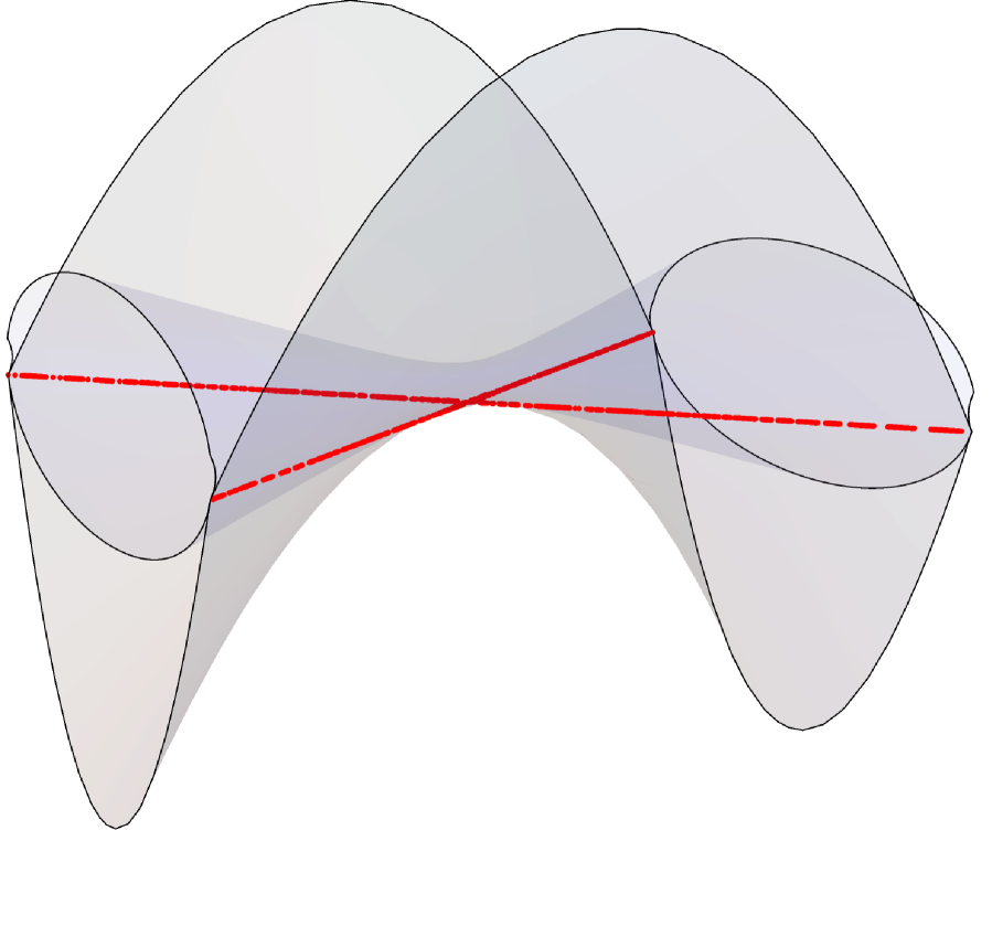
(b)

Figure 5: (a) Base set of the surface type $D_{5}^{(1)}$: four pairs of infinitely near points on two double generators. (b) Pencil of quadrics tangent along a pair of intersecting lines.

The vertical switch $i_{1}$ and the horizontal switch $i_{2}$ for this pencil are given by the following formulas:

$$i_{1}(x,y)=(x,\widetilde{y}),\quad{\rm where}\quad\widetilde{y}+y=b_{1}+b_{3}+\frac{a_{6}}{x-a_{5}}+\frac{a_{8}}{x-a_{7}},$$ (130)

$$i_{2}(x,y)=(\widetilde{x},y),\quad{\rm where}\quad\widetilde{x}+x=a_{5}+a_{7}+\frac{b_{2}}{y-b_{1}}+\frac{b_{4}}{y-b_{3}}.$$ (131)

The maps $i_{1}$, $i_{2}$ have four “long” singularity confinement patterns:

$$\{y=b_{1}\}\;\;\stackrel{{\scriptstyle i_{2}}}{{\to}}\;\>s_{2}\;\;\stackrel{{\scriptstyle i_{1}}}{{\to}}\;\>s_{4}\;\;\stackrel{{\scriptstyle i_{2}}}{{\to}}\;\;\{y=b_{3}\},$$ (132)

$$\{y=b_{3}\}\;\;\stackrel{{\scriptstyle i_{2}}}{{\to}}\;\>s_{4}\;\;\stackrel{{\scriptstyle i_{1}}}{{\to}}\;\>s_{2}\;\;\stackrel{{\scriptstyle i_{2}}}{{\to}}\;\;\{y=b_{1}\},$$ (133)

$$\{x=a_{5}\}\;\;\stackrel{{\scriptstyle i_{1}}}{{\to}}\;\>s_{6}\;\;\stackrel{{\scriptstyle i_{2}}}{{\to}}\;\>s_{8}\;\;\stackrel{{\scriptstyle i_{1}}}{{\to}}\;\;\{x=a_{7}\},$$ (134)

$$\{x=a_{7}\}\;\;\stackrel{{\scriptstyle i_{1}}}{{\to}}\;\>s_{8}\;\;\stackrel{{\scriptstyle i_{2}}}{{\to}}\;\>s_{6}\;\;\stackrel{{\scriptstyle i_{1}}}{{\to}}\;\;\{x=a_{5}\}.$$ (135)

We give here the “naive” singularity confinement patterns. This means that we display blow-down of $\mathcal{C}(i_{1})$, $\mathcal{C}(i_{2})$ under $i_{1}$, resp. $i_{2}$; thus, we do not perform the “last” blow-ups which regularize the lifts of these maps.

Lifting to 3D.

We now lift this to a 3D QRT map. The curve $C_{\infty}$ is lifted to the quadric $P_{\infty}=\{X_{4}^{2}=0\}$, and we consider the pencil of quadrics

$$Q_{\lambda}=\big{\{}X_{1}X_{2}-X_{3}X_{4}-\lambda X_{4}^{2}=0\big{\}}.$$ (136)

The base set of the pencil $Q_{\lambda}$ consists of two double lines $\{X_{1}=X_{4}=0\}$ and $\{X_{2}=X_{4}=0\}$, see Fig. 5 (b). The intersection of this base set with the base set of the pencil $\{P_{\mu}\}$ consists of eight points

$$S_{1}=[1:0:b_{1}:0],\;\;S_{3}=[1:0:b_{3}:0],\;\;S_{5}=[0:1:a_{5}:0],\;\;S_{7}=[0:1:a_{7}:0],$$

$$S_{2}=[1:b_{1}\epsilon:b_{1}+b_{2}\epsilon:\epsilon],\;\;S_{4}=[1:b_{3}\epsilon:b_{3}+b_{4}\epsilon:\epsilon],$$

$$S_{6}=[a_{5}\epsilon:1:a_{5}+a_{6}\epsilon:\epsilon],\;\;S_{8}=[a_{7}\epsilon:1:a_{7}+a_{8}\epsilon:\epsilon],$$ (137)

where $S_{2},S_{4},S_{6},S_{8}$ are understood as infinitely near points to $S_{1},S_{3},S_{5},S_{7}$, respectively.

Transforming $Q_{\lambda}$ to the canonical form.

The characteristic polynomial of the pencil $\{Q_{\lambda}\}$ is: $\Delta(\lambda)=\det(M_{\lambda})=1$, so that ${\rm Sing}(Q)=\{\infty\}$. The normalizing transformation of $Q_{\lambda}$ to the canonical form $Q_{0}$ is:

$$\begin{bmatrix}X_{1}\\ X_{2}\\ X_{3}\\ X_{4}\end{bmatrix}=\begin{bmatrix}Y_{1}\\ Y_{2}\\ Y_{3}-\lambda Y_{4}\\ Y_{4}\end{bmatrix}=A_{\lambda}\begin{bmatrix}Y_{1}\\ Y_{2}\\ Y_{3}\\ Y_{4}\end{bmatrix},\quad A_{\lambda}=\begin{pmatrix}1&0&0&0\\ 0&1&0&0\\ 0&0&1&-\lambda\\ 0&0&0&1\end{pmatrix}.$$ (138)

This gives the following parametrization of $Q_{\lambda}$:

$$\begin{bmatrix}X_{1}\\ X_{2}\\ X_{3}\\ X_{4}\end{bmatrix}=A_{\lambda}\begin{bmatrix}x\\ y\\ xy\\ 1\end{bmatrix}=\begin{bmatrix}x\\ y\\ xy-\lambda\\ 1\end{bmatrix}=:\phi_{\lambda}(x,y).$$ (139)

The pencil-adapted coordinates $(x,y,\lambda)$ on ${\mathbb{P}}^{3}$ are:

$$x=\frac{X_{1}}{X_{4}}=\frac{X_{3}+\lambda X_{4}}{X_{2}},\quad y=\frac{X_{2}}{X_{4}}=\frac{X_{3}+\lambda X_{4}}{X_{1}},\quad\lambda=\frac{X_{1}X_{2}-X_{3}X_{4}}{X_{4}^{2}}.$$ (140)

Computing the 3D QRT map.

Proposition 8

In the pencil-adapted coordinates $(x,y,\lambda)$, for each fixed $\lambda$, the intersection curves $Q_{\lambda}\cap P_{\mu}$ form the pencil $\phi_{\lambda}^{*}P_{\mu}$ which can be characterized as the pencil of biquadratic curves in ${\mathbb{P}}^{1}\times{\mathbb{P}}^{1}$ through the eight points

$$s_{1}(\lambda)=(\infty,b_{1}),\quad s_{3}(\lambda)=(\infty,b_{3}),\quad s_{5}(\lambda)=(a_{5},\infty),\quad s_{7}(\lambda)=(a_{7},\infty),$$

$$s_{2}(\lambda)=(\epsilon^{-1},b_{1}+(b_{2}+\lambda)\epsilon),\quad s_{4}(\lambda)=(\epsilon^{-1},b_{3}+(b_{4}+\lambda)\epsilon),$$

$$s_{6}(\lambda)=(a_{5}+(a_{6}+\lambda)\epsilon,\epsilon^{-1}),\quad s_{8}(\lambda)=(a_{7}+(a_{8}+\lambda)\epsilon,\epsilon^{-1}).$$ (141)

The latter points correspond to $S_{1},\ldots,S_{8}$ given in (12) under the map $\phi_{\lambda}^{-1}$. The curve $C_{\infty}(\lambda)$ coincides with $C_{\infty}$. Formulas for the involutions $i_{1}$, $i_{2}$ restricted to $Q_{\lambda}$ are obtained from (130), (131) by replacing $b_{i}\mapsto b_{i}+\lambda$ for $i=2,4$, and $a_{i}\mapsto a_{i}+\lambda$ for $i=6,8$:

$$i_{1}|_{Q_{\lambda}}(x,y)=(x,\widetilde{y}),\quad{\rm where}\quad\widetilde{y}+y=b_{1}+b_{3}+\frac{a_{6}+\lambda}{x-a_{5}}+\frac{a_{8}+\lambda}{x-a_{7}},$$ (142)

$$i_{2}|_{Q_{\lambda}}(x,y)=(\widetilde{x},y),\quad{\rm where}\quad\widetilde{x}+x=a_{5}+a_{7}+\frac{b_{2}+\lambda}{y-b_{1}}+\frac{b_{4}+\lambda}{y-b_{3}}.$$ (143)

The maps $i_{1}|_{Q_{\lambda}}$, $i_{2}|_{Q_{\lambda}}$ admit four “long” singularity confinement patterns of the type (132)–(135). These can be reformulated as (25) for $(i,j)=$  (2,4), (4,2), and as (26) for $(i,j)=$  (6,8), (8,6), if we set

$$\Psi_{2}=\{X_{2}-b_{1}X_{4}=0\}, \Psi_{4}=\{X_{2}-b_{3}X_{4}=0\},$$

$$\Phi_{6}=\{X_{1}-a_{5}X_{4}=0\}, \Phi_{8}=\{X_{1}-a_{7}X_{4}=0\}.$$

The birational involutions $i_{1},i_{2}$ of $\mathbb{P}^{3}$ are of $\deg=3$. For instance, $i_{1}:[X_{1}:X_{2}:X_{3}:X_{4}]\mapsto[\widetilde{X}_{1}:\widetilde{X}_{2}:\widetilde{X}_{3}:\widetilde{X}_{4}]$, where

$$\widetilde{X}_{1} = X_{1}(X_{1}-a_{5}X_{4})(X_{1}-a_{7}X_{4}),$$

$$\widetilde{X}_{2} = X_{1}^{2}X_{2}-2X_{1}X_{3}X_{4}+(b_{1}+b_{3})X_{1}^{2}X_{4}+(a_{5}+a_{7})X_{3}X_{4}^{2}-a_{5}a_{7}X_{2}X_{4}^{2}$$

$$+\big{(}a_{6}+a_{8}-(b_{1}+b_{3})(a_{5}+a_{7})\big{)}X_{1}X_{4}^{2}-\big{(}a_{6}a_{7}+a_{5}a_{8}-a_{5}a_{5}(b_{1}+b_{3})\big{)}X_{4}^{3},$$

$$\widetilde{X}_{3} = -X_{1}^{2}X_{3}+(b_{1}+b_{3})X_{1}^{3}+(a_{5}+a_{7})X_{1}^{2}X_{2}+a_{5}a_{7}X_{3}X_{4}^{2}-2a_{5}a_{7}X_{1}X_{2}X_{4}$$

$$+\big{(}a_{6}+a_{8}-(b_{1}+b_{3})(a_{5}+a_{7})\big{)}X_{1}^{2}X_{4}-\big{(}a_{6}a_{7}+a_{5}a_{8}-a_{5}a_{5}(b_{1}+b_{3})\big{)}X_{1}X_{4}^{2},$$

$$\widetilde{X}_{4} = X_{4}(X_{1}-a_{5}X_{4})(X_{1}-a_{7}X_{4}).$$

Deforming a 3D QRT map to a discrete Painlevé equation.

Since in the present case ${\rm Sing}(Q)=\{\infty\}$, we can take $\sigma(\lambda)=\lambda+\delta$, and since the equation for the base curve $C_{\infty}(\lambda)$ is the same on every $Q_{\lambda}$, we can set $L|_{Q_{\lambda}}=A_{\lambda+\delta}A_{\lambda}^{-1}$ as the deformation map. We easily compute that $L|_{Q_{\lambda}}$ only depends on $\delta$ but not on $\lambda$:

$$L:\quad[X_{1}:X_{2}:X_{3}:X_{4}]\to[X_{1}:X_{2}:X_{3}-\delta X_{4}:X_{4}].$$ (144)

Theorem 5

Consider the pencil of quadrics (136), the corresponding birational involutions $i_{1},i_{2}$, and the linear map (144). Define the birational maps $\widetilde{i}_{1}=L\circ i_{1}$, $\widetilde{i}_{2}=L\circ i_{2}$, and $\widetilde{f}=\widetilde{i}_{1}\circ\widetilde{i}_{2}$. Then $\widetilde{f}$ sends each quadric $Q_{\lambda}$ to $Q_{\lambda+2\delta}$ and has the following singularity confinement patterns:

• (34)  for $(i,j)=(2,4),(4,2)$,

• (37)  for $(i,j)=(6,8),(8,6)$.

If one parametrizes $Q_{\lambda}$ by $(x,y)\in{\mathbb{P}}^{1}\times{\mathbb{P}}^{1}$ according to (116), then in coordinates $(x,y,\lambda)$ on ${\mathbb{P}}^{3}$ the map $\widetilde{f}:(x_{n},y_{n},\lambda_{2n})\mapsto(x_{n+1},y_{n+1},\lambda_{2n+2})$ is equivalent to the additive Painlevé equation of the type $D_{5}^{(1)}$, a system of two non-autonomous difference equations:

$$x_{n+1}+x_{n} = a_{5}+a_{7}+\frac{b_{2}+\lambda_{2n}}{y_{n}-b_{1}}+\frac{b_{4}+\lambda_{2n}}{y_{n}-b_{3}},$$ (145)

$$y_{n+1}+y_{n} = b_{1}+b_{3}+\frac{a_{6}+\lambda_{2n+1}}{x_{n+1}-a_{5}}+\frac{a_{8}+\lambda_{2n+1}}{x_{n+1}-a_{7}},$$ (146)

where $\lambda_{n}=n\delta+\lambda_{0}$.

Proof. Follows from Proposition 3 by observing that:

• The map $L$ fixes the points $S_{1},S_{3},S_{5},S_{7}$, while it maps the infinitely near points as follows:

  $$L(S_{2})=[1:b_{1}\epsilon:b_{1}+(b_{2}-\delta)\epsilon:\epsilon],\quad L(S_{4})=[1:b_{3}\epsilon:b_{3}+(b_{4}-\delta)\epsilon:\epsilon],$$

  $$L(S_{6})=[a_{5}\epsilon:1:a_{5}+(a_{6}-\delta)\epsilon:\epsilon],\quad L(S_{8})=[a_{7}\epsilon:1:a_{7}+(a_{8}-\delta)\epsilon:\epsilon];$$

• $L\circ i_{1}$ maps $L(S_{2})$ to $S_{4}$ and $L(S_{4})$ to $S_{2}$;

• $L\circ i_{2}$ maps $L(S_{6})$ to $S_{8}$ and $L(S_{8})$ to $S_{6}$.

This is easily shown by a fiber-wise computation. We notice also that $L$ fixes the four planes $\Psi_{2}$, $\Psi_{4}$, $\Phi_{6}$, $\Phi_{6}$. $\blacksquare$

Remark. The eight points participating in the singularity confinement patterns for $\widetilde{f}$ are: the four points $S_{1},S_{3},S_{5},S_{7}$ and the four infinitely near points $S_{2},S_{4},L(S_{6}),L(S_{8})$. If $\delta\neq 0$, they support a one-dimensional linear system of quadrics, namely the pencil $Q_{\lambda}$. If $\delta=0$, this set becomes the two-dimensional net spanned by $\{Q_{\lambda}\}$ and $\{P_{\mu}\}$.

13 Additive discrete Painlevé equation of the type $A_{1}^{(1)}$ from a pencil of the type (viii)

We consider here a pencil of quadrics in ${\mathbb{P}}^{3}$ with the base curve being the union of a twisted cubic and a tangent line to it. Such pencil can be taken as

$$Q_{\lambda}=\big{\{}X_{1}X_{2}-X_{3}X_{4}-\lambda(X_{1}^{2}-X_{2}X_{4})=0\big{\}}.$$ (147)

The base curve is:

$$\big{\{}[t:t^{2}:t^{3}:1]:t\in{\mathbb{P}}^{1}\big{\}}\cup\{X_{1}=X_{4}=0\}.$$ (148)

On the quadric $Q_{0}$, with the standard parametrization $[X_{1}:X_{2}:X_{3}:X_{4}]=[x:y:xy:1]$, the base curve becomes a biquadratic curve on ${\mathbb{P}}^{1}\times{\mathbb{P}}^{1}$ with equation $\{x^{2}-y=0\}$. It has two irreducible components:

$$C_{\infty}:\quad\{y=x^{2}\}\cup\{y=\infty\},$$ (149)

a (2,1)-curve and a horizontal generator.

(a)

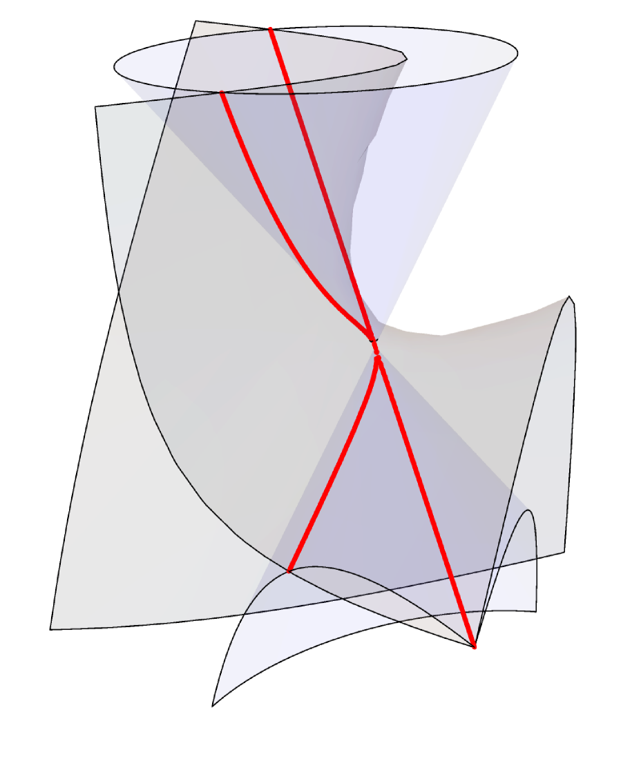
(b)

Figure 6: (a) Base set of the surface type $A_{1}^{(1)}$: six points on a (2,1)-curve and two points on a generator tangent to it. (b) Pencil of quadrics through a twisted cubic and one of its tangent lines.

2D QRT map.

We construct a QRT map with base points lying on the biquadratic curve (149). One easily checks that eight points

$$s_{i}=(a_{i},a_{i}^{2}),\;i=1,\ldots,6,\quad s_{7}=(a_{7},\infty),\quad s_{8}=(a_{8},\infty)$$ (150)

support a pencil of biquadraric curves $C_{\mu}$ (including the curve $C_{\infty}$) if and only if the following condition is satisfied:

$$a_{1}+a_{2}+a_{3}+a_{4}+a_{5}+a_{6}=a_{7}+a_{8}.$$ (151)

We define $i_{1}$ and $i_{2}$ as the vertical and the horizontal switches with respect to this pencil, and we define the QRT map $f=i_{1}\circ i_{2}$. The formulas for the involutions $i_{1}$ and $i_{2}$ can be written compactly in terms of the following equations:

$$i_{1}(x,y)=(x,\widetilde{y}),\quad(\widetilde{y}-x^{2})(y-x^{2})=\frac{\prod_{i=1}^{6}(x-a_{i})}{(x-a_{7})(x-a_{8})},$$ (152)

$$i_{2}(x,y)=(\widetilde{x},y),\quad\frac{(\widetilde{x}-\eta)(x-\eta)}{(\widetilde{x}+\eta)(x+\eta)}=\frac{\prod_{i=1}^{6}(\eta-a_{i})}{\prod_{i=1}^{6}(\eta+a_{i})},\quad y=\eta^{2}.$$ (153)

The last equation has to be understood as follows: equation (153) is invariant under $\eta\to-\eta$ and therefore only depends on $\eta^{2}$ (when put in the polynomial form). Thus, it defines $\widetilde{x}$ as a rational function of $x$ and $y=\eta^{2}$. Birational involutions $i_{1}$, $i_{2}$ on ${\mathbb{P}}^{1}\times{\mathbb{P}}^{1}$ admit six “short” singularity confinement patterns (5) and two “long” singularity confinement patterns of the type (9).

Lifting to 3D.

We lift the pencil of biquadratric curves $C_{\mu}$ to a pencil of quadrics $P_{\mu}$ in ${\mathbb{P}}^{3}$. Then we consider the pencil $Q_{\lambda}$ given in (147), spanned by $Q_{0}$ and $P_{\infty}$. The base set of the pencil $Q_{\lambda}$ consists, as already mentioned, of a twisted cubic and its tangent line, as given in (148). The intersection of this base set with the base set of the pencil $\{P_{\mu}\}$ consists of eight points

$$S_{i}=[a_{i}:a_{i}^{2}:a_{i}^{3}:1],\;i=1,\ldots,6,\quad S_{7}=[0:1:a_{7}:0],\quad S_{8}=[0:1:a_{8}:0].$$ (154)

Transforming $Q_{\lambda}$ to the canonical form.

The characteristic polynomial of the pencil $\{Q_{\lambda}\}$ is: $\Delta(\lambda)=\det(M_{\lambda})=1$, so that ${\rm Sing}(Q)=\{\infty\}$. The normalizing transformation of $Q_{\lambda}$ to the canonical form $Q_{0}$ is:

$$\begin{bmatrix}X_{1}\\ X_{2}\\ X_{3}\\ X_{4}\end{bmatrix}=\begin{bmatrix}Y_{1}\\ Y_{2}+\lambda Y_{1}\\ Y_{3}+\lambda Y_{2}+\lambda^{2}Y_{3}\\ Y_{4}\end{bmatrix}=A_{\lambda}\begin{bmatrix}Y_{1}\\ Y_{2}\\ Y_{3}\\ Y_{4}\end{bmatrix},\quad A_{\lambda}=\begin{pmatrix}1&0&0&0\\ \lambda&1&0&0\\ \lambda^{2}&\lambda&1&0\\ 0&0&0&1\end{pmatrix}.$$ (155)

This immediately gives the following parametrization of $Q_{\lambda}$:

$$\left[\begin{array}[]{c}X_{1}\\ X_{2}\\ X_{3}\\ X_{4}\end{array}\right]=\left[\begin{array}[]{c}x\\ y+\lambda x\\ xy+\lambda y+\lambda^{2}x\\ 1\end{array}\right]=:\phi_{\lambda}(x,y).$$ (156)

The pencil-adapted coordinates $(x,y,\lambda)$ on ${\mathbb{P}}^{3}$ are:

$$x=\frac{X_{1}}{X_{4}}=\frac{X_{3}-\lambda X_{2}}{X_{2}-\lambda X_{1}},\quad y=\frac{X_{2}-\lambda X_{1}}{X_{4}}=\frac{X_{3}-\lambda X_{2}}{X_{1}},\quad\lambda=\frac{X_{1}X_{2}-X_{3}X_{4}}{X_{1}^{2}-X_{2}X_{4}}.$$ (157)

Computing the 3D QRT map.

Proposition 9

In the pencil-adapted coordinates $(x,y,\lambda)$, for each fixed $\lambda$, the intersection curves $Q_{\lambda}\cap P_{\mu}$ form the pencil $\phi_{\lambda}^{*}P_{\mu}$ which can be characterized as the pencil of biquadratic curves in ${\mathbb{P}}^{1}\times{\mathbb{P}}^{1}$ through the eight points

$$s_{i}(\lambda)=(a_{i},a_{i}^{2}-\lambda a_{i}),\;i=1,\ldots,6,\quad s_{7}(\lambda)=(a_{7}-\lambda,\infty),\quad s_{8}(\lambda)=(a_{8}-\lambda,\infty),$$ (158)

which correspond to $S_{1},\ldots,S_{8}$ given in (154) under the map $\phi_{\lambda}^{-1}$. The curve $C_{\infty}(\lambda)$ is given by

$$C_{\infty}(\lambda):\quad\{y=x^{2}-\lambda x\}\cup\{y=\infty\}.$$ (159)

The formulas for the involutions $i_{1}$, $i_{2}$ restricted to $Q_{\lambda}$:

$$i_{1}|_{Q_{\lambda}}(x,y)=(x,\widetilde{y}),\quad\big{(}\widetilde{y}-x(x-\lambda)\big{)}\big{(}y-x(x-\lambda)\big{)}=\frac{\prod_{i=1}^{6}(x-a_{i})}{(x-a_{7}+\lambda)(x-a_{8}+\lambda)},$$ (160)

$$i_{2}|_{Q_{\lambda}}(x,y)=(\widetilde{x},y),\quad\frac{(\widetilde{x}-\eta)(x-\eta)}{(\widetilde{x}+\eta-\lambda)(x+\eta-\lambda)}=\frac{\prod_{i=1}^{6}(\eta-a_{i})}{\prod_{i=1}^{6}(\eta+a_{i}-\lambda)},\quad y=\eta(\eta-\lambda).$$ (161)

Formulas for the birational involutions $i_{1}$, $i_{2}$ in homogeneous coordinates $X$ on ${\mathbb{P}}^{3}$ can be obtained by conjugating (160), (161) by $\phi$. We omit the resulting formulas.

The maps $i_{1}|_{Q_{\lambda}}$, $i_{2}|_{Q_{\lambda}}$ admit six “short” singularity confinement patterns of the types (21) and two “long” singularity confinement patterns of the type (23). They are easily translated to homogeneous coordinates, becoming (24) for $i=1,\ldots,6$, and (26) for $(i,j)=$(7,8) and (8,7). One computes with the help of (157) the equations of the surfaces $\Psi_{i}$ and $\Phi_{i}$:

$$\Phi_{i}=\{X_{1}-a_{i}X_{4}=0\},\quad i=1,\ldots,6,$$ (162)

$$\Psi_{i}=\{X_{1}X_{3}-X_{2}^{2}-a_{i}^{2}(X_{1}^{2}-X_{2}X_{4})+a_{i}(X_{1}X_{2}-X_{3}X_{4})=0\},\quad i=1,\ldots,6,$$ (163)

$$\Phi_{i}=\{X_{1}^{3}-X_{3}X_{4}^{2}-a_{i}X_{4}(X_{1}^{2}-X_{2}X_{4})=0\},\quad i=7,8.$$ (164)

Deforming a 3D QRT map to a discrete Painlevé equation.

In the present case ${\rm Sing}(Q)=\{\infty\}$, so that we can take $\sigma(\lambda)=\lambda+\delta$. The fiberwise construction (27) requires to find $\psi_{\lambda}:{\mathbb{P}}^{1}\times{\mathbb{P}}^{1}\to{\mathbb{P}}^{1}\times{\mathbb{P}}^{1}$ which maps the curve $C_{\infty}(\lambda)$ to $C_{\infty}(\lambda+\delta)$. In the present example, we should have $\psi_{\lambda}(x,y)=(\hat{x},\hat{y})$ such that

$$\hat{y}=\infty\;\Leftrightarrow\;y=\infty,\quad\hat{y}=\hat{x}^{2}-(\lambda+\delta)\hat{x}\;\Leftrightarrow\;y=x^{2}-\lambda x.$$

The solution with $\hat{x}=x$ is given by

$$\psi_{\lambda}:\quad\hat{x}=x,\quad\hat{y}=y-\delta x.$$ (165)

Now a direct computation with (27) and (156) results in

$$L:\begin{bmatrix}X_{1}\\ X_{2}\\ X_{3}\\ x_{4}\end{bmatrix}\;\mapsto\;\begin{bmatrix}\hat{X}_{1}\\ \hat{X}_{2}\\ \hat{X}_{3}\\ \hat{X}_{4}\end{bmatrix}=\begin{bmatrix}X_{1}X_{4}\\ X_{2}X_{4}\\ X_{3}X_{4}+\delta(X_{2}X_{4}-X_{1}^{2})\\ X_{4}^{2}\end{bmatrix}.$$ (166)

Unlike in all the previous examples, where the deformation map $L$ was a projective linear map in ${\mathbb{P}}^{3}$, here it is a birational map of degree 2. Its critical set is $\mathcal{C}(L)=\{X_{4}=0\}$, while its indeterminacy set is $\mathcal{I}(L)=\{X_{1}=X_{4}=0\}$.

Note that the twisted cubic $\{[t:t^{2}:t^{3}:1]:\,t\in{\mathbb{P}}^{1}\}$ is fixed by the deformation map $L$. In particular, the same is true for the base points $S_{i}$, $i=1,\ldots,6$. On the other hand, $S_{7},S_{8}\in\mathcal{I}(L)$. In the next Theorem 6, we will nevertheless use the points which we denote (by abuse of notation)

$$L(S_{7})=[0:1:a_{7}+\delta:0],\quad L(S_{8})=[0:1:a_{8}+\delta:0].$$ (167)

Let us comment on this. Actually, our considerations in Theorem 6 are fiber-wise, i.e., on individual quadrics $Q_{\lambda}$. This gives us effectively a blow-up of the set $\mathcal{I}(L)$, which is described in the pencil-adapted coordinates as $\{y=\infty\}$, so that the point with homogeneous coordinates $[0:1:a:0]\in\mathcal{I}(L)$ has coordinates $(a-\lambda,\infty)$ on $Q_{\lambda}$. In pencil-adapted coordinates $(x,y,\lambda)$ the action of $L$ is described by

$$L:(x,y,\lambda)\mapsto(x,y-\delta x,\lambda+\delta),$$ (168)

Thus, as long as $\lambda\neq\infty$, any point $(a-\lambda,\infty)\in Q_{\lambda}$ is mapped to $(a-\lambda,\infty)\in Q_{\lambda+\delta}$ with homogeneous coordinates $[0:1:a+\delta:0]$. For $a=a_{7},a_{8}$, this justifies formulas (167) away from $Q_{\infty}$.

Theorem 6

Consider the pencil of quadrics (147), the corresponding birational involutions $i_{1}$, $i_{2}$, and the birational deformation map (166). Define the birational maps $\widetilde{i}_{1}=L\circ i_{1}$, $\widetilde{i}_{2}=L\circ i_{2}$, and $\widetilde{f}=\widetilde{i}_{1}\circ\widetilde{i}_{2}$. Then $\widetilde{f}$ sends each quadric $Q_{\lambda}$ to $Q_{\lambda+2\delta}$ and, away from $Q_{\infty}$, it has the following singularity confinement patterns:

• (31)  for $1,\ldots,6$,

• (37)  for $(i,j)=(7,8),(8,7)$.

If one parametrizes $Q_{\lambda}$ by $(x,y)\in{\mathbb{P}}^{1}\times{\mathbb{P}}^{1}$ according to (156), then in coordinates $(x,y,\lambda)$ on ${\mathbb{P}}^{3}$ the map $\widetilde{f}:(x_{n},y_{n},\lambda_{2n})\mapsto(x_{n+1},y_{n+1},\lambda_{2n+2})$ is equivalent to an additive Painlevé equation of the type $A_{1}^{(1)}$, the system of two non-autonomous difference equations:

$$\frac{(x_{n+1}-\eta_{n})(x_{n}-\eta_{n})}{(x_{n+1}+\eta_{n}-\lambda_{2n})(x_{n}+\eta_{n}-\lambda_{2n})}=\frac{\prod_{i=1}^{6}(\eta_{n}-a_{i})}{\prod_{i=1}^{6}(\eta_{n}+a_{i}-\lambda_{2n})},\quad y_{n}=\eta_{n}(\eta_{n}-\lambda_{2n}),$$ (169)

$$\big{(}y_{n+1}-x_{n+1}(x_{n+1}-\lambda_{2n+2})\big{)}\big{(}y_{n}-x_{n+1}(x_{n+1}-\lambda_{2n})\big{)}$$ (170)

$$\qquad\qquad=\frac{\prod_{i=1}^{6}(x_{n+1}-a_{i})}{(x_{n+1}-a_{7}+\lambda_{2n+1})(x_{n+1}-a_{8}+\lambda_{2n+1})},$$

where $\lambda_{n}=\delta n+\lambda_{0}$.

Proof. The patterns (31) involving $S_{i}$, $i=1,\ldots,6$ follow from Proposition 3 by observing that these points are fixed by the deformation map $L$. For the patterns (37) involving the points $L(S_{7})$, $L(S_{8})$, we make the fiberwise computation. On the quadric $Q_{\lambda}$, $i_{2}$ maps $(x,\infty)$ to $(a_{7}+a_{8}-2\lambda-x,\infty)$. Therefore, we have

$$\{x=a_{7}-\lambda\}\;{\rm on}\;Q_{\lambda}$$

$$\quad\xrightarrow[]{i_{1}}(a_{7}-\lambda,\infty)\;{\rm on}\;Q_{\lambda}\xrightarrow[]{L}(a_{7}-\lambda,\infty)\;{\rm on}\;Q_{\lambda+\delta}$$

$$\quad\xrightarrow[]{i_{2}}(a_{8}-(\lambda+2\delta),\infty)\;{\rm on}\;Q_{\lambda+\delta}\xrightarrow[]{L}(a_{8}-(\lambda+2\delta),\infty)\;{\rm on}\;Q_{\lambda+2\delta}$$

$$\quad\xrightarrow[]{i_{1}}\{x=a_{8}-(\lambda+2\delta)\}\;{\rm on}\;Q_{\lambda+2\delta}\xrightarrow[]{L}\{x=a_{8}-(\lambda+2\delta)\}\;{\rm on}\;Q_{\lambda+3\delta}.$$

This can be written (away from $Q_{\infty}$) as

$$\Phi_{7}\xrightarrow[]{\widetilde{i}_{1}}L(S_{7})\xrightarrow[]{\widetilde{i}_{2}}S_{8}\xrightarrow[]{\widetilde{i}_{1}}L(\Phi_{8}).$$ (171)

In terms of $\widetilde{f}=\widetilde{i}_{1}\circ\widetilde{i}_{2}$, this gives (37), as usual. As for the equations of motion, (169) is obtained from (161) by $\lambda\leftarrow\lambda_{2n}$, $x\leftarrow x_{n}$, $\widetilde{x}\leftarrow x_{n+1}$, and $\eta\leftarrow\eta_{n}$. Similarly, (170) is obtained from (160) by $\lambda\leftarrow\lambda_{2n+1}$, $x\leftarrow x_{n+1}$, $y\leftarrow y_{n}-\delta x_{n+1}$, and $\widetilde{y}\leftarrow y_{n+1}+\delta x_{n+1}$. $\blacksquare$

Remark. As pointed out in the introduction, the discrete Painlevé equations of this and the next sections seem to be different from those encountered in the literature. In particular, equations related to the surface type $A_{1}^{(1)}$ given in [13] come from a different realization of such surfaces. Sakai uses in [20] the same realization as ours (up to a canonical birational isomorphism between $\mathbb{P}^{2}$ and $\mathbb{P}^{1}\times\mathbb{P}^{1}$), but he does not give the corresponding discrete Painlevé equations explicitly.

14 Multiplicative discrete Painlevé equation of the type $A_{1}^{(1)}$ from a pencil of the type (vii)

As the last example, we consider a pencil of quadrics in $\mathbb{P}^{3}$ with the base curve being the union of a twisted cubic and its secant (i.e., a line intersecting the twisted cubic at two points). Such pencil can be taken as

$$Q_{\lambda}=\big{\{}X_{1}X_{2}-X_{3}X_{4}-\lambda Q_{\infty}(X)=0\big{\}},$$ (172)

where

$$Q_{\infty}(X)=X_{1}^{2}-X_{2}X_{4}+b^{2}(X_{2}^{2}-X_{1}X_{3}).$$ (173)

Here $b$ is a free parameter. We recover the case considered in the previous section in the limit $b\to 0$. The base curve is:

$$\big{\{}[t:t^{2}:t^{3}:1]:t\in{\mathbb{P}}^{1}\big{\}}\cup\{X_{1}-b^{2}X_{3}=X_{4}-b^{2}X_{2}=0\}.$$ (174)

On the quadric $Q_{0}$, with the standard parametrization $[X_{1}:X_{2}:X_{3}:X_{4}]=[x:y:xy:1]$, the equation of the base curve reads $\{(x^{2}-y)(1-b^{2}y)=0\}$. It has two irreducible components:

$$C_{\infty}:\quad\{y=x^{2}\}\cup\{y=1/b^{2}\},$$ (175)

a (2,1)-curve and a horizontal line. See Fig. 7 (a).

(a)

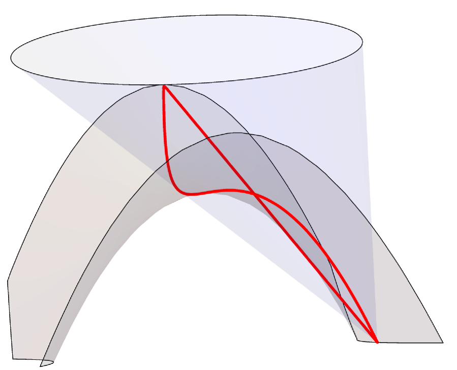
(b)

Figure 7: (a) Base set of the surface type $A_{1}^{(1)}$: six points on a (2,1)-curve and two points on a secant horizontal generator. (b) Pencil of quadrics through a twisted cubic and one of its secant lines.

2D QRT map.

Consider the following eight points lying on the biquadratic curve (175):

$$s_{i}=(a_{i},a_{i}^{2}),\;i=1,\ldots,6,\quad s_{7}=(a_{7},1/b^{2}),\quad s_{8}=(a_{8},1/b^{2}).$$ (176)

They support a pencil of biquadraric curves $C_{\mu}$ (including the curve $C_{\infty}$) if and only if the following condition is satisfied:

$$\prod_{i=1}^{6}\frac{(1+ba_{i})}{(1-ba_{i})}=\frac{(1+ba_{7})(1+ba_{8})}{(1-ba_{7})(1-ba_{8})}.$$ (177)

The vertical and the horizontal switches with respect to this pencil are given by:

$$i_{1}(x,y)=(x,\widetilde{y}),\quad\frac{(\widetilde{y}-x^{2})(y-x^{2})}{(1-b^{2}\widetilde{y})(1-b^{2}y)}=A\frac{\prod_{i=1}^{6}(x-a_{i})}{(x-a_{7})(x-a_{8})},$$ (178)

where

$$A=\frac{(1+ba_{7})(1+ba_{8})}{\prod_{i=1}^{6}(1+ba_{i})},$$ (179)

and

$$i_{2}(x,y)=(\widetilde{x},y),\quad\frac{(\widetilde{x}-\eta)(x-\eta)}{(\widetilde{x}+\eta)(x+\eta)}=\frac{\prod_{i=1}^{6}(\eta-a_{i})}{\prod_{i=1}^{6}(\eta+a_{i})},\quad y=\eta^{2}.$$ (180)

Lifting to 3D.

We lift the pencil of biquadratric curves $C_{\mu}$ to a pencil of quadrics $P_{\mu}$ in ${\mathbb{P}}^{3}$. Then we consider the pencil $Q_{\lambda}$ given in (172), spanned by $Q_{0}$ and $P_{\infty}$. The base set of the pencil $Q_{\lambda}$ consists, as already mentioned, of a twisted cubic and its tangent line, as given in (174). The intersection of this base set with the base set of the pencil $\{P_{\mu}\}$ consists of eight points

$$S_{i}=[a_{i}:a_{i}^{2}:a_{i}^{3}:1],\;i=1,\ldots,6,\quad S_{7}=[b^{2}a_{7}:1:a_{7}:b^{2}],\quad S_{8}=[b^{2}a_{8}:1:a_{8}:b^{2}].$$ (181)

Transforming $Q_{\lambda}$ to the canonical form.

The characteristic polynomial of the pencil $\{Q_{\lambda}\}$ is easily computed: $\Delta(\lambda)=\det(M_{\lambda})=(1-b^{2}\lambda^{2})^{2}$, so that ${\rm Sing}(Q)=\{1/b,-1/b\}$. The normalizing transformation of $Q_{\lambda}$ to the canonical form $Q_{0}$ is:

$$\begin{bmatrix}Y_{1}\\ Y_{2}\\ Y_{3}\\ Y_{4}\end{bmatrix}=\begin{bmatrix}X_{1}-b^{2}\lambda X_{2}\\ X_{2}-\lambda X_{1}\\ X_{3}-\lambda X_{2}\\ X_{4}-b^{2}\lambda X_{1}\end{bmatrix}=A_{\lambda}^{-1}\begin{bmatrix}X_{1}\\ X_{2}\\ X_{3}\\ X_{4}\end{bmatrix},\quad A_{\lambda}^{-1}=\begin{pmatrix}1&-b^{2}\lambda&0&0\\ -\lambda&1&0&0\\ 0&-\lambda&1&0\\ -b^{2}\lambda&0&0&1\end{pmatrix}.$$ (182)

This gives the following parametrization of $Q_{\lambda}$:

$$\begin{bmatrix}X_{1}\\ X_{2}\\ X_{3}\\ X_{4}\end{bmatrix}=A_{\lambda}\begin{bmatrix}x\\ y\\ xy\\ 1\end{bmatrix}=\begin{bmatrix}x+b^{2}\lambda y\\ \lambda x+y\\ \lambda^{2}x+\lambda y+(1-b^{2}\lambda^{2})xy\\ b^{2}\lambda x+b^{4}\lambda^{2}y+(1-b^{2}\lambda^{2})\end{bmatrix}=:\phi_{\lambda}(x,y).$$ (183)

The pencil-adapted coordinates $(x,y,\lambda)$ on ${\mathbb{P}}^{3}$ are:

$$x=\frac{X_{1}-b^{2}\lambda X_{2}}{X_{4}-b^{2}\lambda X_{1}}=\frac{X_{3}-\lambda X_{2}}{X_{2}-\lambda X_{1}},\qquad y=\frac{X_{2}-\lambda X_{1}}{X_{4}-b^{2}\lambda X_{1}}=\frac{X_{3}-\lambda X_{2}}{X_{1}-b^{2}\lambda X_{2}},$$ (184)

$$\lambda=\frac{X_{1}X_{2}-X_{3}X_{4}}{X_{1}^{2}-X_{2}X_{4}+b^{2}(X_{2}^{2}-X_{1}X_{3})}.$$ (185)

Computing the 3D QRT map.

Proposition 10

In the pencil-adapted coordinates $(x,y,\lambda)$, for each fixed $\lambda$, the intersection curves $Q_{\lambda}\cap P_{\mu}$ form the pencil $\phi_{\lambda}^{*}P_{\mu}$ which can be characterized as the pencil of biquadratic curves in ${\mathbb{P}}^{1}\times{\mathbb{P}}^{1}$ through the eight points

$$s_{i}(\lambda)=\big{(}a_{i},a_{i}\sigma(a_{i},\lambda)\big{)},\;i=1,\ldots,6,\quad$$ (186)

$$s_{7}(\lambda)=\big{(}\sigma(a_{7},\lambda),1/b^{2}\big{)},\quad s_{8}(\lambda)=\big{(}\sigma(a_{8},\lambda),1/b^{2}\big{)},$$ (187)

which correspond to $S_{1},\ldots,S_{8}$ given in (181) under the map $\phi_{\lambda}^{-1}$. Here we use the abbreviation $\sigma(a,\lambda)=(a-\lambda)/(1-b^{2}\lambda a)$. The curve $C_{\infty}(\lambda)$ is given by

$$C_{\infty}(\lambda):\quad\{y=x\sigma(x,\lambda)\}\cup\{y=1/b^{2}\}.$$ (188)

For the involutions $i_{1}$, $i_{2}$ we have: $i_{1}|_{Q_{\lambda}}(x,y)=(x,\widetilde{y})$, resp. $i_{2}|_{Q_{\lambda}}(x,y)=(\widetilde{x},y)$, where $\widetilde{y}$, resp. $\widetilde{x}$ satisfy the equations

$$(1-b^{2}\lambda x)^{2}\frac{\big{(}\widetilde{y}-x\sigma(x,\lambda)\big{)}\big{(}y-x\sigma(x,\lambda)\big{)}}{(1-b^{2}\widetilde{y})(1-b^{2}y)}=\frac{A(1-b^{2}\lambda^{2})^{2}}{(1-b^{2}\lambda a_{7})(1-b^{2}\lambda a_{8})}\frac{\prod_{i=1}^{6}(x-a_{i})}{\big{(}x-\sigma(a_{7},\lambda)\big{)}\big{(}x-\sigma(a_{8},\lambda)\big{)}},$$ (189)

$$\frac{1}{(1-b^{2}\lambda\eta)^{2}}\frac{(\widetilde{x}-\eta)(x-\eta)}{\big{(}\widetilde{x}+\sigma(\eta,\lambda)\big{)}\big{(}x+\sigma(\eta,\lambda)\big{)}}=\frac{(1-b^{2}\lambda^{2})^{2}}{\prod_{i=1}^{6}(1-b^{2}\lambda a_{i})}\frac{\prod_{i=1}^{6}(\eta-a_{i})}{\prod_{i=1}^{6}\big{(}\eta+\sigma(a_{i},\lambda)\big{)}},\quad y=\eta\sigma(\eta,\lambda).$$ (190)

Formulas for the birational involutions $i_{1}$, $i_{2}$ in homogeneous coordinates $X$ on ${\mathbb{P}}^{3}$ can be obtained by conjugating (189), (190) by $\phi$. We omit the resulting formulas.

The maps $i_{1}|_{Q_{\lambda}}$, $i_{2}|_{Q_{\lambda}}$ admit six “short” singularity confinement patterns of the types (21) and two “long” singularity confinement patterns of the type (23). They are easily translated to homogeneous coordinates, becoming (24) for $i=1,\ldots,6$, and (26) for $(i,j)=$(7,8) and (8,7). One computes with the help of (184) the equations of the surfaces $\Psi_{i}$ and $\Phi_{i}$:

$$\Phi_{i}= \{X_{1}-b^{2}X_{3}-a_{i}(X_{4}-b^{2}X_{2})=0\},\quad i=1,\ldots,6,$$ (191)

$$\Psi_{i}= \{X_{1}X_{3}-X_{2}^{2}-a_{i}^{2}(X_{1}^{2}-X_{2}X_{4})+a_{i}(X_{1}X_{2}-X_{3}X_{4})=0\},\quad i=1,\ldots,6,$$ (192)

$$\Phi_{i}= \{X_{1}^{3}-X_{3}X_{4}^{2}-a_{i}X_{4}(X_{1}^{2}-X_{2}X_{4})-2b^{2}X_{3}(X_{1}^{2}-X_{2}X_{4})-b^{4}X_{3}(X_{2}^{2}-X_{1}X_{3})$$

$$-2b^{2}a_{i}X_{4}(X_{2}^{2}-X_{1}X_{3})+b^{4}a_{i}(X_{2}^{3}-X_{3}^{2}X_{4})=0\},\quad i=7,8.$$ (193)

Deforming a 3D QRT map to a discrete Painlevé equation.

We have ${\rm Sing}(Q)=\{\ 1/b,$ $-1/b\}$, so an automorphism of $\mathbb{P}^{1}$ fixing the points of ${\rm Sing}(Q)$ can be taken as

$$\sigma(\lambda)=\frac{\lambda+\delta}{1+b^{2}\delta\lambda}.$$

The fiberwise construction (27) requires to find $\psi_{\lambda}:{\mathbb{P}}^{1}\times{\mathbb{P}}^{1}\to{\mathbb{P}}^{1}\times{\mathbb{P}}^{1}$ which maps the curve $C_{\infty}(\lambda)$ to $C_{\infty}(\sigma(\lambda))$. In the present example, we should have $\psi_{\lambda}(x,y)=(\hat{x},\hat{y})$ such that

$$\hat{y}=\frac{1}{b^{2}}\;\Leftrightarrow\;y=\frac{1}{b^{2}},\quad\hat{y}(1-b^{2}\hat{\lambda}\hat{x})-\hat{x}(\hat{x}-\hat{\lambda})=0\;\Leftrightarrow\;y(1-b^{2}\lambda x)-x(x-\lambda)=0,$$

where $\hat{\lambda}=\sigma(\lambda)$. The solution with $\hat{x}=x$ is easily computed:

$$\psi_{\lambda}:\quad\hat{x}=x,\quad\hat{y}=y-\frac{\delta x(1-b^{2}\lambda^{2})(1-b^{2}y)}{1+b^{2}\delta\lambda-b^{2}(\lambda+\delta)x}.$$ (194)

A direct computation with (27) and (183) results in a pretty complicated birational map $L$ on $\mathbb{P}^{3}$ of degree 4. Its indeterminacy set $\mathcal{I}(L)$ coincides with the base curve (174) of the pencil $\{Q_{\lambda}\}$ and consists of the twisted cubic and its secant line. Like in the case of Section 13, the fibration of $\mathbb{P}^{3}$ by the quadrics $Q_{\lambda}$ gives us effectively a blow-up of $\mathcal{I}(L)$. Straightforward computations show that, away from the two degenerate quadrics $Q_{\pm 1/b}$, the map $L$ fixes the twisted cubic pointwise, and acts on the line $\{X_{1}-b^{2}X_{3}=X_{4}-b^{2}X_{2}=0\}$ according to the formula

$$L([b^{2}a:1:a:b^{2}])=[b^{2}(a+\delta):1+\delta b^{2}a:a+\delta:b^{2}(1+\delta b^{2}a)].$$

Indeed, $L$ maps the point with pencil-adapted coordinates $(x,y)=(\sigma(a,\lambda),1/b^{2})\in Q_{\lambda}$ to the point with the pencil-adapted coordinates $(x,y)=(\sigma(a,\lambda),1/b^{2})\in Q_{\sigma(\lambda)}$, which computes with the help of (183) in homogeneous coordinates to the above expression. Thus, on all $Q_{\lambda}$ with $\lambda\notin{\rm Sing}(Q)$, the images $\psi_{\lambda}(s_{i}(\lambda))$ are well defined and are given in homogeneous coordinates on $\mathbb{P}^{3}$ by $L(S_{i})=S_{i}$, $i=1,\ldots,6$, and

$$L(S_{7}) = [b^{2}(a_{7}+\delta):1+\delta b^{2}a_{7}:a_{7}+\delta:b^{2}(1+\delta b^{2}a_{7})],$$

$$L(S_{8}) = [b^{2}(a_{8}+\delta):1+\delta b^{2}a_{8}:a_{8}+\delta:b^{2}(1+\delta b^{2}a_{8})].$$

Now we give a theorem whose formulation and proof are completely analogous to Theorem 6.

Theorem 7

Consider the pencil of quadrics (172), the corresponding birational involutions $i_{1}$, $i_{2}$, and the birational deformation map $L$ described above. Define the birational maps $\widetilde{i}_{1}=L\circ i_{1}$, $\widetilde{i}_{2}=L\circ i_{2}$, and $\widetilde{f}=\widetilde{i}_{1}\circ\widetilde{i}_{2}$. Then $\widetilde{f}$ sends each quadric $Q_{\lambda}$ to $Q_{\sigma^{2}(\lambda)}$ and, away from $Q_{\pm 1/b}$, it has the following singularity confinement patterns:

• (31)  for $1,\ldots,6$,

• (37)  for $(i,j)=(7,8),(8,7)$.

If one parametrizes $Q_{\lambda}$ by $(x,y)\in{\mathbb{P}}^{1}\times{\mathbb{P}}^{1}$ according to (183), then in coordinates $(x,y,\lambda)$ on ${\mathbb{P}}^{3}$ the map $\widetilde{f}:(x_{n},y_{n},\lambda_{2n})\mapsto(x_{n+1},y_{n+1},\lambda_{2n+2})$, with $\lambda_{n}=\sigma^{n}(\lambda_{0})$, is equivalent to a multiplicative Painlevé equation of the type $A_{1}^{(1)}$. The latter is the system of two non-autonomous difference equations, the first one being obtained from (190) by $\lambda\leftarrow\lambda_{2n}$, $x\leftarrow x_{n}$, $\widetilde{x}\leftarrow x_{n+1}$, and $\eta\leftarrow\eta_{n}$, and the second one being obtained from (189) by $\lambda\leftarrow\lambda_{2n+1}$,

$$(x,y)\leftarrow\psi_{\lambda_{2n+1}}(x_{n+1},y_{n}),\quad and\quad(x,\widetilde{y})\leftarrow\psi_{\lambda_{2n+2}}^{-1}(x_{n+1},y_{n+1}).$$

15 Conclusions

After having elaborated in detail on the novel geometric scheme including a large portion of discrete Painlevé equations, several directions for further investigations can be sketched.

1. For the seven classes of pencils of quadrics considered above, our present construction consists in a Painlevé modification of 3D QRT maps, which are defined using involutions along generators of the pencil. However, these are not the only interesting geometric involutions in this context. In [17], further classes of Manin involutions were defined for pencils of higher-degree planar curves of genus 1. These novel Manin involutions can be also generalized to dimension 3. For instance, a 3D generalization of the Manin involution $I_{ij}^{(2)}$ for a pencil of quartic curves with two double points can be proposed as follows. Consider two pencils of quadrics $\{Q_{\lambda}\}$ and $\{P_{\mu}\}$ sharing one common quadric $P_{\infty}$, and let $S_{i}$, $i=1,\ldots,8$ be the base set of the net of quadrics spanned by these two pencils. Fix two indices $i,j\in\{1,\ldots,8\}$. For a generic $X\in{\mathbb{P}}^{3}$ (not belonging to the base set of either pencil), determine $\lambda,\mu\in{\mathbb{P}}^{1}$ such that $X\in Q_{\lambda}\cap P_{\mu}$; define $I_{i,j}(X)$ to be the fourth intersection point of the curve $Q_{\lambda}\cap P_{\mu}$ with the plane through $S_{i}$, $S_{j}$, and $X$. Compositions of such involutions $I_{i,j}$ provide us with novel integrable maps on $\mathbb{P}^{3}$ preserving the quadrics of both pencils. Their Painlevé deformations are definitely worth a detailed study.

2. The most urgent problem is to develop a more general scheme capable of the treatment of the six pencils left open in the present paper. One of the main problems to overcome here is the non-rationality (over $\mathbb{P}^{3}$) of the corresponding 3D QRT maps. This will be addressed in the forthcoming paper [2].

3. It can be anticipated that our scheme provides a natural framework for the isomonodromic description of discrete Painlevé equations. This will also be the subject of our ongoing research.

4. It would be important to work out the relation of our present approach to the previous study of integrable birational maps on $\mathbb{P}^{3}$ related to configurations of eight points [21].

References

- [1] J. Alonso, Yu. B. Suris, K. Wei. A three-dimensional generalization of QRT maps. J. Nonlinear Sci. 33 (2023), article Nr. 117, 27 pp.
- [2] J. Alonso, Yu. B. Suris, K. Wei. Discrete Painlevé equations and nets of quadrics (in preparation).
- [3] M. P. Bellon, C.-M. Viallet. Algebraic entropy. Commun. Math. Phys. 204 (1999), 425–437.
- [4] A.S. Carstea, A. Dzhamay, T. Takenawa. Fiber-dependent deautonomization of integrable 2D mappings and discrete Painlevé equations. J. Phys. A. Math. Theor. 50 (2017), 405202 (41 pp).
- [5] E. Casas-Alvero. Analytic projective geometry. EMS Textbooks in Mathematics. Zürich: European Mathematical Society (2014), xvi+620 pp.
- [6] J. Diller. Dynamics of birational maps of . Indiana Univ. Math. J., 45 (1996), 721–772.
- [7] J. Diller, C. Favre. Dynamics of bimeromorphic maps of surfaces. Amer. J. Math. 123 (2001), 1135–1169.
- [8] J.J. Duistermaat. Discrete Integrable Systems. QRT Maps and Elliptic Surfaces. Springer Monographs in Mathematics. Springer, New York (2010), xxii+627 pp.
- [9] B. Grammaticos, A. Ramani. Discrete Painlevé equations: a review. In: Grammaticos, B. et al. (eds.), Discrete integrable systems, Proceedings of the international CIMPA school, Pondicherry, India, February 2–14, 2003. Lecture Notes in Physics 644 (2004), 245–321.
- [10] B. Grammaticos, A. Ramani, V. Papageorgiou. Do integrable mappings have the Painlevé property? Phys. Rev. Lett. 67, No. 14 (1991) 1825–1828.
- [11] H. P. Hudson. Cremona transformations in plane and space, Cambridge University Press, 1927.
- [12] N. Joshi. Discrete Painlevé equations. CBMS Regional Conference Series in Mathematics 131. Providence, RI: American Mathematical Society (2019), vi+146 pp.
- [13] K. Kajiwara, M. Noumi, Y. Yamada. Geometric aspects of Painlevé equations. J. Phys. A. Math. Theor. 50 (2017), 073001 (164 pp).
- [14] T. Mase, R. Willox, A. Ramani, and B. Grammaticos. Singularity confinement as an integrability criterion, J. Phys. A 52 (2019), 205201, 29 pp.
- [15] G.R.W. Quispel, J.A.G. Roberts, C.J.Thompson. Integrable mappings and soliton equations. Phys. Lett. A 126, no. 7 (1988) 419–421.
- [16] G.R.W. Quispel, J.A.G. Roberts, C.J.Thompson. Integrable mappings and soliton equations II. Phys. D 34, no. 1–2 (1989) 183–192.
- [17] M. Petrera, Yu.B. Suris, Kangning Wei, R. Zander. Manin involutions for elliptic pencils and discrete integrable systems. Math. Phys. Anal. Geom., 24:6 (2021), 26 pp.
- [18] A. Ramani, B. Grammaticos, J. Hietarinta. Discrete versions of the Painlevé equations. Phys. Rev. Lett. 67, No. 14 (1991) 1829–1832.
- [19] M. Reid. The complete intersection of two or more quadrics. Thesis, Cambridge, 1972. http://homepages.warwick.ac.uk/masda/3folds/qu.pdf
- [20] H. Sakai. Rational surfaces associated with affine root systems and geometry of the Painlevé equations. Commun. Math. Phys. 220 (2001), 165–229.
- [21] T. Takenawa. Discrete dynamical systems associated with the configuration space of 8 points in . Commun. Math. Phys. 246, No. 1 (2004) 19–42 .