Robustness of the data-driven approach in limited angle tomography

Abstract.

The limited angle Radon transform is notoriously difficult to invert due to the ill-posedness. In this work, we give a mathematical explanation that the data-driven approach based on deep neural networks can reconstruct more information in a stable way compared to traditional methods.

1. Introduction

Consider the limited angle Radon transform on ${\mathbb{R}}^{2}$. Let $(x_{1},x_{2})$ be the coordinate for ${\mathbb{R}}^{2}$. For $\delta\in(0,\pi/2),$ let ${\mathcal{S}}_{\delta}=\{(\cos\theta,\sin\theta)\in{\mathbb{S}}^{1}:|\theta|\leq\delta\}.$ We use the parallel beam parametrization of the Radon transform. Let $v\in{\mathcal{S}}_{\delta}$ and $v^{\perp}$ be the unit vector orthogonal to $v$ so that $\{v,v^{\perp}\}$ has the same orientation as the coordinate frame. The limited angle Radon transform of a function $f$ on ${\mathbb{R}}^{2}$ is

(1) $$R_{\delta}f(p,v)=\int_{{\mathbb{R}}}\chi_{\delta}(v)f(pv+tv^{\perp})dt,\quad v\in{\mathbb{S}}^{1},p\in{\mathbb{R}}$$

where $\chi_{\delta}$ is the characteristic function of ${\mathcal{S}}_{\delta}$ in ${\mathbb{S}}^{1}.$ For simplicity, we assume that $f$ is supported in the unit disk ${\mathcal{B}}=\{x\in{\mathbb{R}}^{2}:|x|<1\}$ where $|\cdot|$ stands for the Euclidean norm. It is a classical result that $R_{\delta}$ is injective on compactly supported distributions, see for instance [9, 14]. However, the inverse problem of recovering $f$ from $R_{\delta}f$ is severely ill-posed. This was demonstrated from the behavior of the singular values in [4]. On the microlocal level, it’s clear that some information of $f$ is lost. In particular, Quinto in [10] gave a microlocal description of the singularities of $f$ that can be recovered, called “visible singularities”, and those that cannot, called “invisible singularities”, see Section 2. Due to the ill-posedness, traditional methods such as filtered back-projection or iterative methods often produce artifacts in the reconstruction, and it is very challenging to recover the invisible information.

Recently, there are increasing efforts in applying the data-driven approach such as deep neural networks to the limited angle tomography, see for example [1, 2, 3, 6, 7, 12] and references therein. Multiple numerical experiments reported that the data-driven approach can significantly reduce the artifact phenomena and even learn the invisible singularities. The success seems difficult to understand from the existing mathematical theory. Also, the robustness of the data-driven approach is a concern, see for example [8]. It is suspected that the data-driven approach should be tailored to specific tasks, not for general image reconstruction. But a precise understanding is still missing.

The goal of this paper is to provide a mathematical explanation. It is useful to interpret the instability of the limited angle Radon transform from the following view point: there is no stability estimate of the form

(2) $$\|f\|_{H^{s}({\mathbb{R}}^{2})}\leq C(s,t)\|R_{\delta}f\|_{H^{s+t}({\mathbb{R}}\times{\mathbb{S}}^{1})}$$

for any $s,t\in{\mathbb{R}}$, see Section VI.2 of [9]. This is because, roughly speaking, after taking the limited angle Radon transform, the Fourier transform $\hat{f}$ of $f$ is lost in a conic region (corresponding to the missing angles), see Figure 1. Recovery of $\hat{f}$ in the rest of the Fourier space (${\mathcal{K}}_{\delta}$ in Figure 1) however is stable, see Theorem 3.1. This result is sharp. For the data-driven approach, we consider $f$ in a training data set ${\mathcal{D}}$ and show that $\hat{f}$ can be stably recovered in a larger cone (${\mathcal{K}}_{\delta+\epsilon}$ in Figure 1), see Theorem 3.2. The size of the cone depends on ${\mathcal{D}}$ and it is possible to cover the whole Fourier space for certain ${\mathcal{D}}$. This explains the phenomena of “learning the invisible”. We remark that our theory does not rely on the specific structure of the neural network. In Section 4, we use a simple U-net to test our theory. The concluding summary is offered in Section 5.

Figure 1. Illustration of the increased stability in the Fourier space. Traditional methods can recover $\hat{f}$ in the cone ${\mathcal{K}}_{\delta}$ (defined in Section 3). The data-driven approach can recover $\hat{f}$ in a larger cone ${\mathcal{K}}_{\delta+\epsilon}$. The size of the cone depends on the specific training set.

2. The visible and invisible singularities

In [11], Quinto described some principles on recovering features of an object from limited X-ray CT. Roughly speaking, if a boundary of a feature of the body is tangent to a line in a limited data set, then that boundary should be easy to reconstruct (called visible boundaries). Otherwise, the boundary should be difficult to reconstruct from the limited data (called invisible boundaries). We use the filtered backprojection reconstruction to demonstrate the principle.

Let $\theta\in(-\delta,\delta)$ and define the limited angle back-projection for $R_{\delta}$ as

$$R^{*}_{\delta}g(x)=\int_{-\delta}^{\delta}g(v(\theta),x\cdot v(\theta))d\theta.$$

Let $\Lambda$ be the Riesz potential

$$\Lambda g(v,p)=\frac{1}{2\pi}\int_{-\infty}^{\infty}\int_{-\infty}^{\infty}e^{i\tau(p-s)}|\tau|g(v,s)dsd\tau.$$

Then we consider the following FBP for limited angle transform

(3) $$L_{\delta}f=\frac{1}{4\pi}R_{\delta}^{*}\Lambda R_{\delta}f.$$

Note that this is not an inversion formula. We describe what can be reconstructed from this formula.

We introduce some notions from microlocal analysis. Let $f$ be a function on ${\mathbb{R}}^{2}$ and let $x_{0}\in{\mathbb{R}}^{2},\xi_{0}\in{\mathbb{R}}^{2}\backslash 0$. By definition, $f$ is smooth at $x_{0}$ in direction $\xi_{0}$ if there is a smooth function $\phi\in C_{c}^{\infty}({\mathbb{R}}^{2})$ with $\phi(x_{0})\neq 0$ and an open cone ${\mathscr{V}}$ containing $\xi_{0}$ such that for any $N\in{\mathbb{N}}$ there is $C_{N}$ such that

$$|\widehat{\phi f}(\xi)|\leq C_{N}(1+|\xi|)^{-N},\text{for all }\xi\in{\mathscr{V}}.$$

where $\hat{}$ denotes the Fourier transform in ${\mathbb{R}}^{2}.$ If $f$ is not smooth at $x_{0}$ in direction $\xi_{0}$, then $(x_{0},\xi_{0})\in\text{WF}(f)$ the wavefront set of $f$. Let $(x_{0},\xi_{0})\in\text{WF}(f).$ We say $(x_{0},\xi_{0})$ is a visible singularity of $f$ (for $L_{\delta}$) if $\xi_{0}$ is parallel to some $v\in{\mathcal{S}}_{\delta}$. We say $(x_{0},\xi_{0})$ is an invisible singularity of $f$ if $\xi_{0}$ is not parallel for any $v\in{\mathcal{S}}_{\delta}$. We have

Theorem 2.1 (Theorem 2 of [11]).

Let $f$ be a function of compact support and $(x_{0},\xi_{0})\in\text{WF}(f)$.

1. If $(x_{0},\xi_{0})$ is a visible singularity of $f$ then $(x_{0},\xi_{0})\in\text{WF}(L_{\delta}f)$.

2. If $(x_{0},\xi_{0})$ is an invisible singularity of $f$ then $(x_{0},\xi_{0})\notin\text{WF}(L_{\delta}f)$.

We remark that it is possible to obtain the more precise microlocal Sobolev regularity of the visible singularities, see Theorem 3.1 of [11]. Within the microlocal framework, one can also explain the artifact phenomena. For our setup, the artifact can occur on lines parallel to $v\in\partial{\mathcal{S}}_{\delta}$ and the lines are tangent to the boundary of some feature in the object, see Principle 2 of [10].

3. The stable reconstruction

We establish quantitative estimate for recovering visible singularities. Our starting point is the simple injectivity proof for $R_{\delta}$, see [9, Theorem 3.4]. The transform $R_{\delta}f(p,v)$ is a function defined on ${\mathbb{R}}\times{\mathbb{S}}^{1}.$ We take Fourier transform of $R_{\delta}f$ in $p$ to get

(4) $$\widehat{R_{\delta}f}(\tau,v) =\int_{\mathbb{R}}\int_{\mathbb{R}}e^{-\imath p\tau}\chi_{\delta}(v)f(pv+tv^{\perp})dtdp$$

$$=\int_{\mathbb{R}}\int_{\mathbb{R}}e^{-\imath(pv+tv^{\perp})\cdot\tau v}\chi_{\delta}(v)f(pv+tv^{\perp})dtdp=\hat{f}(\tau v)\chi_{\delta}(v).$$

Here, $\imath^{2}=-1$. Because $R_{\delta}f(p,v)=0$, we get $\hat{f}(\xi)=0$ for $\xi\in{\mathbb{R}}^{2}$ parallel to $v$. Thus $\hat{f}(\xi)=0$ in a cone ${\mathcal{K}}_{\delta}=\{\xi\in{\mathbb{R}}^{2}:\xi/|\xi|\in{\mathcal{S}}_{\delta}\}$ with non-empty interior for $\delta>0$. Because $\hat{f}$ is analytic in $\xi$, we conclude that $\hat{f}(\xi)=0$ for all $\xi\in{\mathbb{R}}^{2}.$ So $f=0$ after taking the inverse Fourier transform.

We can further derive some stability estimate. Below we also use $\chi_{\delta}$ for the characteristic function of ${\mathcal{K}}_{\delta}$ in ${\mathbb{R}}^{2}.$ It should be clear from the context which one we are referring to.

Theorem 3.1.

For $\delta\in(0,\pi/2]$ and $f\in H^{-1/2}({\mathbb{R}}^{2}),$ we have

(5) $$\|\chi_{\delta}(D)f\|_{H^{-1/2}({\mathbb{R}}^{2})}\leq\|R_{\delta}f\|_{L^{2}({\mathbb{R}}\times{\mathbb{S}}^{1})}.$$

Proof.

Applying Plancherel’s theorem and using (4), we get

(6) $$\|R_{\delta}f\|^{2}_{L^{2}({\mathbb{R}}\times{\mathbb{S}}^{1})}= \|\widehat{R_{\delta}f}\|^{2}_{L^{2}({\mathbb{R}}\times{\mathbb{S}}^{1})}=\int_{{\mathbb{S}}^{1}}\int_{{\mathbb{R}}}\chi_{\delta}(v)|\hat{f}(\tau v)|^{2}d\tau dv$$

$$= \int_{{\mathcal{K}}_{\delta}}|\xi|^{-1}|\hat{f}(\xi)|^{2}d\xi\geq\|\chi_{\delta}(D)f\|_{H^{-1/2}({\mathbb{R}}^{2})}^{2}.$$

This finishes the proof. ∎

The theorem essentially is a quantitative version of Theorem 2.1 on stably recovering visible singularities of $f$. It is also clear that the stability estimate (2) fails because of $(1-\chi_{\delta}(D))f$ which sits in the kernel of $R_{\delta}.$

We seek improvement of the estimate to include invisible singularities. For $\epsilon>0$ small we define $\chi_{\delta+\epsilon}(D)$ as a Fourier multiplier of $\chi_{\delta+\epsilon}(\xi),\xi\in{\mathbb{R}}^{2}$. For $N\geq 0$, we define

(7) $$\begin{gathered}{\mathcal{D}}_{N,\epsilon}=\{f\in L^{2}({\mathcal{B}}):\|f\|_{L^{2}}\leq N\|\chi_{\delta+\epsilon}(D)f\|_{H^{-1/2}}\}.\end{gathered}$$

Observe that $L^{2}({\mathcal{B}})=\cup_{N\geq 0}{\mathcal{D}}_{N,\epsilon}.$ The following theorem says that for functions in ${\mathcal{D}}_{N,\epsilon}$, the stability estimate (5) can be improved.

Theorem 3.2.

For $N\geq 0$, there is $\epsilon>0$ small such that

(8) $$\|\chi_{\delta+\epsilon}(D)f\|_{H^{-1/2}({\mathbb{R}}^{2})}\leq 2\|R_{\delta}f\|_{L^{2}({\mathbb{R}}\times{\mathbb{S}}^{1})}$$

for all $f\in{\mathcal{D}}_{N,\epsilon}.$

Proof.

We decompose

(9) $$R_{\delta}f=R_{\delta}\chi_{\delta+\epsilon}(D)f+R_{\delta}(1-\chi_{\delta+\epsilon}(D))f.$$

Note that the second term on the right vanishes because $(1-\chi_{\delta+\epsilon}(D))f$ is in the kernel of $R_{\delta}.$ So we estimate the first term. Using (4), we have

(10) $$R_{\delta}\chi_{\delta+\epsilon}(D)f(p,v)-R_{\delta+\epsilon}\chi_{\delta+\epsilon}(D)f(p,v)$$

$$= (2\pi)^{-1}\int_{\mathbb{R}}e^{\imath p\tau}(\chi_{\delta}(v)-\chi_{\delta+\epsilon}(v))\chi_{\delta+\epsilon}(\tau v)\hat{f}(\tau v)d\tau.$$

Note that $\chi_{\delta}(v)-\chi_{\delta+\epsilon}(v)$ is supported in a set of ${\mathbb{S}}^{1}$ with measure $<C\epsilon.$ Also, the left hand side of (10) is compactly supported in $p$. Using Plancherel’s theorem again, we get

(11) $$\|R_{\delta}\chi_{\delta+\epsilon}(D)f-R_{\delta+\epsilon}\chi_{\delta+\epsilon}(D)f\|_{L^{2}}^{2}$$

$$\leq C\int_{{\mathbb{R}}}\int_{{\mathbb{S}}^{1}}|(\chi_{\delta}(v)-\chi_{\delta+\epsilon}(v))\chi_{\delta+\epsilon}(\tau v)\hat{f}(\tau v)|^{2}dvd\tau$$

$$\leq C\epsilon^{2}\left(\int_{{\mathbb{R}}}\int_{{\mathbb{S}}^{1}}|\chi_{\delta+\epsilon}(\tau v)\hat{f}(\tau v)|^{4}d\tau dv\right)^{\frac{1}{2}}$$

$$\leq C\epsilon^{2}\pi\|f\|_{L^{2}}\left(\int_{{\mathbb{R}}}\int_{{\mathbb{S}}^{1}}|\hat{f}(\tau v)|^{2}d\tau dv\right)^{\frac{1}{2}}$$

$$\leq C\epsilon^{2}\pi\sqrt{4\pi^{2}+1}\|f\|_{L^{2}}^{2}\leq 20C\epsilon^{2}N^{2}\|\chi_{\delta+\epsilon}(D)f\|^{2}_{H^{-1/2}}.$$

where $C$ is an absolute constant independent of $\epsilon,N,f$. Also in the derivation, we used Hölder’s inequality and the fact that $\|\hat{h}\|_{L^{\infty}}\leq\sqrt{\pi}\|h\|_{L^{2}}$ for $h$ compactly supported in $\mathcal{B}$ and

$$\int_{{\mathbb{R}}}\int_{{\mathbb{S}}^{1}}|\hat{f}(\tau v)|^{2}d\tau dv =\int_{|\tau|\geq 1}\int_{{\mathbb{S}}^{1}}|\hat{f}(\tau v)|^{2}d\tau dv+\int_{|\tau|<1}\int_{{\mathbb{S}}^{1}}|\hat{f}(\tau v)|^{2}d\tau dv$$

$$\leq\int_{|\tau|\geq 1}\int_{{\mathbb{S}}^{1}}|\tau||\hat{f}(\tau v)|^{2}d\tau dv+\pi\|f\|_{L^{2}}^{2}\int_{|\tau|<1}\int_{{\mathbb{S}}^{1}}1d\tau dv$$

$$\leq(1+4\pi^{2})\|f\|_{L^{2}}^{2}.$$

We can apply Theorem 3.1 to derive that

$$\|\chi_{\delta+\epsilon}(D)f\|_{H^{-1/2}} \leq\|R_{\delta+\epsilon}\chi_{\delta+\epsilon}(D)f\|_{L^{2}}$$

$$\leq\|R_{\delta}\chi_{\delta+\epsilon}(D)f\|_{L^{2}}+\|R_{\delta}\chi_{\delta+\epsilon}(D)f-R_{\delta+\epsilon}\chi_{\delta+\epsilon}(D)f\|_{L^{2}}$$

$$\leq\|R_{\delta}\chi_{\delta+\epsilon}(D)f\|_{L^{2}}+\sqrt{20C}\epsilon N\|\chi_{\delta+\epsilon}(D)f\|_{H^{-1/2}}.$$

For $\epsilon>0$ sufficiently small so that $\sqrt{20C}\epsilon N<1/2$, we obtain

(12) $$\|\chi_{\delta+\epsilon}(D)f\|_{H^{-1/2}({\mathbb{R}}^{2})}\leq 2\|R_{\delta}\chi_{\delta+\epsilon}(D)f\|_{L^{2}({\mathbb{R}}\times{\mathbb{S}}^{1})},$$

which finishes the proof. ∎

We remark that we chose the Sobolev norms in the condition in (7) for simplicity. The analysis can be adapted to other Sobolev functions by slightly modifying the proof of Theorem 3.1 and 3.2. For neural networks, suppose the training is done on a finite data set ${\mathcal{D}}\subset H^{-1/2}$. Then one can always find $N>0$ and $\epsilon>0$ so that ${\mathcal{D}}\subset{\mathcal{D}}_{N,\epsilon}$. Suppose the neural network algorithm is capable of learning an integral operator (e.g. universal approximation property is achieved). Then the learned inversion operator $R^{-1}_{\delta}$ would potentially satisfy the improved stability estimate (8) which can explain the stable reconstruction of some invisible singularities.

4. The experiment

4.1. The neural network

We use the same data as in [3] which can be downloaded from [15]. The data set consists of synthetic images of ellipses, where the number, locations, sizes and the intensity gradients of the ellipses are chosen at random. The measurements are computed using the Matlab function radon with added Gaussian noise. Also, the measurements are simulated at a higher resolution and then downsampled to an image of resolution $128\times 128$ to avoid the inverse crime. For the simulation below, we use measurements for a missing wedge of $80^{\circ}$ (out of $180^{\circ}$). See Figure 3.

For the network structure, we first use Matlab function iradon to compute the FBP inversion. Then we use a basic U-net [13] with network structure plotted in Figure 2. We use $500$ images for training the network among which $80\%$ are used for training and $20\%$ for validation. We show two examples of the reconstruction on test images in Figure 4. We observe that in both examples artifacts are almost completely removed, and some of the invisible singularities are also constructed well. But we do notice that the reconstructions are not perfect. Several thin ellipses with mainly invisible singularities are not reconstructed at all in both examples.

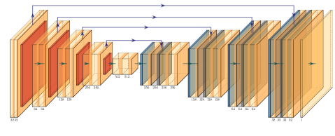
Figure 2. Structure of the U-net. The input is a $128\times 128$ image and the output is also a $128\times 128$ image. The number of channels is indicated in the boxes. The arrows indicate the flow of the data.

4.2. The robustness

We consider violation of the condition in (7). For $a>0$, we consider the characteristic function for the disk centered at $0$ with radius $a$

$$f_{a}(x)=1\text{ for }|x|<a\text{ and }f_{a}(x)=0\text{ for }|x|\geq a.$$

Taking Fourier transform in ${\mathbb{R}}^{2}$ and using polar coordinate, we get

$$\begin{gathered}\hat{f}_{a}(\xi)=\int_{{\mathbb{S}}^{1}}\int_{0}^{a}e^{-ir\omega\cdot\xi}rdrd\omega=\int_{{\mathbb{S}}^{1}}\int_{0}^{1}e^{-ir\omega\cdot a\xi}a^{2}rdrd\omega=a^{2}\hat{f}_{1}(a\xi).\end{gathered}$$

Below, we use homogeneous Sobolev spaces to compute

$$\begin{gathered}\|\chi_{\delta+\epsilon}(D)f_{a}\|_{\dot{H}^{-1/2}}^{2}=\int_{{\mathbb{R}}^{2}}|\xi|^{-1}\chi_{\delta+\epsilon}(\xi)^{2}|\hat{f}_{a}(\xi)|^{2}d\xi\\ =\int_{{\mathbb{R}}^{2}}|\xi|^{-1}\chi_{\delta+\epsilon}(\xi)^{2}a^{4}|\hat{f}_{1}(a\xi)|^{2}d\xi=\int_{{\mathbb{R}}^{2}}|\xi/a|^{-1}\chi_{\delta+\epsilon}(\xi/a)^{2}a^{2}|\hat{f}_{1}(\xi)|^{2}d\xi.\end{gathered}$$

We see that for $a$ large,

$$\|\chi_{\delta+\epsilon}(D)f_{a}\|_{\dot{H}^{-1/2}}\simeq a^{3/2}\|\chi_{\delta+\epsilon}(D)f_{1}\|_{\dot{H}^{-1/2}}.$$

Similarly, we have $\|f_{a}\|_{L^{2}}\simeq a\|f_{1}\|_{L^{2}}$. If $\|f_{1}\|_{L^{2}}$ $\leq C_{0}\|\chi_{\delta+\epsilon}(D)f_{1}\|_{H^{-1/2}}$ is true for some $C_{0}>0$, then for $f_{a}$, the condition in (7) will be violated when $a$ is large. We show the test result for this example in Figure 5. As $a$ increases, we start to see instabilities in the network reconstruction and eventually artifacts start to appear, which agrees with our theory.

We also test the trained network on other types of images, see the two squares in Figure 6. We know that the corners could produce strong artifacts as shown in the FBP reconstruction. Because the two squares are not too large, condition (7) is likely to be satisfied via similar Fourier analysis as for $f_{a}$. The numerical result agrees with our observation.

4.3. Further discussions

The examples presented in Sections 4.1 and 4.2 indicate that the trained neural network is a good approximation of $R_{\delta}^{-1}$. However, we do not claim that every trained network shares the same property. In fact, we tested training the network for a longer time and observed that the training error may still decrease, but the test results on general images in Section 4.2 usually become worse. This might be a sign of overfitting. The discussion of the training mechanism is beyond the scope of this work.

5. Conclusion

In this note, we provided a mathematical explanation of the robustness of the data-driven approach based on deep neural networks for limited angle tomography. We showed that prior condition on the training data set can lead to stable reconstruction of some invisible singularities. We also tested the theory using a simple U-net and the numerical results agree well with our analysis.

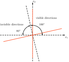
Figure 3. Illustration of the experimental setup and the corresponding visible/invisible directions according to the theory in Section 2. The red lines indicate the possible artifact directions.

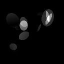
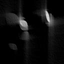
Figure 4. Two numerical reconstructions using FBP and U-net. Each row shows one example. Left: the original image. Middle: the FBP reconstruction. Right: the U-net reconstruction

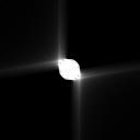
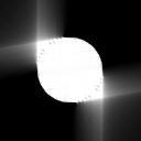
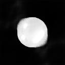
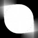
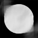
Figure 5. Numerical test of the stability condition in (7). Each row shows one example. Left: the original image. Middle: the FBP reconstruction. Right: the U-net reconstruction

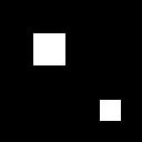
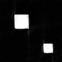
Figure 6. Left: the original image. Middle: the FBP reconstruction. Right: the U-net reconstruction

References

- [1] S. Barutcu, S. Aslan, A. Katsaggelos, D. Gürsoy. Limited-angle computed tomography with deep image and physics priors. Scientific Reports 11, no. 1 (2021): 17740.
- [2] T. Bubba, G. Kutyniok, M. Lassas, M. März, W. Samek, S. Siltanen, V. Srinivasan. Learning the invisible: a hybrid deep learning-shearlet framework for limited angle computed tomography. Inverse Problems, 35(6), 064002, 2019.
- [3] T. Bubba, M. Galinier, L. Ratti, M. Lassas, M. Prato, S. Siltanen. Deep neural networks for inverse problems with pseudodifferential operators: an application to limited-angle tomography. SIAM Journal on Imaging Science, 14(2) (2021): 470-505.
- [4] M. Davison. The ill-conditioned nature of the limited angle tomography problem. SIAM Journal on Applied Mathematics 43.2 (1983): 428-448.
- [5] T. Germer, J. Robine, S. Konietzny, S. Harmeling, T. Uelwer. Limited-angle tomography reconstruction via deep end-to-end learning on synthetic data. Applied Mathematics for Modern Challenges 1, no. 2 (2023): 126-142.
- [6] A. Goy, G. Rughoobur, S. Li, K. Arthur, A. Akinwande, G. Barbastathis. High-resolution limited-angle phase tomography of dense layered objects using deep neural networks. Proceedings of the National Academy of Sciences 116, no. 40 (2019): 19848-19856.
- [7] J. Gu, J. Ye. Multi-scale wavelet domain residual learning for limited-angle CT reconstruction. arXiv:1703.01382 (2017).
- [8] Y. Huang, T. Würfl, K. Breininger, L. Liu, G. Lauritsch, A. Maier. Some investigations on robustness of deep learning in limited angle tomography. In Medical Image Computing and Computer Assisted Intervention–MICCAI 2018: 21st International Conference, Granada, Spain, September 16-20, 2018, Proceedings, Part I, pp. 145-153. Springer International Publishing, 2018.
- [9] F. Natterer. The Mathematics of Computerized Tomography. Society for Industrial and Applied Mathematics, 2001.
- [10] T. Quinto. Singularities of the X-ray transform and limited data tomography in and . SIAM J. Math. Anal. 24 1215-25, 1993.
- [11] T. Quinto. Artifacts and visible singularities in limited data X-ray tomography. Sens. Imaging 18, 1-14, 2017.
- [12] S. Rautio, R. Murthy, T. Bubba, M. Lassas, S. Siltanen. Learning a microlocal prior for limited-angle tomography. arXiv:2201.00656 (2021).
- [13] O. Ronneberger, P. Fischer, T. Brox, U-net: Convolutional networks for biomedical image segmentation, International Conference on Medical image computing and computer-assisted intervention. Springer, 2015, pp. 234–241.
- [14] P. Stefanov, G. Uhlmann. Microlocal analysis and integral geometry. Book in progress.
- [15] https://github.com/megalinier/PsiDONet