Bayesian multi-exposure image fusion for robust
high dynamic range ptychography

Abstract

Image information is restricted by the dynamic range of the detector, which can be addressed using multi-exposure image fusion (MEF). The conventional MEF approach employed in ptychography is often inadequate under conditions of low signal-to-noise ratio (SNR) or variations in illumination intensity. To address this, we developed a Bayesian approach for MEF based on a modified Poisson noise model that considers the background and saturation. Our method outperforms conventional MEF under challenging experimental conditions, as demonstrated by the synthetic and experimental data. Furthermore, this method is versatile and applicable to any imaging scheme requiring high dynamic range (HDR).

1 Introduction

Detectors can only capture signals whose intensities are within the limits of their dynamic range. To surpass the limits of a detector, we can employ a multi-exposure image fusion (MEF) approach (Xu et al., 2022) by acquiring images at different exposure times ranging from under- to overexposed and fusing them into a single high dynamic range (HDR) image. Many MEF algorithms have been proposed (Zhang, 2021; Xu et al., 2022) with some adoption in microscopy (Yin et al., 2015; Singh et al., 2022; Liu et al., 2023). In coherent diffractive imaging (CDI), use of the aforementioned HDR image fusion algorithms has been limited (Baksh et al., 2016; Rose et al., 2018; Lo et al., 2018), predominantly relying on a similar approach referred to as the conventional MEF method in this work. Instead, experimental techniques based on wavefront modulation have been introduced to relax the dynamic range requirements (Zhang et al., 2016; Odstrčil et al., 2019; Eschen et al., 2024).

Ptychography, a scanning CDI method, has gained popularity as a ”lensless” computational imaging scheme allowing for simultaneous phase microscopy and wavefront sensing (Maiden & Rodenburg, 2009; Rodenburg & Maiden, 2019). It involves laterally moving a thin specimen across localized illumination while recording a series of diffraction patterns. By leveraging the overlap between adjacent scan positions, the captured diffraction data can be transformed into complex-valued reconstructions of the specimen and illumination wavefront using a phase-retrieval algorithm (Fig. 1a). The exposure time is a critical parameter for the acquisition of diffraction patterns. Photons diffracted towards large angles tend to exhibit lower intensities, resulting in a poorer signal-to-noise ratio (SNR). These photons carry high-spatial frequency information and are usually accessible through measurements with longer acquisition times, which may result in saturation of the pixels at the center of the diffraction patterns. Therefore, MEF (Fig. 1b) can be employed as a preprocessing step in ptychography to achieve a diffraction-limited resolution.

We briefly review the conventional MEF strategy (Baksh et al., 2016; Rose et al., 2018) before presenting our solution. For every scan position, multiple diffraction patterns $n_{i}(\boldsymbol{q})$ are recorded for varying acquisition times $t_{i}$ ($i=1,\ldots,K$), where $K$ denotes the number of acquisitions and $\boldsymbol{q}$ represents the pixel index. The background estimate $b_{i}(\boldsymbol{q})$ characterizes camera readout noise. A simple correction for background noise is the subtraction from the diffraction patterns $n_{i}^{+}(\boldsymbol{q}):=\max{\left(0,n_{i}(\boldsymbol{q})-b_{i}(\boldsymbol{q})\right)}$, where the max operation enforces nonnegativity. For every acquisition time $t_{i}$, there is an associated flux factor $c_{i}\approx t_{i}$. These patterns are then fused together into an estimated diffraction intensity $\mathcal{I}(\boldsymbol{q})$ based on maximum likelihood estimation (MLE) under the assumption of Poisson noise (see supplementary section B):

$$\mathcal{I}(\boldsymbol{q}) =\frac{\sum_{i}w_{i}(\boldsymbol{q})n_{i}^{+}(\boldsymbol{q})}{\sum_{i}w_{i}(\boldsymbol{q})c_{i}(\boldsymbol{q})},$$ (1)

$$\text{where},w_{i}(\boldsymbol{q}) =\begin{cases}1,&\text{$\boldsymbol{q}$ is not saturated}\\ 0,&\text{$\boldsymbol{q}$ is saturated}\end{cases}$$

Pixel-wise binary weight $w_{i}(\boldsymbol{q})$ ensures that only unsaturated data are used for the fusion process. Even if the exposure time is accurately known, conventional MLE suffers from several shortcomings, especially under low-SNR conditions. The background subtraction procedure clips negative values to zero, resulting in a loss of information. The $\max$ operation also introduces nonlinearity into intensity estimation, leading to a potential bias (Seifert et al., 2023). Additionally, this approach ignores saturated data, contributing to another source of information loss and leading to a suboptimal fusion result. Moreover, the flux factors $c_{i}$ may not be known accurately. In the case of probe intensity fluctuations (Odstrcil et al., 2016) or if the detector behaves nonlinearly under varying exposure times (Shafie et al., 2009), the conventional approach relies on a heuristic estimate of the flux factors, which affects the quality of fusion. In addition, recognizing the advantage of modifying the optical intensity, especially by increasing it while adjusting the camera exposure times, can prove beneficial for faster data acquisition. In this case, the uncertainty in $c_{i}$ will increase, introducing systematic errors in the fused data, thereby significantly affecting phase retrieval.

To tackle these issues and achieve robust HDR imaging in ptychography, this letter proposes a principled Bayesian approach to multi-exposure image fusion which we refer to here as the Bayesian MEF method. We start by explaining our probabilistic model, followed by demonstrating simulation results under low SNR conditions, assuming fixed and accurately known flux factors. Subsequently, we show the efficacy of our approach by using experimental data in a high SNR, and high photon count setting, where the flux factors are only heuristically known.

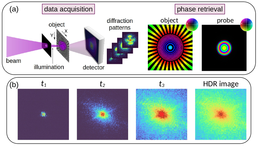
Figure 1: (a) Principle of conventional ptychography from data acquisition to phase retrieval. (b) Diffraction patterns recorded at increasing exposure times (bright red pixels are saturated) and fused to achieve a high dynamic range (HDR) image.

2 Bayesian MEF

At the core of a Bayesian approach is the likelihood, a probabilistic model for the data. Here, the model must account for two effects: (a) background noise and (b) saturation owing to overexposure. Suppose we ignore the background noise and saturation effects. In that case, an appropriate likelihood for the $i$-th exposure is a Poisson distribution with mean $c_{i}\mathcal{I}(\boldsymbol{q})$, i.e. $n_{i}(\boldsymbol{q})\sim\text{Poi}\left(c_{i}\mathcal{I}(\boldsymbol{q})\right)$ where $\sim$ denotes ”follows the distribution” (Thibault & Guizar-Sicairos, 2012). The second component of the Bayesian model is the prior. We assume a Gamma distribution as a prior with shape and scale parameters $\alpha_{\mathcal{I}}$ and $\beta_{\mathcal{I}}$. This choice encodes the assumption that $\mathcal{I}$ is non-negative and constant on average, $\mathcal{I}(\boldsymbol{q})\approx\alpha_{\mathcal{I}}/\beta_{\mathcal{I}}$, and the fluctuations in $\mathcal{I}$ are on the order of $\alpha_{\mathcal{I}}/\beta_{\mathcal{I}}^{2}$ (Gelman et al., 2013). In case we have more detailed prior knowledge about $\mathcal{I}$, it can be incorporated by letting $\alpha_{\mathcal{I}}$ and $\beta_{\mathcal{I}}$ depend on pixel location $\boldsymbol{q}$. We also assume gamma priors for the unknown flux factors $c_{i}$ where the hyperparameters $\alpha_{i},\beta_{i}$ are typically chosen such that the expected flux factor equals the acquisition time $\alpha_{i}/\beta_{i}=t_{i}$. The conditional posterior distributions for $\mathcal{I}(\boldsymbol{q})$ and $c_{i}$ are also gamma distributions. The model parameters can be estimated by iterating over the updates

$$c_{i}^{(k+1)} =\frac{\alpha_{i}+\sum_{\boldsymbol{q}}n_{i}(\boldsymbol{q})}{\beta_{i}+\sum_{\boldsymbol{q}}\mathcal{I}^{(k)}(\boldsymbol{q})},$$ (2)

$$\mathcal{I}^{(k+1)}(\boldsymbol{q}) =\frac{\alpha_{\mathcal{I}}+\sum_{i}n_{i}(\boldsymbol{q})}{\beta_{\mathcal{I}}+\sum_{i}c_{i}^{(k+1)}}$$

with iteration index denoted by superscript $(k)$. The derivation of the updates in Eq. (2) and the choice of hyperparameters $\alpha_{\mathcal{I}},\beta_{\mathcal{I}}$, etc., are provided in the supplementary section C.1. For $\alpha_{\mathcal{I}}=\beta_{\mathcal{I}}=0$, the estimate for $\mathcal{I}(\boldsymbol{q})$ matches the maximum-likelihood estimate for the unsaturated pixels in Eq. (1).

To model the readout noise, we consider the mean $c_{i}\mathcal{I}(\boldsymbol{q})$ to be shifted by the background mean $b_{i}(\boldsymbol{q})$ such that $n_{i}(\boldsymbol{q})\sim\text{Poi}\left(c_{i}\mathcal{I}(\boldsymbol{q})+b_{i}(\boldsymbol{q})\right)$. Since the sum of two Poisson distributions is again a Poisson distribution with both means added together, the data can be interpreted as the sum of the background counts generated from $\text{Poi}\left(b_{i}(\boldsymbol{q})\right)$ and noisefree counts $n_{\mathcal{I}i}(\boldsymbol{q})\sim\text{Poi}\left(c_{i}\mathcal{I}(\boldsymbol{q})\right)$. Only the sum of the background and noisefree counts is observed; however, $n_{\mathcal{I}i}(\boldsymbol{q})$ can be estimated from $n_{i}(\boldsymbol{q})$. The conditional posterior of the noisefree counts is a binomial distribution (see supplementary section C.2), and their expected values are

$$\mathbb{E}[n_{\mathcal{I}i}(\boldsymbol{q})\mid\mathcal{I}(\boldsymbol{q}),c_{i},b_{i}(\boldsymbol{q})]=\frac{c_{i}\mathcal{I}(\boldsymbol{q})}{c_{i}\mathcal{I}(\boldsymbol{q})+b_{i}(\boldsymbol{q})}n_{i}(\boldsymbol{q})\,.$$ (3)

These are fractions of the observed counts $n_{i}(\boldsymbol{q})$, which differ from estimating $n_{\mathcal{I}i}$ by subtracting the background.

To take the saturated pixels into account, we assume that the data $n_{i}(\boldsymbol{q})$ are censored at the detector threshold ${n^{*}}$ meaning that they are clipped at a maximum value of ${n^{*}}$. The likelihood is a (right-) censored Poisson distribution (i.e., the right tail of the Poisson distribution is not observed). Let $\nu_{i}(\boldsymbol{q})$ denote the latent uncensored counts, $\nu_{i}(\boldsymbol{q})\sim\text{Poi}\left(c_{i}\mathcal{I}(\boldsymbol{q})+b_{i}(\boldsymbol{q})\right)$ then, the observed data can be modeled as $n_{i}(\boldsymbol{q})=\nu_{i}(\boldsymbol{q})$ if $\nu_{i}(\boldsymbol{q})<{n^{*}}$ (or equivalently, $w_{i}(\boldsymbol{q})=1$), and $n_{i}(\boldsymbol{q})={n^{*}}$ if $\nu_{i}(\boldsymbol{q})\geq{n^{*}}$ (or $w_{i}(\boldsymbol{q})=0$). If we know $\nu_{i}(\boldsymbol{q})$, then parameter estimation would simplify to background removal under the Poisson model, as in Eq. (3). However, since we do not observe the uncensored counts directly, we have to estimate them. This can be achieved with conditional posteriors

$$\nu_{i}(\boldsymbol{q}) \sim\begin{cases}\text{TruncPoi}\left(c_{i}\mathcal{I}(\boldsymbol{q})+b_{i}(\boldsymbol{q}),{n^{*}}-1\right),\!\!&w_{i}(\boldsymbol{q})=0\\ \text{Poi}\left(c_{i}\mathcal{I}(\boldsymbol{q})+b_{i}(\boldsymbol{q})\right),&w_{i}(\boldsymbol{q})=1\end{cases}$$ (4)

$$\nu_{\mathcal{I}i}(\boldsymbol{q}) \sim\text{Binomial}\left(\nu_{i}(\boldsymbol{q}),\frac{c_{i}\mathcal{I}(\boldsymbol{q})}{c_{i}\mathcal{I}(\boldsymbol{q})+b_{i}(\boldsymbol{q})}\right)$$

$$\mathcal{I}(\boldsymbol{q}) \sim\text{Gamma}\bigl{(}\alpha_{\mathcal{I}}+\sum_{i}\nu_{\mathcal{I}i}(\boldsymbol{q}),\beta_{\mathcal{I}}+\sum_{i}c_{i}\bigr{)}$$

where $\nu_{\mathcal{I}i}(\boldsymbol{q})$ are the noisefree contributions to the uncensored counts $\nu_{i}(\boldsymbol{q})$ and TruncPoi denotes the truncated Poisson distribution (Plackett, 1953). We can now employ the expectation-maximization (EM) (Dempster et al., 1977) algorithm to estimate the fused diffraction pattern $\mathcal{I}$ (see supplementary section C.3 for details). The E-step gives the expectation of $\nu_{i}$, allowing us to estimate $\nu_{\mathcal{I}i}$ and the M-step maximizes our estimate of $\mathcal{I}$ in the presence of incomplete data.

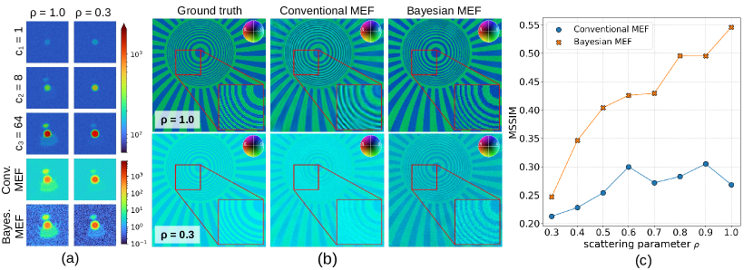
Figure 2: (a) Synthetic diffraction patterns (log-scale) for a particular scan position under strong scattering ($\rho=1.0$) and weak scattering ($\rho=0.3$) corresponding to different flux factors $c_{i}$. The third acquisition ($c_{3}=64.0$) exhibits saturation (bright red pixels). The data is then fused with conventional and Bayesian MEF methods. (b) Comparing ptychographic reconstructions (amplitude and phase) of the ground truth with MEF fused result from the synthetic data for $\rho=1.0$ (top-row) and $\rho=0.3$ (bottom-row). (c) Evaluating the mean structural similarity index (MSSIM) for reconstructed phase with data generated by varying $\rho$.

Algorithm 1 summarizes the Bayesian MEF updates. The key steps are: Estimation of the uncensored counts $\nu_{i}$ via their expected values under the truncated Poisson distribution (line 4), background removal (line 5) analogous to Eq. (3), updating the flux factors (line 6), and estimation of the fused pattern (line 7). This procedure iteratively reduces the measured readout noise in addition to estimating the saturated pixels for correcting flux factors and fusing the diffraction patterns.

Algorithm 1 Bayesian MEF algorithm

1:  Initialize $\alpha_{\mathcal{I}}=\beta_{\mathcal{I}}=0.001$, $\alpha_{i}=1.0$ and $\beta_{i}=t_{i}^{-1}$

2:  Initialize $c_{i}^{(0)}=t_{i}$,   $\mathcal{I}^{(0)}=\frac{\alpha_{\mathcal{I}}+\sum_{i}w_{i}n_{i}}{\beta_{\mathcal{I}}+\sum_{i}w_{i}t_{i}}$

3:  repeat

4:     $\nu_{i}^{(k+1)}\leftarrow w_{i}n_{i}+\left(1-w_{i}\right)\mathbb{E}[\nu_{i}|c_{i}^{(k)}\mathcal{I}^{(k)}+b_{i},{n^{*}}-1]$

5:     $\nu_{\mathcal{I}i}^{(k+1)}\leftarrow\frac{c_{i}^{(k)}\mathcal{I}^{(k)}}{c_{i}^{(k)}\mathcal{I}^{(k)}+b_{i}}\scriptsize{\nu_{i}^{(k+1)}}$

6:     $c_{i}^{(k+1)}\leftarrow\frac{\alpha_{i}+\sum_{\boldsymbol{q}}\nu_{\mathcal{I}i}^{(k+1)}(\boldsymbol{q})}{\beta_{i}+\sum_{\boldsymbol{q}}\mathcal{I}^{(k)}(\boldsymbol{q})}$

7:     $\mathcal{I}^{(k+1)}\leftarrow\frac{\alpha_{\mathcal{I}}+\sum_{i}\nu_{\mathcal{I}i}^{(k+1)}}{\beta_{\mathcal{I}}+\sum_{i}c_{i}^{(k+1)}}$

8:     $k\leftarrow k+1$

9:  until converge

3 Simulations for low SNR data with known flux factors

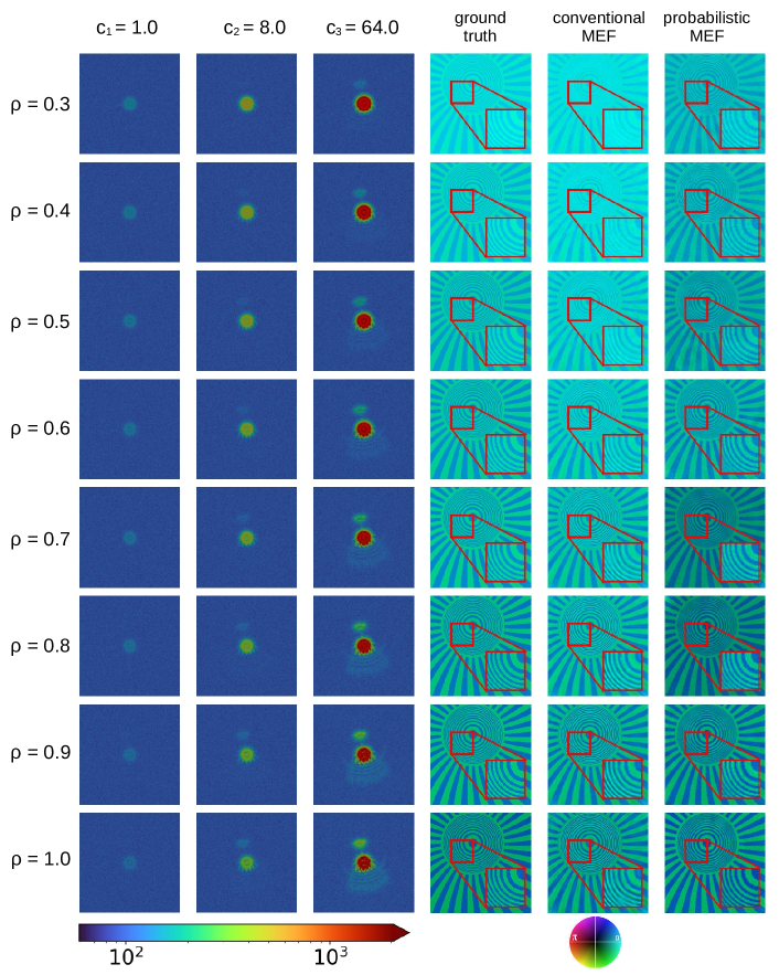
Figure 5: Every row corresponds to synthetic data (log-scale) with ptychographic reconstruction results for scattering parameter $\rho$. The diffraction patterns recorded at varying flux factors $c_{i}$ are fused with conventional and Bayesian MEF methods and the ptychographic reconstruction results are compared with the ground truth.

To study the performance of Bayesian MEF, we considered synthetic data in a low-SNR setting. We fixed the flux factors $c_{i}=t_{i}$ and did not estimate them. To simulate a low-SNR condition, we considered a weakly scattering specimen. The signal from the specimen in the far-field diffraction pattern is not just weak but also dominated by the unscattered probe, increasing the shot noise and thereby lowering the effective SNR (see supplementary section D.1). The ptychographic reconstruction of these data is usually more challenging (Dierolf et al., 2010). In general, a phase object is given by $O(\boldsymbol{q})=\exp{\big{(}i\phi(\boldsymbol{q})\big{)}}$ where $\rho\approx\max\big{(}\phi(\boldsymbol{q})\big{)}$ denotes the maximum phase. Smaller values of $\rho$ result in weaker scattering, corresponding to a weakly phase-modulating specimen. To systematically study the impact on ptychographic reconstructions, we simulated the data by varying $\rho$ from weakly scattering $\rho=0.3$ to strongly scattering $\rho=1.0$. For a given $\rho$, the diffraction patterns are simulated using our forward model $n_{i}(\boldsymbol{q})\sim\text{Poi}\left(c_{i}\mathcal{I}(\boldsymbol{q})+b_{i}(\boldsymbol{q})\right)$ where the additive background is drawn from the Gaussian distribution $b_{i}(\boldsymbol{q})\sim\mathcal{N}(\mu_{b},\sigma^{2}_{b})$ (Seifert et al., 2023). Usually, the background counts are a small fraction of the actual data and remain fairly constant with low spatial variance. Therefore, we choose $\mu_{b}=100$ and $\sigma^{2}_{b}=0.8$. We set $c_{i}$ to 1, 8, and 64, corresponding to maximum photon counts of $2^{7},2^{10}$ and $2^{13}$, respectively. The data was censored at a threshold of $2^{11}$ causing saturation mainly in the third acquisition. The simulated diffraction patterns are shown in Fig. 2a, where acquisitions for a specific scan position were generated for $\rho=1.0$ and $\rho=0.3$. For the third acquisition ($c_{3}=64$), the number of saturated pixels was $\approx 2.3$ times higher for $\rho=0.3$ than for $\rho=1.0$, further increasing the level of uncertainty in the fusion of data from the weakly scattering specimen. For each exposure time, we repeated the measurement six times, fusing $18$ measurements per scan point. Utilizing fused data from all scan positions, we employed the momentum acceleration (mPIE) (Maiden et al., 2017) phase retrieval algorithm implemented in the open-source package PtyLab (Loetgering et al., 2023). Fig. 2b compares the impact of the MEF methods on the reconstruction of a spokes target as our phase object. The reconstruction quality was significantly better with the Bayesian MEF method for strongly as well as weakly scattering data. Supplementary Fig. 5 compares the results for $\rho$ varying from $0.3$ to $1.0$ showing improved reconstructions for all cases. These results are corroborated by evaluating the mean structural similarity (MSSIM) index (Wang et al., 2004) for phase reconstructions by varying $\rho$ (see Fig. 2c). Supplementary section D.2 contains more details on the MSSIM metric as well as its use. As seen here, our method consistently shows higher MSSIM values for all values of $\rho$, whereas the improvement in the conventional case remains stagnant even for $\rho$ corresponding to strongly scattering ($\rho=1.0$) data.

4 Experimental demonstration for high SNR data with heuristic flux factors

The tests with synthetic data utilized the known flux factors $c_{i}$. However, these may or may not be known from an experiment. In the following experimental tests, we have a high SNR and high photon count setting; however, the flux factors are only heuristically known. We demonstrate that the fusion results from the conventional case become unreliable when the flux factors deviate significantly from the actual values. One such case is when the illumination intensity also varies with camera exposure time. In this case, we only have access to heuristic estimate $c_{i}^{heu}$. It can be calculated by summing the uncensored data for every acquisition and dividing it by the sum of uncensored data for a fixed acquisition. For example, out of $K$ acquisitions, the fixed acquisition could be the middle one $i=K/2$. The Bayesian MEF approach, outlined in algorithm 1, should iteratively correct the heuristic flux factors by setting $c_{i}^{(0)}=c_{i}^{heu.}$. To test this, we constructed a conventional ptychography setup in transmission geometry. A coherent laser source from SuperK COMPACT, offering manual adjustment of the laser power in percentage was employed. We chose a wavelength of $625\,nm$, a probe size of $400\,\mu m$, and used an unstained histological mouse section as our test object. Diffraction data was recorded at $500$ scan positions using a Lucid CMOS camera with a $12$ bit analog-to-digital converter (ADC) and a binning factor of $8$, allowing a maximum of $2^{18}$ counts.

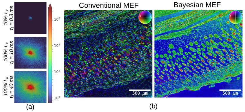
Figure 3: (a) Diffraction patterns recorded with varying laser power $L_{p}$ in percentage and camera acquisition times $t_{i}$. The second and the third acquisitions are overexposed. (b) Ptychographic reconstructions using the two MEF methods.

For additional experimental details, please refer to supplementary section E. We recorded three acquisitions by varying the exposure time and the laser power in percentage (refer to Fig. 3a). Each acquisition was repeated thrice, necessitating the fusion of nine diffraction patterns per scan. For each acquisition, $150$ dark-frame measurements were recorded and averaged. For the conventional MEF case, we applied the background subtraction procedure to the diffraction patterns and estimated the flux factors heuristically. Subsequently, the conventional MEF method was applied, resulting in a largely unsuccessful ptychographic reconstruction, as depicted in the left panel of Fig. 3b. However, our method corrects the heuristic flux factors and estimates fused patterns, leading to a high-quality ptychographic reconstruction (see Fig. 3b, right panel). It is expected that both MEF methods yield comparable results in a high SNR and high photon count scenario, where flux factors are accurately known. This is verified by utilizing the corrected fluxes from our method and using them for the conventional MEF case, leading to visually indistinguishable reconstructions (see Fig. 4).

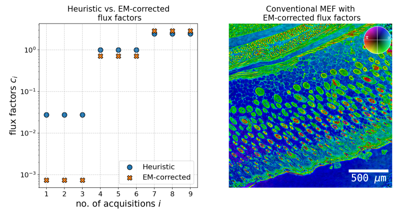
Figure 4: (a) Heuristic flux factors are corrected by our EM algorithm (shown in log-scale) for the nine measurements (each acquisition repeated thrice) for every scan position. (b) Conventional MEF reconstruction that used the corrected fluxes from our EM algorithm.

5 Summary

We introduced a Bayesian approach for MEF that incorporates image formation statistics with priors in a principled manner. Our findings illustrate enhanced HDR phase retrieval, particularly under challenging conditions such as low SNR or variations in illumination intensity. It can also be noted that conventional MEF is merely a special case of the Bayesian MEF method, which is verified when both methods perform equivalently with known flux factors in a high SNR regime. Currently, MEF is a preprocessing step for ptychography, and an extension of this work could be the integration of our Bayesian model directly into a ptychography framework based on automatic differentiation (AD) (Kandel et al., 2019), potentially further enhancing robustness in HDR ptychographic reconstructions. Additionally, exploring physics-informed priors could improve the estimation in scenarios with limited data or expedite algorithmic convergence.

In summary, the results showcased in this study suggest noteworthy advancements in the field of computational imaging. Our work shows promise for imaging challenging weakly scattering specimens or when access to high-quality detectors at extreme wavelengths (Thibault et al., 2008; Loetgering et al., 2022) is either limited or expensive. Furthermore, Bayesian MEF extends its utility beyond CDI to encompass any imaging scheme that necessitates HDR treatment.

Data Availability Statement

The data used in this work and the algorithms implemented as a software package can be found in Ref. (Kodgirwar et al., 2024).

Appendix A Mathematical Notation

• Iverson bracket:

  $$\llbracket A\rrbracket=\begin{cases}1,&\text{$A$ is true}\\ 0,&\text{$A$ is false}\end{cases}$$

• Expectation:

  $$\mathbb{E}[f]=\int f(x)\,p(x)\,dx$$

  is the expected value of quantity $f$ under the probability distribution $p$. Special cases are the mean

  $$\mathbb{E}[x]=\int x\,p(x)\,dx$$

  and variance

  $$\text{var}[x]=\mathbb{E}\big{[}(x-\mathbb{E}[x])^{2}\big{]}=\mathbb{E}[x^{2}]-\left(\mathbb{E}[x]\right)^{2}\,.$$

  If $p(x\mid\theta)$ is a conditional probability distribution with parameter(s) $\theta$, then the expectations depend on $\theta$ which we make explicit by the following notation:

  $$\mathbb{E}[f\mid\theta]=\int f(x)\,p(x\mid\theta)\,dx$$

• “Follows”: The tilde symbol “$\sim$” indicates that a quantity $x$ follows a particular probability distribution $p$:

  $$x\sim p(x)$$

• Parameters of the image model:

  $\boldsymbol{q}$:

  detector pixel coordinates

  $t_{i}$:

  camera acquisition times (with $i=1,\ldots,K$ where $K$ is the number of acquisitions)

  $n_{i}(\boldsymbol{q})$:

  diffraction patterns acquired during $t_{i}$ for a given scan position

  $b_{i}(\boldsymbol{q})$:

  dark frame measurements acquired during $t_{i}$

  $\mathcal{I}(\boldsymbol{q})$:

  fused image / diffraction pattern

  $w_{i}(\boldsymbol{q})$:

  binary weight that is equal to $1$ for unsaturated pixels, $0$ otherwise

  $c_{i}$:

  flux rate associated with acquisition time $t_{i}$

• Poisson distribution:

  $$\text{Poi}\left(n;\lambda\right)=\frac{\lambda^{n}}{n!}e^{-\lambda},\quad\lambda>0,\quad n=0,1,2,\ldots$$

  with rate $\lambda$ for counts $n$.

• $k$-truncated Poisson distribution:

  $$\text{TruncPoi}\left(n;\lambda,k\right)\propto\text{Poi}\left(n;\lambda\right)\,\llbracket n>k\rrbracket$$

  This is a Poisson distribution with rate $\lambda$ where the counts are $n=k+1,k+2,\ldots$. The normalization constant is:

  $$\sum_{n>k}\text{Poi}\left(n;\lambda\right)=1-\sum_{n\leq k}\text{Poi}\left(n;\lambda\right)=1-e^{-\lambda}\sum_{n=0}^{k}\frac{\lambda^{n}}{n!}\,.$$

• Gamma distribution:

  $$\text{Gamma}\left(x;\alpha,\beta\right)=\frac{\beta^{\alpha}}{\Gamma(\alpha)}x^{\alpha-1}e^{-\beta x},\quad x,\alpha,\beta\geq 0$$

  where $\Gamma(\cdot)$ is the Gamma function. The parameter $\alpha$ is the shape parameter, $\beta$ is the rate parameter. The mean and variance of a Gamma variable are:

  $$\mathbb{E}[x]=\frac{\alpha}{\beta},\quad\text{var}[x]=\frac{\alpha}{\beta^{2}}\,.$$

• Binomial distribution:

  $$\text{Binomial}(k;n,p)=\binom{n}{k}\,p^{k}\,(1-p)^{n-k}=\frac{n!}{k!(n-k)!}\,p^{k}\,(1-p)^{n-k}$$

  calculates the probability of getting exactly $k$ successes in $n$ trials ($k\leq n$) with a probability $p\in[0,1]$ of success in each trial. The expected number of counts is

  $$\mathbb{E}[k]=p\,n\,.$$

Appendix B Conventional multi-exposure image fusion

Photon counts on a detector can be assumed to follow a Poisson distribution. Under the assumption of independent and identically distributed (i.i.d.) counts, the likelihood of acquiring a diffraction pattern $n(\boldsymbol{q})$ given some true diffraction intensity $\mathcal{I}(\boldsymbol{q})$ is

$$\Pr(n(\boldsymbol{q})\mid\mathcal{I}(\boldsymbol{q}))=\text{Poi}\left(n(\boldsymbol{q});\mathcal{I}(\boldsymbol{q})\right)=\frac{[\mathcal{I}(\boldsymbol{q})]^{n(\boldsymbol{q})}}{n(\boldsymbol{q})!}e^{-\mathcal{I}(\boldsymbol{q})}\,.$$ (5)

In MEF, we measure diffraction patterns $n_{i}(\boldsymbol{q})$ by increasing the optical intensity by some flux factor $c_{i}$ which is proportional to the acquisition times $t_{i}$. Under the assumption that $c_{i}\approx t_{i}$, we can rewrite the likelihood of observing $n_{i}(\boldsymbol{q})$ counts at pixel $\boldsymbol{q}$ as

$$\Pr(n_{i}(\boldsymbol{q})\mid\mathcal{I},c_{i})=\text{Poi}\left(n_{i}(\boldsymbol{q});c_{i}\mathcal{I}(\boldsymbol{q})\right)=\frac{[c_{i}\mathcal{I(\boldsymbol{q})}]^{n_{i}(\boldsymbol{q})}}{n_{i}(\boldsymbol{q})!}e^{-c_{i}\mathcal{I}(\boldsymbol{q})}\,.$$ (6)

We will occasionally drop the pixel dependence $\boldsymbol{q}$ for convenience. The log likelihood $\ell_{i}$ for the fused image $\mathcal{I}$ resulting from the $i$-th acquition can be written as

$$\ell_{i}(\mathcal{I})=\displaystyle\sum_{\boldsymbol{q}}\big{\{}n_{i}(\boldsymbol{q})\log[c_{i}\mathcal{I}(\boldsymbol{q})]-c_{i}\mathcal{I}(\boldsymbol{q})\big{\}}\,.$$ (7)

By incorporating only unsaturated pixels via the pixel-wise weight factor $w_{i}(\boldsymbol{q})$, and summing over diffraction patterns $n_{i}(\boldsymbol{q})$, the total log-likelihood becomes,

$$\ell(\mathcal{I})=\displaystyle\sum_{i}\sum_{\boldsymbol{q}}\big{\{}w_{i}(\boldsymbol{q})n_{i}(\boldsymbol{q})\log[c_{i}\mathcal{I}(\boldsymbol{q})]-w_{i}(\boldsymbol{q})c_{i}\mathcal{I}(\boldsymbol{q})\big{\}}\,.$$ (8)

The maximum likelihood estimate (MLE) of $\mathcal{I}$ is obtained by maximizing the log likelihood:

$$\mathcal{I}_{\text{MLE}}=\underset{\mathcal{I}}{\operatorname*{arg\,max}}\,\ell(\mathcal{I})\,.$$

The MLE can be computed by setting the gradient of $\ell$ to zero:

$$\frac{\partial\ell(\mathcal{I})}{\partial I(\boldsymbol{q})}=\sum_{i}\frac{w_{i}(\boldsymbol{q})\,n_{i}(\boldsymbol{q})}{\mathcal{I}(\boldsymbol{q})}-\sum_{i}w_{i}(\boldsymbol{q})c_{i}\overset{!}{=}0\,.$$

Solving this for $\mathcal{I}$ the fused MEF result is now given as

$$\mathcal{I}_{\text{MLE}}(\boldsymbol{q})=\frac{\sum_{i}w_{i}(\boldsymbol{q})\,n_{i}(\boldsymbol{q})}{\sum_{i}w_{i}(\boldsymbol{q})\,c_{i}}\,.$$

After subtracting the dark frame measurements $b_{i}(\boldsymbol{q})$ from the diffraction patterns

$$n_{i}^{+}(\boldsymbol{q}):=\max{\big{(}0,n_{i}(\boldsymbol{q})-b_{i}(\boldsymbol{q})\big{)}}\,,$$

the conventional MEF result can be rewritten as

$$\mathcal{I}_{\text{MLE}}(\boldsymbol{q}) =\frac{\sum_{i}w_{i}(\boldsymbol{q})\,n_{i}^{+}(\boldsymbol{q})}{\sum_{i}w_{i}(\boldsymbol{q})\,c_{i}},\quad w_{i}(\boldsymbol{q})=\begin{cases}1,&\text{$\boldsymbol{q}$ is not saturated}\\ 0,&\text{$\boldsymbol{q}$ is saturated}\end{cases}$$ (9)

by replacing the raw counts $n_{i}(\boldsymbol{q})$ with the background-corrected counts $n_{i}^{+}(\boldsymbol{q})$.

Appendix C Bayesian multi-exposure image fusion

To derive Bayesian multi-exposure image fusion (MEF), we divide it in three parts. The first part focuses on considering the Poisson likelihood and deriving model parameters for fused data $\mathcal{I}(\boldsymbol{q})$ and $c_{i}$. In the next subsection, we assume that the Poisson data is corrupted with background, therefore modifying our likelihood to accommodate for this. We derive the model parameters under this situation. In the last subsection, we assume a right-(censored) Poisson distribution to model the saturated pixels along with the consideration of the background data.

C.1 Poisson data

The likelihood of observing $n_{i}(\boldsymbol{q})$ at pixel $\boldsymbol{q}$ is defined in Eq. 6. The likelihood over the entire dataset can be given as

$$\mathcal{L}(\mathcal{I},c)=\prod_{i}\prod_{\boldsymbol{q}}\left[c_{i}\mathcal{I}(\boldsymbol{q})\right]^{n_{i}(\boldsymbol{q})}e^{-c_{i}\mathcal{I}(\boldsymbol{q})}\,.$$ (10)

We now define prior distributions. For $c_{i}$, we assume a Gamma distribution as prior

$$\Pr(c_{i}\mid\alpha_{i},\beta_{i})=\text{Gamma}\left(c_{i};\alpha_{i},\beta_{i}\right)=\frac{\beta_{i}^{\alpha_{i}}}{\Gamma(\alpha_{i})}\,c_{i}^{\alpha_{i}-1}e^{-\beta_{i}c_{i}}$$ (11)

with the following properties

$$\mathbb{E}[c_{i}]=\frac{\alpha_{i}}{\beta_{i}},\quad\text{var}[c_{i}]=\frac{\alpha_{i}}{\beta_{i}^{2}}\,.$$ (12)

Similarly, our prior for $\mathcal{I}(\boldsymbol{q})$ is

$$\Pr(\mathcal{I}(\boldsymbol{q})\mid\alpha_{\mathcal{I}},\beta_{\mathcal{I}})=\text{Gamma}\left(\mathcal{I}(\boldsymbol{q});\,\alpha_{\mathcal{I}},\beta_{\mathcal{I}}\right)=\frac{\beta_{\mathcal{I}}^{\alpha_{\mathcal{I}}}}{\Gamma(\alpha_{\mathcal{I}})}\left[\mathcal{I}(\boldsymbol{q})\right]^{\alpha_{\mathcal{I}}-1}e^{-\beta_{\mathcal{I}}\mathcal{I}(\boldsymbol{q})}$$ (13)

The joint posterior is obtained by invoking Bayes’ rule:

$$\Pr(\mathcal{I}(\boldsymbol{q}),c_{i}\mid n_{i})\propto\Pr(n_{i}(\boldsymbol{q})\mid\mathcal{I}(\boldsymbol{q}),c_{i})\,\Pr(\mathcal{I}(\boldsymbol{q})\mid\alpha_{\mathcal{I}},\beta_{\mathcal{I}})\,\Pr(c_{i}\mid\alpha_{i},\beta_{i})$$ (14)

where the dependence on the hyperparameters $\alpha_{\mathcal{I}},\beta_{\mathcal{I}},\alpha_{i},\beta_{i}$ is omitted. Due to the conjugacy property, the conditional posterior distributions for $\mathcal{I}$ and $c_{i}$ will also be Gamma distributions. For $\Pr(\mathcal{I},\mid c_{i},n_{i})$, we have

$$\Pr(\mathcal{I}(\boldsymbol{q})\mid c_{i},n_{i})=\text{Gamma}\left(\mathcal{I}(\boldsymbol{q});\,\alpha_{\mathcal{I}}+\sum_{i}n_{i}(\boldsymbol{q}),\beta_{\mathcal{I}}+\sum_{i}c_{i}\right)$$ (15)

Similarly for $\Pr(c_{i}\mid\mathcal{I},n_{i})$, we have

$$\Pr(c_{i}\mid\mathcal{I},n_{i})=\text{Gamma}\left(c_{i};\,\alpha_{i}+\sum_{\boldsymbol{q}}n_{i}(\boldsymbol{q}),\beta_{i}+\sum_{\boldsymbol{q}}\mathcal{I}(\boldsymbol{q})\right)$$ (16)

Therefore, using the analytical expression for the expectation of the Gamma distribution, the model parameters can be estimated as,

$$\mathcal{I}^{(k+1)}(\boldsymbol{q}) =\mathbb{E}[\mathcal{I}(\boldsymbol{q})\mid c_{i}^{(k)}]=\frac{\alpha_{\mathcal{I}}+\sum_{i}n_{i}(\boldsymbol{q})}{\beta_{\mathcal{I}}+\sum_{i}c_{i}^{(k)}}\,\,,$$ (17)

$$c_{i}^{(k+1)} =\mathbb{E}[c_{i}\mid\mathcal{I}^{(k+1)}]=\frac{\alpha_{i}+\sum_{\boldsymbol{q}}n_{i}(\boldsymbol{q})}{\beta_{i}+\sum_{\boldsymbol{q}}\mathcal{I}^{(k+1)}(\boldsymbol{q})}$$

The expectation for a uniform Gamma prior of $\mathcal{I}(\boldsymbol{q})$ can be given as $\alpha_{\mathcal{I}}/\beta_{\mathcal{I}}=1$. To achieve this, we simply provide the same value for $\alpha_{\mathcal{I}}$ and $\beta_{\mathcal{I}}$. Here, we choose both of these values to be $10^{-3}$, which also avoids instability in the division. Since, we expect $c_{i}\approx t_{i}$, the prior expectation is then given as $\alpha_{i}/\beta_{i}=t_{i}$. For the special case of $\alpha_{i}=1$ which is the exponential distribution, $\beta_{i}=t_{i}^{-1}$.

C.2 Poisson data with background

To account for the background or readout noise, we assume the Poisson rate $c_{i}\mathcal{I}(\boldsymbol{q})$ is shifted by some background rate $b_{i}(\boldsymbol{q})$

$$n_{i}(\boldsymbol{q})\sim\text{Poi}\left(n_{i}(\boldsymbol{q});c_{i}\mathcal{I}(\boldsymbol{q})+b_{i}(\boldsymbol{q})\right)\,.$$ (18)

The model can be interpreted as observing the sum of the latent unobserved noisefree diffraction patterns $n_{\mathcal{I}i}(\boldsymbol{q})$ and background counts $n_{bi}(\boldsymbol{q})$.

$$\begin{split}&\text{Poi}\left(n_{i}(\boldsymbol{q});c_{i}\mathcal{I}(\boldsymbol{q})+b_{i}(\boldsymbol{q})\right)\\ &=\displaystyle\sum_{n_{\mathcal{I}i}(\boldsymbol{q}),n_{bi}(\boldsymbol{q})=0}^{\infty}\llbracket n_{i}(\boldsymbol{q})=n_{\mathcal{I}i}(\boldsymbol{q})+n_{bi}(\boldsymbol{q})\rrbracket\,\text{Poi}\left(n_{\mathcal{I}i}(\boldsymbol{q});c_{i}\mathcal{I}(\boldsymbol{q})\right)\text{Poi}\left(n_{bi}(\boldsymbol{q});b_{i}(\boldsymbol{q})\right)\,.\end{split}$$ (19)

This follows from the binomial theorem as

$$\sum_{k,l=0}^{\infty}\llbracket s=k+l\rrbracket\,\text{Poi}\left(k;x\right)\,\text{Poi}\left(l;y\right) =\sum_{k,l=0}^{\infty}\llbracket s=k+l\rrbracket\,\frac{x^{k}}{k!}\,\frac{y^{l}}{l!}e^{-(x+y)}$$

$$=e^{-(x+y)}\sum_{k=0}^{s}\frac{x^{k}}{k!}\,\frac{y^{s-k}}{(s-k)!}$$

$$=\frac{e^{-(x+y)}}{s!}\sum_{k=0}^{s}\binom{s}{k}x^{k}\,y^{s-k}$$

$$=\frac{e^{-(x+y)}}{s!}(x+y)^{s}=\text{Poi}\left(s;x+y\right)$$

To derive the conditional posterior of the latent counts, we note that the distribution $n_{\mathcal{I}i}(\boldsymbol{q})$ given $n_{i}(\boldsymbol{q})$ is

$$\Pr(n_{\mathcal{I}i}(\boldsymbol{q})\mid n_{i}(\boldsymbol{q}),\mathcal{I}(\boldsymbol{q}),c_{i},b_{i}(\boldsymbol{q}))=\frac{\Pr(n_{i}(\boldsymbol{q}),n_{\mathcal{I}i}(\boldsymbol{q})\mid\mathcal{I}(\boldsymbol{q}),c_{i},b_{i}(\boldsymbol{q}))}{\Pr(n_{i}(\boldsymbol{q})\mid\mathcal{I}(\boldsymbol{q}),c_{i},b_{i}(\boldsymbol{q}))}$$

We have for $\Pr(n_{i}(\boldsymbol{q}),n_{\mathcal{I}i}(\boldsymbol{q})\mid\mathcal{I}(\boldsymbol{q}),c_{i},b_{i}(\boldsymbol{q}))$

$$\Pr(n_{i},n_{\mathcal{I}i}\mid\mathcal{I},c_{i},b_{i}) =\sum_{n_{bi}=0}^{\infty}\llbracket n_{i}=n_{\mathcal{I}i}+n_{bi}\rrbracket\,\text{Poi}\left(n_{\mathcal{I}i};c_{i}\mathcal{I}\right)\text{Poi}\left(n_{bi};b_{i}\right)$$ (20)

$$=\frac{e^{-(c_{i}\mathcal{I}+b_{i})}}{n_{i}!}\binom{n_{i}}{n_{\mathcal{I}i}}\left(c_{i}\mathcal{I}\right)^{n_{\mathcal{I}i}}b_{i}^{n_{i}-n_{\mathcal{I}i}},$$

and $\Pr(n_{i}(\boldsymbol{q})\mid\mathcal{I}(\boldsymbol{q}),c_{i},b_{i}(\boldsymbol{q}))$

$$\Pr(n_{i}\mid\mathcal{I},c_{i},b_{i})=\text{Poi}\left(n_{i};c_{i}\mathcal{I}+b_{i}\right)=\frac{\left(c_{i}\mathcal{I}+b_{i}\right)^{n_{i}}}{n_{i}!}e^{-\left(c_{i}\mathcal{I}+b_{i}\right)}\,,$$ (21)

From Eq. 20 and Eq. 21, it follows that

$$\Pr(n_{\mathcal{I}i}\mid n_{i},\mathcal{I},c_{i},b_{i}) =\frac{e^{-(c_{i}\mathcal{I}+b_{i})}}{n_{i}!}\binom{n_{i}}{n_{\mathcal{I}i}}\left(c_{i}\mathcal{I}\right)^{n_{\mathcal{I}i}}b_{i}^{n_{i}-n_{\mathcal{I}i}}\biggl{/}\biggr{.}\frac{\left(c_{i}\mathcal{I}+b_{i}\right)^{n_{i}}}{n_{i}!}e^{-\left(c_{i}\mathcal{I}+b_{i}\right)}$$ (22)

$$=\binom{n_{i}}{n_{\mathcal{I}i}}\frac{\left(c_{i}\mathcal{I}\right)^{n_{\mathcal{I}i}}b_{i}^{n_{i}-n_{\mathcal{I}i}}}{(c_{i}\mathcal{I}+b_{i})^{n_{i}}}$$

$$=\text{Binomial}\left(n_{\mathcal{I}i};n_{i},\frac{c_{i}\mathcal{I}}{c_{i}\mathcal{I}+b_{i}}\right)$$

We record the aggregate counts $n_{i}(\boldsymbol{q})$ and if we were to measure dark frames $m_{ij}(\boldsymbol{q})$, i.e., repeat $J$ measurements per acquisition, we can write it as

$$m_{ij}(\boldsymbol{q})\sim\text{Poi}\left(\,\cdot\,;b_{i}(\boldsymbol{q})\right),\quad j=1,\ldots,J$$

We can assume the mean of the dark frames to be $\overline{m}_{i}(\boldsymbol{q})\approx b_{i}(\boldsymbol{q})$ and therefore the background rate $b_{i}(\boldsymbol{q})$ to be known for all acquisitions. We can summarize all the conditional posterior distributions as

$$\begin{split}\mathcal{I}(\boldsymbol{q})&\sim\text{Gamma}\left(\mathcal{I}(\boldsymbol{q});\,\alpha_{\mathcal{I}}+\sum_{i}n_{\mathcal{I}i}(\boldsymbol{q}),\beta_{\mathcal{I}}+\sum_{i}c_{i}\right)\\ n_{\mathcal{I}i}(\boldsymbol{q})&\sim\text{Binomial}\left(n_{\mathcal{I}i}(\boldsymbol{q});n_{i}(\boldsymbol{q}),\frac{c_{i}\mathcal{I}(\boldsymbol{q})}{c_{i}\mathcal{I}(\boldsymbol{q})+b_{i}(\boldsymbol{q})}\right)\end{split}$$ (23)

We can employ the expectation-maximization (EM) algorithm. In the expectation step (E-step), we find the expectation of the latent quantity $n_{\mathcal{I}i}(\boldsymbol{q})$. In the maximization step (M-step), we maximize our estimation of the fused diffraction pattern $\mathcal{I}(\boldsymbol{q})$.

$$n_{\mathcal{I}i}^{(k+1)}(\boldsymbol{q}) =\mathbb{E}[n_{\mathcal{I}i}(\boldsymbol{q})\mid\mathcal{I}^{(k)}(\boldsymbol{q})]=\frac{c_{i}\mathcal{I}^{(k)}(\boldsymbol{q})}{c_{i}\mathcal{I}^{(k)}(\boldsymbol{q})+b_{i}(\boldsymbol{q})}\,n_{i}(\boldsymbol{q})$$ (24)

$$\mathcal{I}^{(k+1)}(\boldsymbol{q}) =\mathbb{E}[\mathcal{I}(\boldsymbol{q})\mid n_{\mathcal{I}i}^{(k+1)}(\boldsymbol{q})]=\frac{\alpha_{\mathcal{I}}+\sum_{i}n_{\mathcal{I}i}^{(k+1)}(\boldsymbol{q})}{\beta_{\mathcal{I}}+\sum_{i}c_{i}}$$

C.3 Censored Poisson data with background

Now assume that the data are truncated at some censoring threshold ${n^{*}}$ such that the observed counts $n_{i}(\boldsymbol{q})$ are restricted to the range $[0,{n^{*}}]$. These data can be modeled as unrestricted counts $\nu_{i}(\boldsymbol{q})\in\mathbb{N}$

$$\nu_{i}(\boldsymbol{q})\sim\text{Poi}\left(\,\cdot\,;c_{i}\mathcal{I}(\boldsymbol{q})+b_{i}(\boldsymbol{q})\right)$$ (25)

that are only partially observed. If we knew all $\nu_{i}(\boldsymbol{q})$, then the estimation of $\mathcal{I}(\boldsymbol{q})$ and $c_{i}$ could proceed as in the previous section C.2. At saturated pixels (i.e. whenever $\nu_{i}(\boldsymbol{q})\geq{n^{*}}$), the observed data are censored such that the model for the actual observations $n_{i}(\boldsymbol{q})$ given $\nu_{i}(\boldsymbol{q})$ is:

$$n_{i}(\boldsymbol{q})=\begin{cases}\nu_{i}(\boldsymbol{q}),&\nu_{i}(\boldsymbol{q})<{n^{*}}\\ {n^{*}},&\nu_{i}(\boldsymbol{q})\geq{n^{*}}\end{cases}\,.$$ (26)

Since $\nu_{i}(\boldsymbol{q})$ are only partially observed, we estimate them from $n_{i}(\boldsymbol{q})$ using their conditional posterior

$$\nu_{i}(\boldsymbol{q})\sim\text{TruncPoi}\left(\,\cdot\,;c_{i}\mathcal{I}(\boldsymbol{q})+b_{i}(\boldsymbol{q}),{n^{*}}-1\right)$$ (27)

when necessary, i.e. when $w_{i}(\boldsymbol{q})=0$ where the binary weight $w_{i}(\boldsymbol{q})=\llbracket n_{i}(\boldsymbol{q})<{n^{*}}\rrbracket$ indicates if a pixel is not saturated (when $w_{i}(\boldsymbol{q})=1$, we just let $\nu_{i}(\boldsymbol{q})=n_{i}(\boldsymbol{q})$). Here, we introduced the truncated Poisson distribution $\text{TruncPoi}\left(\nu_{i}(\boldsymbol{q});c_{i}\mathcal{I}(\boldsymbol{q})+b_{i}(\boldsymbol{q}),{n^{*}}-1\right)$ that corresponds to the unobserved right tail of the Poisson distribution $\text{Poi}\left(\nu_{i}(\boldsymbol{q});c_{i}\mathcal{I}(\boldsymbol{q})+b_{i}(\boldsymbol{q})\right)$. The $k$-truncated Poisson distribution is defined as

$$\text{TruncPoi}\left(n;\lambda,k\right)=\frac{\text{Poi}\left(n;\lambda\right)}{1-\sum_{j=0}^{k}\text{Poi}\left(j;\lambda\right)}=\frac{1}{n!}\,\frac{\lambda^{n}e^{-\lambda}}{1-e^{-\lambda}\sum_{j=0}^{k}\lambda^{j}/j!}$$ (28)

for $n=k+1,k+2,\ldots$ The expected number of counts under the truncated Poisson distribution is

$$\mathbb{E}[n\mid\lambda,k] =\sum_{n\geq 0}n\,\text{TruncPoi}\left(n;\lambda,k\right)=\sum_{n\geq k+1}n\,\frac{\lambda^{n}e^{-\lambda}/n!}{1-e^{-\lambda}\sum_{m=0}^{k}\lambda^{m}/m!}=\frac{\sum_{n\geq k+1}n\lambda^{n}e^{-\lambda}/n!}{1-e^{-\lambda}\sum_{m=0}^{k}\lambda^{m}/m!}$$ (29)

$$=\frac{\lambda\sum_{n\geq k+1}\lambda^{n-1}e^{-\lambda}/(n-1)!}{1-e^{-\lambda}\sum_{m=0}^{k}\lambda^{m}/m!}=\lambda\frac{\sum_{n\geq k}\lambda^{n}e^{-\lambda}/n!}{1-e^{-\lambda}\sum_{m=0}^{k}\lambda^{m}/m!}=\lambda\,\frac{1-e^{-\lambda}\sum_{n=0}^{k-1}\lambda^{n}/n!}{1-e^{-\lambda}\sum_{m=0}^{k}\lambda^{m}/m!}\,.$$

We estimate the unobserved counts $\nu_{i}(\boldsymbol{q})$ for $w_{i}(\boldsymbol{q})=0$ by computing their expected value given the current estimate of the rate $c_{i}\mathcal{I}(\boldsymbol{q})+b_{i}(\boldsymbol{q})$. Therefore, the expectation of the latent counts $\nu_{i}(\boldsymbol{q})$ can be written as

$$\begin{split}&\mathbb{E}\left[\nu_{i}(\boldsymbol{q})\mid c_{i}\mathcal{I}(\boldsymbol{q})+b_{i}(\boldsymbol{q}),{n^{*}}-1\right]\\ &=\left(c_{i}\mathcal{I}(\boldsymbol{q})+b_{i}(\boldsymbol{q})\right)\,\frac{1-e^{-\left(c_{i}\mathcal{I}(\boldsymbol{q})+b_{i}(\boldsymbol{q})\right)}\sum_{m=0}^{{n^{*}}-2}[c_{i}\mathcal{I}(\boldsymbol{q})+b_{i}(\boldsymbol{q})]^{m}/m!}{1-e^{-\left(c_{i}\mathcal{I}(\boldsymbol{q})+b_{i}(\boldsymbol{q})\right)}\sum_{m=0}^{{n^{*}}-1}[c_{i}\mathcal{I}(\boldsymbol{q})+b_{i}(\boldsymbol{q})]^{m}/m!}\end{split}$$ (30)

The expectation maximization (EM) algorithm is now employed to estimate the expectation of our incomplete data and maximize for the fused result $\mathcal{I}(\boldsymbol{q})$. The expectation step (E-step) can be summarized as

$$\nu_{i}^{(k+1)}(\boldsymbol{q})=\begin{cases}\mathbb{E}[\nu_{i}(\boldsymbol{q})\mid c_{i}\mathcal{I}^{(k)}(\boldsymbol{q})+b_{i}(\boldsymbol{q}),{n^{*}}-1],&w_{i}(\boldsymbol{q})=0\\ n_{i}(\boldsymbol{q}),&w_{i}(\boldsymbol{q})=1\\ \end{cases}$$ (31)

The expectation also includes the estimation of complete noisefree counts $\nu_{\mathcal{I}i}$ similar to the estimate of $n_{\mathcal{I}i}$ from Eq. 24:

$$\nu_{\mathcal{I}i}^{(k+1)}(\boldsymbol{q})=\frac{c_{i}\mathcal{I}^{(k)}(\boldsymbol{q})}{c_{i}\mathcal{I}^{(k)}(\boldsymbol{q})+b_{i}(\boldsymbol{q})}\,\nu_{i}^{(k+1)}(\boldsymbol{q})$$ (32)

By assuming Gamma prior $\Pr(\mathcal{I}(\boldsymbol{q}))$ from Eq. 13, we can maximize the log posterior with respect to $\mathcal{I}(\boldsymbol{q})$. The maximization step based on noisefree counts estimates $\mathcal{I}(\boldsymbol{q})$ as

$$\mathcal{I}^{(k+1)}(\boldsymbol{q})=\frac{\alpha_{\mathcal{I}}+\displaystyle\sum_{i}\nu_{\mathcal{I}i}^{(k+1)}(\boldsymbol{q})}{\beta_{\mathcal{I}}+\displaystyle\sum_{i}c_{i}}\,.$$ (33)

The full EM algorithm can now be summarized with Eq. 17 and Eq. 33 as

$$\nu_{\mathcal{I}i}^{(k+1)}(\boldsymbol{q}) =\frac{c_{i}^{(k)}\mathcal{I}^{(k)}(\boldsymbol{q})}{c_{i}^{(k)}\mathcal{I}^{(k)}(\boldsymbol{q})+b_{i}(\boldsymbol{q})}\left(w_{i}(\boldsymbol{q})n_{i}(\boldsymbol{q})+\left(1-w_{i}(\boldsymbol{q})\right)\,\mathbb{E}[\nu_{i}(\boldsymbol{q})|c_{i}^{(k)}\mathcal{I}^{(k)}(\boldsymbol{q})+b_{i}(\boldsymbol{q}),{n^{*}}-1]\right)$$ (34)

$$c_{i}^{(k+1)} =\frac{\alpha_{i}+\sum_{\boldsymbol{q}}\nu_{\mathcal{I}i}^{(k+1)}(\boldsymbol{q})}{\beta_{i}+\sum_{\boldsymbol{q}}\mathcal{I}^{(k)}(\boldsymbol{q})}$$

$$\mathcal{I}^{(k+1)}(\boldsymbol{q}) =\frac{\alpha_{\mathcal{I}}+\sum_{i}\nu_{\mathcal{I}i}^{(k+1)}(\boldsymbol{q})}{\beta_{\mathcal{I}}+\sum_{i}c_{i}^{(k+1)}}$$

Appendix D Synthetic data

The section consists of additional details about the SNR of weakly scattering specimens and the structural similarity index (SSIM).

D.1 Weak phase object

A weak phase object can be represented by a superposition of weak phase gratings using Fourier analysis. For a simple weak phase grating,

$$t(x)=\exp\big{(}2\,i\,\rho\cos(2\pi f_{0}x)\big{)}$$ (35)

where, $\rho\ll 1$ is a small constant, $f_{0}$ is a fixed frequency with $x$ being the spatial coordinate. The Taylor expansion of this becomes,

$$t(x) \approx 1+2i\rho\cdot\cos(2\pi f_{0}x)+\dots$$ (36)

$$=1+i\rho\cdot\big{(}e^{i2\pi f_{0}x}+e^{-i2\pi f_{0}x}\big{)}$$

Fourier transform $T(f)=\mathcal{F}\big{(}t(x)\big{)}$ can be given as

$$T(f)=\delta(f)+i\rho\big{(}\delta(f_{0}-f)+\delta(f_{0}+f)\big{)}$$ (37)

where, $\delta(f)$ is a delta function. In ptychography, the exit wave is given as

$$e(x)=t(x)\cdot p(x)$$ (38)

where $p(x)$ is the probe. Far-field diffraction pattern records Fourier transformed signal which is the convolution between the object and probe in the reciprocal space. This is given as

$$E(f)=T(f)\circledast P(f)$$ (39)

Now plugging Eq. 37 in Eq. 39, we can rewrite this as

$$E(f) =\bigg{(}\delta(f)+i\rho\big{(}\delta(f_{0}-f)+\delta(f_{0}+f)\big{)}\bigg{)}\circledast P(f)$$ (40)

$$=P(f)+i\rho\big{(}P(f_{0}-f)+P(f_{0}+f)\big{)}$$

The measured intensity $I(f)=|E(f)|^{2}$. We can now write simplified $I(f)$ as

$$I(f)\approx|P(f)|^{2}+\rho^{2}\big{|}P(f_{0}-f)+P(f_{0}+f)\big{|}^{2}$$ (41)

Here, $|P(f)|^{2}$ corresponds to the empty probe beam or ballistic (unscattered) photons as recorded on the detector. Poisson noise is mainly driver by the probe. The second term depends on the object quality which is the phase grating modulation $\rho$. If $C=P(f)$, we can say,

$$I_{ballistic} =C^{2}$$ (42)

$$I_{scattered} =\rho^{2}C^{2}$$

The noise in the CMOS sensor scales as the square root of the signal $\sqrt{I_{ballistic}}$. Therefore, the Signal-to-noise ratio (SNR) can now be given as,

SNR $$=\frac{I_{scattered}}{\sqrt{I_{ballistic}}}$$ (43)

$$=\rho^{2}C$$

So, in general, SNR scales with the phase modulation term $\rho^{2}$ of the specimen and the total signal strength $C$. Therefore, a small value of $\rho$, i.e., a weak scattering specimen, leads to a poor SNR. In general, a weak phase object $t(x)$ can be given as

$$t(x)=\exp(i\phi)\approx 1+i\phi$$ (44)

where $\rho=\max\big{(}\phi(x)\big{)}$

D.2 Structural Similarity index

Structural Similarity (SSIM) index (Wang et al., 2004) is defined between windows (spatial patches of the same size) x from a reference image X and y from a test image Y as

$$\text{SSIM}(\textbf{x},\textbf{y})=\frac{(2\mu_{x}\mu_{y}+C_{1})(2\sigma_{xy}+C_{2})}{(\mu_{x}^{2}+\mu_{y}^{2}+C_{1})(\sigma_{x}^{2}+\sigma_{y}^{2}+C_{2})}$$ (45)

This gives us an estimate of local statistics within the window. In this paper, we use a $9\times 9$ window using a circular symmetric Gaussian weighting function $\textbf{w}=\{w_{i}|i=1,2,...,N\}$ with the standard deviation of $1.0$, normalized to unit sum $(\sum_{i=1}^{N}w_{i}=1)$. The estimates of $\mu_{x}$ and $\sigma_{x}^{2}$ are therefore given as weighted mean and weighted variance respectively.

$$\mu_{x} =\sum_{i=1}^{N}w_{i}x_{i}$$ (46)

$$\sigma_{x}^{2} =\sum_{i=1}^{N}w_{i}(x_{i}-\mu_{x})^{2}$$

This is similar for $\mu_{y}$ and $\sigma_{y}^{2}$. The weighted covariance $\sigma_{xy}$ is given as

$$\sigma_{xy}=\sum_{i=1}^{N}w_{i}(x_{i}-\mu_{x})(y_{i}-\mu_{y})$$ (47)

$C_{1}=(K_{1}L)^{2}$ and $C_{2}=(K_{2}L)^{2}$ are constants that avoid instability when either $(\mu_{x}^{2}+\mu_{y}^{2})$ or $(\sigma_{x}^{2}+\sigma_{y}^{2})$ approach zero. $L$ is the dynamic range a pixel value can take which is set to be the difference between the maximum and minimum value from our reference and test image $L=\max(\textbf{X},\textbf{Y})-\min(\textbf{X},\textbf{Y})$. As per the recommendation of the original publication from Wang et al., (Wang et al., 2004) we set the values of $K_{1}=0.01$ and $K_{2}=0.03$. Although these values are somewhat arbitrary, the variations in these values are insensitive to the performance of the SSIM index. If there are $M$ windows that cover our entire image X or Y, a moving window average of SSIM is evaluated called the mean SSIM (MSSIM).

$$\text{MSSIM}(\textbf{X},\textbf{Y})=\frac{1}{M}\sum_{j=1}^{M}\text{SSIM}(\textbf{x}_{j},\textbf{y}_{j})$$ (48)

For our synthetic data tests, we evaluate MSSIM between ground truth and results from the Bayesian and conventional MEF methods. It is evaluated for just the phase values from the complex-valued ptychographic reconstructions as we simulate a weak phase object. MSSIM metric was utilized with its implementation from the package scikit-image (Van der Walt et al., 2014).

Appendix E Experimental design

Figure 6 (a) depicts the setup used in this experiment. A coherent light source is generated with the supercontinuum laser (SuperK COMPACT, NKT Photonics) capable of emitting wavelength in a wide range from $450\,nm$ to $2400\,nm$ with a variable repetition rate of $1\,Hz$ to $20\,kHz$. An acousto-optic tunable filter (AOTF) allows wavelength selection with a bandwidth of $2.5\,nm$ to $8.5\,nm$ from a spectrum of $450\,nm$ to $625\,nm$. For this experiment, we select a wavelength of $625\,nm$ with lens $L1=30\,mm$ and $L2=100\,mm$ used for beam expansion. The beam passes through the fixed pinhole of $400\,\mu m$ which specifies the size of the probe for scanning the specimen. Lens $L3=30\,mm$ images the pinhole onto the specimen. The specimen is mounted on the SmartAct positioner with stages CLS-3232-D-S allowing three degrees of freedom (X, Y, Z direction) driven by a piezo drive. The Z direction is fixed, and the ptychographic scanning is done by moving the specimen in the XY plane. Diffraction patterns are recorded for each scan position with the CMOS camera from Lucid (Phoenix 20 MP Model) with a resolution of $5472\times 3648\,px$, pixel size of $2.4\,\mu m\times 2.4\,\mu m$ and a $12$ bit analog-to-digital (ADC) converter.

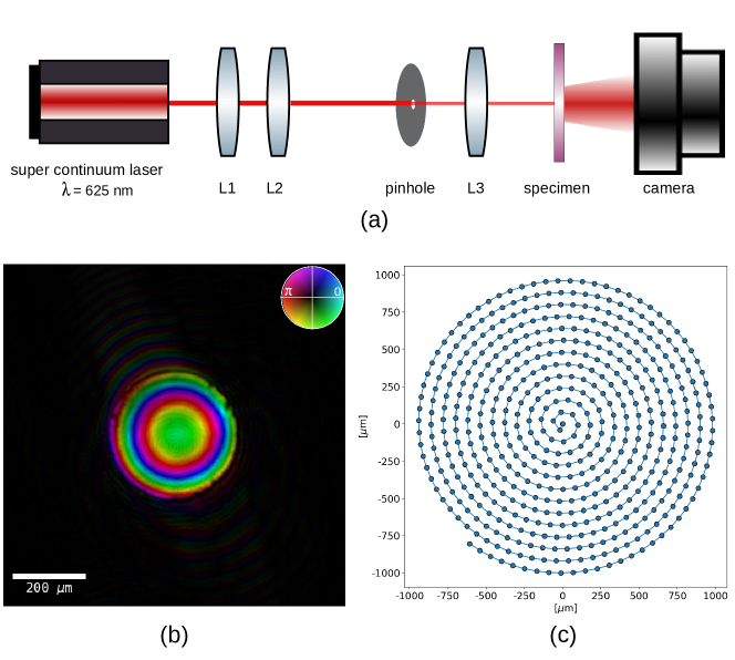
Figure 6: (a) Experimental ptychography setup in transmission geometry. (b) Probe beam of size $400\,\mu m$ characterized with ptychographic reconstruction. (c) Concentric scanning grid used in the experiment.

In this experiment, we use the unstained histological mouse section as our object. The ptychography experiment is designed by deciding the object-detector distance to be $23.7\,mm$ and a binning of factor $8$ that effectively reduces the resolution to $684\times 456$. The probe field of view (FOV) can then be calculated to be $\approx 771.4\,\mu m$. Based on the theoretical consideration for the probe to be approximately half of the probe field of view, a pinhole of size $400\,\mu m$ ensures that (see Fig. 6 (b)). We select $500$ scan positions for a concentric spiral scan grid with the radius of $1.009\,mm$ as shown in figure 6 (c) and the probe overlap between adjacent scan positions is $80\,\%$. Therefore, we can reconstruct an area of $\approx 3.2\,mm^{2}$ from our mouse specimen.

References

- Baksh et al. (2016) Baksh, P. D., Odstrčil, M., Kim, H.-S., Boden, S. A., Frey, J. G., and Brocklesby, W. S. Wide-field broadband extreme ultraviolet transmission ptychography using a high-harmonic source. Opt. Lett., 41(7):1317–1320, Apr 2016.
- Dempster et al. (1977) Dempster, A. P., Laird, N. M., and Rubin, D. B. Maximum likelihood from incomplete data via the em algorithm. Journal of the Royal Statistical Society: Series B (Methodological), 39(1):1–22, 1977.
- Dierolf et al. (2010) Dierolf, M., Thibault, P., Menzel, A., Kewish, C. M., Jefimovs, K., Schlichting, I., von König, K., Bunk, O., and Pfeiffer, F. Ptychographic coherent diffractive imaging of weakly scattering specimens. New Journal of Physics, 12(3):035017, Mar 2010.
- Eschen et al. (2024) Eschen, W., Liu, C., Steinert, M., Molina, D. S. P., Siefke, T., Zeitner, U. D., Kaspar, J., Pertsch, T., Limpert, J., and Rothhardt, J. Structured illumination ptychography and at-wavelength characterization with an euv diffuser at 13.5 nm wavelength. Opt. Express, 32(3):3480–3491, Jan 2024.
- Gelman et al. (2013) Gelman, A., Carlin, J. B., Stern, H. S., Dunson, D. B., Vehtari, A., and Rubin, D. B. Bayesian Data Analysis. Chapman and Hall/CRC, November 2013.
- Kandel et al. (2019) Kandel, S., Maddali, S., Allain, M., Hruszkewycz, S. O., Jacobsen, C., and Nashed, Y. S. G. Using automatic differentiation as a general framework for ptychographic reconstruction. Opt. Express, 27(13):18653–18672, Jun 2019.
- Kodgirwar et al. (2024) Kodgirwar, S., Loetgering, L., Liu, C., Joseph, A., Licht, L., Molina, D. S. P., Eschen, W., Rothhardt, J., and Habeck, M. Supplementary software and data: Bayesian multi-exposure image fusion for robust high dynamic range preprocessing in ptychography, March 2024.
- Liu et al. (2023) Liu, J., Liu, C., Zou, C., Zhao, Y., and Liu, J. Large dynamic range dark-field imaging based on microscopic images fusion. Optics Communications, 528:128966, 2023. ISSN 0030-4018.
- Lo et al. (2018) Lo, Y. H., Zhao, L., Gallagher-Jones, M., Rana, A., J. Lodico, J., Xiao, W., Regan, B. C., and Miao, J. In situ coherent diffractive imaging. Nature Communications, 9(1):1826, May 2018. ISSN 2041-1723.
- Loetgering et al. (2022) Loetgering, L., Witte, S., and Rothhardt, J. Advances in laboratory-scale ptychography using high harmonic sources [invited]. Opt. Express, 30(3):4133–4164, Jan 2022.
- Loetgering et al. (2023) Loetgering, L., Du, M., Flaes, D. B., Aidukas, T., Wechsler, F., Molina, D. S. P., Rose, M., Pelekanidis, A., Eschen, W., Hess, J., Wilhein, T., Heintzmann, R., Rothhardt, J., and Witte, S. Ptylab.m/py/jl: a cross-platform, open-source inverse modeling toolbox for conventional and fourier ptychography. Opt. Express, 31(9):13763–13797, Apr 2023.
- Maiden et al. (2017) Maiden, A., Johnson, D., and Li, P. Further improvements to the ptychographical iterative engine. Optica, 4(7):736–745, Jul 2017.
- Maiden & Rodenburg (2009) Maiden, A. M. and Rodenburg, J. M. An improved ptychographical phase retrieval algorithm for diffractive imaging. Ultramicroscopy, 109(10):1256–1262, 2009. ISSN 0304-3991.
- Odstrcil et al. (2016) Odstrcil, M., Baksh, P., Boden, S. A., Card, R., Chad, J. E., Frey, J. G., and Brocklesby, W. S. Ptychographic coherent diffractive imaging with orthogonal probe relaxation. Opt. Express, 24(8):8360–8369, Apr 2016.
- Odstrčil et al. (2019) Odstrčil, M., Lebugle, M., Guizar-Sicairos, M., David, C., and Holler, M. Towards optimized illumination for high-resolution ptychography. Opt. Express, 27(10):14981–14997, May 2019.
- Plackett (1953) Plackett, R. L. The truncated poisson distribution. Biometrics, 9(4):485, December 1953.
- Rodenburg & Maiden (2019) Rodenburg, J. and Maiden, A. Ptychography, pp. 819–904. Springer International Publishing, Cham, 2019. ISBN 978-3-030-00069-1.
- Rose et al. (2018) Rose, M., Senkbeil, T., von Gundlach, A. R., Stuhr, S., Rumancev, C., Dzhigaev, D., Besedin, I., Skopintsev, P., Loetgering, L., Viefhaus, J., Rosenhahn, A., and Vartanyants, I. A. Quantitative ptychographic bio-imaging in the water window. Opt. Express, 26(2):1237–1254, Jan 2018.
- Seifert et al. (2023) Seifert, J., Shao, Y., van Dam, R., Bouchet, D., van Leeuwen, T., and Mosk, A. P. Maximum-likelihood estimation in ptychography in the presence of poisson–gaussian noise statistics. Opt. Lett., 48(22):6027–6030, Nov 2023.
- Shafie et al. (2009) Shafie, S., Kawahito, S., Halin, I. A., and Hasan, W. Z. W. Non-linearity in wide dynamic range CMOS image sensors utilizing a partial charge transfer technique. Sensors (Basel), 9(12):9452–9467, Nov 2009.
- Singh et al. (2022) Singh, H., Cristobal, G., Bueno, G., Blanco, S., Singh, S., Hrisheekesha, P., and Mittal, N. Multi-exposure microscopic image fusion-based detail enhancement algorithm. Ultramicroscopy, 236:113499, 2022. ISSN 0304-3991.
- Thibault & Guizar-Sicairos (2012) Thibault, P. and Guizar-Sicairos, M. Maximum-likelihood refinement for coherent diffractive imaging. New Journal of Physics, 14(6):063004, Jun 2012.
- Thibault et al. (2008) Thibault, P., Dierolf, M., Menzel, A., Bunk, O., David, C., and Pfeiffer, F. High-resolution scanning x-ray diffraction microscopy. Science, 321(5887):379–382, 2008.
- Van der Walt et al. (2014) Van der Walt, S., Schönberger, J. L., Nunez-Iglesias, J., Boulogne, F., Warner, J. D., Yager, N., Gouillart, E., and Yu, T. scikit-image: image processing in python. PeerJ, 2:e453, 2014.
- Wang et al. (2004) Wang, Z., Bovik, A., Sheikh, H., and Simoncelli, E. Image quality assessment: from error visibility to structural similarity. IEEE Transactions on Image Processing, 13(4):600–612, 2004.
- Xu et al. (2022) Xu, F., Liu, J., Song, Y., Sun, H., and Wang, X. Multi-exposure image fusion techniques: A comprehensive review. Remote Sensing, 14(3), 2022. ISSN 2072-4292.
- Yin et al. (2015) Yin, Z., Su, H., Ker, E., Li, M., and Li, H. Cell-sensitive phase contrast microscopy imaging by multiple exposures. Medical Image Analysis, 25(1):111–121, 2015. ISSN 1361-8415.
- Zhang et al. (2016) Zhang, F., Chen, B., Morrison, G. R., Vila-Comamala, J., Guizar-Sicairos, M., and Robinson, I. K. Phase retrieval by coherent modulation imaging. Nature Communications, 7(1):13367, Nov 2016. ISSN 2041-1723.
- Zhang (2021) Zhang, X. Benchmarking and comparing multi-exposure image fusion algorithms. Information Fusion, 74:111–131, 2021. ISSN 1566-2535.