Federated Transfer Learning with Differential Privacy

Abstract

Federated learning is gaining increasing popularity, with data heterogeneity and privacy being two prominent challenges. In this paper, we address both issues within a federated transfer learning framework, aiming to enhance learning on a target data set by leveraging information from multiple heterogeneous source data sets while adhering to privacy constraints. We rigorously formulate the notion of federated differential privacy, which offers privacy guarantees for each data set without assuming a trusted central server. Under this privacy constraint, we study three classical statistical problems, namely univariate mean estimation, low-dimensional linear regression, and high-dimensional linear regression. By investigating the minimax rates and identifying the costs of privacy for these problems, we show that federated differential privacy is an intermediate privacy model between the well-established local and central models of differential privacy. Our analyses incorporate data heterogeneity and privacy, highlighting the fundamental costs of both in federated learning and underscoring the benefit of knowledge transfer across data sets.

1 Introduction

As data availability burgeons, research on data aggregation is gaining growing prominence, offering possible improvements in learning a target data set by gathering useful information from related sources. This however also resulted in concerns on data privacy and stimulated research on federated learning (e.g. Konečnỳ et al., 2016; McMahan et al., 2017; Li et al., 2020a). In federated learning, the exchange of summary statistics, such as gradients and Hessian matrices, facilitates the aggregation of information without transferring raw data among different sites. Despite these advancements, recent studies have revealed potential privacy vulnerabilities, even with the communication of gradients and Hessian matrices (Wang et al., 2019). In some instances, attackers can reconstruct original images at the pixel level in image data sets (Zhu et al., 2019; Zhao et al., 2020), underscoring the need for a more robust privacy protection mechanism.

In response to the demand for protecting data privacy, differential privacy (DP) emerges as a widely adopted notion (Dwork et al., 2006, 2014). Recent works have connected DP with federated learning to address the privacy challenges highlighted above (e.g. Geyer et al., 2017; Dubey and Pentland, 2020; Lowy and Razaviyayn, 2021; Liu et al., 2022; Allouah et al., 2023; Zhou and Chowdhury, 2023), mainly focusing on empirical risk minimisation and usually aiming to minimise an ‘average risk’ defined over all participating data sets. Such emphasises have solid practical implications, whereas in the context of transfer learning (TL), one is mostly concerned about learning in a target data set, with the presence of similar and/or dissimilar source data sets. Blindly applying existing federated learning techniques without accounting for the potential presence of disparate sources, could damage the learning performance on the target data set. This is known as the ‘negative transfer’ phenomenon in the TL literature (e.g. Rosenstein et al., 2005; Yao and Doretto, 2010; Hanneke and Kpotufe, 2019).

Identifying the gaps in the TL literature that pertain to rigorous privacy guarantees, we, in this paper, formalise the notion of federated transfer learning (FTL) within a novel DP framework. The general problem setup and the privacy framework are introduced in the rest of Section 1. Under this framework, we investigate the impact of privacy constraints and source data heterogeneity on statistical estimation error rates. In particular, we study three classical statistical problems with increasing dimensionality, from univariate mean estimation in Section 2, to low-dimensional linear regression in Section 3, and finally high-dimensional linear regression in Section 4. For the first two problems, we establish matching upper and lower bounds (up to logarithmic factors) on the minimax rates to quantify the costs of data heterogeneity and privacy. For the last problem, which lies in largely uncharted territory in the FTL context, we propose an algorithm with an upper bound on the estimation error and discuss its optimality. We conclude with a discussion section (Section 5) on potential future directions and defer all the proofs and technical details to the Appendices.

1.1 Federated transfer learning

Throughout this paper, we work under an FTL framework, where the goal is to improve the learning performance on a target data set collected from one site by effectively including auxiliary source data sets collected from other sites, while protecting the privacy of each individual data set. To be specific, let $D_{0}$ be the target data set, $\{D_{k}\}_{k\in[K]}$ be the $K$ source data sets, where $K\in\mathbb{Z}_{+}$ and $[K]=\{1,\ldots,K\}$, and $\mathcal{P}$ be a family of distributions. For $k\in\{0\}\cup[K]$, assume observations in $D_{k}$ are independent and identically distributed with distribution $P_{\theta^{(k)}}\in\mathcal{P}$, where $\theta^{(k)}\in\mathbb{R}^{d}$ is the parameter of interest.

An inherent challenge in the multi-source setting is to identify useful source data sets in order to learn a better model for the target data, and the degree of ‘similarity’ between target and source data sets typically determines the utility of the source data. In parametric settings, it is natural to measure the similarity between the target and the $k$-th source through $\rho(\theta^{(0)},\theta^{(k)})$, where $\rho$ is some metric in $\mathbb{R}^{d}$. In this work, we consider the $\ell_{2}$-distance $\rho(\theta^{(0)},\theta^{(k)})=\|\theta^{(0)}-\theta^{(k)}\|_{2}$ and assume $\max_{k\in\mathcal{A}}\|\theta^{(0)}-\theta^{(k)}\|_{2}\leq h$, where $\mathcal{A}\subseteq[K]$ and $h\geq 0$ are both unknown. The quantity $h$ measures the similarity level, with lower values of $h$ indicating a higher level of similarity between the sources within the index set $\mathcal{A}$ and the target.

Our aim is to estimate $\theta^{(0)}$ by leveraging all the information in the data $\{D_{k}\}_{k\in\{0\}\cup[K]}$, with the hope to improve the target-only estimator, i.e. estimators only using the target data $D_{0}$. Intuitively, we hope to combine those source data sets that are sufficiently similar to the target data set. As motivated before, however, directly combining information from separate data sets can incur serious privacy concerns. Throughout this paper, we, therefore, study FTL procedures that are subject to a novel DP constraint (see Section 1.2), which offers privacy guarantees to each data set without relying on any trusted central server to combine the information.

1.2 Privacy framework

The prevailing framework for developing private methodology is differential privacy (DP, Dwork et al., 2006). The most standard definition of DP considers a centralised setting, where there exists a trusted data curator that has access to everyone’s raw data. Given a data set $D$ with sample size $n$, a privacy mechanism $Q(\cdot|D)$ is a conditional distribution of the private information given the data. Let $Z\in\mathcal{Z}$ denote the private information. For $\epsilon>0$ and $\delta\geq 0$, the privacy mechanism $Q$ is said to satisfy $(\epsilon,\delta)$-central DP, if for all possible $D$ and $D^{\prime}$ that differ by at most one data entry, it holds that

$$Q(Z\in S|D)\leq e^{\epsilon}Q(Z\in S|D^{\prime})+\delta,$$ (1)

for all measurable sets $S\subseteq\mathcal{Z}$. The parameter $\epsilon$ measures the strength of privacy guarantees – the smaller $\epsilon$, the stronger the constraint. A typical regime of interest is when $\epsilon\in(0,1)$. The parameter $\delta\in[0,1)$ can be understood as the probability of privacy leakage, and it is usually required that $\delta$ be much smaller than $1/n$ to obtain a satisfactory formulation of privacy.

As can be seen from (1), in the central setting, the privacy mechanism $Q$ can use information in the entire data set comprising many individuals from potentially different locations. Allowing the central server to have access to all the raw data poses a significant privacy threat in the federated setting. It can also be unrealistic in practice. For example, patients may trust their hospital to handle their sensitive information in exchange for more personalised and effective treatments. However, they may not want such information to be leaked to any third party.

Motivated by such restrictions, we consider a form of privacy constraints, namely federated differential privacy (FDP). Our constraint requires that each site protects its information locally and only communicates the privatised information to the central server for analysis.

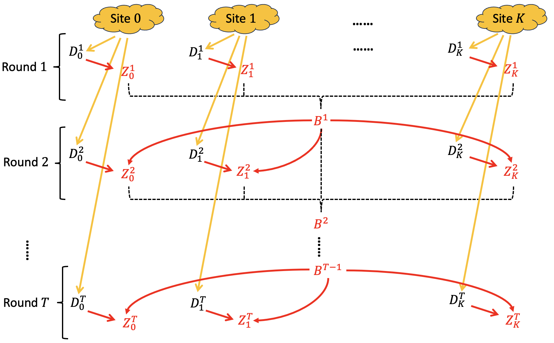
Figure 1: An illustration of the privacy mechanisms that satisfy 1. For $t\in[T]$ and $k\in\{0\}\cup[K]$, $D_{k}^{t}$ and $Z_{k}^{t}$ refer to the data used in round $t$ at site $k$ and the communicated private information in round $t$ from site $k$, respectively; $B^{t}=(\{Z_{k}^{t}\}_{k\in\{0\}\cup[K]},B^{t-1})$ is the set of private information from all $K+1$ sites in and before round $t$. Privacy mechanisms are applied to obtain each $Z_{k}^{t}$ using the information in $D_{k}^{t}$ and $B^{t-1}$.

Recall that in the FTL setting, we have $K+1$ data sets $\{D_{k}\}_{k\in\{0\}\cup[K]}$. We consider a $T$-round interaction scheme, as shown in Figure 1. In the $t$-th round of communication, $t\in[T]$, private information $Z_{k}^{t}$ is produced using some privacy mechanism $Q_{k}^{t}$ at each site $k\in\{0\}\cup[K]$. Let $\{D_{k}^{t}\}_{t\in[T]}$ form a partition of $D_{k}$, i.e. $D_{k}=\cup_{t=1}^{T}D_{k}^{t}$ with mutually disjoint and non-empty $\{D_{k}^{t}\}_{t\in[T]}$. We write $B^{t}=(\{Z^{t}_{k}\}_{k\in\{0\}\cup[K]},B^{t-1})$ to denote all information communicated across different sites in and before round $t$, and set $B^{0}=1$.

To generate $Z_{k}^{t}$, as shown in Figure 1, the privacy mechanism $Q_{k}^{t}(\cdot|D_{k}^{t},B^{t-1})$ can use the information contained in a subset of the whole data at site $k$ and the private information $B^{t-1}$ accumulated from previous rounds. The privacy mechanisms are required to satisfy the following FDP constraint.

Definition 1 (Federated Differential Privacy, FDP).

Let $Q=\{Q_{k}^{t}\}_{k\in\{0\}\cup[K],t\in[T]}$ denote the collection of all the privacy mechanisms across sites and iterations. For $\epsilon>0$, $\delta\geq 0$ and $T,K\in\mathbb{Z}_{+}$, we say $Q$ is FDP with parameter $(\epsilon,\delta)$, denoted as $(\epsilon,\delta)$-FDP, if for all $t\in[T]$, $k\in\{0\}\cup[K]$, it holds that

$$Q_{k}^{t}(Z_{k}^{t}\in S|D_{k}^{t},B^{t-1})\leq e^{\epsilon}Q_{k}^{t}(Z_{k}^{t}\in S|(D_{k}^{t})^{\prime},B^{t-1})+\delta,$$ (2)

for any measurable set $S$, and all possible $D_{k}^{t}$ and $(D_{k}^{t})^{\prime}$ that differ in at most one data entry, with $Z_{k}^{t}$, $D_{k}^{t}$ and $B^{t-1}$ defined above.

Remark 1.

Given the parameters $\epsilon,\delta$ and $T$, we denote the class of privacy mechanisms satisfying 1 as $\mathcal{Q}_{\epsilon,\delta,T}$. The parameters $\epsilon$ and $\delta$ have the same interpretations as those in the central DP setting. The choice of $T$ needs to ensure that $\{D_{k}^{t}\}_{t\in[T]}$ form a partition of $D_{k}$, for each $k$, and its value cannot exceed the smallest sample size among $\{D_{k}\}_{k\in\{0\}\cup[K]}$. Writing $Z=\{Z_{k}^{t}\}_{k\in\{0\}\cup[K],t\in[T]}$ as the entire private communication transcript, we also say an algorithm is $(\epsilon,\delta)$-FDP, if it only depends on $Z$.

Remark 2.

We note that similar notions of privacy have been considered in a range of recent studies (e.g. Allouah et al., 2023; Lowy and Razaviyayn, 2021; Zhou and Chowdhury, 2023; Liu et al., 2022) under different names and formulations; see Section 1.5 for more in-depth discussions. We emphasise that most of the existing literature with similar privacy guarantees considers learning a single model for data across all sites, whereas our study focuses on the transfer learning perspective.

In the special case of $T=1$, the condition in (2) essentially reduces to

$$Q_{k}(Z_{k}\in S|D_{k})\leq e^{\epsilon}Q_{k}(Z_{k}\in S|(D_{k})^{\prime})+\delta,$$ (3)

for all possible $D_{k}$ and $(D_{k})^{\prime}$ that differ in at most one data entry, where $Z_{k}\in\mathcal{Z}_{k}$ is produced by a privacy mechanism $Q_{k}$ from each site $k\in\{0\}\cup[K]$, without using any information from other sites. In this case, we say $Q=\{Q_{k}\}_{\{0\}\cup[K]}$ satisfy non-interactive FDP with parameters $(\epsilon,\delta)$ and denote the corresponding class of privacy mechanisms as $\mathcal{Q}_{\epsilon,\delta,1}$. The advantage of non-interactive mechanisms is that they do not incur any communication costs inter-sites when producing private information. The restriction of non-interactivity, however, excludes interactive privacy mechanisms that could be potentially more efficient in complicated problems. We consider non-interactive FDP mechanisms for univariate mean estimation problems in Section 2 and general FDP mechanisms (1) for linear regression problems in Sections 3 and 4.

Note that the FDP notion guarantees privacy for each site at the ‘item-level’, which is similar to the guarantee offered by the usual central DP definition in (1). In particular, FDP implies a central DP type guarantee for each site separately, as discussed in Section 1.5. In the special case when $n_{k}=1$ for all $k\in\{0\}\cup[K]$, (3) coincides with the definition of non-interactive local differential privacy (LDP) (e.g. Duchi et al., 2018); see the corresponding definition and discussion in Section 1.5. In fact, an appealing feature of the FDP framework is that it provides an intermediate privacy model between the well-studied central and local models of DP; see our discussions and comparisons in Sections 1.4, 2.3, 3.3 and 4.3.

1.3 Minimax risk under FDP constraints

To investigate the impact of privacy constraints and source heterogeneity on learning the target model, we adopt the minimax framework. Consider the parameter space

$$\Theta(\mathcal{A},h)=\left\{\bm{\theta}=\{\theta^{(k)}\}_{k\in\{0\}\cup[K]}:\max_{k\in\mathcal{A}}\rho(\theta^{(k)},\theta^{(0)})\leq h\right\},$$ (4)

specified by $\mathcal{A}\subseteq[K]$ and $h\geq 0$. The source data sets in $\mathcal{A}$ are assumed to be similar to the target data set with the difference measured by some metric $\rho$ upper bounded by $h$. Sources that are potentially very different from the target are collected in $\mathcal{A}^{c}$. We note that although $\mathcal{A}$ and $h$ are required to specify the parameter space in (4), which is crucial for defining the minimax risk, our algorithms do not require such knowledge. We develop a general detection strategy, as described in Appendix A, automatically selecting a set $\hat{\mathcal{A}}\subseteq[K]$ without using any information about $\mathcal{A}$ and $h$. We then apply appropriately privatised federated learning algorithms onto this selected informative set $\hat{\mathcal{A}}$ and show that they can lead to nearly optimal performance.

We consider the minimax risk under FDP constraints, defined as

$$\inf_{\begin{subarray}{c}Q\in\mathcal{Q}_{\epsilon,\delta,T}\end{subarray}}\inf_{\hat{{\theta}}(Z)}\sup_{P_{\bm{\theta}}\in\mathcal{P}(\Theta(\mathcal{A},\,h))}\mathbb{E}_{P_{\bm{\theta}},Q}\{\rho(\hat{{\theta}}(Z),{\theta}^{(0)})\},$$

where $\mathcal{P}(\Theta(\mathcal{A},h))$ denotes the class of joint distributions of all data from the target and source data sets with $P_{{\theta}^{(k)}}\in\mathcal{P}$ for all $k\in\{0\}\cup[K]$ and $\bm{\theta}=\{\theta^{(k)}\}_{k\in\{0\}\cup[K]}\in\Theta(\mathcal{A},h)$. The estimator $\hat{\theta}(Z)$ is a measurable function of the privatised information $Z$, the entire private communication transcript, generated from some privacy mechanism $Q\in\mathcal{Q}_{\epsilon,\delta,T}$.

1.4 Contributions

In this paper, we study three specific problems under the FTL setup, where the goal is to improve learning on the target data set by utilising information from multiple source data sets with potentially heterogeneous data generating mechanisms. To provide rigorous privacy guarantees that are suitable for such settings, we formulate FDP (1), which offers site-specific privacy guarantees without a trusted central server. We investigate the minimax risk for different problems under such privacy constraints.

We consider three classical statistics problems with increasing dimensionality. For the univariate mean estimation problem (Section 2) and the low-dimensional linear regression problem (Section 3), where the covariate dimension $d$ is assumed to be smaller than the sample size at each site, we develop private federated learning procedures and establish their optimality when the target and all source data sets have balanced sample sizes. In particular, the minimax rates take the form of

$$\text{Target-only Rate}\,\,\wedge\,\,{\text{FDP Rate}},$$

where the target-only rate corresponds to learning only using the target data subject to central DP constraints, and the FDP rate arises when combining information across source data sets subject to FDP constraints.

Specific rates for all three problems are presented in Table 1. Note that for the high-dimensional regression problem (Section 4), we only obtain an upper bound on the corresponding FDP rate and we provide a discussion on its connection to the setting under LDP constraint and the conjecture on its tightness in Section 4.3.

Problems	Target-only	FDP
Univariate mean estimation	$\frac{1}{\sqrt{n}}+\frac{1}{n\epsilon}$	$h+\sqrt{\frac{1}{{|\mathcal{A}|n}}}+\frac{1}{n\epsilon\sqrt{|\mathcal{A}|}}$
Low-dimensional regression	$\sqrt{\frac{d}{n}}+\frac{d}{n\epsilon}$	$h+\sqrt{\frac{d}{|\mathcal{A}|n}}+\frac{d}{n\epsilon\sqrt{|\mathcal{A}|}}$
High-dimensional regression	$\sqrt{\frac{s}{n}}+\frac{s}{n\epsilon}$	$h+\sqrt{\frac{s}{|\mathcal{A}|n}}+\frac{\sqrt{sd}}{n\epsilon\sqrt{|\mathcal{A}|}}$

Table 1: A summary of our main results. For clarity, we assume $\mathcal{A}\neq\emptyset$. The parameter $n$ is the number of observations at the target and each source data set, $h$ measures the heterogeneity between the source data sets in $\mathcal{A}$ and the target data set, $d$ is the dimension of the covariates in regression problems, $s$ is the sparsity level in the high-dimensional regression problem, and $\epsilon$ is the privacy parameter.

Comparing FDP rates with target-only rates, our results quantify the costs and benefits of private FTL with heterogeneous source data sets. Note that target-only rates consist of two parts - non-private and private rates, while FDP rates involve three - non-private, private and heterogeneity ($h$) rates. When $h$ is small and $|\mathcal{A}|$ is large, i.e. there are sufficient informative source data sets for learning the target parameter, FDP rates offer improvement compared to target-only ones.

An interesting phenomenon is that, in FDP rates, $|\mathcal{A}|$ contributes non-private and private parts differently. Since we assume $\mathcal{A}\neq\emptyset$, non-private terms depend on $n|\mathcal{A}|\asymp n(|\mathcal{A}|+1)$ - the total sample size of the target and source data sets in $\mathcal{A}$. However, in private terms, the relationship between $n$ and $|\mathcal{A}|$ becomes $n\sqrt{|\mathcal{A}|}$. This phenomenon is unique to the FDP constraint and it has been recently observed in the context of federated empirical risk minimisation under similar privacy definitions (Lowy and Razaviyayn, 2021; Allouah et al., 2023). We also compare our results with results under central DP and LDP privacy constraints for these problems in Sections 2.3, 3.3 and 4.3. These comparisons demonstrate that FDP is an intermediate model between these two well-known models of DP, and FDP rates interpolate the corresponding results.

On the technical side, our contributions include the following.

• We develop a general detection procedure to identify the informative source data sets, as described in Appendix A. This procedure compares private estimates on each source data set to the private estimate on the target data set, and uses the accuracy of the target estimate as a threshold for selection. We show that our detection procedure can recover $\mathcal{A}$ with high probability, when the distributions for sites in $\mathcal{A}^{c}$ are sufficiently different from that of the target data set, and the final estimator never performs worse than using the target data alone.

• For the regression problems that we consider in Sections 3 and 4, we use the recently proposed adaptive clipping strategy (Varshney et al., 2022) to achieve optimality over a larger range of parameters compared to Cai et al. (2019). Although this methodology has been used for analysing low-dimensional linear regression problems in a single site under central DP constraints (Varshney et al., 2022; Liu et al., 2023), we simplify previous analyses and generalise it to federated and high-dimensional settings.

• We establish minimax lower bounds under the FDP constraints for the mean estimation and low-dimensional linear regression problems in Sections 2.3 and 3.3, respectively. For the mean estimation problem, our lower bound proof naturally combines techniques in the central DP and LDP literature, which reflects the fact that the FDP setup is a mixture of these two well-studied privacy models. For the linear regression problem, we adapt a privacy amplification result in Lowy and Razaviyayn (2021), which transforms an FDP problem into a central DP problem, to deal with the presence of disparate sources in our setting.

1.5 Related work

In view of the nature of the FDP constraints we consider in this paper, in this section, we briefly review three related areas: federated learning, transfer learning and differential privacy.

Federated learning is introduced as a privacy-preserving solution for user information sharing in decentralised and distributed settings, where the direct communication of raw data among different data sets is prohibited. A typical problem in the federated setting concerns learning a shared model or minimising an averaged risk across all sites/users (e.g. Konečnỳ et al., 2016; McMahan et al., 2017; Li et al., 2020b). When there is significant heterogeneity across different sites, learning a single shared model becomes an ill-posed problem, and therefore another line of work focuses on multi-task or personalised federated learning (e.g. Smith et al., 2017; Li et al., 2020b; T Dinh et al., 2020; Chen et al., 2021; Marfoq et al., 2021; Chen et al., 2023; Li et al., 2023a), where the goal is to learn a model for each site while utilising potentially useful auxiliary information from other sites.

Transfer learning (TL) shares similar spirits with multi-task learning, but focuses on improving learning of a single target data set by strategically aggregating information from multiple source data sets. Many works on TL consider empirical risk minimisation (e.g. Ando et al., 2005; Evgeniou et al., 2005; Maurer, 2006; Ben-David et al., 2010; Hanneke and Kpotufe, 2019; Tripuraneni et al., 2020; Cai and Wei, 2021; Du et al., 2021; Reeve et al., 2021). There is also a growing body of research focusing on statistical estimation and inference, especially in the supervised learning setting (e.g. Bastani, 2021; Liu et al., 2021; Li et al., 2022; Lin and Reimherr, 2022; Maity et al., 2022; Tian and Feng, 2023a; Tian et al., 2022; Zhou et al., 2022; Duan and Wang, 2023; Li et al., 2023c, b), where three categories emerge based on the distributional differences of $X$ and $Y|X$ between the target and source data sets. These categories include covariate shift - distinct distributions of $X$ with identical distributions of $Y|X$, posterior drift - distinct distributions of $Y|X$ with identical distributions of $X$, and concept drift - difference in distributions of both $X$ and $Y|X$ (Pan and Yang, 2009). Our study of regression problems in this paper falls into the category of concept drift as we allow heterogeneity between both $X$ and $Y|X$ distributions across target and source data sets.

Differential privacy techniques have been increasingly used in federated and distributed learning settings in recent years. Most of the existing literature, however, focuses on providing a central DP type guarantee, either at the item-level or user-level (e.g. Geyer et al., 2017; McMahan et al., 2017; Ghazi et al., 2021; Levy et al., 2021; Jain et al., 2021), requiring a trusted central server to coordinate and collect information from different sites. Techniques from multi-party computation (e.g. Jayaraman et al., 2018; Agarwal et al., 2021; Chen et al., 2022; Heikkilä et al., 2020; Kairouz et al., 2021), and adding a trusted shuffler between users and the central server (e.g. Erlingsson et al., 2019; Cheu et al., 2019; Cheu, 2021; Feldman et al., 2022) have been proposed to offer central DP guarantee while limiting the information directly accessed by the central server, but their claimed utility results and privacy guarantee still rely on some trust across different sites and/or on the server side; see also the discussion in Liu et al. (2022). On the contrary, in the FDP framework, all the information communicated among different sites and the central server is privatised. Privacy at each site is therefore protected against any inference attack from potential untrusted servers or adversarial sites; see Figure 2 for a schematic illustration.

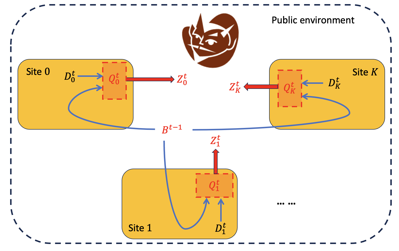
Figure 2: FDP provides a privacy guarantee for each site without relying on any trusted third party.

FDP can be viewed as offering a central DP type guarantee for each site separately. Recall the setup in Section 1.2, where $Z=\{Z_{k}^{t}\}_{k\in\{0\}\cup[K],t\in[T]}$ denotes the entire private communication transcript. We further write $Z_{k}=\{Z_{k}^{t}\}_{t\in[T]}$ and $Z_{\setminus k}=Z\setminus Z_{k}$, $k\in\{0\}\cup[K]$. Applying parallel composition (e.g. Smith et al., 2021) to $Q_{k}^{t}$ satisfying (2) then implies that

$$\mathbb{P}(Z_{k}\in S|D_{k},Z_{\setminus k}=z_{\setminus k})\leq\exp(\epsilon)\mathbb{P}(Z_{k}\in S|(D_{k})^{\prime},Z_{\setminus k}=z_{\setminus k})+\delta,$$ (5)

for any measurable set $S$ and any pair $D_{k}$, $(D_{k})^{\prime}$ that differ by at most one entry. This type of guarantee in (5) - slightly weaker than the FDP constraint in (2), has appeared bearing different names in the literature, including inter-silo record-level DP in Lowy and Razaviyayn (2021, Definition 5), silo-level LDP in Zhou and Chowdhury (2023, Defniition 3.1), silo-specific sample-level DP in Liu et al. (2022, Definition 3.1), and $(\epsilon,\delta)$-distributed DP in Allouah et al. (2023, Definition 2.3) among others. In these works, minimax lower bounds are derived in Lowy and Razaviyayn (2021) and Allouah et al. (2023). In order to establish the lower bounds, Lowy and Razaviyayn (2021), instead of considering (5), also restricts to a form of privacy guarantee that is similar to our 1, but without sample splitting in each iteration. In Allouah et al. (2023), the lower bounds are established under the larger class of privacy mechanisms (5), but their arguments treat the data as fixed.

One of the appealing features of FDP is that it provides an intermediate privacy model between central DP and LDP; see the discussion in Section 1.4 and comparisons in Sections 2.3, 3.3 and 4.3. With central DP and FDP introduced in (1) and (2), we now turn to the concept of LDP. LDP is the strongest notion of privacy among these three. Each user submits a privatised version of their data to the central server without passing through the site administrator. Formally, suppose that each user $u\in[U]$, $U\in\mathbb{Z}_{+}$, holds data $X_{u}\in\mathcal{X}$ and generates private data $Z_{u}\in\mathcal{Z}$ using some privacy mechanism $Q_{u}$. The private information $Z_{u}$ is said to be an $\epsilon$-LDP view of $X_{u}$, if for all $x_{u},x_{u}^{\prime}\in\mathcal{X}$, it holds that

$$Q_{u}(Z_{u}\in S|x_{u})\leq\exp(\epsilon)Q_{u}(Z_{u}\in S|x_{u}^{\prime}),$$ (6)

for any measurable set $S$. The version presented in (6) is arguably the simplest design of LDP schemes, known as non-interactive LDP mechanisms (Duchi et al., 2018). This also coincides with the notion of non-interactive FDP (3) when $n_{k}=1$ for all $k\in\{0\}\cup[K]$. More general designs of mechanisms that allow some form of interaction among the users have been considered in the literature (e.g. Duchi et al., 2018; Duchi and Rogers, 2019; Joseph et al., 2019; Acharya et al., 2020).

When comparing with LDP settings in our paper, we focus on the pure $\epsilon$-LDP instead of the approximate $(\epsilon,\delta)$-LDP since several existing works have shown that moving from pure to approximate in the LDP setting does not yield more accurate algorithms (e.g. Bassily and Smith, 2015; Bun et al., 2019; Duchi and Rogers, 2019).

1.6 Notation

For a set $S$, we use $|S|$ to denote its cardinality. A random variable $X$ has standard Laplace distribution if it has density $f(x)=\exp(-|x|)/2$. For a matrix $\bm{A}$, we use $\lambda_{\min}(\bm{A})$ and $\lambda_{\max}(\bm{A})$ to denote the smallest and largest eigenvalues of $\bm{A}$, respectively. If $\bm{A}$ is a symmetric square matrix, $\bm{A}\succ 0$ means it is positive definite, and $\|\bm{A}\|_{2}=\lambda_{\max}(\bm{A})$ represents its operator norm. For a vector ${x}=(x_{1},\ldots,x_{d})\in\mathbb{R}^{d}$, we define its $\ell_{0}$-pseudo-norm, $\ell_{2}$- and $\ell_{\infty}$-norms as $\|x\|_{0}=|\{j\in[d]:x_{j}\neq 0\}|$, $\|x\|_{2}=\sqrt{\sum_{j=1}^{d}x_{j}^{2}}$ and $\|x\|_{\infty}=\max_{j\in[d]}|x_{j}|$, respectively. With $R>0$, we write $\Pi_{R}(x)=x\min\{1,R/\|x\|_{2}\}$ as the projection of vector $x\in\mathbb{R}^{d}\setminus\{0\}$ onto the $\ell_{2}$-ball in $\mathbb{R}^{d}$ of radius $R$ and centred at the origin. We use $\prod_{R}^{\infty}(x)=x\min\{1,R/\|x\|_{\infty}\}$ to denote the projection of $x\in\mathbb{R}^{d}\setminus\{0\}$ onto the $\ell_{\infty}$-ball in $\mathbb{R}^{d}$ of radius $R$ and centred at the origin. For two real positive series $\{a_{n}\}_{n=1}^{\infty}$ and $\{b_{n}\}_{n=1}^{\infty}$, we write $a_{n}\lesssim b_{n}$ or $a_{n}=\mathcal{O}(b_{n})$ when there exists absolute constants $C>0$ and $N_{0}\in\mathbb{Z}_{+}$ such that $a_{n}\leq Cb_{n}$ for all $n\geq N_{0}$, and we write $a_{n}\gtrsim b_{n}$ or $a_{n}=\Omega(b_{n})$ when there exists absolute constants $C>0$ and $N_{0}\in\mathbb{Z}_{+}$ such that $a_{n}\geq Cb_{n}$ for all $n\geq N_{0}$. Notation $\widetilde{\mathcal{O}}$ and $\widetilde{\Omega}$ have similar meanings, respectively, up to logarithmic factors. We write $a_{n}\ll b_{n}$ for $a_{n}/b_{n}\rightarrow 0$, and $a_{n}\asymp b_{n}$ means $a_{n}/b_{n},b_{n}/a_{n}\leq C<\infty$, with absolute constant $C>0$.

2 Univariate Mean Estimation

Recall the FTL setup in Section 1.1, where we have target data $D_{0}=\bm{X}^{(0)}=\{X^{(0)}_{i}\}_{i=1}^{n_{0}}$ and $K$ source data sets with the $k$-th source data set denoted as $D_{k}=\bm{X}^{(k)}=\{X^{(k)}_{i}\}_{i=1}^{n_{k}}$, $k\in[K]$. Suppose that $X^{(k)}_{i}\sim\mathcal{N}(\mu^{(k)},\sigma_{k}^{2})$, with unknown mean $\mu^{(k)}$ and known variance $\sigma_{k}^{2}=1$, for $i\in[n_{k}]$, $k\in\{0\}\cup[K]$, and that all the data are mutually independent. We write $\mu$ as $\mu^{(0)}$ for brevity and denote $\alpha^{(k)}=|\mu^{(k)}-\mu|$ as the $k$-th contrast.

We are interested in the general parameter space defined in (4) that

$$\Theta_{\bm{\mu}}(\mathcal{A},h)=\left\{\{\mu^{(k)}\}_{k\in\{0\}\cup[K]}:\,\max_{k\in\mathcal{A}}\alpha^{(k)}=\max_{k\in\mathcal{A}}|\mu^{(k)}-\mu|\leq h\right\},$$ (7)

for the univariate mean estimation problem. Our goal is to estimate $\mu$ subject to the $(\epsilon,\delta)$-FDP constraint. We will show that under certain conditions on the privacy parameters $(\epsilon,\delta)$ and when $n_{k}=n$ for all $k\in\{0\}\cup[K]$, the minimax estimation error of $\mu$ is of order

$$\bigg{(}\frac{1}{\sqrt{n}}+\frac{1}{n\epsilon}\bigg{)}\wedge\bigg{(}h+\frac{1}{\sqrt{(|\mathcal{A}|+1)n}}+\frac{1}{\sqrt{|\mathcal{A}|+1}n\epsilon}\bigg{)},$$

up to logarithmic factors.

2.1 Differentially private mean estimation on a single data set

Mean estimation under central DP for a single data set has been carefully studied in Karwa and Vadhan (2017). We, in the following, briefly summarise their method and theoretical results, which are integrated into our procedure. The notation in the remaining of this subsection stands on its own.

Suppose we have $n$ observations $\{X_{i}\}_{i=1}^{n}$ from $\mathcal{N}(\mu,1)$. The estimator in Karwa and Vadhan (2017) is a noisy truncated mean, i.e.

$$\hat{\mu}=\frac{1}{n}\sum_{i=1}^{n}Y_{i}+\frac{2(X_{\max}-X_{\min})}{n\epsilon}Z,$$ (8)

where $X_{\min}=\min\{X_{i},\,i\in[n]\}$, $X_{\max}=\max\{X_{i},\,i\in[n]\}$,

$$Y_{i}=\begin{cases}X_{i},&X_{i}\in[X_{\min},X_{\max}];\\ X_{\max},&X_{i}>X_{\max};\\ X_{\min},&X_{i}<X_{\min},\end{cases}$$

and $Z$ is a standard Laplace random variable that is independent of the data. The Laplace noise is added to ensure that $\hat{\mu}$ is $(\epsilon/2,0)$-central DP. The truncation thresholds $X_{\min}$ and $X_{\max}$ are obtained via a separate $(\epsilon/2,\delta)$-central DP algorithm using the same data set $\{X_{i}\}_{i=1}^{n}$ (Karwa and Vadhan, 2017, Algorithm 1). The standard composition property of DP guarantees that the overall estimator $\hat{\mu}$ is $(\epsilon,\delta)$-central DP. The theoretical properties of $\hat{\mu}$ is established in Karwa and Vadhan (2017, Theorem 4.1), which shows that if

$$n\gtrsim\frac{1}{\epsilon}\log\left(\frac{1}{\delta\eta}\right),$$

then with probability at least $1-\eta$,

$$|\hat{\mu}-\mu|\lesssim f(n,\eta,\epsilon)=\sqrt{\frac{\log(1/\eta)}{n}}+\frac{\log(1/\eta)\sqrt{\log(n/\eta)}}{\epsilon n}.$$ (9)

In the following, we are to show that a simple detection procedure combined with this base estimator $\hat{\mu}$ can attain minimax optimality up to logarithmic factors in the FTL mean estimation problem.

2.2 Federated private mean estimation

Write the estimator (8) using the $k$-th data set as $\hat{\mu}^{(k)}$, $k\in\{0\}\cup[K]$. Our final estimator $\tilde{\mu}$ is a sample-size weighted average of $\hat{\mu}^{(0)}$ and $\hat{\mu}^{(k)}$, $k\in\hat{\mathcal{A}}$, i.e.

$$\tilde{\mu}=\sum_{k\in\{0\}\cup\hat{\mathcal{A}}}\frac{n_{k}}{n_{0}+n_{\hat{\mathcal{A}}}}\hat{\mu}^{(k)},$$ (10)

where $n_{\hat{\mathcal{A}}}=\sum_{k\in\hat{\mathcal{A}}}n_{k}$ and

$$\hat{\mathcal{A}}=\left\{k\in[K]:\,\hat{\alpha}^{(k)}=|\hat{\mu}^{(k)}-\hat{\mu}^{(0)}|\leq\tilde{c}f(n_{0},\eta,\epsilon)\right\},$$ (11)

with $\tilde{c}$ being some constant to be chosen and $f(\cdot,\cdot,\cdot)$ defined in (9). The set $\hat{\mathcal{A}}$ is selected by comparing the private estimate on each source data set $\hat{\mu}^{(k)}$ to the private estimate on the target data set $\hat{\mu}^{(0)}$, and using the accuracy of the target estimate $f(n_{0},\eta,\epsilon)$ to form the threshold. We also use the same methodology in the regression problems in Sections 3 and 4. A general description of this selection method along with detailed heuristics and theoretical justifications is presented in Appendix A. In particular, we show that, with high probability, $\hat{\mathcal{A}}$ recovers $\mathcal{A}$ under a separation condition on the sources in $\mathcal{A}^{c}$ and using the information in $\hat{\mathcal{A}}$ never performs worse than using the target data alone. As for the privacy guarantee, note that each $\hat{\mu}^{(k)}$ is $(\epsilon,\delta)$-central DP (Karwa and Vadhan, 2017, Theroem 4.1), and $\tilde{\mu}$ only depends on $\hat{\mu}^{(k)}$, but not any of the raw data. Therefore, $\tilde{\mu}$ satisfies (3), i.e. it is a non-interactive, $(\epsilon,\delta)$-FDP estimator. The following theorem establishes the theoretical guarantee for the estimator $\tilde{\mu}$.

Theorem 1.

Given data $D_{0}$ and $\{D_{k}\}_{k\in[K]}$, with parameters from $\Theta(\mathcal{A},h)$ defined in (7), suppose that $\min_{k\not\in\mathcal{A}}\alpha^{(k)}\geq cf(n_{0},\eta,\epsilon)$ with $f(\cdot,\cdot,\cdot)$ defined in (9), for some sufficiently large absolute constant $c>0$,

$$\log\left(\max_{k\in[K]}n_{k}\right)\lesssim\log(n_{0})\quad\text{and}\quad\min_{k\in[K]}n_{k}\gtrsim n_{0}\gtrsim\frac{1}{\epsilon}\log\left(\frac{1}{\delta\eta}\right).$$ (12)

Then for $\tilde{\mu}$ defined in (10), with $\hat{\mathcal{A}}$ defined in (11) and $0<\tilde{c}<c$, it holds that

$$\mathbb{P}\Big{(}|\tilde{\mu}-\mu|\lesssim(\textup{I})\wedge(\textup{II})\Big{)}\geq 1-(2K+4)\eta,$$

where

$$(\textup{I}) =f(n_{0},\eta,\epsilon),$$

$$(\textup{II}) =h+\sqrt{\frac{\log(1/\eta)}{n_{0}+n_{{\mathcal{A}}}}}+\frac{\log(1/\eta)\sqrt{(|\mathcal{A}|+1)\log(\max_{k\in\mathcal{A}}n_{k}/\eta)}}{(n_{0}+n_{{\mathcal{A}}})\epsilon}\quad\mbox{and}\quad n_{\mathcal{A}}=\sum_{k\in\mathcal{A}}n_{k}.$$

Some remarks are in order regarding the conditions in 1. The requirement that $\min_{k\not\in\mathcal{A}}\alpha^{(k)}\geq cf(n_{0},\eta,\epsilon)$ guarantees the sites that are not in $\mathcal{A}$ are sufficiently different from the target site. It is used to show that $\hat{\mathcal{A}}=\mathcal{A}$ with high probability; see Lemma 8 in Appendix A. The conditions in (12) are on the sample sizes. We require all the sample sizes at each site to be at least $\log\{1/(\delta\eta)\}/\epsilon$ so that each private mean estimator $\hat{\mu}^{(k)}$ has reliable performance. Assuming the sample sizes of source data sets are larger than that of the target data set ensures that, $\hat{\mathcal{A}}$ includes those informative source data sets that can improve the estimation accuracy of $\mu$. Lastly, the condition $\log\left(\max_{k\in[K]}n_{k}\right)\lesssim\log(n_{0})$ is used to guarantee that $\tilde{\mu}$ never performs worse than the target-only estimator $\hat{\mu}^{(0)}$.

We note that the upper bound on the estimation error comprises two terms. Term $(\textup{I})$ is the target-only rate, corresponding to the estimation error obtained by using $\hat{\mu}^{(0)}$, computed using the target data alone. Term $(\textup{II})$ is the federated learning rate, representing the estimation error when we also leverage information from source data sets. Term $(\textup{II})$ depends on the aggregated sample size $n_{0}+n_{\mathcal{A}}$ and $h$, which captures the heterogeneity between target and source data sets. 1 shows that, with $\hat{\mathcal{A}}$, the estimator $\tilde{\mu}$ automatically achieves the minimum of these two error terms. It also quantifies the potential gain of incorporating source data sets with the target data. Indeed, when $h$ is sufficiently small, the estimation error of $\tilde{\mu}$ depends on the total sample size of the target and informative source data sets, which improves the target-only rate.

2.3 Optimaility and minimax lower bound

In the section, we first present a minimax lower bound to show that $\tilde{\mu}$ is optimal up to logarithmic factors among all non-interactive FDP estimators, when the target and source data sets have the same sample sizes.

Theorem 2.

Let $P_{\bm{\mu}}$ denote the joint distribution of all mutually independent source and target data with mean parameters $\bm{\mu}=\{\mu^{(k)}\}_{k\in\{0\}\cup[K]}$, and $\mathcal{P}_{\bm{\mu}}=\{P_{\bm{\mu}}:\bm{\mu}\in\Theta_{\bm{\mu}}(\mathcal{A},h)\}$. Suppose that $n_{k}=n,$ for $k\in\{0\}\cup[K]$, and $0\leq\delta\lesssim\epsilon(\sqrt{K+1})^{-1}$, with $\epsilon>0$, then it holds that

$$\inf_{Q\in\mathcal{Q}_{\epsilon,\delta,1}}\inf_{\hat{\mu}}\sup_{P\in\mathcal{P}_{\bm{\mu}}}\mathbb{E}_{P,Q}|\hat{\mu}-\mu|\gtrsim\left(\frac{1}{\sqrt{n}}+\frac{1}{n\epsilon}\right)\wedge\left(h+\frac{1}{\sqrt{n(|\mathcal{A}|+1)}}+\frac{1}{n\epsilon\sqrt{|\mathcal{A}|+1}}\right),$$

where $\mathcal{Q}_{\epsilon,\delta,1}$ denotes the class of FDP mechanisms defined in 1 with $T=1$.

The minimax lower bound demonstrated in 2 matches the upper bound in 1 up to logarithmic factors. Broadly speaking, the terms involving $\epsilon$ characterise the effects of privacy on the mean estimation problem. The stand-alone $(n\epsilon)^{-1}$ arises from the central DP constraint on the target site, and $(n\epsilon)^{-1}(|\mathcal{A}|+1)^{-1/2}$ from the FDP constraint. We discuss the minimax rates for mean estimation under different privacy constraints below.

Suppose that there is a total of $|\mathcal{A}|+1=K$ sites. For simplicity and clarity, we focus on the case where there is no heterogeneity across sites and each site has $n$ data points. That is, we have a total of $nK$ independent random variables with distribution $\mathcal{N}(\mu,1)$. The minimax rates of estimating $\mu$, omitting logarithmic factors, under different types of privacy constraints are listed in Table 2.

No privacy	Central DP	FDP	LDP
	(e.g. Karwa and Vadhan, 2017)	(Theorems 1 and 2)	(e.g. Duchi and Rogers, 2019)
$\frac{1}{\sqrt{nK}}$	$\frac{1}{\sqrt{nK}}+\frac{1}{nK\epsilon}$	$\frac{1}{\sqrt{nK}}+\frac{1}{n\sqrt{K}\epsilon}$	$\frac{1}{\sqrt{nK}\epsilon}$

Table 2: Minimax rates for estimating $\mu$ (up to poly-logarithmic factors) under different privacy constraints, when $n_{k}=n$ for $k\in{[K]}$ and there is no heterogeneity, i.e. $h=0$.

From left to right in the table, the problem becomes harder, and it reflects the fundamental differences between these constraints. In the standard central DP setting, a central server has access to all raw data before applying some privacy mechanism. In the LDP setting, every data point is privatised before being sent to a central server. The FDP framework is an intermediary between these two extremes. In an FDP framework, there are $K$ local servers (e.g. hospitals) that can be trusted to access the raw data at each site (e.g. patients’ medical records) and they are responsible for applying appropriate privacy mechanisms and sending privatised results to a central server. In particular, when $K=1$, the FDP rate agrees with the rate under central DP constraint, and with the LDP rate when $n=1$.

We note that the LDP result established in Duchi and Rogers (2019, Corollary 5, see also Theorem 4 in ), holds for a class of interactive LDP privacy mechanisms. We conjecture that the lower bound under the FDP constraint, as shown in 2, could also be strengthened to allow some interaction while the result still holds.

Another way to look at the difference among different privacy notions is through the range of privacy parameter $\epsilon$ such that we can get privacy for free. That is, for what value of $\epsilon$, the corresponding rate under privacy constraints becomes the same as the non-private rate. Under central DP constraint, we can obtain the non-private rate $1/\sqrt{nK}$ as long as $\epsilon\gtrsim 1/\sqrt{nK}$. For FDP, this becomes $\epsilon\gtrsim 1/\sqrt{n}$, and for LDP, we can only get privacy for free for $\epsilon\asymp 1$. This shrinkage of privacy-for-free region can also be seen as a quantification of the difference between these privacy constraints.

3 Low-Dimensional Linear Regression

In this section, we consider a linear regression problem under the FTL setup. In particular, we study private gradient descent schemes that satisfy the FDP constraint (1). We focus on the low-dimensional case in this section, where the number of features $d$ satisfies $d\leq n_{0}$, but it is allowed to be a function of $n_{0}$. The more challenging high-dimensional counterpart is studied in Section 4.

Recall the FTL setup in Section 1.1, where we have the target data $D_{0}=(\bm{Y}^{(0)},\bm{X}^{(0)})=\{(Y^{(0)}_{i},X^{(0)}_{i})\}_{i\in[n_{0}]}$ and $K$ source data sets with the $k$-th source data, $k\in[K]$, denoted as $D_{k}=(\bm{Y}^{(k)},\bm{X}^{(k)})=\{(Y^{(k)}_{i},X^{(k)}_{i})\}_{i\in[n_{k}]}$. For each $k\in\{0\}\cup[K]$, assume that $(\bm{Y}^{(k)},\bm{X}^{(k)})$ are drawn independently from the Gaussian linear model

$$Y^{(k)}_{i}=\langle X^{(k)}_{i},\beta^{(k)}\rangle+\xi_{i}^{(k)},\qquad X^{(k)}_{i}\sim\mathcal{N}(0,\Sigma^{(k)}),\qquad\xi_{i}^{(k)}\sim\mathcal{N}(0,\sigma_{k}^{2}),\quad i\in[n_{k}],$$ (13)

where $\langle\cdot,\cdot\rangle$ denotes the vector inner product, $\beta^{(k)}\in\mathbb{R}^{d}$ is the regression coefficients, $\Sigma^{(k)}\in\mathbb{R}^{d\times d}$ is a positive definite covariance matrix, and $\xi_{i}^{k}$ is independent of $X_{i}^{k}$ for $i\in[n_{k}]$. We write $\beta$ for $\beta^{(0)}$ and denote $\alpha^{(k)}_{r}=\|\beta^{(k)}-\beta\|_{2}$ as the $k$-th contrast. Further, we consider for simplicity $\sigma_{k}^{2}=1$ for all $k\in\{0\}\cup[K]$.

For a single data set, the linear regression problem under central DP constraint has been studied in Cai et al. (2019). Suppose that we have $n$ i.i.d. observations from the Gaussian linear model (13) with regression parameter $\beta^{*}$. Cai et al. (2019) show that a noisy gradient descent algorithm achieves the minimax optimal rate of convergence up to poly-logarithmic factors, i.e. there exists an estimator $\hat{\beta}$ such that

$$\|\hat{\beta}-\beta^{*}\|_{2}^{2}\lesssim\frac{d}{n}+\frac{d^{2}\log(1/\delta)\log^{3}(n)}{n^{2}\epsilon^{2}}$$

with high probability. However, their result requires that $n\gtrsim\{d\log(n)\}^{3/2}\log^{1/2}(1/\delta)\operatorname*{log\,log}(n)\epsilon^{-1}$ (c.f. Cai et al., 2019, Theorem 4.2) due to the projection step in each iteration. The dependence on $d$ in this minimal sample size condition is unnecessary (e.g. Varshney et al., 2022). In the following, we first modify the procedure in Cai et al. (2019) using an idea of adaptive clipping (Liu et al., 2023; Varshney et al., 2022) to improve the condition on the sample size for the task of private linear regression on a single data set, and then consider the FTL linear regression problem.

We are interested in the general parameter space defined in (4), which takes the form

$$\Theta_{\bm{\beta}}(\mathcal{A},h)=\left\{\{\beta^{(k)}\}_{k\in\{0\}\cup[K]}:\max_{k\in\mathcal{A}}\alpha^{(k)}_{r}\leq h\right\},$$ (14)

for the regression problem. Our goal is to estimate $\beta$ subject to the $(\epsilon,\delta)$-FDP constraint, for a given pair of $(\epsilon,\delta)$. We will show that when $n_{k}=n$ for $k\in\{0\}\cup[K]$ and under certain conditions on the privacy parameters $(\epsilon,\delta)$, the minimax rate of the $\ell_{2}$-estimation error for $\beta$ is

$$\left(\sqrt{\frac{d}{n}}+\frac{d}{n\epsilon}\right)\wedge\left(h+\sqrt{\frac{d}{n(|\mathcal{A}|+1)}}+\frac{d}{n\epsilon\sqrt{(|\mathcal{A}|+1)}}\right),$$

up to poly-logarithmic factors.

3.1 Differentially private linear regression on a single data set

In this subsection, we study a single-site linear regression problem under the central DP constraint. Let $\{(X_{i},Y_{i})\}_{i=1}^{n}$ be i.i.d. from the Gaussian linear model

$$Y_{i}=\langle X_{i},\beta^{*}\rangle+\xi_{i}\quad X_{i}\sim\mathcal{N}(0,\Sigma),\quad\xi_{i}\sim\mathcal{N}(0,\sigma^{2}),\quad i\in[n].$$ (15)

Algorithm 1 draws inspiration from Cai et al. (2019, Algorithm 4.1) and Varshney et al. (2022, Algorithm 2), with two important ingredients. The first is a Gaussian mechanism, which adds appropriately scaled Gaussian noise to truncated gradients at each step. This is also the fundamental privacy-preserving step in many gradient-based algorithms. The second is the PrivateVariance mechanism (Karwa and Vadhan, 2017, Algorithm 2, see also Algorithm 6 in Section B.2), which adaptively chooses the truncation level in each iteration. The key idea is that, as the gradient descent steps proceed, the parameter $\beta^{t}$ is expected to be closer to $\beta^{*}$ and the truncation level $R_{t}$ should reflect this in order to minimise the total amount of noise added. In particular, PrivateVariance produces an estimator of $\sqrt{\sigma^{2}+\|\beta^{t}-\beta^{*}\|^{2}_{\Sigma}}$, which is the standard deviation of $Y_{\tau+i}-X_{\tau+i}^{\top}\beta^{t}$ given $\beta^{t}$. Similar strategies have been used recently in Varshney et al. (2022) and Liu et al. (2023), allowing for broader classes of covariate distributions and potential label corruption.

1:Data $\{(X_{i},Y_{i})\}_{i\in[n]}$, number of iteration $T$, step size $\rho$, privacy parameters $\epsilon,\delta$, initialisation $\beta^{0}$, failure probability $\eta\in(0,1/2)$.

2:Set batch size $b=\lfloor n/T\rfloor$, truncation radius $R=\sqrt{d\log(n/\eta)}$, privacy parameters $\epsilon^{\prime}=\epsilon/2,\delta^{\prime}=\delta/2$

3:for $t=0,\ldots,T-1$ do

4:     Set $\tau=bt$

5:     Set $R_{t}=\sqrt{\log(n/\eta)}$PrivateVariance($\{Y_{\tau+i}-X_{\tau+i}^{\top}\beta^{t}\}_{i=1}^{b},\epsilon^{\prime},\delta^{\prime}$) $\triangleright$ See Algorithm 6 for PrivateVariance

6:     Sample $w_{t}\sim\mathcal{N}(0,I_{d})$ and let $\phi_{t}=\sqrt{2\log(1.25/\delta^{\prime})}2RR_{t}/(b\epsilon^{\prime})$

7:     $\beta^{t+1}=\beta^{t}-\rho\Big{\{}\frac{1}{b}\sum_{i=1}^{b}\Pi_{R}(X_{\tau+i})\Pi_{R_{t}}(X_{\tau+i}^{\top}\beta^{t}-Y_{\tau+i})+\phi_{t}w_{t}\Big{\}}$

8:end for

9:$\beta^{T}$.

Algorithm 1 Differentially private linear regression on a single data set

The following lemma establishes the theoretical guarantee of the final output of Algorithm 1.

Lemma 3.

Let $\{(X_{i},Y_{i})\}_{i=1}^{n}$ be i.i.d. from the Gaussian linear model (15). Suppose $0<1/L\leq\lambda_{\min}(\Sigma)\leq\lambda_{\max}(\Sigma)\leq L<\infty$, for some absolute constant $L\geq 1$, and $\sigma=1$.

1. Algorithm 1 is $(\epsilon,\delta)$-central DP.

2. Initialise Algorithm 1 with $\beta^{0}=0$ and step size $\rho=18L(1+81L^{2})^{-1}$. Suppose that

   $$n\gtrsim\frac{dT\log\big{(}\frac{n\vee(T/\delta)}{\eta}\big{)}\sqrt{\log(T/\eta)\log(1/\delta)}}{\epsilon}$$ (16)

   and $T=C\log(n)$ for some absolute constant $C>0$. We then have with probability at least $1-7\eta$ that

   $$\|\beta^{T}-\beta^{*}\|_{2}\lesssim\frac{\|\beta^{*}\|_{2}}{n^{\frac{C}{81L^{2}+1}}}+\log\left(\frac{\log(n)}{\eta}\right)\sqrt{\frac{d\log(n)}{n}}+\frac{d\log(n)\sqrt{\log(\log(n)/\eta)\log(1/\delta)\log(n/\eta)}}{n\epsilon}.$$

3. In addition, suppose that $\|\beta^{*}\|_{2}\leq C^{\prime}$ for some absolute constant $C^{\prime}$ and $C\geq(81L^{2}+1)/2$, then we have

   $$\|\beta^{T}-\beta^{*}\|_{2}\lesssim r(n,d,\epsilon,\delta,\eta)=\log\left(\frac{\log(n)}{\eta}\right)\sqrt{\frac{d\log(n)}{n}}+\frac{d\log^{2}(n/\eta)\sqrt{\log(1/\delta)\log\log(n/\eta)}}{n\epsilon}$$ (17)

   with probability at least $1-7\eta$.

Lemma 3 shows that Algorithm 1 achieves the optimal convergence rate up to poly-logarithmic factors. Compared to Cai et al. (2019, Theoerm 4.2), we see that Algorithm 1 requires a weaker minimal sample size condition (16), which is required only because the estimation error upper bound (17) will therefore converge to zero. Moreover, we do not need to assume $\|\beta^{*}\|_{2}$ to be bounded by a fixed constant for the theoretical guarantee to hold. From Lemma 3(2), it is shown that by setting $T\asymp\log(n)$, the first term - regarding $\|\beta^{*}\|_{2}$ - is dominated by the remaining terms, allowing for $\|\beta^{*}\|_{2}$ to diverge. We however do assume bounded $\|\beta^{*}\|_{2}$ in (17) to simplify the presentation. Compared to Varshney et al. (2022, Algorithm 2), we swap the DP-STAT, which requires the knowledge of $\|\beta^{*}\|_{2}$ as an input but works for covariates with general sub-Weibull distributions, with PrivateVariance to perform the adaptive clipping step. Their algorithm adopts a tail-averaging step to output the average of the last $T/2$ iterations, whereas Algorithm 1 simply uses the final iteration as the output. Our analyses are considerably simpler while only sacrificing some poly-logarithmic factors.

3.2 Federated private linear regression

The high-level methodology for the FTL linear regression problem is the same as that used in the univariate mean estimation: we first detect the informative sources and then combine the information within while respecting the FDP constraint (1). To fit into the FDP framework, here we use half of the data in the detection step and the other half to combine information. To be specific, we first consider

$$\hat{\mathcal{A}}=\left\{k\in[K]:\hat{\alpha}^{(k)}_{r}=\|\hat{\beta}^{(k)}-\hat{\beta}^{(0)}\|_{2}\leq\tilde{c}\,r(n_{0},d,\epsilon,\delta,\eta)\right\},$$ (18)

with $r(\cdot,\cdot,\cdot,\cdot,\cdot)$ defined in (17) being the target-only rate and for some $\tilde{c}>0$, where $\hat{\beta}^{(k)}$ denotes the output of Algorithm 1 applied to half of the data at the $k$-th location, for $k\in\{0\}\cup[K]$, say, $\{(X^{(k)}_{i},Y^{(k)}_{i})\}_{i\in[\lfloor n_{k}/2\rfloor-1]}$. The set $\hat{\mathcal{A}}$ has the same form as that in the mean estimation problem, and in fact, they are both special cases of the general formulation of the detection strategy described in Appendix A, where we also develop its theoretical justification. In order to combine the information in the detected informative set $\hat{\mathcal{A}}$, we introduce Algorithm 2, and provide the theoretical guarantee in 4.

1:Data $\{\{(X^{(k)}_{i},Y^{(k)}_{i})\}_{i\in\lfloor n_{k}/2\rfloor,\dotsc,n_{k}}\}_{k\in\hat{\mathcal{A}}}$, number of iteration $T$, step size $\rho$, privacy parameters $\epsilon,\delta$, initialisation $\beta^{0}$, failure probability $\eta\in(0,1/2)$

2:Set batch size $b^{(k)}=\lfloor n_{k}/(2T)\rfloor$, for $k\in\hat{\mathcal{A}}$, $N=\sum_{k\in\{0\}\cup\hat{\mathcal{A}}}n_{k}$, truncation radius $R=\sqrt{d\log(N/\eta)}$, privacy parameters $\epsilon^{\prime}=\epsilon/2,\delta^{\prime}=\delta/2$

3:for $t=0,\ldots,T-1$ do

4:     for $k=0,\dotsc,\hat{\mathcal{A}}$ do$\triangleright$ Each site generates the privatised information $Z^{t}_{k}$ locally

5:         Set $\tau^{(k)}=b^{(k)}t$, $R_{t}^{(k)}=\sqrt{\log(N/\eta)}$PrivateVariance($\{Y^{(k)}_{\tau^{(k)}+i}-X^{(k)\top}_{\tau^{(k)}+i}\beta^{t}\}_{i=1}^{b^{(k)}},\epsilon^{\prime},\delta^{\prime}$) $\triangleright$ See Algorithm 6 for PrivateVariance

6:         Sample $w_{t}^{(k)}\sim\mathcal{N}(0,I_{d})$ and let $\phi_{t}^{(k)}=\sqrt{2\log(1.25/\delta^{\prime})}2RR_{t}^{(k)}/(b^{(k)}\epsilon^{\prime})$

7:         Compute $Z^{t}_{k}=n_{k}/N\Big{(}1/b^{(k)}\sum_{i=1}^{b^{(k)}}\Pi_{R}(X_{\tau^{(k)}+i}^{(k)})\Pi_{R_{t}^{(k)}}(X_{\tau^{(k)}+i}^{(k)\top}\beta^{t}-Y_{\tau^{(k)}+i}^{(k)})+\phi_{t}^{(k)}w_{t}^{(k)}\Big{)}$

8:     end for

9:     $\beta^{t+1}=\beta^{t}-\rho\sum_{k\in\{0\}\cup\hat{\mathcal{A}}}Z^{t}_{k}$; $\triangleright$ A central server aggregates the privatised information

10:end for

11:$\tilde{\beta}=\beta^{T}$.

Algorithm 2 Federated linear regression with FDP guarantees

Theorem 4.

Let $\{\bm{X}^{(k)},\bm{Y}^{(k)}\}_{k\in\{0\}\cup[K]}$ be generated from (13), with $0<1/L\leq\lambda_{\min}(\Sigma_{k})\leq\lambda_{\max}(\Sigma_{k})\leq L<\infty$, for some absolute constant $L\geq 1$ and $k\in\{0\}\cup[K]$. Initialise Algorithm 2 with $\beta^{0}=0$, step size $\rho=18L(1+81L^{2})^{-1}$ and choose $T=C\log(N)$, for some large enough absolute constant $C>0$, with $N=\sum_{k\in\{0\}\cup\hat{\mathcal{A}}}n_{k}$ and $\hat{\mathcal{A}}$ in (18). Suppose that $\|\beta\|_{2}\leq C^{\prime}$, $\min_{k\notin\mathcal{A}}\alpha_{r}^{(k)}\geq C^{\prime\prime}r(n_{0},d,\epsilon,\delta,\eta)$, where $C^{\prime},C^{\prime\prime}>0$ are absolute constants, $r(\cdot,\cdot,\cdot,\cdot,\cdot)$ is defined in (18), the sample sizes satisfy

$$n_{0}\gtrsim\frac{d\log(n_{0})\log\big{(}\frac{n_{0}\vee(\log(n_{0})/\delta)}{\eta}\big{)}\sqrt{\log\left(\frac{\log(n_{0})}{\eta}\right)\log\left(\frac{1}{\delta}\right)}}{\epsilon},\quad\log\bigg{(}\sum_{k\in[K]}n_{k}\bigg{)}\lesssim\log(n_{0}),$$

and $n_{k}\gtrsim n_{0}$, $k\in[K]$. Then, Algorithm 2 satisfies $(\epsilon,\delta)$-FDP and there exists a choice of $\tilde{c}>0$ in (18) such that

$$\mathbb{P}\Big{(}\|\tilde{\beta}-\beta\|_{2}\lesssim(\textup{I})\wedge(\textup{II})\Big{)}\geq 1-14(K+1)\eta$$

where

$$(\textup{I}) =r(n_{0},d,\epsilon,\delta,\eta)$$

$$(\textup{II}) =h+{\frac{\sqrt{d\log(n_{0}+n_{\mathcal{A}})}\log(\log(n_{0}+n_{\mathcal{A}})/\eta)}{\sqrt{n_{0}+n_{\mathcal{A}}}}}$$

$$\hskip 100.00015pt+\frac{d\sqrt{|{\mathcal{A}}|+1}\log^{2}((n_{0}+n_{\mathcal{A}})/\eta)\sqrt{\log(\log(n_{0}+n_{\mathcal{A}})/\eta)\log(1/\delta)}}{(n_{0}+n_{\mathcal{A}})\epsilon},$$

and $n_{\mathcal{A}}=\sum_{k\in\mathcal{A}}n_{k}$.

We conclude this subsection with a few remarks.

• FDP guarantee. To show that Algorithm 2 satisfies the FDP constraint in 1, it suffices to show that each iteration, along with the detection step, guarantees $(\epsilon,\delta)$-central DP in each site when given the data and the private information from the previous step. This is given in the detection step since all $\hat{\beta}^{(k)}$’s are $(\epsilon,\delta)$-central DP, and $\hat{\mathcal{A}}$ is a post-processing step of them. For Algorithm 2, the privacy in each iteration is obtained by a composition of the Gaussian and PrivateVariance mechanisms.

• Assumptions. The assumption of $\|\beta\|_{2}$ being bounded by some absolute constant is not necessary for the result to hold. See the discussion after Lemma 3. The assumptions on the relative size between source and target sample sizes have also been discussed after 1.

• The benefit of transfer learning. The upper bound in 4 has two terms. The term (I) is the target-only rate, and term (II) is the FDP rate when combining the informative source data sets with the target data set. When there is a group of source data sets that are sufficiently similar to the target data, i.e.  $h$ is small and $|\mathcal{A}|$ is large, Algorithm 2 obtains substantially faster convergence rate than using the target data alone. Moreover, Algorithm 2 can achieve the better rate between these two adaptively, and as will be shown in Section 3.3, it is minimax rate-optimal (up to poly-logarithmic terms) when the source sample sizes and target sample size are balanced.

• Sample-splitting. For our procedure, we have used separate samples for the detection step (computing $\hat{\mathcal{A}}$) and for each step in the iteration. Using separate samples in each iteration in Algorithm 2 avoids dependence in analysing the PrivateVariance procedure. As for the detection step, our proof still works when using the same data for computing $\hat{\mathcal{A}}$ and as input for Algorithm 2. See the proof of 4 for details. We conduct sample splitting for all steps here so that the overall procedure fits into the interactive FDP mechanisms framework (1).

3.3 Optimality and minimax lower bounds

In this subsection, we demonstrate the optimality of Algorithm 2 in 5 and compare the costs of different forms of privacy constraints in the context of linear regression. For the lower bound, we restrict to the case $n_{k}=n$, $k\in\{0\}\cup[K]$. Let the class of distributions under consideration be

$$\mathcal{P}_{\bm{\beta}} =\bigg{\{}\prod_{k=0}^{K}P^{\otimes n}_{\beta^{(k)}}:\{\beta^{(k)}\}_{k\in\{0\}\cup[K]}\in\Theta_{\bm{\beta}}(\mathcal{A},h),$$

$$\hskip 80.00012ptP_{\beta^{(k)}}=P_{y^{(k)}|x^{(k)},\beta^{(k)}}P_{x},\,P_{y|x,\beta^{(k)}}=\mathcal{N}(x^{\top}\beta^{(k)},1),\,P_{x}=\mathcal{N}(0,I)\bigg{\}},$$

where the parameter space $\Theta_{\bm{\beta}}(\mathcal{A},h)$ for $\bm{\beta}=\{\beta^{(k)}\}_{k\in\{0\}\cup[K]}$ is defined in (14). We consider the class of FDP mechanisms $\mathcal{Q}_{\epsilon,\delta,T}$ in 1. Recall that the interaction scheme consists of $T$ rounds, and, within each round $t\in[T]$, private information $Z_{k}^{t}$ is generated by applying privacy mechanisms $Q_{k}^{t}$ at each site to $D_{k}^{t}$ and the private information generated from the previous round $B^{t-1}$, with $B^{0}=\emptyset$. Note that the data $\{D_{k}^{t}\}_{t\in[T]}$ used at each site across $T$ rounds of iteration form a partition of the whole data set $D_{k}$.

Theorem 5.

Suppose that $\{D_{k}=\{(X_{i}^{(k)},Y_{i}^{(k)})\}_{i\in[n]}\}_{k\in\{0\}\cup[K]}$ are generated from the distribution $P_{\bm{\beta}}\in\mathcal{P}_{\bm{\beta}}$. Write $\beta$ for $\beta^{(0)}$. Suppose that

$$\epsilon\in(0,1),\;\delta<n^{-2},\;d\log(1/\delta)\lesssim n,\;\text{and}\;h\leq\sqrt{d},$$ (19)

then we have

$$\inf_{Q\in\mathcal{Q}_{\epsilon,\delta,T}}\inf_{\begin{subarray}{c}\hat{\beta}(Z)\end{subarray}}\sup_{\bm{\beta}\in\Theta_{\bm{\beta}}(\mathcal{A},h)}{\mathbb{E}_{P_{\bm{\beta}},Q}\|\hat{\beta}(Z)-\beta\|_{2}^{2}}\gtrsim\left({\frac{d}{n}}+\frac{d^{2}}{n^{2}\epsilon^{2}}\right)\wedge h^{2}.$$ (20)

Assume that in each iteration, the sample size of $D_{k}^{t}$ is the same across $k\in\{0\}\cup[K]$, and let $n^{(t)}=|D_{k}^{t}|$ for $t\in[T]$. If, in addition to (19), we have the following

$$\epsilon\max_{t\in[T]}n^{(t)}\lesssim 1,\;\sqrt{\frac{d}{|\mathcal{A}|+1}}\lesssim n\epsilon,\;\mbox{and }\delta\lesssim\frac{1}{\{n(|\mathcal{A}|+1)\}^{3}},$$ (21)

then it holds that

$$\inf_{Q\in\mathcal{Q}_{\epsilon,\delta,T}}\inf_{\begin{subarray}{c}\hat{\beta}(Z)\end{subarray}}\sup_{\bm{\beta}\in\Theta_{\bm{\beta}}(\mathcal{A},h)}{\mathbb{E}_{P_{\bm{\beta}},Q}\|\hat{\beta}(Z)-\beta\|_{2}^{2}} \gtrsim$$

$$\left({\frac{d}{n}}+\frac{d^{2}}{n^{2}\epsilon^{2}}\right)\wedge\left\{h^{2}\vee\left({\frac{d}{n(|\mathcal{A}|+1)}}+\frac{d^{2}}{n^{2}\epsilon^{2}{(|\mathcal{A}|+1)\log[1/\{(|\mathcal{A}|+1)\delta\}]}}\right)\right\}.$$ (22)

Note that the upper bound in 4 is stated for the $\ell_{2}$-estimation error, which after squaring each term matches (5) up to poly-logarithmic factors when $n_{k}=n$ for $k\in\{0\}\cup\mathcal{A}$. Rigorously speaking, we can only conclude the optimality of Algorithm 2 in terms of the squared-$\ell_{2}$-metric, but for the sake of consistency with the remaining results of the paper, we focus on the $\ell_{2}$-norm in our discussions and comparisons with other notions of DP.

The core idea behind 5 is to lower bound the FDP minimax risk by the central DP minimax risk, which requires analysing the privacy guarantee of any FDP algorithm in the centralised setting. We do so using two strategies and they lead to the two lower bounds in (20) and (5), respectively. The one in (20) is obtained by noting that FDP is a stronger notion than the central DP. We can therefore apply a modified version of the central DP lower bound (see Lemma 13) based on Cai et al. (2019), accounting for the non-informative source data sets $[K]\setminus\mathcal{A}$. The one in (5), especially the last term, is obtained using Lemma 13 together with modified versions of the privacy amplification results in Lowy and Razaviyayn (2021). We note that our setting is different from that in Lowy and Razaviyayn (2021) in two regards: (i) we need to deal with the non-informative source data sets, which should not be involved in the lower bound; and (ii) since a fresh batch of sample is used in each iteration, we use the parallel composition (e.g. Smith et al., 2021) instead of the sequential composition to argue the overall privacy level of the procedure.

The technique of shifting from FDP to central DP, known as privacy amplification via shuffling (e.g. Erlingsson et al., 2019; Feldman et al., 2022), was originally used to analyse the privacy guarantee of LDP procedures in the centralised settings. Moving from LDP to FDP, i.e. from one data entry at each location to $n$ data entries at each location, Lowy and Razaviyayn (2021) essentially apply the group privacy arguments, which leads to the requirements of $\epsilon$ and $\delta$ in (21). The requirement for $\delta$ is not overly restrictive since it is commonly required in the literature that $\delta\ll 1/n$, recalling that $\delta$ is the probability of privacy leakage. For the conditions on $\epsilon$, if $\max_{t\in[T]}n^{(t)}\asymp n$, then we require

$$\sqrt{\frac{d}{|\mathcal{A}|+1}}\lesssim n\epsilon\lesssim 1,$$

which imposes a range on the feasible choices of $\epsilon$. We also allow for a larger range of $\epsilon$, depending on the specifications of $n^{(t)}$, e.g. the first condition in (21) becomes $\epsilon\lesssim T/n$, if $n^{(t)}\asymp n/T$, for all $t\in[T]$. Ideally, we would hope for a lower bound that holds for a large range of $\epsilon$, e.g. 2, and we leave this task as an important future research direction.

The terms involving $\epsilon$ in (5) quantify the effects of privacy on the linear regression problem. The term $d(n\epsilon)^{-1}$ arises from the central DP constraint on the target site, while the second term is due to the FDP constraint. We compare the fundamental difficulty of estimating the linear regression parameter under different notions of privacy below. We focus on the case where there is no heterogeneity across different sites and each site has $n$ pairs of covariate-response observations. Suppose that there is a total of $K$ sites. That is, we have a total of $nK$ i.i.d. data $(X_{i},Y_{i})$ from the Gaussian linear model (13) with regression parameter $\beta$.

No privacy	Central DP	FDP	LDP
	(Cai et al., 2019)	(Theorems 4 and 5)	(Zhu et al., 2023)
$\sqrt{\frac{d}{nK}}$	$\sqrt{\frac{d}{nK}}+\frac{d}{nK\epsilon}$	$\sqrt{\frac{d}{nK}}+\frac{d}{n\epsilon\sqrt{K}}$	$\frac{{d}}{\sqrt{nK}\epsilon}$

Table 3: Convergence rates of $\|\hat{\beta}-\beta\|_{2}$ (up to poly-logarithmic factors) subject to different privacy constraints, when $n_{k}=n$ for $k\in{[K]}$ and there is no heterogeneity, i.e. $h=0$. The rates for no privacy, central DP, and FDP are minimax rates, while the LDP rate is only a lower bound.

From left to right, we observe here the similar phenomenon of increasing difficulty, as discussed in the mean estimation problem (Table 2). In particular, the privacy error term under FDP is larger than that under DP by a factor of $\sqrt{K}$, while the privacy error term under LDP is larger than that under FDP by a factor of $\sqrt{n}$.

4 High-Dimensional Linear Regression

In this section, we consider a high-dimensional linear regression problem in the context of FTL. Recall the setting in (1.1) where we have the target data $\{X^{(0)}_{i},Y^{(0)}_{i}\}_{i\in[n_{0}]}$ and source data sets $\{X^{(k)}_{i},Y^{(k)}_{i}\}_{i=1}^{n_{k}}$ which are independently collected from the $k$-th source, for $k\in[K]$. We assume that the data are drawn from Gaussian linear models

$$Y^{(k)}_{i}=\langle X^{(k)}_{i},\beta^{(k)}\rangle+\xi^{(k)}_{i},\quad i\in[n_{k}],\quad k\in\{0\}\cup[K],$$ (23)

where $\beta^{(k)}\in\mathbb{R}^{d}$, $\xi^{(k)}_{i}\overset{\textup{i.i.d.}}{\sim}\mathcal{N}(0,\sigma_{k}^{2})$, $X^{(k)}_{i}\overset{\textup{i.i.d.}}{\sim}\mathcal{N}(0,\Sigma^{(k)})$, $\sigma_{k}>0$, and $\Sigma^{(k)}\succ 0$. In this section, we allow the dimension $d$ to be much larger than the sample size of the target and source data sets, and we assume the target coefficient is sparse, i.e. $\|\beta^{(0)}\|_{0}=s<n_{0}$. Note that such sparsity assumption is only imposed on the target data. Write $\beta=\beta^{(0)}$. Akin to the univariate mean estimation and the low-dimensional linear regression, we assume that there exists a source index set $\mathcal{A}\subseteq[K]$ such that

$$\max_{k\in\mathcal{A}}\|\beta^{(k)}-\beta\|_{2}\leq h,$$ (24)

where the unknown $h\geq 0$ characterises the similarity between sources in $\mathcal{A}$ and the target. For notational simplicity, let

$$r_{\textup{HLR}}(n,s^{\prime},d,\epsilon,\delta,\eta)=\sqrt{\frac{s^{\prime}\log(d/\eta)\log(n)}{n}}+\frac{s^{\prime}\log^{1/2}(1/\delta)\log^{5/2}(nd/\eta)}{n\epsilon},$$ (25)

for any $n>0$, $s^{\prime}>0$, $d>0$, $\epsilon>0$, $\delta\in(0,1)$ and $\eta\in(0,1)$. The rest of the section starts with the results on a single data set, then moves on to the FTL setting, and is concluded with some discussions on minimax optimality.

4.1 Differentially private high-dimensional linear regression on a single data set

Consider the high-dimensional regression for a single data set with the central DP constraint, that

$$Y_{i}=\langle X_{i},\beta^{*}\rangle+\xi_{i},\quad i\in[n],$$ (26)

where $\beta^{*}\in\mathbb{R}^{d}$, $\xi_{i}\overset{\textup{i.i.d.}}{\sim}\mathcal{N}(0,\sigma^{2})$, $X_{i}\overset{\textup{i.i.d.}}{\sim}\mathcal{N}(0,\Sigma)$, $\sigma>0$, and $\Sigma\succ 0$. The regression coefficient $\beta$ is assumed to be $s$-sparse, i.e. $\|\beta^{*}\|_{0}=s<n_{0}$. The objective is to estimate $\beta^{*}$ while adhering to the $(\epsilon,\delta)$-central DP constraint. This is conducted in Algorithm 3, motivated by the private high-dimensional linear regression algorithm proposed in Cai et al. (2019). We show in Lemma 6 that Algorithm 3 is $(\epsilon,\delta)$-central DP and achieves the minimax estimation error rate up to logarithmic factors.

1:Data $\{X_{i},Y_{i}\}_{i\in[n]}$, number of iteration $T$, step size $\rho$, privacy parameters $(\epsilon,\delta)$, initialisation $\beta^{0}$, failure probability $\eta\in(0,1)$, hard-thresholding parameter $s^{\prime}$, constant $L$

2:Set batch size $b=\lfloor n/T\rfloor$, truncation radius $R=2\sqrt{L\log(nd/\eta)}$

3:for $t=0,\ldots,T-1$ do

4:     Set $\tau=bt$

5:     Set $R_{t}=2\sqrt{\log(n/\eta)}$PrivateVariance$\Big{(}\big{\{}X_{\tau+i}^{\top}\beta^{t}-Y_{\tau+i}\big{\}}_{i=1}^{b},\epsilon/2,\delta/2\Big{)}$ $\triangleright$ See Algorithm 6 for PrivateVariance algorithm

6:     $\beta^{t+0.5}=\beta^{t}-\frac{\rho}{b}\sum_{i=1}^{b}\prod_{R_{t}}\big{(}X_{\tau+i}^{\top}\beta^{t}-Y_{\tau+i}\big{)}\prod_{R}^{\infty}(X_{\tau+i})$

7:     $\beta^{t+1}=\text{Peeling}(\beta^{t+0.5},s^{\prime},\epsilon/2,\delta/2,2\rho R_{t}R/n)$ $\triangleright$ See Algorithm 7 for Peeling algorithm

8:end for

9:$\beta^{T}$.

Algorithm 3 Differentially private high-dimensional linear regression on a single data set

In Algorithm 3, we deploy the adaptive clipping strategy (Varshney et al., 2022), which truncates the gradient by both an estimated radius $R_{t}$ and a fixed radius $R$. This approach relaxes the sample size requirement in Cai et al. (2019) - this will be discussed in more detail later. Algorithm 3 deviates from Algorithm 1 in the low-dimensional setting with the use of the ‘Peeling’ algorithm (line 5). The ‘Peeling’ algorithm can be viewed as a noisy hard-thresholding algorithm. It selects a few coordinates of the coefficient estimate with the largest absolute values, adds noises to these coordinates, and truncates the remaining coordinates to zero. Analysing its performance results in the optimal dependence on the true dimension $s$ instead of the full dimension $d$ in the estimation error rate. Full details of the ‘Peeling’ algorithm can be found in Algorithm 7 in Section D.2, with similar algorithms adopted in DP literature such as Cai et al. (2019) and Dwork et al. (2021).

It is worth noting that as a fresh batch of data is used in each iteration, by the parallel composition theorem, the final output is guaranteed to be $(\epsilon,\delta)$-central DP if $\beta^{t}$, $t\in[T]$, in each iteration is $(\epsilon,\delta)$-central DP. Each iteration divides the $(\epsilon,\delta)$ privacy budget into two halves for PrivateVariance and Peeling, respectively. Lemma 6 provides the theoretical guarantees for Algorithm 3, which matches the lower bound in Cai et al. (2019, Theorem 4.3) up to logarithmic factors.

Lemma 6.

Let $\{(X_{i},Y_{i})\}_{i=1}^{n}$ be i.i.d. from the Gaussian liner model (26). Suppose $0<L^{-1}\leq\lambda_{\min}(\Sigma)\leq\lambda_{\max}(\Sigma)\leq L<\infty$, for some absolute constant $L\geq 1$, and $\sigma=1$. Initialise Algorithm 3 with $\beta^{0}=0$. When $T\asymp\log(n)$, $s\gtrsim s^{\prime}\geq 4.18L^{4}s$, $\rho=\frac{9}{10L}(1-0.296/L^{4})$, $n\gtrsim\epsilon^{-1}s\log^{1/2}(1/\delta)\log^{5/2}(nd/\eta)$, and $\|\beta^{0}\|_{2}\leq C$ with some constant $C>0$, the output $\beta^{T}$ from Algorithm 3 is $(\epsilon,\delta)$-central DP and

$$\|\beta^{T}-\beta^{*}\|_{2}\lesssim r_{\textup{HLR}}(n,s,d,\epsilon,\delta,\eta)=\sqrt{\frac{s\log(d/\eta)\log(n)}{n}}+\frac{s\log^{1/2}(1/\delta)\log^{5/2}(nd/\eta)}{n\epsilon},$$

with probability at least $1-\eta$.

Remark 3.

The result in Lemma 6 requires some prior knowledge about the sparsity level $s$ and the eigenvalue-related constant $L$, as we need to set $\rho=\frac{9}{10L}(1-0.296/L^{4})$ and $s^{\prime}\geq 4.18L^{4}s$ in Algorithm 3. The requirement $s^{\prime}\geq 4.18L^{4}s$ is weaker than the condition $s^{\prime}\geq 72L^{4}s$ in Cai et al. (2019), as the latter $s^{\prime}$ is impractical even when $L=1$. Furthermore, we relax the sample size condition from $n=\widetilde{\Omega}(s^{3/2}\epsilon^{-1})$ in Cai et al. (2019) to $n=\widetilde{\Omega}(s\epsilon^{-1})$, owing to the adaptive clipping technique, and achieve near optimality over a larger parameter space.

4.2 Federated private high-dimensional linear regression

Proceeding to the high-dimensional linear regression problem under FTL setup (23), we first introduce Algorithm 4 - a high-dimensional counterpart of Algorithm 2, and then combine it with the single site algorithm (Algorithm 3) to form a meta-algorithm to solve the high-dimensional regression problem.

Algorithm 4 implements a noisy version of the federated mini-batch gradient descent scheme to combine information from the target and source data sets. Utilising data from multiple sources, Algorithm 4 is expected to outperform Algorithm 3 when $h$ is small - sources are close to the target, and $n_{\mathcal{A}^{\prime}}=\sum_{k\in\mathcal{A}^{\prime}}n_{k}\gg n_{0}$ - there are sufficient source data. Note that Algorithm 4 directly employs a non-private hard-thresholding operation in line 8, instead of the private Peeling algorithm as in Algorithm 3. This is because the intermediate estimator obtained in line 7 is already properly privatised. A similar data aggregation approach was considered under LDP constraints in Wang and Xu (2019), and we provide further discussions on the connections and comparisons to the problem under LDP constraints in Section 4.3.

1:Data $\{(X^{(k)}_{i},Y^{(k)}_{i})\}_{i\in[n_{k}],k\in\{0\}\cup[K]}$, number of iteration $T$, step size $\rho$, privacy parameters $(\epsilon,\delta)$, initialisation $\beta^{0}$, failure probability $\eta\in(0,1/2)$, hard-thresholding parameter $s$, subset $\mathcal{A}^{\prime}\subseteq[K]$, constant $L$

2:Set batch size $b^{(k)}=\lfloor n_{k}/T\rfloor$, for $k\in\mathcal{A}^{\prime}$, truncation radius $R=2\sqrt{Ld\log(N/\eta)}$ and $N=\sum_{k\in\{0\}\cup\mathcal{A}^{\prime}}n_{k}$;

3:for $t=0,\ldots,T-1$ do

4:     for $k=0,\dotsc,\hat{\mathcal{A}}$ do$\triangleright$ Each site generates the privatised information $Z^{t}_{k}$ locally

5:         Set $\tau^{(k)}=b^{(k)}t$; $R^{(k)}_{t}=2\sqrt{\log(N/\eta)}$PrivateVariance$\Big{(}\big{\{}\big{(}X^{(k)}_{\tau^{(k)}+i}\big{)}^{\top}\beta^{t}-Y^{(k)}_{\tau^{(k)}+i}\big{\}}_{i=1}^{b^{(k)}},\frac{\epsilon}{2},\frac{\delta}{2}\Big{)}$ $\triangleright$ See Algorithm 6 for PrivateVariance algorithm

6:         Sample $w^{(k)}_{t}\sim\mathcal{N}\Big{(}0,\frac{8\log(2.5/\delta)R^{2}(R^{(k)}_{t})^{2}}{(b^{(k)})^{2}(\epsilon/2)^{2}}\bm{I}_{d}\Big{)}$

7:         Compute $Z^{t}_{k}=\frac{n_{k}}{N}\Big{(}\frac{1}{b^{(k)}}\sum_{i=1}^{b^{(k)}}\prod_{R_{t}^{(k)}}\big{(}(X^{(k)}_{\tau^{(k)}+i})^{\top}\beta^{t}-Y^{(k)}_{\tau^{(k)}+i}\big{)}\prod_{R}(X^{(k)}_{\tau^{(k)}+i})+w^{(k)}_{t}\Big{)}$

8:     end for

9:     $\beta^{t+0.5}=\beta^{t}-\rho\sum_{k\in\{0\}\cup\mathcal{A}^{\prime}}Z^{t}_{k}$ $\triangleright$ A central server aggregates the privatised information

10:     $\beta^{t+1}=\text{Hard-thresholding}(\beta^{t+0.5},s^{\prime})$, where for $j\in[d]$,

$$\big{(}\text{Hard-thresholding}(\beta^{t+0.5},s^{\prime})\big{)}_{j}=\begin{cases}\beta^{t+0.5}_{j}&\;\text{if}\;|\beta^{t+0.5}_{j}|\;\text{is among the $s^{\prime}$ largest values of}\;\{|\beta^{t+0.5}_{j}|\}_{j\in[d]}\\ 0&\;\text{otherwise}\end{cases}$$

11:end for

12:$\beta^{T}$.

Algorithm 4 Federated high-dimensional linear regression with FDP guarantee

With Algorithm 4 in hand, we introduce a meta-algorithm in Algorithm 5 for the high-dimensional regression problem. In essence, our goal is to choose the better performing one between Algorithms 3 and 4, i.e. whether to aggregate information from potentially informative source data sets. For the mean estimation and low-dimensional regression problems considered in Sections 2 and 3, this task is automatically solved by using the general detection method described in Appendix A to select an informative set $\hat{\mathcal{A}}$. For the high-dimensional problem at hand, we also apply Algorithm 4 to the set $\hat{\mathcal{A}}$ that

$$\hat{\mathcal{A}}=\{k\in[K]:\|\hat{\beta}^{(k)}-\hat{\beta}^{(0)}\|_{2}\leq\tilde{c}\,r_{\textup{HLR}}(n_{0},s^{\prime},d,\epsilon,\delta,\eta)\},$$ (27)

where $r_{\mathrm{HLR}}$ is defined in (25), $\tilde{c}>0$ is some constant to be chosen, and $\{\hat{\beta}^{(k)}\}_{k\in\{0\}\cup[K]}$ are obtained by applying Algorithm 3 onto half of the data at the $k$-th location, with the input parameter chosen according to Lemma 6. Due to the fact that Algorithms 3 and 4 use fundamentally different techniques, we however cannot guarantee that combining information in $\hat{\mathcal{A}}$ improves on the target-only rate. We consequently adopt an extra step to compare the private part of the aggregated estimation error rate with the target-only estimation error rate $r_{\textup{HLR}}(n_{0},s^{\prime},d,\epsilon,\delta,\eta)$ defined in (25). If the aggregation estimation error is smaller, Algorithm 4 will be invoked to aggregate information from both target and source data sets in $\hat{\mathcal{A}}$. Otherwise, Algorithm 3 will be run on the target data only to produce the estimator. As designed, Algorithm 5 will automatically decide whether to aggregate the source data with the target data or not. We show in 7 that it can indeed achieve an estimation error rate that is the minimum between the target-only error rate and the FDP rate.

1:Data $\{\{(X^{(k)}_{i},Y^{(k)}_{i})\}_{i\in\lfloor n_{k}/2\rfloor,\dotsc,n_{k}}\}_{k\in\{0\}\cup[K]}$, privacy parameters $(\epsilon,\delta)$, initialisation $\beta^{0}$, failure probability $\eta\in(0,1/2)$, hard-thresholding parameter $s^{\prime}$, constants $L$

2:if $\frac{\sqrt{|\hat{\mathcal{A}}|ds^{\prime}}\log^{1/2}(1/\delta)\log^{5/2}[((n_{\hat{\mathcal{A}}}+n_{0})d)/\eta]}{(n_{\hat{\mathcal{A}}}+n_{0})\epsilon}\leq\tilde{c}r_{\textup{HLR}}(n_{0},s^{\prime},d,\epsilon,\delta,\eta)$, where $\hat{\mathcal{A}}$ is defined in (27), and $n_{\hat{\mathcal{A}}}=\sum_{k\in\hat{\mathcal{A}}}n_{k}$ then

3:     $\hat{\beta}\leftarrow$ Algorithm 4 on data $\{\{(X^{(k)}_{i},Y^{(k)}_{i})\}_{i\in\lfloor n_{k}/2\rfloor,\dotsc,n_{k}}\}_{k\in\{0\}\cup[K]}$ with $T\asymp\log n_{\hat{\mathcal{A}}}$, step size $\rho=\frac{9}{10L}(1-0.296/L^{4})$, privacy parameters $(\epsilon,\delta)$, initialisation $\beta^{0}$, failure probability $\eta\in(0,1/2)$, hard-thresholding parameter $s^{\prime}$, subset $\hat{\mathcal{A}}$, constant $L$

4:else

5:     $\hat{\beta}\leftarrow$ Algorithm 3 on target data $\{(X^{(0)}_{i},Y^{(0)}_{i})\}_{i\in\lfloor n_{k}/2\rfloor,\dotsc,n_{k}}$ with $T\asymp\log n_{0}$, step size $\rho=\frac{9}{10L}(1-0.296/L^{4})$, privacy parameters $(\epsilon,\delta)$, initialisation $\beta^{0}$, failure probability $\eta\in(0,1/2)$, hard-thresholding parameter $s^{\prime}$, constant $L$

6:end if

7:$\hat{\beta}$.

Algorithm 5 A meta-algorithm for high dimensional linear regression with FDP guarantees

Our theoretical results rely on the following assumptions.

Assumption 1.

Assume $0<L^{-1}\leq\lambda_{\min}(\Sigma^{(k)})\leq\lambda_{\max}(\Sigma^{(k)})\leq L<\infty$ with some absolute constant $L\geq 1$, for all $k\in\{0\}\cup[K]$.

Assumption 2.

1. For all $k\in\mathcal{A}$, $\|\beta^{(k)}-\beta\|_{1}\lesssim\sqrt{s}\|\beta^{(k)}-\beta\|_{2}$.

2. For each $k\in\mathcal{A}^{c}$, there exists a $\widetilde{\beta}^{(k)}\in\mathbb{R}^{d}$ with $\|\widetilde{\beta}^{(k)}\|_{0}\leq s$, $\|\beta^{(k)}-\widetilde{\beta}^{(k)}\|_{1}\lesssim\sqrt{s}\|\beta^{(k)}-\widetilde{\beta}^{(k)}\|_{2}$, and $\|\beta^{(k)}-\widetilde{\beta}^{(k)}\|_{2}\leq c\|\beta^{(k)}-\beta\|_{2}$ with a small absolute constant $c>0$ .

3. It holds that $\min_{k\in\mathcal{A}^{c}}\|\beta^{(k)}-\beta\|_{2}\geq Cr_{\textup{HLR}}(n_{0},s,d,\epsilon,\delta,\eta)$, where $C>0$ is a large enough absolute constant.

Assumption 3.

$\min_{k\in[K]}r_{\textup{HLR}}(n_{k},s,d,\epsilon,\delta,\eta/K)\lesssim r_{\textup{HLR}}(n_{0},s,d,\epsilon,\delta,\eta)\leq c$, where $c>0$ is a sufficiently small absolute constant.

Remark 4.

Assumption 1 is a common assumption in high-dimensional linear regression literature with a random design, where the minimum eigenvalue of $\Sigma^{(k)}$ needs to be bounded away from zero to ensure a non-degenerated behaviour of the estimator, and the maximum eigenvalue of $\Sigma^{(k)}$ needs to be bounded above to ensure the geometric convergence rate of gradient descent. Similar conditions can be found in Jain et al. (2014), Loh and Wainwright (2015) and Wainwright (2019) without privacy constraints, in Cai et al. (2019) and Varshney et al. (2022) with privacy constraints.

Assumption 2 is a technical assumption to ensure the detection step (27) succeeds. Unlike the low-dimensional case, additional sparsity of regression coefficients is needed for the single-source algorithm (Algorithm 3) to deliver an accurate estimation for the target and each source, which is necessary for the detection step. The target coefficient $\beta$ is assumed to be $\ell_{0}$-sparse, and the source coefficients in $\mathcal{A}$ can be approximated by $\beta$ in the sense that $\beta^{(k)}-\beta$ satisfies $\|\beta^{(k)}-\beta\|_{2}\leq h$, and $\|\beta^{(k)}-\beta\|_{1}\lesssim\sqrt{s}\|\beta^{(k)}-\beta\|_{2}$. Assumption 2.(ii) guarantees that coefficients of sources in $\mathcal{A}^{c}$ can also be approximated by another $\ell_{0}$-sparse vector (which could be far away from $\beta$) in the same sense. Assumption 2.(iii) is similar to the condition in Theorem 4 in the low-dimensional case, which is imposed to guarantee a sufficiently large gap between sources inside and outside $\mathcal{A}$. Conditions similar to Assumption 2 have been used in other high-dimensional transfer learning literature, see Jun et al. (2022) and Tian and Feng (2023a).

Assumption 3 is needed for the detection step (27), which is satisfied when $n_{k}=\widetilde{\Omega}(n_{0})$, i.e. the source sample sizes are larger in order than the target sample size up to some logarithmic factors.

With these assumptions, we have the following upper bound on the estimation error of $\beta^{(0)}$ with FDP guarantees.

Theorem 7.

Let $\{\mathbf{X}^{(k)},\mathbf{Y}^{(k)}\}_{k\in\{0\}\cup[K]}$ be generated from (23). Initialise Algorithm 5 with $\beta^{0}=0$ for all $k=\{0\}\cup[K]$. Suppose that Assumptions 1, 2, and 3 hold, $\max_{k\in\{0\}\cup\mathcal{A}}\|\beta^{(k)}\|_{2}\leq C$ with some constant $C>0$, $s\gtrsim s^{\prime}\geq 4.18L^{4}s$, and $n_{\mathcal{A}}+n_{0}\gtrsim\epsilon^{-1}\sqrt{|\mathcal{A}|ds}\log^{1/2}(1/\delta)\log^{5/2}[((n_{\mathcal{A}}+n_{0})d)/\eta]$. Write $\beta^{(0)}$ as $\beta$ for simplicity. We then have the following.

1. Algorithm 5 is $(\epsilon,\delta)$-FDP.

2. There exists a choice of $\tilde{c}>0$ in (27) such that the output $\hat{\beta}$ from Algorithm 5 satisfies

   $$\mathbb{P}(\|\hat{\beta}-\beta\|_{2}\lesssim(\textup{\@slowromancap i@})\wedge(\textup{\@slowromancap ii@}))\geq 1-\eta,$$ (28)

   where

   $$(\textup{\@slowromancap i@})=\sqrt{\frac{s\log(d/\eta)\log(n_{0})}{n_{0}}}+\frac{s\log^{1/2}(1/\delta)\log^{5/2}(n_{0}d/\eta)}{n_{0}\epsilon}$$

   and

   $$(\textup{\@slowromancap ii@})=\sqrt{\frac{s\log(d/\eta)\log(n_{\mathcal{A}}+n_{0})}{n_{\mathcal{A}}+n_{0}}}+h+\frac{\sqrt{|\mathcal{A}|ds}\log^{1/2}(1/\delta)\log^{5/2}[\{(n_{\mathcal{A}}+n_{0})d\}/\eta]}{(n_{\mathcal{A}}+n_{0})\epsilon}.$$ (29)

The estimation error rate in 7 is the minimum of two rates, representing the target-only rate (i@) - achieved by Algorithm 3 with target data, and the FDP rate (ii@) - achieved by Algorithm 4 with target and sources in $\mathcal{A}$, respectively. As we mentioned earlier, this shows that Algorithm 5 decides whether to combine the data or not in an adaptive way. It then follows that when

1. sources are similar to the target, i.e.

   $$h\ll\sqrt{\frac{s\log(d/\eta)\log(n_{0})}{n_{0}}}+\frac{s\log^{1/2}(1/\delta)\log^{5/2}(n_{0}d/\eta)}{n_{0}\epsilon},$$

   and

2. there are sufficient source data, i.e.

   $$\frac{n_{\mathcal{A}}+n_{0}}{n_{0}}\gg\Big{(}\frac{\log[((n_{\mathcal{A}}+n_{0})d)/\eta]}{\log(n_{0}d/\eta)}\Big{)}^{5/2}\sqrt{\frac{|\mathcal{A}|d}{s}},$$

the error rate in (29) improves upon the target-only rate in Lemma 6.

4.3 Discussion on the optimality

In contrast to the mean estimation and low-dimensional linear regression problems, where small heterogeneity between the target and sources $h$ is sufficient to ensure an improvement over the target-only rate, the high-dimensional linear regression problem demands a more stringent condition, shown in (b) above. The condition (b) incorporates a dimension-dependent factor $d/s$. When $n_{k}$ is of the same order as $n_{0}$ for all $k\in\mathcal{A}$, condition (b) can be roughly approximated by $|\mathcal{A}|\gg d/s$ up to some logarithmic factors. This condition is more demanding compared to the low-dimensional regression case, where $|\mathcal{A}|\gg 1$ is adequate to achieve a faster rate. This difference arises due to a factor of $\sqrt{ds}$, that emerges in the privacy term of the aggregation rate (29). This factor appears because Algorithm 4 introduces substantial noise to the gradient from each data set before forwarding it for aggregation. This is vital in showing that the procedure satisfies the FDP constraint. Notably, a similar term has been observed in the context of high-dimensional LDP regression and has been demonstrated to be unimprovable (Wang and Xu, 2019; Zhu et al., 2023). Our FDP setting reduces to non-interactive LDP when $n_{k}=1$ for all $k\in{0}\cup[K]$, and therefore it is not surprising to observe the same term in our setting.

The main open question that arises is whether we can improve the result when $n_{k}$’s are large and obtain estimation error that scales with $s$ instead of $\sqrt{ds}$ in (29). In fact, with some additional assumptions, we conjecture that this should be feasible. For instance, imposing specific conditions for variable selection consistency on both the target and source data sets within $\mathcal{A}$ makes it possible to first identify the signal variables and discard the others. This would transform the problem into a low-dimensional one, and the ambient dimension $d$ becomes irrelevant, allowing for the potential application of the algorithms and the corresponding analyses developed in Section 3. Alternatively, if the target data could identify the signal variables and privately communicate this set to other source data sets, then the dimensionality of the problem can also be reduced to be independent of $d$. We leave rigorous analyses of these heuristics and potentially improve the upper bound when $n_{k}$’s large as an important future research direction.

No privacy	Central DP	FDP	LDP
(Negahban and Wainwright, 2011)	(Cai et al., 2019)	7	(Zhu et al., 2023)
$\sqrt{\frac{s}{nK}}$	$\sqrt{\frac{s}{nK}}+\frac{s}{nK\epsilon}$	$\Big{(}\sqrt{\frac{s}{n}}+\frac{s}{n\epsilon}\Big{)}\wedge\Big{(}\sqrt{\frac{s}{nK}}+\frac{\sqrt{ds}}{n\epsilon\sqrt{K}}\Big{)}$	$\frac{\sqrt{ds}}{\sqrt{nK}\epsilon}$

Table 4: Convergence rates of $\|\hat{\beta}-\beta\|_{2}$ (up to logarithmic factors) under different privacy constraints, when $n_{k}=n$ for $k\in{[K]}$ and there is no heterogeneity, i.e. $h=0$. The rates of no privacy and DP are the minimax rates, while the FDP rate is an upper bound and the LDP rate is a lower bound.

Finally, we compare the $\ell_{2}$-estimation error of $\beta^{(0)}$ under different privacy constraints when $h=0$, $n_{k}=n$ for $k\in[K]$ as in Sections 2.3 and 3.3. The results are summarised in Table 4. Similar to our observations before in the mean estimation problem (Section 2.3) and the low-dimensional regression problem (Section 3.3), the rate deteriorates from left to right as the privacy notion becomes stronger.

5 Discussion

In this work, we consider the FDP framework to protect privacy in FTL problems. Under this framework, we study three statistical problems, including univariate mean estimation, low-dimensional linear regression, and high-dimensional linear regression, focusing on the effects of privacy and data heterogeneity. As a byproduct, we generalise the transferable source detection algorithm used in Jun et al. (2022) and Tian and Feng (2023a) to a general multi-source transfer learning setting and established the theory in Appendix A - this is of independent interest.

While this paper primarily addresses the FTL problem with a focus on the target data set, the proposed algorithms can be applied individually to each site. It allows for the accommodation of the federated multi-task learning paradigm, where the objective is to obtain parameter estimates for all sites. There are several other potential future research avenues.

1. One advantage of the federated setting, which we did not explore in this work, is the ability for each site to request different privacy parameters $(\epsilon_{k},\delta_{k}),k\in\{0\}\cup[K]$ (e.g. Liu et al., 2022). This flexibility is particularly relevant when considering the effects of varying sample sizes across sites. While our upper bound results accommodate different sample sizes, we claim optimality only under the constraint $n_{k}=n$. Achieving optimality in scenarios with unbalanced sample sizes and personalised privacy requirements at each site necessitates further investigation.

2. The current interactive algorithms in Sections 3 and 4 require the noisy gradient from target and all selected sources in each iteration. However, real-world scenarios may involve sources dropping out temporarily due to technical issues such as battery failure and network connection issues (e.g. McMahan et al., 2017; Smith et al., 2017; Li et al., 2020a). Extending the algorithms and theory to accommodate practical situations where not all sources are available to participate in each iteration could enhance the applicability of the proposed methods.

3. How to conduct statistical inference under the FDP constraint is another interesting topic. Even in the absence of the FDP constraint, performing inference by harnessing information from multiple source data sets is challenging. Relevant discussions can be found in Tian and Feng (2023a), Cai et al. (2023), Guo et al. (2023), and Tian and Feng (2023b). In terms of private statistical inference, some recent works such as Avella-Medina (2021) and Avella-Medina et al. (2023) may offer valuable insights.

Appendices

All technical details are collected in the Appendices. We first present a general informative source detection method used throughout the paper in Appendix A. The proofs of results in Sections 2, 3 and 4 are provided in Appendices B, C and D, respectively, along with some auxiliary results.

Content of Appendices

1. 1 Introduction
   1. 1.1 Federated transfer learning
   2. 1.2 Privacy framework
   3. 1.3 Minimax risk under FDP constraints
   4. 1.4 Contributions
   5. 1.5 Related work
   6. 1.6 Notation
2. 2 Univariate Mean Estimation
   1. 2.1 Differentially private mean estimation on a single data set
   2. 2.2 Federated private mean estimation
   3. 2.3 Optimaility and minimax lower bound
3. 3 Low-Dimensional Linear Regression
   1. 3.1 Differentially private linear regression on a single data set
   2. 3.2 Federated private linear regression
   3. 3.3 Optimality and minimax lower bounds
4. 4 High-Dimensional Linear Regression
   1. 4.1 Differentially private high-dimensional linear regression on a single data set
   2. 4.2 Federated private high-dimensional linear regression
   3. 4.3 Discussion on the optimality
5. 5 Discussion
6. A A general informative source detection strategy
7. B Technical Details of Section 2
   1. B.1 Proofs of results in Section 2
      1. B.1.1 Proof of Theorem 1
      2. B.1.2 Proof of Theorem 2
   2. B.2 Auxiliary results
8. C Technical Details of Section 3
   1. C.1 Proofs of results in Section 3
      1. C.1.1 Proof of Lemma 3
      2. C.1.2 Proof of Theorem 4
      3. C.1.3 Proof of Theorem 5
   2. C.2 Auxiliary results
9. D Technical Details of Section 4
   1. D.1 Proof of results in Section 4
      1. D.1.1 Proof of Lemma 6
      2. D.1.2 Proof of Theorem 7
   2. D.2 The peeling algorithm
   3. D.3 Auxiliary results
      1. D.3.1 Proof of Proposition 16
      2. D.3.2 Proof of Proposition 17
      3. D.3.3 Proof of Proposition 18
      4. D.3.4 Proof of Proposition 19

Appendix A A general informative source detection strategy

Recall the general parameter space

$$\Theta(\mathcal{A},h)=\left\{\bm{\theta}=\{\theta^{(k)}\}_{k\in\{0\}\cup[K]}:\max_{k\in\mathcal{A}}\rho(\theta^{(k)},\theta^{(0)})\leq h\right\},$$

defined in (4). We note that whether the set $\mathcal{A}$ is informative regarding the target data, i.e. whether combining information therein can improve learning on the target data, depends on the value of $h$. We present a simple, general and effective procedure, which we exploit in all the three problems considered in this paper. It automatically detects the true informative set, under a minor separation condition, so that we can apply appropriate private federated learning algorithms to combine the information.

Intuitively, when $\rho(\theta^{(k)},\theta^{(0)})$ is small, the $k$-th source indexed by $\theta^{(k)}$ is expected to be informative in learning the target model indexed by $\theta^{(0)}$. However, we lack access to the true parameters $\{\theta^{(k)}\}_{k\in\{0\}\cup[K]}$ in practice, and we have to use their estimators $\{\hat{\theta}^{(k)}\}_{k\in\{0\}\cup[K]}$, which means we can view source $k$ as informative if $\rho(\hat{\theta}^{(k)},\hat{\theta}^{(0)})$ is small. Determining how small it should be necessitates setting a threshold. If $\rho(\hat{\theta}^{(k)},\hat{\theta}^{(0)})$ falls below that threshold, we will consider source $k$ as informative for learning the target. Suppose $\rho(\hat{\theta}^{(k)},{\theta}^{(k)})\leq r$ for all $k\in\{0\}\cup[K]$ with high probability. Later on, we will argue that $\tilde{c}r$ is a good threshold to use, where $\tilde{c}$ is some constant to be specified. Formally, we will select the informative data sources as

$$\hat{\mathcal{A}}=\{k\in[K]:\,\rho(\hat{\theta}^{(k)},\hat{\theta}^{(0)})\leq\tilde{c}\,r\}.$$ (30)

Note that given the privacy concern, we will consider obtaining $\hat{\mathcal{A}}$ as part of the FDP framework (1), which essentially imposes some privacy constraint on computing $\hat{\theta}^{(k)}$ at each site. To facilitate the readers’ comprehension, we draw an intuitive schematic in Figure 3 to illustrate the detection strategy.

Figure 3: An illustration of the informative source detection strategy. The blue dash-line circle denotes the range of similarity levels between the target and sources in $\mathcal{A}$. The red dash-dot-line circle represents the threshold for determining the informative set $\hat{\mathcal{A}}$. Each gray dot-line circle refers to the estimation error range of each $\theta^{(k)}$ by using local data from each site. In this example, $\hat{\mathcal{A}}=\mathcal{A}=\{1,2,3\}$ and the outlier source index set $\mathcal{A}^{c}=\{4,5\}$.

The informative set $\hat{\mathcal{A}}$ is selected by comparing the private parameter estimates on each source data set with that on the target data set, and use the accuracy of the target estimate as a threshold. Lemma 8 below (the second claim) shows that, when $h\lesssim r$, $\hat{\mathcal{A}}$ can identify $\mathcal{A}$ with high probability, if the source data sets in $\mathcal{A}^{c}$ are sufficiently different from the target. In this case, we may regard $\mathcal{A}$ itself as informative regarding the target data set. However, when $h$ is much larger than $r$, the set $\mathcal{A}$ may contain disparate sources, and we should not aim to recover $\mathcal{A}$. In those cases, we will show later in each specific problem that combining information in $\hat{\mathcal{A}}$ with the target data never does worse than using the target data alone. In particular, we exploit the first claim in Lemma 8, which says that the source data sets that get selected into $\hat{\mathcal{A}}$ have the similarity level measured by $\rho$ bounded by $r$, the estimation accuracy on the target data, up to some constant. Together, we have a simple procedure that is adaptive to different values of $h$, which ensures that our main results, as summarised in Section 1.4, hold for any value of $h$.

Lemma 8.

Let $\eta\in(0,1)$ and $\tilde{c}$ be the constant in $\hat{\mathcal{A}}$ defined in (30). Suppose that there exists some absolute constant $c_{1}>0$ such that

$$\mathbb{P}(\rho(\hat{\theta}^{(k)},\theta^{(k)})\leq c_{1}r)\geq 1-\eta,\;\forall k\in\{0\}\cup[K],$$

then

$$\mathbb{P}\Big{(}\max_{k\in\hat{\mathcal{A}}}\rho(\theta^{(k)},\theta^{(0)})\leq(2c_{1}+\tilde{c})r\Big{)}\geq 1-(K+1)\eta.$$

In addition, if $h<c_{1}r$ and $\rho({\theta}^{(k)},{\theta}^{(0)})\geq c_{2}r,$ for all $k\not\in\mathcal{A}$ with some absolute constant $c_{2}>5c_{1}$, then choosing $\tilde{c}$ such that $3c_{1}<\tilde{c}<(c_{2}-2c_{1})$ guarantees that

$$\mathbb{P}(\hat{\mathcal{A}}=\mathcal{A})\geq 1-(K+1)\eta.$$

As mentioned at the beginning of Section 1, the presence of disparate sources is often overlooked in federated learning literature. Many existing works either assume that the same model is shared across all sites or focus on controlling an average risk. Among those that account for disparate sites, there are two main approaches. The first one involves weighting multiple estimators, each derived from a different source (e.g. Li et al., 2022; Lin and Reimherr, 2022; Li et al., 2023c). The weights are typically determined based on an estimated similarity between the target and sources. The second approach is based on a detection method, such as the one used in this paper. This can be seen as a ‘hard-thresholding’ version of the weighting approach. While similar methods have been applied in the transfer and multi-task learning literature, these efforts typically focus on specific models (e.g. Jun et al., 2022; Tian and Feng, 2023a), whereas we provide a general formulation that can be applied to a broad range of transfer learning problems.

Proof of Lemma 8.

Conditional on the event that $\Big{\{}\rho(\hat{\theta}^{(k)},{\theta}^{(k)})\leq c_{1}r,\forall k\in\{0\}\cup\mathcal{A}\Big{\}}$, which happens with probability at least $1-(K+1)\eta$. It follows immediately from triangle inequality and the definition of $\hat{\mathcal{A}}$ that

$$\max_{k\in\hat{\mathcal{A}}}\rho(\theta^{(k)},\theta^{(0)})\leq(2c_{1}+\tilde{c})r.$$

We then show that the second claim $\hat{\mathcal{A}}=\mathcal{A}$ holds with high probability. For $k\in\mathcal{A}$, using the triangle inequality and the fact that $h<c_{1}r$, we have that

$$\rho(\hat{\theta}^{(k)},\hat{\theta}^{(0)})\leq 3c_{1}r.$$

For $k\in\mathcal{A}^{c}$, we have that

$$\rho(\hat{\theta}^{(k)},\hat{\theta}^{(0)})+\rho(\hat{\theta}^{(k)},{\theta}^{(k)})+\rho(\hat{\theta}^{(0)},{\theta}^{(0)})\geq\rho({\theta}^{(0)},{\theta}^{(k)})\geq c_{2}r,$$

and therefore $\rho(\hat{\theta}^{(k)},\hat{\theta}^{(0)})\geq(c_{2}-2c_{1})r$. Combining the two statements above, choosing $\tilde{c}$ such that $3c_{1}<\tilde{c}<(c_{2}-2c_{1})$ ensures that

$$\mathbb{P}(\hat{\mathcal{A}}=\mathcal{A})\geq 1-(K+1)\eta.$$

∎

Appendix B Technical Details of Section 2

B.1 Proofs of results in Section 2

B.1.1 Proof of Theorem 1

Note that we can write

$$\tilde{\mu}-\mu =\sum_{k\in\{0\}\cup\hat{\mathcal{A}}}\frac{n_{k}}{n_{0}+n_{\hat{\mathcal{A}}}}(\hat{\mu}^{(k)}-\mu)$$

$$=\sum_{k\in\{0\}\cup\hat{\mathcal{A}}}\frac{2(X^{(k)}_{\max}-X^{(k)}_{\min})}{(n_{0}+n_{\hat{\mathcal{A}}})\epsilon}Z_{k}+\sum_{k\in\hat{\mathcal{A}}}\frac{n_{k}}{n_{0}+n_{\hat{\mathcal{A}}}}({\mu}^{(k)}-\mu)+\sum_{k\in\{0\}\cup\hat{\mathcal{A}}}\frac{\sum_{i=1}^{n_{k}}(Y_{i}^{(k)}-\mu^{(k)})}{n_{0}+n_{\hat{\mathcal{A}}}}.$$

Further, we can write the last term as

$$\sum_{k\in\{0\}\cup\hat{\mathcal{A}}}\frac{\sum_{i=1}^{n_{k}}(Y_{i}^{(k)}-\mu^{(k)})}{n_{0}+n_{\hat{\mathcal{A}}}}=\sum_{k\in\{0\}\cup\hat{\mathcal{A}}}\frac{\sum_{i=1}^{n_{k}}(Y_{i}^{(k)}-X_{i}^{(k)})}{n_{0}+n_{\hat{\mathcal{A}}}}+\sum_{k\in\{0\}\cup\hat{\mathcal{A}}}\frac{\sum_{i=1}^{n_{k}}(X_{i}^{(k)}-\mu^{(k)})}{n_{0}+n_{\hat{\mathcal{A}}}},$$

where the last term is simply the average of $n_{0}+n_{\hat{\mathcal{A}}}$ standard normal random variables.

We consider two cases, i.e. $h<c_{1}f(n_{0},\eta,\epsilon)$ and $h\geq c_{1}f(n_{0},\eta,\epsilon)$, where $c_{1}$ is the appropriate constant that guarantees the condition in Lemma 8. When $h<c_{1}f(n_{0},\eta,\epsilon)$, we have

$$\mathbb{P}(\hat{\mathcal{A}}=\mathcal{A})\geq 1-(K+1)\eta,$$

under appropriate conditions, as shown in Lemma 8, and therefore

$$\mathbb{P}(|\tilde{\mu}-\mu|>t)-(K+1)\eta \leq\mathbb{P}\bigg{(}\bigg{|}\sum_{k\in\{0\}\cup{\mathcal{A}}}\frac{n_{k}}{n_{0}+n_{{\mathcal{A}}}}(\hat{\mu}^{(k)}-\mu)\bigg{|}>t\bigg{)}$$

$$\leq\mathbb{P}\left(\bigg{|}\sum_{k\in\{0\}\cup{\mathcal{A}}}\frac{2C_{0}\sqrt{\log(n_{k}/\eta)}}{(n_{0}+n_{{\mathcal{A}}})\epsilon}Z_{k}\bigg{|}>\frac{t-\max_{k\in\mathcal{A}}\alpha^{(k)}}{2}\right)$$

$$\hskip 50.00008pt+\mathbb{P}\left(\bigg{|}\sum_{k\in\{0\}\cup{\mathcal{A}}}\frac{\sum_{i=1}^{n_{k}}(Y_{i}^{(k)}-\mu^{(k)})}{n_{0}+n_{{\mathcal{A}}}}\bigg{|}>\frac{t-\max_{k\in\mathcal{A}}\alpha^{(k)}}{2}\right)$$

$$=(I)+(II),$$

where we use Karwa and Vadhan (2017, Theorem 3.1) in the second inequality to bound $X^{(k)}_{\max}-X^{(k)}_{\min}\leq C_{0}\sqrt{\log(n_{k}/\eta)}$ for some absolute constant $C_{0}>0$. For the first term, applying Bernstein’s inequality (e.g. Vershynin, 2018, Theorem 2.8.2), with $w=\max_{k\in\{0\}\cup{\mathcal{A}}}\frac{2C_{0}\sqrt{\log(n_{k}/\eta)}}{(n_{0}+n_{{\mathcal{A}}})\epsilon}$ we obtain for $t>h$

$$(I)\leq\exp\left(-c\min\left\{\frac{(t-h)^{2}}{(|\mathcal{A}|+1)w^{2}},\frac{t-h}{w}\right\}\right)\leq\eta$$

by choosing

$$t\asymp h+w\sqrt{|\mathcal{A}|+1}\log(1/\eta)\asymp h+\frac{\log(1/\eta)\sqrt{(|\mathcal{A}|+1)\log(\max_{k\in\{0\}\cup\mathcal{A}}n_{k}/\eta)}}{(n_{0}+n_{{\mathcal{A}}})\epsilon},$$

since $\max_{k\in\mathcal{A}}\alpha^{(k)}\leq h$. For the second term, consider the event $B=\{Y_{i}^{(k)}=X_{i}^{(k)},k\in\{0\}\cup[K],i\in[n_{k}]\}$, i.e. there is not any $X_{i}^{(k)}$ that lies outside the truncation thresholds $X^{(k)}_{\min}$ and $X^{(k)}_{\max}$. Karwa and Vadhan (2017, Theorem 3.1) shows that under (12), $\mathbb{P}(B)\geq 1-(|\mathcal{A}|+1)\eta$. Now, we can bound

$$(II)\leq(K+1)\eta+\mathbb{P}\left(\bigg{|}\sum_{k\in\{0\}\cup\mathcal{A}}\frac{\sum_{i=1}^{n_{k}}(X_{i}^{(k)}-\mu^{(k)})}{n_{0}+n_{{\mathcal{A}}}}\bigg{|}>(t-h)/2\right)\leq(K+2)\eta$$

by choosing $t\asymp h+\sqrt{\frac{\log(1/\eta)}{n_{0}+n_{{\mathcal{A}}}}}$. Together, we have when $h<c_{1}f(n_{0},\eta,\epsilon)$, for some absolute constant $C_{1}>0$

$$\mathbb{P}\left(|\tilde{\mu}-\mu|>C_{1}\left(h+\sqrt{\frac{\log(1/\eta)}{n_{0}+n_{{\mathcal{A}}}}}+\frac{\log(1/\eta)\sqrt{(|\mathcal{A}|+1)\log(\max_{k\in\{0\}\cup\mathcal{A}}n_{k}/\eta)}}{(n_{0}+n_{{\mathcal{A}}})\epsilon}\right)\right)\leq(2K+4)\eta.$$

When $h\geq c_{1}f(n_{0},\eta,\epsilon)$, using the first part of Lemma 8, we have

$$\mathbb{P}\left(\max_{k\in\hat{\mathcal{A}}}\alpha^{(k)}\lesssim f(n_{0},\eta,\epsilon)\right)\geq 1-(K+1)\eta.$$

For any possible subset $S$ of $[K]$, we also have

$$\frac{\sqrt{(|S|+1)\log(\max_{k\in\{0\}\cup S}n_{k}/\eta)}}{(n_{0}+n_{S})}\lesssim\frac{\sqrt{\log(\max_{k\in\{0\}\cup S}n_{k}/\eta)}}{n_{0}\sqrt{|S|+1}}\lesssim\frac{\log(n_{0}/\eta)}{n_{0}},$$

where the first inequality is due to $\min_{k\in[K]}n_{k}\gtrsim n_{0}$, and the second inequality is due to $\log(\max_{k\in[K]}n_{k})\lesssim\log(n_{0})$. Therefore, we can use the same concentration argument as before to obtain

$$\mathbb{P}(|\tilde{\mu}-\mu|\lesssim f(n_{0},\eta,\epsilon))\geq 1-(2K+4)\eta,$$

when $h\geq c_{1}f(n_{0},\eta,\epsilon)$. Finally, we have

$$\mathbb{P}\left(|\tilde{\mu}-\mu|\lesssim f(n_{0},\eta,\epsilon)\wedge\left(h+\sqrt{\frac{\log(1/\eta)}{n_{0}+n_{{\mathcal{A}}}}}+\frac{\log(1/\eta)\sqrt{(|\mathcal{A}|+1)\log(\max_{k\in\mathcal{A}}n_{k}/\eta)}}{(n_{0}+n_{{\mathcal{A}}})\epsilon}\right)\right)\\ \geq 1-(2K+4)\eta,$$

as claimed.

B.1.2 Proof of Theorem 2

Throughout the proof, we consider $\sigma_{k}=\sigma\asymp 1$ for all $k\in\{0\}\cup[K]$. Notice that it is sufficient to show that private minimax risk is lower bounded by

$$\left(\sigma\left(\frac{1}{\sqrt{n}}+\frac{1}{n\epsilon}\right)\wedge h\right)\vee\left(\sigma\frac{1}{\sqrt{n+n_{\mathcal{A}}}}+\sigma\frac{\sqrt{|\mathcal{A}|+1}}{(n+n_{\mathcal{A}})\epsilon}\right)\asymp(\textup{I})\vee(\textup{II}),$$

since it is of the same order as the lower bound that we aim to establish. We consider two specifications of $\bm{\mu}$: (a) $\mu^{(k)}=\mu,$ for $k\in\mathcal{A}$, (b) $\mu^{(k)}=0,$ for $k\in[K]$. We show the private minimax risk is lower bounded by $(\textup{II})$ and $(\textup{I})$ under (a) and (b), respectively.

Under (a), all the data are i.i.d from $N(\mu,\sigma^{2})$ but the problem does not simply reduce to the estimation of $\mu$ under central DP due to the lack of a trusted central server. For each $k\in\{0\}\cup[K]$, let $M_{k}(\{x_{i}^{(k)}\}_{i=1}^{n})$ be an $(\epsilon,\delta)$-central DP mechanism that is applied to the data realisations $\{x_{i}^{(k)}\}_{i=1}^{n}$ from the $k$-th site. Let $Q_{k}(\cdot|\{x_{i}^{(k)}\}_{i=1}^{n})$ denote the conditional distribution of $M$ given the data in $k$-th site. Note that the marginal distribution of $M_{k}$ can be written as

$$\mathbb{M}_{k,\mu}(S)=\int Q_{k}(S|\{x_{i}^{(k)}\}_{i=1}^{n})\mathrm{d}P^{\otimes n}_{{\mu}}(\{x_{i}^{(k)}\}_{i=1}^{n}),$$

where $P^{\otimes n}_{{\mu}}$ is the $n$-fold product measure of $P_{\mu}={N}(\mu,\sigma^{2})$. Lemma 9 shows that for any $\mu_{1},\mu_{2}\in\mathbb{R}$

$$\mathbb{M}_{k,\mu_{1}}(S) \leq\exp(6\epsilon n\mathrm{TV}(P_{\mu_{1}},P_{\mu_{2}}))\mathbb{M}_{k,\mu_{2}}(S)+4\exp(6\epsilon n\mathrm{TV}(P_{\mu_{1}},P_{\mu_{2}}))n\delta\mathrm{TV}(P_{\mu_{1}},P_{\mu_{2}})$$

$$\leq\exp(3\epsilon n|\mu_{1}-\mu_{2}|\sigma^{-1})\mathbb{M}_{k,\mu_{2}}(S)+2n\delta\sigma^{-1}|\mu_{1}-\mu_{2}|\exp(3\epsilon n\sigma^{-1}|\mu_{1}-\mu_{2}|),$$

and

$$\mathbb{M}_{k,\mu_{2}}(S)\leq\exp(3\epsilon n|\mu_{1}-\mu_{2}|\sigma^{-1})\mathbb{M}_{k,\mu_{1}}(S)+2n\sigma^{-1}\delta|\mu_{1}-\mu_{2}|\exp(3\epsilon n|\mu_{1}-\mu_{2}|\sigma^{-1})$$

for any $(\epsilon,\delta)$-central DP mechanism $Q_{k}$ and any measurable set $S$. We use the fact that $\mathrm{TV}(P_{\mu_{1}},P_{\mu_{2}})\leq|\mu_{1}-\mu_{2}|/(2\sigma)$ (e.g. Devroye et al., 2018, Theorem 1.3). Write $\epsilon^{\prime}=3\epsilon n|\mu_{1}-\mu_{2}|\sigma^{-1}$ and $\delta^{\prime}=2\sigma^{-1}n\delta|\mu_{1}-\mu_{2}|\exp(\epsilon^{\prime})$, we have

$$D_{\infty}^{\delta^{\prime}}(\mathbb{M}_{k,\mu_{1}},\mathbb{M}_{k,\mu_{2}}) =\max_{S:\,\mathbb{M}_{k,\mu_{1}}(S)\geq\delta_{k}^{\prime}}\log\Bigg{(}\frac{\mathbb{M}_{k,\mu_{1}}(S)-\delta^{\prime}}{\mathbb{M}_{k,\mu_{2}}(S)}\Bigg{)}\leq\epsilon^{\prime}$$

$$\text{and}\quad D_{\infty}^{\delta^{\prime}}(\mathbb{M}_{k,\mu_{2}},\mathbb{M}_{k,\mu_{1}}) \leq\epsilon^{\prime}.$$ (31)

Lemma 10 shows that (B.1.2) holds if and only if there exist $\mathbb{M}_{k}^{\prime},\mathbb{M}_{k}^{\prime\prime}$ such that $\mathrm{TV}(\mathbb{M}_{k,\mu_{1}},\mathbb{M}_{k}^{\prime})\leq\delta^{\prime}/(e^{\epsilon^{\prime}}+1),\mathrm{TV}(\mathbb{M}_{k,\mu_{2}},\mathbb{M}_{k}^{\prime\prime})\leq\delta^{\prime}/(e^{\epsilon^{\prime}}+1)$ and

$$\mathbb{M}_{k}^{\prime}(S)\leq\exp(\epsilon^{\prime})\mathbb{M}^{\prime\prime}_{k}(S)\quad\text{and}\quad\mathbb{M}_{k}^{\prime\prime}(S)\leq\exp(\epsilon^{\prime})\mathbb{M}^{\prime}_{k}(S).$$

We write $\mathcal{A}_{0}=\{0\}\cup\mathcal{A}$ and use Le Cam’s Lemma (e.g. Yu, 1997) and Pinsker’s inequality to obtain

$$\inf_{\mathcal{Q}_{\epsilon,\delta,1}}\inf_{\hat{\mu}}\sup_{P\in\mathcal{P}_{\bm{\mu}}}\mathbb{E}|\hat{\mu}-\mu|\geq\frac{|\mu_{1}-\mu_{2}|}{2}\left(1-\mathrm{TV}\left(\prod_{k\in\mathcal{A}_{0}}\mathbb{M}_{k,\mu_{1}},\prod_{k\in\mathcal{A}_{0}}\mathbb{M}_{k,\mu_{2}}\right)\right)$$

$$\geq\frac{|\mu_{1}-\mu_{2}|}{2}\Bigg{(}1-\mathrm{TV}\bigg{(}\prod_{k\in\mathcal{A}_{0}}\mathbb{M}_{k,\mu_{1}},\prod_{k\in\mathcal{A}_{0}}\mathbb{M}_{k}^{\prime}\bigg{)}-\mathrm{TV}\bigg{(}\prod_{k\in\mathcal{A}_{0}}\mathbb{M}_{k,\mu_{2}},\prod_{k\in\mathcal{A}_{0}}\mathbb{M}_{k}^{\prime\prime}\bigg{)}$$

$$\hskip 250.00038pt-\mathrm{TV}\bigg{(}\prod_{k\in\mathcal{A}_{0}}\mathbb{M}_{k}^{\prime},\prod_{k\in\mathcal{A}_{0}}\mathbb{M}_{k}^{\prime\prime}\bigg{)}\Bigg{)}$$

$$\geq\frac{|\mu_{1}-\mu_{2}|}{2}\left(1-\sum_{k\in\mathcal{A}_{0}}\delta^{\prime}-\sqrt{\frac{1}{2}\sum_{k\in\mathcal{A}_{0}}KL(\mathbb{M}_{k}^{\prime\prime},\mathbb{M}_{k}^{\prime})}\right).$$ (32)

Next, we bound $KL(\mathbb{M}_{k}^{\prime\prime},\mathbb{M}_{k}^{\prime})$ for each $k\in\mathcal{A}_{0}$, and we assume $\mathbb{M}_{k}^{\prime\prime}$ and $\mathbb{M}_{k}^{\prime}$ admit densities $m_{k}^{\prime\prime}(z)$ and $m_{k}^{\prime}(z)$ with respect to some measure $\mu$. We have

$$KL(\mathbb{M}_{k}^{\prime\prime},\mathbb{M}_{k}^{\prime}) \leq KL(\mathbb{M}_{k}^{\prime\prime},\mathbb{M}_{k}^{\prime})+KL(\mathbb{M}_{k}^{\prime},\mathbb{M}_{k}^{\prime\prime})$$

$$=\int(m_{k}^{\prime\prime}(z)-m_{k}^{\prime}(z))\log\Big{(}\frac{m_{k}^{\prime\prime}(z)}{m_{k}^{\prime}(z)}\Big{)}d\mu(z)$$

$$\leq\int\frac{(m_{k}^{\prime\prime}(z)-m_{k}^{\prime}(z))^{2}}{\min\{m_{k}^{\prime\prime}(z),m_{k}^{\prime}(z)\}}d\mu(z)$$

$$\leq\int\frac{(m_{k}^{\prime\prime}(z))^{2}}{\min\{m_{k}^{\prime\prime}(z),m_{k}^{\prime}(z)\}}(\exp{(\epsilon^{\prime})}-1)^{2}d\mu(z)$$

$$\leq 4\exp(\epsilon^{\prime})(\epsilon^{\prime})^{2},$$

provided that $\epsilon^{\prime}\leq 1$. Now consider the choice $|\mu_{1}-\mu_{2}|=\sigma{(24\epsilon n\sqrt{|\mathcal{A}_{0}|})^{-1}}$, which implies $\epsilon^{\prime}=3\epsilon\sigma^{-1}n|\mu_{1}-\mu_{2}|\leq\frac{1}{8}$ and $\exp(\epsilon^{\prime})\leq 2$. Therefore, we have

$$\sum_{k\in\mathcal{A}_{0}}KL(\mathbb{M}_{k}^{\prime\prime},\mathbb{M}_{k}^{\prime})\leq 72|\mathcal{A}_{0}|\epsilon^{2}n^{2}|\mu_{1}-\mu_{2}|^{2}=\frac{1}{8}.$$ (33)

Further, let $\delta<\frac{3\epsilon}{2\sqrt{K+1}}$, which implies

$$\sum_{k\in\mathcal{A}_{0}}\delta^{\prime}\leq\frac{4\delta}{24\epsilon}\frac{n|\mathcal{A}_{0}|}{n\sqrt{|\mathcal{A}_{0}|}}\leq\frac{\delta\sqrt{K+1}}{6\epsilon}<\frac{1}{4}.$$ (34)

Putting together (33) and (34), we obtain

$$\inf_{\mathcal{Q}_{\epsilon,\delta,1}}\inf_{\hat{\mu}}\sup_{P\in\mathcal{P}_{\bm{\mu}}}\mathbb{E}|\hat{\mu}-\mu|\geq\frac{\sigma}{96n\epsilon|\mathcal{A}_{0}|}.$$

Combining with the non-private lower bound $\inf_{\hat{\mu}}\sup_{P\in\mathcal{P}_{\bm{\mu}}}\mathbb{E}|\hat{\mu}-\mu|\gtrsim\sigma(n|\mathcal{A}_{0}|)^{-1/2}$, we have

$$\inf_{\mathcal{Q}_{\epsilon,\delta,1}}\inf_{\hat{\mu}}\sup_{P\in\mathcal{P}_{\bm{\mu}}}\mathbb{E}|\hat{\mu}-\mu|\gtrsim(\textup{II}).$$

Under (b), we consider $\mu^{(1)}=\mu^{(2)}=\dotsc=\mu^{(K)}=0$, and it is sufficient to show that

$$\inf_{\mathcal{Q}_{\epsilon,\delta,1}}\inf_{\hat{\mu}}\sup_{P\in\mathcal{P}_{\bm{\mu}}}\mathbb{E}|\hat{\mu}-\mu|\gtrsim\sigma\frac{1}{n\epsilon}\wedge h,$$ (35)

since the non-private term $(\sigma/\sqrt{n})\wedge h$ can be shown easily using similar arguments, and

$$\left(\sigma\frac{1}{n\epsilon}\wedge h\right)\vee\left(\frac{\sigma}{\sqrt{n}}\wedge h\right)\asymp(\textup{I}).$$

To establish (35), notice that (B.1.2) can now be simplified to

$$\inf_{\mathcal{Q}_{\epsilon,\delta,1}}\inf_{\hat{\mu}}\sup_{P\in\mathcal{P}_{\bm{\mu}}}\mathbb{E}|\hat{\mu}-\mu|\geq\frac{|\mu_{1}-\mu_{2}|}{2}\left(1-\delta^{\prime}_{0}-\sqrt{\frac{1}{2}KL(\mathbb{M}_{0}^{\prime\prime},\mathbb{M}_{0}^{\prime})}\right).$$

Calculations similar to case (a) suggest that we can choose $|\mu_{1}-\mu_{2}|\asymp\sigma(n\epsilon)^{-1}\wedge h$ and $\delta\lesssim\epsilon$ to ensure $\inf_{\mathcal{Q}_{\epsilon,\delta,1}}\inf_{\hat{\mu}}\sup_{P\in\mathcal{P}_{\bm{\mu}}}\mathbb{E}|\hat{\mu}-\mu|\gtrsim|\mu_{1}-\mu_{2}|\gtrsim\sigma(n\epsilon)^{-1}\wedge h$, as desired.

B.2 Auxiliary results

Lemma 9.

(Karwa and Vadhan, 2017, Lemma 6.1) Let $X_{1},\dotsc,X_{n}$ be i.i.d random variables with distribution $P_{\theta}$ and $\theta\in\Theta$. For any $(\epsilon,\delta)$-central DP mechanism $Q(\cdot|\{x_{i}\}_{i=1}^{n})$, we use $M_{\theta}$ to denote its marginal distribution, i.e.

$$M_{\theta}(\cdot)=\int Q(\cdot|\{x_{i}\}_{i=1}^{n})dP_{\theta}^{\otimes n}(\{x_{i}\}_{i=1}^{n}).$$

Then, for any measurable set $S$, and any pair of $\theta_{1},\theta_{2}\in\Theta$, it holds that

$$M_{\theta_{1}}(S)\leq\exp(\epsilon^{\prime})M_{\theta_{2}}(S)+\delta^{\prime},$$

where $\epsilon^{\prime}=6\epsilon n\mathrm{TV}(P_{\theta_{1}},P_{\theta_{2}})$ and $\delta^{\prime}=4\exp(\epsilon^{\prime})n\delta\mathrm{TV}(P_{\theta_{1}},P_{\theta_{2}})$.

Lemma 10.

(Dwork et al., 2014, Lemma 3.17) For two random variables $Y,Z$, consider the following divergence

$$D_{\infty}^{\delta}(Y||Z)=\max_{S:\mathbb{P}(Y\in S)\geq\delta}\log\left(\frac{\mathbb{P}(Y\in S)-\delta}{\mathbb{P}(Z\in S)}\right).$$

Then, $D_{\infty}^{\delta}(Y||Z)\leq\epsilon$ and $D_{\infty}^{\delta}(Z||Y)\leq\epsilon$ if and only if there exist random variables $Y^{\prime}$ and $Z^{\prime}$ such that

• $\mathrm{TV}(Y,Y^{\prime})\leq\delta/(e^{\epsilon}+1),\mathrm{TV}(Z,Z^{\prime})\leq\delta/(e^{\epsilon}+1)$,

• $D_{\infty}^{0}(Y^{\prime}||Z^{\prime})\leq\epsilon$, and $D_{\infty}^{0}(Z^{\prime}||Y^{\prime})\leq\epsilon$.

Appendix C Technical Details of Section 3

C.1 Proofs of results in Section 3

C.1.1 Proof of Lemma 3

The first claim that Algorithm 1 satisfies $(\epsilon,\delta)$-central DP follows from the parallel composition property of DP (e.g. Smith et al., 2021, Theorem 2) since each iteration uses a disjoint set of data and satisfies $(\epsilon,\delta)$-central DP via the composition of the Gaussian mechanism and Algorithm 6. The third point in the statement follows directly from the second point, so we only prove the second point below.

Denote $\tau_{t}=bt,t\in\{0\}\cup[T-1]$ and $Z_{i}=X_{i}\xi_{i},i\in[n]$. Consider the following events

$$\mathcal{E}_{1}=\bigg{\{}\lambda_{\min}\Big{(}\frac{1}{b}\sum_{i=1}^{b}X_{\tau_{t}+i}X_{\tau_{t}+i}^{\top}\Big{)}\geq\frac{1}{9L},\lambda_{\max}\Big{(}\frac{1}{b}\sum_{i=1}^{b}X_{\tau_{t}+i}X_{\tau_{t}+i}^{\top}\Big{)}\leq 9L,\forall t\in\{0\}\cup[T-1]\bigg{\}},$$

$$\mathcal{E}_{2}=\{\Pi_{R}(X_{i})=X_{i},\forall i\in[n]\},$$

$$\mathcal{E}_{3}=\Big{\{}\Pi_{R_{t}}(X_{\tau_{t}+i}^{\top}\beta^{t}-Y_{\tau_{t}+i})=X_{\tau_{t}+i}^{\top}\beta^{t}-Y_{\tau_{t}+i},\;\text{and}\;R_{t}\leq C_{1}\sqrt{\log(n/\eta)}(\sigma+\|\beta^{t}-\beta^{*}\|_{\Sigma}),$$

$$\hskip 284.52756pt\forall t\in\{0\}\cup[T-1],i\in[b]\Big{\}},$$

$$\mathcal{E}_{4}=\Big{\{}\big{\|}\frac{1}{b}\sum_{i=1}^{b}Z_{\tau_{t}+i}\big{\|}_{2}^{2}\leq C_{2}\sigma^{2}\frac{d\log^{2}(T/\eta)}{b},\forall t\in\{0\}\cup[T-1]\Big{\}}$$

where $C_{1},C_{2}>0$ are some absolute constants. We control the probabilities of these events happening in Lemma 11. In particular, under the conditions required for Lemma 11 and the choice of parameters specified in Algorithm 1, we are guaranteed that the probability of all these events happening is no less than $1-6\eta$. The remainder of the proof is conditional on all of these events happening.

Using $\mathcal{E}_{2}$ and $\mathcal{E}_{3}$, we can simplify the $t$-th iteration as

$$\beta^{t+1}=\beta^{t}-\rho\Big{(}\frac{1}{b}\sum_{i=1}^{b}X_{\tau_{t}+i}(X_{\tau_{t}+i}^{\top}\beta^{t}-Y_{\tau_{t}+i})+\phi_{t}w_{t}\Big{)},$$

which implies

$$\beta^{t+1}-\beta^{*} =\beta^{t}-\beta^{*}-\frac{\rho}{b}\sum_{i=1}^{b}X_{\tau_{t}+i}X_{\tau_{t}+i}^{\top}(\beta^{t}-\beta^{*})+\frac{\rho}{b}\sum_{i=1}^{b}Z_{\tau_{t}+i}-\rho\phi_{t}w_{t}$$

$$=\left(I-\frac{\rho}{b}\sum_{i=1}^{b}X_{\tau_{t}+i}X_{\tau_{t}+i}^{\top}\right)(\beta^{t}-\beta^{*})+\frac{\rho}{b}\sum_{i=1}^{b}Z_{\tau_{t}+i}-\rho\phi_{t}w_{t}.$$

Note that under $\mathcal{E}_{1}$,

$$\bigg{\|}I-\frac{\rho}{b}\sum_{i=1}^{b}X_{\tau_{t}+i}X_{\tau_{t}+i}^{\top}\bigg{\|}_{2}\leq\max\bigg{\{}\Big{|}1-\frac{\rho}{9L}\Big{|},\Big{|}1-9\rho L\Big{|}\bigg{\}}=\frac{81L^{2}-1}{81L^{2}+1},$$

when choosing $\rho=18L(1+81L^{2})^{-1}$. Write $\gamma=\sqrt{2\log(1.25/\delta^{\prime})}2Rb^{-1}(\epsilon^{\prime})^{-1}$, then we have

$$\|\beta^{t+1}-\beta^{*}\|_{2}\leq\Big{(}1-\frac{2}{81L^{2}+1}\Big{)}\|\beta^{t}-\beta^{*}\|_{2}+\rho\log(T/\eta)\sqrt{C_{2}\sigma^{2}\frac{d}{b}}+\rho\gamma R_{t}\|w_{t}\|_{2}$$

$$\leq\Big{(}1-\frac{2}{81L^{2}+1}\Big{)}\|\beta^{t}-\beta^{*}\|_{2}+\rho\log(T/\eta)\sqrt{C_{2}\sigma^{2}\frac{d}{b}}+C_{1}\rho\gamma\sqrt{\log(n/\eta)}(\sigma+\|\beta^{t}-\beta^{*}\|_{2})\|w_{t}\|_{2}$$

$$=\left(1-\frac{2}{81L^{2}+1}+C_{1}\rho\sqrt{\log(n/\eta)}\gamma\|w_{t}\|_{2}\right)\|\beta^{t}-\beta^{*}\|_{2}+\rho\log(T/\eta)\sqrt{C_{2}\sigma^{2}\frac{d}{b}}$$

$$\hskip 284.52756pt+C_{1}\rho\gamma\sqrt{\log(n/\eta)}\sigma\|w_{t}\|_{2},$$

where we use $\mathcal{E}_{4}$ in the first inequality and $\mathcal{E}_{3}$ for the second inequality. Hanson–Wright inequality (e.g. Vershynin, 2018, Theorem 6.2.1) implies that

$$\mathbb{P}(\|w_{t}\|_{2}\leq C_{2}\sqrt{d\log(1/\eta)})\geq 1-\eta,$$

for some absolute constant $C_{2}>0$. Combining with a union bound, we have $\|w_{t}\|_{2}\leq C_{2}\sqrt{d\log(T/\eta)}$ for any $t\in\{0\}\cup[T-1]$ with probability at least $1-\eta$. Now, provided $b$ is large enough such that

$$C_{1}\rho\sqrt{\log(n/\eta)}\gamma\|w_{t}\|_{2}\leq C_{1}C_{2}\rho\sqrt{d\log(T/\eta){\log(n/\eta)}}\sqrt{2\log(1.25/\delta^{\prime})}2Rb^{-1}(\epsilon^{\prime})^{-1}\leq\frac{1}{81L^{2}+1},$$

which can be simplified as

$$b\geq C_{4}\frac{d\log(n/\eta)\sqrt{\log(T/\eta)\log(1/\delta)}}{\epsilon},$$

we can further bound the above as

$$\|\beta^{t+1}-\beta^{*}\|_{2} \leq\Big{(}1-\frac{1}{81L^{2}+1}\Big{)}\|\beta^{t}-\beta^{*}\|_{2}+\rho\log(T/\eta)\sqrt{C_{2}\sigma^{2}\frac{d}{b}}+C_{4}\rho\gamma\sigma\sqrt{d\log(T/\eta)\log(n/\eta)}$$

$$\lesssim\Big{(}1-\frac{1}{81L^{2}+1}\Big{)}^{t+1}\|\beta^{*}\|_{2}+\sigma\log(T/\eta)\sqrt{\frac{d}{b}}+\gamma\sigma\sqrt{d\log(T/\eta)\log(n/\eta)}$$

$$\lesssim\exp\Big{(}-(t+1)/(81L^{2}+1)\Big{)}\|\beta^{*}\|_{2}+\sigma\log(T/\eta)\sqrt{\frac{d}{b}}+\sigma\frac{d\log(n/\eta)\sqrt{\log(T/\eta)\log(1/\delta)}}{b\epsilon}.$$

Choosing $T=C_{5}\log(n)$ gives

$$\|\beta^{T}-\beta^{*}\|_{2}\lesssim\frac{\|\beta^{*}\|_{2}}{n^{C_{5}/(81L^{2}+1)}}+\sigma\log(T/\eta)\sqrt{\frac{d}{b}}+\sigma\frac{d\log(n/\eta)\sqrt{\log(T/\eta)\log(1/\delta)}}{b\epsilon}.$$

C.1.2 Proof of Theorem 4

We first consider the privacy guarantee of Algorithm 2. Notice that each iteration, along with the detection step (computing $\hat{\mathcal{A}}$ in (18)), uses a fresh batch of samples at each site. Therefore, it is sufficient to verify (2) is satisfied for $t\in[T]$ and all $k\in\{0\}\cup[K]$. For computing $\hat{\mathcal{A}}$, each site produces $\hat{\beta}^{(k)}$ using a $(\epsilon,\delta)$-central DP Algorithm 1, which satisfies (2) at $t=1$. For $t>1$, each site in each iteration computes a truncated gradient using $R_{t}^{(k)}$ and then adds scaled Gaussian noise $\phi_{t}^{(k)}w_{t}^{(k)}$. Both steps are $(\epsilon/2,\delta/2)$-central DP by the choice of parameters, and together they guarantee (2) is satisfied by composition.

Next, we analyse the performance of Algorithm 2. Note that the following required conditions

$$n_{0}\gtrsim\frac{d\log(n_{0})\log\big{(}\frac{n_{0}\vee(\log(n_{0})/\delta)}{\eta}\big{)}\sqrt{\log(T/\eta)\log(1/\delta)}}{\epsilon},\quad n_{k}\gtrsim n_{0},\quad\log\Big{(}\sum_{k\in[K]}n_{k}\Big{)}\lesssim\log(n_{0}).$$

are sufficient to guarantee that

$$n_{k}\gtrsim\frac{d\log(n_{k})\log\big{(}\frac{n_{k}\vee(\log(n_{k})/\delta)}{\eta}\big{)}\sqrt{\log(\log(n_{k})/\eta)\log(1/\delta)}}{\epsilon}$$

holds for any $k\in\{0\}\cup[K]$, this condition on $n_{k}$ then guarantees we can apply Lemma 3 for each site estimator $\hat{\beta}^{(k)}$.

Our goal is to establish a high probability bound on the error $\|\tilde{\beta}-\beta\|_{2}$ and similar to the proof of 1, we do so by separately considering the case of $h<c_{1}r(n_{0},d,\epsilon,\delta,\eta)$ and $h\geq c_{1}r(n_{0},d,\epsilon,\delta,\eta)$, where $c_{1}$ is an appropriate constant that guarantees the condition required in Lemma 8. Using Lemma 8, we have that under an appropriate choice of $\tilde{c}$

$$\mathbb{P}(\hat{\mathcal{A}}=\mathcal{A})\geq 1-7(K+1){\eta},$$ (36)

when $h<c_{1}r(n_{0},d,\epsilon,\delta,\eta)$. With the consistent selection of $\mathcal{A}$, note that

$$\mathbb{P}\Big{(}\|\tilde{\beta}(\hat{\mathcal{A}})-\beta\|_{2}>t\Big{)} =\mathbb{P}\Big{(}\|\tilde{\beta}(\hat{\mathcal{A}})-\beta\|_{2}>t,\hat{\mathcal{A}}=\mathcal{A}\Big{)}+\mathbb{P}\Big{(}\|\tilde{\beta}(\hat{\mathcal{A}})-\beta\|_{2}>t,\hat{\mathcal{A}}\neq\mathcal{A}\Big{)}$$

$$\leq\mathbb{P}\Big{(}\|\tilde{\beta}({\mathcal{A}})-\beta\|_{2}>t\Big{)}+\mathbb{P}(\hat{\mathcal{A}}\neq\mathcal{A})$$

$$\leq\mathbb{P}\Big{(}\|\tilde{\beta}({\mathcal{A}})-\beta\|_{2}>t\Big{)}+7(K+1){\eta}$$

for any $t\geq 0$, where we write $\tilde{\beta}$ as $\tilde{\beta}(\hat{\mathcal{A}})$ to emphasise its dependence on the random set $\hat{\mathcal{A}}$. We shall analyse the right hand side probability, which has the randomness of $\hat{\mathcal{A}}$ removed. We write $Z_{i}^{(k)}=X_{i}^{(k)}\xi_{i}^{(k)}$, $N=n_{0}+n_{\mathcal{A}}=\sum_{k\in\{0\}\cup\mathcal{A}}n_{k}$, and consider the following events

$$\mathcal{E}_{1}^{\prime}=\bigg{\{}\lambda_{\min}\Big{(}\sum_{k\in\{0\}\cup{\mathcal{A}}}\frac{n_{k}}{b^{(k)}N}\sum_{i=1}^{b^{(k)}}X^{(k)}_{\tau_{t}+i}X_{\tau_{t}+i}^{(k)\top}\Big{)}\geq\frac{1}{9L},$$

$$\hskip 113.81102pt\lambda_{\max}\Big{(}\sum_{k\in\{0\}\cup{\mathcal{A}}}\frac{n_{k}}{b^{(k)}N}\sum_{i=1}^{b^{(k)}}X^{(k)}_{\tau_{t}+i}X_{\tau_{t}+i}^{(k)\top}\Big{)}\leq 9L,\forall t\in\{0\}\cup[T-1]\bigg{\}},$$

$$\mathcal{E}_{2}^{\prime}=\{\Pi_{R}(X_{i}^{(k)})=X_{i}^{(k)},\forall i\in[n],k\in\{0\}\cup\mathcal{A}\},$$

$$\mathcal{E}_{3}^{\prime}=\Big{\{}\Pi_{R_{t}^{(k)}}(X^{(k)\top}_{\tau_{t}+i}\beta^{t}-Y^{(k)}_{\tau_{t}+i})=X^{(k)\top}_{\tau_{t}+i}\beta^{t}-Y^{(k)}_{\tau_{t}+i}\;\text{and}\;R_{t}^{(k)}\leq C_{1}\sqrt{\log(N/\eta)}(\sigma+\|\beta^{t}-\beta^{(k)}\|_{2}),$$

$$\hskip 227.62204pt\forall t\in\{0\}\cup[T-1],i\in[n],k\in\{0\}\cup\mathcal{A}\Big{\}},$$

$$\mathcal{E}_{4}^{\prime}=\Bigg{\{}\bigg{\|}\sum_{k\in\{0\}\cup{\mathcal{A}}}\frac{n_{k}}{b^{(k)}N}\sum_{i=1}^{b}Z^{(k)}_{\tau_{t}+i}\bigg{\|}_{2}^{2}\leq C_{2}\sigma^{2}\frac{dT\log^{2}(T/\eta)}{N},\forall t\in\{0\}\cup[T-1]\Bigg{\}}$$

where $C_{1},C_{2}>0$ are some absolute constants. Similar to Lemma 11, we control the probability that all these events happen in 12 where we show that

$$\mathbb{P}\left(\mathcal{E}_{1}^{\prime}\cap\mathcal{E}_{2}^{\prime}\cap\mathcal{E}_{3}^{\prime}\cap\mathcal{E}_{4}^{\prime}\right)\geq 1-6\eta.$$ (37)

Conditional on the event $\cap_{i=1}^{4}\mathcal{E}_{i}^{\prime}$, we can simplify the $t$-th iteration as

$$\beta^{t+1}=\beta^{t}-\rho\sum_{k\in\{0\}\cup{\mathcal{A}}}\frac{n_{k}}{N}\Big{(}\frac{1}{b^{(k)}}\sum_{i=1}^{b^{(k)}}X^{(k)}_{\tau_{t}+i}(X^{(k)\top}_{\tau_{t}+i}\beta^{t}-Y^{(k)}_{\tau_{t}+i})+\phi_{t}^{(k)}w_{t}^{(k)}\Big{)},$$

which implies

$$\beta^{t+1}-\beta =\beta^{t}-\beta-\sum_{k\in\{0\}\cup{\mathcal{A}}}\frac{\rho n_{k}}{{b^{(k)}}N}\sum_{i=1}^{b^{(k)}}X^{(k)}_{\tau_{t}+i}X_{\tau_{t}+i}^{(k)\top}(\beta^{t}-\beta^{(k)})$$

$$\qquad\qquad+\sum_{k\in\{0\}\cup{\mathcal{A}}}\frac{\rho n_{k}}{{b^{(k)}}N}\sum_{i=1}^{b}Z^{(k)}_{\tau_{t}+i}-\sum_{k\in\{0\}\cup{\mathcal{A}}}\frac{\rho n_{k}}{N}\phi_{t}^{(k)}w_{t}^{(k)}$$

$$=\left(I-\sum_{k\in\{0\}\cup{\mathcal{A}}}\frac{\rho n_{k}}{{b^{(k)}}N}\sum_{i=1}^{b}X^{(k)}_{\tau_{t}+i}X_{\tau_{t}+i}^{(k)\top}\right)(\beta^{t}-\beta)$$

$$\qquad\qquad-\sum_{k\in\{0\}\cup{\mathcal{A}}}\frac{\rho n_{k}}{{b^{(k)}}N}\sum_{i=1}^{b}X^{(k)}_{\tau_{t}+i}X_{\tau_{t}+i}^{(k)\top}(\beta-\beta^{(k)})$$

$$\qquad\qquad+\sum_{k\in\{0\}\cup{\mathcal{A}}}\frac{\rho n_{k}}{{b^{(k)}}N}\sum_{i=1}^{b}Z^{(k)}_{\tau_{t}+i}-\sum_{k\in\{0\}\cup{\mathcal{A}}}\frac{\rho n_{k}}{N}\phi_{t}^{(k)}w_{t}^{(k)}.$$

Note that Hanson–Wright inequality shows that

$$\mathbb{P}\Bigg{(}\bigg{\|}\sum_{k\in\{0\}\cup{\mathcal{A}}}\frac{n_{k}}{Nb^{(k)}}w_{t}^{(k)}\bigg{\|}_{2}\leq C_{3}\sqrt{\frac{dT^{2}(|\mathcal{A}|+1)\log(1/\eta)}{N^{2}}}\Bigg{)}\geq 1-\eta,$$ (38)

for some absolute constant $C_{3}>0$. Then using the same arguments as in the proof of Lemma 3, it follows that with the choice $T=C_{4}\log(N)$

$$\|\tilde{\beta}-\beta\|_{2}\lesssim\frac{\|\beta\|_{2}}{N^{C_{4}/(81L^{2}+1)}}+h+\sigma{\frac{\sqrt{dT}\log(T/\eta)}{\sqrt{N}}}+\sigma\frac{d\sqrt{|{\mathcal{A}}|+1}\log(N/\eta)T\sqrt{\log(T/\eta)\log(1/\delta)}}{N\epsilon}$$ (39)

with a probability at least

$$1-7\eta-7(K+1){\eta}\geq 1-14(K+1){\eta}.$$

We note that in the process of following the proof of Lemma 3, one needs to ensure

$$N\gtrsim\frac{d\sqrt{|{\mathcal{A}}|+1}\log(N/\eta)T\sqrt{\log(T/\eta)\log(1/\delta)}}{\epsilon},$$

and this is indeed satisfied by our conditions. In particular,

$$N \gtrsim(|\mathcal{A}|+1)n_{0}$$

$$\gtrsim\frac{d(|\mathcal{A}|+1)\log(n_{0})\log\big{(}\frac{n_{0}\vee(\log(n_{0})/\delta)}{\eta}\big{)}\sqrt{\log(\log(n_{0})/\eta)\log(1/\delta)}}{\epsilon}$$

$$\gtrsim\frac{d\sqrt{|\mathcal{A}|+1}\log(N)\log\big{(}N/\eta\big{)}\sqrt{\log(\log(N)/\eta)\log(1/\delta)}}{\epsilon}$$

$$\asymp\frac{d\sqrt{|{\mathcal{A}}|+1}\log(N/\eta)T\sqrt{\log(T/\eta)\log(1/\delta)}}{\epsilon},$$

where we use $n_{0}\lesssim n_{k}$, the lower bound condition on $n_{0}$, and $\log(N)\lesssim\log(n_{0})$ in these three inequalities, respectively.

On the other hand, when $h\geq c_{1}r(n_{0},d,\epsilon,\delta,\eta)$, applying the first part of Lemma 8, we have

$$\mathbb{P}\Big{(}\max_{k\in\hat{\mathcal{A}}}\alpha^{(k)}_{r}\lesssim r(n_{0},d,\epsilon,\delta,\eta)\Big{)}\geq 1-7(K+1){\eta}.$$

Then, provided that $\log(\sum_{k\in[K]}n_{k})\lesssim\log(n_{0})$, we have for any possible subset $S$ of $[K]$,

$$\frac{\sqrt{|S|+1}\log((n_{0}+n_{S})/\eta)T\sqrt{\log(T/\eta)}}{(n_{0}+n_{S})}\lesssim\frac{\log((n_{0}+n_{S})/\eta)T\sqrt{\log(T/\eta)}}{n_{0}\sqrt{|S|+1}}\lesssim\frac{\log^{2}(n_{0}/\eta)\sqrt{\log(\log(n_{0})/\eta)}}{n_{0}\sqrt{|S|+1}}.$$

As a result, the same arguments for establishing (39) can be applied again and obtain

$$\|\tilde{\beta}-\beta\|_{2}\lesssim r(n_{0},d,\epsilon,\delta,\eta),$$ (40)

with probability at least $1-14(K+1){\eta}$. Combining (39) and (40) yields our final claim.

C.1.3 Proof of Theorem 5

First notice that the rate in (5) can be written as

$$\left(\left(\frac{d}{n}+\frac{d^{2}}{n^{2}\epsilon^{2}}\right)\wedge h^{2}\right)\vee\left(\frac{d}{n(|\mathcal{A}|+1)}+\frac{d^{2}}{n^{2}(|\mathcal{A}|+1)\epsilon^{2}\log(1/((|\mathcal{A}|+1)\delta))}\right)=(\textup{I})\vee(\textup{II}).$$

Therefore, we shall directly prove (5) by showing that the minimax risk is lower bounded by (I) and (II) separately. Only conditions in (19) are used in establishing the lower bound (I), which validates the claim in (20). The additional assumptions in (21) are incurred in establishing (II), when we apply 15.

The main strategy to prove this lower bound is to transform our problem into central DP problems and apply the correspondingly lower bounds. Similar to the proof of 2, we shall consider two settings of $\bm{\beta}=\{\beta^{(k)}\}_{k\in\{0\}\cup[K]}$:

1. $\beta^{(k)}=\beta$ for all $k\in\mathcal{A}$, with $\|\beta\|_{2}=\sqrt{d}$. $\beta^{(k)}=\beta^{\prime}$ for $k\not\in\mathcal{A}$ such that $\beta^{\prime}$ is not a function of $\beta$.

2. $\beta^{(k)}=0$ for $k\in[K]$.

Case (a): In this case, we denote the parameter space $\Theta_{\bm{\beta}}(\mathcal{A},h)$ under the restriction $\beta^{(k)}=\beta$ for all $k\in\mathcal{A}$ as $\Theta_{\mathcal{A}}$. Recall that under the setup of FDP (1), private information $Z=\{Z_{k}^{t}\}_{t\in[T],k\in\{0\}\cup[K]}$ is generated, using privacy mechanism $Q=\{Q_{k}^{t}\}_{t\in[T],k\in\{0\}\cup[K]}$. Now, observe that for any privacy mechanism $Q$ that generates $Z$ and the corresponding shuffled privacy mechanism $\mathcal{A}_{Q}$, defined in 15, that generates $Z^{\prime}$, it holds that

$$\inf_{\hat{\beta}(Z)}\sup_{\bm{\beta}\in\Theta_{\mathcal{A}}}\mathbb{E}_{P_{\bm{\beta}},Q}\|\hat{\beta}-\beta\|_{2}^{2}=\inf_{\hat{\beta}(Z^{\prime})}\sup_{\bm{\beta}\in\Theta_{\mathcal{A}}}\mathbb{E}_{P_{\bm{\beta}},\mathcal{A}_{Q}}\|\hat{\beta}-\beta\|_{2}^{2}.$$ (41)

This is a direct consequence of the data $\{D_{k}\}_{k\in\{0\}\cup\mathcal{A}}$ being i.i.d with distribution $P_{\beta}$. Therefore, the shuffling step does not affect the marginal distribution of $Z$, i.e. $Z\stackrel{{\scriptstyle d}}{{=}}Z^{\prime}$. As shown in 15, $\hat{\beta}(Z^{\prime})$ is $(\epsilon^{\prime},\delta^{\prime})$-central DP with respect to $\{D_{k}\}_{k\in\{0\}\cup\mathcal{A}}$, with

$$\epsilon^{\prime}\lesssim\frac{\epsilon\sqrt{\log(1/((|\mathcal{A}|+1)\delta))}}{\sqrt{|\mathcal{A}|+1}},\qquad\delta^{\prime}\lesssim(|\mathcal{A}|+1)n\delta.$$

Then, we can lower bound the minimax risk (41) with the central DP lower bound as stated in Lemma 13. To be specific, we have

$$\inf_{Q\in\mathcal{Q}_{\epsilon,\delta,T}}\inf_{\begin{subarray}{c}\hat{\beta}(Z)\end{subarray}}\sup_{\bm{\beta}\in\Theta_{\bm{\beta}}(\mathcal{A},h)}\mathbb{E}_{P_{\bm{\beta}},Q}\|\hat{\beta}-\beta\|_{2}^{2} \geq\inf_{\begin{subarray}{c}Q\mbox{ is }(\epsilon,\delta)\mbox{-central DP}\\ \text{with respect to}\\ \{D_{k}\}_{k\in\{0\}\cup\mathcal{A}}\end{subarray}}\inf_{\begin{subarray}{c}\hat{\beta}(Z^{\prime})\end{subarray}}\sup_{\bm{\beta}\in\Theta_{\mathcal{A}}}\mathbb{E}_{P_{\bm{\beta}},Q}\|\hat{\beta}-\beta\|_{2}^{2}$$

$$\gtrsim\left(\frac{d}{n(|\mathcal{A}|+1)}+\frac{d^{2}}{(n(|\mathcal{A}|+1))^{2}(\epsilon^{\prime})^{2}}\right)\wedge d$$

$$\gtrsim\left(\frac{d}{n(|\mathcal{A}|+1)}+\frac{d^{2}}{n^{2}(|\mathcal{A}|+1)\epsilon^{2}\log(1/((|\mathcal{A}|+1)\delta))}\right)\wedge d,$$

where the first inequality follows from (41) and 15, the second inequality follows from Lemma 13. Now, notice that

$$\frac{d^{2}}{n^{2}(|\mathcal{A}|+1)\epsilon^{2}\log(1/((|\mathcal{A}|+1)\delta))}\leq\frac{d^{2}}{n^{2}(|\mathcal{A}|+1)\epsilon^{2}}\lesssim d,$$

where the last inequality uses the condition

$$(n\epsilon)^{2}\gtrsim\frac{d}{|\mathcal{A}|+1}.$$

Therefore, we can conclude that

$$\inf_{Q\in\mathcal{Q}_{\epsilon,\delta,T}}\inf_{\begin{subarray}{c}\hat{\beta}(Z)\end{subarray}}\sup_{\bm{\beta}\in\Theta_{\bm{\beta}}(\mathcal{A},h)}\mathbb{E}_{P_{\bm{\beta}},Q}\|\hat{\beta}-\beta\|_{2}^{2}\gtrsim\frac{d}{n(|\mathcal{A}|+1)}+\frac{d^{2}}{n^{2}(|\mathcal{A}|+1)\epsilon^{2}\log(1/((|\mathcal{A}|+1)\delta))}.$$

Case(b): This case fixes $\beta^{(k)}=0$ for $k\in[K]$ and the generating distribution is

$$P_{\bm{\beta}}=\prod_{k=0}^{K}P^{\otimes n}_{\beta^{(k)}}=P_{\beta}^{\otimes n}P_{0}^{\otimes(Kn)},$$

where $\beta^{(0)}=\beta$ with $\|\beta\|_{2}\leq h<\sqrt{d}$. Note that this choice of $\bm{\beta}=\{\beta^{(k)}\}_{k\in\{0\}\cup[K]}$ belongs to $\Theta_{\beta}(\mathcal{A},h)$ (14), for any $\mathcal{A}\subseteq[K]$. Similar to Case (a), we can write the composition of $\{Q_{k}^{t}\}_{t\in[T],k\in\{0\}\cup[K]}$, as $\tilde{Q}(z|D)=\prod_{k,t}Q_{k}^{t}(z_{k}^{t}|D_{k}^{t},B^{t-1})$. Since each $Q_{k}^{t}$ satisfies the condition (2), it immediately follows that $\tilde{Q}$ is $(\epsilon,\delta)$-central DP and also $(\epsilon,\delta)$-central DP with respect to the target data $D_{0}$. Therefore, we can directly apply Lemma 13. To be specific, we have

$$\inf_{Q\in\mathcal{Q}_{\epsilon,\delta,T}}\inf_{\begin{subarray}{c}\hat{\beta}(Z)\end{subarray}}\sup_{\bm{\beta}\in\Theta_{\bm{\beta}}(\mathcal{A},h)}\mathbb{E}_{P_{\bm{\beta}},Q}\|\hat{\beta}-\beta\|_{2}^{2}\geq \inf_{\begin{subarray}{c}\tilde{Q}\mbox{ is }(\epsilon,\delta)\mbox{-central DP}\\ \text{with respect to}\;D_{0}\end{subarray}}\inf_{\begin{subarray}{c}\hat{\beta}(Z)\end{subarray}}\sup_{\bm{\beta}\in\Theta_{\bm{\beta}}(\mathcal{A},h)}\mathbb{E}_{P_{\bm{\beta}},\tilde{Q}}\|\hat{\beta}-\beta\|_{2}^{2}$$

$$\gtrsim \left(\frac{d}{n}+\frac{d^{2}}{n^{2}\epsilon^{2}}\right)\wedge h^{2}.$$

Combining the two cases, we obtain the claimed result

$$\inf_{Q\in\mathcal{Q}_{\epsilon,\delta,T}}\inf_{\begin{subarray}{c}\hat{\beta}(Z)\\ \|\hat{\beta}(Z)-\beta\|_{2}\leq\sqrt{d}\end{subarray}}\sup_{P\in\mathcal{P}_{\bm{\beta}}}\mathbb{E}_{P,Q}\|\hat{\beta}-\beta\|_{2}^{2} \gtrsim\left(\left(\frac{d}{n}+\frac{d^{2}}{n^{2}\epsilon^{2}}\right)\wedge h^{2}\right)$$

$$\hskip 30.00005pt\vee\left(\frac{d}{n(|\mathcal{A}|+1)}+\frac{d^{2}}{n^{2}(|\mathcal{A}|+1)\epsilon^{2}\log(1/((|\mathcal{A}|+1)\delta))}\right)$$

$$=\left(\frac{d}{n}+\frac{d^{2}}{n^{2}\epsilon^{2}}\right)\wedge\left(h^{2}\vee\left(\frac{d}{n(|\mathcal{A}|+1)}+\frac{d^{2}}{n^{2}(|\mathcal{A}|+1)\epsilon^{2}\log(1/((|\mathcal{A}|+1)\delta))}\right)\right).$$

C.2 Auxiliary results

${\{W_{i}\}_{i\in[2n]}}$, privacy parameters $\epsilon,\delta$.

Partition $[0,\infty)$ into intervals of the form $B_{j}=(2^{j},2^{j+1}],j\in\mathbb{Z}$;

Set $W_{i}^{\prime}=W_{2i}-W_{2i-1}$ for $i\in[n]$;

for $j\in\mathbb{Z}$ do

     Set $\hat{p}_{j}=\sum_{i=1}^{n}\mathds{1}\{W_{i}^{\prime}\in B_{j}\}/n$;

     if $\hat{p}_{j}=0$ then

         Set $\tilde{p}_{j}=0$;

     else

         Set $\tilde{p}_{j}=\hat{p}_{j}+Z_{j},Z_{j}\sim 2(\epsilon n)^{-1}\mathrm{Lap}(1)$;

         if $\tilde{p}_{j}<2\log(1/\delta)(\epsilon n)^{-1}+1/n$ then

              Set $\tilde{p}_{j}=0$;

         end if

     end if

end for

Set $\hat{j}=\operatorname*{arg\,max}_{j\in\mathbb{Z}}\tilde{p}_{j}$;

$2^{\hat{j}+2}$.

Algorithm 6 PrivateVariance (Karwa and Vadhan, 2017, Algorithm 2)

Lemma 11.

Consider the events of interest in Lemma 3:

$$\mathcal{E}_{1}=\bigg{\{}\lambda_{\min}\Big{(}\frac{1}{b}\sum_{i=1}^{b}X_{\tau_{t}+i}X_{\tau_{t}+i}^{\top}\Big{)}\geq\frac{1}{9L},\lambda_{\max}\Big{(}\frac{1}{b}\sum_{i=1}^{b}X_{\tau_{t}+i}X_{\tau_{t}+i}^{\top}\Big{)}\leq 9L,\forall t\in\{0\}\cup[T-1]\bigg{\}},$$

$$\mathcal{E}_{2}=\{\Pi_{R}(X_{i})=X_{i},\forall i\in[n]\},$$

$$\mathcal{E}_{3}=\{\Pi_{R_{t}}(X_{\tau_{t}+i}^{\top}\beta^{t}-Y_{\tau_{t}+i})=X_{\tau_{t}+i}^{\top}\beta^{t}-Y_{\tau_{t}+i},\;\text{and}\;R_{t}\leq C_{1}\sqrt{\log(n/\eta)}(\sigma+\|\beta^{t}-\beta^{*}\|_{\Sigma}),$$

$$\hskip 284.52756pt\forall t\in\{0\}\cup[T-1],i\in[b]\},$$

$$\mathcal{E}_{4}=\Big{\{}\big{\|}\frac{1}{b}\sum_{i=1}^{b}Z_{\tau_{t}+i}\big{\|}_{2}^{2}\leq C_{2}\sigma^{2}\frac{d\log^{2}(T/\eta)}{b},\forall t\in\{0\}\cup[T-1]\Big{\}}.$$

Under the conditions that

$$n \gtrsim Td\log(T/\eta)\vee T\log(T/(\delta\eta))\epsilon^{-1}$$

$$R \gtrsim\sqrt{d\log(n/\eta)}$$

$$R_{t} \gtrsim\sqrt{\log(n/\eta)}\mathrm{PrivateVariance}(\{X_{\tau_{t}+i}^{\top}\beta^{t}-Y_{\tau_{t}+i}\}_{i=1}^{b},\epsilon^{\prime},\delta^{\prime})$$

we have

$$\mathbb{P}(\mathcal{E}_{1}\cap\mathcal{E}_{2}\cap\mathcal{E}_{3}\cap\mathcal{E}_{4})\geq 1-6\eta$$

Proof of Lemma 11.

In this Lemma, we control the probability of each event separately. Event $\mathcal{E}_{1}$ can be controlled using standard results in Gaussian covariance estimation (e.g. Wainwright, 2019, Theorem 6.1). In particular, we have

$$\mathbb{P}\Bigg{(}\lambda_{\min}\Big{(}\frac{1}{b}\sum_{i=1}^{b}X_{\tau_{t}+i}X_{\tau_{t}+i}^{\top}\Big{)}\geq\frac{1}{9L},\,\lambda_{\max}\Big{(}\frac{1}{b}\sum_{i=1}^{b}X_{\tau_{t}+i}X_{\tau_{t}+i}^{\top}\Big{)}\leq 9L,\forall t\in\{0\}\cup[T-1]\Bigg{)}\geq 1-\eta,$$

as long as

$$b\geq\frac{729L^{4}}{64}(d+2\log(2T/\eta)),$$

which can be satisfied under the first condition on $n$. For $\mathcal{E}_{2}$, Hanson–Wright inequality (e.g. Vershynin, 2018, Theorem 6.2.1) implies that

$$\mathbb{P}\Big{(}\|X_{i}\|_{2}\leq c_{1}\sqrt{\mathrm{Tr}(\Sigma)\log(1/\eta_{1})}\Big{)}\geq 1-\eta_{1},$$ (42)

for any $\eta_{1}>0$, combined with a union bound, we obtain $\mathbb{P}(\mathcal{E}_{2})\geq 1-\eta_{1}$ with the choice $R=c_{2}\sqrt{d\log(n/\eta_{1})}$.

Next, we deal with $\mathcal{E}_{3}$. Note that for any fixed $\beta^{t}$, $t\in\{0\}\cup[T-1]$

$$r_{i,t}=X_{\tau_{t}+i}^{\top}\beta^{t}-Y_{\tau_{t}+i}=X_{\tau_{t}+i}^{\top}(\beta^{t}-\beta^{*})+\xi_{\tau_{t}+i},\quad i\in[b]$$

has distribution $\mathcal{N}(0,\sigma^{2}+\|\beta^{t}-\beta^{*}\|_{\Sigma}^{2})$, and therefore $|r_{i,t}|\leq c_{2}(\sigma+\|\beta^{t}-\beta^{*}\|_{\Sigma})\sqrt{\log(1/\eta_{2})}$ with probability at least $1-\eta_{2}$ due to (42). Again, combined with a union bound, it holds that

$$|r_{i,t}|\leq c_{2}(\sigma+\|\beta^{t}-\beta^{*}\|_{\Sigma})\sqrt{\log(n/\eta_{2})}\qquad\forall i\in[b],t\in\{0\}\cup[T-1],$$ (43)

with probability at least $1-\eta_{2}$.

Also, for any fixed $\beta^{t}$, we have i.i.d random variables $\{r_{i,t}\}_{i=1}^{b}$ normally distributed with variance $\sigma^{2}+\|\beta^{t}-\beta^{*}\|_{\Sigma}^{2}$, since in each iteration we use a fresh batch of sample that is independent of $\beta^{t}$. Karwa and Vadhan (2017, Theorem 3.2) analysed Algorithm 6 (PrivateVariance), a differentially private variance estimator for normally distributed data and showed that if $b\gtrsim\log(1/(\delta\eta_{3}))/\epsilon^{\prime}$, then with probability at least $1-\eta_{3}$, it holds that

$$\frac{1}{\sqrt{2}}(\sigma+\|\beta^{t}-\beta^{*}\|_{\Sigma})\leq\text{PrivateVariance}(\{r_{i,t}\}_{i=1}^{b},\epsilon^{\prime},\delta^{\prime})\leq 8(\sigma+\|\beta^{t}-\beta^{*}\|_{\Sigma})$$ (44)

Combining (43) and (44) and a union bound, we have $\mathbb{P}(\mathcal{E}_{3})\geq 1-\eta_{2}-\eta_{3}$ as long as $R_{t}\geq\sqrt{2}c_{2}\sqrt{\log(n/\eta_{2})}\text{PrivateVariance}(\{r_{i,t}\}_{i=1}^{n},\epsilon^{\prime},\delta^{\prime})$ and

$$n\gtrsim T\log(T/(\delta\eta_{3}))/\epsilon.$$

Finally, on to $\mathcal{E}_{4}$. Recall that $Z_{\tau_{t}+i}=X_{\tau_{t}+i}\xi_{\tau_{t}+i}$ where $X_{\tau_{t}+i}\sim N(0,\Sigma)$ and $\xi_{\tau_{t}+i}\sim N(0,\sigma^{2})$ and they are independent of each other. Therefore we use Hanson–Wright inequality again to obtain

$$\mathbb{P}_{Z|\xi}\left(\big{\|}\frac{1}{b}\sum_{i=1}^{b}Z_{\tau_{t}+i}\big{\|}_{2}^{2}>\mathrm{Tr}(\Sigma_{\xi})+2\sqrt{\mathrm{Tr}(\Sigma_{\xi}^{2})\log(1/\eta_{4})}+2\|\Sigma_{\xi}\|_{2}\log(1/\eta_{4})\right)\leq\eta_{4},$$

where $\Sigma_{\xi}=(\frac{1}{b^{2}}\sum_{i=1}^{b}\xi^{2}_{\tau_{t}+i})\Sigma$. Since

$$\frac{1}{b}\sum_{i=1}^{b}\xi^{2}_{\tau_{t}+i}\lesssim\sigma^{2}\log(1/\eta_{5})$$

with probability at least $1-\eta_{5}$, by standard chi-squared concentration inequality (e.g. Laurent and Massart, 2000, Lemma 1), and $\xi_{i}$’s and $X_{i}$’s are independent, we further have

$$\mathbb{P}\left(\big{\|}\frac{1}{b}\sum_{i=1}^{b}Z_{\tau_{t}+i}\big{\|}_{2}^{2}>c_{3}\frac{\sigma^{2}d\log(1/\eta_{4})\log(1/\eta_{5})}{b}\right)\leq\eta_{4}+\eta_{5}$$

Overall, we have

$$\mathbb{P}(\mathcal{E}_{1}\cap\mathcal{E}_{2}\cap\mathcal{E}_{3}\cap\mathcal{E}_{4})\geq 1-\eta-\eta_{1}-\eta_{2}-\eta_{3}-\eta_{4}-\eta_{5},$$

and setting $\eta_{1}=\eta_{2}=\eta_{3}=\eta_{4}=\eta_{5}=\eta$ yields the claim.

∎

Corollary 12.

Consider the events of interest in the proof of 4, $\mathcal{E}_{1}^{\prime}-\mathcal{E}_{4}^{\prime}$. Let $N=\sum_{k\in\{0\}\cup\mathcal{A}}n_{k}$. Under the conditions that

$$\min_{k\in\{0\}\cup\mathcal{A}}n_{k} \gtrsim Td\log(T/\eta)\vee T\log(T/(\delta\eta))\epsilon^{-1}$$

$$R \gtrsim\sqrt{d\log(N/\eta)}$$

$$R_{t} \gtrsim\sqrt{\log(N/\eta)}\mathrm{PrivateVariance}(\{X_{\tau_{t}+i}^{\top}\beta^{t}-Y_{\tau_{t}+i}\}_{i=1}^{b},\epsilon^{\prime},\delta^{\prime})$$

we have

$$\mathbb{P}(\mathcal{E}^{\prime}_{1}\cap\mathcal{E}^{\prime}_{2}\cap\mathcal{E}^{\prime}_{3}\cap\mathcal{E}^{\prime}_{4})\geq 1-6\eta$$

Proof of 12.

The proof is a generalisation of the single site result in Lemma 11 to multi-site. For brevity, we only point out the differences between controlling $\mathcal{E}_{1}-\mathcal{E}_{4}$ and $\mathcal{E}_{1}^{\prime}-\mathcal{E}_{4}^{\prime}$. For $\mathcal{E}_{1}^{\prime}$, we note that the population version of

$$\sum_{k\in\{0\}\cup{\mathcal{A}}}\frac{n_{k}}{b^{(k)}N}\sum_{i=1}^{b^{(k)}}X^{(k)}_{\tau_{t}+i}X_{\tau_{t}+i}^{(k)\top}$$

is $\tilde{\Sigma}=\sum_{k\in\{0\}\cup\mathcal{A}}n_{k}\Sigma^{(k)}/N$, which has $\lambda_{\min}(\tilde{\Sigma})\geq 1/L$ and $\lambda_{\max}(\tilde{\Sigma})\leq L$. Then, using the the same arguments as in Wainwright (2009, Example 6.3), and a union bound, we obtain $\mathbb{P}(\mathcal{E}_{1}^{\prime})\geq 1-\eta$, as long as $N\gtrsim Td\log(1/\eta)$. For $\mathcal{E}_{2}^{\prime}$, the same arguments for controlling $\mathcal{E}_{2}$ in Lemma 11 still work, but with $n$ by $N$ in the choice of $R$ to account for the union bound over $N$ random variables. The same arguments for $\mathcal{E}_{3}$ also works for $\mathcal{E}_{3}^{\prime}$ but with $\Sigma$ replaced by $\Sigma^{(k)}$ where appropriate, and notice that $\|\beta^{t}-\beta\|_{\Sigma^{(k)}}\lesssim\|\beta^{t}-\beta\|_{2}$ for any $k$. Finally, for $\mathcal{E}_{4}^{\prime}$, we need to replace $\Sigma_{\xi}$ in $\mathcal{E}_{4}$ by

$$\Sigma_{\xi}=\sum_{k\in\{0\}\cup\mathcal{A}}\frac{n_{k}^{2}}{(Nb^{(k)})^{2}}\sum_{i=1}^{b^{(k)}}\xi_{\tau_{t}+i}^{2}\Sigma^{(k)}.$$

Then the same arguments show that $\mathbb{P}(\mathcal{E}_{4}^{\prime})\geq 1-2\eta$. ∎

Definition 2.

Given a data set $D$, we say a randomised algorithm $M$ is $(\epsilon,\delta)$-central DP with respect to a set $S\subseteq D$, if

$$\mathbb{P}(M(D)\in O|D)\leq e^{\epsilon}\mathbb{P}(M(D^{\prime})\in O|D^{\prime})$$

for all measurable sets $O$, and any $D^{\prime}$ that can be obtained by altering at most one data entry in $S$.

We use $\mathcal{M}_{\epsilon,\delta}^{S}$ to denote the set of all procedures that are $(\epsilon,\delta)$-central DP with respect to $S$. Note that any $(\epsilon,\delta)$-central DP algorithm is, by definition, $(\epsilon,\delta)$-central DP with respect to $S$ for any $S\subseteq D$. This weaker notion is helpful to consider the sources in $\mathcal{A}$ and $\mathcal{A}^{c}$ separately.

Lemma 13.

Consider the following class of distributions

$$\mathcal{P}_{c}(\bm{\beta})=\left\{P_{\beta}^{\otimes n}P_{\beta^{\prime}}^{\otimes m}:P_{\beta}=P_{y|x,\beta}P_{x},P_{y|x,\beta}=N(x^{\top}\beta,\sigma^{2}),P_{x}=N(0,I),\|\beta\|_{2}\leq c,c\geq 0\right\}.$$

Let $(\bm{Y},\bm{X})=\{(Y_{i},X_{i})\}_{i\in[n+m]}$ be generated from the distribution $P_{\bm{\beta}}\in\mathcal{P}_{c}(\bm{\beta})$, and $S$, with $|S|=n$, denote the set of data that corresponds to the parameter $\beta$. Suppose that $\beta^{\prime}\in\mathbb{R}^{d}$ is not a function of $\beta$ and following conditions hold

$$c\leq\sqrt{d},\quad\epsilon\in(0,1),\quad\delta<n^{-2},\quad d\log(1/\delta)\lesssim n,\quad\text{and}\quad d^{2}\sigma^{2}\gtrsim 1.$$

Then, for every estimator $M(\bm{Y},\bm{X})\in\mathcal{M}_{\epsilon,\delta}^{S}$, it holds that

$$\inf_{\begin{subarray}{c}M\in\mathcal{M}^{S}_{\epsilon,\delta}\end{subarray}}\sup_{P\in\mathcal{P}_{c}(\beta)}\mathbb{E}\|M(\bm{Y},\bm{X})-\beta\|^{2}_{2}\gtrsim\left(\sigma^{2}\left(\frac{d}{n}+\frac{d^{2}}{n^{2}\epsilon^{2}}\right)\right)\wedge c^{2}.$$

Proof of Lemma 13.

Without loss of generality, we assume $\{(Y_{i},X_{i})\}_{i\in[n]}$ are generated from the normal linear model with parameter $\beta$, and $\{(Y_{i},X_{i})\}_{i=n+1}^{m+n}$ are generated from the normal linear model with parameter $\beta^{\prime}$. For any $M(\bm{Y},\bm{X})\in\mathcal{M}_{\epsilon,\delta}^{S}$, we consider $\tilde{M}(\bm{Y},\bm{X})=\Pi_{\sqrt{d}}(M(\bm{Y},\bm{X}))$, which projects the original estimator $M$ onto the $\ell_{2}$-ball centred at the origin with radius $\sqrt{d}$. Then, it holds that

$$\|\tilde{M}(\bm{Y},\bm{X})-\beta\|_{2}\leq 2\sqrt{d}\quad\text{and}\quad\|\tilde{M}(\bm{Y},\bm{X})-\beta\|_{2}\leq\|M(\bm{Y},\bm{X})-\beta\|_{2}$$

for any $M(\cdot)$, any $(\bm{Y},\bm{X})$ and any $\beta\in\mathbb{R}^{d}$ with $\|\beta\|_{2}\leq c\leq\sqrt{d}$. The first inequality follows from triangle inequality and the second inequality follows from the non-expansive property of the projection operator $\Pi_{\sqrt{d}}(\cdot)$. Now, we have

$$\inf_{\begin{subarray}{c}M\in\mathcal{M}^{S}_{\epsilon,\delta}\end{subarray}}\sup_{P\in\mathcal{P}_{c}(\beta)}\mathbb{E}\|M(\bm{Y},\bm{X})-\beta\|^{2}_{2}\geq\inf_{\begin{subarray}{c}M\in\mathcal{M}^{S}_{\epsilon,\delta}:\\ \|{M}(\bm{Y},\bm{X})-\beta\|_{2}\leq 2\sqrt{d}\;\text{for any}\;\beta\\ \text{with}\;\|\beta\|_{2}\leq c\end{subarray}}\sup_{P\in\mathcal{P}_{c}(\beta)}\mathbb{E}\|M(\bm{Y},\bm{X})-\beta\|^{2}_{2}.$$

Therefore, in the remaining of the proof, we work under the assumption that $\|M(\bm{Y},\bm{X})-\beta\|_{2}\leq 2\sqrt{d}$ almost surely, for all $\beta$ with $\|\beta\|_{2}\leq c$. Furthermore, it is sufficient to show that if $\mathbb{E}\|M(\bm{Y},\bm{X})-\beta\|^{2}_{2}=o(c^{2})$, for all $\beta$ with $\|\beta\|_{2}\leq c$, then

$$\inf_{M\in\mathcal{M}_{\epsilon,\delta}}\sup_{P\in\mathcal{P}_{c}(\beta)}\mathbb{E}\|M(\bm{Y},\bm{X})-\beta\|^{2}_{2}\gtrsim\sigma^{2}\left(\frac{d}{n}+\frac{d^{2}}{n^{2}\epsilon^{2}}\right),$$

since otherwise $\mathbb{E}\|M(\bm{Y},\bm{X})-\beta\|^{2}_{2}\gtrsim c^{2}$ and together we have the claimed result. In particular, it suffices to prove the second term that involves $\varepsilon$, since the first term follows from the non-private minimax lower bound.

We follow the main arguments in Cai et al. (2019) and make adjustments for our setting. For $i\in[n]$, let $(\bm{Y}_{i}^{\prime},\bm{X}_{i}^{\prime})$ be the data set obtained by replacing $(Y_{i},X_{i})$ in $(\bm{Y},\bm{X})$ with an independent copy. Also, let

$$A_{i}=\langle M(\bm{Y},\bm{X})-\beta,(Y_{i}-X_{i}^{\top}\beta)X_{i}\rangle,\quad A_{i}^{\prime}=\langle M(\bm{Y}_{i}^{\prime},\bm{X}_{i}^{\prime})-\beta,(Y_{i}-X_{i}^{\top}\beta)X_{i}\rangle.$$

Note that

$$\mathbb{E}A_{i}^{\prime}=0\quad\text{and}\quad\mathbb{E}|A_{i}^{\prime}|\leq\sigma\sqrt{\mathbb{E}\|M(\bm{Y},\bm{X})-\beta\|_{2}^{2}}$$ (45)

Writing $f_{\beta}(\bm{y},\bm{x})$ as the joint density, we have

$$f_{\beta}(\bm{y},\bm{x})=\Big{(}\frac{1}{\sqrt{2\pi}\sigma}\Big{)}^{m+n}\exp\Big{(}-\frac{\sum_{i=1}^{n}(y_{i}-x_{i}^{\top}\beta)^{2}+\sum_{i=n+1}^{n+m}(y_{i}-x_{i}^{\top}\beta^{\prime})^{2}}{2\sigma^{2}}\Big{)}\prod_{i=1}^{m+n}\phi(x_{i}),$$

where $\phi(x_{i})$ is the density of $N(0,I)$. Note that since $\beta^{\prime}$ is not a function of $\beta$, we have

$$\frac{\partial f_{\beta}(\bm{y},\bm{x})}{\partial\beta}=\frac{f_{\beta}(\bm{y},\bm{x})}{\sigma^{2}}\sum_{i=1}^{n}(y_{i}-x_{i}^{\top}\beta)x_{i},$$

and therefore we have

$$\sum_{i\in[n]}\mathbb{E}A_{i} =\sum_{j\in[d]}\mathbb{E}\bigg{\{}M(\bm{Y},\bm{X})_{j}\sum_{i\in[n]}(Y_{i}-X_{i}^{\top}\beta)x_{ij}\bigg{\}}$$

$$=\sigma^{2}\sum_{j\in[d]}\mathbb{E}\left\{M(\bm{Y},\bm{X})_{j}\frac{1}{f_{\beta}(\bm{Y},\bm{X})}\frac{\partial f_{\beta}}{\partial\beta_{j}}\right\}$$

$$=\sigma^{2}\sum_{j\in[d]}\frac{\partial}{\partial\beta_{j}}\mathbb{E}M(\bm{Y},\bm{X})_{j}.$$

Let $\nu_{1},\dotsc,v_{d}$ be i.i.d random variables from truncated $N(0,1)$ distribution with truncation at $-1$ and $1$, and $\beta_{j}=\nu_{j}c/\sqrt{d}$ so that $\|\beta\|_{2}\leq c$. Denote the distribution on $\beta$ as $\pi$. Then following the same arguments as in the proof of Lemma 4.1 (Cai et al., 2019), we obtain

$$\mathbb{E}_{\pi}\sum_{i\in[n]}\mathbb{E}A_{i}\geq\frac{\sigma^{2}d}{c^{2}}\left(\mathbb{E}_{\pi}\sum_{j\in[d]}\beta_{j}^{2}-\sqrt{\mathbb{E}_{\pi}\mathbb{E}_{\bm{Y},\bm{X}|\beta}\|M(\bm{Y},\bm{X})-\beta\|^{2}_{2}}\sqrt{\mathbb{E}_{\pi}\sum_{j\in[d]}\beta_{j}^{2}}\right)\gtrsim\sigma^{2}d.$$

Next, we complement the above with an upper bound on $\sum_{i\in[n]}\mathbb{E}A_{i}$. Using (45) with Lemma B.2 in Cai et al. (2019) for each $i\in[n]$, we have

$$\sum_{i\in[n]}\mathbb{E}A_{i}\leq 2n\epsilon\sigma\sqrt{\mathbb{E}\|M(\bm{Y},\bm{X})-\beta\|^{2}_{2}}+2n\delta T+n\int_{T}^{\infty}\mathbb{P}(|A_{i}|>t).$$

For the last term, we have for $t>4$

$$\mathbb{P}(|A_{i}|>t) =\mathbb{P}\left(|Y_{i}-X_{i}^{\top}\beta|\big{|}\langle X_{i},M(\bm{Y},\bm{X})-\beta\rangle\big{|}>t\right)$$

$$\leq\mathbb{P}(|Y_{i}-X_{i}^{\top}\beta|d>\sqrt{t})+\mathbb{P}(2\|X_{i}\|_{2}\geq\sqrt{dt})$$

$$\leq 2\exp\left(\frac{-t}{2d^{2}\sigma^{2}}\right)+\exp(-c_{0}t),$$

for some absolute constant $c_{0}>0$. Therefore,

$$\sum_{i\in[n]}\mathbb{E}A_{i}\lesssim n\epsilon\sigma\sqrt{\mathbb{E}\|M(\bm{Y},\bm{X})-\beta\|^{2}_{2}}+n\delta T+nd^{2}\sigma^{2}\exp\Big{(}-T/(2d^{2}\sigma^{2})\Big{)}+n\exp(-T).$$

Choosing $T\asymp d^{2}\sigma^{2}\log(1/\delta)$ and taking expectation on both sides with respect to $\pi$ guarantees that

$$n\epsilon\sigma\sqrt{\mathbb{E}_{\pi}\mathbb{E}_{\bm{Y},\bm{X}|\beta}\|M(\bm{Y},\bm{X})-\beta\|^{2}_{2}}\gtrsim\sigma^{2}d-nd^{2}\sigma^{2}\delta\log(1/\delta)=\sigma^{2}d(1-nd\delta\log(1/\delta))\gtrsim\sigma^{2}d,$$

where we use $d^{2}\sigma^{2}\gtrsim 1$ in the choice of $T$ and the conditions on $\delta$ in the last inequality. As the Bayes risk always lower bounds the max risk, the proof is complete. ∎

Lemma 14 (Theorem D.5 in Lowy and Razaviyayn 2021).

Recall the FDP setting in 1. For $t\in[T]$, let $n^{(t)}=|D_{k}^{t}|$ for $k\in\{0\}\cup[K]$ and suppose that

$$\max_{t\in[T]}\epsilon n^{(t)}\lesssim 1,\quad\delta\lesssim\frac{1}{n(|\mathcal{A}|+1)},$$ (46)

and $Q=\{Q_{k}^{t}\}_{k\in\{0\}\cup[K],t\in[T]}\in\mathcal{Q}_{\epsilon,\delta,T}$. For any given $t\in[T]$ with the associated data $\{D^{t}_{k}\}_{k\in\{0\}\cup[K]}$ and the prior private information $B^{t-1}$, consider the following shuffled algorithm $\mathcal{A}_{Q}^{t}$:

1. Uniformly sample a permutation $\pi$ of $\{0\}\cup\mathcal{A}$

2. Generate $\{(Z_{k}^{t})^{\prime}\}_{k\in\{0\}\cup[K]}$ using $Q_{k}^{t}(\cdot|D_{\pi(k)}^{t},B^{t-1})$ for $k\in\{0\}\cup\mathcal{A}$ and $Q_{k}^{t}(\cdot|D_{k}^{t},B^{t-1})$ for $k\in\mathcal{A}^{c}$.

Then $\mathcal{A}_{Q}^{t}$ is $(\epsilon^{\prime},\delta^{\prime})$-central DP with respect to $S=\{D^{t}_{k}\}_{k\in\{0\}\cup\mathcal{A}}$ with

$$\epsilon^{\prime} \lesssim\frac{\epsilon\sqrt{\log(1/\{(\min_{t\in[T]}n^{(t)})(|\mathcal{A}|+1)\delta)\})}}{\sqrt{|\mathcal{A}|+1}}\leq\frac{\epsilon\sqrt{\log(1/((|\mathcal{A}|+1)\delta))}}{\sqrt{|\mathcal{A}|+1}},$$

$$\delta^{\prime} \lesssim\max_{t\in[T]}(|\mathcal{A}|+1)\delta n^{(t)}\leq(|\mathcal{A}|+1)\delta n.$$

Remark 5.

We note that the difference between Lemma 14 and Theorem D.5 in Lowy and Razaviyayn (2021) is that we only apply the shuffling step to a subset of the participating sites, i.e. $\{0\}\cup\mathcal{A}$. As a result, the privacy amplification only occurs with respect to the shuffled data sets $S=\{D^{t}_{k}\}_{k\in\{0\}\cup\mathcal{A}}$. The proof of Lemma 14 follows directly from that of Theorem D.5 in Lowy and Razaviyayn (2021) which follows closely the arguments in Feldman et al. (2022) and uses group privacy arguments where necessary. We omit this proof here for brevity.

Corollary 15.

Let $\mathcal{A}_{Q}:\mathcal{X}^{n\times(K+1)}\rightarrow\mathcal{Z}^{T\times(K+1)}$ denote the composition of $\mathcal{A}_{Q}^{t}$, $t\in[T]$, as defined in Lemma 14. Suppose (46) holds, then $\mathcal{A}_{Q}$ is $(\epsilon^{\prime},\delta^{\prime})$-central DP with respect to $S=\{D_{k}\}_{k\in\{0\}\cup\mathcal{A}}$ with

$$\epsilon^{\prime}\lesssim\frac{\epsilon\sqrt{\log(1/((|\mathcal{A}|+1)\delta))}}{\sqrt{|\mathcal{A}|+1}},\qquad\delta^{\prime}\lesssim(|\mathcal{A}|+1)n\delta.$$

Proof of 15.

Note that we use separate data sets $D^{t}_{k}$ in each iteration $t\in[T]$. Lemma 14 shows that the output of the privacy mechanism $\mathcal{A}_{Q}^{t}$ in each iteration satisfy ($\epsilon^{\prime},\delta^{\prime}$)-central DP with respect to $S=\{D^{t}_{k}\}_{k\in\{0\}\cup\mathcal{A}}$, and therefore their composition is also ($\epsilon^{\prime},\delta^{\prime}$)-central DP with the same bounds as in Lemma 14, by the parallel composition property of DP (e.g. Smith et al., 2021). ∎

Appendix D Technical Details of Section 4

In this section, we provide the remaining details for high-dimensional linear regression. Section D.1 collects the proofs of two theorems in Section 4. The peeling algorithm mentioned in Algorithm 3 is described in Section D.2. Proofs of the intermediate propositions used in Section D.1 are summarised in Section D.3.

D.1 Proof of results in Section 4

D.1.1 Proof of Lemma 6

The following Proposition presents a more general upper bound of estimation error in the case of private high-dimensional linear regression on a single data set, which automatically implies Lemma 6.

Proposition 16.

Suppose Assumptions 1 and 2 hold, the parameters $s^{\prime}$, $\rho$ used in Algorithm 3 satisfy

$$\rho=\frac{9\xi}{10L},\quad\quad\frac{s^{\prime}}{s}\geq\frac{100\xi}{81(1-\xi)},\quad\quad\bigg{(}\frac{10}{9}\frac{\xi}{1-\xi}+\frac{17}{5}\bigg{)}\xi^{2}>\frac{242}{9}L^{4}.$$ (47)

When

$$n\gtrsim\epsilon^{-1}Ts\log^{1/2}(1/\delta)\log(nd/\eta)\log^{1/2}(Td/\eta),$$

the output $\beta^{T}$ from Algorithm 3 is $(\epsilon,\delta)$-central DP and satisfies

$$\|\beta^{T}-\beta^{*}\|_{2} \leq\sqrt{\frac{11}{9}}L\left(1-\frac{2s}{s^{\prime}}\xi-\frac{9s^{\prime}-10s}{9s^{\prime}}\cdot\frac{9\xi^{2}}{22L^{2}}+\frac{10s}{9s^{\prime}}\cdot\frac{11}{9}L^{2}\right)^{T/2}\|\beta^{0}-\beta^{*}\|_{2}$$

$$\quad+C\frac{s\sqrt{\log(1/\delta)\log^{2}(nd/\eta)\log(Td/\eta)}}{(n/T)\epsilon}(1\vee\|\beta^{0}-\beta^{*}\|_{2})$$

$$\quad+C\sqrt{\frac{s\log(d/\eta)}{n/T}},$$

with probability at least $1-\eta$.

Remark 6.

Note that

$$1-\frac{2s}{s^{\prime}}\xi-\frac{9s^{\prime}-10s}{9s^{\prime}}\frac{9\xi^{2}}{22L^{2}}+\frac{10s}{9s^{\prime}}\frac{11}{9}L^{2} =1-\frac{10s}{9s^{\prime}}\frac{9}{22L^{2}}\left[\left(\frac{9s^{\prime}}{10s}-1\right)\xi^{2}+\frac{22}{5}L^{2}\xi-2\left(\frac{11}{9}\right)^{2}L^{4}\right]$$

$$\leq 1-\frac{s}{s^{\prime}}\frac{5}{11L^{2}}\left[\bigg{(}\frac{9s^{\prime}}{10s}+\frac{17}{5}\bigg{)}\xi^{2}-2\left(\frac{11}{9}\right)^{2}L^{4}\right]$$

$$\leq 1-\frac{s}{s^{\prime}}\frac{5}{11L^{2}}\left[\bigg{(}\frac{10}{9}\frac{\xi}{1-\xi}+\frac{17}{5}\bigg{)}\xi^{2}-2\left(\frac{11}{9}\right)^{2}L^{4}\right]$$

$$<1,$$

by (47).

Remark 7.

(47) holds when $s\gtrsim s^{\prime}\geq 4.18L^{4}s$ and $\xi=1-\frac{0.296}{L^{4}}$. When $T\asymp\log(n)$, $s\gtrsim s^{\prime}\geq 4.18L^{4}s$, $\xi=1-\frac{0.296}{L^{4}}$, $n\gtrsim\epsilon^{-1}s\log^{1/2}(1/\delta)\log^{5/2}(nd/\eta)$, and $\|\beta^{0}-\beta\|_{2}\leq C$, we have

$$\|\beta^{T}-\beta^{*}\|_{2} \leq C\sqrt{\frac{s\log(d/\eta)}{n/T}}+C\frac{s\log^{1/2}(1/\delta)\log^{5/2}(nd/\eta)}{n\epsilon},$$

with probability at least $1-\eta$. This proves Lemma 6.

The proof of Proposition 16 can be found in Section D.3.

D.1.2 Proof of Theorem 7

First, we summarise a few important intermediate results for Theorem 7 as propositions. The next proposition concerns the privacy of the intermediate estimators in (27) and their estimation error rates, which are useful to prove Proposition 18.

Proposition 17.

Suppose Assumptions 1 and 3 hold, $\max_{k\in[K]}\|\beta^{(k)0}-\beta^{(k)}\|_{2}\leq C$ with some constant $C>0$, and the parameter $s$ used in Algorithm 3 satisfies $s^{\prime}\geq 4.18L^{4}s$. Then (27) satisfies that:

1. $\hat{\beta}^{(k)}$ is $(\epsilon,\delta)$-central DP, for $k\in\{0\}\cup[K]$;

2. With probability at least $1-\eta$, $\|\hat{\beta}^{(0)}-\beta^{(0)}\|_{2}\leq Cr_{\textup{HLR}}(n_{0},s,d,\epsilon,\delta,\eta)$ with some absolute constant $C>0$;

3. With probability at least $1-\eta$, for all $k\in\mathcal{A}$, $\|\hat{\beta}^{(k)}-\beta^{(k)}\|_{2}\leq Cr_{\textup{HLR}}(n_{k},s,d,\epsilon,\delta,\eta/K)+Ch$ with some absolute constant $C>0$;

4. And with probability at least $1-\eta$, for all $k\in\mathcal{A}^{c}$, $\|\hat{\beta}^{(k)}-\beta^{(k)}\|_{2}\leq Cr_{\textup{HLR}}(n_{k},s,d,\epsilon,\delta,\eta/K)+C\|\beta^{(k)}-\beta^{(0)}\|_{2}$ with some absolute constant $C>0$;

Remark 8.

Part (i) of Proposition 17 directly follows from Lemma 6. Parts (ii)-(iv) present the estimation error rates of $\hat{\beta}^{(k)}$’s towards their population truth $\beta^{(k)}$’s, which will be very useful in the next result.

Proposition 18.

Suppose Assumption 2 holds. Denote the events

$$\mathcal{E}_{1} =\Big{\{}\|\hat{\beta}^{(0)}-\beta^{(0)}\|_{2}\leq C_{1}r_{\textup{HLR}}(n_{0},s,d,\epsilon,\delta,\eta)\Big{\}},$$

$$\mathcal{E}_{2} =\bigcap_{k\in\mathcal{A}}\Big{\{}\|\hat{\beta}^{(0)}-\beta^{(0)}\|_{2}\leq C_{2}r_{\textup{HLR}}(n_{k},s,d,\epsilon,\delta,\eta/K)\Big{\}},$$

$$\mathcal{E}_{3} =\bigcap_{k\in\mathcal{A}^{c}}\bigg{\{}\|\hat{\beta}^{(k)}-\beta^{(k)}\|_{2}\leq C_{3}r_{\textup{HLR}}(n_{k},s,d,\epsilon,\delta,\eta/K)+\frac{1}{2}\|\beta^{(k)}-\beta^{(0)}\|_{2}\bigg{\}},$$

with constants $C_{1},C_{2}$ and $C_{3}$ corresponds to the constant $C$ in parts (ii)-(iv) of Proposition 17, respectively, and $\mathcal{E}=\mathcal{E}_{1}\cap\mathcal{E}_{2}\cap\mathcal{E}_{3}$. For the output set $\hat{\mathcal{A}}$ from (27), we have the following results:

1. If part (i) of Proposition 17 holds, then $\hat{\mathcal{A}}$ is $(\epsilon,\delta)$-central DP;

2. In the event $\mathcal{E}$, we have $\hat{\mathcal{A}}\subseteq\mathcal{A}$ and $\|\beta^{(k)}-\beta^{(0)}\|_{2}\lesssim r_{\textup{HLR}}(n_{0},s,d,\epsilon,\delta,\eta)$ for all $k\in\hat{\mathcal{A}}$;

3. In the event $\mathcal{E}$, when $h\leq cr_{\textup{HLR}}(n_{0},s,d,\epsilon,\delta,\eta)$ with a small constant $c$, we have $\hat{\mathcal{A}}=\mathcal{A}$.

Remark 9.

Part (i) of Proposition 18 provides the privacy guarantee for $\hat{\mathcal{A}}$ which is necessary for the privacy of the Algorithm 5 as in the next proposition. Part (ii) guarantees that with accurate estimation of regression parameters (which is achieved with high probability as in Proposition 18), combining sources in $\hat{\mathcal{A}}$ will not lead to a worse performance than the target-only estimator, which prevents us from negative transfer. Part (iii) guarantees a correct characterisation of the informative source index set $\mathcal{A}$ when sources are sufficiently similar (i.e., $h$ is small enough), which ensures an improvement of performance for the aggregated estimator with $\hat{\mathcal{A}}$ compared to the target-only estimator.

Next, we state the upper bound of estimation error for $\beta^{T}$ from Algorithm 4. Then it is straightforward to obtain Theorem 7 by combining this result with Proposition 18.

Proposition 19.

Suppose Assumptions 1 and 2 hold, the parameters $s^{\prime}$, $\rho$ used in Algorithm 4 satisfy

$$\rho=\frac{9\xi}{10L},\quad\quad\frac{s^{\prime}}{s}\geq\frac{100\xi}{81(1-\xi)},\quad\quad\bigg{(}\frac{10}{9}\frac{\xi}{1-\xi}+\frac{17}{5}\bigg{)}\xi^{2}>\frac{242}{9}L^{4}.$$ (48)

For any $\mathcal{A}^{\prime}\subseteq\mathcal{A}$ in Algorithm 4, if

$$n_{\mathcal{A}^{\prime}}+n_{0}\gtrsim\epsilon^{-1}T\sqrt{Kds}\log^{1/2}(1/\delta)\log(N/\eta)\log^{1/2}(dT/\eta),$$

then:

1. Given $\mathcal{A}^{\prime}$ as the subset, Algorithm 4 is $(\epsilon,\delta)$-FDP;

2. With probability at least $1-\eta$, the output $\beta^{T}$ from Algorithm 5 satisfies

   $$\|\beta^{T}-\beta^{(0)}\|_{2} \leq\sqrt{\frac{11}{9}}L\left(1-\frac{9s^{\prime}-10s}{9s^{\prime}}\frac{9\xi^{2}}{22L^{2}}+\frac{10s}{9s^{\prime}}\frac{11}{9}L^{2}\right)^{T/2}\|\beta^{0}-\beta^{(0)}\|_{2}$$

   $$\quad+C\frac{\sqrt{Kds}T\log^{1/2}(1/\delta)\log((n_{\mathcal{A}^{\prime}}+n_{0})/\eta)\log^{1/2}(dT/\eta)}{(n_{\mathcal{A}^{\prime}}+n_{0})\epsilon}(1\vee\|\beta^{0}-\beta^{(0)}\|_{2})$$

   $$\quad+C\sqrt{\frac{sT\log(d/\eta)}{n_{\mathcal{A}^{\prime}}+n_{0}}}+Ch,$$

   where $C$ is some absolute constant.

Remark 10.

Note that

$$1-\frac{9s^{\prime}-10s}{9s^{\prime}}\frac{9\xi^{2}}{22L^{2}}+\frac{10s}{9s^{\prime}}\frac{11}{9}L^{2} =1-\frac{10s}{9s^{\prime}}\frac{9}{22L^{2}}\left[\left(\frac{9s^{\prime}}{10s}-1\right)\xi^{2}+\frac{22}{5}L^{2}\xi-2\left(\frac{11}{9}\right)^{2}L^{4}\right]$$

$$\leq 1-\frac{s}{s^{\prime}}\frac{5}{11L^{2}}\left[\bigg{(}\frac{9s^{\prime}}{10s}+\frac{17}{5}\bigg{)}\xi^{2}-2\left(\frac{11}{9}\right)^{2}L^{4}\right]$$

$$\leq 1-\frac{s}{s^{\prime}}\frac{5}{11L^{2}}\left[\bigg{(}\frac{10}{9}\frac{\xi}{1-\xi}+\frac{17}{5}\bigg{)}\xi^{2}-2\left(\frac{11}{9}\right)^{2}L^{4}\right]$$

$$<1,$$

by (48).

Remark 11.

If $T\asymp\log(n_{\mathcal{A}^{\prime}}+n_{0})$, $s^{\prime}/s\asymp 1$, and $\|\beta^{0}-\beta^{(0)}\|_{2}\lesssim 1$, then we have

$$\|\beta^{T}-\beta^{(0)}\|_{2}\lesssim\sqrt{\frac{s\log(n_{\mathcal{A}^{\prime}}+n_{0})\log d}{n_{\mathcal{A}^{\prime}}+n_{0}}}+h+\frac{\sqrt{Kds}\log(n_{\mathcal{A}^{\prime}}+n_{0})\log^{\frac{1}{2}}\big{(}\frac{1}{\delta}\big{)}\log^{\frac{3}{2}}\big{(}\frac{n_{\mathcal{A}^{\prime}}+n_{0}}{\eta}\big{)}\log^{\frac{1}{2}}\big{(}\frac{d}{\eta}\big{)}}{(n_{\mathcal{A}^{\prime}}+n_{0})\epsilon},$$

with probability at least $1-\eta$.

Now, we can return to the main proof of Theorem 7.

(i) It follows from Proposition 18.(i) that $\hat{\mathcal{A}}$ is $(\epsilon,\delta)$-central DP which satisfies (2). Proposition 19.(i) implies that every communication step in Algorithm 4 between sources satisfies (2). Similarly, Proposition 18.(i) guarantees $\hat{\beta}$ in Step 6 is $(\epsilon,\delta)$-central DP which satisfies (2). Putting all the pieces together, By Definition 1, Algorithm 5 is $(\epsilon,\delta)$-FDP.

(ii) Define

$$[1] =\sqrt{\frac{s\log(d/\eta)\log(n_{0})}{n_{0}}}+\frac{s\log^{1/2}(1/\delta)\log^{5/2}(n_{0}d/\eta)}{n_{0}\epsilon},$$

$$[2] =\sqrt{\frac{s\log(d/\eta)\log(n_{\mathcal{A}}+n_{0})}{n_{\mathcal{A}}+n_{0}}}+h+\frac{\sqrt{|\mathcal{A}|ds}\log^{1/2}(1/\delta)\log^{5/2}[((n_{\mathcal{A}}+n_{0})d)/\eta]}{(n_{\mathcal{A}}+n_{0})\epsilon}.$$

Case 1: When $\frac{\sqrt{|\hat{\mathcal{A}}|ds^{\prime}}\log^{1/2}(1/\delta)\log^{5/2}[((n_{\hat{\mathcal{A}}}+n_{0})d)/\eta]}{(n_{\hat{\mathcal{A}}}+n_{0})\epsilon}\leq C_{0}r_{\textup{HLR}}(n_{0},s^{\prime},d,\epsilon,\delta,\eta)\lesssim r_{\textup{HLR}}(n_{0},s,d,\epsilon,\delta,\eta)$ and $h\leq cr_{\textup{HLR}}(n_{0},s,d,\epsilon,\delta,\eta)$, where $c$ is the constant in Proposition 18.(iii): We have $[2]\lesssim[1]$, $\hat{\mathcal{A}}=\mathcal{A}$ with probability at least $1-\eta$ by Proposition 18.(iii), and the bound $[2]$ follows from Proposition 19.(ii).

Case 2: When $\frac{\sqrt{|\hat{\mathcal{A}}|ds^{\prime}}\log^{1/2}(1/\delta)\log^{5/2}[((n_{\hat{\mathcal{A}}}+n_{0})d)/\eta]}{(n_{\hat{\mathcal{A}}}+n_{0})\epsilon}\leq C_{0}r_{\textup{HLR}}(n_{0},s^{\prime},d,\epsilon,\delta,\eta)$ and $h>cr_{\textup{HLR}}(n_{0},s,d,\epsilon,\delta,\eta)$, where $c$ is the constant in Proposition 18.(iii): $[2]\gtrsim[1]$. By Proposition 18.(ii), we know $\|\beta^{(k)}-\beta^{(0)}\|_{2}\lesssim r_{\textup{HLR}}(n_{0},s,d,\epsilon,\delta,\eta)$, for all $k\in\hat{\mathcal{A}}$, with probability at least $1-\eta$. Then the bound $[1]$ follows from Proposition 19.(ii), by taking $\mathcal{A}=\hat{\mathcal{A}}$ and noticing that $\max_{k\in\mathcal{A}}\|\beta^{(k)}-\beta^{(0)}\|_{2}\lesssim r_{\textup{HLR}}(n_{0},s,d,\epsilon,\delta,\eta)$ with probability at least $1-\eta$.

Case 3: When $\frac{\sqrt{|\hat{\mathcal{A}}|ds^{\prime}}\log^{1/2}(1/\delta)\log^{5/2}[((n_{\hat{\mathcal{A}}}+n_{0})d)/\eta]}{(n_{\hat{\mathcal{A}}}+n_{0})\epsilon}>C_{0}r_{\textup{HLR}}(n_{0},s^{\prime},d,\epsilon,\delta,\eta)\gtrsim r_{\textup{HLR}}(n_{0},s,d,\epsilon,\delta,\eta)$: $[2]\gtrsim[1]$. The bound $[1]$ follows from Proposition 17.(ii).

D.2 The peeling algorithm

The peeling algorithm chooses a few coordinates of the coefficient estimate with the largest absolute values to add noise and truncates the other coordinates to zero, which can be viewed as a private hard thresholding algorithm and has been used in Cai et al. (2019) and Dwork et al. (2021). We used the peeling algorithm in the single-source algorithm for high-dimensional regression (Algorithm 3) and summarised the peeling algorithm as follows in Algorithm 7.

1:A vector $v\in\mathbb{R}^{d}$, sparsity parameter $s$, privacy parameters $(\epsilon,\delta)$, noise level $\lambda$

2:Initialise $S=\emptyset$

3:for $j=1,\ldots,s$ do

4:     Generate $w\in\mathbb{R}^{d}$ with $w_{j}\overset{\text{i.i.d.}}{\sim}\textup{Laplace}(2\lambda\sqrt{3s\log(1/\delta)}/\epsilon)$

5:     Append $j^{*}=\operatorname*{arg\,max}_{j\in[d]\backslash S}(|v_{j}|+w_{j}$)

6:end for

7:Generate $w\in\mathbb{R}^{d}$ with $w_{j}\overset{\text{i.i.d.}}{\sim}\textup{Laplace}(2\lambda\sqrt{3s\log(1/\delta)}/\epsilon)$

8:$\tilde{v}$ with $\tilde{v}_{S}=v_{S}+w_{S}$ and $\tilde{v}_{S^{c}}=0$.

Algorithm 7 Peeling (Cai et al., 2019)

D.3 Auxiliary results

D.3.1 Proof of Proposition 16

In this subsection, we provide the proof of Proposition 16 which is used in Section D.1.1 as a generalised version of Lemma 6. We first present necessary additional definitions and notations.

For convenience, we denote $\alpha=\frac{10}{11}L^{-1}$, $\gamma=\frac{10}{9}L$, and $S=\textup{supp}(\beta^{*})$. For any $t\in[T]$, and $\beta\in\mathbb{R}^{d}$, define the empirical risk function at iteration $t$ as

$$\mathcal{L}_{n}^{t}(\beta) =\frac{1}{2n}\sum_{i=1+(t-1)(n/T)}^{t(n/T)}(Y_{i}-X_{i}^{\top}\beta)^{2},$$

Define $\bm{X}^{t}\in\mathbb{R}^{(n/T)\times d}$ as the predictor data matrix in iteration $t$, where each row is an observation in batch $t$. $Y^{t}\in\mathbb{R}^{n/T}$ is the response vector in iteration $t$.

Recall that the step length of gradient descent equals $\rho=\frac{9\xi}{10L}=\xi/\gamma$. Define the gradient of $\mathcal{L}_{n}^{t}$ at $\beta^{t}$ as

$$g^{t} =\nabla\mathcal{L}_{n}^{t}(\beta^{t})$$

$$=\frac{1}{n}(\bm{X}^{t})^{\top}(\bm{X}^{t}\beta^{t}-Y^{t})$$

$$=\frac{1}{n/T}\sum_{i=1+(t-1)(n/T)}^{t(n/T)}\big{(}X_{i}^{\top}\beta^{t}-Y_{i}\big{)}X_{i}.$$

and the sets

$$I^{t}=S^{t+1}\cup S^{t}\cup S,\quad\mbox{where }S^{t}=\textup{supp}(\beta^{t}).$$ (49)

Recall that in Algorithm 3, we define $R_{t}=2\sqrt{\log(N/\eta)}\text{PrivateVariance}\Big{(}\big{\{}X_{i}^{\top}\beta^{t}-Y_{i}\big{\}}_{i=1+(t-1)(n/T)}^{t(n/T)},\allowbreak\epsilon/2,\delta/2\Big{)}$. For simplicity, for any vector $v\in\mathbb{R}^{d}$ and $s\in\mathbb{N}_{+}$, abusing the notation a bit, we write peeling operator $\textup{Peeling}(v,s,\epsilon/2,\delta/2,2\rho R_{t}R/n)$ used in Algorithm 3 as $\widetilde{P}_{s^{\prime}}(v)$. Also define the Laplace noise added in Step 5 and iteration $t$ of Algorithm 3 by calling Algorithm 7 as $\bm{w}^{t}$ and $\widetilde{\bm{w}}^{t}$ where each entry follows $\textup{Laplace}(2\lambda\sqrt{3s\log(1/\delta)/\epsilon})$ independently with $\lambda=2\rho R_{t}R/n$. Define the sample covariance matrix at iteration $t$ as $\widehat{\Sigma}^{t}=n^{-1}(\bm{X}^{t})^{\top}\bm{X}^{t}$.

Next, we divide the formal proof of Proposition 16 into a few parts. In part (i@), we define some events and show that their intersections hold with high probability. In part (ii@), we make additional notes for the truncations in Algorithm 3 and argue that they are not effective in the high-probability event defined in part (i@). In part (iii@), we demonstrate that Algorithm 3 satisfies $(\epsilon,\delta)$-central DP. In part (iv@), we provide a detailed proof of the estimation error upper bound in Proposition 16. In the last part (v@), we collect the useful lemmas and their proofs.

(i@) Conditioning on some events: Define events $\mathcal{E}_{1}$, $\mathcal{E}_{2}$, and $\mathcal{E}_{3}$ as follows:

$$\mathcal{E}_{1} =\Big{\{}\alpha\leq\lambda_{\min}\big{(}\widehat{\Sigma}^{[t]}_{S^{\prime},S^{\prime}}\big{)}\leq\lambda_{\max}\big{(}\widehat{\Sigma}^{[t]}_{S^{\prime},S^{\prime}}\big{)}\leq\gamma,\forall S^{\prime}\subseteq[d]\text{ with }|S^{\prime}|\leq s^{\prime},\forall t\in[T]\Big{\}}$$

$$\quad\bigcap\Bigg{\{}\|\hat{\Sigma}^{[t]}_{S^{\prime},S^{\prime}}-\Sigma_{S^{\prime},S^{\prime}}\|_{2}\leq C\sqrt{\frac{s^{\prime}\log(d/\eta)}{n/T}},\forall S^{\prime}\subseteq[d]\text{ with }|S^{\prime}|\leq s^{\prime},\forall t\in[T]\Bigg{\}},$$

$$\mathcal{E}_{2} =\bigg{\{}\|X_{i}\|_{\infty}\leq C\sqrt{\log(nd/\eta)},\forall i=[1+(t-1)(n/T)]:[t(n/T)],\forall t\in[T]\bigg{\}},$$

$$\mathcal{E}_{3} =\bigg{\{}\|w^{t}\|_{\infty}^{2}\leq C\frac{s\log(1/\delta)\log(nd/\eta)\log(Td/\eta)}{(n/T)^{2}\epsilon^{2}}\cdot(R_{t})^{2},\forall t\in[T]\bigg{\}},$$

where $C>0$ is a sufficiently large number such that

$$\mathbb{P}(\mathcal{E}_{1})\geq 1-\frac{\eta}{12},\quad\mathbb{P}(\mathcal{E}_{2})\geq 1-\frac{\eta}{12},\quad\mathbb{P}(\mathcal{E}_{3})\geq 1-\frac{\eta}{12}.$$ (50)

Define event $\mathcal{E}_{4}$ as

$$\mathcal{E}_{4}=\Big{\{}R^{t}\geq|X_{i}^{\top}\beta^{t}-Y_{i}|,\forall i=[1+(t-1)(n/T)]:[t(n/T)],\forall t\in[T]\Big{\}},$$

where $R^{t}=2\sqrt{\log(4n/\eta)}\textup{PrivateVariance}\big{(}\big{\{}X_{i}^{\top}\beta^{t}-Y_{i}\big{\}}_{i=1+(t-1)(n/T)}^{t(n/T)},\epsilon/2,\delta/2\big{)}$ as defined in Algorithm 3. When $n/T\gtrsim\log(4T/(\delta\eta))/\epsilon$, by Theorem 3.2 in Karwa and Vadhan (2017) and the union bound, we have

$$\sqrt{\sigma_{k}^{2}+\|\beta^{t}-\beta^{*}\|^{2}_{\Sigma}} \leq\textup{PrivateVariance}\big{(}\big{\{}X_{i}^{\top}\beta^{t}-Y_{i}\big{\}}_{i=1+(t-1)(n/T)}^{t(n/T)},\epsilon/2,\delta/2\big{)}$$

$$\leq 8\sqrt{\sigma^{2}+\|\beta^{t}-\beta^{*}\|^{2}_{\Sigma}},$$ (51)

with probability at least $1-\eta/(4T)$ for all $t\in[T]$. Note that since $\beta^{t}$ is independent of $\{X_{i}\}_{i=1+(t-1)(n/T)}^{t(n/T)}$, by conditioning on $\beta^{t}$, we have

$$X_{i}^{\top}\beta^{t}-Y_{i}=X_{i}^{\top}(\beta^{t}-\beta^{*})+\xi_{i}\sim N(0,\sigma^{2}+\|\beta^{t}-\beta^{*}\|^{2}_{\Sigma}),$$

for all $t\in[T]$. Therefore for any $t\in[T]$, conditioned on $\beta^{t}$, by Gaussian tail bound,

$$\big{|}X_{i}^{\top}\beta^{t}-Y_{i}\big{|}\leq 2\sqrt{\log(4n/\eta)}\sqrt{\sigma^{2}+\|\beta^{t}-\beta^{*}\|^{2}_{\Sigma}},$$

with probability at least $1-\eta/(4n)$, for all $i=[1+(t-1)(n/T)]:[t(n/T)]$. Due to the independence between $\beta^{t}$ and $\{X_{i}\}_{i=1+(t-1)(n/T)}^{t(n/T)}$, (51), and the union bound over all $i=[1+(t-1)(n/T)]:[t(n/T)]$,

$$\big{|}X_{i}^{\top}\beta^{t}-Y_{i}\big{|} \leq 2\sqrt{\log(4n/\eta)}\sqrt{\sigma^{2}+\|\beta^{t}-\beta^{*}\|^{2}_{\Sigma}}$$

$$\leq 2\sqrt{\log(4n/\eta)}\textup{PrivateVariance}\big{(}\big{\{}X_{i}^{\top}\beta^{t}-Y_{i}\big{\}}_{i=1+(t-1)(n/T)}^{t(n/T)},\epsilon/2,\delta/2\big{)}$$

$$=R^{t},\quad\quad\forall i=[1+(t-1)(n/T)]:[t(n/T)]$$

with probability at least $1-\eta(n/T)/(4n)-\eta/(4T)$, for all $t\in[T]$. Then by union bound over all $t\in[T]$,

$$\mathbb{P}(\mathcal{E}_{4})\geq 1-\sum_{t\in[T]}[\eta(n/T)/(4n)-\eta/(4T)]\geq 1-\frac{\eta}{2}.$$ (52)

Finally, we define the event

$$\mathcal{E}_{5}=\bigg{\{}\sqrt{\sigma^{2}+\|\beta^{t}-\beta^{*}\|^{2}_{\Sigma}} \leq\textup{PrivateVariance}\big{(}\big{\{}X_{i}^{\top}\beta^{t}-Y_{i}\big{\}}_{i=1+(t-1)(n/T)}^{t(n/T)},\epsilon/2,\delta/2\big{)}$$

$$\leq 8\sqrt{\sigma^{2}+\|\beta^{t}-\beta^{*}\|^{2}_{\Sigma}},\forall t\in[T]\bigg{\}}.$$

By (51) and union bound over all $t\in[T]$, we have

$$\mathbb{P}(\mathcal{E}_{5})\geq 1-\frac{\eta}{4}.$$ (53)

Combining (50), (52), and (53) implies that

$$\mathbb{P}(\cap_{i=1}^{5}\mathcal{E}_{i})\geq 1-\frac{\eta}{12}-\frac{\eta}{12}-\frac{\eta}{12}-\frac{\eta}{2}-\frac{\eta}{4}\geq 1-\eta.$$

(ii@) Truncation in Algorithm 5: In events $\mathcal{E}_{2}\cap\mathcal{E}_{4}$, the truncations $\prod_{R}^{\infty}$ and $\prod_{R_{t}}$ in Algorithm 3 are ‘not effective’, by which we mean $\prod_{R}^{\infty}(X_{i})=X_{i}$, for all $i\in[n]$, and $\prod_{R^{t}}\big{(}X_{i}^{\top}\beta^{t}-Y_{i}\big{)}=X_{i}^{\top}\beta^{t}-Y_{i}$, for all $i=[1+(t-1)(n/T)]:[t(n/T)]$ and $t\in[T]$.

In the following analysis, we condition on the event $\cap_{i=1}^{5}\mathcal{E}_{i}$ and show the upper bound holds given that $\cap_{i=1}^{5}\mathcal{E}_{i}$ holds.

(iii@) Privacy: First, $R^{t}$ is $(\epsilon/2,\delta/2)$-central DP by Theorem 3.2 in Karwa and Vadhan (2017). By the fact that the peeling algorithm in Step 5 is $(\epsilon/2,\delta/2)$-central DP (Cai et al., 2019), together with the composition theorem (Theorem 3.16 in Dwork et al. (2014)), the estimate $\beta^{t}$ in each iteration is $(\epsilon,\delta)$-central DP. Therefore by the parallel composition theorem (Theorem 2 in Smith et al. (2021)), $\beta^{T}$ output by Algorithm 3 is $(\epsilon,\delta)$-central DP.

(iv@) Derivation of the estimation error bound:

We first summarise the key idea of the proof. First, we upper bound $\mathcal{L}_{n}^{t}(\beta^{t+1})-\mathcal{L}_{n}^{t}(\beta^{*})$ by $\mathcal{L}_{n}^{t}(\beta^{t})-\mathcal{L}_{n}^{t}(\beta^{*})$, $\beta^{t}-\beta^{*}$, and $\|w^{t}\|_{\infty}$. Second, we replace $\mathcal{L}_{n}^{t}(\beta^{t+1})-\mathcal{L}_{n}^{t}(\beta^{*})$ with a lower bound involving $\|\beta^{t+1}-\beta^{*}\|_{2}$ and replace $\mathcal{L}_{n}^{t}(\beta^{t})-\mathcal{L}_{n}^{t}(\beta^{*})$ with an upper bound involving $\|\beta^{t}-\beta^{*}\|_{2}$. Finally, we simplify the result to obtain an induction relationship between $\|\beta^{t+1}-\beta^{*}\|_{\Sigma}$ and $\|\beta^{t}-\beta^{*}\|_{\Sigma}$, translate the $\Sigma$-norm to $\ell_{2}$-norm, then complete the proof.

Step 1: Upper bound $\mathcal{L}_{n}^{t}(\beta^{t+1})-\mathcal{L}_{n}^{t}(\beta^{*})$ by $\mathcal{L}_{n}^{t}(\beta^{t})-\mathcal{L}_{n}^{t}(\beta^{*})$, $\beta^{t}-\beta^{*}$, and $\|w^{t}\|_{\infty}$. We start with applying Taylor’s expansion and it holds that

$$\mathcal{L}_{n}^{t}(\beta^{t+1})-\mathcal{L}_{n}^{t}(\beta^{t}) \leq\langle\beta^{t+1}-\beta^{t},g^{t}\rangle+\frac{1}{2}\gamma\|\beta^{t+1}-\beta^{t}\|_{2}^{2}$$

$$=\frac{1}{2}\gamma\|\beta^{t+1}_{I^{t}}-\beta^{t}_{I^{t}}+\xi/\gamma\cdot g_{I^{t}}^{t}\|_{2}^{2}-\frac{\xi^{2}}{2\gamma}\|g_{I^{t}}^{t}\|_{2}^{2}+(1-\xi)\langle\beta^{t+1}-\beta^{t},g^{t}\rangle,$$ (54)

where the inequality is due to Lemma 23.(ii), the identity holds following the definition of $I_{t}$ in (49) and $\xi\in\mathbb{R}$.

We can further upper bound the last term in (54), that where the last term can be bounded as

$$\langle\beta^{t+1}-\beta^{t},g^{t}\rangle =\langle\beta^{t+1}_{S^{t+1}}-\beta^{t}_{S^{t+1}},g^{t}_{S^{t+1}}\rangle-\langle\beta^{t}_{S^{t}\backslash S^{t+1}},g^{t}_{S^{t}\backslash S^{t+1}}\rangle$$

$$=\langle-\rho g^{t}_{S^{t+1}}+w^{t}_{S^{t+1}},g^{t}_{S^{t+1}}\rangle-\langle\beta^{t}_{S^{t}\backslash S^{t+1}},g^{t}_{S^{t}\backslash S^{t+1}}\rangle$$ (55)

$$\leq-\frac{\xi}{\gamma}\|g^{t}_{S^{t+1}}\|_{2}^{2}+10\rho^{-1}\|w^{t}_{S^{t+1}}\|_{2}^{2}+\frac{\rho}{40}\|g^{t}_{S^{t+1}}\|_{2}^{2}-\langle\beta^{t}_{S^{t}\backslash S^{t+1}},g^{t}_{S^{t}\backslash S^{t+1}}\rangle$$ (56)

$$\leq-\frac{\xi}{\gamma}\|g^{t}_{S^{t+1}}\|_{2}^{2}+10s\rho^{-1}\|w^{t}\|_{\infty}^{2}+\frac{\rho}{40}\|g^{t}_{S^{t+1}}\|_{2}^{2}-\langle\beta^{t}_{S^{t}\backslash S^{t+1}},g^{t}_{S^{t}\backslash S^{t+1}}\rangle.$$ (57)

Note that (55) holds because $\beta^{t+1}=\widetilde{P}_{s^{\prime}}(\beta^{t+0.5})$, $\beta^{t+1}_{S^{t+1}}=\beta^{t+0.5}_{S^{t+1}}+\widetilde{w}^{t}_{S^{t+1}}$, and $\beta^{t+0.5}_{S^{t+1}}=\beta^{t}_{S^{t+1}}-\rho g^{t}_{S^{t+1}}$, and (56) holds since $\langle-\rho g^{t}_{S^{t+1}}+w^{t}_{S^{t+1}},g^{t}_{S^{t+1}}\rangle=-\rho\|g^{t}_{S^{t+1}}\|_{2}^{2}+\langle w^{t}_{S^{t+1}},g^{t}_{S^{t+1}}\rangle\leq-\rho\|g^{t}_{S^{t+1}}\|_{2}^{2}+10\rho^{-1}\|w^{t}_{S^{t+1}}\|_{2}^{2}+\frac{\rho}{40}\|g^{t}_{S^{t+1}}\|_{2}^{2}$.

We then upper bound the last term in (57) that

$$-\langle\beta^{t}_{S^{t}\backslash S^{t+1}},g^{t}_{S^{t}\backslash S^{t+1}}\rangle$$

$$\leq\frac{\gamma}{2\xi}\left\|\beta^{t}_{S^{t}\backslash S^{t+1}}-\frac{\xi}{\gamma}g^{t}_{S^{t}\backslash S^{t+1}}\right\|_{2}^{2}-\frac{\xi}{2\gamma}\|g^{t}_{S^{t}\backslash S^{t+1}}\|_{2}^{2}$$

$$\leq\frac{\gamma}{2\xi}\left[\frac{1+c}{1-c}\left\|\frac{\xi}{\gamma}g_{S^{t+1}\backslash S^{t}}^{t}\right\|_{2}^{2}+\frac{1}{1-c}\left(s^{\prime}/c+(1+1/c)s^{\prime}\right)\cdot\|w^{t}\|_{\infty}^{2}\right]-\frac{\xi}{2\gamma}\|g^{t}_{S^{t}\backslash S^{t+1}}\|_{2}^{2}$$ (58)

$$=\frac{\xi}{2\gamma}\cdot\frac{1+c}{1-c}\|g^{t}_{S^{t+1}\backslash S^{t}}\|_{2}^{2}+\frac{\gamma}{2\xi}\cdot\frac{1}{1-c}\cdot(1+2/c)s^{\prime}\cdot\|w^{t}\|_{\infty}^{2}-\frac{\xi}{2\gamma}\|g^{t}_{S^{t}\backslash S^{t+1}}\|_{2}^{2},$$

where $c$ is a very small constant.

Equation (58) is an application of Lemma 20 by letting $v=\beta^{t}-\xi/\gamma\cdot g^{t}$, $u=\beta^{t+0.5}+w^{t}=\beta^{t}-\xi/\gamma\cdot g^{t}+w^{t}$, $S^{t+1}=\text{supp}(\beta^{t+1})=$ the set of top $s$ entries of $|u|$ because $\beta^{t+1}=\widetilde{P}_{s^{\prime}}(\beta^{t+0.5})=H_{s^{\prime}}(\beta^{t+0.5}+w^{t})-w^{t}_{S^{t+1}}+\widetilde{w}_{S^{t+1}}^{t}$, $S_{1}=S^{t}\backslash S^{t+1}$, $S_{2}=S^{t+1}\backslash S^{t}\subseteq(S^{t})^{c}$, and $|S_{1}|=|S_{2}|$.

Therefore,

$$\langle\beta^{t+1}-\beta^{t},g^{t}\rangle \leq-\frac{\xi}{\gamma}\|g^{t}_{S^{t+1}}\|_{2}^{2}+10s^{\prime}\rho^{-1}\|w^{t}\|_{\infty}^{2}+\frac{\rho}{40}\|g^{t}_{S^{t+1}}\|_{2}^{2}+\frac{\xi}{2\gamma}\cdot\frac{1+c}{1-c}\|g^{t}_{S^{t+1}\backslash S^{t}}\|_{2}^{2}$$

$$\quad+\frac{\gamma}{2\xi}\cdot\frac{1}{1-c}\cdot(1+2/c)s^{\prime}\cdot\|w^{t}\|_{\infty}^{2}-\frac{\xi}{2\gamma}\|g^{t}_{S^{t}\backslash S^{t+1}}\|_{2}^{2}$$

$$\leq-\frac{9\xi}{20\gamma}\|g^{t}_{S^{t+1}\cup S^{t}}\|_{2}^{2}+Cs^{\prime}\|w^{t}\|_{\infty}^{2},$$

when $\frac{1+c}{1-c}\cdot\frac{1}{2}\leq\frac{21}{40}$. Going back to (54), we have

$$\mathcal{L}_{n}^{t}(\beta^{t+1})-\mathcal{L}_{n}^{t}(\beta^{t}) \leq\frac{1}{2}\gamma\|\beta^{t+1}_{I^{t}}-\beta^{t}_{I^{t}}+\xi/\gamma\cdot g_{I^{t}}^{t}\|_{2}^{2}-\frac{\xi^{2}}{2\gamma}\|g_{I^{t}}^{t}\|_{2}^{2}+(1-\xi)\langle\beta^{t+1}-\beta^{t},g^{t}\rangle$$

$$\leq\frac{1}{2}\gamma\|\beta^{t+1}_{I^{t}}-\beta^{t}_{I^{t}}+\xi/\gamma\cdot g_{I^{t}}^{t}\|_{2}^{2}-\frac{\xi^{2}}{2\gamma}\|g_{I^{t}\backslash(S^{t}\cup S)}^{t}\|_{2}^{2}-\frac{\xi^{2}}{2\gamma}\|g_{S^{t}\cup S}^{t}\|_{2}^{2}$$

$$\quad-\frac{9\xi}{20\gamma}(1-\xi)\|g^{t}_{S^{t+1}\cup S^{t}}\|_{2}^{2}+Cs^{\prime}\|w^{t}\|_{\infty}^{2}.$$

Consider a set $S^{\prime}\subseteq S^{t}\backslash S^{t+1}$ with $|S^{\prime}|=|I^{t}\backslash(S^{t}\cup S)|=|S^{t+1}\backslash(S^{t}\cup S)|$. Applying Lemma 20 by setting $v=\beta^{t}-\xi/\gamma\cdot g^{t}$, $S^{t}=$ the set of top-$s^{\prime}$ entries of $|v+w^{t}|$, $S_{1}=S^{\prime}$, $S_{2}=S^{t+1}\backslash(S^{t}\cup S)$, and $|S_{1}|=|S_{2}|$, we have

$$\|\beta^{t}_{S^{\prime}}-\xi/\gamma\cdot g^{t}_{S^{\prime}}\|_{2}^{2}\leq\frac{1+c}{1-c}\frac{\xi^{2}}{\gamma^{2}}\|g^{t}_{S^{t+1}\backslash(S^{t}\cup S)}\|_{2}^{2}+\frac{1}{1-c}(1+2/c)s^{\prime}\cdot\|w^{t}\|_{\infty}^{2},$$ (59)

which entails that

$$-\frac{\xi^{2}}{\gamma}\|g^{t}_{S^{t+1}\backslash(S^{t}\cup S)}\|_{2}^{2}\leq-\frac{1-c}{1+c}\gamma\|\beta^{t}_{S^{\prime}}-\xi/\gamma\cdot g^{t}_{S^{\prime}}\|_{2}^{2}+\gamma\frac{1+2/c}{1+c}s^{\prime}\|w^{t}\|_{\infty}^{2}.$$

This leads to

$$\frac{1}{2}\gamma\|\beta^{t+1}_{I^{t}}-\beta^{t}_{I^{t}}+\xi/\gamma\cdot g_{I^{t}}^{t}\|_{2}^{2}-\frac{\xi^{2}}{2\gamma}\|g_{I^{t}\backslash(S^{t}\cup S)}^{t}\|_{2}^{2}$$

$$=\frac{1}{2}\gamma\|(\widetilde{P}_{s^{\prime}}(\beta^{t}-\xi/\gamma\cdot g^{t}))_{I^{t}}-\beta^{t}_{I^{t}}+\xi/\gamma\cdot g_{I^{t}}^{t}\|_{2}^{2}-\frac{\xi^{2}}{2\gamma}\|g_{I^{t}\backslash(S^{t}\cup S)}^{t}\|_{2}^{2}$$

$$=\frac{1}{2}\gamma\|(H_{s^{\prime}}(\beta^{t}-\xi/\gamma\cdot g^{t}+w^{t})-w^{t}_{S^{t+1}}+\widetilde{w}^{t}_{S^{t+1}})_{I^{t}}-\beta^{t}_{I^{t}}+\xi/\gamma\cdot g_{I^{t}}^{t}\|_{2}^{2}-\frac{\xi^{2}}{2\gamma}\|g_{I^{t}\backslash(S^{t}\cup S)}^{t}\|_{2}^{2}$$

$$\leq C\gamma\|\widetilde{w}_{I^{t}}^{t}\|_{2}^{2}+\frac{\gamma}{2}\frac{1+c}{1-c}\|(H_{s^{\prime}}(\beta^{t}-\xi/\gamma\cdot g^{t}+w^{t}))_{I^{t}}-(\beta^{t}-\xi/\gamma\cdot g^{t}+w^{t})_{I^{t}}\|_{2}^{2}$$

$$\quad-\frac{\gamma}{2}\cdot\frac{1-c}{1+c}\cdot\|\beta^{t}_{S^{\prime}}-\xi/\gamma\cdot g^{t}_{S^{\prime}}\|_{2}^{2}+\frac{\gamma}{2}\cdot\frac{1+2/c}{1+c}s^{\prime}\|w^{t}\|_{\infty}^{2}$$

$$\leq C\gamma s^{\prime}\|\widetilde{w}^{t}\|_{\infty}^{2}+\frac{\gamma}{2}\frac{1+c}{1-c}\|(H_{s^{\prime}}(\beta^{t}-\xi/\gamma\cdot g^{t}+w^{t}))_{I^{t}}-(\beta^{t}-\xi/\gamma\cdot g^{t}+w^{t})_{I^{t}}\|_{2}^{2}$$

$$\quad-\frac{\gamma}{2}\cdot\bigg{(}\frac{1-c}{1+c}\bigg{)}^{2}\|\underbrace{[H_{s^{\prime}}(\beta^{t}-\xi/\gamma\cdot g^{t})]_{S^{\prime}}}_{=-w_{S^{\prime}}^{t}\text{ because }S^{\prime}\subseteq S^{t}\backslash S^{t+1}}-(\beta^{t}-\xi/\gamma\cdot g^{t})_{S^{\prime}})\|_{2}^{2}+C\gamma s^{\prime}\|w^{t}\|_{\infty}^{2}$$

$$\leq C\gamma s^{\prime}\|\widetilde{w}^{t}\|_{\infty}^{2}+\frac{5\gamma}{9}\|(H_{s^{\prime}}(\beta^{t}-\xi/\gamma\cdot g^{t}+w^{t}))_{I^{t}\backslash S^{\prime}}-(\beta^{t}-\xi/\gamma\cdot g^{t}+w^{t})_{I^{t}\backslash S^{\prime}}\|_{2}^{2}$$

$$\quad+\frac{(1+c)^{3}-(1-c)^{3}}{(1+c)^{2}(1-c)}\frac{\gamma}{2}\|(\beta^{t}-\xi/\gamma\cdot g^{t})_{S^{\prime}}\|_{2}^{2}+C\gamma s^{\prime}\|w^{t}\|_{\infty}^{2}$$

$$\leq C\gamma s^{\prime}\|\widetilde{w}^{t}\|_{\infty}^{2}+\frac{5\gamma}{9}\|(H_{s^{\prime}}(\beta^{t}-\xi/\gamma\cdot g^{t}+w^{t}))_{I^{t}\backslash S^{\prime}}-(\beta^{t}-\xi/\gamma\cdot g^{t}+w^{t})_{I^{t}\backslash S^{\prime}}\|_{2}^{2}$$

$$\quad+\frac{c^{3}+3c}{(1+c)(1-c)^{2}}\cdot\frac{\xi^{2}}{\gamma}\cdot\|g^{t}_{S^{t+1}\backslash(S^{t}\cup S)}\|_{2}^{2}+C\gamma s^{\prime}\|w^{t}\|_{\infty}^{2},$$ (60)

where we used (59) to obtain (60). Note that $I^{t}\backslash S^{\prime}\supseteq S^{t+1}$, hence we have $(H_{s^{\prime}}(\beta^{t}-\xi/\gamma\cdot g^{t}+w^{t}))_{I^{t}\backslash S^{\prime}}=H_{s^{\prime}}((\beta^{t}-\xi/\gamma\cdot g^{t}+w^{t})_{I^{t}\backslash S^{\prime}})$. Applying Lemma 21 with $v=(\beta^{t}-\xi/\gamma\cdot g^{t}+w^{t})_{I^{t}\backslash S^{\prime}}$, $\tilde{v}=\beta_{I^{t}\backslash S^{\prime}}^{*}$, $\|\tilde{v}\|_{0}\leq s$, and $s^{\prime}\geq s$, we have

$$\frac{5\gamma}{9}\|(H_{s^{\prime}}(\beta^{t}-\xi/\gamma\cdot g^{t}+w^{t}))_{I^{t}\backslash S^{\prime}}-(\beta^{t}-\xi/\gamma\cdot g^{t}+w^{t})_{I^{t}\backslash S^{\prime}}\|_{2}^{2}$$

$$\leq\frac{5\gamma}{9}\cdot\frac{|I^{t}\backslash S^{\prime}|-s^{\prime}}{|I^{t}\backslash S^{\prime}|-s}\cdot\|\beta_{I^{t}\backslash S^{\prime}}^{*}-(\beta^{t}-\xi/\gamma\cdot g^{t}+w^{t})_{I^{t}\backslash S^{\prime}}\|_{2}^{2}$$ (61)

$$\leq\frac{5\gamma}{9}\cdot\frac{s}{s^{\prime}}\cdot\left\|\beta_{I^{t}\backslash S^{\prime}}^{*}-\beta^{t}_{I^{t}\backslash S^{\prime}}+\frac{\xi}{\gamma}g^{t}_{I^{t}\backslash S^{\prime}}\right\|_{2}^{2}+C\gamma\cdot\frac{s}{s^{\prime}}\cdot s^{\prime}\|w^{t}\|_{\infty}^{2}$$

$$\leq\frac{5\gamma}{9}\cdot\frac{s}{s^{\prime}}\cdot\left\|\beta_{I^{t}\backslash S^{\prime}}^{*}-\beta^{t}_{I^{t}\backslash S^{\prime}}+\frac{\xi}{\gamma}g^{t}_{I^{t}\backslash S^{\prime}}\right\|_{2}^{2}+Cs\|w^{t}\|_{\infty}^{2},$$

where the second inequality used the fact that $|I^{t}\backslash S^{\prime}|\leq s^{\prime}+s$. This holds because $I^{t}=S^{t}\cup S^{t+1}\cup S$, $S^{\prime}\subseteq S^{t}\backslash S^{t+1}\subseteq I^{t}$, $|S^{\prime}|=|I^{t}\backslash(S^{t}\cup S)|=|I^{t}|-|S^{t}\cup S|$, leading to $|I^{t}\backslash S^{\prime}|\leq|S^{t}\cup S|\leq s^{\prime}+s$.

Therefore,

$$\frac{1}{2}\gamma\|\beta^{t+1}_{I^{t}}-\beta^{t}_{I^{t}}+\xi/\gamma\cdot g_{I^{t}}^{t}\|_{2}^{2}-\frac{\xi^{2}}{2\gamma}\|g_{I^{t}\backslash(S^{t}\cup S)}^{t}\|_{2}^{2}$$

$$\leq C\gamma s^{\prime}\|w^{t}\|_{\infty}^{2}+C\gamma s^{\prime}\|\widetilde{w}^{t}\|_{\infty}^{2}+\frac{5\gamma}{9}\cdot\frac{s}{s^{\prime}}\cdot\left\|\beta_{I^{t}\backslash S^{\prime}}^{*}-\beta^{t}_{I^{t}\backslash S^{\prime}}+\frac{\xi}{\gamma}g^{t}_{I^{t}\backslash S^{\prime}}\right\|_{2}^{2}$$

$$\quad+\frac{c^{3}+3c}{(1+c)(1-c)^{2}}\cdot\frac{\xi^{2}}{\gamma}\cdot\|g^{t}_{S^{t+1}\backslash(S^{t}\cup S)}\|_{2}^{2}$$

$$\leq C\gamma s^{\prime}\|w^{t}\|_{\infty}^{2}+C\gamma s^{\prime}\|\widetilde{w}^{t}\|_{\infty}^{2}+\frac{5\gamma}{9}\cdot\frac{s}{s^{\prime}}\cdot\left\|\beta_{I^{t}}^{*}-\beta^{t}_{I^{t}}+\frac{\xi}{\gamma}g^{t}_{I^{t}}\right\|_{2}^{2}+\frac{c^{3}+3c}{(1+c)(1-c)^{2}}\cdot\frac{\xi^{2}}{\gamma}\cdot\|g^{t}_{S^{t+1}\backslash(S^{t}\cup S)}\|_{2}^{2}$$

$$\leq C\gamma s^{\prime}\|w^{t}\|_{\infty}^{2}+C\gamma s^{\prime}\|\widetilde{w}^{t}\|_{\infty}^{2}+\frac{5}{9}\cdot\frac{s}{s^{\prime}}\cdot\left(2\xi\langle\beta_{I^{t}}^{*}-\beta^{t}_{I^{t}},g_{I^{t}}^{t}\rangle+\gamma\|\beta_{I^{t}}^{*}-\beta^{t}_{I^{t}}\|_{2}^{2}+\frac{\xi^{2}}{\gamma^{2}}\|g^{t}_{I^{t}}\|_{2}^{2}\right)$$

$$\quad+\frac{c^{3}+3c}{(1+c)(1-c)^{2}}\cdot\frac{\xi^{2}}{\gamma}\cdot\|g^{t}_{S^{t+1}}\|_{2}^{2}$$

$$\leq C\gamma s^{\prime}\|w^{t}\|_{\infty}^{2}+C\gamma s^{\prime}\|\widetilde{w}^{t}\|_{\infty}^{2}+\frac{5}{9}\cdot\frac{s}{s^{\prime}}\cdot\left(2\xi\mathcal{L}_{n}^{t}(\beta^{*})-2\xi\mathcal{L}_{n}^{t}(\beta^{t})+(\gamma-\xi\alpha)\|\beta^{*}-\beta^{t}\|_{2}^{2}+\frac{\xi^{2}}{\gamma}\|g^{t}_{I^{t}}\|_{2}\right)$$

$$\quad+\frac{c^{3}+3c}{(1+c)(1-c)^{2}}\cdot\frac{\xi^{2}}{\gamma}\cdot\|g^{t}_{S^{t+1}}\|_{2}^{2}\quad\quad(*).$$

Hence,

$$\mathcal{L}_{n}^{t}(\beta^{t+1})-\mathcal{L}_{n}^{t}(\beta^{t}) \leq\frac{1}{2}\gamma\|\beta^{t+1}_{I^{t}}-\beta^{t}_{I^{t}}+\xi/\gamma\cdot g_{I^{t}}^{t}\|_{2}^{2}-\frac{\xi^{2}}{2\gamma}\|g_{I^{t}\backslash(S^{t}\cup S)}^{t}\|_{2}^{2}-\frac{\xi^{2}}{2\gamma}\|g_{S^{t}\cup S}^{t}\|_{2}^{2}$$

$$\quad-\frac{9\xi}{20\gamma}(1-\xi)\|g^{t}_{S^{t+1}\cup S^{t}}\|_{2}^{2}+Cs\|w^{t}\|_{\infty}^{2}+Cs^{\prime}\|\widetilde{w}^{t}\|_{\infty}^{2}$$

$$\leq(*)-\frac{\xi^{2}}{2\gamma}\|g^{t}_{S^{t}\cup S}\|_{2}^{2}-\frac{9\xi}{20\gamma}(1-\xi)\|g^{t}_{S^{t+1}\cup S^{t}}\|_{2}^{2}+Cs\|w^{t}\|_{\infty}^{2}+Cs^{\prime}\|\widetilde{w}^{t}\|_{\infty}^{2}$$

$$=\frac{10s}{9s^{\prime}}\cdot\xi\cdot[\mathcal{L}_{n}^{t}(\beta^{*})-\mathcal{L}_{n}^{t}(\beta^{t})]+\frac{s}{s^{\prime}}\cdot\frac{5(\gamma-\xi\alpha)}{9}\|\beta^{*}-\beta^{t}\|_{2}^{2}$$

$$\quad+\frac{s}{s^{\prime}}\cdot\frac{5\xi^{2}}{9\gamma}\cdot(\|g^{t}_{S^{t}\cup S}\|_{2}^{2}+\|g^{t}_{S^{t+1}\backslash(S^{t}\cup S)}\|_{2}^{2})$$

$$\quad-\frac{\xi^{2}}{2\gamma}\|g^{t}_{S^{t}\cup S}\|_{2}^{2}-\frac{9\xi}{20\gamma}(1-\xi)\|g^{t}_{S^{t+1}\cup S^{t}}\|_{2}^{2}+Cs\|w^{t}\|_{\infty}^{2}+Cs^{\prime}\|\widetilde{w}^{t}\|_{\infty}^{2}$$

$$=\frac{10s}{9s^{\prime}}\cdot\xi\cdot[\mathcal{L}_{n}^{t}(\beta^{*})-\mathcal{L}_{n}^{t}(\beta^{t})]+\frac{s}{s^{\prime}}\cdot\frac{5(\gamma-\xi\alpha)}{9}\|\beta^{*}-\beta^{t}\|_{2}^{2}$$

$$\quad+\left[\frac{s}{s^{\prime}}\cdot\frac{5\xi^{2}}{9\gamma}-\frac{9\xi}{20\gamma}(1-\xi)\right]\|g^{t}_{S^{t+1}\backslash(S^{t}\cup S)}\|_{2}^{2}$$

$$\quad+\left(\frac{10s}{9s^{\prime}}-1\right)\frac{\xi^{2}}{2\gamma}\cdot\|g^{t}_{S^{t}\cup S}\|_{2}^{2}+Cs^{\prime}\|w^{t}\|_{\infty}^{2}+Cs^{\prime}\|\widetilde{w}^{t}\|_{\infty}^{2}$$

$$\leq\frac{10s}{9s^{\prime}}\cdot\xi\cdot[\mathcal{L}_{n}^{t}(\beta^{*})-\mathcal{L}_{n}^{t}(\beta^{t})]+\frac{s}{s^{\prime}}\cdot\frac{5(\gamma-\xi\alpha)}{9}\|\beta^{*}-\beta^{t}\|_{2}^{2}$$

$$\quad-\frac{9s^{\prime}-10s}{9s^{\prime}}\cdot\frac{\xi^{2}}{2\gamma}\cdot\|g^{t}_{S^{t}\cup S}\|_{2}^{2}+Cs^{\prime}\|w^{t}\|_{\infty}^{2}+Cs^{\prime}\|\widetilde{w}^{t}\|_{\infty}^{2},$$ (62)

where (62) holds since $\frac{s}{s^{\prime}}\cdot\frac{5\xi^{2}}{9\gamma}-\frac{9\xi}{20\gamma}(1-\xi)=\frac{\xi}{\gamma}[\frac{s}{s^{\prime}}\xi-\frac{81}{100}(1-\xi)]\leq 0$ due to the conditions assumed in Lemma 6. On the other hand, note that

$$\mathcal{L}_{N}^{t}(\beta^{t})-\mathcal{L}_{N}^{t}(\beta^{*}) \leq\langle g^{t},\beta^{t}-\beta^{*}\rangle-\frac{\alpha}{2}\|\beta^{*}-\beta^{t}\|_{2}^{2}$$

$$\leq\|g^{t}_{S^{t}\cup S}\|_{2}\cdot\|\beta^{t}-\beta^{*}\|_{2}-\frac{\alpha}{2}\|\beta^{*}-\beta^{t}\|_{2}^{2},$$ (63)

And

$$\|g^{t}_{S^{t}\cup S}\|_{2}^{2}-\frac{1}{4}\alpha^{2}\|\beta^{*}-\beta^{t}\|_{2}^{2} =\left(\|g^{t}_{S^{t}\cup S}\|_{2}+\frac{\alpha}{2}\|\beta^{*}-\beta^{t}\|_{2}\right)\left(\|g^{t}_{S^{t}\cup S}\|_{2}-\frac{\alpha}{2}\|\beta^{*}-\beta^{t}\|_{2}\right)$$

$$\geq\frac{\mathcal{L}_{n}^{t}(\beta^{t})-\mathcal{L}_{n}^{t}(\beta^{*})}{\|\beta^{*}-\beta^{t}\|_{2}}\cdot\left(\|g^{t}_{S^{t}\cup S}\|_{2}+\frac{\alpha}{2}\|\beta^{*}-\beta^{t}\|_{2}\right)$$

$$\geq\frac{\alpha}{2}[\mathcal{L}_{n}^{t}(\beta^{t})-\mathcal{L}_{n}^{t}(\beta^{*})],$$

which implies

$$\|g^{t}_{S^{t}\cup S}\|_{2}^{2}\geq\frac{1}{4}\alpha^{2}\|\beta^{*}-\beta^{t}\|_{2}^{2}+\frac{\alpha}{2}[\mathcal{L}_{n}^{t}(\beta^{t})-\mathcal{L}_{n}^{t}(\beta^{*})].$$ (64)

By adding $\mathcal{L}_{n}^{t}(\beta^{t})-\mathcal{L}_{n}^{t}(\beta^{*})$ on both sides of (62), together with (64), we obtain

$$\mathcal{L}_{n}^{t}(\beta^{t+1})-\mathcal{L}_{n}^{t}(\beta^{*}) \leq\left(1-\frac{10s}{9s^{\prime}}\cdot\xi\right)\cdot[\mathcal{L}_{n}^{t}(\beta^{t})-\mathcal{L}_{n}^{t}(\beta^{*})]+\frac{s}{s^{\prime}}\cdot\frac{5(\gamma-\xi\alpha)}{9}\|\beta^{*}-\beta^{t}\|_{2}^{2}$$

$$\quad-\frac{9s^{\prime}-10s}{9s^{\prime}}\cdot\frac{\xi^{2}}{2\gamma}\cdot\|g^{t}_{S^{t}\cup S}\|_{2}^{2}+Cs^{\prime}\|w^{t}\|_{\infty}^{2}+Cs^{\prime}\|\widetilde{w}^{t}\|_{\infty}^{2}$$

$$\leq\left(1-\frac{10s}{9s^{\prime}}\xi-\frac{9s^{\prime}-10s}{9s^{\prime}}\cdot\frac{\xi^{2}}{4\gamma}\alpha\right)\cdot[\mathcal{L}_{n}^{t}(\beta^{t})-\mathcal{L}_{n}^{t}(\beta^{*})]$$

$$\quad+\left(\frac{s}{s^{\prime}}\cdot\frac{5(\gamma-\xi\alpha)}{9}-\frac{9s^{\prime}-10s}{9s^{\prime}}\cdot\frac{\xi^{2}}{8\gamma}\alpha^{2}\right)\|\beta^{t}-\beta^{*}\|_{2}^{2}+Cs^{\prime}\|w^{t}\|_{\infty}^{2}+Cs^{\prime}\|\widetilde{w}^{t}\|_{\infty}^{2}.$$ (65)

Step 2: Replace $\mathcal{L}_{n}^{t}(\beta^{t+1})-\mathcal{L}_{n}^{t}(\beta^{*})$ with a lower bound involving $\|\beta^{t+1}-\beta^{*}\|_{\Sigma}$ and replace $\mathcal{L}_{n}^{t}(\beta^{t})-\mathcal{L}_{n}^{t}(\beta^{*})$ with an upper bound involving $\|\beta^{t}-\beta^{*}\|_{\Sigma}$.

Note that

$$\mathcal{L}_{n}^{t}(\beta^{t})-\mathcal{L}_{n}^{t}(\beta^{*}) =\frac{1}{2(n/T)}\|Y^{t}-\bm{X}^{t}\beta^{t}\|_{2}^{2}-\frac{1}{2(n/T)}\|Y^{t}-\bm{X}^{t}\beta^{*}\|_{2}^{2}$$

$$=\frac{1}{2(n/T)}\|\bm{X}^{t}(\beta^{*}-\beta^{t})+\epsilon^{t}\|_{2}^{2}-\frac{1}{2(n/T)}\|\epsilon^{t}\|_{2}^{2}$$

$$=\frac{1}{2}(\beta^{t}-\beta^{*})^{\top}\hat{\Sigma}^{t}(\beta^{t}-\beta^{*})+\frac{1}{n/T}(\beta^{*}-\beta^{t})^{\top}(\bm{X}^{t})^{\top}\epsilon^{t}.$$

Note that

$$\left|(\beta^{t}-\beta^{*})^{\top}\hat{\Sigma}^{t}(\beta^{t}-\beta^{*})-(\beta^{t}-\beta^{*})^{\top}\Sigma(\beta^{t}-\beta^{*})\right| \lesssim\|\beta^{t}-\beta^{*}\|_{2}^{2}\cdot\sqrt{\frac{s^{\prime}\log(d/\eta)}{n/T}},$$

$$\left\|(\bm{X}^{t}_{:,S^{t}\cup S})^{\top}\epsilon^{t}\right\|_{2}\leq\sqrt{s^{\prime}}\left\|(\bm{X}^{t})^{\top}\epsilon^{t}\right\|_{\infty} \lesssim\sqrt{\frac{s^{\prime}\log(d/\eta)}{n/T}}.$$

Therefore,

$$\mathcal{L}_{n}^{t}(\beta^{t})-\mathcal{L}_{n}^{t}(\beta^{*})\leq\left[\frac{1}{2}+C\gamma\sqrt{\frac{s^{\prime}\log(d/\eta)}{n/T}}+c\right]\|\beta^{t}-\beta^{*}\|_{\Sigma}^{2}+C^{\prime}\frac{s^{\prime}\log(d/\eta)}{n/T}.$$ (66)

Similarly,

$$\mathcal{L}_{n}^{t}(\beta^{t+1})-\mathcal{L}_{n}^{t}(\beta^{*})\geq\left[\frac{1}{2}-C\gamma\sqrt{\frac{s^{\prime}\log(d/\eta)}{n/T}}-c\right]\|\beta^{t+1}-\beta^{*}\|_{\Sigma}^{2}-C^{\prime}\frac{s^{\prime}\log(d/\eta)}{n/T}.$$ (67)

Step 3: Obtain an induction relationship between $\|\beta^{t+1}-\beta^{*}\|_{\Sigma}$ and $\|\beta^{t}-\beta^{*}\|_{\Sigma}$, translate the $\Sigma$-norm to $\ell_{2}$-norm, then complete the proof.

Plugging (66) and (67) back in (65), we get

$$\left[\frac{1}{2}-C\gamma\sqrt{\frac{s^{\prime}\log(d/\eta)}{n/T}}-c\right]\|\beta^{t+1}-\beta^{*}\|_{\Sigma}^{2}$$

$$\leq\left(1-\frac{10s}{9s^{\prime}}\xi-\frac{9s^{\prime}-10s}{9s^{\prime}}\cdot\frac{\xi^{2}}{4\gamma}\alpha\right)\cdot\left[\frac{1}{2}+C\gamma\sqrt{\frac{s^{\prime}\log(d/\eta)}{n/T}}+c\right]\|\beta^{t}-\beta^{*}\|_{\Sigma}^{2}$$

$$\quad+\left(\frac{s}{s^{\prime}}\cdot\frac{5(\gamma-\xi\alpha)}{9\alpha}-\frac{9s^{\prime}-10s}{9s^{\prime}}\cdot\frac{\xi^{2}}{8\gamma}\alpha\right)\|\beta^{t}-\beta^{*}\|_{\Sigma}^{2}+Cs^{\prime}\|w^{t}\|_{\infty}^{2}+Cs^{\prime}\|\widetilde{w}^{t}\|_{\infty}^{2}+C\frac{s^{\prime}\log(d/\eta)}{n/T},$$

which implies that

$$\|\beta^{t+1}-\beta^{*}\|_{\Sigma}^{2} \leq\left(1-\frac{20s}{9s^{\prime}}\xi-\frac{9s^{\prime}-10s}{9s^{\prime}}\cdot\frac{\xi^{2}\alpha}{2\gamma}+\frac{10s}{9s^{\prime}}\cdot\frac{\gamma}{\alpha}+C^{\prime}\sqrt{\frac{s^{\prime}\log(d/\eta)}{n/T}}+C^{\prime}c\right)\|\beta^{t}-\beta^{*}\|_{\Sigma}^{2}$$

$$\quad+Cs^{\prime}\|w^{t}\|_{\infty}^{2}+C\frac{s^{\prime}\log(d/\eta)}{n/T}+Cs^{\prime}\|\widetilde{w}^{t}\|_{\infty}^{2}$$

$$\leq\left(1-\frac{2s}{s^{\prime}}\xi-\frac{9s^{\prime}-10s}{9s^{\prime}}\cdot\frac{\xi^{2}\alpha}{2\gamma}+\frac{10s}{9s^{\prime}}\cdot\frac{\gamma}{\alpha}\right)\|\beta^{t}-\beta^{*}\|_{\Sigma}^{2}+Cs^{\prime}\|w^{t}\|_{\infty}^{2}$$

$$\quad+Cs^{\prime}\|\widetilde{w}^{t}\|_{\infty}^{2}+C\frac{s^{\prime}\log(d/\eta)}{n/T}.$$

By induction, we have

$$\|\beta^{T}-\beta^{*}\|_{\Sigma}^{2} \leq\left(1-\frac{2s}{s^{\prime}}\xi-\frac{9s^{\prime}-10s}{9s^{\prime}}\cdot\frac{\xi^{2}\alpha}{2\gamma}+\frac{10s}{9s^{\prime}}\cdot\frac{\gamma}{\alpha}\right)^{T}\|\beta^{0}-\beta^{*}\|_{\Sigma}^{2}$$

$$\quad+Cs^{\prime}\sum_{t=0}^{T-1}\left(1-\frac{2s}{s^{\prime}}\xi-\frac{9s^{\prime}-10s}{9s^{\prime}}\cdot\frac{\xi^{2}\alpha}{2\gamma}+\frac{10s}{9s^{\prime}}\cdot\frac{\gamma}{\alpha}\right)^{T-t-1}(\|w^{t}\|_{\infty}^{2}+\|\widetilde{w}^{t}\|_{\infty}^{2})$$

$$\quad+C\frac{s^{\prime}\log(d/\eta)}{n/T}$$

$$\leq\left(1-\frac{2s}{s^{\prime}}\xi-\frac{9s^{\prime}-10s}{9s^{\prime}}\cdot\frac{\xi^{2}\alpha}{2\gamma}+\frac{10s}{9s^{\prime}}\cdot\frac{\gamma}{\alpha}\right)^{T}\|\beta^{0}-\beta^{*}\|_{\Sigma}^{2}$$

$$\quad+C\frac{s^{2}\log(1/\delta)\log(nd/\eta)\log(Td/\eta)}{(n/T)^{2}\epsilon^{2}}\sum_{t=0}^{T-1}\left(1-\frac{2s}{s^{\prime}}\xi-\frac{9s^{\prime}-10s}{9s^{\prime}}\cdot\frac{\xi^{2}\alpha}{2\gamma}+\frac{10s}{9s^{\prime}}\cdot\frac{\gamma}{\alpha}\right)^{T-t-1}(R_{t})^{2}$$

$$\quad+C\frac{s^{\prime}\log(d/\eta)}{n/T}$$

$$\leq\left(1-\frac{2s}{s^{\prime}}\xi-\frac{9s^{\prime}-10s}{9s^{\prime}}\cdot\frac{\xi^{2}\alpha}{2\gamma}+\frac{10s}{9s^{\prime}}\cdot\frac{\gamma}{\alpha}\right)^{T}\|\beta^{0}-\beta^{*}\|_{\Sigma}^{2}$$

$$\quad+C\frac{s^{2}\log(1/\delta)\log^{2}(nd/\eta)\log(Td/\eta)}{(n/T)^{2}\epsilon^{2}}(1\vee\|\beta^{0}-\beta^{*}\|_{\Sigma}^{2})$$

$$\quad+C\frac{s^{\prime}\log(d/\eta)}{n/T},$$

where the last inequality comes from the choice of $R_{t}$ in Algorithm 3. Therefore, conditioned on $\cap_{i=1}^{5}\mathcal{E}_{i}$, since $s^{\prime}\lesssim s$, we have

$$\|\beta^{T}-\beta^{*}\|_{2} \leq\sqrt{\frac{\gamma}{\alpha}}\left(1-\frac{2s}{s^{\prime}}\xi-\frac{9s^{\prime}-10s}{9s^{\prime}}\cdot\frac{\xi^{2}\alpha}{2\gamma}+\frac{10s}{9s^{\prime}}\cdot\frac{\gamma}{\alpha}\right)^{T/2}\|\beta^{0}-\beta^{*}\|_{2}$$

$$\quad+C\frac{s\sqrt{\log(1/\delta)\log^{2}(nd/\eta)\log(Td/\eta)}}{(n/T)\epsilon}(1\vee\|\beta^{0}-\beta^{*}\|_{2})$$

$$\quad+C\sqrt{\frac{s\log(d/\eta)}{n/T}},$$

which completes the proof of the bound.

(v@) Lemmas and their proofs:

Lemma 20 (A modified version of Lemma 3.4 in Cai et al. 2019).

Consider vectors $v$, $w\in\mathbb{R}^{d}$, another vector $u=v+w$, a set $S_{1}\subseteq S^{\prime}$ with $S^{\prime}$ as the indices of top-$s^{\prime}$ entries of $|u|$ (absolute value for each entry), and another set $S_{2}\subseteq(S^{\prime})^{c}$ with $|S_{1}|=|S_{2}|$, where $s^{\prime}\in\mathbb{N}_{+}$. Then for any $c\in(0,1)$,

$$(1-c)\|v_{S_{2}}\|_{2}^{2}-\frac{1}{c}\|w_{S_{2}}\|_{2}^{2}\leq\|u_{S_{1}}\|_{2}^{2}\leq(1+c)\|v_{S_{1}}\|_{2}^{2}+\left(1+\frac{1}{c}\right)\|w_{S_{1}}\|_{2}^{2},$$

which implies

$$\|v_{S_{2}}\|_{2}^{2}\leq\frac{1+c}{1-c}\|v_{S_{1}}\|_{2}^{2}+\frac{1}{1-c}\left[\frac{1}{c}|S_{2}|+\left(1+\frac{1}{c}\right)|S_{1}|\right]\|w\|_{\infty}^{2}.$$

Lemma 21 (Lemma 1 in Jain et al. 2014).

Suppose $|\textup{supp}(v)|\geq\tilde{s}\vee s^{\prime}$ where $v\in\mathbb{R}^{d}$, $\tilde{s},s^{\prime}\in\mathbb{N}_{+}$, and $\tilde{s}\leq s^{\prime}$. Then for any $\tilde{v}$ with $\|\tilde{v}\|_{0}\leq\tilde{s}$, we have

$$\|\textup{Hard-thresholding}(v,s^{\prime})-v\|_{2}^{2}\leq\frac{|\textup{supp}(v)|-s^{\prime}}{|\textup{supp}(v)|-\tilde{s}}\cdot\|\tilde{v}-v\|_{2}^{2}.$$

Lemma 22.

Under Assumption 1, with probability at least $1-\eta$, we have

1. $\max_{i=1:n}\|X_{i}\|_{2}\lesssim\sqrt{d\log(n/\eta)}$;

2. $\|w^{t}\|_{\infty}^{2},\|\widetilde{w}^{t}\|_{\infty}^{2}\lesssim\frac{s\log(1/\delta)\log(nd/\eta)\log(Td/\eta)}{(n/T)^{2}\epsilon^{2}}(R_{t})^{2}$ for all $t\in[T]$.

Proof of Lemma 20.

By Cauchy-Schwarz inequality,

$$\|u_{S_{1}}\|_{2}^{2} =\|v_{S_{1}}\|_{2}^{2}+\|w_{S_{1}}\|_{2}^{2}+2\langle v_{S_{1}},w_{S_{1}}\rangle$$

$$\leq(1+c)\|v_{S_{1}}\|_{2}^{2}+\bigg{(}1+\frac{1}{c}\bigg{)}\|w_{S_{1}}\|_{2}^{2}$$

$$\leq(1+c)\|v_{S_{1}}\|_{2}^{2}+\bigg{(}1+\frac{1}{c}\bigg{)}|S_{1}|\|w_{S_{1}}\|_{\infty}^{2},$$

$$\|u_{S_{2}}\|_{2}^{2} =\|v_{S_{2}}\|_{2}^{2}+\|w_{S_{2}}\|_{2}^{2}+2\langle v_{S_{2}},w_{S_{2}}\rangle$$

$$\geq(1-c)\|v_{S_{2}}\|_{2}^{2}-\frac{1}{c}\|w_{S_{2}}\|_{2}^{2}$$

$$\geq(1-c)\|v_{S_{2}}\|_{2}^{2}-\frac{1}{c}|S_{2}|\|w_{S_{2}}\|_{\infty}^{2}.$$

Combining the fact that $\|u_{S_{2}}\|_{2}^{2}\leq\|u_{S_{1}}\|_{2}^{2}$ with two inequalities above, we obtain the desired result. ∎

Proof of Lemma 22.

(i) $\|X_{i}\|_{2}$ is $Cd$-sub-Exponential with mean $C^{\prime}d$, then the bound is a direct consequence of the tail bound of sub-Exponential variables (see e.g. Theorem 2.8.1 in Vershynin, 2018).

(ii) This is by the union bound and the tail of Laplacian variables.

∎

D.3.2 Proof of Proposition 17

In this section, we provide the proof of Proposition 17 which is used in Section D.1.2 as an important intermediate step to prove Theorem 7.

Part (i) follows from a similar privacy argument in the proof of Proposition 16. The proof of part (ii) follows the main idea in the proof of Proposition 16. We only point out the different arguments here. For convenience, we denote $n_{k}=2n$ and $\Sigma^{(k)}=\Sigma$. We need to replace $\beta$ in (61) by $\beta^{(0)}$, then the same arguments go through until the end of Step 1. In Step 2, we will lower bound $\mathcal{L}_{n}^{t}(\beta^{(k)t+1})-\mathcal{L}_{n}^{t}(\beta^{(0)})$ with $\|\beta^{(k)t+1}-\beta^{(0)}\|_{\Sigma}$ and upper bound $\mathcal{L}_{n}^{t}(\beta^{(k)t})-\mathcal{L}_{n}^{t}(\beta^{(0)})$ with $\|\beta^{(k)t}-\beta^{(0)}\|_{\Sigma}$, respectively. Note that

$$\mathcal{L}_{n}^{t}(\beta^{(k)t})-\mathcal{L}_{n}^{t}(\beta^{(0)}) =\frac{1}{2(n/T)}\|Y^{(k)t}-\bm{X}^{(k)t}\beta^{(k)t}\|_{2}^{2}-\frac{1}{2(n/T)}\|Y^{(k)t}-\bm{X}^{(k)t}\beta^{(0)}\|_{2}^{2}$$

$$=\frac{1}{2(n/T)}\|\bm{X}^{(k)t}(\beta^{(k)}-\beta^{(0)})+\bm{X}^{(k)t}(\beta^{(0)}-\beta^{(k)t})+\epsilon^{(k)t}\|_{2}^{2}$$

$$\quad-\frac{1}{2(n/T)}\|\bm{X}^{(k)t}(\beta^{(k)}-\beta^{(0)})+\epsilon^{(k)t}\|_{2}^{2}$$

$$=\frac{1}{2}(\beta^{(k)t}-\beta^{(0)})^{\top}\hat{\Sigma}^{(k)t}(\beta^{(k)t}-\beta^{(0)})$$

$$\quad+\frac{1}{n/T}(\beta^{(k)t}-\beta^{(0)})^{\top}(\bm{X}^{(k)t})^{\top}[\bm{X}^{(k)t}(\beta^{(k)}-\beta^{(0)})+\epsilon^{(k)t}].$$ (68)

Define event

$$\mathcal{E}_{6}=\Bigg{\{}|u^{\top}(\hat{\Sigma}^{(k)t}-\Sigma)u|\leq C\sqrt{\frac{s\log(dKT/\eta)}{n/T}},\forall t=0:T,k\in\mathcal{A},\forall u\textup{ satisfying }\|u\|_{2}\leq 1,\|u\|_{0}\leq s+s^{\prime}\Bigg{\}}.$$

By standard arguments and the union bounds, we have $\mathbb{P}(\mathcal{E}_{6})\geq 1-\eta$. Conditioned on the event $\mathcal{E}_{6}$, we must have

$$(\beta^{(k)t}-\beta^{(0)})^{\top}\hat{\Sigma}^{(k)t}(\beta^{(k)t}-\beta^{(0)})\leq(\beta^{(k)t}-\beta^{(0)})^{\top}\Sigma(\beta^{(k)t}-\beta^{(0)})+C\sqrt{\frac{s\log(dKT/\eta)}{n/T}}\|\beta^{(k)t}-\beta^{(0)}\|_{2}^{2}.$$

Furthermore, with a small constant $c>0$,

$$\frac{1}{n/T}(\beta^{(k)t}-\beta^{(0)})^{\top}(\bm{X}^{(k)t})^{\top}\bm{X}^{(k)t}(\beta^{(k)}-\beta^{(0)})$$

$$\leq c(\beta^{(k)t}-\beta^{(0)})^{\top}\Sigma(\beta^{(k)t}-\beta^{(0)})+\frac{1}{4c}(\beta^{(k)}-\beta^{(0)})^{\top}\hat{\Sigma}^{(k)t}(\beta^{(k)}-\beta^{(0)})$$

$$\leq c\|\beta^{(k)t}-\beta^{(0)}\|_{\Sigma}^{2}+\frac{1}{4c}\|\beta^{(k)}-\beta^{(0)}\|_{\Sigma}^{2}+\frac{1}{4c}(\beta^{(k)}-\beta^{(0)})^{\top}(\hat{\Sigma}^{(k)t}-\Sigma)(\beta^{(k)}-\beta^{(0)}).$$

By Lemma 12 in Loh and Wainwright (2012), we can upper bound the last term as

$$\frac{1}{4c}(\beta^{(k)}-\beta^{(0)})^{\top}(\hat{\Sigma}^{(k)t}-\Sigma)(\beta^{(k)}-\beta^{(0)}) \leq C\sqrt{\frac{s\log(dKT/\eta)}{n/T}}\|\beta^{(k)}-\beta^{(0)}\|_{2}^{2}$$

$$\quad+C\sqrt{\frac{\log(dKT/\eta)}{sn/T}}\|\beta^{(k)}-\beta^{(0)}\|_{1}^{2},$$

which entails that

$$\frac{1}{4c}(\beta^{(k)}-\beta^{(0)})^{\top}\hat{\Sigma}^{(k)t}(\beta^{(k)}-\beta^{(0)}) \leq\frac{1}{4c}\|\beta^{(k)}-\beta^{(0)}\|_{\Sigma}^{2}+C\sqrt{\frac{s\log(dKT/\eta)}{n/T}}\|\beta^{(k)}-\beta^{(0)}\|_{2}^{2}$$

$$\quad+C\sqrt{\frac{\log(dKT/\eta)}{sn/T}}\|\beta^{(k)}-\beta^{(0)}\|_{1}^{2}$$

$$\leq\frac{1}{4c}\|\beta^{(k)}-\beta^{(0)}\|_{\Sigma}^{2}+C\sqrt{\frac{s\log(dKT/\eta)}{n/T}}\|\beta^{(k)}-\beta^{(0)}\|_{2}^{2}$$

$$\quad+C\sqrt{\frac{\log(dKT/\eta)}{sn/T}}\|\beta^{(k)}-\beta^{(0)}\|_{1}^{2}$$

$$\leq\frac{1}{4c}\|\beta^{(k)}-\beta^{(0)}\|_{\Sigma}^{2}+C\sqrt{\frac{s\log(dKT/\eta)}{n/T}}\|\beta^{(k)}-\beta^{(0)}\|_{2}^{2}$$

$$\quad+C\sqrt{\frac{\log(sdKT/\eta)}{n/T}}\|\beta^{(k)}-\beta^{(0)}\|_{2}^{2},$$

where the last inequality holds due to the assumption that $\|\beta^{(k)}-\beta^{(0)}\|_{1}\lesssim\sqrt{s}\|\beta^{(k)}-\beta^{(0)}\|_{2}$. And the term $\frac{1}{n/T}(\beta^{(k)t}-\beta^{(0)})^{\top}(\bm{X}^{(k)t})^{\top}\epsilon^{(k)t}$ in (68) can be similarly bounded as in the proof of Proposition 16. Combining all the pieces, conditioned on event $\mathcal{E}_{6}$, we have

$$\mathcal{L}_{n}^{t}(\beta^{(k)t})-\mathcal{L}_{n}^{t}(\beta^{(0)})\leq\bigg{(}\frac{1}{2}+C\sqrt{\frac{\log(sdKT/\eta)}{n/T}}+c\bigg{)}\|\beta^{(k)t}-\beta^{(0)}\|_{\Sigma}^{2}+C^{\prime}h^{2}+C^{\prime}\frac{s^{\prime}\log(dK/\eta)}{n/T}.$$

Similarly, conditioned on event $\mathcal{E}_{6}$, we can show that

$$\mathcal{L}_{n}^{t}(\beta^{(k)t+1})-\mathcal{L}_{n}^{t}(\beta^{(0)})\geq\bigg{(}\frac{1}{2}-C\sqrt{\frac{\log(sdKT/\eta)}{n/T}}-c\bigg{)}\|\beta^{(k)t+1}-\beta^{(0)}\|_{\Sigma}^{2}-C^{\prime}h^{2}-C^{\prime}\frac{s^{\prime}\log(dK/\eta)}{n/T}.$$

The remaining arguments are the same as in Step 3 of the proof of Proposition 16, which we do not repeat here.

The statement (iii) can be similarly proved by following the same analysis above, therefore we omit the details.

D.3.3 Proof of Proposition 18

In this section, we provide the proof of Proposition 18 which is used in Section D.1.2 as an important intermediate step to prove Theorem 7.

The statement (i) follows from Proposition 18.(i), Proposition 19.(i), and the parallel DP composition theorem (Smith et al., 2021).

For (ii), to show that $\widehat{\mathcal{A}}\subseteq\mathcal{A}$, we note that for all $k\in\mathcal{A}^{c}$, it holds

$$\|\hat{\beta}^{(k)}-\hat{\beta}^{(0)}\|_{2} \geq\|\beta^{(k)}-\beta^{(0)}\|_{2}-\|\hat{\beta}^{(k)}-\beta^{(k)}\|_{2}-\|\hat{\beta}^{(0)}-\beta^{(0)}\|_{2}$$

$$\geq\|\beta^{(k)}-\beta^{(0)}\|_{2}-C\|\beta^{(k)}-\widetilde{\beta}^{(k)}\|_{2}-Cr_{\textup{HLR}}(n_{k},s,d,\epsilon,\delta,\eta/K)-Cr_{\textup{HLR}}(n_{0},s,d,\epsilon,\delta,\eta)$$

$$\geq\|\beta^{(k)}-\beta^{(0)}\|_{2}-Cc\|\beta^{(k)}-\beta^{(0)}\|_{2}-Cr_{\textup{HLR}}(n_{k},s,d,\epsilon,\delta,\eta/K)-Cr_{\textup{HLR}}(n_{0},s,d,\epsilon,\delta,\eta)$$

$$\geq\frac{1}{2}\|\beta^{(k)}-\beta^{(0)}\|_{2}-Cr_{\textup{HLR}}(n_{k},s,d,\epsilon,\delta,\eta/K)-Cr_{\textup{HLR}}(n_{0},s,d,\epsilon,\delta,\eta)$$

$$>C_{0}r_{\textup{HLR}}(n_{0},s,d,\epsilon,\delta,\eta),$$

where the first inequality is due to triangle inequality, the second one is due to parts (ii) and (iv) of Proposition 17, and the last two are due to Assumptions 2.(iii) and 3. By the definition of $\widehat{\mathcal{A}}$ in Algorithm 5, we have $\hat{\mathcal{A}}\subseteq\mathcal{A}$.

To further bound the difference $\|\beta^{(k)}-\beta^{(0)}\|_{2}$ for each $k\in\widehat{\mathcal{A}}$, it holds that

$$\|\beta^{(k)}-\beta^{(0)}\|_{2} \leq\|\hat{\beta}^{(k)}-\hat{\beta}^{(0)}\|_{2}+\|\hat{\beta}^{(k)}-\beta^{(k)}\|_{2}+\|\hat{\beta}^{(0)}-\beta^{(0)}\|_{2}$$

$$\leq C_{0}r_{\textup{HLR}}(n_{0},s,d,\epsilon,\delta,\eta)+Cr_{\textup{HLR}}(n_{k},s,d,\epsilon,\delta,\eta/K)+Cr_{\textup{HLR}}(n_{0},s,d,\epsilon,\delta,\eta)$$

$$\lesssim r_{\textup{HLR}}(n_{0},s,d,\epsilon,\delta,\eta),$$

where the first inequality is due to triangle inequality, the second one is due to parts (ii) and (iii) of Proposition 17, and the final one is due to Assumption 3.

For (iii), for all $k\in\mathcal{A}$, we have

$$\|\hat{\beta}^{(k)}-\hat{\beta}^{(0)}\|_{2} \leq\|\beta^{(k)}-\beta^{(0)}\|_{2}+\|\hat{\beta}^{(k)}-\beta^{(k)}\|_{2}+\|\hat{\beta}^{(0)}-\beta^{(0)}\|_{2}$$

$$\leq Cr_{\textup{HLR}}(n_{0},s,d,\epsilon,\delta,\eta)+Cr_{\textup{HLR}}(n_{k},s,d,\epsilon,\delta,\eta/K)+Ch$$

$$\leq C_{0}r_{\textup{HLR}}(n_{0},s,d,\epsilon,\delta,\eta),$$

where the first inequality is due to triangle inequality, the second one is due to Proposition 17.(iii) and the previous part (ii), and the final one is due to Assumption 3. By the definition of $\widehat{\mathcal{A}}$ in Algorithm 5, it implies that $\hat{\mathcal{A}}\supseteq\mathcal{A}$. Combining this with part (i), we have $\hat{\mathcal{A}}=\mathcal{A}$, which completes the proof.

D.3.4 Proof of Proposition 19

In this subsection, we provide the proof of 19 which is used in Section D.1.2 as an important intermediate step to prove Theorem 7. The proof follows the same idea as in the proof of Proposition 16. We first present necessary additional definitions and notations.

Recall that in Proposition 19, $\mathcal{A}^{\prime}$ can be any subset of $\mathcal{A}$. For convenience, we denote $\alpha=\frac{10}{11}L^{-1}$, $\gamma=\frac{10}{9}L$, $N=\sum_{k\in\{0\}\cup\mathcal{A}^{\prime}}n_{k}$, and we refer to the target data set when we say ‘source $0$’. For any $k\in\{0\}\cup\mathcal{A}^{\prime}$, $t\in[T]$, and $\beta\in\mathbb{R}^{d}$, define the empirical risk function of source $k$ and the combined empirical risk of all sources in $\{0\}\cup\mathcal{A}^{\prime}$ at iteration $t$ as

$$\mathcal{L}_{n_{k}}^{(k)t}(\beta) =\frac{1}{2n_{k}}\sum_{i=1+(t-1)(n_{k}/T)}^{t(n_{k}/T)}[Y^{(k)}_{i}-(X^{(k)}_{i})^{\top}\beta]^{2},$$

$$\mathcal{L}_{N}^{t}(\beta) =\sum_{k\in\{0\}\cup\mathcal{A}}\frac{n_{k}}{N}\mathcal{L}^{(k)}_{n_{k}}(\beta).$$

Define $\bm{X}^{(k)t}\in\mathbb{R}^{(n_{k}/T)\times d}$ as the predictor data matrix in iteration $t$, where each row is an observation in batch $t$. $Y^{(k)t}\in\mathbb{R}^{n_{k}/T}$ is the response vector in iteration $t$.

Recall that the step length of gradient descent equals $\rho=\frac{9\xi}{10L}=\xi/\gamma$. Define the gradient of $\mathcal{L}_{N}^{t}$ at $\beta^{t}$ as

$$g^{t} =\nabla\mathcal{L}_{N}^{t}(\beta^{t})$$

$$=\frac{1}{N}\sum_{k\in\{0\}\cup\mathcal{A}^{\prime}}(\bm{X}^{(k)t})^{\top}(\bm{X}^{(k)t}\beta^{t}-Y^{(k)t})$$

$$=\frac{1}{N}\sum_{k\in\{0\}\cup\mathcal{A}^{\prime}}\sum_{i=1+(t-1)(n_{k}/T)}^{t(n_{k}/T)}\big{[}(X^{(k)}_{i})^{\top}\beta^{t}-Y^{(k)}_{i}\big{]}X^{(k)}_{i}.$$

and the sets

$$I^{t}=S^{t+1}\cup S^{t}\cup S,\quad\mbox{where }S^{t}=\textup{supp}(\beta^{t}).$$ (69)

Recall that in Algorithm 4, we define

$$R^{(k)}_{t} =2\sqrt{\log(N/\eta)}\textup{PrivateVariance}\Big{(}\big{\{}(X^{(k)}_{i})^{\top}\beta^{t}-Y^{(k)}_{i}\big{\}}_{i=1+(t-1)(n_{k}/T)}^{t(n_{k}/T)},\epsilon/2,\delta/2\Big{)},$$

$$R_{t} =\sum_{k\in\{0\}\cup\mathcal{A}^{\prime}}R^{(k)}_{t}.$$

Recall that in Algorithm 4, at iteration $t$, for the gradient of source $k\in\{0\}\cup\mathcal{A}^{\prime}$, we generate the Gaussian noise $w^{(k)}_{t}\sim\mathcal{N}\Big{(}0,\frac{8\log(2.5/\delta)R^{2}(R^{(k)}_{t})^{2}}{(n_{k}/T)^{2}(\epsilon/2)^{2}}\bm{I}_{d}\Big{)}$. Denote the weighted sum of the noises for the combined gradient from sources in $\{0\}\cup\mathcal{A}^{\prime}$ as

$$w^{t}=\sum_{k\in\{0\}\cup\mathcal{A}^{\prime}}\frac{n_{k}}{N}w^{(k)}_{t}\sim\mathcal{N}\Big{(}0,\frac{8\log(2.5/\delta)T^{2}R^{2}}{N^{2}(\epsilon/2)^{2}}\sum_{k\in\{0\}\cup\mathcal{A}^{\prime}}(R^{(k)}_{t})^{2}\bm{I}_{d}\Big{)}.$$

For simplicity, for any vector $v\in\mathbb{R}^{d}$ and $s^{\prime}\in\mathbb{N}_{+}$, we write hard-thresholding operator $\textup{Hard-thresholding}(v,s^{\prime})$ used in Algorithm 4 as $H_{s^{\prime}}(v)$. Define the sample covariance matrices of source $k\in\{0\}\cup\mathcal{A}^{\prime}$ and the combined covariance matrix at iteration $t$ as

$$\widehat{\Sigma}^{(k)t} =\frac{1}{n_{k}}(\bm{X}^{(k)t})^{\top}\bm{X}^{(k)t},$$

$$\widehat{\Sigma}^{t} =\sum_{k\in\{0\}\cup\mathcal{A}^{\prime}}\frac{n_{k}}{N}\widehat{\Sigma}^{(k)t}.$$

Next, we divide the formal proof of Proposition 19 into a few parts. In part (i@), we define some events and show that their intersections hold with high probability. In part (ii@), we make additional notes for the truncations in Algorithm 4 and argue that they are not effective in the high-probability event defined in part (i@). In part (iii@), we demonstrate that that Algorithm 4 satisfies the FDP notion in Definition 1. In the last part (iv@), we provide a detailed proof of the estimation error upper bound in Proposition 19.

(i@) Conditioning on some events: Define events $\mathcal{E}_{1}$, $\mathcal{E}_{2}$, and $\mathcal{E}_{3}$ as follows:

$$\mathcal{E}_{1} =\Big{\{}\alpha\leq\lambda_{\min}\big{(}\widehat{\Sigma}^{(k)[t]}_{S^{\prime},S^{\prime}}\big{)}\leq\lambda_{\max}\big{(}\widehat{\Sigma}^{(k)[t]}_{S^{\prime},S^{\prime}}\big{)}\leq\gamma,\forall k\in\mathcal{A}^{\prime},\forall S^{\prime}\subseteq[d]\text{ with }|S^{\prime}|\leq s^{\prime},\forall t\in[T]\Big{\}}$$

$$\quad\bigcap\Big{\{}\alpha\leq\lambda_{\min}\big{(}\widehat{\Sigma}^{[t]}_{S^{\prime},S^{\prime}}\big{)}\leq\lambda_{\max}\big{(}\widehat{\Sigma}^{[t]}_{S^{\prime},S^{\prime}}\big{)}\leq\gamma,\forall S^{\prime}\subseteq[d]\text{ with }|S^{\prime}|\leq s^{\prime},\forall t\in[T]\Big{\}}$$

$$\quad\bigcap\Bigg{\{}\|\hat{\Sigma}^{[t]}_{S^{\prime},S^{\prime}}-\Sigma_{S^{\prime},S^{\prime}}\|_{2}\leq C\sqrt{\frac{s^{\prime}\log(d/\eta)}{N/T}},\forall S^{\prime}\subseteq[d]\text{ with }|S^{\prime}|\leq s^{\prime},\forall t\in[T]\Bigg{\}},$$

$$\mathcal{E}_{2} =\bigg{\{}\|X^{(k)}_{i}\|_{2}\leq C\sqrt{d\log(N/\eta)},\forall i=[1+(t-1)(n_{k}/T)]:[t(n_{k}/T)],\forall k\in\mathcal{A}^{\prime},\forall t\in[T]\bigg{\}},$$

$$\mathcal{E}_{3} =\bigg{\{}\|w^{t}\|_{\infty}^{2}\leq C\frac{d\log(1/\delta)\log(N/\eta)\log(dT/\eta)}{(N/T)^{2}\epsilon^{2}}\cdot(R_{t})^{2},\forall t\in[T]\bigg{\}},$$

where $C>0$ is a sufficiently large number such that

$$\mathbb{P}(\mathcal{E}_{1})\geq 1-\frac{\eta}{12},\quad\mathbb{P}(\mathcal{E}_{2})\geq 1-\frac{\eta}{12},\quad\mathbb{P}(\mathcal{E}_{3})\geq 1-\frac{\eta}{12}.$$ (70)

Define event $\mathcal{E}_{4}$ as

$$\mathcal{E}_{4}=\Big{\{}R^{(k)}_{t}\geq|(X^{(k)}_{i})^{\top}\beta^{t}-Y^{(k)}_{i}|,\forall i=[1+(t-1)(n_{k}/T)]:[t(n_{k}/T)],\forall k\in\mathcal{A}^{\prime},\forall t\in[T]\Big{\}},$$

where $R^{(k)}_{t}=2\sqrt{\log(4N/\eta)}\textup{PrivateVariance}\big{(}\big{\{}(X^{(k)}_{i})^{\top}\beta^{t}-Y^{(k)}_{i}\big{\}}_{i=1+(t-1)(n_{k}/T)}^{t(n_{k}/T)},\epsilon/2,\delta/2\big{)}$ as defined in Algorithm 4. When $n_{k}/T\gtrsim\log(4TK/(\delta\eta))/\epsilon$, by Theorem 3.2 in Karwa and Vadhan (2017) and the union bound, we have

$$\sqrt{\sigma_{k}^{2}+\|\beta^{t}-\beta^{(k)}\|^{2}_{\Sigma^{(k)}}} \leq\textup{PrivateVariance}\big{(}\big{\{}(X^{(k)}_{i})^{\top}\beta^{t}-Y^{(k)}_{i}\big{\}}_{i=1+(t-1)(n_{k}/T)}^{t(n_{k}/T)},\epsilon/2,\delta/2\big{)}$$

$$\leq 8\sqrt{\sigma_{k}^{2}+\|\beta^{t}-\beta^{(k)}\|^{2}_{\Sigma^{(k)}}},$$ (71)

with probability at least $1-\eta/(4TK)$ for all $k\in\mathcal{A}^{\prime},t\in[T]$. Note that since $\beta^{t}$ is independent of $\{X^{(k)}_{i}\}_{i=1+(t-1)(n_{k}/T)}^{t(n_{k}/T)}$, by conditioning on $\beta^{t}$, we have

$$(X^{(k)}_{i})^{\top}\beta^{t}-Y^{(k)}_{i}=(X^{(k)}_{i})^{\top}(\beta^{t}-\beta^{(k)})+\xi^{(k)}_{i}\sim N(0,\sigma_{k}^{2}+\|\beta^{t}-\beta^{(k)}\|^{2}_{\Sigma^{(k)}}),$$

for all $k\in\mathcal{A}^{\prime},t\in[T]$. Therefore for any $t\in[T]$, conditioned on $\beta^{t}$, by Gaussian tail bound,

$$\big{|}(X^{(k)}_{i})^{\top}\beta^{t}-Y^{(k)}_{i}\big{|}\leq 2\sqrt{\log(4N/\eta)}\sqrt{\sigma_{k}^{2}+\|\beta^{t}-\beta^{(k)}\|^{2}_{\Sigma^{(k)}}},$$

with probability at least $1-\eta/(4N)$, for all $i=[1+(t-1)(n_{k}/T)]:[t(n_{k}/T)],k\in\mathcal{A}^{\prime}$. Due to the independence between $\beta^{t}$ and $\{X^{(k)}_{i}\}_{i=1+(t-1)(n_{k}/T)}^{t(n_{k}/T)}$, (71), and the union bound over all $i=[1+(t-1)(n_{k}/T)]:[t(n_{k}/T)]$,

$$\big{|}(X^{(k)}_{i})^{\top}\beta^{t}-Y^{(k)}_{i}\big{|} \leq 2\sqrt{\log(4N/\eta)}\sqrt{\sigma_{k}^{2}+\|\beta^{t}-\beta^{(k)}\|^{2}_{\Sigma^{(k)}}}$$

$$\leq 2\sqrt{\log(4N/\eta)}\textup{PrivateVariance}\big{(}\big{\{}(X^{(k)}_{i})^{\top}\beta^{t}-Y^{(k)}_{i}\big{\}}_{i=1+(t-1)(n_{k}/T)}^{t(n_{k}/T)},\epsilon/2,\delta/2\big{)}$$

$$=R^{(k)}_{t},\quad\quad\forall i=[1+(t-1)(n_{k}/T)]:[t(n_{k}/T)]$$

with probability at least $1-\eta(n_{k}/T)/(4N)-\eta/(4TK)$, for all $k\in\mathcal{A}^{\prime},t\in[T]$. Then by union bound over all $k\in\mathcal{A}^{\prime},t\in[T]$,

$$\mathbb{P}(\mathcal{E}_{4})\geq 1-\sum_{k\in\mathcal{A}^{\prime}}\sum_{t\in[T]}[\eta(n_{k}/T)/(4N)-\eta/(4TK)]\geq 1-\frac{\eta}{2}.$$ (72)

Finally, we define event

$$\mathcal{E}_{5}=\bigg{\{}\sqrt{\sigma_{k}^{2}+\|\beta^{t}-\beta^{(k)}\|^{2}_{\Sigma^{(k)}}} \leq\textup{PrivateVariance}\big{(}\big{\{}(X^{(k)}_{i})^{\top}\beta^{t}-Y^{(k)}_{i}\big{\}}_{i=1+(t-1)(n_{k}/T)}^{t(n_{k}/T)},\epsilon/2,\delta/2\big{)}$$

$$\leq 8\sqrt{\sigma_{k}^{2}+\|\beta^{t}-\beta^{(k)}\|^{2}_{\Sigma^{(k)}}},\forall k\in\mathcal{A}^{\prime},\forall t\in[T]\bigg{\}}.$$

By (71) and union bound over all $k\in\mathcal{A}^{\prime},t\in[T]$, we have

$$\mathbb{P}(\mathcal{E}_{5})\geq 1-\frac{\eta}{4}.$$ (73)

Combining (70), (72), and (73) implies that

$$\mathbb{P}(\cap_{i=1}^{5}\mathcal{E}_{i})\geq 1-\frac{\eta}{12}-\frac{\eta}{12}-\frac{\eta}{12}-\frac{\eta}{2}-\frac{\eta}{4}\geq 1-\eta.$$

(ii@) Truncation in Algorithm 5: In events $\mathcal{E}_{2}\cap\mathcal{E}_{4}$, the truncations $\prod_{R}$ and $\prod_{R_{t}^{(k)}}$ in Algorithm 5 are ‘not effective’, by which we mean $\prod_{R}(X^{(k)}_{i})=X^{(k)}_{i}$, for all $i\in[n_{k}]$ and $k\in\{0\}\cup\mathcal{A}^{\prime}$, and $\prod_{R^{(k)}_{t}}\big{(}(X^{(k)}_{i})^{\top}\beta^{t}-Y^{(k)}_{i}\big{)}=(X^{(k)}_{i})^{\top}\beta^{t}-Y^{(k)}_{i}$, for all $i=[1+(t-1)(n_{k}/T)]:[t(n_{k}/T)]$, $k\in\{0\}\cup\mathcal{A}^{\prime}$, and $t\in[T]$.

In the following analysis, we condition on the event $\cap_{i=1}^{5}\mathcal{E}_{i}$ and show the upper bound holds given that $\cap_{i=1}^{5}\mathcal{E}_{i}$ holds.

(iii@) Privacy: First, $R^{(k)}_{t}$ is $(\epsilon,\delta)$-central DP by Theorem 3.2 in Karwa and Vadhan (2017). By the Gaussian noise added in Step 5 on the empirical gradient $\frac{1}{n_{k}/T}\sum_{i=1}^{n_{k}/T}\prod_{R_{t}^{(k)}}\big{(}(X^{(k)}_{i})^{\top}\beta^{t}-Y^{(k)}_{i}\big{)}\prod_{R}(X^{(k)}_{i})$ together with the composition theorem (Theorem 3.16 in Dwork et al. (2014)), the noisy gradient $\frac{1}{n_{k}/T}\sum_{i=1}^{n_{k}/T}\prod_{R_{t}^{(k)}}\big{(}(X^{(k)}_{i})^{\top}\beta^{t}-Y^{(k)}_{i}\big{)}\prod_{R}(X^{(k)}_{i})+w^{(k)}_{t}$ satisfies (2). Therefore by Definition 1, Algorithm 4 is $(\epsilon,\delta)$-FDP.

(iv@) Derivation of the estimation error bound:

We first summarise the key idea of the proof. First, we upper bound $\mathcal{L}_{N}^{t}(\beta^{t+1})-\mathcal{L}_{N}^{t}(\beta^{(0)})$ by $\mathcal{L}_{N}^{t}(\beta^{t})-\mathcal{L}_{N}^{t}(\beta^{(0)})$, $\beta^{t}-\beta^{(0)}$, and $\|w^{t}\|_{\infty}$. Second, we replace $\mathcal{L}_{N}^{t}(\beta^{t+1})-\mathcal{L}_{N}^{t}(\beta^{(0)})$ with a lower bound involving $\|\beta^{t+1}-\beta^{(0)}\|_{2}$ and replace $\mathcal{L}_{N}^{t}(\beta^{t})-\mathcal{L}_{N}^{t}(\beta^{(0)})$ with an upper bound involving $\|\beta^{t}-\beta^{(0)}\|_{2}$. Finally, we simplify the result to obtain an induction relationship between $\|\beta^{t+1}-\beta^{(0)}\|_{\Sigma}$ and $\|\beta^{t}-\beta^{(0)}\|_{\Sigma}$, translate the $\Sigma$-norm to $\ell_{2}$-norm, then complete the proof.

Step 1: Upper bound $\mathcal{L}_{N}^{t}(\beta^{t+1})-\mathcal{L}_{N}^{t}(\beta^{(0)})$ by $\mathcal{L}_{N}^{t}(\beta^{t})-\mathcal{L}_{N}^{t}(\beta^{(0)})$, $\beta^{t}-\beta^{(0)}$, and $\|w^{t}\|_{\infty}$. We start with applying Taylor’s expansion and it holds that

$$\mathcal{L}_{N}^{t}(\beta^{t+1})-\mathcal{L}_{N}^{t}(\beta^{t}) \leq\langle\beta^{t+1}-\beta^{t},g^{t}\rangle+\frac{1}{2}\gamma\|\beta^{t+1}-\beta^{t}\|_{2}^{2}$$

$$=\frac{1}{2}\gamma\|\beta^{t+1}_{I^{t}}-\beta^{t}_{I^{t}}+\xi/\gamma\cdot g_{I^{t}}^{t}\|_{2}^{2}-\frac{\xi^{2}}{2\gamma}\|g_{I^{t}}^{t}\|_{2}^{2}+(1-\xi)\langle\beta^{t+1}-\beta^{t},g^{t}\rangle,$$ (74)

where the inequality is due to Lemma 23.(ii), the identity holds following the definition of $I_{t}$ in (69) and $\xi\in\mathbb{R}$.

We can further upper bound the last term in (74), that where the last term can be bounded as

$$\langle\beta^{t+1}-\beta^{t},g^{t}\rangle =\langle\beta^{t+1}_{S^{t+1}}-\beta^{t}_{S^{t+1}},g^{t}_{S^{t+1}}\rangle-\langle\beta^{t}_{S^{t}\backslash S^{t+1}},g^{t}_{S^{t}\backslash S^{t+1}}\rangle$$

$$=\langle-\rho g^{t}_{S^{t+1}}-\rho w^{t}_{S^{t+1}},g^{t}_{S^{t+1}}\rangle-\langle\beta^{t}_{S^{t}\backslash S^{t+1}},g^{t}_{S^{t}\backslash S^{t+1}}\rangle$$ (75)

$$\leq-\frac{\xi}{\gamma}\|g^{t}_{S^{t+1}}\|_{2}^{2}+10\rho\|w^{t}_{S^{t+1}}\|_{2}^{2}+\frac{\rho}{40}\|g^{t}_{S^{t+1}}\|_{2}^{2}-\langle\beta^{t}_{S^{t}\backslash S^{t+1}},g^{t}_{S^{t}\backslash S^{t+1}}\rangle$$ (76)

$$\leq-\frac{\xi}{\gamma}\|g^{t}_{S^{t+1}}\|_{2}^{2}+10s\rho\|w^{t}\|_{\infty}^{2}+\frac{\rho}{40}\|g^{t}_{S^{t+1}}\|_{2}^{2}-\langle\beta^{t}_{S^{t}\backslash S^{t+1}},g^{t}_{S^{t}\backslash S^{t+1}}\rangle.$$ (77)

Note that (75) holds because $\beta^{t+1}=H_{s^{\prime}}(\beta^{t+0.5})$ and $\beta^{t+0.5}_{S^{t+1}}=\beta^{t}_{S^{t+1}}-\rho g^{t}_{S^{t+1}}-w^{t}_{S^{t+1}}$, and (76) holds since $\langle-\rho g^{t}_{S^{t+1}}-\rho w^{t}_{S^{t+1}},g^{t}_{S^{t+1}}\rangle=-\rho\|g^{t}_{S^{t+1}}\|_{2}^{2}-\rho\langle w^{t}_{S^{t+1}},g^{t}_{S^{t+1}}\rangle\leq-\rho\|g^{t}_{S^{t+1}}\|_{2}^{2}+10\rho\|w^{t}_{S^{t+1}}\|_{2}^{2}+\frac{\rho}{40}\|g^{t}_{S^{t+1}}\|_{2}^{2}$.

We then upper bound the last term in (77) that

$$-\langle\beta^{t}_{S^{t}\backslash S^{t+1}},g^{t}_{S^{t}\backslash S^{t+1}}\rangle$$

$$\leq\frac{\gamma}{2\xi}\left\|\beta^{t}_{S^{t}\backslash S^{t+1}}-\frac{\xi}{\gamma}g^{t}_{S^{t}\backslash S^{t+1}}\right\|_{2}^{2}-\frac{\xi}{2\gamma}\|g^{t}_{S^{t}\backslash S^{t+1}}\|_{2}^{2}$$

$$\leq\frac{\gamma}{2\xi}\left[\frac{1+c}{1-c}\left\|\frac{\xi}{\gamma}g_{S^{t+1}\backslash S^{t}}^{t}\right\|_{2}^{2}+\frac{1}{1-c}\left(s^{\prime}/c+(1+1/c)s^{\prime}\right)\cdot\|w^{t}\|_{\infty}^{2}\right]-\frac{\xi}{2\gamma}\|g^{t}_{S^{t}\backslash S^{t+1}}\|_{2}^{2}$$ (78)

$$=\frac{\xi}{2\gamma}\cdot\frac{1+c}{1-c}\|g^{t}_{S^{t+1}\backslash S^{t}}\|_{2}^{2}+\frac{\gamma}{2\xi}\cdot\frac{1}{1-c}\cdot(1+2/c)s^{\prime}\cdot\|w^{t}\|_{\infty}^{2}-\frac{\xi}{2\gamma}\|g^{t}_{S^{t}\backslash S^{t+1}}\|_{2}^{2},$$

where $c$ is a very small constant.

Eq. (78) is an application of Lemma 20 by letting $v=\beta^{t}-\xi/\gamma\cdot g^{t}$, $u=\beta^{t+0.5}=\beta^{t}-\xi/\gamma\cdot g^{t}-w^{t}$, $S^{t+1}=\text{supp}(\beta^{t+1})=$ the set of top $s$ entries of $|u|$ because $\beta^{t+1}=H_{s^{\prime}}(\beta^{t+0.5})$, $S_{1}=S^{t}\backslash S^{t+1}$, $S_{2}=S^{t+1}\backslash S^{t}\subseteq(S^{t})^{c}$, and $|S_{1}|=|S_{2}|$.

Therefore,

$$\langle\beta^{t+1}-\beta^{t},g^{t}\rangle \leq-\frac{\xi}{\gamma}\|g^{t}_{S^{t+1}}\|_{2}^{2}+10s^{\prime}\rho\|w^{t}\|_{\infty}^{2}+\frac{\rho}{40}\|g^{t}_{S^{t+1}}\|_{2}^{2}+\frac{\xi}{2\gamma}\cdot\frac{1+c}{1-c}\|g^{t}_{S^{t+1}\backslash S^{t}}\|_{2}^{2}$$

$$\quad+\frac{\gamma}{2\xi}\cdot\frac{1}{1-c}\cdot(1+2/c)s^{\prime}\cdot\|w^{t}\|_{\infty}^{2}-\frac{\xi}{2\gamma}\|g^{t}_{S^{t}\backslash S^{t+1}}\|_{2}^{2}$$

$$\leq-\frac{9\xi}{20\gamma}\|g^{t}_{S^{t+1}\cup S^{t}}\|_{2}^{2}+Cs^{\prime}\|w^{t}\|_{\infty}^{2},$$

when $\frac{1+c}{1-c}\cdot\frac{1}{2}\leq\frac{21}{40}$. Going back to (74), we have

$$\mathcal{L}_{N}^{t}(\beta^{t+1})-\mathcal{L}_{N}^{t}(\beta^{t}) \leq\frac{1}{2}\gamma\|\beta^{t+1}_{I^{t}}-\beta^{t}_{I^{t}}+\xi/\gamma\cdot g_{I^{t}}^{t}\|_{2}^{2}-\frac{\xi^{2}}{2\gamma}\|g_{I^{t}}^{t}\|_{2}^{2}+(1-\xi)\langle\beta^{t+1}-\beta^{t},g^{t}\rangle$$

$$\leq\frac{1}{2}\gamma\|\beta^{t+1}_{I^{t}}-\beta^{t}_{I^{t}}+\xi/\gamma\cdot g_{I^{t}}^{t}\|_{2}^{2}-\frac{\xi^{2}}{2\gamma}\|g_{I^{t}\backslash(S^{t}\cup S)}^{t}\|_{2}^{2}-\frac{\xi^{2}}{2\gamma}\|g_{S^{t}\cup S}^{t}\|_{2}^{2}$$

$$\quad-\frac{9\xi}{20\gamma}(1-\xi)\|g^{t}_{S^{t+1}\cup S^{t}}\|_{2}^{2}+Cs^{\prime}\|w^{t}\|_{\infty}^{2}.$$

Consider a set $S^{\prime}\subseteq S^{t}\backslash S^{t+1}$ with $|S^{\prime}|=|I^{t}\backslash(S^{t}\cup S)|=|S^{t+1}\backslash(S^{t}\cup S)|$. Applying Lemma 20 by setting $v=\beta^{t}-\xi/\gamma\cdot g^{t}$, $S^{t}=$ the set of top-$s^{\prime}$ entries of $|v+w^{t}|$, $S_{1}=S^{\prime}$, $S_{2}=S^{t+1}\backslash(S^{t}\cup S)$, and $|S_{1}|=|S_{2}|$, we have

$$\|\beta^{t}_{S^{\prime}}-\xi/\gamma\cdot g^{t}_{S^{\prime}}\|_{2}^{2}\leq\frac{1+c}{1-c}\frac{\xi^{2}}{\gamma^{2}}\|g^{t}_{S^{t+1}\backslash(S^{t}\cup S)}\|_{2}^{2}+\frac{1}{1-c}(1+2/c)s^{\prime}\cdot\|w^{t}\|_{\infty}^{2},$$ (79)

which entails that

$$-\frac{\xi^{2}}{\gamma}\|g^{t}_{S^{t+1}\backslash(S^{t}\cup S)}\|_{2}^{2}\leq-\frac{1-c}{1+c}\gamma\|\beta^{t}_{S^{\prime}}-\xi/\gamma\cdot g^{t}_{S^{\prime}}\|_{2}^{2}+\gamma\frac{1+2/c}{1+c}s^{\prime}\|w^{t}\|_{\infty}^{2}.$$

This leads to

$$\frac{1}{2}\gamma\|\beta^{t+1}_{I^{t}}-\beta^{t}_{I^{t}}+\xi/\gamma\cdot g_{I^{t}}^{t}\|_{2}^{2}-\frac{\xi^{2}}{2\gamma}\|g_{I^{t}\backslash(S^{t}\cup S)}^{t}\|_{2}^{2}$$

$$=\frac{1}{2}\gamma\|(H_{s^{\prime}}(\beta^{t}-\xi/\gamma\cdot g^{t}))_{I^{t}}+w^{t}_{I^{t}}-\beta^{t}_{I^{t}}+\xi/\gamma\cdot g_{I^{t}}^{t}\|_{2}^{2}-\frac{\xi^{2}}{2\gamma}\|g_{I^{t}\backslash(S^{t}\cup S)}^{t}\|_{2}^{2}$$

$$\leq C\gamma\|w_{I^{t}}^{t}\|_{2}^{2}+\frac{1+c}{1-c}\frac{\gamma}{2}\|(H_{s^{\prime}}(\beta^{t}-\xi/\gamma\cdot g^{t}))_{I^{t}}-(\beta^{t}-\xi/\gamma\cdot g^{t})_{I^{t}}\|_{2}^{2}-\frac{\gamma}{2}\cdot\frac{1-c}{1+c}\cdot\|\beta^{t}_{S^{\prime}}-\xi/\gamma\cdot g^{t}_{S^{\prime}}\|_{2}^{2}$$

$$\quad+\frac{\gamma}{2}\cdot\frac{1+2/c}{1+c}s^{\prime}\|w^{t}\|_{\infty}^{2}$$

$$\leq C\gamma s^{\prime}\|w^{t}\|_{\infty}^{2}+\frac{1+c}{1-c}\frac{\gamma}{2}\|(H_{s^{\prime}}(\beta^{t}-\xi/\gamma\cdot g^{t}))_{I^{t}}-(\beta^{t}-\xi/\gamma\cdot g^{t})_{I^{t}}\|_{2}^{2}$$

$$\quad-\frac{\gamma}{2}\cdot\bigg{(}\frac{1-c}{1+c}\bigg{)}^{2}\|\underbrace{[H_{s^{\prime}}(\beta^{t}-\xi/\gamma\cdot g^{t})]_{S^{\prime}}}_{=-w_{S^{\prime}}^{t}\text{ because }S^{\prime}\subseteq S^{t}\backslash S^{t+1}}-(\beta^{t}-\xi/\gamma\cdot g^{t})_{S^{\prime}})\|_{2}^{2}$$

$$\leq C\gamma s^{\prime}\|w^{t}\|_{\infty}^{2}+\frac{5\gamma}{9}\|(H_{s^{\prime}}(\beta^{t}-\xi/\gamma\cdot g^{t}))_{I^{t}\backslash S^{\prime}}-(\beta^{t}-\xi/\gamma\cdot g^{t})_{I^{t}\backslash S^{\prime}}\|_{2}^{2}$$

$$\quad+\frac{(1+c)^{3}-(1-c)^{3}}{(1+c)^{2}(1-c)}\cdot\frac{\gamma}{2}\|(\beta^{t}-\xi/\gamma\cdot g^{t})_{S^{\prime}}\|_{2}^{2}$$

$$\leq C\gamma s^{\prime}\|w^{t}\|_{\infty}^{2}+\frac{5\gamma}{9}\|(H_{s^{\prime}}(\beta^{t}-\xi/\gamma\cdot g^{t}))_{I^{t}\backslash S^{\prime}}-(\beta^{t}-\xi/\gamma\cdot g^{t})_{I^{t}\backslash S^{\prime}}\|_{2}^{2}$$

$$\quad+\frac{c^{3}+3c}{(1+c)(1-c)^{2}}\cdot\frac{\xi^{2}}{\gamma}\cdot\|g^{t}_{S^{t+1}\backslash(S^{t}\cup S)}\|_{2}^{2}$$ (80)

$$\leq Cs^{\prime}\|w^{t}\|_{\infty}^{2}+\frac{5\gamma}{9}\|(H_{s^{\prime}}(\beta^{t}-\xi/\gamma\cdot g^{t}-w^{t}))_{I^{t}\backslash S^{\prime}}-(\beta^{t}-\xi/\gamma\cdot g^{t}-w^{t})_{I^{t}\backslash S^{\prime}}\|_{2}^{2}$$

$$\quad+\frac{c^{3}+3c}{(1+c)(1-c)^{2}}\cdot\frac{\xi^{2}}{\gamma}\cdot\|g^{t}_{S^{t+1}\backslash(S^{t}\cup S)}\|_{2}^{2},$$

where we used (79) to obtain (80). Note that $I^{t}\backslash S^{\prime}\supseteq S^{t+1}$, hence we have $(H_{s^{\prime}}(\beta^{t}-\xi/\gamma\cdot g^{t}-w^{t}))_{I^{t}\backslash S^{\prime}}=H_{s^{\prime}}((\beta^{t}-\xi/\gamma\cdot g^{t}-w^{t})_{I^{t}\backslash S^{\prime}})$. Applying Lemma 21 with $v=(\beta^{t}-\xi/\gamma\cdot g^{t}-w^{t})_{I^{t}\backslash S^{\prime}}$, $\tilde{v}=\beta^{(0)}_{I^{t}\backslash S^{\prime}}$, $\|\tilde{v}\|_{0}\leq s$, and $s^{\prime}\geq s$, we have

$$\frac{5\gamma}{9}\|(H_{s^{\prime}}(\beta^{t}-\xi/\gamma\cdot g^{t}-w^{t}))_{I^{t}\backslash S^{\prime}}-(\beta^{t}-\xi/\gamma\cdot g^{t}-w^{t})_{I^{t}\backslash S^{\prime}}\|_{2}^{2}$$

$$\leq\frac{5\gamma}{9}\cdot\frac{|I^{t}\backslash S^{\prime}|-s^{\prime}}{|I^{t}\backslash S^{\prime}|-s}\cdot\|\beta^{(0)}_{I^{t}\backslash S^{\prime}}-(\beta^{t}-\xi/\gamma\cdot g^{t}-w^{t})_{I^{t}\backslash S^{\prime}}\|_{2}^{2}$$

$$\leq\frac{5\gamma}{9}\cdot\frac{s}{s^{\prime}}\cdot\left\|\beta^{(0)}_{I^{t}\backslash S^{\prime}}-\beta^{t}_{I^{t}\backslash S^{\prime}}+\frac{\xi}{\gamma}g^{t}_{I^{t}\backslash S^{\prime}}\right\|_{2}^{2}+C\gamma\cdot\frac{s}{s^{\prime}}\cdot s^{\prime}\|w^{t}\|_{\infty}^{2}$$

$$\leq\frac{5\gamma}{9}\cdot\frac{s}{s^{\prime}}\cdot\left\|\beta^{(0)}_{I^{t}\backslash S^{\prime}}-\beta^{t}_{I^{t}\backslash S^{\prime}}+\frac{\xi}{\gamma}g^{t}_{I^{t}\backslash S^{\prime}}\right\|_{2}^{2}+Cs\|w^{t}\|_{\infty}^{2},$$

where the second inequality used the fact that $|I^{t}\backslash S^{\prime}|\leq s^{\prime}+s$. This holds because $I^{t}=S^{t}\cup S^{t+1}\cup S$, $S^{\prime}\subseteq S^{t}\backslash S^{t+1}\subseteq I^{t}$, $|S^{\prime}|=|I^{t}\backslash(S^{t}\cup S)|=|I^{t}|-|S^{t}\cup S|$, leading to $|I^{t}\backslash S^{\prime}|\leq|S^{t}\cup S|\leq s^{\prime}+s$.

Therefore,

$$\frac{1}{2}\gamma\|\beta^{t+1}_{I^{t}}-\beta^{t}_{I^{t}}+\xi/\gamma\cdot g_{I^{t}}^{t}\|_{2}^{2}-\frac{\xi^{2}}{2\gamma}\|g_{I^{t}\backslash(S^{t}\cup S)}^{t}\|_{2}^{2}$$

$$\leq C\gamma s^{\prime}\|w^{t}\|_{\infty}^{2}+\frac{5\gamma}{9}\cdot\frac{s}{s^{\prime}}\cdot\left\|\beta^{(0)}_{I^{t}\backslash S^{\prime}}-\beta^{t}_{I^{t}\backslash S^{\prime}}+\frac{\xi}{\gamma}g^{t}_{I^{t}\backslash S^{\prime}}\right\|_{2}^{2}+\frac{c^{3}+3c}{(1+c)(1-c)^{2}}\cdot\frac{\xi^{2}}{\gamma}\cdot\|g^{t}_{S^{t+1}\backslash(S^{t}\cup S)}\|_{2}^{2}$$

$$\leq C\gamma s^{\prime}\|w^{t}\|_{\infty}^{2}+\frac{5\gamma}{9}\cdot\frac{s}{s^{\prime}}\cdot\left\|\beta^{(0)}_{I^{t}}-\beta^{t}_{I^{t}}+\frac{\xi}{\gamma}g^{t}_{I^{t}}\right\|_{2}^{2}+\frac{c^{3}+3c}{(1+c)(1-c)^{2}}\cdot\frac{\xi^{2}}{\gamma}\cdot\|g^{t}_{S^{t+1}\backslash(S^{t}\cup S)}\|_{2}^{2}$$

$$\leq C\gamma s^{\prime}\|w^{t}\|_{\infty}^{2}+\frac{5}{9}\frac{s}{s^{\prime}}\cdot\left(2\xi\langle\beta^{(0)}_{I^{t}}-\beta^{t}_{I^{t}},g_{I^{t}}^{t}\rangle+\gamma\|\beta^{(0)}_{I^{t}}-\beta^{t}_{I^{t}}\|_{2}^{2}+\frac{\xi^{2}}{\gamma^{2}}\|g^{t}_{I^{t}}\|_{2}^{2}\right)$$

$$\quad+\frac{c^{3}+3c}{(1+c)(1-c)^{2}}\cdot\frac{\xi^{2}}{\gamma}\cdot\|g^{t}_{S^{t+1}}\|_{2}^{2}$$

$$\leq Cs^{\prime}\|w^{t}\|_{\infty}^{2}+\frac{5}{9}\frac{s}{s^{\prime}}\cdot\left(2\xi\mathcal{L}_{N}^{t}(\beta^{(0)})-\xi\mathcal{L}_{N}^{t}(\beta^{t})+(\gamma-\xi\alpha)\|\beta^{(0)}-\beta^{t}\|_{2}^{2}+\frac{\xi^{2}}{\gamma}\|g^{t}_{I^{t}}\|_{2}\right)$$

$$\quad+\frac{c^{3}+3c}{(1+c)(1-c)^{2}}\cdot\frac{\xi^{2}}{\gamma}\cdot\|g^{t}_{S^{t+1}}\|_{2}^{2}\quad\quad(*).$$

Hence,

$$\mathcal{L}_{N}^{t}(\beta^{t+1})-\mathcal{L}_{N}^{t}(\beta^{t}) \leq\frac{1}{2}\gamma\|\beta^{t+1}_{I^{t}}-\beta^{t}_{I^{t}}+\xi/\gamma\cdot g_{I^{t}}^{t}\|_{2}^{2}-\frac{\xi^{2}}{2\gamma}\|g_{I^{t}\backslash(S^{t}\cup S)}^{t}\|_{2}^{2}-\frac{\xi^{2}}{2\gamma}\|g_{S^{t}\cup S}^{t}\|_{2}^{2}$$

$$\quad-\frac{9\xi}{20\gamma}(1-\xi)\|g^{t}_{S^{t+1}\cup S^{t}}\|_{2}^{2}+Cs\|w^{t}\|_{\infty}^{2}$$

$$\leq(*)-\frac{\xi^{2}}{2\gamma}\|g^{t}_{S^{t}\cup S}\|_{2}^{2}-\frac{9\xi}{20\gamma}(1-\xi)\|g^{t}_{S^{t+1}\cup S^{t}}\|_{2}^{2}+Cs\|w^{t}\|_{\infty}^{2}$$

$$=\frac{10s}{9s^{\prime}}\cdot\xi\cdot[\mathcal{L}_{N}^{t}(\beta^{(0)})-\mathcal{L}_{N}^{t}(\beta^{t})]+\frac{s}{s^{\prime}}\cdot\frac{5(\gamma-\xi\alpha)}{9}\|\beta^{(0)}-\beta^{t}\|_{2}^{2}$$

$$\quad+\frac{s}{s^{\prime}}\cdot\frac{5\xi^{2}}{9\gamma}\cdot(\|g^{t}_{S^{t}\cup S}\|_{2}^{2}+\|g^{t}_{S^{t+1}\backslash(S^{t}\cup S)}\|_{2}^{2})$$

$$\quad-\frac{\xi^{2}}{2\gamma}\|g^{t}_{S^{t}\cup S}\|_{2}^{2}-\frac{9\xi}{20\gamma}(1-\xi)\|g^{t}_{S^{t+1}\cup S^{t}}\|_{2}^{2}+Cs\|w^{t}\|_{\infty}^{2}$$

$$=\frac{10s}{9s^{\prime}}\cdot\xi\cdot[\mathcal{L}_{N}^{t}(\beta^{(0)})-\mathcal{L}_{N}^{t}(\beta^{t})]+\frac{s}{s^{\prime}}\cdot\frac{5(\gamma-\xi\alpha)}{9}\|\beta^{(0)}-\beta^{t}\|_{2}^{2}$$

$$\quad+\left[\frac{s}{s^{\prime}}\cdot\frac{5\xi^{2}}{9\gamma}-\frac{9\xi}{20\gamma}(1-\xi)\right]\|g^{t}_{S^{t+1}\backslash(S^{t}\cup S)}\|_{2}^{2}$$

$$\quad+\left(\frac{10s}{9s^{\prime}}-1\right)\frac{\xi^{2}}{2\gamma}\cdot\|g^{t}_{S^{t}\cup S}\|_{2}^{2}+Cs^{\prime}\|w^{t}\|_{\infty}^{2}$$

$$\leq\frac{10s}{9s^{\prime}}\cdot\xi\cdot[\mathcal{L}_{N}^{t}(\beta^{(0)})-\mathcal{L}_{N}^{t}(\beta^{t})]+\frac{s}{s^{\prime}}\cdot\frac{5(\gamma-\xi\alpha)}{9}\|\beta^{(0)}-\beta^{t}\|_{2}^{2}$$

$$\quad-\frac{9s^{\prime}-10s}{9s^{\prime}}\cdot\frac{\xi^{2}}{2\gamma}\cdot\|g^{t}_{S^{t}\cup S}\|_{2}^{2}+Cs^{\prime}\|w^{t}\|_{\infty}^{2},$$ (81)

where (81) holds since $\frac{s}{s^{\prime}}\cdot\frac{5\xi^{2}}{9\gamma}-\frac{9\xi}{20\gamma}(1-\xi)=\frac{\xi}{\gamma}[\frac{s}{s^{\prime}}\xi-\frac{81}{100}(1-\xi)]\leq 0$ due to (48). On the other hand, note that

$$\mathcal{L}_{N}^{t}(\beta^{t})-\mathcal{L}_{N}^{t}(\beta^{(0)}) \leq\langle g^{t},\beta^{t}-\beta^{(0)}\rangle-\frac{\alpha}{2}\|\beta^{(0)}-\beta^{t}\|_{2}^{2}$$

$$\leq\|g^{t}_{S^{t}\cup S}\|_{2}\cdot\|\beta^{t}-\beta^{(0)}\|_{2}-\frac{\alpha}{2}\|\beta^{(0)}-\beta^{t}\|_{2}^{2},$$ (82)

And

$$\|g^{t}_{S^{t}\cup S}\|_{2}^{2}-\frac{1}{4}\alpha^{2}\|\beta^{(0)}-\beta^{t}\|_{2}^{2} =\left(\|g^{t}_{S^{t}\cup S}\|_{2}+\frac{\alpha}{2}\|\beta^{(0)}-\beta^{t}\|_{2}\right)\left(\|g^{t}_{S^{t}\cup S}\|_{2}-\frac{\alpha}{2}\|\beta^{(0)}-\beta^{t}\|_{2}\right)$$

$$\geq\frac{\mathcal{L}_{N}^{t}(\beta^{t})-\mathcal{L}_{N}^{t}(\beta^{(0)})}{\|\beta^{(0)}-\beta^{t}\|_{2}}\cdot\left(\|g^{t}_{S^{t}\cup S}\|_{2}+\frac{\alpha}{2}\|\beta^{(0)}-\beta^{t}\|_{2}\right)$$

$$\geq\frac{\alpha}{2}[\mathcal{L}_{N}^{t}(\beta^{t})-\mathcal{L}_{N}^{t}(\beta^{(0)})],$$

which implies

$$\|g^{t}_{S^{t}\cup S}\|_{2}^{2}\geq\frac{1}{4}\alpha^{2}\|\beta^{(0)}-\beta^{t}\|_{2}^{2}+\frac{\alpha}{2}[\mathcal{L}_{N}^{t}(\beta^{t})-\mathcal{L}_{N}^{t}(\beta^{(0)})].$$ (83)

By adding $\mathcal{L}_{N}^{t}(\beta^{t})-\mathcal{L}_{N}^{t}(\beta^{(0)})$ on both sides of (81), together with (83), we obtain

$$\mathcal{L}_{N}^{t}(\beta^{t+1})-\mathcal{L}_{N}^{t}(\beta^{(0)}) \leq\left(1-\frac{10s}{9s^{\prime}}\cdot\xi\right)\cdot[\mathcal{L}_{N}^{t}(\beta^{t})-\mathcal{L}_{N}^{t}(\beta^{(0)})]+\frac{s}{s^{\prime}}\cdot\frac{5(\gamma-\xi\alpha)}{9}\|\beta^{(0)}-\beta^{t}\|_{2}^{2}$$

$$\quad-\frac{9s^{\prime}-10s}{9s^{\prime}}\cdot\frac{\xi^{2}}{2\gamma}\cdot\|g^{t}_{S^{t}\cup S}\|_{2}^{2}+Cs^{\prime}\|w^{t}\|_{\infty}^{2}$$

$$\leq\left(1-\frac{10s}{9s^{\prime}}\xi-\frac{9s^{\prime}-10s}{9s^{\prime}}\cdot\frac{\xi^{2}}{4\gamma}\alpha\right)\cdot[\mathcal{L}_{N}^{t}(\beta^{t})-\mathcal{L}_{N}^{t}(\beta^{(0)})]$$

$$\quad+\left(\frac{s}{s^{\prime}}\cdot\frac{5(\gamma-\xi\alpha)}{9}-\frac{9s^{\prime}-10s}{9s^{\prime}}\cdot\frac{\xi^{2}}{8\gamma}\alpha^{2}\right)\|\beta^{t}-\beta^{(0)}\|_{2}^{2}+Cs^{\prime}\|w^{t}\|_{\infty}^{2}.$$ (84)

Step 2: Replace $\mathcal{L}_{N}^{t}(\beta^{t+1})-\mathcal{L}_{N}^{t}(\beta^{(0)})$ with a lower bound involving $\|\beta^{t+1}-\beta^{(0)}\|_{\Sigma}$ and replace $\mathcal{L}_{N}^{t}(\beta^{t})-\mathcal{L}_{N}^{t}(\beta^{(0)})$ with an upper bound involving $\|\beta^{t}-\beta^{(0)}\|_{\Sigma}$.

Note that

$$\mathcal{L}_{N}^{t}(\beta^{t})-\mathcal{L}_{N}^{t}(\beta^{(0)}) =\frac{1}{2(N/T)}\sum_{k\in\{0\}\cup\mathcal{A}^{\prime}}\|Y^{(k)t}-\bm{X}^{(k)t}\beta^{t}\|_{2}^{2}-\frac{1}{2(N/T)}\sum_{k\in\{0\}\cup\mathcal{A}^{\prime}}\|Y^{(k)t}-\bm{X}^{(k)t}\beta^{(0)}\|_{2}^{2}$$

$$=\frac{1}{2(N/T)}\sum_{k\in\{0\}\cup\mathcal{A}^{\prime}}\|\bm{X}^{(k)t}(\beta^{(k)}-\beta^{(0)})+\bm{X}^{(k)t}(\beta^{(0)}-\beta^{t})+\epsilon^{(k)t}\|_{2}^{2}$$

$$\quad-\frac{1}{2(N/T)}\sum_{k\in\{0\}\cup\mathcal{A}^{\prime}}\|\bm{X}^{(k)t}(\beta^{(k)}-\beta^{(0)})+\epsilon^{(k)t}\|_{2}^{2}$$

$$=(\beta^{t}-\beta^{(0)})^{\top}\hat{\Sigma}^{t}(\beta^{t}-\beta^{(0)})+\frac{1}{N/T}(\beta^{(0)}-\beta^{t})^{\top}\sum_{k\in\{0\}\cup\mathcal{A}^{\prime}}(\bm{X}^{(k)t})^{\top}\epsilon^{(k)t}$$

$$\quad+\sum_{k\in\{0\}\cup\mathcal{A}^{\prime}}\frac{n_{k}}{N}(\beta^{(k)}-\beta^{(0)})^{\top}\hat{\Sigma}^{(k)t}(\beta^{(0)}-\beta^{t}).$$

Note that

$$\left|(\beta^{t}-\beta^{(0)})^{\top}\hat{\Sigma}^{t}(\beta^{t}-\beta^{(0)})-(\beta^{t}-\beta^{(0)})^{\top}\Sigma(\beta^{t}-\beta^{(0)})\right| \lesssim\|\beta^{t}-\beta^{(0)}\|_{2}^{2}\cdot\sqrt{\frac{s^{\prime}\log(d/\eta)}{N/T}},$$

$$\left\|\sum_{k\in\{0\}\cup\mathcal{A}^{\prime}}(\bm{X}^{(k)t}_{:,S^{t}\cup S})^{\top}\epsilon^{(k)t}\right\|_{2}\leq\sqrt{s^{\prime}}\left\|\sum_{k\in\{0\}\cup\mathcal{A}^{\prime}}(\bm{X}^{(k)t})^{\top}\epsilon^{(k)t}\right\|_{\infty} \lesssim\sqrt{\frac{s^{\prime}\log(d/\eta)}{N/T}},$$

$$\left|\sum_{k\in\{0\}\cup\mathcal{A}^{\prime}}\frac{n_{k}}{N}(\beta^{(k)}-\beta^{(0)})^{\top}\hat{\Sigma}^{(k)t}(\beta^{(0)}-\beta^{t})\right|\lesssim\|\beta^{(0)}-\beta^{t}\|_{2}\cdot h\lesssim\|\beta^{(0)}-\beta^{t}\|_{\Sigma}\cdot h.$$

Therefore,

$$\mathcal{L}_{N}^{t}(\beta^{t})-\mathcal{L}_{N}^{t}(\beta^{(0)})\leq\left[\frac{1}{2}+C\gamma\sqrt{\frac{s^{\prime}\log(d/\eta)}{N/T}}+c\right]\|\beta^{t}-\beta^{(0)}\|_{\Sigma}^{2}+\frac{s^{\prime}\log(d/\eta)}{N/T}+h^{2}.$$ (85)

Similarly,

$$\mathcal{L}_{N}^{t}(\beta^{t+1})-\mathcal{L}_{N}^{t}(\beta^{(0)})\geq\left[\frac{1}{2}-C\gamma\sqrt{\frac{s^{\prime}\log(d/\eta)}{N/T}}-c\right]\|\beta^{t+1}-\beta^{(0)}\|_{\Sigma}^{2}-\frac{s^{\prime}\log(d/\eta)}{N/T}-h^{2}.$$ (86)

Step 3: Obtain an induction relationship between $\|\beta^{t+1}-\beta^{(0)}\|_{\Sigma}$ and $\|\beta^{t}-\beta^{(0)}\|_{\Sigma}$, translate the $\Sigma$-norm to $\ell_{2}$-norm, then complete the proof.

Plugging (85) and (86) back in (84), we get

$$\left[\frac{1}{2}-C\gamma\sqrt{\frac{s^{\prime}\log(d/\eta)}{N/T}}-c\right]\|\beta^{t+1}-\beta^{(0)}\|_{\Sigma}^{2}$$

$$\leq\left(1-\frac{10s}{9s^{\prime}}\xi-\frac{9s^{\prime}-10s}{9s^{\prime}}\cdot\frac{\xi^{2}}{4\gamma}\alpha\right)\cdot\left[\frac{1}{2}+C\gamma\sqrt{\frac{s^{\prime}\log(d/\eta)}{N/T}}+c\right]\|\beta^{t}-\beta^{(0)}\|_{\Sigma}^{2}$$

$$\quad+\left(\frac{s}{s^{\prime}}\cdot\frac{5(\gamma-\xi\alpha)}{9\alpha}-\frac{9s^{\prime}-10s}{9s^{\prime}}\cdot\frac{\xi^{2}}{8\gamma}\alpha\right)\|\beta^{t}-\beta^{(0)}\|_{\Sigma}^{2}+Cs^{\prime}\|w^{t}\|_{\infty}^{2}+\frac{s^{\prime}\log(d/\eta)}{N/T}+Ch^{2},$$

which implies that

$$\|\beta^{t+1}-\beta^{(0)}\|_{\Sigma}^{2} \leq\left(1-\frac{20s}{9s^{\prime}}\xi-\frac{9s^{\prime}-10s}{9s^{\prime}}\cdot\frac{\xi^{2}\alpha}{2\gamma}+\frac{10s}{9s^{\prime}}\cdot\frac{\gamma}{\alpha}+C^{\prime}\sqrt{\frac{s^{\prime}\log(d/\eta)}{N/T}}+C^{\prime}c\right)\|\beta^{t}-\beta^{(0)}\|_{\Sigma}^{2}$$

$$\quad+Cs^{\prime}\|w^{t}\|_{\infty}^{2}+C\frac{s^{\prime}\log(d/\eta)}{N/T}+Ch^{2}$$

$$\leq\left(1-\frac{2s}{s^{\prime}}\xi-\frac{9s^{\prime}-10s}{9s^{\prime}}\cdot\frac{\xi^{2}\alpha}{2\gamma}+\frac{10s}{9s^{\prime}}\cdot\frac{\gamma}{\alpha}\right)\|\beta^{t}-\beta^{(0)}\|_{\Sigma}^{2}+Cs^{\prime}\|w^{t}\|_{\infty}^{2}$$

$$\quad+C\frac{s^{\prime}\log(d/\eta)}{N/T}+Ch^{2}.$$

By induction, we have

$$\|\beta^{T}-\beta^{(0)}\|_{\Sigma}^{2}$$

$$\leq\left(1-\frac{2s}{s^{\prime}}\xi-\frac{9s^{\prime}-10s}{9s^{\prime}}\cdot\frac{\xi^{2}\alpha}{2\gamma}+\frac{10s}{9s^{\prime}}\cdot\frac{\gamma}{\alpha}\right)^{T}\|\beta^{0}-\beta^{(0)}\|_{\Sigma}^{2}$$

$$\quad+Cs^{\prime}\sum_{t=0}^{T-1}\left(1-\frac{2s}{s^{\prime}}\xi-\frac{9s^{\prime}-10s}{9s^{\prime}}\cdot\frac{\xi^{2}\alpha}{2\gamma}+\frac{10s}{9s^{\prime}}\cdot\frac{\gamma}{\alpha}\right)^{T-t-1}\|w^{t}\|_{\infty}^{2}+C\frac{s^{\prime}\log(d/\eta)}{N/T}+Ch^{2}$$

$$\leq\left(1-\frac{2s}{s^{\prime}}\xi-\frac{9s^{\prime}-10s}{9s^{\prime}}\cdot\frac{\xi^{2}\alpha}{2\gamma}+\frac{10s}{9s^{\prime}}\cdot\frac{\gamma}{\alpha}\right)^{T}\|\beta^{0}-\beta^{(0)}\|_{\Sigma}^{2}$$

$$\quad+C\frac{ds^{\prime}\log(1/\delta)\log(N/\eta)\log(dT/\eta)}{(N/T)^{2}\epsilon^{2}}\sum_{t=0}^{T-1}\left(1-\frac{2s}{s^{\prime}}\xi-\frac{9s^{\prime}-10s}{9s^{\prime}}\cdot\frac{\xi^{2}\alpha}{2\gamma}+\frac{10s}{9s^{\prime}}\cdot\frac{\gamma}{\alpha}\right)^{T-t-1}(R_{t})^{2}$$

$$\quad+C\frac{s^{\prime}\log(d/\eta)}{N/T}+Ch^{2}$$

$$\leq\left(1-\frac{2s}{s^{\prime}}\xi-\frac{9s^{\prime}-10s}{9s^{\prime}}\cdot\frac{\xi^{2}\alpha}{2\gamma}+\frac{10s}{9s^{\prime}}\cdot\frac{\gamma}{\alpha}\right)^{T}\|\beta^{0}-\beta^{(0)}\|_{\Sigma}^{2}$$

$$\quad+C\frac{Kds^{\prime}\log(1/\delta)\log^{2}(N/\eta)\log(dT/\eta)}{(N/T)^{2}\epsilon^{2}}(1\vee\|\beta^{0}-\beta^{(0)}\|_{\Sigma}^{2})+C\frac{s^{\prime}\log(d/\eta)}{N/T}+Ch^{2},$$

where the last inequality comes from the definition $R_{t}=\sum_{k\in\{0\}\cup\mathcal{A}}R^{(k)}_{t}$ and the definition of $R^{(k)}_{t}$ in Algorithm 4. Therefore, conditioned on $\cap_{i=1}^{5}\mathcal{E}_{i}$, since $s^{\prime}\lesssim s$, we have

$$\|\beta^{T}-\beta^{(0)}\|_{2} \leq\frac{\gamma}{\alpha}\left(1-\frac{s^{\prime}-s}{s^{\prime}}\cdot\frac{\xi^{2}\alpha}{2\gamma}+\frac{s}{s^{\prime}}\cdot\frac{\gamma}{\alpha}\right)^{T/2}\|\beta^{0}-\beta^{(0)}\|_{2}$$

$$\quad+C\frac{\sqrt{Kds}\log^{1/2}(1/\delta)\log(N/\eta)\log^{1/2}(dT/\eta)}{(N/T)\epsilon}(1\vee\|\beta^{0}-\beta^{(0)}\|_{2})$$

$$\quad+C\sqrt{\frac{s\log(d/\eta)}{N/T}}+Ch,$$

which completes the proof.

(v@) Lemmas and their proofs:

Lemma 23.

Suppose Assumption 1 holds. Recall the notations used in Section D.3.4: $\alpha=\frac{10}{11}L^{-1}$ and $\gamma=\frac{10}{9}L$. The following results hold for any $\eta\in(0,1)$ and $s^{\prime}\in\mathbb{N}_{+}$.

1. For any $k\in[K]$, when $n_{k}/T\gtrsim s^{\prime}\log(d)+\log(T/\eta)$, with probability at least $1-\eta$, for any $S^{\prime}\subseteq[d]$ with $|S^{\prime}|\leq s^{\prime}$, and $t\in[T]$, we have

   $$\alpha\leq\lambda_{\min}\big{(}\widehat{\Sigma}^{(k)t}_{S^{\prime},S^{\prime}}\big{)}\leq\lambda_{\max}\big{(}\widehat{\Sigma}^{(k)t}_{S^{\prime},S^{\prime}}\big{)}\leq\gamma.$$

2. For any $\mathcal{A}^{\prime}\subseteq[K]$, denote $N=\sum_{k\in\{0\}\cup\mathcal{A}^{\prime}}n_{k}$. When $N/T\gtrsim s^{\prime}\log(d)+\log(T/\eta)$, with probability at least $1-\eta$, for any $S^{\prime}\subseteq[d]$ with $|S^{\prime}|\leq s^{\prime}$ and $t\in[T]$, we have

   $$\alpha\leq\lambda_{\min}\big{(}\widehat{\Sigma}^{t}_{S^{\prime},S^{\prime}}\big{)} \leq\lambda_{\max}\big{(}\widehat{\Sigma}^{t}_{S^{\prime},S^{\prime}}\big{)}\leq\gamma,$$ (87)

   $$\|\hat{\Sigma}^{t}_{S^{\prime},S^{\prime}}-\Sigma_{S^{\prime},S^{\prime}}\|_{2} \lesssim\sqrt{\frac{s^{\prime}\log(d/\eta)}{N/T}}.$$ (88)

Lemma 24.

Under Assumption 1, with probability at least $1-\eta$, we have

1. $\max_{k\in[K]}\max_{i=1:n_{k}}\|X^{(k)}_{i}\|_{2}\lesssim\sqrt{d\log(N/\eta)}$;

2. $\|w^{t}\|_{\infty}^{2}\lesssim\frac{d\log(1/\delta)\log^{2}(N/\eta)\log(d/\eta)}{(N/T)^{2}\epsilon^{2}}(R_{t})^{2}$ for all $t\in[T]$,

where $R_{t}=\sqrt{\sum_{k\in\{0\}\cup\mathcal{A}}(R^{(k)}_{t})^{2}}$.

Proof of Lemma 23.

(i) By Theorem 6.5 in Wainwright (2019), for any $S^{\prime}\subseteq[d]$ with $|S^{\prime}|\leq s^{\prime}$ and any $t\in[T]$,

$$\|\hat{\Sigma}^{(k)t}_{S^{\prime},S^{\prime}}-\Sigma^{(k)}_{S^{\prime},S^{\prime}}\|_{2}\lesssim\sqrt{\frac{s^{\prime}}{n_{k}/T}}+\sqrt{\frac{\log(1/\eta)}{n_{k}/T}},$$

with probability at least $1-\eta$. Hence by a union bound argument,

$$\max_{|S^{\prime}|\leq s^{\prime}}\|\hat{\Sigma}^{(k)t}_{S^{\prime},S^{\prime}}-\Sigma^{(k)}_{S^{\prime},S^{\prime}}\|_{2}\lesssim\sqrt{\frac{s^{\prime}}{n_{k}/T}}+\sqrt{\frac{\log(TN^{\prime}/\eta)}{n_{k}/T}},$$ (89)

with probability at least $1-\eta$, where $N^{\prime}=\#\{S\subseteq[d]:|S^{\prime}|\leq s^{\prime}\}\lesssim s^{\prime}d^{s^{\prime}}$. This implies that

$$\max_{|S^{\prime}|\leq s^{\prime}}\|\hat{\Sigma}^{(k)t}_{S^{\prime},S^{\prime}}-\Sigma^{(k)}_{S^{\prime},S^{\prime}}\|_{2}\lesssim\sqrt{\frac{s^{\prime}\log d+\log(T/\eta)}{n_{k}/T}},$$ (90)

with probability at least $1-\eta$. Therefore when $n_{k}/T\gtrsim L^{2}[s^{\prime}\log(d)+\log(T/\eta)]$,

$$\alpha\leq L^{-1}-C\sqrt{\frac{s^{\prime}\log(d)+\log(T/\eta)}{n_{k}/T}}\leq\lambda_{\min}(\hat{\Sigma}^{(k)t}_{S^{\prime},S^{\prime}})\leq\lambda_{\max}(\hat{\Sigma}^{(k)t}_{S^{\prime},S^{\prime}})\leq L+C\sqrt{\frac{s^{\prime}\log(d)+\log(T/\eta)}{n_{k}/T}}\leq\gamma$$

with probability at least $1-\eta$.

(ii) It is easy to see that (87) is implied by Assumption 1 and (88) when $N/T\gtrsim L^{2}[s^{\prime}\log(d)+\log(T/\eta)]$. Inequality (88) can be similarly derived as (90), and we omit the details. ∎

Proof of Lemma 24.

(i) $\|X^{(k)}_{i}\|_{2}$ is $Cd$-subExponential with mean $C^{\prime}d$, then the bound is a direct consequence of the tail bound of subExponential variables (see e.g. Theorem 2.8.1 in Vershynin, 2018).

(ii) This is by the union bound and the tail of subGaussian variables (see e.g. Proposition 2.5 in Wainwright, 2019).

∎

References

- Acharya et al. (2020) J. Acharya, C. L. Canonne, Z. Sun, and H. Tyagi. Unified lower bounds for interactive high-dimensional estimation under information constraints. arXiv preprint arXiv:2010.06562, 2020.
- Agarwal et al. (2021) N. Agarwal, P. Kairouz, and Z. Liu. The skellam mechanism for differentially private federated learning. Advances in Neural Information Processing Systems, 34:5052–5064, 2021.
- Allouah et al. (2023) Y. Allouah, R. Guerraoui, N. Gupta, R. Pinot, and J. Stephan. On the privacy-robustness-utility trilemma in distributed learning. International Conference on Machine Learning, 40, 2023.
- Ando et al. (2005) R. K. Ando, T. Zhang, and P. Bartlett. A framework for learning predictive structures from multiple tasks and unlabeled data. Journal of Machine Learning Research, 6(11), 2005.
- Avella-Medina (2021) M. Avella-Medina. Privacy-preserving parametric inference: a case for robust statistics. Journal of the American Statistical Association, 116(534):969–983, 2021.
- Avella-Medina et al. (2023) M. Avella-Medina, C. Bradshaw, and P.-L. Loh. Differentially private inference via noisy optimization. The Annals of Statistics, 51(5):2067–2092, 2023.
- Bassily and Smith (2015) R. Bassily and A. Smith. Local, private, efficient protocols for succinct histograms. In Proceedings of the forty-seventh annual ACM symposium on Theory of computing, pages 127–135, 2015.
- Bastani (2021) H. Bastani. Predicting with proxies: Transfer learning in high dimension. Management Science, 67(5):2964–2984, 2021.
- Ben-David et al. (2010) S. Ben-David, J. Blitzer, K. Crammer, A. Kulesza, F. Pereira, and J. W. Vaughan. A theory of learning from different domains. Machine learning, 79:151–175, 2010.
- Bun et al. (2019) M. Bun, J. Nelson, and U. Stemmer. Heavy hitters and the structure of local privacy. ACM Transactions on Algorithms (TALG), 15(4):1–40, 2019.
- Cai and Wei (2021) T. T. Cai and H. Wei. Transfer learning for nonparametric classification: Minimax rate and adaptive classifier. The Annals of Statistics, 49(1), 2021.
- Cai et al. (2019) T. T. Cai, Y. Wang, and L. Zhang. The cost of privacy: Optimal rates of convergence for parameter estimation with differential privacy. arXiv preprint arXiv:1902.04495, 2019.
- Cai et al. (2023) T. T. Cai, Z. Guo, and Y. Xia. Rejoinder on: statistical inference and large-scale multiple testing for high-dimensional regression models. Test, 32:1187–1194, 2023.
- Chen et al. (2021) S. Chen, Q. Zheng, Q. Long, and W. J. Su. A theorem of the alternative for personalized federated learning. arXiv preprint arXiv:2103.01901, 2021.
- Chen et al. (2023) S. Chen, Q. Zheng, Q. Long, and W. J. Su. Minimax estimation for personalized federated learning: An alternative between fedavg and local training? Journal of Machine Learning Research, 24(262):1–59, 2023.
- Chen et al. (2022) W.-N. Chen, A. Ozgur, and P. Kairouz. The poisson binomial mechanism for unbiased federated learning with secure aggregation. In International Conference on Machine Learning, pages 3490–3506. PMLR, 2022.
- Cheu (2021) A. Cheu. Differential privacy in the shuffle model: A survey of separations. arXiv preprint arXiv:2107.11839, 2021.
- Cheu et al. (2019) A. Cheu, A. Smith, J. Ullman, D. Zeber, and M. Zhilyaev. Distributed differential privacy via shuffling. In Advances in Cryptology–EUROCRYPT 2019: 38th Annual International Conference on the Theory and Applications of Cryptographic Techniques, Darmstadt, Germany, May 19–23, 2019, Proceedings, Part I 38, pages 375–403. Springer, 2019.
- Devroye et al. (2018) L. Devroye, A. Mehrabian, and T. Reddad. The total variation distance between high-dimensional gaussians with the same mean. arXiv preprint arXiv:1810.08693, 2018.
- Du et al. (2021) S. S. Du, W. Hu, S. M. Kakade, J. D. Lee, and Q. Lei. Few-shot learning via learning the representation, provably. In 9th International Conference on Learning Representations, ICLR 2021, 2021.
- Duan and Wang (2023) Y. Duan and K. Wang. Adaptive and robust multi-task learning. The Annals of Statistics, 51(5):2015–2039, 2023.
- Dubey and Pentland (2020) A. Dubey and A. Pentland. Differentially-private federated linear bandits. Advances in Neural Information Processing Systems, 33:6003–6014, 2020.
- Duchi and Rogers (2019) J. Duchi and R. Rogers. Lower bounds for locally private estimation via communication complexity. In Conference on Learning Theory, pages 1161–1191. PMLR, 2019.
- Duchi et al. (2018) J. C. Duchi, M. I. Jordan, and M. J. Wainwright. Minimax optimal procedures for locally private estimation. Journal of the American Statistical Association, 113(521):182–201, 2018.
- Dwork et al. (2006) C. Dwork, F. McSherry, K. Nissim, and A. Smith. Calibrating noise to sensitivity in private data analysis. Theory of Cryptography Conference, pages 265–284, 2006.
- Dwork et al. (2014) C. Dwork, A. Roth, et al. The algorithmic foundations of differential privacy. Foundations and Trends® in Theoretical Computer Science, 9(3–4):211–407, 2014.
- Dwork et al. (2021) C. Dwork, W. Su, and L. Zhang. Differentially private false discovery rate control. Journal of Privacy and Confidentiality, 11(2), 2021.
- Erlingsson et al. (2019) Ú. Erlingsson, V. Feldman, I. Mironov, A. Raghunathan, K. Talwar, and A. Thakurta. Amplification by shuffling: From local to central differential privacy via anonymity. In Proceedings of the Thirtieth Annual ACM-SIAM Symposium on Discrete Algorithms, pages 2468–2479. SIAM, 2019.
- Evgeniou et al. (2005) T. Evgeniou, C. A. Micchelli, M. Pontil, and J. Shawe-Taylor. Learning multiple tasks with kernel methods. Journal of machine learning research, 6(4), 2005.
- Feldman et al. (2022) V. Feldman, A. McMillan, and K. Talwar. Hiding among the clones: A simple and nearly optimal analysis of privacy amplification by shuffling. In 2021 IEEE 62nd Annual Symposium on Foundations of Computer Science (FOCS), pages 954–964. IEEE, 2022.
- Geyer et al. (2017) R. C. Geyer, T. Klein, and M. Nabi. Differentially private federated learning: A client level perspective. arXiv preprint arXiv:1712.07557, 2017.
- Ghazi et al. (2021) B. Ghazi, R. Kumar, and P. Manurangsi. User-level private learning via correlated sampling. arXiv preprint arXiv:2110.11208, 2021.
- Guo et al. (2023) Z. Guo, X. Li, L. Han, and T. Cai. Robust inference for federated meta-learning. arXiv preprint arXiv:2301.00718, 2023.
- Hanneke and Kpotufe (2019) S. Hanneke and S. Kpotufe. On the value of target data in transfer learning. Advances in Neural Information Processing Systems, 32, 2019.
- Heikkilä et al. (2020) M. A. Heikkilä, A. Koskela, K. Shimizu, S. Kaski, and A. Honkela. Differentially private cross-silo federated learning. arXiv preprint arXiv:2007.05553, 2020.
- Jain et al. (2014) P. Jain, A. Tewari, and P. Kar. On iterative hard thresholding methods for high-dimensional m-estimation. Advances in neural information processing systems, 27, 2014.
- Jain et al. (2021) P. Jain, J. Rush, A. Smith, S. Song, and A. Guha Thakurta. Differentially private model personalization. Advances in Neural Information Processing Systems, 34:29723–29735, 2021.
- Jayaraman et al. (2018) B. Jayaraman, L. Wang, D. Evans, and Q. Gu. Distributed learning without distress: Privacy-preserving empirical risk minimization. Advances in Neural Information Processing Systems, 31, 2018.
- Joseph et al. (2019) M. Joseph, J. Mao, S. Neel, and A. Roth. The role of interactivity in local differential privacy. In 2019 IEEE 60th Annual Symposium on Foundations of Computer Science (FOCS), pages 94–105. IEEE, 2019.
- Jun et al. (2022) J. Jun, Y. Jun, and C. Kun. Transfer learning with quantile regression. arXiv preprint arXiv:2212.06693, 2022.
- Kairouz et al. (2021) P. Kairouz, Z. Liu, and T. Steinke. The distributed discrete gaussian mechanism for federated learning with secure aggregation. In International Conference on Machine Learning, pages 5201–5212. PMLR, 2021.
- Karwa and Vadhan (2017) V. Karwa and S. Vadhan. Finite sample differentially private confidence intervals. arXiv preprint arXiv:1711.03908, 2017.
- Konečnỳ et al. (2016) J. Konečnỳ, H. B. McMahan, D. Ramage, and P. Richtárik. Federated optimization: Distributed machine learning for on-device intelligence. arXiv preprint arXiv:1610.02527, 2016.
- Laurent and Massart (2000) B. Laurent and P. Massart. Adaptive estimation of a quadratic functional by model selection. The Annals of statistics, pages 1302–1338, 2000.
- Levy et al. (2021) D. Levy, Z. Sun, K. Amin, S. Kale, A. Kulesza, M. Mohri, and A. T. Suresh. Learning with user-level privacy. Advances in Neural Information Processing Systems, 34:12466–12479, 2021.
- Li et al. (2022) S. Li, T. T. Cai, and H. Li. Transfer learning for high-dimensional linear regression: Prediction, estimation and minimax optimality. Journal of the Royal Statistical Society Series B: Statistical Methodology, 84(1):149–173, 2022.
- Li et al. (2023a) S. Li, T. Cai, and R. Duan. Targeting underrepresented populations in precision medicine: A federated transfer learning approach. The Annals of Applied Statistics, 17(4):2970–2992, 2023a.
- Li et al. (2023b) S. Li, T. T. Cai, and H. Li. Transfer learning in large-scale gaussian graphical models with false discovery rate control. Journal of the American Statistical Association, 118(543):2171–2183, 2023b.
- Li et al. (2023c) S. Li, L. Zhang, T. T. Cai, and H. Li. Estimation and inference for high-dimensional generalized linear models with knowledge transfer. Journal of the American Statistical Association, pages 1–12, 2023c.
- Li et al. (2020a) T. Li, A. K. Sahu, A. Talwalkar, and V. Smith. Federated learning: Challenges, methods, and future directions. IEEE signal processing magazine, 37(3):50–60, 2020a.
- Li et al. (2020b) T. Li, A. K. Sahu, M. Zaheer, M. Sanjabi, A. Talwalkar, and V. Smith. Federated optimization in heterogeneous networks. Proceedings of Machine learning and systems, 2:429–450, 2020b.
- Lin and Reimherr (2022) H. Lin and M. Reimherr. On transfer learning in functional linear regression. arXiv preprint arXiv:2206.04277, 2022.
- Liu et al. (2022) K. Liu, S. Hu, S. Z. Wu, and V. Smith. On privacy and personalization in cross-silo federated learning. Advances in Neural Information Processing Systems, 35:5925–5940, 2022.
- Liu et al. (2021) M. Liu, Y. Xia, K. Cho, and T. Cai. Integrative high dimensional multiple testing with heterogeneity under data sharing constraints. The Journal of Machine Learning Research, 22(1):5607–5632, 2021.
- Liu et al. (2023) X. Liu, P. Jain, W. Kong, S. Oh, and A. S. Suggala. Near optimal private and robust linear regression. arXiv preprint arXiv:2301.13273, 2023.
- Loh and Wainwright (2012) P.-L. Loh and M. J. Wainwright. High-dimensional regression with noisy and missing data: Provable guarantees with non-convexity. The Annals of Statistics, pages 1637–1664, 2012.
- Loh and Wainwright (2015) P.-L. Loh and M. J. Wainwright. Regularized m-estimators with nonconvexity: Statistical and algorithmic theory for local optima. Journal of Machine Learning Research, 16:559–616, 2015.
- Lowy and Razaviyayn (2021) A. Lowy and M. Razaviyayn. Private federated learning without a trusted server: Optimal algorithms for convex losses. arXiv preprint arXiv:2106.09779, 2021.
- Maity et al. (2022) S. Maity, Y. Sun, and M. Banerjee. Meta-analysis of heterogeneous data: integrative sparse regression in high-dimensions. The Journal of Machine Learning Research, 23(1):8975–9024, 2022.
- Marfoq et al. (2021) O. Marfoq, G. Neglia, A. Bellet, L. Kameni, and R. Vidal. Federated multi-task learning under a mixture of distributions. Advances in Neural Information Processing Systems, 34:15434–15447, 2021.
- Maurer (2006) A. Maurer. Bounds for linear multi-task learning. The Journal of Machine Learning Research, 7:117–139, 2006.
- McMahan et al. (2017) B. McMahan, E. Moore, D. Ramage, S. Hampson, and B. A. y Arcas. Communication-efficient learning of deep networks from decentralized data. In Artificial intelligence and statistics, pages 1273–1282. PMLR, 2017.