Maximizing information obtainable by quantum sensors through the Quantum Zeno Effect

Abstract

Efficient quantum sensing technologies rely on precise control of quantum sensors, particularly two-level systems or qubits, to optimize estimation processes. We here exploit the Quantum Zeno Effect (QZE) as a tool for maximizing information obtainable by quantum sensors, with a specific focus on the level avoided crossing (LAC) phenomenon in qubit systems. While the estimation of the LAC energy splitting has been extensively studied, we emphasize the crucial role that the QZE can play in estimating the coupling strength. We introduce the concept of information amplification by the QZE for a LAC system under off-resonant conditions. The proposed approach has implications for AC magnetic field sensing and the caracterization of complex systems, including many-spin systems requiring the estimation of spin-spin couplings. Overall, our findings contribute to the advancement of quantum sensing by leveraging the QZE for improved control and information extraction.

I Introduction

Developing efficient quantum sensing technologies at atomic and nanometric scales is critically dependent on precise control of the sensors to enable the achievement of optimal estimation processes (Meriles et al., 2010; Almog et al., 2011; Bylander et al., 2011; Álvarez and Suter, 2011; Smith et al., 2012; Bretschneider et al., 2012; Cywinski, 2014; Suter and Álvarez, 2016; Zwick et al., 2016a, b; Degen et al., 2017; Poggiali et al., 2018; Zwick et al., 2020; Zwick and Álvarez, 2023). The simplest quantum sensor is a two-level system –a qubit– and a variety of experimental desings have been proposed for this purpose (Degen et al., 2017), including cold atoms (Duan et al., 2003; Bakr et al., 2009; Diehl et al., 2008), ion traps (Jurcevic et al., 2014; Martinez et al., 2016; Landsman et al., 2019), Rydberg atoms (Saffman et al., 2010; Schachenmayer et al., 2013), polar molecules (Yan et al., 2013; Schachenmayer et al., 2013), nuclear spins in liquids and solids (Zhang et al., 2008; Álvarez and Suter, 2011; Smith et al., 2012; Álvarez and Suter, 2010; Souza et al., 2011; Álvarez et al., 2013, 2015; Yang et al., 2020; Jiang et al., 2021), and nitrogen-vacancy centers (NVc) in diamonds (Fischer et al., 2013; Staudacher et al., 2013; Shi et al., 2013; Waldherr et al., 2014; Álvarez et al., 2015; Staudacher et al., 2015; Schmitt et al., 2017; Boss et al., 2017; Glenn et al., 2018; Zangara et al., 2019; Jiang et al., 2023; Segawa and Igarashi, 2023).

A two-level system can be a subset of many energy levels from a more complex system. Most physical interactions involving two-level systems results in a phenomenon known as a level avoided crossing (LAC) (Landau and Lifshitz, 2013). This happens when the energy levels of the two-level system approach each other without actually crossing, as a result of interactions. The most general Hamiltonian describing a two-level system includes a coupling interaction between the energy levels, facilitating transitions between them, and a “longitudinal” energy offset that creates the energy splitting between the levels.

When employing a two-level system for quantum sensing, it is essential to estimate the relevant interactions, such as the energy offset and/or the coupling between the states (Zwick et al., 2016a; Zwick and Álvarez, 2023; Degen et al., 2017). Accurately characterizing the corresponding LAC Hamiltonian is thus crucial for various applications, including improving spectroscopy techniques (Lang et al., 2015; Smith et al., 2012), hyperpolarization in NMR (Pravdivtsev et al., 2013, 2014a; Ivanov et al., 2014; Pravdivtsev et al., 2014b), NV center sensors (King et al., 2015; Rao and Suter, 2020; Wang et al., 2013; Álvarez et al., 2015; Broadway et al., 2016; Ajoy et al., 2018; Zangara et al., 2019) and in general for developing quantum devices that operate at avoided crossings (Onizhuk et al., 2021).

While the energy splitting of a two-level system has been extensively studied, and optimal methods for estimating it in different setups have been explored (Pang and Jordan, 2017; Degen et al., 2017), the optimization of the estimation procedure for determining the coupling strength between the two energy levels still requires further explorations (Stenberg et al., 2014; Kiilerich and Mølmer, 2015; Joas et al., 2021). The coupling strength varies due to the qubit’s environment and serves as a crucial source of information in several applications, including characterizing spin-spin coupling network topologies (Bretschneider et al., 2012) and time-dependent magnetic fields (Degen et al., 2017; Ciurana et al., 2017; Poggiali et al., 2018; Mishra and Bayat, 2022; Kiang et al., 2024; Kuffer et al., 2022).

Quantum estimation tools can provide optimal strategies for efficiently maximizing and extracting information about these relevant parameters (Braunstein and Caves, 1994; Paris, 2009; Escher et al., 2011; Benedetti and Paris, 2014; Zwick et al., 2016b; Degen et al., 2017; Mukherjee et al., 2019; Zwick et al., 2020). Depending on the specific parameters, different strategies may be most effective (Zwick et al., 2016a). For example, coherent control may be the optimal strategy for estimating some parameters, while incoherent control techniques such as stroboscopic measurements (Kwiat et al., 1999; Kofman and Kurizki, 2000; Bretschneider et al., 2012; Zwick et al., 2016a; Müller et al., 2016, 2020) capable of slowing down the decoherence process, know as the quantum Zeno effect (QZE) (Misra and Sudarshan, 1977; Kofman and Kurizki, 2000), may be preferable for estimating other parameters (Bretschneider et al., 2012; Kiilerich and Mølmer, 2015; Zwick et al., 2016a; Do et al., 2019; Müller et al., 2020; Virzi et al., 2022).

The QZE can be use to control the transfer of magnetization between spins and significantly amplify the signal emitted by the spins (Kurizki et al., 1996; Kofman and Kurizki, 2000; Erez et al., 2008; Álvarez and Suter, 2010; Bretschneider et al., 2012; Dasari et al., 2021). This manipulation has allowed experimental determination of interactions between spins in networks of many interacting spins (Bretschneider et al., 2012). By inducing the QZE through stroboscopic measurements, the system dynamic is simplified from a complex behaviour depending on several parameters to a simpler one based on a smaller number of parameters. This simplification allows for a more direct determination of coupling strengths. Complementing these results, quantum information metrics have shown that a quantum probe can more efficiently determine the coupling with its unknown surrounding environment when its dynamic is steered by the QZE (Zwick et al., 2016a).

In this work, we explore when stroboscopic measurements can enhance the information extraction about the coupling determined by the level avoided crossing. While previous studies suggested limited utility of the QZE for estimating the coupling between states in a LAC Hamiltonian under resonant condition (Kiilerich and Mølmer, 2015), our findings demonstrate that incoherent control, such as stroboscopic measurements, can be particularly beneficial when the system is off-resonance. We introduce the concept of information amplification by the QZE in a qubit sensor with an offset from resonance, using quantum information tools. This concept includes key elements relevant to more complex systems, such as many-spin systems requiring the estimation of spin-spin couplings for Hamiltonian and/or molecular characterization (Bretschneider et al., 2012).

II Coupling strength estimation of a qubit-probe

The general Hamiltonian

$$H=\frac{1}{2} \boldsymbol{\omega}\cdot\boldsymbol{\sigma},$$ (1)

describes a two-level spin system acting as a qubit-probe, where the vector $\boldsymbol{\sigma}=(\sigma_{x},\sigma_{y},\sigma_{z})$ contains the Pauli spin operators, and $\boldsymbol{\omega}=(\omega_{x},\omega_{y},\omega_{z})$ the spin precesion frequency. The intrinsic energy splitting between the spin states $\left|\uparrow\right\rangle$ and $\left|\downarrow\right\rangle$ is denoted by $\omega_{z}$ considering $\hbar=1$. For simplicity, we assume $\omega_{y}=0$ so as the component $\omega_{x}$ gives the coupling strength between the two qubit states $\left|\uparrow\right\rangle$ and $\left|\downarrow\right\rangle$. This Hamiltonian provides a universal general form associated with a coupled two-level system, giving rise to a LAC as a function of the energy splitting $\omega_{z}$, due to the coupling $\omega_{x}$. The system is on resonance at $\omega_{z}=0$, as the population exchange between the states $\left|\uparrow\right\rangle$ and $\left|\downarrow\right\rangle$ can occur completely. When $\omega_{z}\neq 0$, it gives the offset of the resonance condition, and the population exchange probability between the states $\left|\uparrow\right\rangle$ and $\left|\downarrow\right\rangle$ is attenuated by increasing $\omega_{z}$.

The density matrix for the two-level system state is

$$\rho=\frac{1}{2}\left[\mathrm{I}+\boldsymbol{\mu}\cdot\boldsymbol{\sigma}\right]$$ , (2)

where $\boldsymbol{\mu}$ is the polarization vector. Initializing the qubit-probe with a given polarization on the $\mathbf{z}$ direction $\boldsymbol{\mu}(0)=\mu_{0}\mathbf{z}$ at time $t=0$, the qubit state evolves coherently as a function of time $t$, described by a precesion of the polarization vector $\boldsymbol{\mu}$ with the angular frequency $\boldsymbol{\omega}$. Then, the observable is the polarization along the longitudinal axis $\left\langle\sigma_{z}\right\rangle$, which evolves over time depending on the spin precesion frecuency $\boldsymbol{\omega}$.

By measuring the observable $\left\langle\sigma_{z}\right\rangle$, the information of the coupling strength $\omega_{x}$ between the two levels $\left|\uparrow\right\rangle$ and $\left|\downarrow\right\rangle$ is encoded on the evolution of the qubit-state probablities $p^{\uparrow}(t)=\frac{1+\mathbf{z}\cdot\boldsymbol{\mu}}{2}$ and $p^{\downarrow}(t)=\frac{1-\mathbf{\mathbf{z}}\cdot\boldsymbol{\mu}}{2}$ to obtain $\left|\uparrow\right\rangle$ and $\left|\downarrow\right\rangle$ respectively. The information about the parameter is encoded differently if the qubit sensor undergoes coherent or incoherent dynamics. To determine and quantify the best strategy for estimating the coupling strentgh $\omega_{x}$, depending on the offset $\omega_{z}$ and the available experimental time, we resort to quantum estimation tools (Braunstein and Caves, 1994; Paris, 2009; Escher et al., 2011; Amari, 2016).

II.1 Fisher information of the coupling strength

The minimum attainable error of an unbiased estimation is determined by the Quantum Cramer-Rao Bound (Braunstein and Caves, 1994; Paris, 2009; Escher et al., 2011; Amari, 2016)

$$\delta\omega_{x}^{2}=\expectationvalue{(\hat{\omega}_{x}-\omega_{x})^{2}}\geq\frac{1}{N\mathcal{F_{Q}}(\omega_{x})}$$ , (3)

where $\hat{\omega}_{x}$ is the estimated value, $N$ is the number of performed measurements, and $\mathcal{F_{Q}}(\omega_{x})$ is the Quantum Fisher Information (QFI) about $\omega_{x}$. The QFI can be defined as

$$\mathcal{F_{Q}}(\omega_{x})=\sum_{n}\frac{(\partial_{\omega_{x}}\lambda_{n})^{2}}{\lambda_{n}}+\\ 2\sum_{n\neq m}\frac{(\lambda_{n}-\lambda_{m})^{2}}{\lambda_{n}+\lambda_{m}}\left|\left\langle\lambda_{m}\right|\partial_{\omega_{x}}\left|\lambda_{n}\right\rangle\right|^{2},$$ (4)

in the basis of the eigenvectors $\ket{\lambda_{n}}$ of the density matrix $\rho$ and considering the corresponding eigenvalues $\lambda_{n}$ (Paris, 2009). The QFI can be interpreted as a metric that relates the square of an infinitesimal displacement of the parameter $\mathrm{d}\omega_{x}^{2}$ and the square of a statistical distance $\mathrm{d}s^{2}$ of the induced displacement on the quantum state (Braunstein and Caves, 1994)

$$\mathrm{d}s^{2}=\mathcal{F_{Q}}(\omega_{x})\mathrm{d}\omega_{x}^{2}$$ . (5)

In the case of a evolved state of the two level system driven by the Hamiltonian of Eq. (1), an infinitesimal displacement in the frequency $d\boldsymbol{\omega}$ and polarization vector $d\boldsymbol{\mu}$ is schematically shown in Fig. 1a.

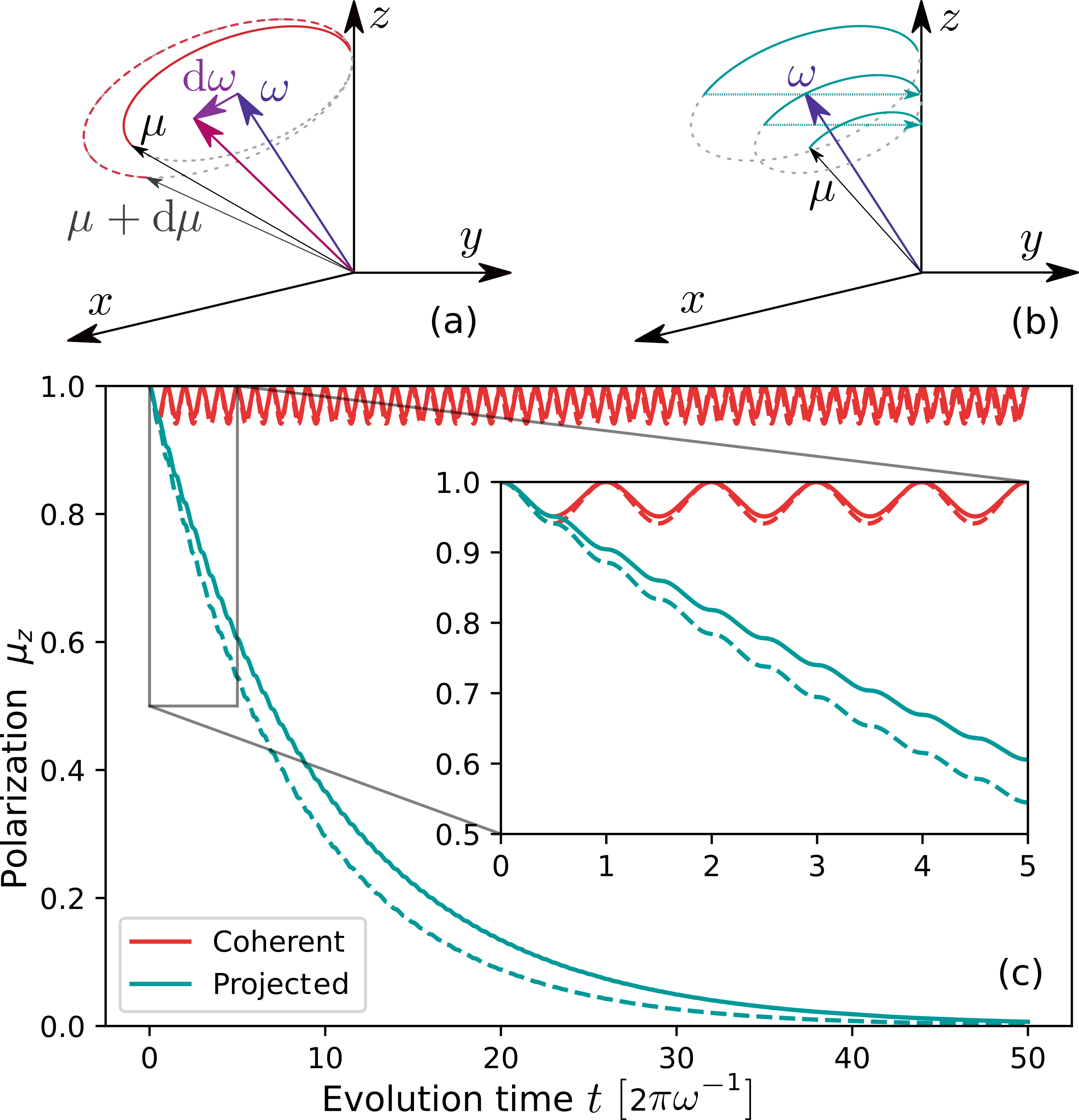
Figure 1: Comparison of the qubit-probe trajectories of the polarization vector $\boldsymbol{\mu}$ for coherent and projected evolutions for the same precesion frequency $\boldsymbol{\omega}$. (a,b) Polarization vector $\boldsymbol{\mu}$ (black vector) for coherent (solid red line) and projected evolution (solid blue line) for the same precesion frequency $\boldsymbol{\omega}$ (violet vector). The dotted lines show the continuation of the polarization trajectory. In the coherent evolution (a), a state trajectory (dashed red line) of the polarization vector $\boldsymbol{\mu}+\mathrm{d\boldsymbol{\mu}}$ (gray vector) is also shown due to a deviation $\mathrm{d}\omega_{x}$ (violet vector) on the component $\omega_{x}$ of the precession frequency leading to $\omega_{x}+\mathrm{d}\omega_{x}$ (purple-red vector). In (b) the polarization vector follows a trajectory driven by a coherent evolution until a non-demolition measurement projects its component on the z-axis. (c) Qubit-probe polarization $\mu_{z}$ along the $z$-axis as a function of time $t$, for the coherent and projected evolutions (red and blue color lines respectively) with $\omega_{x}$ and $\omega_{x}+\mathrm{d}\omega_{x}$ (solid and dashed lines respectively). We consider an offset $\omega_{z}$ that shows that the exponential decay resulting from a projected evolution induces larger differences between the evolutions corresponding to $\omega_{x}$ and $\omega_{x}+\mathrm{\mathrm{d}}\omega_{x}$, compared to the differences induced by a coherent evolution. For the schematic plots we use $\boldsymbol{\omega}=2\pi(\cos\theta,0,\sin\theta)$ with $\theta=0.9\pi/2$ being $\omega_{z}\apprge 6\omega_{x}$, $\mathrm{d}\omega_{x}=0.1\omega_{x}$, $\tau=0.5$ and $\boldsymbol{\mu}(0)=\mathbf{z}$.

The QFI of Eq. (4) can be expressed in terms of the polarization vector as

$$\mathcal{F_{Q}}(\omega_{x})=\frac{1}{1-\mu^{2}}(\partial_{\omega_{x}}\boldsymbol{\mu}_{\mathrm{r}})^{2}+(\partial_{\omega_{x}}\boldsymbol{\mu}_{\mathrm{t}})^{2}$$ , (6)

where $\partial_{\omega_{x}}\boldsymbol{\mu}_{\mathrm{r}}$ and $\partial_{\omega_{x}}\boldsymbol{\mu}_{\mathrm{t}}$ denote the radial and tangential components of the displacement $\partial_{\omega_{x}}\boldsymbol{\mu}$ (see App. A). This means that information is contained on changes on the absolute value of the polarization vector and on its direction.

III Quantum Fisher Information for a qubit-probe under coherent evolution

We analyze here the estimation protocol when the qubit sensor undergoes a coherent dynamic (Zwick et al., 2016a, b; Degen et al., 2017; Poggiali et al., 2018; Mukherjee et al., 2019; Zwick et al., 2020; Wang et al., 2020; Mu et al., 2020; Zwick and Álvarez, 2023). The QFI of the coupling strength $\omega_{x}$, obtained by measuring $\left\langle\sigma_{z}\right\rangle$ at time $t$ under a coherent free evolution, is determined by the difference between the polarization trajectories squematized in Figure 1, following Eq. (6). The dynamics of these polarization trajectories of the qubit-probe state $\boldsymbol{\mu}$ and $\boldsymbol{\mu}+d\boldsymbol{\mu}$, correspond to precessions with frequencies $\boldsymbol{\omega}$ and $\boldsymbol{\omega}+d\boldsymbol{\omega}$, with the couplings $\omega_{x}$ and $\omega_{x}+\mathrm{d}\omega_{x}$ respectively (Fig. 1a). Figure 1c shows the corresponding qubit-probe polarization $\mu_{z}$ as a function of the evolution time. Since the polarization norm is conserved during the coherent evolution, the first term in Eq. (6) vanishes, and the QFI coincides with the squared euclidean displacement induced on the polarization vector, i.e. the derivative $\partial_{\omega_{x}}\boldsymbol{\mu}_{\mathrm{r}}(t)=0$ and thus the $\mathcal{\mathcal{F_{Q}^{\mathrm{coh}}}}(\omega_{x})=(\partial_{\omega_{x}}\boldsymbol{\mu}_{\mathrm{t}}(t))^{2}$. This displacement is induced by two contributions: one due to the change in the norm of the precession frequency and the other due to the change in the precession cone (the precession axis), as shown in Fig. 1a. The later induces a periodic displacement, becoming maximal at half periods of the precession and null at every period, while the displacement induced by the former grows quadratically as a function of time and defines the more significant contribution to the QFI at long evolution times. More explicitly, the polarization vector at the evolution time $t$ is

$$\boldsymbol{\mu}(t)=\mu_{0}\begin{pmatrix}\dfrac{\omega_{x}\omega_{z}}{\omega^{2}}(1-\cos(\omega t))\\ -\dfrac{\omega_{x}}{\omega}\sin(\omega t)\\ \dfrac{\omega_{z}^{2}}{\omega^{2}}+\dfrac{\omega_{x}^{2}}{\omega^{2}}\cos(\omega t)\end{pmatrix}$$ , (7)

where $\omega=\absolutevalue{\boldsymbol{\omega}}$. The spin-state polarization on the longitudinal axis is

$$\mu_{z}(t)=\mu_{0}\alpha(t),\>\alpha(t)=\dfrac{\omega_{z}^{2}}{\omega^{2}}+\dfrac{\omega_{x}^{2}}{\omega^{2}}\cos(\omega t),$$ (8)

where $\mu_{0}$ is a constant giving the initial polarization. The longitudinal polarization $\mu_{z}(t)$ oscillates with an amplitude $\mu_{0}\omega_{x}^{2}/\omega^{2}$ with respect to its mean value $\mu_{0}\omega_{z}^{2}/\omega^{2}$ as displayed in Fig. 1.

Then, the Fisher information is

$$\mathcal{F_{Q}^{\mathrm{coh}}}(\omega_{x})=\mu_{0}^{2}\left(\dfrac{\omega_{x}^{2}}{\omega^{2}}t\begin{pmatrix}\dfrac{\omega_{z}}{\omega}\sin(\omega t)\\ -\cos(\omega t)\\ -\dfrac{\omega_{x}}{\omega}\sin(\omega t)\end{pmatrix}\right.\\ \left.+\dfrac{\omega_{z}}{\omega^{2}}\begin{pmatrix}\dfrac{\omega_{z}^{2}-\omega_{x}^{2}}{\omega^{2}}(1-\cos(\omega t))\\ -\dfrac{\omega_{z}}{\omega}\sin(\omega t)\\ -2\dfrac{\omega_{x}\omega_{z}}{\omega^{2}}(1-\cos(\omega t))\end{pmatrix}\right)^{2}\\ =\mu_{0}^{2}\dfrac{\omega_{x}^{4}}{\omega^{4}}t^{2}\left(1+\dfrac{2\omega_{z}^{2}\sin(\omega t)}{\omega_{x}^{2}\omega t}\right.\\ \left.+\left(\dfrac{\omega_{z}}{\omega_{x}^{2}t}\right)^{2}\left[(1-\cos(\omega t))^{2}+\dfrac{\omega_{z}^{2}}{\omega^{2}}\sin^{2}(\omega t)\right]\right),$$ (9)

which for long times $t\gg\frac{\omega_{z}}{\omega_{x}^{2}}$, takes the approximated form

$$\mathcal{F_{Q}^{\mathrm{coh}}}(\omega_{x})\approx\mu_{0}^{2}\left(\dfrac{\omega_{x}}{\omega}\right)^{4}t^{2},$$ (10)

that grows quadratically with time. The accompanying factor $\left(\dfrac{\omega_{x}}{\omega}\right)^{4}$ is the fourth power of the cosine of the angle $\theta$ between the precession frequency $\boldsymbol{\omega}$ and the $\mathbf{x}$ direction, $\omega_{x}=\omega\cos\theta$. The QFI as a function of $\theta$ and the evolution time shows approximatelly countourn lines given by the relation $t\propto 1/\cos^{2}\theta=1+\frac{\omega_{z}^{2}}{\omega_{x}^{2}}$, as shown in Fig. 2. Thus, the QFI of $\omega_{x}$ grows faster as the on resonance condition is approached, and tends to $0$ as $\theta\rightarrow\pi/2$ by increasing the offset.

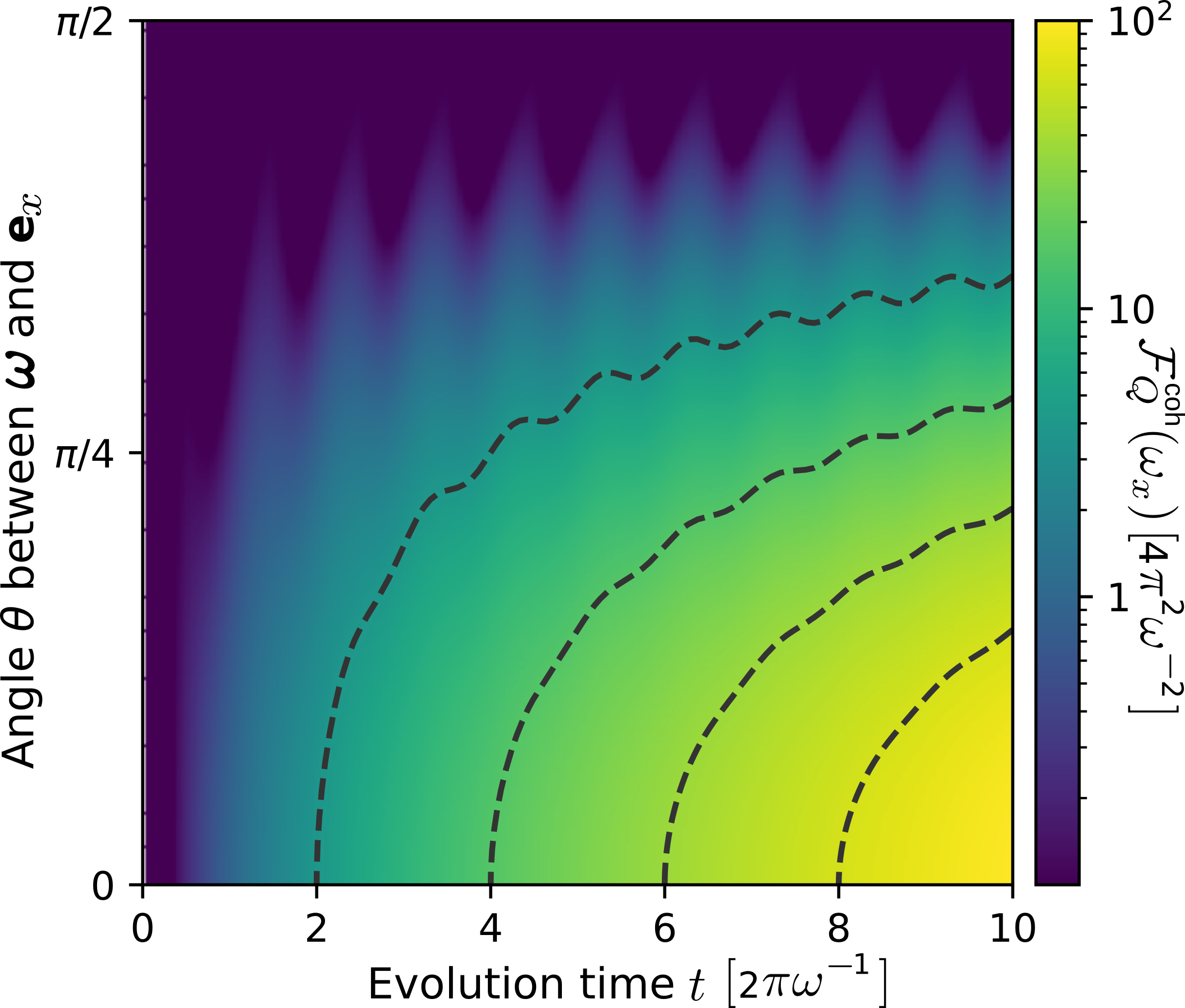
Figure 2: Quantum Fisher Information of $\omega_{x}$ as a function of the evolution time $t$ and of the angle $\theta=\arctan\left(\frac{\omega_{z}}{\omega_{x}}\right)$ between the precesion frequency vector $\boldsymbol{\omega}$ and the direction $\mathbf{x}$ for a coherent evolution from the initial state $\boldsymbol{\mu}(0)=\mathbf{z}$. The dashed lines indicate contour lines that approximatelly satisfy the relation $t\propto 1/\cos^{2}\theta$.

IV Quantum Fisher Information for a qubit-probe under projected evolution

We here analyze the estimation protocol when the qubit sensor undergoes an incoherent dynamic via projected evolutions along the $\mathbf{z}$ axis. This is achieved through periodic projective –non-demolition– measurements of the observable $\sigma_{z}$ at stroboscopic times with a delay $\tau$ (Kwiat et al., 1999; Kofman and Kurizki, 2000; Bretschneider et al., 2012; Zwick et al., 2016a; Müller et al., 2016, 2020; Zwick and Álvarez, 2023). Experimental realization of such measurements often entails applying repetitive random magnetic field gradients (Álvarez et al., 2010; Bretschneider et al., 2012) or employing stochastic processes (Dalibard et al., 1992; Nielsen et al., 1998; Teklemariam et al., 2003; Tycko, 2007; Zheng et al., 2013) on the qubit-probe system. In the case of magnetic resonance, direct projective measurements are challenging, but they can be replicated using induced dephasing techniques (Nielsen et al., 1998; Xiao and Jones, 2006; Álvarez et al., 2010; Tycko, 2007; Bretschneider et al., 2012; Zheng et al., 2013).

A schematic representation of the probe state evolution is illustrated in Fig. 1b. Immediately after the projective measurement, the qubit-probe polarization lies on the $\mathbf{z}$ axis. The transversal component is erased by the non-demolition measurement process, and thus following Eq. (7) the polarization norm is reduced by a factor $\alpha(\tau)$ as defined in Eq. (8). For an evolution time $t$ that contains $n$ stroboscopic projective measurements, $t=n\tau+\Delta t$ with $n\in\mathbb{N}$ and $\Delta t\in[0,\tau)$, the polarization $\mu_{z}$ is

$$\mu_{z}(t)=\mu_{0}\alpha(\tau)^{n}\alpha(\Delta t).$$ (11)

At the stroboscopic times $n\tau$, the polarization decays exponentially with the characteristic time

$$t_{c} =-\frac{\tau}{\ln\absolutevalue{\alpha(\tau)}}.$$ (12)

The evolution of the polarization $\mu_{z}(t)$ is shown in Fig. 1c for the precession frequencies $\boldsymbol{\omega}$ and $\boldsymbol{\omega}+d\boldsymbol{\omega}$, with the couplings $\omega_{x}$ and $\omega_{x}+\mathrm{d}\omega_{x}$ respectively as in the coherent evolution case. Notice that the projected evolution difference between the two cases is significantly larger than that for the coherent evolution case.

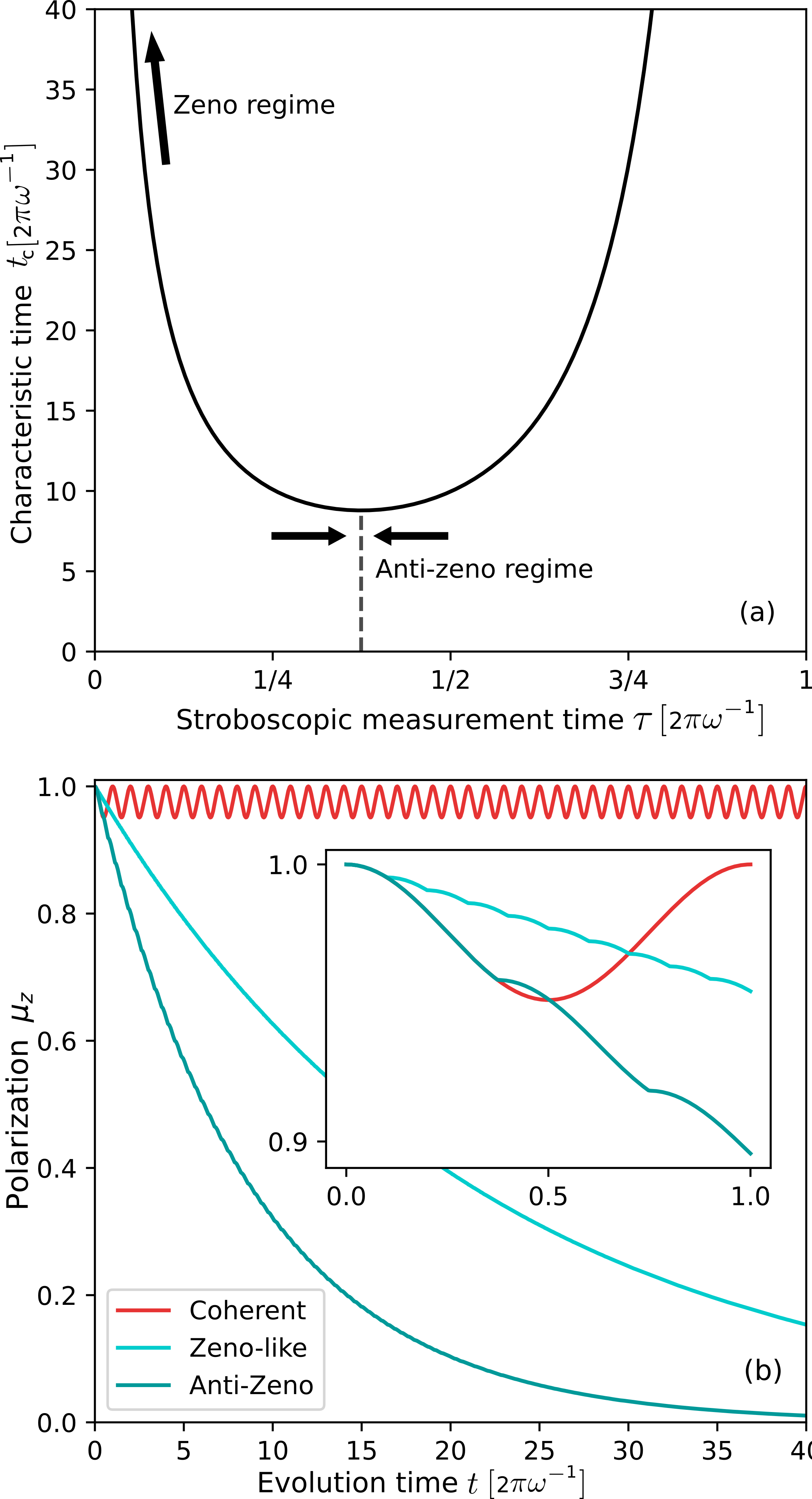
Figure 3: (a) Characteristic time $t_{c}$ of a measurement-induced decay as a function of the stroboscopic time $\tau$. The Zeno regime ocurrs when $\tau$ tends to $0$, while the Anti-Zeno regime ocurrs for the region where the characteristic time $t_{c}$ is minimum around $\tau\approx\frac{3}{8}$. For $\omega_{z}\gg\omega_{x}$, $t_{c}\approx\frac{\omega^{2}\tau}{2\omega_{x}^{2}sin^{2}(\frac{\omega\tau}{2})}$, and the minimum ocurr for $\omega\tau=\text{$\tan$}(\frac{\omega\tau}{2})$. (b) Polarization $\mu_{z}$ along the $z$-axis as a function of the total evolution time, for coherent and two projective evolutions corresponding to a Zeno ($\tau=0.1$) and Anti-Zeno regime ($\tau\approx\frac{3}{8}$) (red, blue and cyan color lines respectivesly). Here $\boldsymbol{\omega}=2\pi(\cos\theta,0,\sin\theta)$ with $\theta=0.9\pi/2$ being $\omega_{z}\apprge 6\omega_{x}$, $\boldsymbol{\mu}(0)=\mathbf{z}$.

Figure 3a shows the decay time $t_{c}$ as a function of the stroboscopic measurement time $\tau$ for $\omega_{z}\apprge 6\omega_{x}$. A similar qualitative behavior is seen in general for $\omega_{z}>\omega_{x}$, as the polarization state $\boldsymbol{\mu}$ does not cross the $\mu_{z}=0$ plane during its evolution. As the stroboscopic time $\tau\rightarrow 0$, the evolution of the polarization factor $\alpha(\tau)\rightarrow 1$ and thus the characteristic decay time $t_{c}\rightarrow\infty$ defining the Zeno regime where the QZE is manifested (Misra and Sudarshan, 1977; Kofman and Kurizki, 2000). Figure 3a also shows a region for values of $\tau$, where the decay time $t_{c}$ is minimal corresponding to a Anti-Zeno regime (Kofman and Kurizki, 2000). These Zeno and Anti-Zeno regimes induce the slowest and fastest exponential decay of the polarization $\mu_{z}$ evolution under stroboscopic measurements as shown in Fig. 3b.

We now calculate the QFI from Eq. (6). Due to the reduction of the polarization norm by the factor $\alpha(\tau)$ at every projective measurement, the first term in Eq. (6) becomes a piecewise constant evolution. The coherent evolution between the projective measurements contributes to the QFI via the second term of Eq. (6) with a value equal to the one of a coherent evolution after the projection. Thus the second term of the QFI is a coherent contribution that only adds a small quantity on top of the main overall information given by the first term due to the incoherent evolution counterpart. If the stroboscopic time $\tau$ is small, $\omega\tau\ll 2\pi$, the first term of the QFI is generated by a decaying incoherent evolution of the qubit-state $\mu_{z}$. The QFI at the stroboscopic times $t=n\tau$ is given only by the radial –first– term in Eq. (6). This is regardless of the value of $\omega_{x}$, as all trajectories at those specific times are along the $\mathbf{z}$ axis (see Fig. 1b). Furthermore, during the coherent evolution between the projective measurements, since the polarization vector conserves its norm, the radial term remains constant, and the second term takes the usual form for a coherent evolution as described in Sec. III, with an initial polarization given by the one obtained at the last projective measurement. Hence, the QFI may be approximated by the first term of Eq. (6) up to a difference of $\mu_{0}^{2}\alpha(\tau)^{2n}\Delta t^{2}$, where $\Delta t$ is the elapsed time after the last measurement. Considering this approximation, the QFI takes the form (see App. B)

$$\mathcal{F_{Q}^{\mathrm{proj}}}(\omega_{x}) =t^{2}\mu_{0}^{2}\frac{1}{\tau^{2}}\frac{\alpha(\tau)^{2(t/\tau-1)}}{1-\mu_{0}^{2}\alpha(\tau)^{2t/\tau}}(\partial_{\omega_{x}}\alpha(\tau))^{2}.$$ (13)

The QFI as a function of time for this projected evolution is represented by a family of self-similar functions parameterized by $\boldsymbol{\omega}$ and $\tau$. Figure 4 shows this QFI of the coupling strength $\omega_{x}$ as a function of stroboscopic time $\tau$ and the total evolution time $t$. The dashed line in Fig. 4(a) shows the maximum value of the QFI $\mathcal{F_{Q\mathrm{,max}}^{\mathrm{proj}}}=\mathcal{\mathcal{F_{Q}^{\mathrm{proj}}}}(t_{\text{{max} }})$ obtained at $t_{\text{{max} }}$ that satisfies $\partial_{t}\mathcal{\mathcal{F_{Q}^{\mathrm{proj}}}}(t_{\text{{max} }})=0$. The maximum QFI ocurr at

$$t_{\text{{max} }} =\xi(\mu_{0})t_{c}, \xi(\mu_{0}) =1+\frac{1}{2}\operatorname{W}(-2\mu_{0}^{2}/\mathrm{e^{2}}),$$ (14)

where $\operatorname{W}$ is the principal branch of the Lambert’s W function and vary monotonically from $0.79$ to $1$ as $\mu_{0}$ goes from $1$ to $0$. Then the maximum QFI is given by

$$\mathcal{\mathcal{F_{Q\mathrm{,max}}^{\mathrm{proj}}}} =\varphi(\mu_{0})\frac{t_{c}^{2}}{\alpha(\tau)^{2}}\frac{\omega_{x}^{2}}{\omega^{2}}\left[2\frac{1-\cos(\omega\tau)}{\omega\tau}\frac{\omega_{z}^{2}}{\omega^{2}}+\sin(\omega\tau)\frac{\omega_{x}^{2}}{\omega^{2}}\right],$$ (15)

$$\varphi(\mu_{0}) =\mu_{0}^{2}\frac{(\xi(\mu_{0}))^{2}}{\mathrm{e^{2\xi(\mu_{0})}-\mu_{0}^{2}}},$$

and the behaviour of $F_{Q\mathrm{,max}}^{\mathrm{proj}}(\omega_{x})$ as a function of $\tau$ is shown in Fig. 4(b).

Approaching the Zeno regime $\omega\tau\rightarrow 0$, $\alpha(t)\approx 1-\omega_{x}^{2}t^{2}$ and the QFI $\mathcal{F_{Q\mathrm{,max}}^{\mathrm{proj}}}\rightarrow 4\varphi(\mu_{0})/\omega_{x}^{2}$ is a constant value that is obtained at $t_{\text{{max} }}\approx\frac{\xi(\mu_{0})}{\omega_{x}^{2}\tau}$, where both are independent of $\omega_{z}$. This is an important feature of the QZE estimation strategy, as it does not require previous knowledge of the offset $\omega_{z}$ to make an efficient inference. For large offsets $\omega_{z}\gg\omega_{x}$, this constant value for $\mathcal{F_{Q\mathrm{,max}}^{\mathrm{proj}}}$ is extended to the Anti-Zeno regime requiring less total evolution time to be achieved as can be observed in Fig. 4. Notice that outside the QZE regime, previous knowledge of the offset is needed for an efficient estimation of the coupling. By continuing to increase $\tau$, the $\mathcal{F_{Q\mathrm{,max}}^{\mathrm{proj}}}$ decreases to zero. This could be related to the manifestation of critical phenomena in the extractable information defining transitions between dynamic regimes of the sensor (Zwick et al., 2016b). Then, $\mathcal{F_{Q\mathrm{,max}}^{\mathrm{proj}}}$ rapidily increases as the evolution approaches the coherent regime, i.e. for $\tau\rightarrow 2\pi\omega^{-1}$, but it requires a total evolution time orders of magnitude larger than its Anti-Zeno counterpart.

It is worth noting that the functional form of $\mathcal{F_{Q\mathrm{,max}}^{\mathrm{proj}}}$ differs from that of the level curves for the QFI in a coherent evolution, as illustrated in Fig. 2 compared to Fig. 4. Specifically, for sufficient large values of $\omega_{z}$, $\mathcal{F_{Q\mathrm{,max}}^{\mathrm{proj}}}$ becomes constant and defines a contour line that gives the higher information gain at an earlier time compared to the corresponding contour line determined from a coherent evolution.

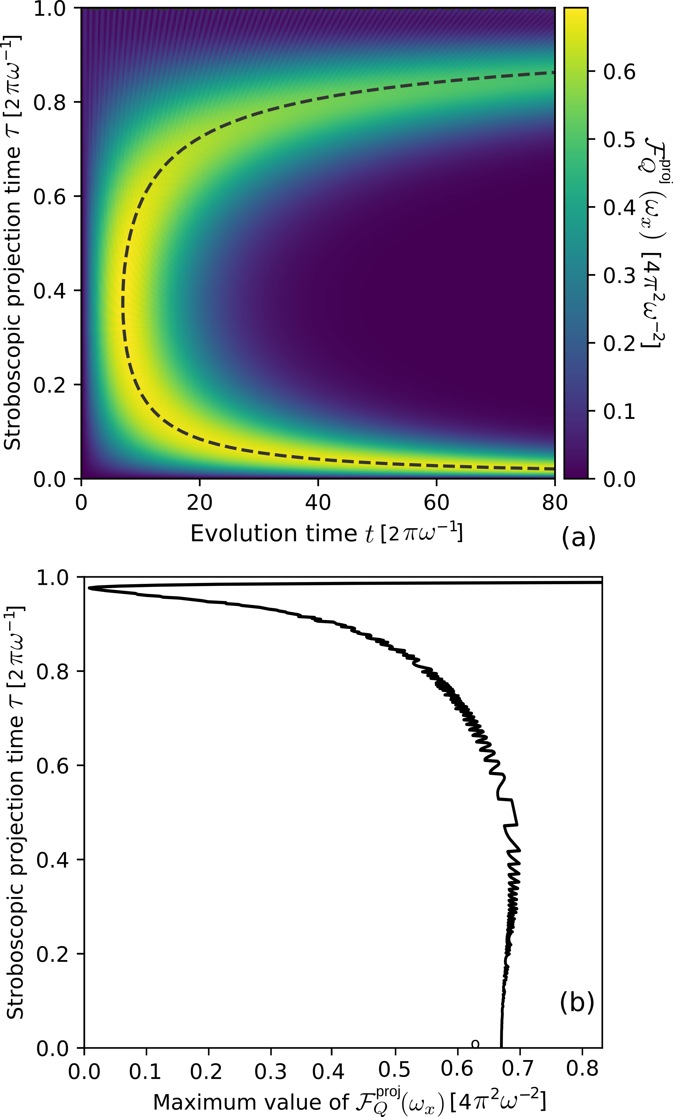
Figure 4: Quantum Fisher information of the coupling strength $\omega_{x}$ for the projected evolution of the quantum-probe. (a) The QFI $\mathcal{F_{Q}}(\omega_{x})$ as a function of the stroboscopic measurement time $\tau$ and the total evolution time $t$. The dashed line shows the maximum value of the QFI $\mathcal{F_{Q\mathrm{,max}}^{\mathrm{proj}}}=\mathcal{\mathcal{F_{Q}^{\mathrm{proj}}}}(t_{\text{{max} }})$ obtained at $t_{\text{{max}}}$. (b) Maximum QFI $\mathcal{F_{Q\mathrm{,max}}^{\mathrm{proj}}}$ as a function of $\tau$. The vertical axes in both panels represents the stroboscopic time $\tau$. Parameters used for the plot: $\boldsymbol{\omega}=2\pi(\cos\theta,0,\sin\theta)$ with $\theta=0.9\pi/2$ being $\omega_{z}\apprge 6\omega_{x}$ and $\boldsymbol{\mu}(0)=\mathbf{z}$. The oscillations in (b) are due to the finite numerical calculations.

V Maximizing Information with the Quantum-Zeno Effect

Here, we compare the estimation efficiency of the coupling strength $\omega_{x}$, when the qubit-probe undergoes coherent and projected (incoherent) evolutions. In the off-resonance regime ($\omega_{z}>\omega_{x}$,) the difference between the evolution trajectories of the observable $\mu_{z}$ for a small deviation on the precession frequency $\omega_{x}$ becomes barely distinguishable during coherent evolution (see Fig. 1c). On the contrary, projected evolutions leads to larger differences between these trajectories in a region of times before the decaying signal is lost (see Fig. 1c). As previously discussed in Eq. (5), the differences observed in the trajectories resulting from a small deviation in the parameter $\omega_{x}$ can provide valuable information about it. Figure 5 compares the time-dependent QFI of $\omega_{x}$ between a coherent ($\mathcal{F_{Q}^{\mathrm{coh}}})$ and projected ($\mathcal{F_{Q}^{\mathrm{proj}}}$) evolution estimation process, illustrating a representative functional behavior for a case with a large offset.

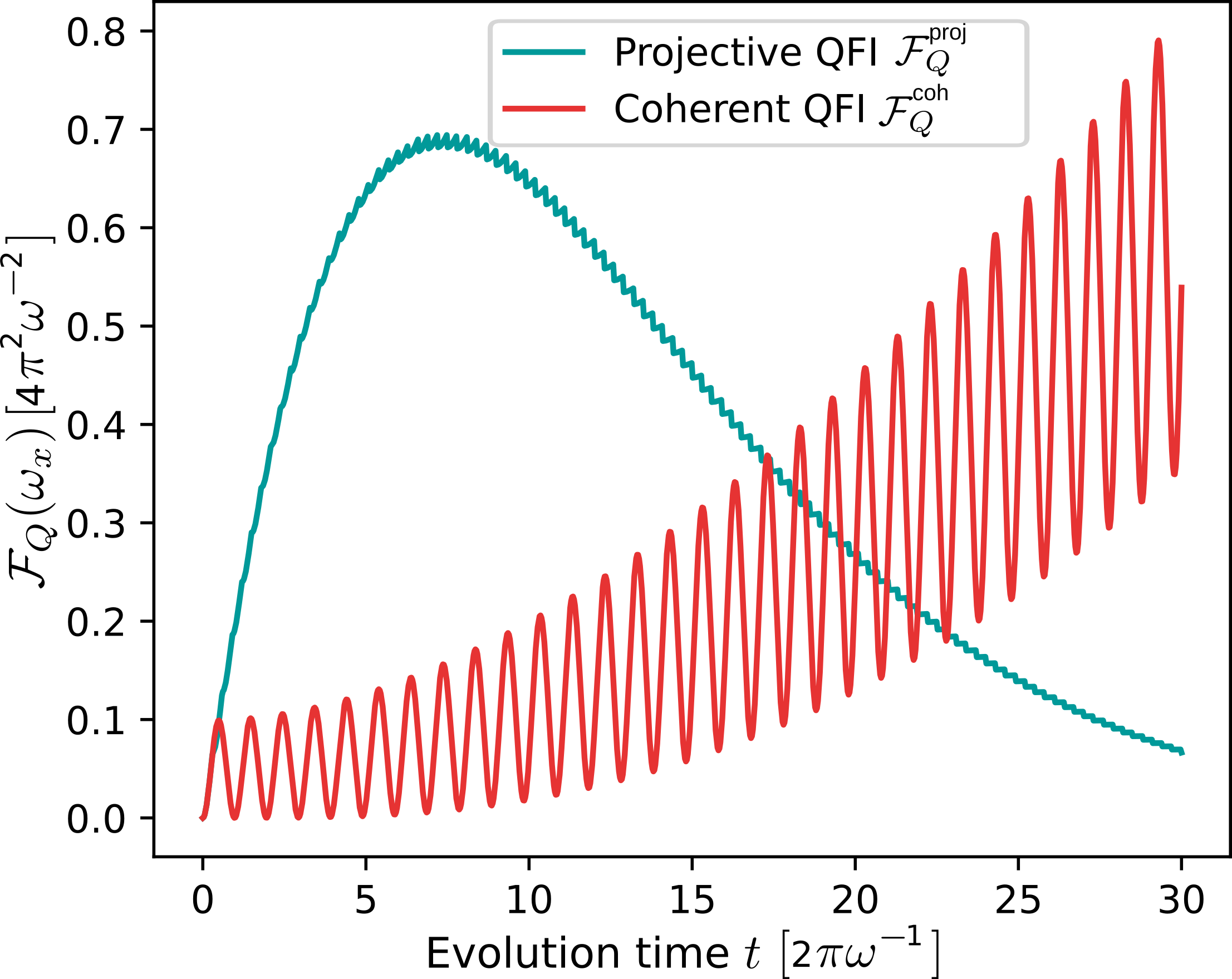
Figure 5: QFI for a large offset $\omega_{z}\apprge 6\omega_{x}$ for both coherent and projective evolution estimation. Although the QFI extracted from a coherent evolution yield higher information at long time, the QFI extracted from projective evolution yields a higher value at shorter times. The parameter used for the plot are: $\boldsymbol{\omega}=2\pi(\cos\theta,0,\sin\theta)$ with $\theta=0.9\pi/2$ being $\omega_{z}\apprge 6\omega_{x}$, $\tau=0.3$ and $\boldsymbol{\mu}(0)=\mathbf{z}$.

It reflects the key predicted results of this article: the QFI $\mathcal{F_{Q}^{\mathrm{proj}}}$ extracted from projected evolutions achieves higher values at shorter times compared to the the QFI information $\mathcal{F_{Q}^{\mathrm{coh}}}$ extracted from a coherent free evolution when the offset is large $\omega_{z}>\omega_{x}$.

The $\mathcal{F_{Q}^{\mathrm{proj}}}$reaches a maximum and then it decays, while $\mathcal{F_{Q}^{\mathrm{coh}}}$ continuously grows as a function of time, as predicted in Eq. (10). This happens because the observable longitudinal polarization $\mu_{z}$ exponentially decays to zero under projective evolutions, thus reducing the QFI after some time, while the coherent evolution preserve the polarization magnitude along time thus allowing to increse the QFI indefinitely. However, the QFI can indefinitely grow only under very ideal conditions, where the qubit-probe does not suffer decoherence.

In a realistic experiments, there is always decoherent effects that, depending the setup, can be characterized by the relaxation times $T_{1}$ or $T_{2}$, which are typically comparable to the precession period $2\pi\omega^{-1}$ or one/two orders of magnitude larger. This relaxation reduces the polarization $\mu_{z}$ by an exponential decaying factor $e^{-t/T_{1}}$ or $e^{-t/T_{2}}$ respectively. Therefore in general the maximal QFI that can be achieved for given values of $\omega_{x}$ and the offset $\omega_{z}$, is obtained by an optimal tradeoff between the ideal information gain from the qubit-probe evolution and the total available time determined by sources of relaxation. Thus, due to decoherence effects on the qubit-probe, achieving the maximal QFI in the shortest possible time is crucial.

We thus determine the maximum attainable QFI within the time interval $[0,\,t]$ for the coherent $F_{Q}^{\mathrm{coh}}$ and the projected $F_{Q}^{\mathrm{proj}}$ evolution estimations. We compare them with the quotient

$$\frac{\mathcal{\mathcal{F_{Q\mathrm{,max}}^{\mathrm{proj}}}}}{\mathcal{F_{Q\mathrm{,max}}^{\mathrm{coh}}}} =\frac{4\varphi(\mu_{0})}{\mu_{0}^{2}}\frac{\omega^{4}}{\omega_{x}^{6}}\frac{1}{t^{2}},$$ (16)

considering the approximations derived above, where $\mathcal{F_{Q\mathrm{,max}}^{\mathrm{coh}}}(\omega_{x})\approx\mu_{0}^{2}\left(\dfrac{\omega_{x}}{\omega}\right)^{4}t^{2}$ for $t\gg\frac{\omega_{z}}{\omega_{x}^{2}}$ and $\mathcal{F_{Q\mathrm{,max}}^{\mathrm{proj}}}\approx 4\varphi(\mu_{0})/\omega_{x}^{2}$ for large offsets $\omega_{z}\gg\omega_{x}$ and $\tau\lesssim 0.6$. This expression thus defines the conditions for the optimal estimation at the total available evolution time $t$. The estimation procedure based on projective measurements on the qubit-probe maximize the information about $\omega_{x}$ when the available time is

$$t <\frac{2\sqrt{\varphi(\mu_{0})}}{\mu_{0}\omega_{x}}\left(1+\frac{\omega_{z}^{2}}{\omega_{x}^{2}}\right).$$ (17)

In the limit of low polarization $\mu_{0}\ll 1$, $\varphi(\mu_{0})=e^{-2}\mu_{0}^{2}$, and Eq. (17) aproximates to

$$t<\frac{2e}{\omega_{x}}\left(1+\frac{\omega_{z}^{2}}{\omega_{x}^{2}}\right),$$ (18)

which is independent of the particular initial polarization $\mu_{0}$.

Figure 6 shows the quotient of Eq. (16) as a function of the angle $\theta=\arctan\left(\frac{\omega_{z}}{\omega_{x}}\right)$ of $\boldsymbol{\omega}$ with respect to the $x$ axis and the total available time $t$. Areas colored in white indicate when the quotient is equal to $1$, thereby defining the boundary between the parametric region where projected or coherent evolution is more efficient por the parameter estimation. For values of $\omega_{z}$ where the quotient is above $1$, the projected evolution estimation is expected to perform better, while the opposite is expected for values below it. This dividing boundary curve is approximated by the relation $\omega_{z}\propto\omega_{x}\sqrt{\omega_{x}t-1}$, provided that $t\geq t_{\text{{max}}}$. For values of $\omega_{z}$ above this boundary region, the offset is so strong that the contribution of $\omega_{x}$ to the oscillatory dynamics requires more time than is available. Consequently, coherent evolution does not provide a better estimation compared to that extracted from the incoherent decaying dynamics of the qubit-probe polarization. When the offset is below this boundary region, the oscillatory coherent evolution of the quantum-probe is sensitive enough to provide a larger QFI than the maximum attainable by the incoherent evolution.

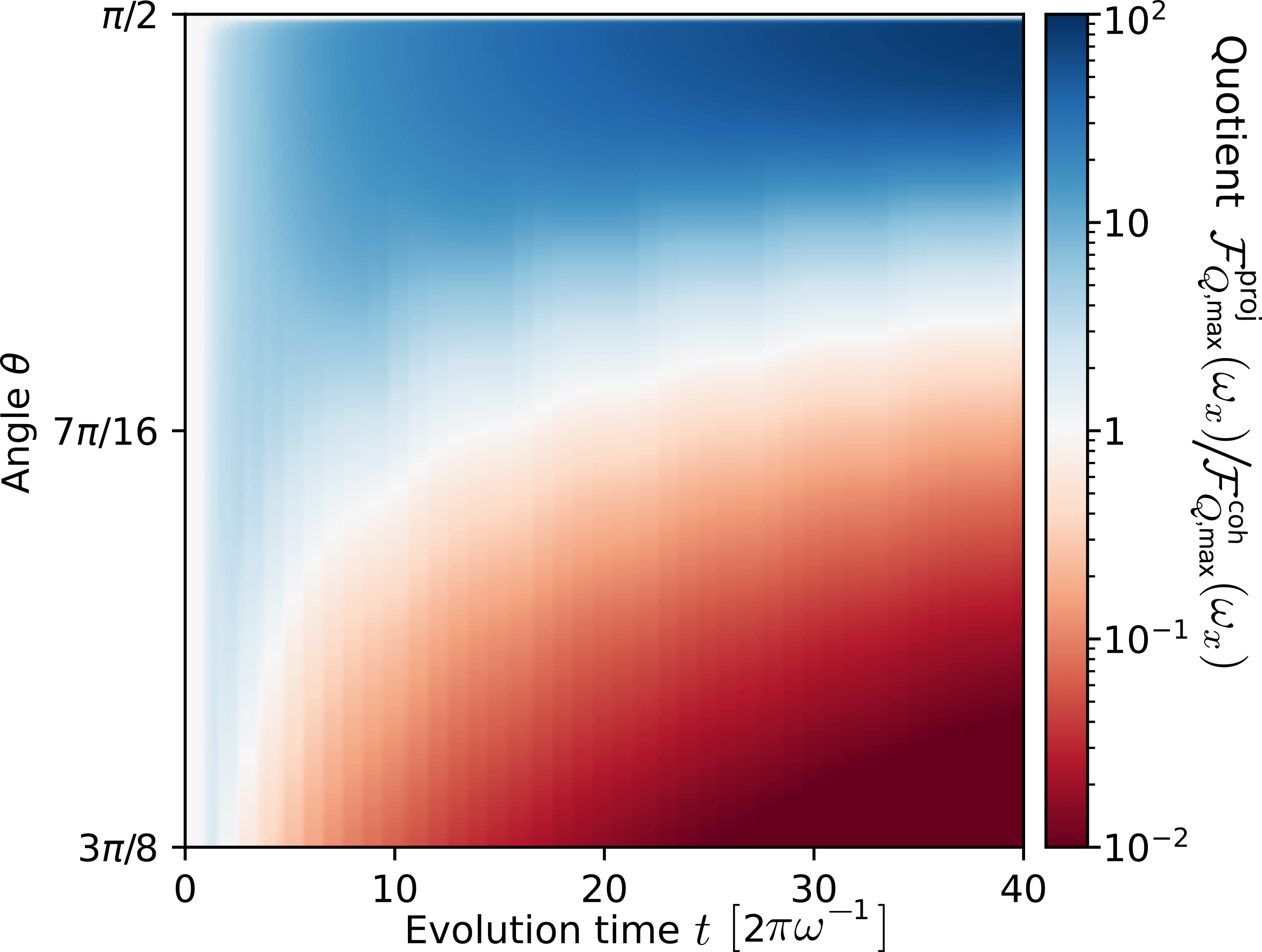
Figure 6: Quotient of the maximum obtainable QFI for projective and coherent estimation as a function of the angle $\theta=\arctan\left(\frac{\omega_{z}}{\omega_{x}}\right)$ of $\boldsymbol{\omega}$ with respect to $\mathbf{z}$ and total available time $t$. The white color region corresponds to equal QFI that divides the region where either estimation protocol is better.

VI Applications

In this section we present physical examples that illustrate the advantages of implementing the QZE inference protocol over the coherent strategy. We begin by demonstrating the direct application of inferring AC magnetic fields that are off resonant with the qubit-probe. Subsequently, we explore how the same concept can be exploited for inferring spin-spin couplings. In the latter case, we start with the simplest case of a two-spin coupled system, followed by an example illustrating its extension to a three spin system. Finally, we generalize the approach to include many-spins.

The incoherent control necessary to achieve the Zeno effects may be applied through quantum non-demolition (QND) projective measurements (Zwick et al., 2016a), as discussed in previous sections, and/or by induced dephasing that mimics QND measurements (Álvarez et al., 2010; Bretschneider et al., 2012; Nielsen et al., 1998; Cory et al., 2000; Xiao and Jones, 2006; Zheng et al., 2013). This induced dephasing, which repetitively and stroboscopically projects the qubit state, can be achieved using various methods, including random magnetic field gradients (Álvarez et al., 2010; Bretschneider et al., 2012; Xiao and Jones, 2006), $T_{2}$ relaxation (Nielsen et al., 1998), or stochastic interactions (Tycko, 2007; Dalibard et al., 1992; Teklemariam et al., 2003). It is important to note that the results of QND measurements do not necessitate a readout, as these measurements solely guide the evolution of the qubit-probe state.

VI.1 Sensing an off-resonant, external AC magnetic field with a 1/2-spin

We consider a $1/2$-spin interacting with a homogeneous and static magnetic field $\mathbf{B}_{0}=B_{0}\mathbf{z}$ as the qubit-probe. It thus precesses with the Larmor frequency $\omega_{0}=\gamma B_{0}$ around the $\mathbf{z}$ axis, where $\gamma$ is the gyromagnetic ratio. The qubit-probe is treated as a magnetometer for estimating an AC magnetic field along the $\mathbf{x}$ axis, determined by $\mathbf{B}_{1}(t)=2B_{1}\cos(\omega t)\mathbf{x}$, where $\omega$ is the carrier frequency and $B_{1}$ is the field strength (Degen et al., 2017; Boss et al., 2017; Schmitt et al., 2017; Glenn et al., 2018; Jiang et al., 2023; Segawa and Igarashi, 2023). In the rotating frame precessing at the angular frequency $\omega$, and under the rotating wave approximation (Slichter, 1990), the spin interacts with an effective magnetic field $(\omega_{0}-\omega)/\gamma\mathbf{z}+B_{1}\mathbf{x}$. Here, we have assumed that $B_{0}\gg B_{1}$ and that the offset $\omega_{z}=\omega_{0}-\omega$ is much lower than the Larmor frequency $\left|\omega_{z}\right|\ll\omega_{0}$.

This interaction can thus be map to the general two-level system Hamiltonian of Eq. (1), where $\omega_{x}=\gamma B_{1}$, $\omega_{y}=0$ and the offset $\omega_{z}=\gamma B_{0}-\omega$ defines how far the AC field is from the on-resonance condition.

Following the results derived in Eqs. (16)-(18), we can determine when the projective measurements protocol for estimating the AC field strength $\omega_{x}=\gamma B_{1}$ provides a better approach compared to a coherent evolution if the available total measurement time is $t$. We thus obtain that if $t$ satisfies

$$t<2e\frac{B_{1}^{2}+(B_{0}-\omega/\gamma)^{2}}{B_{1}^{3}},$$ (19)

projective measurement outperforms a coherent evolution estimation protocol. This regime is useful when the on-resonance condition cannot be fulfilled, which might occur when either $\omega$ or $B_{0}$ cannot be controlled to put the qubit-probe on resonance. For example, this circumstance could arise when using an ensemble of spins that feel different magnetic fields $B_{0}$, leading to an intrinsic large offset value. This condition can arise in Nuclear Magnetic Resonance (NMR) experiments using a mouse magnet that is placed at the side or near the surface of the sample to be studied, causing the $B_{0}$ field to be spacially inhomogeneous within the sample, leading to a broadening of the NMR spectrum (Perlo et al., 2005).

VI.2 Sensing spin-spin couplings

The estimation of the coupling strength between interacting spins is a crucial experimental challenge in chemistry for characterizing molecular topology and various quantum technologies (Braunschweiler and Ernst, 1983; Caravatti et al., 1983; Ernst et al., 1990; Luy et al., 1999; Tycko, 2007; Bretschneider et al., 2012; Shi et al., 2013; Degen et al., 2017). This is particularly relevant for Hamiltonian characterization (Caravatti et al., 1983; Ernst et al., 1990; Tycko, 2007; Segawa and Igarashi, 2023; Degen et al., 2017; Bretschneider et al., 2012) as well as the improvement of spectroscopy techniques (Lang et al., 2015; Smith et al., 2012; Jiang et al., 2023; Schmitt et al., 2017; Glenn et al., 2018; Boss et al., 2017), optimization of hyperpolarization in NV centers (King et al., 2015; Rao and Suter, 2020; Wang et al., 2013; Álvarez et al., 2015; Broadway et al., 2016; Ajoy et al., 2018; Zangara et al., 2019) and NMR (Pravdivtsev et al., 2013, 2014a; Ivanov et al., 2014; Pravdivtsev et al., 2014b), cross-polarization (Chattah et al., 2003; Álvarez et al., 2006; Raya et al., 2011; Harris et al., 2012; Raya et al., 2013; Raya and Hirschinger, 2017; Hirschinger and Raya, 2023), the characteriation of molecular structures with NMR that define physicochemistry properties or inter-nuclear distances (Slichter, 1990; Müller et al., 1974; Bretschneider et al., 2012; Shi et al., 2013), among others.

VI.2.1 Two-spin coupling

To illustrate the introduced inference method, we focus on estimating the coupling strength and inferring the Hamiltonian of two interacting spins systems. Specifically, we consider a two-spin coupled system during a cross-polarization experiment in NMR (Hartmann and Hahn, 1962; Müller et al., 1974). This technique is useful for transferring magnetization from a system with high abundance and/or polarization (spin $I$), such as ${}^{1}H$, to a system of low abundance and/or small gyromagnetic factor $\gamma$ (spin S), like ${}^{13}C$. The two spin species are subjected to a static magnetic field $B_{0}$ as in the previous example.

The Zeeman interaction defines the resonance frequencies of each spin $\omega_{0,\,i}=\gamma_{i}B_{0}$ where $i=I,S$, typically in the order of hundreds of MHz and differing also in that order. The dipolar interaction between the spins is in the order of kHz, making the polarization/magnetization exchange between them negligible. To generate the polarization exchange (cross polarization), it is necessary to put the two spin species on resonance. For that, oscillating magnetic fields $\mathbf{B}_{1,i}(t)$ of frequences $\omega_{0,\,i}$ ($i=I,S$) are applied. In the high radio frequency field regime where $\left|\omega_{1,\,I}+\omega_{1,\,S}\right|\gg\left|b\right|$ with $\omega_{1,\,i}=\gamma_{i}B_{1,i}$ and $B_{1,i}=\max\left|\mathbf{B}_{1,i}(t)\right|$, a secular approximation can be done (Müller et al., 1974). This yields the interacting Hamiltonian in the double rotating frame precessing at the two spin frequencies

$$H =-\frac{1}{2}\Delta\left(S_{z}-I_{z}\right)+b\left(S_{x}I_{x}+S_{y}I_{y}\right).$$ (20)

Here $I_{v}=\frac{1}{2}\sigma_{v,I}$ and $S_{v}=\frac{1}{2}\sigma_{v,S}$ are the spin operators with $v=x,y,z$, $\Delta=\left(\omega_{1,\,S}-\omega_{1,\,I}\right)$ is the off-resonant energy, and the dipolar interaction is

$$b =-\frac{1}{2}\left(\frac{\mu_{0}\gamma_{I}\gamma_{S}}{4\pi r^{3}}\right)\frac{3r_{z}^{2}-r^{2}}{r^{2}},$$ (21)

where $r$ is the modulus of the internuclear distance vector, and $r_{z}$ its $z$ component. Then, the on-resonance condition for achieving a full cross-polarization, called the Hartmann-Hahn condition (Hartmann and Hahn, 1962), is $\Delta=0$.

The sample is initially polarized by the action of the static field $B_{0}\mathbf{z}$. The polarization in the insensitive species $S$ is typically negligible or removed for quantitative analisis, so only the sensitive species $I$ is polarized along $\mathbf{z}$-axis according to the Boltzmann distribution. The initial state is diagonal in the Zeeman basis, and as the Hamiltonian of Eq. (20) conserves the total magnetization on the $\mathbf{z}$-axis, the evolution of the spins takes place within density matrix blocks conserving the total magnetization $S^{z}+I^{z}$. The matrix blocks of the spaces $\{{\uparrow\uparrow}\}$ and $\{{\downarrow\downarrow}\}$ do not generate dynamics in the system, so their populations are constant over time. The dynamics ocurr only on the subspace of the Zeeman states $\{\uparrow\downarrow,\,\downarrow\uparrow\}$, subject to the effective Hamiltonian

$$\frac{1}{2}\begin{pmatrix}-\Delta&b\\ b&\Delta\end{pmatrix}.$$ (22)

This Hamiltonian is equivalent to Eq. (1), with an angular frequency

$$\boldsymbol{\omega} =\frac{1}{\hbar}(-b,\,0,\,\Delta),$$ (23)

with a pauli operator $\boldsymbol{\sigma}_{\uparrow\downarrow}$ acting on the two state subspace $\{\ket{\uparrow\downarrow},\,\ket{\downarrow\uparrow}\}$. Then, the process to estimate the coupling strength $b$ is analogous to the estimation of $\omega_{x}$ with an offset $\omega_{z}=\Delta$ as discussed in the previous sections.

Since the blocks of the spaces $\{\uparrow\uparrow\}$ and $\{\downarrow\downarrow\}$ are static, they do not contribute to the QFI of any parameter. Only the state in the block of space $\{\uparrow\downarrow,\,\downarrow\uparrow\}$ contributes to the QFI. In this two-level space, whith a trace of $\frac{1}{2}$, the polarization vector is defined by

$$\rho_{\uparrow\downarrow} =\frac{1}{4}\left[\mathrm{I}_{\uparrow\downarrow}+\boldsymbol{\mathfrak{\mu}}\cdot\boldsymbol{\sigma}_{\uparrow\downarrow}\right],$$ (24)

where the subscript $\uparrow\downarrow$ indicates that the operators act on the subspace generated by $\{\ket{\uparrow\downarrow},\,\ket{\downarrow\uparrow}\}$. The initial condition is

$$\boldsymbol{\mu}(t=0) =\left(\frac{\exp\left(-\frac{1}{2}\frac{\omega_{0,\,I}}{kT}\right)}{\cosh\left(-\frac{1}{2}\frac{\omega_{0,\,I}}{kT}\right)}-1\right)\,\mathbf{z}$$ (25)

$$\approx-\frac{1}{2}\frac{\omega_{0,\,I}}{kT}\,\mathbf{z},$$ (26)

where this last approximation corresponds to the high temperature limit, valid for NMR experiments at room temperature (Slichter, 1990). Thus the polarization vector precesses with the angular frequency, leading to an evolution for its $z$ component given by

$$\mathfrak{\mu}_{z}(t) =\frac{1}{2}\mu_{0}\frac{\Delta^{2}+b^{2}\cos(\sqrt{b^{2}+\Delta^{2}}t)}{\Delta^{2}+b^{2}}.$$ (27)

This polarization component represents the magnetization exchange between the spins, whose polarization transfer amplitude is $b^{2}/\left(\Delta^{2}+b^{2}\right)$. Therefore, an off-resonant offset $\Delta$ far from the Hartmann-Hahn condition reduces the information gain for the estimation of $b$ based on the free coherent evolution of the system. For an off-resonant exchange of polarization, with large offset $\Delta$, projective measurements applied on the spins on the z axis lead to a more efficient estimation of the coupling strength $b$ if the available total evolution time satisfies

$$t <2\mathrm{e}\frac{b^{2}+\Delta^{2}}{b^{3}}=2\mathrm{e}\frac{b^{2}+\left(\omega_{1,\,I}+\omega_{1,\,S}\right)^{2}}{b^{3}},$$ (28)

according to Eqs. (16)-(18). Typically the coherent evolution decoheres due to interactions with the environment, imposing restrictions to the available time for the inference (Chattah et al., 2003; Álvarez et al., 2006, 2007).

The impossibility of generating the Hartmann-Hahn condition occurs in many experimental situations, particularly in cases of very complex spectra, such as spin ensembles with different resonance frequencies, as is the case of solid-state systems with polycrystalline samples (Raya et al., 2011; Harris et al., 2012; Raya et al., 2013). In such cases, it is convenient to use the estimation method based on exploiting projective evolutions, which can be implemented with magnetic field gradients, as shown in Ref. (Álvarez and Suter, 2010; Xiao and Jones, 2006; Bretschneider et al., 2012). Regardless of choosing the optimal way to estimate the coupling between the spins, working in the QZE regime using projective measurements allows us to estimate the coupling selectively without needing to know the offset of the Hartmann-Hahn condition. This is a great advantage in these complex systems.

VI.2.2 Three-spin couplings

We now extend our focus to estimating the interacting couplings among three spins. Specifically, we assume one spin $S$ and two spin $I$ again in the presence of a static field $B_{0}$ in the $z$ direction and radiofrequency fields $B_{1,I}$ and $B_{1,S}$ in the $x$ direction. The dipolar couplings between $S$ and both spins $I$ are denoted as $b_{k}$, $k=1,2$, while the coupling between the spins $I$ is denoted as $d$. For a three-spin system, as in an extended cross-polarization experiment,$S$ represents for example a ${}^{13}C$ nucleus and the two spins $I$, e.g. two protons ${}^{1}H$ (Chattah et al., 2003; Raya et al., 2011, 2013; Raya and Hirschinger, 2017; Hirschinger and Raya, 2023). The dipolar couplings between the proton $k$ and the carbon are

$$b_{k} =-\frac{1}{2}\left(\frac{\mu_{0}\gamma_{I}\gamma_{S}}{4\pi r_{(k)}^{3}}\right)\frac{3r_{(k)z}^{2}-r_{(k)}^{2}}{r_{(k)}^{2}}, k=1,2,$$ (29)

and the coupling between the protons is

$$d =-\frac{1}{2}\left(\frac{\mu_{0}\gamma_{I}^{2}}{4\pi r^{3}}\right)\frac{3r_{z}^{2}-r^{2}}{r^{2}}.$$ (30)

Similar to the two coupled spins case (Sec. VI.2.1), the Hamiltonian in the double rotating frame preserves the total magnetization of the system along the respective directions of the radiofrequency fields. The Hamiltonian again acquires a block structure defined by the total magnetization along $z$ of the full system $M=M_{I}+M_{S}$, where $M_{I}=M_{1}+M_{2}$ is the total magnetization of the protons along $z$ with $M_{1}$ and $M_{2}$ being the $z$-magnetization of each proton, and $M_{S}$ is the $z$-magnetization of the ${}^{13}\mathrm{C}$. The Hamiltonian induces transitions only between states of the form $\{\ket{M_{I},\,M_{S}}\}$ and $\{\ket{M_{I}\pm 1,M_{S}\mp 1}\}$.

Symmetric and anti-symmetric states, $\ket{S}$ and $\ket{A}$, respectively, are defined in the proton Zeeman basis as

$$\ket{S} =\frac{1}{\sqrt{2}}(\ket{+,-}+\ket{-,+}),$$ (31)

$$\ket{A} =\frac{1}{\sqrt{2}}(\ket{+,-}-\ket{-,+}).$$ (32)

Within the total Zeeman subspace

$$\{\ket{S}\otimes\ket{+},\,\ket{+,+}\otimes\ket{-},\,\ket{A}\otimes\ket{+}\},$$

the Hamiltonian block for $M=\frac{1}{2}$ is given by

$$[H]_{M=\frac{1}{2}} =\begin{pmatrix}\frac{1}{4}(\Sigma-\Delta)+\frac{1}{2}d&\frac{\sqrt{2}}{8}(b_{1}+b_{2})&0\\ \frac{\sqrt{2}}{8}(b_{1}+b_{2})&(\frac{1}{4}\Sigma+\frac{3}{4}\Delta)-\frac{1}{4}d&\frac{\sqrt{2}}{8}(b_{2}-b_{1})\\ 0&\frac{\sqrt{2}}{8}(b_{2}-b_{1})&\frac{1}{4}(\Sigma-\Delta)\end{pmatrix}.$$ (33)

There are several realistic situations where the conditions $b_{1}=b_{2}=b$ or $b_{1}=-b_{2}=b$ hold, as it is the case determined by the symmetries of the liquid crystal nCB molecules (Chattah et al., 2003). Therefore for simplicity, we consider the case of $b_{1}=b_{2}$, where we see that the transitions between $\ket{+,+}\otimes\ket{-}$ and $\ket{A}\otimes\ket{+}$ vanish. In this case, we obtain a polarization dynamics between only two levels dictated by the effective Hamiltonian

$$\begin{pmatrix}\frac{1}{4}(\Sigma-\Delta)+\frac{1}{2}d&\frac{\sqrt{2}}{4}b\\ \frac{\sqrt{2}}{4}b&(\frac{1}{4}\Sigma+\frac{3}{4}\Delta)-\frac{1}{4}d\end{pmatrix}.$$ (34)

Except for a constant component, this corresponds to a Hamiltonian like the one considered in Eq. (1). Here, $\omega_{x}=-\frac{\sqrt{2}}{2}b$ depends on the dipolar coupling between the protons and the carbon, and $\omega_{z}=\frac{1}{2}\Delta-\frac{3}{8}d$ depends on the offset and the proton-proton interaction. For the case $b_{1}=-b_{2}$, exactly the same result is obtained within the the Hamiltonian block $M=-\frac{1}{2}$ (Chattah et al., 2003). The proposed method can be implemented for estimating the heteronuclear dipolar coupling $b$ when the interaction between the protons is large, or if we do not know it and we want to estimate the coupling $b$ regardless of the knowledge of $d$. Moreover, the projective methods can also be useful for off-resonant polarization transfers, as discussed in the previous Sec. VI.2.1.

As described in Eqs. (16)-(18), for a large offset $\omega_{z}$, projective measurements become more efficient for the estimation of $b$ compared with coherent evolutions if the total available measurement time is bounded by $t<2\mathrm{e}\frac{\frac{1}{2}b^{2}+\left(\frac{1}{2}\Delta-\frac{3}{8}d\right)^{2}}{\frac{\sqrt{2}}{4}b^{3}}$. For the case $b_{1}=-b_{2}$ a similar result is obtained.

VI.2.3 Generalization to many-spin systems

The general properties for the comparison between estimation under coherent and projective evolutions are not dependent of the details of the quantum dynamics. Analogous to the case of two-level systems, coherent and projective estimations are defined mainly by the second and the first sum of Eq. (4) respectively. Coherent estimation provides a QFI that, in general terms, evolves with the square of the product between the evolution time and a factor dependent on the parameter to be estimated (see Eq. (10)). Similarly, the QFI extracted from projective evolutions arises from the exponential decay of a spin observable dynamics. Thus, optimal evolutions are expected to be approximated by the characteristic decay time induced by the stroboscopic measurements approach (see Eq. (12)). In general, the parameter values at which the QZE estimation approach becomes advantageous over the coherent aproach, are when the transition exchange probability between the relevant states is significantly reduced. Yet, an important advantage of the QZE approach is that the dependency of several parameters of the dynamics is further simplified by the projective evolutions, as exploited in Ref. (Bretschneider et al., 2012). This simplification facilitates the estimation of couplings strengths between spins, enabling the determination of the spin-spin coupling network topology in many-body spin system.Coherent evolution is generally very complex and difficult to use practically for determining the entire coupling structure (Bretschneider et al., 2012; Luy et al., 1999; Tycko, 2007; Caravatti et al., 1983; Braunschweiler and Ernst, 1983).

Here demonstrate the implementation of a QZE estimation protocol as a tool for inferring spin-spin couplings in many-spin systems. To illustrate this phenomenon, we consider the Trotter-Suzuki expansion to determine the quantum dynamics at short times, where the QZE approach is manifested and becomes useful.

We consider a Hamiltonian with an isotropic interaction between the spins as used in Ref. (Bretschneider et al., 2012) to showcase the extension of our approach for estimating the couplings strengths between spins in many-body systems. However, the results disussed here are valid for Heisenberg-type interactions. The Hamiltonian is

$$H =\sum_{i}\omega_{i}^{z}I_{i}^{z}+\sum_{i<j}b_{ij}\mathbf{I}_{i}\cdot\mathbf{I}_{j},$$ (35)

where $i$ indexes the spins and $b_{ij}$ are the coupling strengths between spins $i$ and $j$. The evolution operator can be expanded using a first order Troter-Susuki expansion at short time to lead

$$U(t) =\mathrm{e}^{-iHt}\approx\prod_{i}\mathrm{e}^{-it\omega_{i}^{z}I_{i}^{z}}\prod_{i<j}\mathrm{e}^{-itb_{ij}\mathbf{I}_{i}\cdot\mathbf{I}_{j}}.$$ (36)

If the initial condition is given by $\rho(0)=1+\mu_{0}I_{i}^{z}$, its quantum evolution will be determined by the evolution of the operator $I_{i}^{z}$. At short times $t\ll b_{ij}^{-1}$, $(\omega_{i}^{z}-\omega_{j}^{z})^{-1}$ its evolution is given by

$$I_{i}^{z}\rightarrow I_{i}^{z}\left(1-\sum_{j\neq i}\frac{b_{ij}^{2}t^{2}}{8}\right)+\sum_{j\neq i}I_{j}^{z}\frac{b_{ij}^{2}t^{2}}{8}+\mathcal{O},$$ (37)

where $\mathcal{O}$ represents higher Trotter-Suzuki expansion orders in time, and non/observable terms by monitoring the evolution of $I_{i}^{z}$ by non-demolition measurements (Bretschneider et al., 2012). The dynamic observed from the initially excited spin $\Tr\left[\rho(t)I_{i}^{z}\right]$, in this short time regime, can be mapped to one given by a central spin $i$ homogeneously coupled to the remaining spins $j$, with an effective interaction $b=\sqrt{\frac{1}{N}\sum b_{ij}^{2}}$ where $N$ is the number of spins (Ferraro et al., 2010). Then, the spins $j$ can be decimated to a single effective spin following the protocol described in Ref. (Pastawski and Medina, 2001), thus allowing to reduce the dynamics to one described by an effective two-spin system. Therefore, within this quantum Zeno regime $\omega_{i}^{z}\tau,b_{ij}\tau\rightarrow 0$, $\alpha(t)\approx 1-b^{2}t^{2}/8$ and the QFI is maximized at $\mathcal{F_{Q\mathrm{,max}}^{\mathrm{proj}}}\rightarrow 32\varphi(\mu_{0})/b^{2}$ by measuring the spin-state $I_{i}^{z}$ at the total evolution time $t_{\text{{max} }}\approx\frac{8\xi(\mu_{0})}{b^{2}\tau}$. This is an important feature of this QZE estimation strategy, as it does not require previous knowledge of the ofssets $\omega_{i}^{z}$ and the couplings $b_{jl}$ with $j\neq l\neq i$ to make the inferrence efficient.

VII Conclusions

In summary, our study into the potential exploitation of the Quantum Zeno Effect (QZE) to maximize information for quantum sensors represents a step forward in quantum sensing technologies. Focusing on the general features of the level avoided crossing (LAC) phenomenon in two-level systems as a paradigm defining the Hamiltonian of the quantum sensor, underscores the importance of the QZE in estimating the coupling strength—a parameter essential for various quantum sensing applications.

We introduce the concept of information amplification by the QZE, particularly in off-resonant conditions. Our findings reveal that incoherent control, specifically through stroboscopic projective measurements, may outperform coherent strategies for coupling strength estimation, especially when facing time constraints due to decoherence. The use of the quantum Fisher information as a metric for inference strategies sheds light on the nuanced dynamics between coherent and incoherent evolution in qubit-probe systems. Notably, our results indicate that, under time constraints imposed by decoherence, the incoherent strategy exhibits superior performance for large offsets.

We show practical applications supporting the advantages of the proposed QZE inference protocol. We demonstrate its effectiveness in inferring off-resonant AC magnetic fields and spin-spin couplings, offering examples from two-spin to many-spin systems.

One of the key outcomes of our work is that achieving the quantum Zeno regime enables selective inference of coupling strengths. This strategy simplifies the qubit-probe dynamics and the inference procedure by filtering out the complexity of the full system. For instance, we demonstrate that in this regime, prior knowledge of the offset or non-first neighbor spin-spin coupling to the sensor is not required.

The implementation of incoherent control, leveraging Quantum Non-Demolition (QND) projective measurements and induced dephasing, emerges as a versatile tool for steering qubit-probe evolution. The results of QND measurements, crucial for guiding the system’s dynamics, do not necessitate readout, allowing emulation through various methods, such as induced dephasing via random magnetic field gradients, $T_{2}$ relaxation, or stochastic interactions.

In essence, our work aims to contribute to the ongoing development of quantum sensing methodologies, providing insights for optimizing quantum sensor performance. By exploring incoherent control and strategically choosing parameters, we hope our approach will open new possibilities for enhancing quantum sensing capabilities across different applications. Our findings, contribute to the collective efforts in precision measurement techniques and lay the groundwork for potential advancements in quantum technology.

Appendix A Quantum Fisher Information as a function of the polarization vector

Starting from the QFI given by Eq. (4), we derive the QFI in terms of the polarization vector (Eq. (6)).The density matrix $\rho$, given by Eq. (2), is diagonalized by the vectors

$$\ket{\frac{1+\mathfrak{\mu}}{2}} =\cos\left(\frac{\theta}{2}\right)\ket{\uparrow}+\mathrm{e}^{i\varphi}\sin\left(\frac{\theta}{2}\right)\ket{\downarrow},$$ (38)

$$\ket{\frac{1-\mathfrak{\mu}}{2}} =\mathrm{e}^{-i\varphi}\sin\left(\frac{\theta}{2}\right)\ket{\uparrow}-\cos\left(\frac{\theta}{2}\right)\ket{\downarrow},$$ (39)

with eigenvalues $\frac{1}{2}\left(1+\mathfrak{\mu}\right)$ and $\frac{1}{2}\left(1-\mathfrak{\mu}\right)$ respectively, where $\mathfrak{\mu}$ is the magnitude, and $\theta$ and $\varphi$ are the azimuthal and polar angles of $\boldsymbol{\mathfrak{\mu}}$.

The term related to the mixing of the QFI, Eq. (4), takes the form:

$$\sum_{n:\lambda_{n}\neq 0}\frac{(\partial_{\omega_{x}}\lambda_{n})^{2}}{\lambda_{n}} =\frac{\left(\partial_{\omega_{x}}\left(\frac{1+\mathfrak{\mu}}{2}\right)\right)^{2}}{\frac{1+\mathfrak{\mu}}{2}}+\frac{\left(\partial_{\omega_{x}}\left(\frac{1-\mathfrak{\mu}}{2}\right)\right)^{2}}{\frac{1-\mathfrak{\mu}}{2}}$$ (41)

$$=\frac{1}{2}\left(\partial_{\omega_{x}}\mathfrak{\mu}\right)^{2}\left(\frac{1}{1+\mathfrak{\mu}}+\frac{1}{1-\mathfrak{\mu}}\right)$$ (42)

$$=\frac{\left(\partial_{\omega_{x}}\mathfrak{\mu}\right)^{2}}{1-\mathfrak{\mu}^{2}}=\frac{\left(\partial_{\omega_{x}}\boldsymbol{\mathfrak{\mu}}_{r}\right)^{2}}{1-\mathfrak{\mu}^{2}}.$$ (43)

On the other hand,

$$\partial_{\omega_{x}}\ket{\frac{1+\mathfrak{\mu}}{2}} =\partial_{\omega_{x}}\theta\,\frac{1}{2}\left(-\sin\left(\frac{\theta}{2}\right)\ket{\uparrow}+\mathrm{e}^{i\varphi}\cos\left(\frac{\theta}{2}\right)\ket{\downarrow}\right)$$ (44)

$$+i\partial_{\omega_{x}}\varphi\,\mathrm{e}^{i\varphi}\sin\left(\frac{\theta}{2}\right)\ket{\downarrow}$$

$$=\mathrm{e}^{i\varphi}\left(-\frac{1}{2}\partial_{\omega_{x}}\theta\ket{\frac{1-\mathfrak{p}}{2}}+i\partial_{\omega_{x}}\varphi\,\sin\left(\frac{\theta}{2}\right)\ket{\downarrow}\right),$$ (45)

$$\partial_{\omega_{x}}\ket{\frac{1-\mathfrak{\mu}}{2}} =\partial_{x}\theta\,\frac{1}{2}\left(\mathrm{e}^{-i\varphi}\cos\left(\frac{\theta}{2}\right)\ket{\uparrow}+\sin\left(\frac{\theta}{2}\right)\ket{\downarrow}\right)$$ (46)

$$-i\partial_{\omega_{x}}\varphi\,\mathrm{e}^{-i\varphi}\sin\left(\frac{\theta}{2}\right)\ket{\uparrow}$$

$$=\mathrm{e}^{-i\varphi}\left(\frac{1}{2}\partial_{\omega_{x}}\theta\ket{\frac{1+\mathfrak{\mu}}{2}}-i\partial_{\omega_{x}}\varphi\,\sin\left(\frac{\theta}{2}\right)\ket{\downarrow}\right),$$ (47)

where (using $2\sin\left(\frac{\theta}{2}\right)\cos\left(\frac{\theta}{2}\right)=\sin(\theta)$),

$$\absolutevalue{\matrixelement{\frac{1\mp\mathfrak{\mu}}{2}}{\partial_{\omega_{x}}}{\frac{1\pm\mathfrak{\mu}}{2}}}^{2}=\frac{1}{4}\left[\left(\partial_{\omega_{x}}\theta\right)^{2}+\sin^{2}\theta\left(\partial_{\omega_{x}}\varphi\right)^{2}\right].$$ (49)

Considering also that

$$\frac{\left(\frac{1\pm\mathfrak{\mu}}{2}-\frac{1\mp\mathfrak{\mu}}{2}\right)^{2}}{\frac{1\pm\mathfrak{\mu}}{2}+\frac{1\mp\mathfrak{\mu}}{2}} =\mathfrak{\mu}^{2},$$ (50)

the second term takes of Eq. (4) the form

$$2\sum_{n\neq m}\frac{(\lambda_{n}-\lambda_{m})^{2}}{\lambda_{n}+\lambda_{m}}\left|\left\langle\lambda_{m}\right|\partial_{\omega_{x}}\left|\lambda_{n}\right\rangle\right|^{2} =$$ (51)

$$\mathfrak{\mu}^{2}\left[(\partial_{\omega_{x}}\theta)^{2}+\sin^{2}\theta(\partial_{\omega_{x}}\varphi)^{2}\right] =\left(\partial_{\omega_{x}}\boldsymbol{\mathfrak{\mu}}_{t}\right)^{2}.$$ (52)

Finally, combining all the expressions, we arrive at Eq. (6)

$$\mathcal{F_{Q}}(\omega_{x}) =\frac{1}{1-\mathfrak{\mu}^{2}}\left(\partial_{\omega_{x}}\boldsymbol{\mathfrak{\mu}}_{r}\right)^{2}+\left(\partial_{\omega_{x}}\boldsymbol{\mathfrak{\mu}}_{t}\right)^{2}.$$ (53)

Appendix B Quantum Fisher Information (QFI) for projective measurements

Considering Eqs. (7) and (11), we can write the derivative as

$$\partial_{\omega_{x}}\boldsymbol{\mathfrak{\mu}}(n\tau+\Delta t)=$$ (54)

$$\mu_{0}\left[n(\alpha(\tau))^{n-1}\partial_{\omega_{x}}\alpha(\tau)\boldsymbol{\mu}(\Delta t)+(\alpha(\tau))^{n}\partial_{\omega_{x}}\boldsymbol{\mu}(\Delta t)\right].$$ (55)

Given that $\boldsymbol{\mu}(t)$ is a unit vector for all $\omega_{x}$, $\boldsymbol{\mu}\cdot\partial_{\omega_{x}}\boldsymbol{\mu}=0$. This implies that the squares of the radial and tangential components are

$$\left(\partial_{\omega_{x}}\boldsymbol{\mathfrak{\mathfrak{\mu}}}_{r}\right)^{2} =\mu_{0}^{2}n^{2}(\alpha(\tau))^{2(n-1)}(\partial_{\omega_{x}}\alpha(\tau))^{2},$$ (56)

$$\left(\partial_{\omega_{x}}\boldsymbol{\mathfrak{\mathfrak{\mu}}}_{t}\right)^{2} =\mu_{0}^{2}(\alpha(\tau))^{2n}\left(\partial_{\omega_{x}}\boldsymbol{\mu}(\Delta t)\right)^{2}.$$ (57)

The QFI is is then given by

$$\mathcal{F_{Q}}(\omega_{x}) =\mu_{0}^{2}n^{2}\frac{(\alpha(\tau))^{2(n-1)}}{1-\mu_{0}^{2}(\alpha(\tau))^{2n}}\left(\partial_{\omega_{x}}\alpha(\tau)\right)^{2}$$ (58)

$$+\mu_{0}^{2}(\alpha(\tau))^{2n}\left(\partial_{\omega_{x}}\boldsymbol{\mu}(\Delta t)\right)^{2},$$

where

$$(\partial_{\omega_{x}}\alpha(\tau))^{2} =\left(\frac{\omega_{x}}{\omega}\right)^{2}\left[2\frac{\omega_{z}^{2}}{\omega^{3}}(1-\cos(\omega\tau))+\frac{\omega_{x}^{2}}{\omega^{2}}\tau\sin(\omega\tau)\right]^{2},$$ (59)

$$\left(\partial_{\omega_{x}}\boldsymbol{\mu}(\Delta t)\right)^{2} =\frac{\omega_{x}^{4}}{\omega^{4}}\Delta t^{2}+2\frac{\omega_{x}^{2}\omega_{z}^{2}}{\omega^{5}}\sin(\omega\Delta t)\,\Delta t$$ (60)

$$+\frac{\omega_{z}^{2}}{\omega^{4}}\left[(1-\cos(\omega\Delta t))^{2}+\frac{\omega_{z}^{2}}{\omega^{2}}\sin^{2}(\omega\Delta t)\right].$$ (61)

The first term is constant as a function of the time between measurements $\Delta t$, and the second term is bounded by $\mu_{0}^{2}(\alpha(\tau))^{2n}\max_{\Delta t\in\left[0,\,\tau\right)}\left(\partial_{\omega_{x}}\boldsymbol{\mu}(\Delta t)\right)^{2}$. At the projected measurement times $t=n\tau$, the first term of Eq. (58) becomes Eq. (13).

References

- Meriles et al. (2010) C. A. Meriles, L. Jiang, G. Goldstein, J. S. Hodges, J. Maze, M. D. Lukin, and P. Cappellaro, J. Chem. Phys. 133, 124105 (2010).
- Almog et al. (2011) I. Almog, Y. Sagi, G. Gordon, G. Bensky, G. Kurizki, and N. Davidson, J. Phys. B: At., Mol. Opt. Phys. 44, 154006 (2011).
- Bylander et al. (2011) J. Bylander, S. Gustavsson, F. Yan, F. Yoshihara, K. Harrabi, G. Fitch, D. G. Cory, Y. Nakamura, J. Tsai, and W. D. Oliver, Nat. Phys. 7, 565 (2011).
- Álvarez and Suter (2011) G. A. Álvarez and D. Suter, Phys. Rev. Lett. 107, 230501 (2011).
- Smith et al. (2012) P. E. S. Smith, G. Bensky, G. A. Álvarez, G. Kurizki, and L. Frydman, Proc. Natl. Acad. Sci. U. S. A. 109, 5958 (2012).
- Bretschneider et al. (2012) C. O. Bretschneider, G. A. Álvarez, G. Kurizki, and L. Frydman, Phys. Rev. Lett. 108, 140403 (2012).
- Cywinski (2014) L. Cywinski, Phys. Rev. A 90, 042307 (2014).
- Suter and Álvarez (2016) D. Suter and G. A. Álvarez, Rev. Mod. Phys. 88, 041001 (2016).
- Zwick et al. (2016a) A. Zwick, G. A. Álvarez, and G. Kurizki, Phys. Rev. Appl. 5, 014007 (2016a).
- Zwick et al. (2016b) A. Zwick, G. A. Álvarez, and G. Kurizki, Phys. Rev. A 94, 042122 (2016b).
- Degen et al. (2017) C. L. Degen, F. Reinhard, and P. Cappellaro, Rev. Mod. Phys. 89, 035002 (2017).
- Poggiali et al. (2018) F. Poggiali, P. Cappellaro, and N. Fabbri, Phys. Rev. X 8, 021059 (2018).
- Zwick et al. (2020) A. Zwick, D. Suter, G. Kurizki, and G. A. Álvarez, Phys. Rev. Applied 14, 024088 (2020).
- Zwick and Álvarez (2023) A. Zwick and G. A. Álvarez, Journal of Magnetic Resonance Open 16-17, 100113 (2023).
- Duan et al. (2003) L.-M. Duan, E. Demler, and M. D. Lukin, Phys. Rev. Lett. 91, 090402 (2003).
- Bakr et al. (2009) W. S. Bakr, J. I. Gillen, A. Peng, S. Fölling, and M. Greiner, Nature 462, 74 (2009).
- Diehl et al. (2008) S. Diehl, A. Micheli, A. Kantian, B. Kraus, H. P. Büchler, and P. Zoller, Nat. Phys. 4, 878 (2008).
- Jurcevic et al. (2014) P. Jurcevic, B. P. Lanyon, P. Hauke, C. Hempel, P. Zoller, R. Blatt, and C. F. Roos, Nature 511, 202 (2014).
- Martinez et al. (2016) E. A. Martinez, C. A. Muschik, P. Schindler, D. Nigg, A. Erhard, M. Heyl, P. Hauke, M. Dalmonte, T. Monz, P. Zoller, and R. Blatt, Nature 534, 516 (2016).
- Landsman et al. (2019) K. A. Landsman, C. Figgatt, T. Schuster, N. M. Linke, B. Yoshida, N. Y. Yao, and C. Monroe, Nature 567, 61 (2019).
- Saffman et al. (2010) M. Saffman, T. G. Walker, and K. Molmer, Rev. Mod. Phys. 82, 2313 (2010).
- Schachenmayer et al. (2013) J. Schachenmayer, B. P. Lanyon, C. F. Roos, and A. J. Daley, Phys. Rev. X 3, 031015 (2013).
- Yan et al. (2013) B. Yan, S. A. Moses, B. Gadway, J. P. Covey, K. R. A. Hazzard, A. M. Rey, D. S. Jin, and J. Ye, Nature 501, 521 (2013).
- Zhang et al. (2008) J. Zhang, X. Peng, N. Rajendran, and D. Suter, Phys. Rev. Lett. 100, 100501 (2008), arXiv:0709.3273 [quant-ph].
- Álvarez and Suter (2010) G. A. Álvarez and D. Suter, Phys. Rev. Lett. 104, 230403 (2010).
- Souza et al. (2011) A. M. Souza, G. A. Álvarez, and D. Suter, Phys. Rev. Lett. 106, 240501 (2011).
- Álvarez et al. (2013) G. A. Álvarez, N. Shemesh, and L. Frydman, Phys. Rev. Lett. 111, 080404 (2013).
- Álvarez et al. (2015) G. A. Álvarez, D. Suter, and R. Kaiser, Science 349, 846 (2015).
- Yang et al. (2020) X. Yang, J. Thompson, Z. Wu, M. Gu, X. Peng, and J. Du, npj Quantum Inf 6, 62 (2020).
- Jiang et al. (2021) M. Jiang, Y. Ji, Q. Li, R. Liu, D. Suter, and X. Peng, “Multiparameter quantum metrology using strongly interacting spin systems,” (2021), arXiv:2104.00211 [quant-ph].
- Fischer et al. (2013) R. Fischer, C. O. Bretschneider, P. London, D. Budker, D. Gershoni, and L. Frydman, Phys. Rev. Lett. 111, 057601 (2013).
- Staudacher et al. (2013) T. Staudacher, F. Shi, S. Pezzagna, J. Meijer, J. Du, C. A. Meriles, F. Reinhard, and J. Wrachtrup, Science 339, 561 (2013).
- Shi et al. (2013) F. Shi, X. Kong, P. Wang, F. Kong, N. Zhao, R.-B. Liu, and J. Du, Nat. Phys. 10, 21 (2013).
- Waldherr et al. (2014) G. Waldherr, Y. Wang, S. Zaiser, M. Jamali, T. Schulte-Herbrüggen, H. Abe, T. Ohshima, J. Isoya, J. F. Du, P. Neumann, and J. Wrachtrup, Nature 506, 204 (2014).
- Álvarez et al. (2015) G. A. Álvarez, C. O. Bretschneider, R. Fischer, P. London, H. Kanda, S. Onoda, J. Isoya, D. Gershoni, and L. Frydman, Nat. Commun. 6, 8456 (2015).
- Staudacher et al. (2015) T. Staudacher, N. Raatz, S. Pezzagna, J. Meijer, F. Reinhard, C. A. Meriles, and J. Wrachtrup, Nat. Commun. 6, 8527 (2015).
- Schmitt et al. (2017) S. Schmitt, T. Gefen, F. M. Stürner, T. Unden, G. Wolff, C. Müller, J. Scheuer, B. Naydenov, M. Markham, S. Pezzagna, et al., Science 356, 832 (2017).
- Boss et al. (2017) J. M. Boss, K. Cujia, J. Zopes, and C. L. Degen, Science 356, 837 (2017).
- Glenn et al. (2018) D. R. Glenn, D. B. Bucher, J. Lee, M. D. Lukin, H. Park, and R. L. Walsworth, Nature 555, 351 (2018).
- Zangara et al. (2019) P. R. Zangara, S. Dhomkar, A. Ajoy, K. Liu, R. Nazaryan, D. Pagliero, D. Suter, J. A. Reimer, A. Pines, and C. A. Meriles, Proc. Natl. Acad. Sci. U. S. A. 116, 2512 (2019).
- Jiang et al. (2023) Z. Jiang, H. Cai, R. Cernansky, X. Liu, and W. Gao, Sci. Adv. 9, eadg2080 (2023).
- Segawa and Igarashi (2023) T. F. Segawa and R. Igarashi, Prog. Nucl. Magn. Reson. Spectrosc. 134, 20 (2023).
- Landau and Lifshitz (2013) L. D. Landau and E. M. Lifshitz, Quantum mechanics: non-relativistic theory, Vol. 3 (Elsevier, 2013).
- Lang et al. (2015) J. E. Lang, R. B. Liu, and T. S. Monteiro, Phys. Rev. X 5, 041016 (2015).
- Pravdivtsev et al. (2013) A. N. Pravdivtsev, A. V. Yurkovskaya, R. Kaptein, K. Miesel, H.-M. Vieth, and K. L. Ivanov, Phys. Chem. Chem. Phys. 15, 14660 (2013).
- Pravdivtsev et al. (2014a) A. N. Pravdivtsev, A. V. Yurkovskaya, N. N. Lukzen, H.-M. Vieth, and K. L. Ivanov, Phys. Chem. Chem. Phys. 16, 18707 (2014a).
- Ivanov et al. (2014) K. L. Ivanov, A. N. Pravdivtsev, A. V. Yurkovskaya, H.-M. Vieth, and R. Kaptein, Prog. Nucl. Magn. Reson. Spectrosc. 81, 1 (2014).
- Pravdivtsev et al. (2014b) A. N. Pravdivtsev, A. V. Yurkovskaya, N. N. Lukzen, K. L. Ivanov, and H.-M. Vieth, The journal of physical chemistry letters 5, 3421 (2014b).
- King et al. (2015) J. P. King, K. Jeong, C. C. Vassiliou, C. S. Shin, R. H. Page, C. E. Avalos, H.-J. Wang, and A. Pines, Nat. Commun. 6, 1 (2015).
- Rao and Suter (2020) K. R. K. Rao and D. Suter, New J. Phys. 22, 103065 (2020).
- Wang et al. (2013) H.-J. Wang, C. S. Shin, C. E. Avalos, S. J. Seltzer, D. Budker, A. Pines, and V. S. Bajaj, Nat. Commun. 4, 1 (2013).
- Broadway et al. (2016) D. A. Broadway, J. D. Wood, L. T. Hall, A. Stacey, M. Markham, D. A. Simpson, J.-P. Tetienne, and L. C. Hollenberg, Phys. Rev. Appl. 6, 064001 (2016).
- Ajoy et al. (2018) A. Ajoy, K. Liu, R. Nazaryan, X. Lv, P. R. Zangara, B. Safvati, G. Wang, D. Arnold, G. Li, A. Lin, et al., Sci. Adv. 4, eaar5492 (2018).
- Onizhuk et al. (2021) M. Onizhuk, K. C. Miao, J. P. Blanton, H. Ma, C. P. Anderson, A. Bourassa, D. D. Awschalom, and G. Galli, PRX Quantum 2, 010311 (2021).
- Pang and Jordan (2017) S. Pang and A. N. Jordan, Nature communications 8, 14695 (2017).
- Stenberg et al. (2014) M. P. V. Stenberg, Y. R. Sanders, and F. K. Wilhelm, Phys. Rev. Lett. 113, 210404 (2014).
- Kiilerich and Mølmer (2015) A. H. Kiilerich and K. Mølmer, Phys. Rev. A 92, 032124 (2015).
- Joas et al. (2021) T. Joas, S. Schmitt, R. Santagati, A. A. Gentile, C. Bonato, A. Laing, L. P. McGuinness, and F. Jelezko, npj Quantum Inf. 7, 1 (2021).
- Ciurana et al. (2017) F. M. Ciurana, G. Colangelo, L. Slodička, R. Sewell, and M. Mitchell, Phys. Rev. Lett. 119, 043603 (2017).
- Mishra and Bayat (2022) U. Mishra and A. Bayat, Sci. Rep. 12, 14760 (2022).
- Kiang et al. (2024) C.-W. Kiang, J.-J. Ding, and J.-F. Kiang, IEEE Access 12, 23181 (2024).
- Kuffer et al. (2022) M. Kuffer, A. Zwick, and G. A. Álvarez, PRX Quantum 3, 020321 (2022).
- Braunstein and Caves (1994) S. L. Braunstein and C. M. Caves, Phys. Rev. Lett. 72, 3439 (1994).
- Paris (2009) M. G. A. Paris, Int. J. Quantum Inf. 07, 125 (2009).
- Escher et al. (2011) B. M. Escher, R. L. de Matos Filho, and L. Davidovich, Nat. Phys. 7, 406 (2011).
- Benedetti and Paris (2014) C. Benedetti and M. G. A. Paris, Phys. Lett. A 378, 2495 (2014).
- Mukherjee et al. (2019) V. Mukherjee, A. Zwick, A. Ghosh, X. Chen, and G. Kurizki, Communications Physics 2, 1 (2019).
- Kwiat et al. (1999) P. G. Kwiat, A. White, J. Mitchell, O. Nairz, G. Weihs, H. Weinfurter, and A. Zeilinger, Phys. Rev. Lett. 83, 4725 (1999).
- Kofman and Kurizki (2000) A. G. Kofman and G. Kurizki, Nature 405, 546 (2000).
- Müller et al. (2016) M. M. Müller, S. Gherardini, and F. Caruso, Sci. Rep. 6, 1 (2016).
- Müller et al. (2020) M. M. Müller, S. Gherardini, N. Dalla Pozza, and F. Caruso, Phys. Lett. A 384, 126244 (2020).
- Misra and Sudarshan (1977) B. Misra and E. C. G. Sudarshan, J. Math. Phys. 18, 756 (1977).
- Do et al. (2019) H.-V. Do, C. Lovecchio, I. Mastroserio, N. Fabbri, F. S. Cataliotti, S. Gherardini, M. M. Müller, N. Dalla Pozza, and F. Caruso, New J. Phys. 21, 113056 (2019).
- Virzi et al. (2022) S. Virzi, A. Avella, F. Piacentini, M. Gramegna, T. Opatrný, A. G. Kofman, G. Kurizki, S. Gherardini, F. Caruso, I. P. Degiovanni, and M. Genovese, Phys. Rev. Lett. 129, 030401 (2022).
- Kurizki et al. (1996) G. Kurizki, A. G. Kofman, and V. Yudson, Phys. Rev. A 53, R35 (1996).
- Erez et al. (2008) N. Erez, G. Gordon, M. Nest, and G. Kurizki, Nature 452, 724 (2008).
- Dasari et al. (2021) D. B. R. Dasari, S. Yang, A. Finkler, G. Kurizki, and J. Wrachtrup, arXiv preprint arXiv:2108.09826 (2021).
- Amari (2016) S.-I. Amari, Information geometry and its applications (Springer, 2016).
- Wang et al. (2020) J.-F. Wang, F.-F. Yan, Q. Li, Z.-H. Liu, H. Liu, G.-P. Guo, L.-P. Guo, X. Zhou, J.-M. Cui, J. Wang, et al., Phys. Rev. Lett. 124, 223601 (2020).
- Mu et al. (2020) Z. Mu, S. A. Zargaleh, H. J. von Bardeleben, J. E. Fröch, M. Nonahal, H. Cai, X. Yang, J. Yang, X. Li, I. Aharonovich, et al., Nano letters 20, 6142 (2020).
- Álvarez et al. (2010) G. A. Álvarez, D. D. B. Rao, L. Frydman, and G. Kurizki, Phys. Rev. Lett. 105, 160401 (2010).
- Dalibard et al. (1992) J. Dalibard, Y. Castin, and K. Mölmer, Phys. Rev. Lett. 68, 580 (1992).
- Nielsen et al. (1998) M. A. Nielsen, E. Knill, and R. Laflamme, Nature 396, 52 (1998).
- Teklemariam et al. (2003) G. Teklemariam, E. M. Fortunato, C. C. López, J. Emerson, J. P. Paz, T. F. Havel, and D. G. Cory, Phys. Rev. A 67, 062316 (2003).
- Tycko (2007) R. Tycko, Phys. Rev. Lett. 99, 187601 (2007).
- Zheng et al. (2013) W. Zheng, D. Z. Xu, X. Peng, X. Zhou, J. Du, and C. P. Sun, Phys. Rev. A 87, 032112 (2013).
- Xiao and Jones (2006) L. Xiao and J. A. Jones, Physics Letters A 359, 424 (2006).
- Cory et al. (2000) D. Cory, R. Laflamme, E. Knill, L. Viola, T. Havel, N. Boulant, G. Boutis, E. Fortunato, S. Lloyd, R. Martinez, C. Negrevergne, M. Pravia, Y. Sharf, G. Teklemariam, Y. Weinstein, and W. Zurek, Fortschr. Phys. 48, 875 (2000).
- Slichter (1990) C. P. Slichter, Principles of Magnetic Resonance (Springer-Verlag Berlin Heidelberg, 1990).
- Perlo et al. (2005) J. Perlo, V. Demas, F. Casanova, C. A. Meriles, J. Reimer, A. Pines, and B. Blümich, Science 308, 1279 (2005).
- Braunschweiler and Ernst (1983) L. Braunschweiler and R. Ernst, Journal of Magnetic Resonance (1969) 53, 521 (1983).
- Caravatti et al. (1983) P. Caravatti, L. Braunschweiler, and R. Ernst, Chemical physics letters 100, 305 (1983).
- Ernst et al. (1990) R. R. Ernst, G. Bodenhausen, and A. Wokaun, Principles of Nuclear Magnetic Resonance in One and Two Dimensions (Oxford University Press, USA, 1990).
- Luy et al. (1999) B. Luy, O. Schedletzky, and S. J. Glaser, Journal of Magnetic Resonance 138, 19 (1999).
- Chattah et al. (2003) A. K. Chattah, G. A. Álvarez, P. R. Levstein, F. M. Cucchietti, H. M. Pastawski, J. Raya, and J. Hirschinger, J. Chem. Phys. 119, 7943 (2003).
- Álvarez et al. (2006) G. A. Álvarez, E. P. Danieli, P. R. Levstein, and H. M. Pastawski, J. Chem. Phys. 124, 194507 (2006).
- Raya et al. (2011) J. Raya, B. Perrone, B. Bechinger, and J. Hirschinger, Chem. Phys. Lett. 508, 155 (2011).
- Harris et al. (2012) K. J. Harris, A. Lupulescu, B. E. Lucier, L. Frydman, and R. W. Schurko, J. Magn. Reson. 224, 38 (2012).
- Raya et al. (2013) J. Raya, B. Perrone, and J. Hirschinger, J. Magn. Reson. 227, 93 (2013).
- Raya and Hirschinger (2017) J. Raya and J. Hirschinger, J. Magn. Reson. 281, 253 (2017).
- Hirschinger and Raya (2023) J. Hirschinger and J. Raya, Journal of Magnetic Resonance Open 16, 100128 (2023).
- Müller et al. (1974) L. Müller, A. Kumar, T. Baumann, and R. R. Ernst, Phys. Rev. Lett. 32, 1402 (1974).
- Hartmann and Hahn (1962) S. R. Hartmann and E. L. Hahn, Phys. Rev. 128, 2042 (1962).
- Álvarez et al. (2007) G. A. Álvarez, E. P. Danieli, P. R. Levstein, and H. M. Pastawski, Phys. Rev. A 75, 062116 (2007).
- Ferraro et al. (2010) E. Ferraro, M. Scala, R. Migliore, and A. Napoli, Phys. Scripta T140, 014042 (2010).
- Pastawski and Medina (2001) H. M. Pastawski and E. Medina, Rev. Mex. Fisica 47s1, 1-23 (2001), arXiv:cond-mat/0103219.