Identification of Information Structures in Bayesian Games

Abstract

To what extent can an external observer observing an equilibrium action distribution in an incomplete information game infer the underlying information structure? We investigate this issue in a general linear-quadratic-Gaussian framework. A simple class of canonical information structures is offered and proves rich enough to rationalize any possible equilibrium action distribution that can arise under an arbitrary information structure. We show that the class is parsimonious in the sense that the relevant parameters can be uniquely pinned down by an observed equilibrium outcome, up to some qualifications. Our result implies, for example, that the accuracy of each agent’s signal about the state is identified, as measured by how much observing the signal reduces the state variance. Moreover, we show that a canonical information structure characterizes the lower bound on the amount by which each agent’s signal can reduce the state variance, across all observationally equivalent information structures. The lower bound is tight, for example, when the actual information structure is uni-dimensional, or when there are no strategic interactions among agents, but in general, there is a gap since agents’ strategic motives confound their private information about fundamental and strategic uncertainty.

1 Introduction

1.1 Motivation and Overview

Imagine a situation where a population of agents is engaged in an incomplete information game. Payoffs depend on own and others’ action choices, as well as the realized state of the world. There is an outside observer—called an econometrician—who knows nothing about the structure of the game. This paper asks to what extent the econometrician can recover the informational traits of the agents—such as the informativeness of each agent’s signal about the state, or the correlation between different agents’ signals—by observing the outcome of the game. In other words, our interest lies in the identification of the underlying information structure.

Knowing agents’ informational traits can be of policy relevance because of their decisive roles in shaping the equilibrium of an incomplete information game. For example, in a standard model of market competition, firms may decide their production level based on their private information about an unknown demand function. In addition, the introduction of an exercise tax shrinks each firm’s production level, while private information matters how much it shrinks in equilibrium. Consequently, the government would appreciate learning the underlying information structure to choose the best policy, such as the optimal tax rate, based on reliable predictions about counterfactual economic outcomes. The fundamental difficulty is that the information structure is not directly observable, but it must be inferred from the observable data on firms’ past choices.

The presence of strategic interactions poses a crucial obstacle to identification exercise by confounding agents’ private information about fundamental and strategic uncertainty in their equilibrium action choices, yet, in proportions unknown to the econometrician. To illustrate this, suppose that a fairly high correlation is observed between a state realization and someone’s action. On one hand, the correlation could be attributed to the high predictive accuracy of the agent’s private information about the state. However, another possibility is that the agent has payoff-relevant motives to adjust her action to those of others, who are better informed of the state than her. In general, the observed correlation could be a result of the mixture of the “direct” correlation between the state and one’s signal and the “spurious” correlation confounded by other agents’ strategic behavior.

This paper takes a robust approach to analyze identification in such a situation. That is, we aim to derive identification results that do not require any prior knowledge about the exact parameters of the game.

Our analysis is performed in the general framework of linear-quadratic-Gaussian (LQG) games a là Radner (1962), which maintains the following two structural assumptions. First, each agent’s payoff function is concave and quadratic, so that the induced best-response strategy is linear in one’s best estimates about the fundamental state and other agents’ behavior. Second, the state and signals jointly follow a Gaussian process, known as an infinite-dimensional analog of normal distributions. Except for these requirements, our framework allows for general payoff networks (i.e, actions may be strategic complements or substitutes, with externalities varying flexibly across agents) and general information networks (i.e., correlations of agents’ private signals).

The focus on LQG games allows us to sidestep issues of non-existence or multiplicity of equilibrium. Theorem 1 shows that in almost every LQG game, there exists a unique affine equilibrium—i.e., an equilibrium in which each agent linearly responds to one’s private signal realization—that depends continuously on the parameters of the game. The theorem obtains without any substantial restriction on parameters. To this end, we develop the proof technique that delivers some independent theoretical interests by indicating the usefulness of the Riesz–Fredholm theory of integral equations.

Our identification analysis proceeds in three steps. First, we offer a simple class of canonical information structures, under which every agent receives a uni-dimensional signal that has an additively decomposable structure into the common payoff-relevant state and idiosyncratic noise. Theorem 2 shows that this class is rich enough to rationalize any possible equilibrium outcome that can arise under an arbitrary information structure. From the modeling perspective, therefore, the modeler incurs no loss of generality by proceeding as if signals are drawn from some member of the canonical class. On the other hand, the theorem points out the limit of full identification since it implies that any information structure is observationally equivalent to some canonical information structure. Thus, identification would be a hopeless task without prior restrictions on the class of information structures in consideration.

Second, we show that by restricting attention to the canonical class, the econometrician can identify the relevant parameters of an information structure up to some qualifications. Specifically, any canonical information structure is parameterized by two functions, one representing the exposure of each agent’s signal to the state and the other representing the correlations among idiosyncratic noise terms. Theorem 3 shows that these two functions are uniquely pinned down by an equilibrium outcome distribution up to absolute values. In other words, the econometrician can learn the magnitude of correlations, while the sign might remain ambiguous. Despite this limitation, however, our result implies that the accuracy of each agent’s signal about the state can be uniquely identified, as measured by how much observing the signal reduces the state variance. Moreover, Theorem 4 generalizes this observation and shows that the unique identification is possible for any higher-order uncertainty; for instance, we can identify the amount of second-order uncertainty by measuring it as the residual variance of some agent’s best estimate of the state conditional on other agent’s private signal. Robustness is an important feature of our identification results. Theorems 3 and 4 do not assume any prior knowledge of the econometrician about the underlying payoff structure.

Third, while identification is possible within the class of canonical information structures, a potential issue is that the actual information structure need not belong to this class. However, in this case, our identification result can be still useful, thanks to the systematic relations that hold between observationally equivalent information structures. Specifically, Theorem 5 shows that a canonical information structure characterizes the minimal amount by which each agent’s signal can reduce the state variance, across all observationally equivalent information structures. This result allows the econometrician to identify the lower bound on the accuracy of each agent’s signal. We further derive a necessary and sufficient condition under which the lower bound holds tightly. It turns out that the condition is automatically satisfied when the actual information structure is uni-dimensional, or when there are no strategic interactions among agents. In general, however, there is a gap between the lower bound and the actual variance reduction if there are strategic interactions among agents and the action space is not rich enough compared with the signal space in terms of dimensionality.

The rest of the paper is organized as follows. In Section 1.2 we give a review of the related literature. In Section 2 we set up the model of LQG games and define the relevant equilibrium concept. In Section 3 we investigate the theoretical properties of equilibria. The main analysis of this paper is conducted in Section 4. After we clarify the assumptions used for our identification exercise in Section 4.1, we establish the observational equivalence result in Section 4.2. We investigate the identification of an information structure within the canonical class in Section 4.3, and then, extend the analysis beyond the canonical class in Section 4.4 by focusing on state variance reduction. In Section 4.5 we provide illustrate our results by appealing to geometric arguments. In Section 5 we indicate some possible extensions. Section 6 concludes the paper. The appendixes collect omitted proofs and additional results that do not appear in the main body.

1.2 Related Literature

Bergemann and Morris (2013) study the issue of identification in a symmetric LQG game. They derive the partial identification of payoff structures by assuming that the econometrician is agnostic on the underlying information structure. The identification analysis in this paper is complementary to their analysis, as we are interested in the identification of information structures without assuming prior knowledge about the underlying payoff structure.

Besides the identification analysis, Bergemann and Morris (2013) analyze the issue of robust predictions by characterizing the set of equilibrium outcomes that can arise under any symmetric information structure. In contrast to this line of analysis, our identification analysis recovers the underlying information structure from a given observed equilibrium outcome. In Bergemann et al. (2015, 2021), they incorporate heterogeneous shocks on payoff-relevant states and examine the prediction range of equilibrium variables. These papers treat agents homogeneously, and in this regard, our equilibrium characterization generalizes their insights to accommodate heterogeneity in terms of payoffs and information. In the heterogeneous setting, Lambert et al. (2018b) provide robust predictions of market variables such as prices in the context of an asset market analysis à la Kyle (1985). Within this literature, the closest to this work is Bergemann et al. (2017a), who examine how different combinations of (possibly, heterogeneous) payoff and information structures can lead to an identical equilibrium action distribution. This is, in spirit, similar to our finding in Theorem 2, but we deliver complementary implications to theirs by establishing the outcome equivalence across different information structures while fixing a payoff structure.

There is the econometrics literature addressing identification in linear interaction models (Manski, 1993, 1995, Lee, 2007, Bramoullé et al., 2009). As Bergemann and Morris (2013) clarify, the regression models in these papers constitute the reduced forms of Nash equilibria in network games under complete information. The recent work by Blume et al. (2015) builds a structural model of linear interaction games and extends the identification analysis to incomplete information settings. They allow agents to receive private and public information, where the latter is also observed by the analyst. By contrast, our econometrician is agnostic on agents’ informational traits, and an information structure is arbitrary as long as Gaussian. While this strand of literature focuses on the identification of payoff parameters in a given and fixed network structure, the (informational) connections across agents themselves comprise the parameters of interest for us.

In comparison to the vast literature on belief elicitation in statistics (e.g., Savage, 1971) and economics (e.g., Karni, 2009), this paper aims to identify the ex-ante joint distribution of the state and signals, rather than eliciting the subjective belief about the state that may be formed after the signal realization. Also, we let the payoff structure be exogenously fixed and unknown to the econometrician, while the literature aims to design an incentive-compatible device to induce the agent’s truthful revelation of beliefs. Despite these differences, some papers have a commonality with our analysis. Chambers et al. (2019) take the robust approach of belief elicitation by considering the designer’s ignorance about the agent’s risk or uncertainty attitudes. Lambert et al. (2008) and Arieli and Mueller-Frank (2017) relate the richness of an action space to the possibility of belief elicitation. In a multi-agents setting, Bergemann et al. (2017b) analyze the elicitability of the agents’ higher-order beliefs.

Some recent papers analyze the identification of the information structure faced by a single agent. Lu (2016, 2019) offers revealed preference methods to identify the information structure from random choice. Libgober (2021) considers the identification of the information structure from what he calls contingent hypothetical beliefs. In contrast with these papers, our analysis emphasizes strategic interactions among many agents, which hinder the identification of agents’ informational traits by confounding their private information in the formulation of equilibrium strategies.

Apart from identification issues, the LQG models have been used in economic applications since Radner (1962), e.g., Cournot and Bertrand competitions (Vives, 1984, 1999), speculative trades (Kyle, 1985, Lambert et al., 2018b), beauty contest games (Morris and Shin, 2002), network games (Ballester et al., 2006, Bramoullé et al., 2014, Parise and Ozdaglar, 2018), public information transmissions (Angeletos and Pavan, 2007, Ui and Yoshizawa, 2015), and information design problems (Bergemann and Morris, 2013, Miyashita and Ui, 2023). From a theoretical point of view, this paper offers general results on the well-posedness of affine equilibria, which can also be useful in other contexts. Lambert et al. (2018a) obtain similar generic unique existence results in a finite-population setting. Compared with their results, our unique existence result goes through with a continuum of agents, which involves more technical toil, yet is needed when the modeler wants to eliminate the effect of individual choice on aggregate variables. Also, our proof strategy clarifies the important role of the eigenvalues of the equilibrium operator, which can provide a unified mathematical perspective as to how several existing results can be nested. Lastly, our continuity result is an addition to the literature.

2 Model

Our model is the generalization of the continuum-population models in Angeletos and Pavan (2007) and Bergemann and Morris (2013). We incorporate both payoff-relevant and informational heterogeneity across different agents by dropping their homogeneity assumptions. After we define a payoff structure and an information structure separately, we introduce a relevant equilibrium concept.

2.1 Payoff Structure

There are a continuum of agents $i\in[0,1]$ who simultaneously choose a uni-dimensional action $x(i)\in\mathbb{R}$. Given an action profile $\{x(i)\}_{i\in[0,1]}$, let $y(i)$ denote the local aggregate for agent $i$ defined by

$$y(i)=\int_{0}^{1}w(i,j)x(j){\rm d}j,$$ (1)

where $w:[0,1]^{2}\to\mathbb{R}$ is a given weight function such that $w(i,j)$ measures the influence of $j$’s action over $i$’s local aggregate. Note that $w$ need not be binary-valued or symmetric. Also, the signs of strategic interactions need not be aligned across agents, e.g., when $w(i,j_{1})>0>w(i,j_{2})$, the local aggregate for agent $i$ depends positively on $j_{1}$’s action, while it depends negatively on $j_{2}$’s action.

Let $u_{i}:\mathbb{R}^{3}\to\mathbb{R}$ denote agent $i$’s utility function, where $u_{i}(x(i),y(i),\theta)$ stands for the payoff value resulting from own action choice $x(i)\in\mathbb{R}$, the local aggregate $y(i)\in\mathbb{R}$, and the realization of an unknown state of the world $\theta\in\mathbb{R}$. We specify each $u_{i}$ to be quadratic, i.e., for each $i\in[0,1]$, let there be a symmetric matrix $U(i)\in\mathbb{R}^{4\times 4}$ with $U_{11}(i)<0$ such that

We denote by $a(i)\coloneqq-U_{12}(i)/U_{11}(i)$, $b(i)\coloneqq-U_{13}(i)/U_{11}(i)$, and $c(i)\coloneqq-U_{14}(i)/U_{11}(i)$.

The quadratic payoffs result in linear best-response strategies. Under complete information, given any action profile $\{x(j)\}_{j\neq i}$ except $i$, the first-order condition pins down the agent $i$’s payoff-maximizing action to be

$$x(i)=a(i)\int_{0}^{1}w(i,j)x(j){\rm d}j+b(i)\theta+c(i),$$

and an analogous affine best-response formula is valid under incomplete information as well. Note that $w$ and the first row of $U$—i.e., three functions $a$, $b$, and $c$—suffice to describe the agent’s incentives. Moreover, no modeling flexibility is lost by letting $a(\cdot)$ be constant, since otherwise, one can consider an alternative weight function $\tilde{w}(i,\cdot)=a(i)w(i,\cdot)$. In this regard, we shall normalize $U(i)$ so that $a(i)=1$ holds for all $i\in[0,1]$, and we refer to the profile $(b,c,w)$ as a payoff structure. Throughout, we assume that $b$, $c$, and $w$ are square integrable, but otherwise, they are arbitrary.

Example (Market Competition).

As a running example throughout the paper, we consider the following stylized model of market competition. A similar model has been repeatedly studied in the LQG literature, such as Vives (1984, 1999), Bergemann et al. (2015), and Lambert et al. (2018b).

The agents $i\in[0,1]$ are interpreted as firms in the market for a single good. Each firm chooses the production level $x(i)\in\mathbb{R}$ at the expense of the quadratic cost $x(i)^{2}/2$. The gross demand for the good is determined through the aggregate production $y=\int_{0}^{1}x(i){\rm d}i$ and the realization of the state $\theta$. By assuming the linear relations among them, let the firm’s (homogeneous) payoff function be specified as

$$u\quantity(x(i),y,\theta)=p^{\tau}(y,\theta)\cdot x(i)-\frac{x(i)^{2}}{2}\quad\text{where}\quad p^{\tau}(y,\theta)=(1-\tau)(\theta-y).$$

Here, $\tau\in[0,1]$ describes the exercise tax rate that is exogenously set by the tax authority, making the firms face the net price of $p^{\tau}(y,\theta)$ per unit of the good. Clearly, the above payoff function is quadratic in $x(i)$, $y$, and $\theta$, with the associated payoff parameters $w(i,j)=-(1-\tau)$, $b(i)=1-\tau$, and $c(i)=0$ for all $i\in[0,1]$.

2.2 Information Structure

Throughout we fix the common prior over the state $\theta$ to be a normal distribution $\mathcal{N}(\mu_{\theta},\sigma^{2}_{\theta})$ with mean $\mu_{\theta}\in\mathbb{R}$ and variance $\sigma^{2}_{\theta}>0$. Before making one’s decision, each agent $i$ observes the realization $s(i)\in\mathbb{R}^{\bar{d}}$ of a random signal $S(i)$, which is possibly multi-dimensional with $\bar{d}\in\mathbb{N}$. We specify the joint distribution of the state and signals to be a Gaussian process, i.e., any finitely many picks from the collection of random variables

$$\mathcal{S}\coloneqq\quantity{\theta}\cup\quantity{S_{1}(i),\ldots,S_{\bar{d}}(i)}_{i\in[0,1]}$$

follow a multi-variate normal distribution.

An advantage of Gaussian modeling is that the whole distribution can be summarized solely by the first and second moments of the distribution. Let $S(i)=[S_{1}(i),\ldots,S_{\bar{d}}(i)]^{\top}$ denote the column random vector of agent $i$’s signal, and let $m(i)\coloneqq\operatorname{\mathbb{E}}\quantity[S(i)]\in\mathbb{R}^{\bar{d}}$ be its mean vector. We use the following notation to describe the covariance matrices:

$$K_{\theta}(i)\coloneqq\operatorname{\mathbb{C}ov}(S(i),\theta)\in\mathbb{R}^{\bar{d}}\quad\text{and}\quad K(i,j)\coloneqq\operatorname{\mathbb{C}ov}(S(i),S(j))\in\mathbb{R}^{\bar{d}\times\bar{d}}.$$

Moreover, for finitely many agents $N=\{i_{1},\ldots,i_{n}\}\subseteq[0,1]$, we write

and notice that this matrix is symmetric and positive semidefinite by definition. In fact, not only necessary, these two properties are known to be sufficient for the existence of the corresponding Gaussian process. Thus, Gaussian processes allow for flexible correlation of agents’ signals with the state and with other agents’ signals. We assume that ${\bm{K}}(N)$ is invertible for any finite set $N\subseteq[0,1]$.

Since $K(i,i)$ is (strictly) positive definite by assumption, so is $K(i,i)^{-1}$. Thus, there exists a unique matrix root $K(i,i)^{-\frac{1}{2}}$ of $K(i,i)^{-1}$. Then, for any $i,j\in[0,1]$, we define the matrices

$$P(i,j)\coloneqq K(i,i)^{-\frac{1}{2}}K(i,j)K(j,j)^{-\frac{1}{2}}\quad\text{and}\quad P_{\theta}(i)\coloneqq\frac{1}{\sigma_{\theta}}K(i,i)^{-\frac{1}{2}}K_{\theta}(i).$$

In words, $P(i,j)$ and $P_{\theta}(i)$ are the standardized covariance matrices defined in a way analogous to correlation coefficients of random variables, i.e., the covariance matrices $K(i,j)$ and $K_{\theta}(i)$ are “divided” by the roots of variance matrices. Note that $P(i,i)$ is the identity matrix by construction.

As we will see, an equilibrium depends on an information structure only through the matrix-valued functions $P:[0,1]^{2}\to\mathbb{R}^{\bar{d}\times\bar{d}}$ and $P_{\theta}:[0,1]\to\mathbb{R}^{\bar{d}}$. In light of this, we simply refer to the profile $\mathcal{P}=(P,P_{\theta})$ as an information structure.

2.3 Strategy and Equilibrium

An LQG game $\mathcal{G}=(b,c,w,\mathcal{P})$ consists of a payoff structure $(b,c,w)$ and an information structure $\mathcal{P}=(P,P_{\theta})$. We assume that the profile $\mathcal{G}$ is common knowledge among all agents, while an external observer may know it only partially or not at all. Rather, the observer aims at recovering the primitive components of $\mathcal{G}$—especially, an information structure—from an observed equilibrium outcome.

In what follows, we present formal definitions of strategies, strategy profiles, and the relevant equilibrium notion to our subsequent analysis.

Definition 1.

Each agent $i$’s strategy is a measurable mapping $X(i):\mathbb{R}^{\bar{d}}\to\mathbb{R}$ such that $\operatorname{\mathbb{E}}|X(i)|^{2}<\infty$. Further, a collection of strategies $X(\cdot)\equiv\{X(i)\}_{i\in[0,1]}$ is a strategy profile if it satisfies the following regularity conditions:

• the mapping $i\mapsto\operatorname{\mathbb{E}}\quantity[X(i)X(j)]$ is (Borel) measurable for every $j\in[0,1]$; and

• the mapping $i\mapsto\operatorname{\mathbb{E}}|X(i)|^{2}$ is (Lebesgue) integrable.

Remark 1.

In a continuum-population LQG game, a strategy profile $X(\cdot)=\{X(i)\}_{i\in[0,1]}$ can be regarded as a stochastic process over $[0,1]$, where the randomness of actions arises from the randomness of signals. Consequently, we need a formal definition of the integration of a stochastic process to deal with agents’ expected utility maximization, which involves the “stochastic” local aggregates of the form $Y(i)=\int_{0}^{1}w(i,j)X(j){\rm d}j$. In this paper, we adopt the notion of Pettis integral as introduced by Pettis (1938). The two regularity conditions in Definition 1 guarantee the integrability of a strategy profile in this context, as demonstrated in Lemma A.1. For further elaboration on the relevant mathematical definitions and lemmas, readers are referred to Miyashita and Ui (2024).

Having clarified the integral notion, we now introduce our equilibrium concept.

Definition 2.

A strategy profile $X(\cdot)$ constitutes a Bayesian Nash equilibrium if for any $i\in[0,1]$ and $s(i)\in\mathbb{R}^{\bar{d}}$, we have

$$X(i)\quantity[s(i)]\in\mathop{\rm arg\leavevmode\nobreak\ max}\limits_{x\in\mathbb{R}}\operatorname{\mathbb{E}}\quantity[u_{i}(x,Y(i),\theta)\mid S(i)=s(i)],$$ (2)

where $Y(i)=\int_{0}^{1}w(i,j)X(j){\rm d}j$ is defined as the Pettis integral. We often write as $E_{i}\quantity[\cdot]=\operatorname{\mathbb{E}}\quantity[\cdot\mid S(i)]$ for the expectation operator conditional on $i$’s signal.

In this paper, we look at a Bayesian Nash equilibrium in which each agent responds linearly (more precisely, affinely) to one’s standardized Gaussian signal realization. The standardization turns out to be useful to economize later notation.

Definition 3.

A strategy $X(i)$ is called affine if

$$X(i)\quantity[s(i)]=\varphi_{0}(i)+\varphi(i)^{\top}K(i,i)^{-\frac{1}{2}}\quantity(s(i)-m(i)),\quad\forall s(i)\in\mathbb{R}^{\bar{d}}$$ (3)

for some $\varphi_{0}(i)\in\mathbb{R}$ and $\varphi(i)\in\mathbb{R}^{\bar{d}}$.

An affine strategy profile consists of functions $\varphi_{0}:[0,1]\to\mathbb{R}$ and $\varphi=(\varphi_{1},\ldots,\varphi_{\bar{d}}):[0,1]\to\mathbb{R}^{\bar{d}}$ that describe the intercept and the slope of agents’ strategies, respectively. We use the notation $\bar{\varphi}=(\varphi_{0},\varphi)$ to express the profile of functions including both. For brevity, the profile $\bar{\varphi}$ itself is often called an affine strategy profile, provided that the regularity conditions in Definition 1 are satisfied. Also, $\bar{\varphi}$ is called an affine equilibrium when it constitutes a Bayesian Nash equilibrium.

Definition 4.

For an affine strategy profile $\bar{\varphi}$ in an LQG game $\mathcal{G}$, the collection of random variables $\mathcal{X}\equiv\{\theta\}\cup\quantity{X(i)}_{i\in[0,1]}$ is referred to as the induced outcome of $(\mathcal{G},\bar{\varphi})$.

An induced outcome will be an important building block in our identification exercise, where the econometrician aims to recover the primitives of an LQG game from the distribution of $\mathcal{X}$. Note that the linearity of normal distributions implies that any affine strategy profile induces a Gaussian distribution over the state and actions, whose moments are characterized in the next lemma. The lemma also clarifies the necessary and sufficient condition for an affine strategy profile $\bar{\varphi}$ to be “valid” in the sense of Definition 1. The straightforward proof is omitted.

Lemma 1.

An affine strategy profile $\bar{\varphi}:[0,1]\to\mathbb{R}^{\bar{d}+1}$ satisfies the regularity conditions in Definition 1 if and only if $\varphi_{d}\in\mathcal{L}_{2}[0,1]$ for all $d=0,1,\ldots,\bar{d}$, where $\mathcal{L}_{2}[0,1]$ is the space of square integrable functions on $[0,1]$. For any such $\bar{\varphi}$, the induced outcome is a Gaussian process with mean and covariance

$$\operatorname{\mathbb{E}}\quantity[X(i)]=\varphi_{0}(i),\quad\operatorname{\mathbb{C}ov}\quantity(X(i),X(j))=\varphi(i)^{\top}P(i,j)\varphi(j),\quad\operatorname{\mathbb{C}ov}\quantity(X(i),\theta)=\sigma_{\theta}\varphi(i)^{\top}P_{\theta}(i).$$

Thanks to the standardization of signals in Definition 3, the lemma implies that $\varphi_{0}(i)$ represents the mean of $X(i)$, and that $\varphi(i)$ captures the standard deviation of $X(i)$, as we have $\operatorname{\mathbb{V}ar}(X(i))=\varphi(i)^{\top}\varphi(i)$.

Example (Continued).

Together with the linear demand and quadratic cost functions, the market competition model becomes an LQG game when the unknown state $\theta$ and each firm’s private information $S(i)$ are jointly Gaussian distributed. Each firm’s best-response strategy is linear in one’s best estimates about $\theta$ and the (random) aggregate demand $Y=\int_{0}^{1}X(j){\rm d}j$, which is given as follows:

$$X(i)=-(1-\tau)\operatorname{\mathbb{E}}_{i}\quantity[Y]+(1-\tau)\operatorname{\mathbb{E}}_{i}\quantity[\theta].$$ (4)

The configuration of equilibrium depends not only on payoff parameters but also on the information structure through the conditional distribution of the relevant variables.

3 Equilibrium Analysis

3.1 Well-posedness of Equilibrium

The first theoretical result posits that “almost every” LQG game is “well-posed,” that is, a unique affine equilibrium generically exists and changes continuously in primitives. In stating the next theorem, we topologize the space of LQG games based on the $L_{2}$-norm, and the genericity is defined in terms of openness and denseness with respect to this norm. The formal definitions of relevant mathematical notions are collected in Appendix A.1, where we also provide the formal restatement of Theorem 1.

Theorem 1.

There exists a unique affine equilibrium for almost every LQG game. Moreover, if $\mathcal{G}_{n}$ is a sequence of LQG game that converges to $\mathcal{G}$, and if $\mathcal{G}$ has a unique affine equilibrium $\bar{\varphi}$, then $\mathcal{G}_{n}$ has a unique affine equilibrium $\bar{\varphi}_{n}$ for every large $n\in\mathbb{N}$, and $\bar{\varphi}_{n}$ converges to $\bar{\varphi}$.

Remark 2.

In a finite-population setting, Ui (2009, 2016) obtains parametric restrictions on payoff structures, under which an affine equilibrium always exists and is unique in the entire class, including non-affine strategy profiles. In Miyashita and Ui (2024), it is shown that this stronger uniqueness assertion can be extended to an infinite-population setting, up to some qualifications regarding measurability. In contrast, Theorem 1 imposes no restrictions on the parameters of $\mathcal{G}$, while the existence obtains “generically” and the uniqueness is restricted to the class of affine strategy profiles.

Remark 3.

In any knife-edge case where unique existence fails, there arise two possibilities, that is, either there exists no affine equilibrium or there exist a continuum of affine equilibria. This is simply because if $\bar{\varphi}$ and $\bar{\varphi}^{\prime}$ are two different solutions to the equation (BNE), then so must be their convex combination by the linear nature of the equation. Therefore, in the case of multiplicity, the cardinality of affine equilibria is necessarily uncountable.

3.2 Characterization via Fredholm Equation

Let us sketch the proof of Theorem 1 to illustrate the construction of an affine equilibrium, while the formal proof appears in Appendix A.2. Let $X(\cdot)$ be a candidate strategy profile, which is assumed to be affine and represented by coefficient functions $\bar{\varphi}=(\varphi_{0},\varphi)\in\mathcal{L}_{2}^{\bar{d}+1}[0,1]$. For this profile to constitute an affine equilibrium, the following first-order condition must be satisfied for all agents:

$$X(i)=\operatorname{\mathbb{E}}_{i}\quantity[Y(j)]+b(i)\operatorname{\mathbb{E}}_{i}\quantity[\theta]+c(i).$$ (5)

By substituting the definition of affine strategies (3) into (5), we obtain

$$X(i)=\int_{0}^{1}w(i,j)\quantity(\varphi_{0}(j)+\varphi(j)^{\top}K(j,j)^{-\frac{1}{2}}\quantity(\operatorname{\mathbb{E}}_{i}\quantity[S(j)]-m(j))){\rm d}j+b(i)\operatorname{\mathbb{E}}_{i}\quantity[\theta]+c(i),$$

where our Lemma A.1 justifies exchanging the order of integration over $[0,1]$ and $i$’s conditional expectation. Moreover, by using the Gaussian conditional formula, $\operatorname{\mathbb{E}}_{i}\quantity[S(j)]$ and $\operatorname{\mathbb{E}}_{i}\quantity[\theta]$ are expressed in terms of affine functions of $i$’s signal $S(i)$, which are plugged into the previous expression of $X(i)$ to yield

$$X(i)= \quantity(\int_{0}^{1}w(i,j)\varphi_{0}(j){\rm d}j+\mu_{\theta}b(i)+c(i))$$

$$+\quantity(\int_{0}^{1}w(i,j)P(i,j)\varphi(j){\rm d}j+\sigma_{\theta}b(i)P_{\theta}(i))^{\top}K(i,i)^{-\frac{1}{2}}\quantity(S(i)-m(i)).$$ (6)

Matching the coefficients between (3) and (3.2) for each agent, we get the following $(\bar{d}+1)$-dimensional integral equation characterizing an affine equilibrium:

$$\matrixquantity[\varphi_{0}(i)\\ \varphi(i)]=\matrixquantity[\displaystyle\int_{0}^{1}w(i,j)\varphi_{0}(j){\rm d}j\\ \displaystyle\int_{0}^{1}w(i,j)P(i,j)\varphi(j){\rm d}j]+\matrixquantity[\mu_{\theta}b(i)+c(i)\\ \sigma_{\theta}b(i)P_{\theta}(i)],\quad\forall i\in[0,1].$$ (BNE)

Together with Lemma 1, hence, the profile $\bar{\varphi}$ constitutes an affine equilibrium if and only if each component of it belongs to $\mathcal{L}_{2}[0,1]$ and solves the equation (BNE).

When agents are homogeneous, it is easy to derive a closed-form solution to (BNE) by postulating the symmetric configuration of an equilibrium. Though things are not as tractable in heterogeneous cases, we can still obtain desirable equilibrium properties by exploiting the structure of the equation; from mathematical points of view, it is one instance of Fredholm equation of the second kind, whose solvability is well studied in the Riesz–Fredholm theory of integral equations. The rest of the proof utilizes related tools in functional analysis to investigate when the relevant linear operator on a Hilbert space admits a bounded inverse.

Example (Continued).

Henceforth in the example, we assume that the mean of $\theta$ and $S(i)$ are all zero. Also, assume that $\sigma^{2}_{\theta}=1$. Then, the first line of (BNE) implies that $\varphi_{0}\equiv 0$ holds in equilibrium. Moreover, by substituting the coefficients of (4), the equilibrium slope $\varphi$ is characterized as the solution to the equation

$$\varphi(i)+(1-\tau)\int_{0}^{1}P(i,j)\varphi(j){\rm d}j=(1-\tau)P_{\theta}(i).$$ (7)

Theorem 1 implies that the unique solution to (7) exists for almost every $\tau$.

3.3 Equilibrium Moment Restrictions

The equation (BNE) puts restrictions on each agent’s affine strategy by forcing it to take the sum of the weighted average of other agents’ affine strategies and the constant term determined through primitives. To gain some interpretations, notice that Lemma 1 allows us to rewrite the first line of (BNE) to

$$\operatorname{\mathbb{E}}\quantity[X(i)]=\int_{0}^{1}w(i,j)\operatorname{\mathbb{E}}\quantity[X(j)]{\rm d}j+b(i)\operatorname{\mathbb{E}}\quantity[\theta]+c(i),\quad\forall i\in[0,1].$$ (8)

This equation decomposes the mean of each agent’s action into three parts, namely, the average of others’ mean weighted by $w$, the response to the prior state mean, and the payoff-relevant constant term. Note that the characterization of the mean is independent of the signal distribution, but it depends only on $(b,c,w)$ and $\mu_{\theta}$.

In a similar way, the second line of (BNE) imposes restrictions on the second moment of the induced equilibrium outcome. Specifically, by multiplying both sides of the equation by $\varphi(i)^{\top}$ from left, the covariance expressions in Lemma 1 imply that

$$\operatorname{\mathbb{V}ar}(X(i))=\int_{0}^{1}w(i,j)\operatorname{\mathbb{C}ov}(X(i),X(j)){\rm d}j+b(i)\operatorname{\mathbb{C}ov}(X(i),\theta),\quad\forall i\in[0,1].$$ (9)

Thus, we see that individual volatility—i.e., the variance of each agent’s action—is decomposed into two parts, namely, one coming from the correlation with the opponents’ actions and the other coming from the correlation with the state. Notice that any affine strategy profile induces a Gaussian outcome distribution, which is just specified by the first two moments, so the displayed equations (8) and (9) characterize the obedience condition for the corresponding Bayes correlated equilibrium (Bergemann and Morris, 2013, 2016), applied to the present heterogeneous LQG environment.

Example (Continued).

To obtain the closed-form solution in the market competition model, let us assume that the firms face a symmetric and uni-dimensional information structure. Specifically, we consider the following signal-generating process:

$$S(i)=h\cdot\theta+\varepsilon(i)\quad\text{where}\quad\epsilon(i)\sim_{\rm i.i.d.}\mathcal{N}(0,1-h^{2})\quad\text{and}\quad\epsilon(i)\ \bot\ \theta.$$ (10)

That is, each firm’s signal is expressed as the distortion of the true state $\theta$ by purely idiosyncratic noise $\epsilon(i)$. The constant coefficient $h\in[0,1]$ measures the informativeness of each firm’s signal about the state. That $\operatorname{\mathbb{V}ar}(\epsilon(i))=1-h^{2}$ normalizes the variance of $S(i)$ to be one. Under the specification (10), one can explicitly solve (7) to derive the symmetric equilibrium slope

$$\varphi(i)=\frac{(1-\tau)h}{1+(1-\tau)h^{2}}.$$ (11)

Note that the information structure (10) is parameterized by $h$, while the authority may not know it when setting $\tau$. Thus, the “optimal” level of $\tau$ is rather ambiguous without the knowledge about the information structure. Intuitively, this is because the increase of $\tau$ shrinks the production level, but how much it is reduced relies on the firm’s private information.

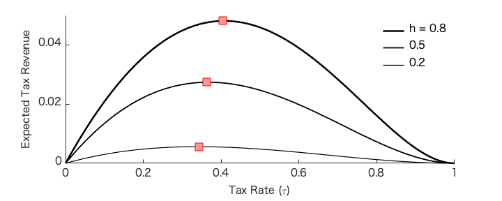
Figure 1: Illustration of tax revenue

Assume, for concreteness, that the authority maximizes the expected tax revenue, which is equal to a $\tau$-fraction of the gross price $(\theta-Y)$ multiplied by the aggregate sales $Y=\int_{0}^{1}X(i){\rm d}i$ in equilibrium. Taking the expectation about $\theta$ and $Y$, we have

$$\operatorname{\mathbb{E}}\quantity[\text{Tax Revenue}]=\tau\operatorname{\mathbb{E}}\quantity[(\theta-Y)\cdot Y] =\tau\operatorname{\mathbb{E}}\quantity[\int_{0}^{1}\quantity(\theta-\int_{0}^{1}X(j){\rm d}j)\cdot X(i){\rm d}i]$$

$$=\tau\int_{0}^{1}\quantity(\operatorname{\mathbb{C}ov}(X(i),\theta)-\int_{0}^{1}\operatorname{\mathbb{C}ov}(X(i),X(j)){\rm d}j){\rm d}i$$

$$=\tau\int_{0}^{1}\operatorname{\mathbb{V}ar}(X(i)){\rm d}i$$

$$=\tau\int_{0}^{1}\varphi(i)^{2}{\rm d}i,$$ (12)

where the third line follows from the obedience condition (9), and the last line holds by Lemma 1. Then, plugging (11) into (12), we have

$$\Pi(\tau;h)=\frac{\tau(1-\tau)^{2}h^{2}}{(1+(1-\tau)h^{2})^{2}}.$$

As displayed in Figure 1, the tax revenue as a function of $\tau$ behaves differently across $h$. In particular, the maximizer of the function depends on how much demand uncertainty the firms face, which means that the authority needs to know the underlying information structure to optimally choose $\tau$.

4 Identification of Information Structures

We now turn to our main focus, investigating the empirical content of Bayesian rational behavior in the LQG framework. This issue will be explored from the perspective of identification in econometrics (Manski, 1995). Suppose that our econometrician has access to the data on equilibrium outcomes, while she does not know precisely the primitives of an LQG game in play. Her objective is to recover the underlying information structure from observables, at least, in a partial sense.

4.1 Data and Hypothesis

Identification hinges crucially on the empirically relevant assumptions about a dataset and a structural model. It becomes more difficult for the econometrician to pin down parameters of interest when available data is weak and only limited hypotheses are made about the structural model. In what follows, we describe layers of such assumptions that we are going to consider.

We begin by describing an assumption about the data that the econometrician observes. Throughout we assume that the econometrician knows, at least, the common state prior, i.e., the fact that $\theta$ is ex-ante normally distributed with mean $\mu_{\theta}$ and variance $\sigma^{2}_{\theta}$. Since our interest lies in identifying the agent’s heterogenous informational traits, we consider the possibility of identification with access to rich individual choice data. The strongest form of such is to assume that the entire joint distribution of the state and actions is observable. In contrast, we also consider weaker forms whose requirement levels differ with the chosen number $T\in\mathbb{N}$.

• (Joint Observability). The econometrician observes the joint distribution of $\mathcal{X}$.

• ($T$-Conditional Observability). The econometrician observes the conditional action distributions $X(\cdot)|_{\theta=\bar{\theta}_{t}}$ for finitely many $T$ distinct values of state realizations $\bar{\theta}_{1},\ldots,\bar{\theta}_{T}\in\mathbb{R}$, which are also observable.

Given that the common state prior is known to the econometrician, the assumption of joint observability essentially postulates that the econometrician can observe the conditional action distribution $X(\cdot)|_{\theta=\bar{\theta}}$ for every state realization $\bar{\theta}\in\mathbb{R}$. This would be quite unrealistic if we interpret each realization of $\theta$ as a counterfactual event and the sampling process is limited. By contrast, under the alternative assumption of $T$-condition observability, the econometrician has access to data on conditional action distributions just for finitely many state realizations.

Next, we set out assumptions imposed on a structural model—called hypotheses—that describe the econometrician’s prior knowledge about the underlying data-generating process. Throughout we shall adopt it as the most fundamental hypothesis that observed data is the result of Bayesian rational agents playing an affine equilibrium of some LQG game, while the econometrician does not have precise knowledge as to which LQG game is in play. Put differently, the econometrician faces a “parametric” identification problem, where the relevant parameters are the primitives of an LQG game. In particular, our interest lies in the identifiability of information structures $\mathcal{P}$.

Table 1: Identification assumptions

	Data	Hypothesis on Payoff St.	Hypothesis on Info. St.
Section 4.2 (Theorem 2)	Joint Obs.	Known	General
Section 4.3 (Theorem 3)	$T$-Cond. Obs.	Unknown	Canonical
Section 4.4.1 (Theorem 4)	$T$-Cond. Obs.	Unknown	Canonical
Section 4.4.2 (Theorem 5)	$T$-Cond. Obs.	Unknown	General

Just like the observability assumptions, several hypotheses of varying strength will be considered in this section. A payoff structure is either completely known or unknown to the econometrician, depending on the nature of the results that we are going to derive. An information structure is unknown to the econometrician, but the set of information structures deemed possible depends on analysis. Specifically, we assume either the underlying information structure can be arbitrarily general or it belongs to what we call the “canonical” class (Definition 5). Table 1 clarifies the identification assumptions that we are going to consider to derive each result.

Example (Continued).

Hereafter, we discuss the example by viewing the tax authority as the econometrician. As we have seen before, the tax revenue depends both on the chosen $\tau$ and the underlying information structure, which is initially unknown. The tax authority has access to rich data on the firms’ past production choices under the initial tax rate, say $\tau_{0}=0$, before changing it to another $\tau$. Our observability assumptions require the observability of the distribution of each individual firm’s choices, by which the availability of a cross-section dataset is presumed.

One way to structure such a dataset is to record the realized values of states and actions for a long period of time. This sort of dataset may be feasible when the identical game is repeated over time but by redrawing shocks on the demand curve and private signals independently across time periods. Another way of interpreting the cross-section dataset is to view each index $i$ as the “type” of firms, rather than an individual firm, and construct the type $i$’s choice distribution in a given period. In this case, $T$-conditional observability requires the repetition of the game just for a short period of time, but instead, there must exist sufficiently many firms belonging to $i$ whose choices are perturbed by purely idiosyncratic noise.

Regarding the econometrician’s hypotheses, it would be natural to assume that the payoff structure is known to the tax authority in the current context. More generally, however, our identification results can also speak about the situation where the tax authority does not know precisely how the demand shock $\theta$ and the aggregate production $Y$ are translated into the market price.

4.2 Canonical Information Structure

In this section, we impose no hypothesis on the class of information structures to be considered. Instead, we assume that the econometrician observes the entire joint distribution of an equilibrium outcome and knows the precise payoff structure $(b,c,w)$.

The next definition offers a class of simple information structures, which is going to be the key throughout all subsequent results.

Definition 5.

An information structure $\mathcal{P}^{*}$ is said to be canonical if every agent receives a uni-dimensional signal, i.e., $\bar{d}=1$, which is generated by the following statistical model: For all $i\in[0,1]$,

$$S^{*}(i)=h(i)\cdot\theta+\varepsilon(i),\quad\operatorname{\mathbb{V}ar}(S^{*}(i))=1,\quad\operatorname{\mathbb{C}ov}(\theta,\varepsilon(i))=0,$$

where $h:[0,1]\to\mathbb{R}$ is a (deterministic) function and $\varepsilon(\cdot)\sim{\rm GP}(0,g)$ is a centered Gaussian process that has a covariance function $g:[0,1]^{2}\to\mathbb{R}$.

There are several special aspects of canonical information structures. First, under a canonical information structure, every agent just receives a uni-dimensional signal $S^{*}(i)\in\mathbb{R}$. Second, the variance is normalized so that $\operatorname{\mathbb{V}ar}(S^{*}(i))=1$. Third, $S^{*}(i)$ is additively decomposable into two parts, that is, the common part—i.e., $h(i)\cdot\theta$—and the idiosyncratic part—i.e., $\epsilon(i)$. Since these are assumed to be uncorrelated, the exposure function $h:[0,1]\to\mathbb{R}$ represents the informativeness of each agent’s signal $S^{*}(i)$ about the state $\theta$. On the other hand, we still allow for the possibility that different agents’ idiosyncratic parts are correlated with one another, and the correlation is captured by the idiosyncratic kernel $g:[0,1]^{2}\to\mathbb{R}$. Any canonical information structure is effectively summarized by the two functions $h$ and $g$. In light of this, we shall refer to the pair $(h,g)$ itself as a canonical information structure.

The next theorem states that given any fixed payoff structure $(b,c,w)$, an arbitrary general information structure $\mathcal{P}$ has an observationally equivalent canonical information structure $\mathcal{P}^{*}$ in the sense of generating the same joint distribution of equilibrium outcomes. As a mnemonic, hereafter, we are going to use superscripts “$*$” with the intention of expressing variables associated with a canonical information structure.

Theorem 2.

Fix any payoff structure $(b,c,w)$. Let $\mathcal{P}$ be an arbitrary information structure, and let $\bar{\varphi}$ be an affine equilibrium in the LQG game $(b,c,w,\mathcal{P})$ such that $\varphi(i)\neq 0$ for all $i\in[0,1]$. Then, there exists a canonical information structure $\mathcal{P}^{*}$ and an affine equilibrium $\bar{\varphi}^{*}$ in the LQG game $(b,c,w,\mathcal{P}^{*})$ such that the induced outcome of $(\mathcal{P}^{*},\bar{\varphi}^{*})$ has the same joint distribution as the induced outcome of $(\mathcal{P},\bar{\varphi})$.

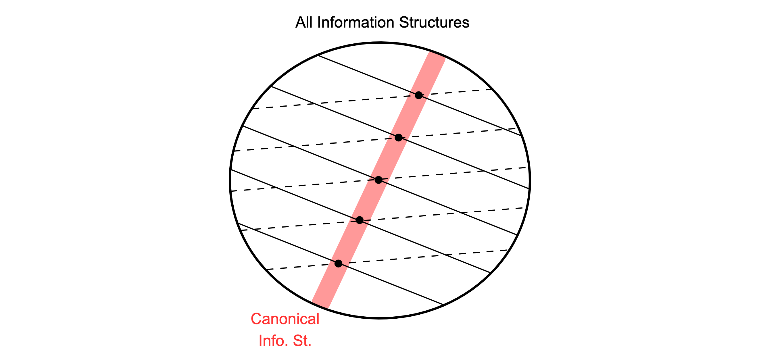
Figure 2: Illustration of Theorem 2

Roughly, Theorem 2 says that, given a fixed payoff structure, the whole set of information structures is divided into observationally equivalent subclasses, each of which has some canonical information structure as the representative element. This is schematically described in Figure 2, where the set of all information structures is divided by observationally equivalent subclasses, which are represented as parallel lines. The way of division depends on the choice of payoff structures, that is, different payoff structures give rise to different collections of parallel lines (solid or dashed). Regardless of the choice of a payoff structure, however, we can always find a canonical information structure as the representative element of each line.

From the modeling perspective, Theorem 2 implies that the modeler incurs no loss of generality to explain any possible equilibrium outcome by assuming as if agents’ signals are generated from some canonical information structure. On the other hand, the theorem points out the limit of the full identification of information structures, even when the strongest data is available to the econometrician if no hypothesis is made as to the class of information structures in consideration. In response to this observation, we thereby seek an affirmative resolution to our identification exercise by hypothesizing that the observed equilibrium outcome is a result of some canonical information structure.

4.3 Identification in the Canonical Class

From now on, we hypothesize that the underlying information structure belongs to the canonical class, and consider the identifiability of the associated exposure function $h$ and idiosyncratic kernel $g$. Note that this canonicality hypothesis may not be regarded as an assumption about the econometrician’s prior knowledge. Rather, it can be interpreted as an as-if assumption made by the econometrician to facilitate the identification exercise. A potential issue is that economic variables identified under the as-if assumption need not reflect the actual variables of interest; this issue will be examined in Section 4.4 in relation to the identifiability of variance reduction.

The next theorem states that the parameters of canonical information structures are identified, at least, up to the magnitude. It turns out that the result only requires the weak forms of assumptions on the data and payoff structures, instead of employing the strong form of hypothesis on information structures. Specifically, joint observability is no longer needed, but rather, we just need conditional action distributions for two distinct state realizations. In addition, the identification can be robustly implemented in the sense that it requires no prior knowledge about the underlying payoff structure.

Theorem 3.

Let $\mathcal{X}$ be an induced outcome of an unknown LQG game $(b,c,w,\mathcal{P}^{*})$, and assume that $\mathcal{P}^{*}$ is canonical and $\operatorname{\mathbb{V}ar}\quantity(X(i))\neq 0$ for all $i\in[0,1]$. Then, under the $2$-conditional observability, $\mathcal{P}^{*}$ is identified in the canonical class up to the absolute values, i.e., any two conditional action distributions $X|_{\theta=\bar{\theta}}$ and $X|_{\theta=\bar{\theta}^{\prime}}$ such that $\bar{\theta}\neq\bar{\theta}^{\prime}$ uniquely pin down the values of $|h(i)|$ and $|g(i,j)|$ for all $i,j\in[0,1]$.

This theorem indicates that identification becomes feasible up to mild qualifications by restricting attention to the canonical class, and in this sense, it proves the canonical class is parsimonious while being able to rationalize all possible equilibrium outcomes. We will illustrate Theorems 2 and 3 in Section 4.5 based on geometric arguments, but the key idea can be roughly explained as follows. The foundation for our identification result lies in the following reduced form expression of equilibrium actions:

$$X(i) =\varphi_{0}^{*}(i)+\varphi_{1}^{*}(i)\cdot S^{*}(i)$$

$$=\varphi_{0}^{*}(i)+\varphi_{1}^{*}(i)h(i)\cdot\theta+\varphi_{1}^{*}(i)\cdot\varepsilon(i),\quad\varepsilon(\cdot)\sim{\rm GP}(0,g),$$ (13)

implied from the definitions of affine strategies and canonical signals. By viewing the equation as the linear regression model, the orthogonality of the state $\theta$ and noise $\epsilon(\cdot)$ leads to the identification of coefficients, $\varphi_{0}^{*}(\cdot)$ and $\varphi_{1}^{*}(\cdot)h(\cdot)$, by regressing actions $X(i)$ by the state realizations. Moreover, the normalization of canonical signals allows the econometrician to separate the exposure function $h(\cdot)$ from the identified cross term $\varphi_{1}^{*}(\cdot)h(\cdot)$, while the value of $h(\cdot)$ is determined only in the absolute sense because of the multiplicative nature of coefficients.

As partly illustrated above, in the intermediate step to prove Theorem 3, we obtain the identification of an affine equilibrium $(\varphi^{*}_{0},\varphi_{1}^{*})$ that arises under the canonical information structure $\mathcal{P}^{*}$ to rationalize the observed distribution of $\mathcal{X}$. The next corollary states that $\varphi_{0}^{*}$ is fully identified, and $\varphi_{1}^{*}$ is identified up to magnitude.

Corollary 1.

Under the same assumptions of Theorem 3, the equilibrium intercept $\varphi_{0}^{*}(i)$, the magnitude of the equilibrium response $|\varphi_{1}^{*}(i)|$, and the cross terms $\varphi_{1}^{*}(i)h(i)$ and $\varphi_{1}^{*}(i)\varphi_{1}^{*}(j)g(i,j)$ are identified for all $i,j\in[0,1]$.

Again, the limitation of identification is that only $|\varphi(i)|$, $|h(i)|$, and $|g(i,j)|$ are identified, but not necessarily their signs. In other words, the econometrician can learn the magnitude of correlations, but the sign may remain ambiguous. This limitation comes from the following sort of attribution problem: The actions of two different agents could be negatively correlated for different reasons, that is, either because their signals are positively correlated but their reactions to signal realizations are opposite, or because their signals are negatively correlated but they react in the same direction.

One way to sharpen identification is to further strengthen the hypothesis on information structures. Let us say that a canonical information structure $(h,g)$ is positive if $h(i)\geq 0$ for all $i\in[0,1]$, i.e., every agent’s signal is positively correlated, at least, with the state. Notice that this definition still permits different agents’ signals to be negatively correlated. Clearly, under this additional hypothesis, the exposure function $h$ is point-identified from Theorem 3. Moreover, by using the cross terms identified in Corollary 1, the econometrician can also point-identify the equilibrium slope $\varphi_{1}^{*}$ and the idiosyncratic kernel $g$. While positivity may be ad-hoc in some cases, it is satisfied in many informational environments considered in the context of LQG games, e.g., Morris and Shin (2002) and Angeletos and Pavan (2007). In particular, the identification analysis of Bergemann and Morris (2013) also presumes the positivity of state-signal correlations that enables the identification of the sign of payoff-relevant parameters.

Example (Continued).

Within the class of information structures (10), Theorem 3 indicates that the econometrician can identify the parameter $h\in[0,1]$ by observing the choice distribution under initial $\tau_{0}$. This allows the authority to “pin down” the tax revenue function in Figure 1, which in turn makes it possible to choose the optimal $\tau^{*}$ in a way to achieve the peak of the function.

The same approach can be used without assuming the symmetry across firms as in (10), but by assuming that an information structure is canonical and positive. Under these hypotheses, as explained above, Theorem 3 and Corollary 1 uniquely pin down the underlying canonical information structure $(h,g)$. Then, since the econometrician as the tax authority can choose $\tau$, she can compute the unique equilibrium slope function as the solution to the equation (7). Moreover, by using the relation (12), the tax revenue after changing the rate to any $\tau$ can be predicted.

4.4 Identification of Variance Reduction

The results in Section 4.3 are subject to two limitations. First, as already mentioned, the econometrician can learn the magnitude of correlations, but the sign may remain ambiguous. Second, identification relies on the as-if assumption that the underlying information structure belongs to the canonical class.

The purpose of this section is to assess the significance of these limitations in the context of identifying the informativeness of individual agents’ signals, as captured by their (state) variance reduction defined by

$$r(N\mid\mathcal{P})\coloneqq\operatorname{\mathbb{V}ar}(\theta)-\operatorname{\mathbb{V}ar}_{N}(\theta)=\sigma^{2}_{\theta}-\operatorname{\mathbb{E}}_{N}\quantity[(\theta-\operatorname{\mathbb{E}}_{N}\quantity[\theta])^{2}],\quad\forall\text{ finite }N\subseteq[0,1].$$ (14)

Here, $\operatorname{\mathbb{E}}_{N}\quantity[\cdot]=\operatorname{\mathbb{E}}[\cdot\mid\{S(i)\}_{i\in N}]$ and $\operatorname{\mathbb{V}ar}_{N}\quantity(\cdot)=\operatorname{\mathbb{V}ar}(\cdot\mid\{S(i)\}_{i\in N})$, respectively, stand for the conditional expectation and variance operators given the set of signals of agents in $N$. The dependence of $r(\cdot\mid\mathcal{P})$ on the information structure $\mathcal{P}$ reflects the fact that agents’ signals are generated from it. A challenge is that $\mathcal{P}$ is not known a priori. We thereby examine the extent to which this value is revealed through equilibrium behavior in the presence of the two limitations mentioned early.

The above-defined variance reduction is a compelling measurement for the informativeness of signals, especially, in the present Gaussian environment since it does not depend on the realization of conditioning events. Moreover, by viewing each agent’s signal as a statistical experiment for the state, the result of Hansen and Torgersen (1974) implies that the informativeness ranking induced by variance reduction coincides with that of Blackwell (1951). Given the strong theoretical foundations for Blackwell’s ranking, this provides a further rationale for us to focus on variance reduction to measure the informativeness of agents’ signals.

4.4.1 Canonical Identification of (Higher-order) Uncertainty

To begin with, we isolate the first limitation of the previous identification results from the second by hypothesizing that signals are generated from an unknown canonical information structure $\mathcal{P}^{*}$. Then, by Theorem 3, the parameters of $\mathcal{P}^{*}$ can be identified up to absolute values. Indeed, absolute values will be enough to identify the variance reduction due to the quadratic nature of the index. That is, the indeterminacy of signs is not a serious problem as far as the econometrician’s aim is to identify the amount of private information as measured by variance reduction.

Identification is not only possible for variance reduction, but also for the amount of any higher-order uncertainty faced by agents. To provide systematic analysis, we shall flip the sign of the index, and instead, look at the amount of first-order uncertainty $R_{1}(N\mid\mathcal{P}^{*})\coloneqq\operatorname{\mathbb{V}ar}_{N}\quantity(\theta)$ as measured by the residual state variance conditional of team $N$’s signals. The notion can be extended to higher-order cases; for general $p\geq 2$, let us define the amount of $p$-th order uncertainty faced by $N_{1}\subseteq[0,1]$ along the path of subsets $N_{2},\ldots,N_{p}\subseteq[0,1]$ to be

$$R_{p}(N_{1};N_{2},\ldots,N_{p}\mid\mathcal{P}^{*})\coloneqq\operatorname{\mathbb{V}ar}_{N_{1}}\quantity(\operatorname{\mathbb{E}}_{N_{2}}\cdots\operatorname{\mathbb{E}}_{N_{p}}\quantity[\theta]).$$

We interpret this quantity as representing the amount of uncertainty that $N_{1}$ faces regarding what $N_{2}$ thinks about $N_{3}$ thinks about […] $N_{p}$ thinks about the state (i.e., the estimate made by $N_{p}$ about $\theta$).

Theorem 4.

Under the same assumptions of Theorem 3, $R_{p}(N_{1};N_{2},\ldots,N_{p}\mid\mathcal{P}^{*})$ is identified for any $p\in\mathbb{N}$ and any finite sequence of finite sets $N_{1},\ldots,N_{p}\subseteq[0,1]$.

4.4.2 Variance Reduction Gap

While Theorem 4 hypothesizes that signals are generated from a canonical information structure $\mathcal{P}^{*}$, the potential issues is that the actual information structure $\mathcal{P}$ could be different yet observationally equivalent to $\mathcal{P}^{*}$. In other words, the amount of uncertainty, identified under the canonicality hypothesis, may not be invariant with respect to the change of information indistinguishable from the outside point of view.

In what follows, we investigate how well $r(\cdot\mid\mathcal{P}^{*})$—i.e., the variance reduction identified in Theorem 4 under the canonicality hypothesis—reflects the actual variance reduction $r(\cdot\mid\mathcal{P})$ when $\mathcal{P}^{*}$ and $\mathcal{P}$ are “observationally equivalent.” To investigate this question, it will be convenient to introduce the formal notions of observational equivalence.

Definition 6.

Two information structures $\mathcal{P}$ and $\mathcal{P}^{*}$ are (weakly) observationally equivalent if there exist payoff structures $(b,c,w)$ and $(b^{*},c^{*},w^{*})$ such that the LQG games $\mathcal{G}=(b,c,w,\mathcal{P})$ and $\mathcal{G}^{*}=(b^{*},c^{*},w^{*},\mathcal{P}^{*})$, respectively, have unique affine equilibria $\bar{\varphi}$ and $\bar{\varphi}^{*}$ for which the induced outcomes of $(\mathcal{G},\bar{\varphi})$ and $(\mathcal{G}^{*},\bar{\varphi}^{*})$ have the same joint distribution.

Notice that the above definition is more permissive than the notion of observational equivalence considered in Theorem 2, because $\mathcal{P}$ and $\mathcal{P}^{*}$ can now be coupled with possibly different payoff structures to induce the same outcome distribution. Adopting this “weak” notion reflects the econometrician’s ignorance not only about an information structure but also a payoff structure. Nevertheless, for two information structures that are just weakly observationally equivalent, we can identify systematic relationships between them as stated in the next theorem.

Theorem 5.

Let $\mathcal{P}$ be an arbitrary information structure, and let $\mathcal{P}^{*}$ be a canonical information structure, and assume that they are observationally equivalent. Then, we have $r(\cdot\mid\mathcal{P})\geq r(\cdot\mid\mathcal{P}^{*})$. Moreover, for any finite set $N=\{i_{1},\ldots,i_{n}\}\subseteq[0,1]$, the equality obtains if and only if there exists a vector ${\bm{\beta}}\in\mathbb{R}^{n}$ such that the actual LQG game and its affine equilibrium $(\mathcal{G},\bar{\varphi})$ satisfies

$${\bm{\Phi}}(N){\bm{\beta}}={\bm{V}}(N)^{\frac{1}{2}}{\bm{K}}(N)^{-1}{\bm{K}}_{\theta}(N),$$ (15)

where ${\bm{\Phi}}(N)\in\mathbb{R}^{\bar{d}n\times n}$ and ${\bm{V}}(N)\in\mathbb{R}^{\bar{d}n\times\bar{d}n}$ are the following block-diagonal matrices:

This theorem delivers two results. The first result is the weak inequality to be generally satisfied between an observationally equivalent pair of information structures. When combined with Theorem 4, this result implies that we can identify the “lower bound” on variance reduction that holds across all information structures $\mathcal{P}$ that are observationally equivalent to the canonical $\mathcal{P}^{*}$. This lower bound describes the amount of information about the state that each subset $N$ of the population collectively possesses, at least.

In general, however, there is a gap between the lower bound and the variance reduction obtained under the actual information structure $\mathcal{P}$. The second result is the necessary and sufficient condition under which the gap disappears. Roughly, the equality condition is satisfied if the team $N$’s equilibrium strategies in the actual LQG game are “proportional” to the vector in the right-hand side of (15) that is determined by the actual information structure. In particular, in the case of a singleton set $N=\{i\}$, the condition can be simplified to

$$\lambda\varphi(i)=P_{\theta}(i),\quad\exists\lambda\in\mathbb{R},$$ (16)

which says that the equilibrium slope $\varphi(i)$ is proportional to the signal-state correlation vector. As such, since $\varphi(i)$ and $P_{\theta}(i)$ are vectors of dimension $\bar{d}$, the proportionality condition is trivially satisfied when $\bar{d}=1$, provided that $\varphi(i)\neq 0$. The same observation extends to a general team $N$.

Corollary 2.

Suppose that the actual information structure $\mathcal{P}$ is uni-dimensional, i.e., $\bar{d}=1$. Then, $r(N\mid\mathcal{P})=r(N\mid\mathcal{P}^{*})$ holds for any finite set $N\subseteq[0,1]$, provided that $\varphi(i)\neq 0$ for all $i\in N$.

This corollary implies that it is exactly the uni-dimensionality of canonical information structures that enables the canonical class to serve as the characterization of the lower bound on the amount of variance reduction, while other structural assumptions placed in Definition 5, such as normalization or decomposability, is not essential to derive this lower-bound property. Also, it should be remarked that the difference between uni- and multi-dimensional information structures hinges on our modeling assumption that each agent takes a uni-dimensional action, whereas her signal could be multi-dimensional. In Section 5, however, we will generalize Corollary 2 to accommodate multi-dimensional actions and show that the variance reduction gap disappears whenever the dimension of an action space is weakly greater than that of a signal space (Proposition 1). Namely, it is the algebraic richness of actions vis-à-vis signals that is crucial to achieving the full identification of variance reduction.

The algebraic richness demands more than the topological richness, which, roughly speaking, requires any action to be arbitrarily well approximated by another action. The latter has been the key for rational behavior to reveal private information in other contexts such as social learning; Lee (1993) demonstrates that with a continuum of actions, each agent’s rational behavior can fully reveal one’s private signal to successors, and the failure of social learning as in Banerjee (1992) and Bikhchandani et al. (1992) will be stripped away. As such, the crucial ingredient of our model is the presence of payoff externalities among agents, which makes agents care not only about the fundamental state but also others’ strategic behavior. As a result, their equilibrium strategies confound both aspects of each agent’s best estimates about the fundamental and strategic uncertainty, which complicated the econometrician’s identification problem.

The substantial role of strategic interactions can be clearly highlighted through the characterization of the equilibrium slope function, that is, the second-moment restriction. Specifically, in the second line of (BNE), notice that the signal-state covariance vector $P_{\theta}(i)$ appears as the second term on the right-hand side, and consequently, the proportionality condition is automatically satisfied for a singleton set $N=\{i\}$ if the first integral term vanishes. This happens, for example, when $w(i,\cdot)$ is constantly equal to zero (among other cases). Hence, the absence of strategic interactions makes it possible for equilibrium actions to fully reveal each agent’s best estimate of the fundamental state. This observation leads us to the next corollary, which together collects other possible cases of when the integral term vanishes.

Corollary 3.

Suppose that a unique affine equilibrium exists in the actual LQG game $\mathcal{G}$ and that $b(i)\neq 0$. Then, $r(i\mid\mathcal{P}^{*})=r(i\mid\mathcal{P})$ holds if either of functions $b(\cdot)$, $w(i,\cdot)$, $P_{\theta}(\cdot)$, or $P(i,\cdot)$ is zero for almost every $j\in[0,1]\setminus\{i\}$.

To illustrate the confounding issue caused by strategic interactions, suppose that the econometrician observes a fairly high correlation between agent $i$’s action $X(i)$ and the state realization $\theta$. The correlation could be attributed to the high predictive accuracy of agent $i$’s signal $S(i)$ about $\theta$, which enables the agent to better adjust her action to the state. Yet, another possibility is that $S(i)$ is just highly predictive about another agent $j$’s signal, as well as $j$’s action, which is in turn highly correlated with the state. In other words, the observed correlation between $X(i)$ and $\theta$ could be just “spurious” as being caused through the combination of $i$’s strategic motive to coordinate with $j$ and $j$’s fundamental motive to well adapt the state. While these two possibilities are hardly distinguished from the outside viewpoint, the combination of our Theorems 4 and 5 indicates that the econometrician can, at least, tightly identify the minimum amount of private information on the state held by agents.

Example (Continued).

The expected tax revenue could be calculated for a counterfactual tax rate $\tau$ under the hypothesis that an information structure is canonical. This would not be the case in general, however, our identification results can be still useful to derive the lower bound on the expected tax revenue by identifying the lower bound on the accuracy of firms’ private information.

To relate an information structure with the tax authority’s objective, we recall that from (12), the expected tax revenue is represented as a $\tau$-fraction of the integration of individual action volatility. The next lemma provides a lower bound on the expected tax revenue for a general information structure $\mathcal{P}$ by deriving the lower bound on individual volatility based on the equilibrium characterization (7).

Lemma 2.

In equilibrium, the following lower bound on the expected tax revenue holds:

$$\operatorname{\mathbb{E}}\quantity[\text{\rm Tax Revenue}]\geq r(\tau)\cdot\int_{0}^{1}P_{\theta}(i)^{\top}P_{\theta}(i){\rm d}i\quad\text{where}\quad r(\tau)=\frac{\tau(1-\tau)^{2}}{2-\tau}.$$ (17)

Now, we observe that $P_{\theta}^{\top}(i)P_{\theta}(i)$ amounts exactly to the variance reduction of firm $i$ under an information structure $\mathcal{P}$, thus its lower bound can be identified through Theorems 4 and 5 to hold across all observationally equivalent information structures. Combining this with (17), we can then obtain the lower bound on the expected tax revenue for any counterfactual rate $\tau$.

4.5 Geometric Illustration

In this section, we explain the logic behind our identification results, Theorems 2–5, by appealing to geometric arguments. To this end, suppose for simplicity that the econometrician has access to the data on the joint distribution of an equilibrium outcome $\mathcal{X}$. Also, assume that every random variable has zero mean. Then, we consider the Hilbert space consisting of all zero-mean and square-integrable random variables defined on the probability space on which the Gaussian process $\mathcal{X}$ is taken place. In Figures 3 and 4, we depict by vectors to schematically express any members of $\mathcal{H}$. Notice that the inner product between any elements of $\mathcal{H}$ is given as their covariance. We assume that $\operatorname{\mathbb{V}ar}(X(i))>0$ for all agents to avoid degenerate cases.

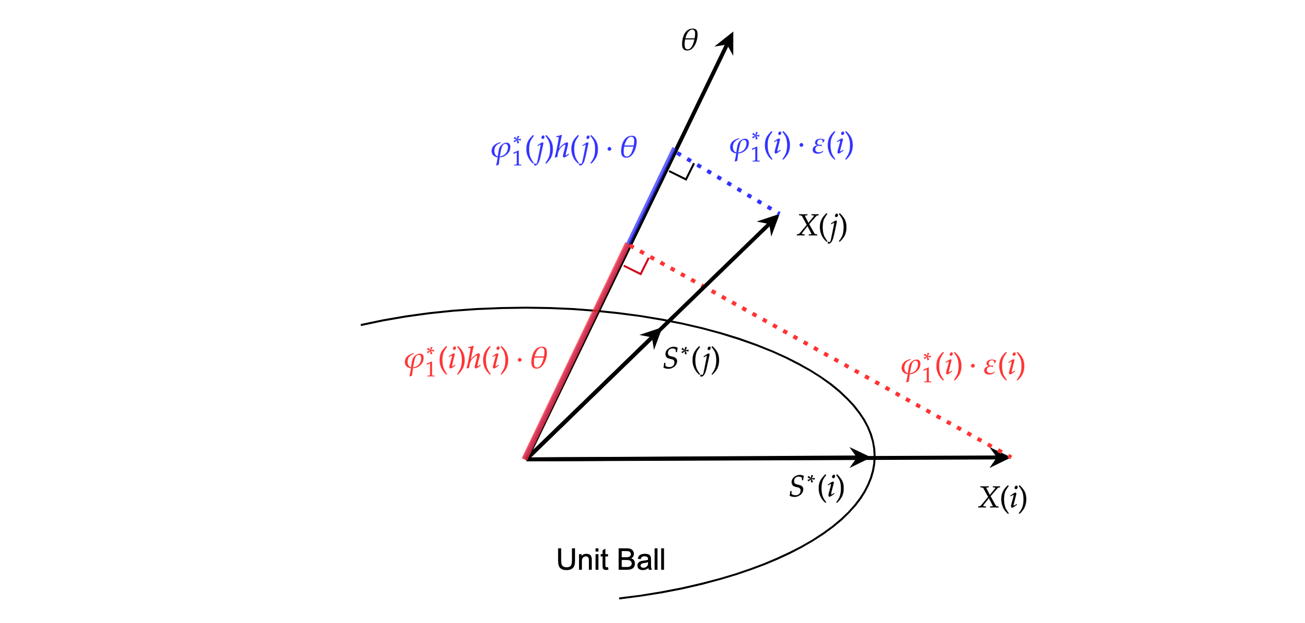
Figure 3: Illustration of a canonical information structure

Constructing a canonical information structure. We first discuss Theorems 2 and 3 together to demonstrate how one can construct a “unique” canonical information structure $(h,g)$ to rationalize the observed equilibrium outcome $\mathcal{X}$. Our point of departure is the reduced form equation (4.3) that should be satisfied by $(h,g)$, together with the associated affine equilibrium $\varphi_{1}^{*}$, to be consistent with the distribution of $\mathcal{X}$ (note that $\varphi_{0}^{*}\equiv 0$ by the zero-mean assumption). To determine the values of these functions, we consider the linear regression of each $X(i)$ on $\theta$. Then, it is a result of the standard projection theorem that there exists a unique function $\psi:[0,1]\to\mathbb{R}$ and a unique process $\eta(\cdot)$ living in the orthogonal complement of the span of $\theta$ such that

$$X(i)=\psi(i)\cdot\theta+\eta(i),\quad\forall i\in[0,1].$$ (18)

Then, matching the coefficients between (4.3) and (18), we can uniquely recover the cross term $\varphi_{1}^{*}(i)h(i)$ by equalizing it to $\psi(i)$. Also, we can recover $\varphi_{1}^{*}(i)\varphi_{1}^{*}(j)g(i,j)$ by equalizing it to the inner product between the residual terms $\eta(i)$ and $\eta(j)$ in the regression (18). In particular, the uniqueness of orthogonal decompositions implies that these cross terms are point-identified, as stated in Corollary 1.

The above regression procedure is illustrated in Figure 3. Here, the actions $X(i)$ and $X(j)$ are orthogonally decomposed into the exposure to the state $\theta$ and the residual, which gives rise to the identification of the cross terms in Corollary 1. In order to determine the canonical information structure $(h,g)$ from $\mathcal{X}$, we still have to extract these functions from the above-identified cross terms. At this point, the normalization of canonical signals—namely, $\operatorname{\mathbb{V}ar}(S^{*}(i))=1$ holds—has a role in providing an additional equation that we can use to recover three unknown functions (i.e., $h$, $g$, $\varphi^{*}_{1}$). Geometrically, this requirement forces each canonical signal $S^{*}_{1}(i)$ to rest on the boundary of the unit ball. Algebraically, it places the parametric requirement on $(h,g)$ by forcing them to satisfy $h(i)^{2}\sigma^{2}_{\theta}+g(i,i)=1$. Combining this equation with the preceding cross terms, we can then pin down the three unknown functions, yet, up to absolute values because of the multiplicative nature of the relevant equations. This provides the rationale for the uniqueness in Theorem 3. Notice that the underlying payoff structure is relevant to determine $\varphi^{*}_{1}$, but identification does not require any knowledge about it, as we directly recover the agents’ reactions to their signals by regressing their observed actions on the state realizations.

There are two remaining things to be verified to justify Theorem 2,. First, the recovered function $g$ should be positive semidefinite to represent the covariance of the Gaussian process. Second, we have to check that $\varphi^{*}_{1}$ constitutes an affine equilibrium under the canonical information structure $(h,g)$. Both can be verified through the distributional properties of $X(\cdot)$, as we will thoroughly discuss in the appendix proof. Especially for the latter, an important observation is going to be that $\mathcal{X}$ is an equilibrium outcome, and hence, its distribution obeys the moment restrictions of the form (8) and (9).

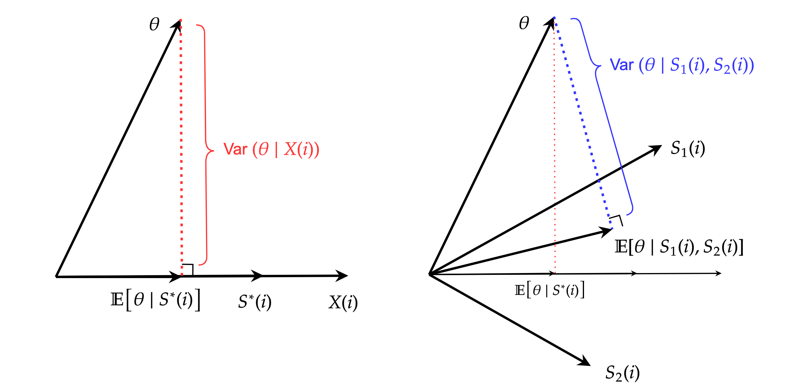
Figure 4: Illustration of a variance reduction gap

Variance reduction gap. Now, let us provide the intuitions for Theorems 4 and 5 by exploiting similar geometric arguments. Our starting point is the observation that the action $X(i)$ is a linear transformation of the canonical signal $S^{*}(i)$. Thus, observing either of them reduces the same amount of the state variance, i.e., we have

$$\operatorname{\mathbb{V}ar}(\theta\mid X(i))=\operatorname{\mathbb{V}ar}(\theta\mid S^{*}(i)).$$ (19)

This is geometrically illustrated in the left panel of Figure 4, where $X(i)$ and $S^{*}(i)$ span the same linear subspace, onto which $\theta$ is orthogonally projected to yield the best estimate about the state conditional on observing $X(i)$, or equivalently, $S^{*}(i)$. Then, the residual variance (19) is measured as the distance between $\theta$ and the span of $X(i)$, which corresponds to the residual in the linear regression of $\theta$ on $X(i)$. More generally, the residual variance $R_{1}(N)$ of any team $N$ can be obtained by calculating the residual in the linear regression of $\theta$ on $\{X(i)\}_{i\in N}$, which provides the rationale for the identifiability of the (first-order) uncertainty in Theorem 4.

Next, to gain the intuition for Theorem 5, let us assume that the actual information structure generates a two-dimensional signal $S(i)=(S_{1}(i),S_{2}(i))$ for each agent. In the right panel of Figure 4, the agent $i$’s best estimate $\operatorname{\mathbb{E}}\quantity[\theta\mid S(i)]$ corresponds to the projection of $\theta$ onto the span of $S_{1}(i)$ and $S_{2}(i)$, whose residual gives rise to the agent $i$’s residual variance $\operatorname{\mathbb{V}ar}(\theta\mid S(i))$. At this point, notice that the action $X(i)$ is a linear transformation of the actual signal $S(i)$, and thus, so must be the canonical signal $S^{*}(i)$. This implies that we necessarily have a more accurate estimate about the state by estimating it from $S(i)$ than from $S^{*}(i)$, which indicates that the weak inequality generally holds. We can geometrically interpret this in the figure by observing that the dashed blue line must be always weakly shorter than the dashed red line. On the other hand, equality is achieved if and only if both $\operatorname{\mathbb{E}}\quantity[\theta\mid S^{*}(i)]$ and $\operatorname{\mathbb{E}}\quantity[\theta\mid S(i)]$ lie on the same linear subspace spanned by $X(i)$. This geometric observation can be algebraically translated to the proportionality condition (15). Notice that the condition is automatically satisfied when $S(i)$ is uni-dimensional since, in that case, all of $S(i)$, $S^{*}(i)$, and $X(i)$ must be parallel to each other.

On the other hand, when $S(i)$ is multi-dimensional, the condition is generically violated, except on the knife edge, and there generally arises a gap between $r(i\mid\mathcal{P}^{*})$ and $r(i\mid\mathcal{P})$. Specifically, the gap can be quantified by the geometric measure of (squared) cosine similarity as follows:

$$\frac{r(i\mid\mathcal{P}^{*})}{r(i\mid\mathcal{P})}=\cos^{2}(\varphi(i),P_{\theta}(i)).$$ (20)

Here, $\cos\quantity(v,v^{\prime})$ denotes the cosine of the angle between vectors $v,v^{\prime}\in\mathbb{R}^{\bar{d}}$, which is known as a measurement of the proximity between two vectors. The fact that the ratio is expressed as the “squared” cosine similarity means that the variance reduction gap gets small when the agent’s equilibrium response $\varphi(i)$ and the signal-state correlations $P_{\theta}(i)$ are close to each other in terms of the minor angle spanned by them. In particular, the gap becomes minimal (resp. maximal) when the two vectors are parallel (resp. orthogonal).

5 Extensions

So far, we have imposed several modeling assumptions, either implicitly or explicitly, to facilitate our analysis and notation. Some of them can be relaxed to further generalize our findings. This section discusses some possible extensions.

5.1 Idiosyncratic Payoff Shock

Several preceding papers admit the heterogeneity across agents in terms of payoff-relevant states (Bergemann et al., 2015, 2017a, Lambert et al., 2018a). That is, there are as many states $\theta(i)$ as the number of agents, and each state is relevant just to the corresponding agent’s payoff. For example, Bergemann et al. (2015) model the heterogeneous payoff shocks by letting $\theta(i)=\theta+\Delta\theta(i)$, where the base state $\theta$ is perturbed by i.i.d. Gaussian noise $\Delta\theta(i)$. In the present framework, we can incorporate general payoff shocks by extending the primitive collection of random variables to

$$\mathcal{S}=\quantity{\theta(i),S_{1}(i),\ldots,S_{\bar{d}}(i)}_{i\in[0,1]}.$$

Let us continue to assume that the above-defined $\mathcal{S}$ is Gaussian, i.e., any finitely many picks from $\mathcal{S}$ follows a multivariate normal distribution.

We note, however, that this change brings about no essential change in any of our analysis due to the flexibility of our baseline model. Indeed, repeating the same arguments that derive (BNE), one can show that an affine strategy profile $\bar{\varphi}$ constitutes a Bayesian Nash equilibrium under the present setup if and only if $\bar{\varphi}$ solves the following Fredholm equation:

$$\matrixquantity[\varphi_{0}(i)\\ \varphi(i)]=\matrixquantity[\displaystyle\int_{0}^{1}w(i,j)\varphi_{0}(j){\rm d}j\\ \displaystyle\int_{0}^{1}w(i,j)P(i,j)\varphi(j){\rm d}j]+\underbrace{\matrixquantity[\mu_{\theta}(i)b(i)+c(i)\\ \sigma_{\theta}(i)b(i)\tilde{P}_{\theta}(i)]}_{\eqqcolon\ f(i)},\quad\forall i\in[0,1].$$

Here, $\mu_{\theta}(i)\coloneqq\operatorname{\mathbb{E}}\quantity[\theta(i)]$, $\sigma_{\theta}(i)\coloneqq\sqrt{\operatorname{\mathbb{V}ar}\quantity(\theta(i))}$, $\tilde{P}_{\theta}(i)\coloneqq\frac{1}{\sigma_{\theta}(i)}\operatorname{\mathbb{V}ar}\quantity(S(i))^{-\frac{1}{2}}\operatorname{\mathbb{C}ov}\quantity(S(i),\theta(i))$, and all other terms are the same as before. Importantly, payoff shocks affect only the constant term $f(\cdot)$ in regard with $\bar{\varphi}$, but they do not affect the integrands. As a result, the above equation has a unique solution if and only if $w$ and $P$ are such that the original equation (BNE) has a unique solution. Moreover, when all $\theta(i)$ are i.i.d. perturbations of the common state $\theta$ as in Bergemann et al. (2015), any noise added to $\theta$ is irrelevant for the analyst’s inference problem about $\theta$. Hence, all the previous results are kept the same verbatim.

5.2 Multi-dimensional Action

As the geometric arguments in Section 4.5 suggests, the key to obtain the variance reduction inequality $r(\cdot\mid\mathcal{P}^{*})\leq r(\cdot\mid\mathcal{P})$ is to intermediate it by the amount of the state variance reduced by observing the action (whose distribution is the same under $\mathcal{P}$ and $\mathcal{P}^{*}$). That is, we consider the index of variance reduction defined for actions such that

$$\hat{r}(N\mid\mathcal{P},\varphi)\coloneqq\sigma^{2}_{\theta}-\operatorname{\mathbb{V}ar}\quantity(\theta\mid\{X(i)\}_{i\in N}),\quad\forall\text{ finite }N\subseteq[0,1],$$ (21)

where $X(i)=\varphi_{0}(i)+\varphi(i)^{\top}K(i,i)^{-\frac{1}{2}}\quantity(S(i)-m(i))$ is an affine strategy defined based on $\bar{\varphi}\in\mathcal{L}_{2}[0,1]$. Then, the proof of Theorem 5 reveals that $\hat{r}(\cdot\mid\mathcal{P},\varphi)$ is, in general, weakly less than $r(\cdot\mid\mathcal{P})$, while the equality obtains if $\mathcal{P}$ is uni-dimensional. At this point, what makes the uni-dimensional information structures special is the uni-dimensionality of actions, which our model has maintained so far. As we show below, however, a similar observation extends to incorporating multi-dimensional actions. This extension highlights the importance of the relative dimension of actions vis-à-vis signals for the point-identification of state variance reduction.

We now consider the situation where each agent $i$ takes a multi-dimensional action $x(i)\in\mathbb{R}^{\bar{d}_{\rm x}}$ upon receiving a multi-dimensional signal $s(i)\in\mathbb{R}^{\bar{d}_{\rm s}}$, where $\bar{d}_{\rm x},\bar{d}_{\rm s}\in\mathbb{N}$. An affine strategy in this setting is described as

$$X(i)=\varphi_{0}(i)+\Phi(i)^{\top}\underbrace{K(i,i)^{-\frac{1}{2}}\quantity(S(i)-m(i))}_{\text{Standardized signal}},$$

where the intercept $\varphi_{0}(i)\in\mathbb{R}^{\bar{d}_{\rm x}}$ is a constant vector, and the slope $\Phi(i)\in\mathbb{R}^{\bar{d}_{\rm s}\times\bar{d}_{\rm x}}$ is a constant matrix such that the $d$-th column describes how the agent $i$’s $d$-th action is determined responding to her standardized signal. Ignoring the intercept, as it is irrelevant to computing variance reduction, an affine strategy profile would then be identified with a matrix-valued function $\Phi:[0,1]\to\mathbb{R}^{\bar{d}_{\rm s}\times\bar{d}_{\rm x}}$ such that every argument belongs to $\mathcal{L}_{2}[0,1]$. Then, for any information structure $\mathcal{P}$ the index $\hat{r}(N\mid\mathcal{P},\Phi)$ is defined analogously to (21) for each team $N\subseteq[0,1]$, as the amount of state variance reduced by observing $\bar{d}_{\rm x}$-dimensional actions of the agents in $N$.

The next proposition reveals that $r(\cdot\mid\mathcal{P},\Phi)$ is weakly less than $r(\cdot\mid\mathcal{P})$, while the equality obtains if actions are rich enough to span multi-dimensional signals.

Proposition 1.

For any information structure $\mathcal{P}$ and affine strategy profile $\Phi$, we have $r(\cdot\mid\mathcal{P})\geq\hat{r}(\cdot\mid\mathcal{P},\Phi)$. Moreover, for any finite set $N=\{i_{1},\ldots,i_{n}\}\subseteq[0,1]$, the equality $r(N\mid\mathcal{P})=\hat{r}(N\mid\mathcal{P},\Phi)$ obtains if and only if there exists a vector ${\bm{\beta}}\in\mathbb{R}^{n\bar{d}_{\rm x}}$ satisfying (15), where the matrix ${\bm{\Phi}}(N)$ is now defined as

In particular, the equality condition holds if ${\bm{\Phi}}(N)$ has full row rank.

According to Proposition 1, the observer can reduce the state variance by observing multi-dimensional actions as much as she could do by directly observing multi-dimensional signals if and only if the proportionality condition (15) holds. Importantly, the condition is automatically satisfied when ${\bm{\Phi}}(N)$ has full row rank, or equivalently, so does $\Phi(i)$ for every $i\in N$. As such, when $\bar{d}_{\rm x}=\bar{d}_{\rm s}=1$, the full rankedness is just saying that $\varphi(i)$ is non-zero, which is generically satisfied. In general, that $\bar{d}_{\rm x}\geq\bar{d}_{\rm s}$ is necessary for $\Phi(i)$ to have row full rank, and conversely, it is “almost” sufficient as well, since generic matrices in $\mathbb{R}^{d\times d^{\prime}}$ have rank $\min\{d,d^{\prime}\}$. Therefore, our result suggests that the richness of actions, relative to signals, in terms of dimensionality is important to achieve the zero variance reduction gap between those statistical experiments.

6 Conclusion

This paper studies the identification of an information structure from the distribution of equilibrium actions in a game of incomplete information played by a continuum of agents. To this end, we offer a canonical class of information structures and show that the class is sufficient to rationalize any equilibrium outcome, yet, parsimonious to admit sharp identification results. Moreover, it is shown that a canonical information structure characterizes the minimal amount of private information on the fundamental state that each agent possesses, across all observationally equivalent information structures, as measured in terms of state variance reduction. The lower bound is tight when there are no strategic interactions among agents, but in general, there is a strict gap, because agents’ strategic motives confound their private information about fundamental and strategic uncertainty.

Appendix A Omitted Proofs

In this Appendix A, we provide all proofs omitted from the main text. We start by summarizing the notation that we are going to use, especially, in the proof of Theorem 1. All mathematical definitions are standard and can be found in Lax (2002), Brezis (2010), or Kress (2014), which are the main sources of the functional analysis tools that we are going to utilize.

A.1 Mathematical Preliminaries

We denote by $\mathbb{R}^{n}$ the space of $n$-dimensional (column) vectors and by $\mathbb{R}^{n\times n}$ the space of $(n\times n)$-matrices. We adopt the Euclidean norm on $\mathbb{R}^{n}$ denoted by $\|v\|\coloneqq\sqrt{v^{\top}v}$. The induced operator norm on $\mathbb{R}^{n\times n}$ is denoted by ${\left|\kern-1.07639pt\left|\kern-1.07639pt\left|M\right|\kern-1.07639pt\right|\kern-1.07639pt\right|}\coloneqq\sup_{v\in\mathbb{R}^{n}\setminus\{0\}}\frac{\|Mv\|}{\|v\|}$.

For $n,m\in\mathbb{N}$ and a compact set $A\subseteq\mathbb{R}^{m}$, we denote by $\mathcal{L}_{2}^{n}(A)$ the Hilbert space of vector-valued functions $f,g:A\to\mathbb{R}^{n}$, equipped with the inner product

$$\langle f,g\rangle\coloneqq\int_{A}f(x)^{\top}g(x){\rm d}x,$$

and denote the induced norm by $\|f\|\coloneqq\sqrt{\langle f,f\rangle}$. Note that $\|f\|=(\int_{A}\|f(x)\|^{2}{\rm d}x)^{\frac{1}{2}}$. Extending this definition for a matrix-valued function $F:A\to\mathbb{R}^{n\times n}$, we define its norm by $\|F\|\coloneqq(\int_{A}{\left|\kern-1.07639pt\left|\kern-1.07639pt\left|F(x)\right|\kern-1.07639pt\right|\kern-1.07639pt\right|}^{2}{\rm d}x)^{\frac{1}{2}}$. For a linear operator $T:\mathcal{L}_{2}^{n}(A)\to\mathcal{L}_{2}^{n}(A)$, we denote the induced operator norm by ${\left|\kern-1.07639pt\left|\kern-1.07639pt\left|T\right|\kern-1.07639pt\right|\kern-1.07639pt\right|}\coloneqq\sup_{\|f\|>0}\frac{\|Tf\|}{\|f\|}$. Let $\Lambda(T)$ denote the set of real eigenvalues of $T$. An identify operator is usually denoted by $I$.

In accordance with the above notation, the norm for a payoff structure is given by

$$\|b\|=\quantity(\int_{0}^{1}|b(i)|^{2}{\rm d}i)^{\frac{1}{2}},\quad\|c\|=\quantity(\int_{0}^{1}|c(i)|^{2}{\rm d}i)^{\frac{1}{2}},\quad\|w\|=\quantity(\int_{0}^{1}\int_{0}^{1}|w(i,j)|^{2}{\rm d}j{\rm d}i)^{\frac{1}{2}},$$

and all of which are assumed to be finite as mentioned in Section 2.1. Also, the norm for an information structure is given by

$$\|P\|=\quantity(\int_{0}^{1}\int_{0}^{1}{\left|\kern-1.07639pt\left|\kern-1.07639pt\left|P(i,j)\right|\kern-1.07639pt\right|\kern-1.07639pt\right|}^{2}{\rm d}j{\rm d}i)^{\frac{1}{2}}\quad\text{and}\quad\|P_{\theta}\|=\quantity(\int_{0}^{1}\|P_{\theta}(i)\|^{2}{\rm d}i)^{\frac{1}{2}}$$

Putting these together, we measure the distance between two LQG games having the same dimensionality $\bar{d}$ based on

$$\left\|\mathcal{G}-\mathcal{G}^{\prime}\right\|\coloneqq \left\|b-b^{\prime}\right\|+\left\|c-c^{\prime}\right\|+\left\|w-w^{\prime}\right\|+\left\|P-P^{\prime}\right\|+\left\|P_{\theta}-P^{\prime}_{\theta}\right\|.$$ (A.1)

In Theorem 1, the convergence of LQG games occurs with respect to the norm (A.1), and genericity is meant by the corresponding norm-openness and norm-denseness. With this formalization at hand, we can now formally state Theorem 1; the next restatement slightly strengthens the “denseness” of the unique existence of an affine equilibrium so that the perturbation is given only to the payoff weight function $w$.

Theorem 1 (Restatement).

The following statements hold:

• (Denseness). For every LQG game $\mathcal{G}=(b,c,w,\mathcal{P})$ that does not have a unique affine equilibrium and every $\epsilon>0$, there exists a payoff weight function $w^{\prime}$ with $\|w-w^{\prime}\|<\epsilon$ such that the LQG game $\mathcal{G}^{\prime}=(b,c,w^{\prime},\mathcal{P})$ has a unique affine equilibrium.

• (Openness and Convergence). For every LQG game $\mathcal{G}$ that has a unique affine equilibrium $\bar{\varphi}$, if $\{\mathcal{G}_{n}\}_{n\in\mathbb{N}}$ is a sequence of LQG games such that $\lim_{n\to\infty}\|\mathcal{G}-\mathcal{G}_{n}\|=0$, then $\mathcal{G}_{n}$ has a unique affine equilibrium $\bar{\varphi}_{n}$ for every large $n\in\mathbb{N}$. Moreover, $\lim_{n\to\infty}\|\bar{\varphi}-\bar{\varphi}_{n}\|=0$.

A.2 Proof of Theorem 1

According to Lemma 1, the space of affine strategy profiles can be identified with the Hilbert space $\mathcal{L}_{2}^{\bar{d}+1}[0,1]$. Then, the next lemma indicates that any “regular” strategy profile—defines as per Definition 1—is Pettis integrable and admits a Fubini-like formula (A.2), justifying the interchange of integration and conditional expectation. The proof of this lemma can be found as Corollary 1 and Corollary 2 of Miyashita and Ui (2024).

Lemma A.1.

For any strategy profile $X(\cdot)$ and $i\in[0,1]$, the local aggregate $Y(i)=\int_{0}^{1}w(i,j)X(j){\rm d}j$ exists as the Pettis integral. Moreover, we have

$$\operatorname{\mathbb{E}}_{i}\quantity[Y(i)]=\int_{0}^{1}w(i,j)\operatorname{\mathbb{E}}_{i}\quantity[X(j)]{\rm d}j\quad\forall i\in[0,1].$$ (A.2)

Coupled with Lemma A.1, the preceding discussion following Theorem 1 shows that $\bar{\varphi}\in\mathcal{L}_{2}^{\bar{d}+1}[0,1]$ constitutes an affine equilibrium if and only if it solves the Fredholm equation (BNE). It will be convenient to rewrite the equation as

$$(I-T)(\bar{\varphi})=f,$$ (A.3)

where $T$ is a linear operator acting on $\mathcal{L}^{\bar{d}+1}[0,1]$ such that

and $f$ is a function on $[0,1]$ such that

$$f(\cdot)=\matrixquantity[\mu_{\theta}b(\cdot)+c(\cdot)\\ \sigma_{\theta}b(\cdot)P_{\theta}(\cdot)]\in\mathbb{R}^{\bar{d}+1}.$$ (A.4)

Roughly, (A.3) indicates that a unique affine equilibrium $\bar{\varphi}$ exists when the operator $I-T$ is “invertible,” and this idea is going to be formalized by the Fredholm alternative. To this end, we shall establish a couple of lemmas pertaining to some basic properties of the variables in the equation.

Lemma A.2.

$f\in\mathcal{L}_{2}^{\bar{d}+1}[0,1]$.

Proof.

By the definition of $f$, we have

$$\|f\|^{2}=\|\mu_{\theta}b+c\|^{2}+\sigma_{\theta}^{2}\int_{0}^{1}b(i)^{2}P_{\theta}(i)^{\top}P_{\theta}(i){\rm d}i,$$ (A.5)

whereas $\|\mu_{\theta}b+c\|^{2}<\infty$ because $b,c\in\mathcal{L}_{2}[0,1]$ by assumption. Moreover, since the matrices $K(i,i)$ and

$$\matrixquantity[K(i,i)&K_{\theta}(i)\\ K_{\theta}(i)^{\top}&\sigma^{2}_{\theta}]$$

are positive semidefinite, the Schur complement must be non-negative, i.e., we have $\sigma_{\theta}^{2}-K_{\theta}(i)^{\top}K(i,i)^{-1}K_{\theta}(i)\geq 0$ for every $i\in[0,1]$. Hence, together with the definition of $P_{\theta}(i)$, it follows that

$$\sup_{i\in[0,1]}P_{\theta}(i)^{\top}P_{\theta}(i)=\sup_{i\in[0,1]}\frac{1}{\sigma^{2}_{\theta}}K_{\theta}(i)^{\top}K(i,i)^{-1}K_{\theta}(i)\leq 1.$$ (A.6)

By this and $b\in\mathcal{L}_{2}[0,1]$, we see that the second term of (A.5) is finite, from which $f\in\mathcal{L}_{2}^{\bar{d}+1}[0,1]$ is confirmed. ∎

Lemma A.3.

$\|\bar{P}(i,j)\bar{\varphi}(j)\|\leq\|\bar{\varphi}(j)\|$ for all $\bar{\varphi}\in\mathcal{L}_{2}^{\bar{d}+1}[0,1]$ and $i,j\in[0,1]$.

Proof.

The construction of $\bar{P}(i,j)$ implies $\|\bar{P}(i,j)\bar{\varphi}(j)\|^{2}=|\varphi_{0}(j)|^{2}+\|P(i,j)\varphi(j)\|^{2}$. As such, if $\|P(i,j)\varphi(j)\|^{2}\leq\|\varphi(j)\|^{2}$ holds, then we have

$$\|\bar{P}(i,j)\bar{\varphi}(j)\|^{2}\leq|\varphi_{0}(j)|^{2}+\|\varphi(j)\|^{2}=\|\bar{\varphi}(j)\|^{2},$$

from which the desired inequality obtains. Hence, it is enough for us to show that $\|P(i,j)\varphi(j)\|\leq\|\varphi(j)\|$ holds.

It is a well-known fact in linear algebra that the induced matrix norm of Euclidean coincides with the largest singular value of a matrix (see, e.g., pp. 346 of Horn and Johnson, 2012). Let us denote by $\sigma_{ij}$ the singular value of $P(i,j)$ and by $\lambda_{\rm max}(M)$ the largest eigenvalue of any matrix $M$. By definition, it follows that

$$\sigma_{ij} =\sqrt{\lambda_{\max}\bigl{(}P(i,j)^{\top}P(i,j)\bigr{)}}$$

$$=\sqrt{\lambda_{\max}\bigl{(}K(j,j)^{-\frac{1}{2}}K(j,i)K(i,i)^{-1}K(i,j)K(j,j)^{-\frac{1}{2}}\bigr{)}}$$

$$=\sqrt{\lambda_{\max}\bigl{(}K(j,j)^{-1}K(j,i)K(i,i)^{-1}K(i,j)\bigr{)}},$$ (A.7)

where the last equality comes from the fact that similar matrices have the same set of eigenvalues. Moreover, by the matrix-valued Cauchy–Schwarz inequality in Tripathi (1999), we know that the matrix $K(j,j)-K(j,i)K(i,i)^{-1}K(i,j)$ is positive semidefinite, whence Theorem 7.7.3 (a) of Horn and Johnson (2012) implies

$$\lambda_{\rm max}(K(j,j)^{-1}K(j,i)K(i,i)^{-1}K(i,j))\leq 1.$$ (A.8)

By (A.7) and (A.8), we have $\sigma_{ij}\leq 1$, from which the definition of the matrix norm yields $\|P(i,j)\varphi(j)\|\leq\sigma_{ij}\|\varphi(j)\|\leq\|\varphi(j)\|$, as required. ∎

Lemma A.4.

$T:\mathcal{L}_{2}^{\bar{d}+1}[0,1]\to\mathcal{L}_{2}^{\bar{d}+1}[0,1]$ is a bounded linear operator with ${\left|\kern-1.07639pt\left|\kern-1.07639pt\left|T\right|\kern-1.07639pt\right|\kern-1.07639pt\right|}\leq\|w\|$.

Proof.

It is clear that $T$ acting on $\mathcal{L}_{2}^{\bar{d}+1}[0,1]$ is linear. For boundedness, take any $\bar{\varphi}\in\mathcal{L}_{2}[0,1]$. Given any $i\in[0,1]$, observe that

$$\|T\bar{\varphi}(i)\| \leq\int_{0}^{1}|w(i,j)|\cdot\|\bar{P}(i,j)\bar{\varphi}(j)\|{\rm d}j\leq\int_{0}^{1}|w(i,j)|\cdot\|\bar{\varphi}(j)\|{\rm d}j$$

$$\leq\quantity(\int_{0}^{1}|w(i,j)|^{2}{\rm d}j)^{\frac{1}{2}}\cdot\quantity(\int_{0}^{1}\|\bar{\varphi}(j)\|^{2}{\rm d}j)^{\frac{1}{2}}=\quantity(\int_{0}^{1}|w(i,j)|^{2}{\rm d}j)^{\frac{1}{2}}\cdot\|\bar{\varphi}\|,$$ (A.9)

where the first inequality follows from the convexity of the Euclidean norm and Jensen’s inequality, the second from Lemma A.3, and the third from the Cauchy–Schwartz inequality. Then, squaring both sides and integrating over $i\in[0,1]$, it follows that

$$\|T\bar{\varphi}\|^{2}=\int_{0}^{1}\|T\bar{\varphi}(i)\|^{2}{\rm d}i\leq\quantity(\int_{0}^{1}\int_{0}^{1}|w(i,j)|^{2}{\rm d}j{\rm d}i)\cdot\|\bar{\varphi}\|^{2}=\|w\|^{2}\cdot\|\bar{\varphi}\|^{2},$$

from which $\|T\bar{\varphi}\|\leq\|w\|\cdot\|\bar{\varphi}\|$ holds. Since $\bar{\varphi}$ is arbitrary, we conclude that ${\left|\kern-1.07639pt\left|\kern-1.07639pt\left|T\right|\kern-1.07639pt\right|\kern-1.07639pt\right|}\leq\|w\|$. ∎

The next key lemma strengthens the conclusion of Lemma A.4. On top of being bounded, the operator $T$ is “compact,” i.e., it maps any bounded sequence in $\mathcal{L}_{2}^{\bar{d}+1}[0,1]$ to a pre-compact set in $\mathcal{L}_{2}[0,1]$. Since its verification involves some additional notations, which are mostly orthogonal to the main course of the discussion, we relegate the proof of Lemma A.5 to Appendix A.9.

Lemma A.5.

$T:\mathcal{L}_{2}^{\bar{d}+1}[0,1]\to\mathcal{L}_{2}^{\bar{d}+1}[0,1]$ is a compact linear operator.

Having established that $T$ is a compact operator acting on the Hilbert space $\mathcal{L}_{2}^{\bar{d}+1}[0,1]$, it is a consequence of the Fredholm alternative (see, e.g., Theorem 3.4 of Kress, 2014) that the equation (A.3) has a unique solution $\bar{\varphi}$ in $\mathcal{L}_{2}^{\bar{d}+1}[0,1]$ if and only if the operator $I-T$ is injective. On the other hand, $I-T$ is injective if and only if there exists no non-zero element $\bar{\psi}\in\mathcal{L}_{2}^{\bar{d}+1}[0,1]$ such that $\bar{\psi}=T\bar{\psi}$, which is equivalent to saying that $1$ is not an eigenvalue of $T$. These observations lead us to the next lemma; there, we write $T_{w,\mathcal{P}}$ instead of $T$ in order to emphasize the dependency on primitives.

Lemma A.6.

An LQG game $\mathcal{G}=(b,c,w,\mathcal{P})$ has a unique affine equilibrium if and only if $I-T$ has a bounded inverse, which is further equivalent to the condition $1\notin\Lambda(T_{w,\mathcal{P}})$.

Any compact operator has the important property of having no accumulation point in the set of eigenvalues, possibly, except $0$ (see, e.g., Theorem 3.9 of Kress, 2014). Hence, if $1\in\Lambda(T_{w,\mathcal{P}})$, then we can take $\delta>0$ such that $[1,1+\delta]\cap\Lambda(T_{w,\mathcal{P}})=\{1\}$. Given any small $\epsilon>0$, multiplying both sides by $(1-\epsilon)$ gives rise to

$$\quantity[1-\epsilon,\,(1-\epsilon)(1+\delta)]\cap(1-\epsilon)\Lambda(T_{w,\mathcal{P}})=\{1-\epsilon\},$$

while the construction of $T_{w,\mathcal{P}}$ and the homogeneity of eigenvalues imply

$$(1-\epsilon)\Lambda\quantity(T_{w,\mathcal{P}})=\Lambda\quantity((1-\epsilon)T_{w,\mathcal{P}})=\Lambda(T_{(1-\epsilon)w,\mathcal{P}}).$$

Note that we have $1\in\quantity[1-\epsilon,\,(1-\epsilon)(1+\delta)]$, provided that $\epsilon$ is small enough so that $\epsilon\leq\delta/(1+\delta)$. Thus, the LQG game $\mathcal{G}_{\epsilon}$ obtained from $\mathcal{G}$ by only replacing $w$ by $(1-\epsilon)w$ has a unique affine equilibrium whenever $\epsilon\in(0,\delta/(1+\delta)]$. In particular, the distance between $\mathcal{G}$ and $\mathcal{G}_{\epsilon}$ can be arbitrarily small, from which we confirm that unique existence is a “dense” property.

Next, we shall show that unique existence is an “open” property. To this end, consider any convergent sequence of LQG games $\mathcal{G}_{n}=(b_{n},c_{n},w_{n},\mathcal{P}_{n})$ to the limit LQG game $\mathcal{G}=(b,c,w,\mathcal{P})$, and assume that $\mathcal{G}$ has a unique affine equilibrium. Let $T_{n}$ and $f_{n}$ be defined as in (A.2) and (A.4) but by using the primitives of $\mathcal{G}_{n}$. Also, we use the notations $T$ and $f$ for those associated with $\mathcal{G}$. By Lemma A.6, we have $1\notin\Lambda(T)$.

Lemma A.7.

$\|f-f_{n}\|\to 0$ and ${\left|\kern-1.07639pt\left|\kern-1.07639pt\left|T-T_{n}\right|\kern-1.07639pt\right|\kern-1.07639pt\right|}\to 0$ as $n\to\infty$.

Proof.

We first show that $b_{n}P_{\theta,n}:[0,1]\to\mathbb{R}^{\bar{d}}$ converges to $bP:[0,1]\to\mathbb{R}^{\bar{d}}$ in $L_{2}$. Note that all of these functions belong to $\mathcal{L}_{2}^{\bar{d}}[0,1]$ by Lemma A.2. Then, by the triangle inequality, we have

$$\|bP-b_{n}P_{n}\|\leq\|b(P_{\theta}-P_{\theta,n})\|+\|(b-b_{n})P_{\theta,n}\|.$$

Here, (A.6) implies that the second term is bounded by $\|b-b_{n}\|$, which converges to $0$ as $n\to\infty$. Moreover, (A.6) implies that the function $i\mapsto\|b(i)(P_{\theta}(i)-P_{\theta,n}(i))\|$ is uniformly bounded by the integrable function $i\mapsto 2|b(i)|^{2}$, whence the dominated convergence theorem yields

$$\lim_{n\to\infty}\|b(P_{\theta}-P_{\theta,n})\|^{2}=\int_{0}^{1}|b(i)|^{2}\cdot\quantity(\lim_{n\to\infty}\|P_{\theta}(i)-P_{\theta,n}(i)\|^{2}){\rm d}i,$$

from which we confirm that $\|bP-b_{n}P_{n}\|\to 0$ as $n\to\infty$. Now, by the definition of the norm on $\mathcal{L}_{2}^{\bar{d}+1}[0,1]$, we have

$$\|f-f_{n}\|^{2}=\|\mu_{\theta}(b-b_{n})+(c-c_{n})\|^{2}+\sigma^{2}_{\theta}\|bP_{\theta}-b_{n}P_{\theta,n}\|,$$

which converges to $0$ since $b_{n}\to b$ and $c_{n}\to c$ in $L_{2}$.

To show that ${\left|\kern-1.07639pt\left|\kern-1.07639pt\left|T-T_{n}\right|\kern-1.07639pt\right|\kern-1.07639pt\right|}\to 0$, take any $\bar{\varphi}\in\mathcal{L}_{2}^{\bar{d}+1}[0,1]$. Given any $i\in[0,1]$, one can conduct similar calculations to (A.9) to get

$$\left\|(T-T_{n})(\bar{\varphi})[i]\right\|\leq\quantity(\int_{0}^{1}{\bigl{|}\kern-1.07639pt\bigl{|}\kern-1.07639pt\bigl{|}w(i,j)\bar{P}(i,j)-w_{n}(i,j)\bar{P}_{n}(i,j)\bigr{|}\kern-1.07639pt\bigr{|}\kern-1.07639pt\bigr{|}}{\rm d}j)^{\frac{1}{2}}\cdot\|\bar{\varphi}\|.$$

Since $\bar{\varphi}$ is arbitrary, squaring both sides and integrating over $i\in[0,1]$, we obtain the following upper bound for the operator norm:

$${\left|\kern-1.07639pt\left|\kern-1.07639pt\left|T-T_{n}\right|\kern-1.07639pt\right|\kern-1.07639pt\right|}^{2}\leq\int_{0}^{1}\int_{0}^{1}{\bigl{|}\kern-1.07639pt\bigl{|}\kern-1.07639pt\bigl{|}w(i,j)\bar{P}(i,j)-w_{n}(i,j)\bar{P}_{n}(i,j)\bigr{|}\kern-1.07639pt\bigr{|}\kern-1.07639pt\bigr{|}}^{2}{\rm d}j{\rm d}i.$$ (A.10)

Note that Lemma A.3 implies that ${|\kern-1.07639pt|\kern-1.07639pt|\bar{P}(i,j)|\kern-1.07639pt|\kern-1.07639pt|}\leq 1$ and ${|\kern-1.07639pt|\kern-1.07639pt|\bar{P}_{n}(i,j)|\kern-1.07639pt|\kern-1.07639pt|}\leq 1$ for all $i,j\in[0,1]$ and $n\in\mathbb{N}$. Together with the triangle inequality, hence, we have

$${\bigl{|}\kern-1.07639pt\bigl{|}\kern-1.07639pt\bigl{|}w(i,j)\bar{P}(i,j)-w_{n}(i,j)\bar{P}_{n}(i,j)\bigr{|}\kern-1.07639pt\bigr{|}\kern-1.07639pt\bigr{|}}$$

$$\quad\leq|w(i,j)|\cdot{\bigl{|}\kern-1.07639pt\bigl{|}\kern-1.07639pt\bigl{|}\bar{P}(i,j)-\bar{P}_{n}(i,j)\bigr{|}\kern-1.07639pt\bigr{|}\kern-1.07639pt\bigr{|}}+\quantity|w(i,j)-w_{n}(i,j)|,\quad\forall i,j\in[0,1].$$

Squaring both sides and substituting into (A.10), it follows that

$${\left|\kern-1.07639pt\left|\kern-1.07639pt\left|T-T_{n}\right|\kern-1.07639pt\right|\kern-1.07639pt\right|}^{2}\leq \underbrace{\int_{0}^{1}\int_{0}^{1}\quantity|w(i,j)-w_{n}(i,j)|^{2}{\rm d}j{\rm d}i}_{\rm(a)}$$

$$\quad+\underbrace{\int_{0}^{1}\int_{0}^{1}\quantity|w(i,j)|^{2}\cdot{\bigl{|}\kern-1.07639pt\bigl{|}\kern-1.07639pt\bigl{|}\bar{P}(i,j)-\bar{P}_{n}(i,j)\bigr{|}\kern-1.07639pt\bigr{|}\kern-1.07639pt\bigr{|}}^{2}{\rm d}j{\rm d}i}_{\rm(b)}$$

$$\quad+\underbrace{2\int_{0}^{1}\int_{0}^{1}\quantity|w(i,j)|\cdot\quantity|w(i,j)-w_{n}(i,j)|\cdot{\bigl{|}\kern-1.07639pt\bigl{|}\kern-1.07639pt\bigl{|}\bar{P}(i,j)-\bar{P}_{n}(i,j)\bigr{|}\kern-1.07639pt\bigr{|}\kern-1.07639pt\bigr{|}}{\rm d}j{\rm d}i}_{\rm(c)}.$$

By assumption, ${\rm(a)}$ converges to $0$ as $n\to\infty$. Also, Lemma A.3 and the Cauchy–Schwartz inequality imply that

$${\rm(c)} \leq 4\int_{0}^{1}\int_{0}^{1}\quantity|w(i,j)|\cdot\quantity|w(i,j)-w_{n}(i,j)|{\rm d}j{\rm d}i$$

$$\leq 4\quantity(\int_{0}^{1}\int_{0}^{1}\quantity|w(i,j)|^{2}{\rm d}j{\rm d}i)^{\frac{1}{2}}\cdot\quantity(\int_{0}^{1}\int_{0}^{1}\quantity|w(i,j)-w_{n}(i,j)|^{2}{\rm d}j{\rm d}i)^{\frac{1}{2}}=4\|w\|\cdot\|w-w_{n}\|,$$

where the right-hand side converges to $0$ as $n\to\infty$. As for ${\rm(b)}$, notice that the integrand is uniformly bounded by the integrable function $(i,j)\mapsto 4|w(i,j)|^{2}$. whence the dominated convergence theorem yileds

$$\lim_{n\to\infty}\int_{0}^{1}\int_{0}^{1}\quantity|w(i,j)|^{2}\cdot{\bigl{|}\kern-1.07639pt\bigl{|}\kern-1.07639pt\bigl{|}\bar{P}(i,j)-\bar{P}_{n}(i,j)\bigr{|}\kern-1.07639pt\bigr{|}\kern-1.07639pt\bigr{|}}^{2}{\rm d}j{\rm d}i$$

$$\quad=\int_{0}^{1}\int_{0}^{1}\quantity|w(i,j)|^{2}\cdot\quantity(\lim_{n\to\infty}{\bigl{|}\kern-1.07639pt\bigl{|}\kern-1.07639pt\bigl{|}\bar{P}(i,j)-\bar{P}_{n}(i,j)\bigr{|}\kern-1.07639pt\bigr{|}\kern-1.07639pt\bigr{|}}^{2}){\rm d}j{\rm d}i=0.$$

Putting all together, we conclude that ${\left|\kern-1.07639pt\left|\kern-1.07639pt\left|T-T_{n}\right|\kern-1.07639pt\right|\kern-1.07639pt\right|}\to 0$ as $n\to\infty$. ∎

Now, suppose by contradiction that there is no unique affine equilibrium in any of $\mathcal{G}_{n}$, namely, by Lemma A.6, we have $1\in\Lambda(T_{n})$ for all $n\in\mathbb{N}$, while $1\notin\Lambda(T)$ by assumption. So, there exists non-zero element $\bar{\psi}^{n}\in\mathcal{L}_{2}^{\bar{d}+1}[0,1]$ such that $(I-T_{n})(\bar{\psi}^{n})=0$ for each $n$. In particular, we can let $\|\bar{\psi}^{n}\|=1$ by the linearity of eigenspaces, which gives rise to the bounded sequence $\{\bar{\psi}^{n}\}_{n\in\mathbb{N}}$. The next lemma shows that this sequence has a convergent subsequence; the proof can be dealt together with that of Lemma A.5, and for this reason, it is relegated to Appendix A.9.

Lemma A.8.

$\{\bar{\psi}^{n}\}_{n\in\mathbb{N}}$ contains a convergent subsequence with the limit $\bar{\psi}\in\mathcal{L}_{2}^{\bar{d}+1}[0,1]$.

Abusing the notation, let us denote by $\{\bar{\psi}^{n}\}_{n\in\mathbb{N}}$ the convergent subsequence found in Lemma A.8, and let $\bar{\psi}\in\mathcal{L}_{2}^{\bar{d}+1}[0,1]$ be the limit. Note that $\|\bar{\psi}\|=1$ since $\|\bar{\psi}^{n}\|=1$ for all $n$, meaning that $\bar{\psi}$ is non-zero. Moreover, the triangle inequality yields

$$\|(I-T)(\bar{\psi})-(I-T_{n})(\bar{\psi}^{n})\|$$

$$\quad\leq\|\bar{\psi}-\bar{\psi}^{n}\|+\|T\bar{\psi}-T_{n}\bar{\psi}^{n}\|$$

$$\quad\leq\|\bar{\psi}-\bar{\psi}^{n}\|+\|T(\bar{\psi}-\bar{\psi}^{n})\|+\|\quantity(T-T_{n})\bar{\psi}^{n}\|$$

$$\quad\leq\|\bar{\psi}-\bar{\psi}^{n}\|+{\left|\kern-1.07639pt\left|\kern-1.07639pt\left|T\right|\kern-1.07639pt\right|\kern-1.07639pt\right|}\cdot\|\bar{\psi}-\bar{\psi}^{n}\|+{\left|\kern-1.07639pt\left|\kern-1.07639pt\left|T-T_{n}\right|\kern-1.07639pt\right|\kern-1.07639pt\right|}\cdot\|\bar{\psi}^{n}\|$$ (A.11)

where the last line follows from the definition of the operator norm. By the construction of the subsequence, we have $\sup_{n\in\mathbb{N}}\|\bar{\psi}^{n}\|<\infty$ and $\|\bar{\psi}-\bar{\psi}^{n}\|\to 0$ as $n\to\infty$. Moreover, Lemma A.7 implies ${\left|\kern-1.07639pt\left|\kern-1.07639pt\left|T-T_{n}\right|\kern-1.07639pt\right|\kern-1.07639pt\right|}\to 0$ as $n\to\infty$. Thus, the last line of (A.11) eventually vanishes, which in turn implies that

$$\|(I-T)(\bar{\psi})\|\leq\underbrace{\|(I-T)(\bar{\psi})-(I-T_{n})(\bar{\psi}^{n})\|}_{\to\hskip 1.0pt0\text{ as }n\hskip 1.0pt\to\hskip 1.0pt\infty}+\underbrace{\|(I-T_{n})(\bar{\psi}^{n})\|}_{=\hskip 1.0pt0\text{ by assumption}}.$$

Hence, we have $\bar{\psi}=T(\bar{\psi})$, but since $\bar{\psi}$ is non-zero, it follows that $1\in\Lambda(T)$, which is a contradiction. Since the arguments work for any choice of convergent sequence of LQG games, we have shown that unique existence is an “open” property. In particular, whenever $\mathcal{G}_{n}\to\mathcal{G}$ and $\mathcal{G}$ has a unique affine equilibrium, so is $\mathcal{G}_{n}$ for every large enough $n$.

Lastly, we shall show that affine equilibria are convergent whenever so is a sequence of primitives. Let $\bar{\varphi}$ be a unique affine equilibrium of $\mathcal{G}$, and let $\bar{\varphi}^{n}$ be a unique affine equilibrium of $\mathcal{G}_{n}$, where $\mathcal{G}_{n}\to\mathcal{G}$. Assuming that every $\mathcal{G}_{n}$ has a unique affine equilibrium without loss, Lemma A.6 implies that $I-T_{n}$ has a bounded inverse for every $n\in\mathbb{N}$. The next lemma shows that these inverse operators are uniformly bounded.

Lemma A.9.

It holds that

$$\sup_{n\in\mathbb{N}}{\bigl{|}\kern-1.07639pt\bigl{|}\kern-1.07639pt\bigl{|}(I-T_{n})^{-1}\bigr{|}\kern-1.07639pt\bigr{|}\kern-1.07639pt\bigr{|}}<\infty.$$ (A.12)

Proof.

Since $I-T$ has a bounded inverse, we have ${|\kern-1.07639pt|\kern-1.07639pt|(I-T)^{-1}|\kern-1.07639pt|\kern-1.07639pt|}>0$. Moreover, since $T_{n}$ converges to $T$ by Lemma A.7, there exists $n_{0}\in\mathbb{N}$ such that

$${\left|\kern-1.07639pt\left|\kern-1.07639pt\left|T-T_{n}\right|\kern-1.07639pt\right|\kern-1.07639pt\right|}<\frac{1}{2{\left|\kern-1.07639pt\left|\kern-1.07639pt\left|(I-T)^{-1}\right|\kern-1.07639pt\right|\kern-1.07639pt\right|}},\quad\forall n\geq n_{0}.$$ (A.13)

For an arbitrary $n\in\mathbb{N}$, the triangle inequality yields

$${\bigl{|}\kern-1.07639pt\bigl{|}\kern-1.07639pt\bigl{|}(I-T_{n})^{-1}\bigr{|}\kern-1.07639pt\bigr{|}\kern-1.07639pt\bigr{|}} \leq{\bigl{|}\kern-1.07639pt\bigl{|}\kern-1.07639pt\bigl{|}(I-T_{n})^{-1}-(I-T)^{-1}\bigr{|}\kern-1.07639pt\bigr{|}\kern-1.07639pt\bigr{|}}+{\bigl{|}\kern-1.07639pt\bigl{|}\kern-1.07639pt\bigl{|}(I-T)^{-1}\bigr{|}\kern-1.07639pt\bigr{|}\kern-1.07639pt\bigr{|}}$$

$$={\bigl{|}\kern-1.07639pt\bigl{|}\kern-1.07639pt\bigl{|}(I-T_{n})^{-1}(T-T_{n})(I-T)^{-1}\bigr{|}\kern-1.07639pt\bigr{|}\kern-1.07639pt\bigr{|}}+{\bigl{|}\kern-1.07639pt\bigl{|}\kern-1.07639pt\bigl{|}(I-T)^{-1}\bigr{|}\kern-1.07639pt\bigr{|}\kern-1.07639pt\bigr{|}}$$

$$\leq{\bigl{|}\kern-1.07639pt\bigl{|}\kern-1.07639pt\bigl{|}(I-T_{n})^{-1}\bigr{|}\kern-1.07639pt\bigr{|}\kern-1.07639pt\bigr{|}}\cdot{\bigl{|}\kern-1.07639pt\bigl{|}\kern-1.07639pt\bigl{|}T-T_{n}\bigr{|}\kern-1.07639pt\bigr{|}\kern-1.07639pt\bigr{|}}\cdot{\bigl{|}\kern-1.07639pt\bigl{|}\kern-1.07639pt\bigl{|}(I-T)^{-1}\bigr{|}\kern-1.07639pt\bigr{|}\kern-1.07639pt\bigr{|}}+{\bigl{|}\kern-1.07639pt\bigl{|}\kern-1.07639pt\bigl{|}(I-T)^{-1}\bigr{|}\kern-1.07639pt\bigr{|}\kern-1.07639pt\bigr{|}},$$

where the second line follows from the resolvent identity (see, e.g., the equation (24) in pp. 198 of Lax, 2002), and the third line from the definition of the operator norm. Now, if $n\geq n_{0}$ so that (A.13) holds, we have

$${\bigl{|}\kern-1.07639pt\bigl{|}\kern-1.07639pt\bigl{|}(I-T_{n})^{-1}\bigr{|}\kern-1.07639pt\bigr{|}\kern-1.07639pt\bigr{|}}\leq\frac{{\left|\kern-1.07639pt\left|\kern-1.07639pt\left|(I-T)^{-1}\right|\kern-1.07639pt\right|\kern-1.07639pt\right|}}{1-{\left|\kern-1.07639pt\left|\kern-1.07639pt\left|(I-T)^{-1}\right|\kern-1.07639pt\right|\kern-1.07639pt\right|}\cdot{\left|\kern-1.07639pt\left|\kern-1.07639pt\left|T-T_{n}\right|\kern-1.07639pt\right|\kern-1.07639pt\right|}}<\frac{{\left|\kern-1.07639pt\left|\kern-1.07639pt\left|(I-T)^{-1}\right|\kern-1.07639pt\right|\kern-1.07639pt\right|}}{1-1/2}=2{\bigl{|}\kern-1.07639pt\bigl{|}\kern-1.07639pt\bigl{|}(I-T)^{-1}\bigr{|}\kern-1.07639pt\bigr{|}\kern-1.07639pt\bigr{|}},$$

which yields a uniform bound for ${|\kern-1.07639pt|\kern-1.07639pt|(I-T_{n})^{-1}|\kern-1.07639pt|\kern-1.07639pt|}$ that applies to any $n\geq n_{0}$. Since $n_{0}$ is finite, and since $I-T_{n}$ has a bounded inverse for each $n<n_{0}$, it follows that $\sup_{n\in\mathbb{N}}{|\kern-1.07639pt|\kern-1.07639pt|(I-T_{n})^{-1}|\kern-1.07639pt|\kern-1.07639pt|}<\infty$. ∎

By (A.3), the unique affine equilibria are given by $\bar{\varphi}=(I-T)^{-1}(f)$ and $\bar{\varphi}^{n}=(I-T_{n})^{-1}(f_{n})$ for each $n\in\mathbb{N}$. Then, it follows that

$$\|\bar{\varphi}-\bar{\varphi}^{n}\|=\bigl{\|}(I-T)^{-1}(f)-(I-T_{n})^{-1}(f_{n})\bigr{\|}$$

$$\quad\leq\bigl{\|}(I-T)^{-1}(f-f_{n})\bigr{\|}+\bigl{\|}\bigl{[}(I-T)^{-1}-(I-T_{n})^{-1}\bigr{]}(f_{n})\bigr{\|}$$

$$\quad=\bigl{\|}(I-T)^{-1}(f-f_{n})\bigr{\|}+\bigl{\|}\bigl{[}(I-T)^{-1}(T-T_{n})(I-T_{n})^{-1}\bigr{]}(f_{n})\bigr{\|}$$

$$\quad\leq{\bigl{|}\kern-1.07639pt\bigl{|}\kern-1.07639pt\bigl{|}(I-T)^{-1}\bigr{|}\kern-1.07639pt\bigr{|}\kern-1.07639pt\bigr{|}}\cdot\|f-f_{n}\|+{\bigl{|}\kern-1.07639pt\bigl{|}\kern-1.07639pt\bigl{|}(I-T)^{-1}\bigr{|}\kern-1.07639pt\bigr{|}\kern-1.07639pt\bigr{|}}\cdot{\bigl{|}\kern-1.07639pt\bigl{|}\kern-1.07639pt\bigl{|}T-T_{n}\bigr{|}\kern-1.07639pt\bigr{|}\kern-1.07639pt\bigr{|}}\cdot{\bigl{|}\kern-1.07639pt\bigl{|}\kern-1.07639pt\bigl{|}(I-T_{n})^{-1}\bigr{|}\kern-1.07639pt\bigr{|}\kern-1.07639pt\bigr{|}}\cdot\|f_{n}\|$$

$$\quad\leq{\bigl{|}\kern-1.07639pt\bigl{|}\kern-1.07639pt\bigl{|}(I-T)^{-1}\bigr{|}\kern-1.07639pt\bigr{|}\kern-1.07639pt\bigr{|}}\cdot\biggl{(}\|f-f_{n}\|+\underbrace{\biggl{(}\sup_{n\in\mathbb{N}}{\bigl{|}\kern-1.07639pt\bigl{|}\kern-1.07639pt\bigl{|}(I-T_{n})^{-1}\bigr{|}\kern-1.07639pt\bigr{|}\kern-1.07639pt\bigr{|}}\cdot\sup_{n\in\mathbb{N}}\|f_{n}\|\biggr{)}}_{(*)}\cdot{\bigl{|}\kern-1.07639pt\bigl{|}\kern-1.07639pt\bigl{|}T-T_{n}\bigr{|}\kern-1.07639pt\bigr{|}\kern-1.07639pt\bigr{|}}\biggr{)},$$ (A.14)

where the second line follows from the triangle inequality, the third from the resolvent identify, and the fourth from the definition of the operator norm. Moreover, in the last line of (A.14), that $f_{n}$ is convergent and Lemma A.9 imply that $(*)$ is finite, from which Lemma A.7 implies that $\|f-f_{n}\|$ and ${|\kern-1.07639pt|\kern-1.07639pt|T-T_{n}|\kern-1.07639pt|\kern-1.07639pt|}$ tend to $0$ as $n\to\infty$. Therefore, we confirm that $\|\bar{\varphi}-\bar{\varphi}^{n}\|\to 0$ as $n\to\infty$. Q.E.D.

A.3 Proof of Theorem 2

Consider an affine equilibrium $\bar{\varphi}$ of an arbitrary LQG game $(b,c,w,\mathcal{P})$ such that $\varphi(i)\neq 0$ for all $i\in[0,1]$. Then, let $\mathcal{P}^{*}=(h,g)$ be a canonical information structure defined by

$$h(i)=\frac{\varphi(i)^{\top}P_{\theta}(i)}{\sigma_{\theta}\|\varphi(i)\|}\quad\text{and}\quad g(i,j)=\frac{\varphi(i)^{\top}\quantity(P(i,j)-P_{\theta}(i)P_{\theta}(j)^{\top})\varphi(j)}{\|\varphi(i)\|\|\varphi(j)\|},$$

and let $\bar{\varphi}^{*}=(\varphi^{*}_{0},\varphi^{*}_{1})$ be the affine strategy profile in the LQG game $(b,c,w,\mathcal{P}^{*})$ such that

$$\varphi^{*}_{0}(i)=\varphi_{0}(i)\quad\text{and}\quad\varphi_{1}^{*}(i)=\|\varphi(i)\|.$$

First, we show that $\mathcal{P}^{*}$ is well-defined, that is, the above construction of $(h,g)$ maintains positive semidefiniteness. For any finite set $N=\{i_{1},\ldots,i_{n}\}\subseteq[0,1]$, consider the corresponding covariance matrix

Since $\sigma^{2}_{\theta}>0$, the above matrix is positive semidefinite if and only if the Schur complement ${\bm{K}}^{*}(N)-\frac{1}{\sigma^{2}_{\theta}}{\bm{K}}_{\theta}^{*}(N){\bm{K}}_{\theta}^{*}(N)^{\top}$ is positive semidefinite. Moreover, observe that

Now, if we let ${\bm{Z}}(N)$ denote the following standardized normal random vector

$${\bm{Z}}(N)\coloneqq\quantity[\frac{X(i_{1})}{\|\varphi(i_{1})\|},\cdots,\frac{X(i_{n})}{\|\varphi(i_{n})\|}]^{\top},$$

it follows from Lemma 1 that ${\bm{A}}$ is exactly the covariance matrix of ${\bm{Z}}(N)$, and ${\bm{b}}$ represents the covariance between ${\bm{Z}}(N)$ and $\theta$. Consequently, the expression ${\bm{A}}-\frac{1}{\sigma^{2}_{\theta}}{\bm{b}}{\bm{b}}^{\top}$ corresponds to the conditional variance of ${\bm{Z}}$ given $\theta$, from which we confirm that ${\bm{K}}^{*}(N)-\frac{1}{\sigma^{2}_{\theta}}{\bm{K}}_{\theta}^{*}(N){\bm{K}}_{\theta}^{*}(N)^{\top}$ is positive semidefinite.

Second, we show that $(\mathcal{P},\bar{\varphi})$ and $(\mathcal{P}^{*},\bar{\varphi}^{*})$ induce the same outcome distribution. Since the induced outcomes are Gaussian, it is enough to show that the first and second moments of the induced outcomes coincide. Clearly, we have $\operatorname{\mathbb{E}}[X(i)]=\varphi_{0}(i)=\varphi_{0}^{*}(i)=\operatorname{\mathbb{E}}[X^{*}(i)]$. By the decomposable structure of canonical signals, we have $\operatorname{\mathbb{C}ov}(S^{*}(i),\theta)=h(i)\sigma^{2}_{\theta}$ and $\operatorname{\mathbb{C}ov}(S^{*}(i),S^{*}(j))=h(i)h(j)\sigma^{2}_{\theta}+g(i,j)$. Then, substituting the constructions of $h$ and $g$, we have

$$\operatorname{\mathbb{C}ov}\quantity(S^{*}(i),\theta)=\frac{\sigma_{\theta}\varphi(i)^{\top}P_{\theta}(i)}{\|\varphi(i)\|}\quad\text{and}\quad\operatorname{\mathbb{C}ov}\quantity(S^{*}(i),S^{*}(j))=\frac{\varphi(i)^{\top}P(i,j)\varphi(j)}{\|\varphi(i)\|\|\varphi(j)\|}.$$

In particular, notice that $\operatorname{\mathbb{V}ar}(S^{*}(i))=1$ is satisfied, and that $\varphi_{1}^{*}(i)=\|\varphi(i)\|$. Hence, using the formula of outcome distribution in Lemma 1, it follows that

$$\operatorname{\mathbb{C}ov}\quantity(X^{*}(i),\theta)=\varphi_{1}^{*}(i)\operatorname{\mathbb{C}ov}\quantity(S^{*}(i),\theta)=\sigma_{\theta}\varphi(i)^{\top}P_{\theta}(i),$$

which coincides with $\operatorname{\mathbb{C}ov}(X(i),\theta)$. Also, we have

$$\operatorname{\mathbb{C}ov}\quantity(X^{*}(i),X^{*}(j))=\varphi^{*}_{1}(i)\operatorname{\mathbb{C}ov}\quantity(S^{*}(i),S^{*}(j))\varphi^{*}_{1}(j)=\varphi(i)^{\top}P(i,j)\varphi(j),$$

which coincides with $\operatorname{\mathbb{C}ov}(X(i),X(j))$.

Lastly, it remains to show that $\bar{\varphi}^{*}$ constitutes an affine equilibrium. To this end, since $\bar{\varphi}$ is an affine equilibrium of $(b,c,w,\mathcal{P})$, it must solve the Fredholm equation (BNE) for the LQG game $(b,c,w,\mathcal{P})$. Then, by the outcome equivalence between $(\bar{\varphi},\mathcal{P})$ and $(\bar{\varphi}^{*},\mathcal{P}^{*})$, one can easily show that $\bar{\varphi}^{*}$ solves the Fredholm equation for the LQG game $(b,c,w,\mathcal{P}^{*})$, and hence, $\bar{\varphi}^{*}$ is an affine equilibrium. Q.E.D.

A.4 Proof of Theorem 3

We consider the following statistical model:

$$X^{*}(i)=\varphi_{0}^{*}(i)+\varphi_{1}^{*}(i)\quantity(S^{*}(i)-\operatorname{\mathbb{E}}[S^{*}(i)]),$$

$$S^{*}(i)=h(i)\cdot\theta+\varepsilon(i),$$

$$\varepsilon(\cdot)\sim{\rm GP}(0,g).$$

Here, the deterministic functions $(\varphi_{0}^{*},\varphi_{1}^{*},h,g)$ are the objective of identification.

Fix any distinct state realizations $\bar{\theta}_{1},\bar{\theta}_{2}\in\mathbb{R}$. First, we take the conditional expectation of $X^{*}(i)$, which give rise to

$$\operatorname{\mathbb{E}}[X^{*}(i)\mid\bar{\theta}_{1}]=\varphi_{0}^{*}(i)+\varphi_{1}^{*}(i)\quantity(\operatorname{\mathbb{E}}[S^{*}(i)\mid\bar{\theta}_{1}]-\operatorname{\mathbb{E}}[S^{*}(i)])=\varphi_{0}^{*}(i)+\varphi_{1}^{*}(i)h(i)\quantity(\bar{\theta}_{1}-\mu_{\theta}),$$

$$\operatorname{\mathbb{E}}[X^{*}(i)\mid\bar{\theta}_{2}]=\varphi_{0}^{*}(i)+\varphi_{1}^{*}(i)\quantity(\operatorname{\mathbb{E}}[S^{*}(i)\mid\bar{\theta}_{2}]-\operatorname{\mathbb{E}}[S^{*}(i)])=\varphi_{0}^{*}(i)+\varphi_{1}^{*}(i)h(i)\quantity(\bar{\theta}_{2}-\mu_{\theta}).$$

Clearly, $\varphi_{0}^{*}(i)$ is identified if either $\bar{\theta}_{1}=\mu_{\theta}$ or $\bar{\theta}_{2}=\mu_{\theta}$. Otherwise, if neither is equal to $\mu_{\theta}$, we have

$$\varphi_{0}^{*}(i)=\quantity(\frac{1}{\bar{\theta}_{1}-\mu_{\theta}}-\frac{1}{\bar{\theta}_{2}-\mu_{\theta}})^{-1}\quantity(\frac{\operatorname{\mathbb{E}}[X^{*}(i)\mid\bar{\theta}_{1}]}{\bar{\theta}_{1}-\mu_{\theta}}-\frac{\operatorname{\mathbb{E}}[X^{*}(i)\mid\bar{\theta}_{2}]}{\bar{\theta}_{2}-\mu_{\theta}}),$$

where the inverse exists because $\bar{\theta}_{1}\neq\bar{\theta}_{2}$. Since all variables on the right-hand side are observable, we confirm that $\varphi_{0}^{*}(i)$ is identified.

The remaining parameters are identified from the (conditional) second moments of actions. Taking the conditional covariance of $X^{*}(i)$ and $X^{*}(j)$, we have

$$\operatorname{\mathbb{E}}\quantity[\quantity(X^{*}(i)-\operatorname{\mathbb{E}}[X^{*}(i)\mid\bar{\theta}_{1}])\quantity(X^{*}(j)-\operatorname{\mathbb{E}}[X^{*}(j)\mid\bar{\theta}_{1}])\mid\bar{\theta}_{1}]$$

$$=\varphi_{1}^{*}(i)\varphi_{1}^{*}(j)\operatorname{\mathbb{E}}\quantity[\quantity(S^{*}(i)-\operatorname{\mathbb{E}}[S^{*}(i)\mid\bar{\theta}_{1}])\quantity(S^{*}(j)-\operatorname{\mathbb{E}}[S^{*}(j)\mid\bar{\theta}_{1}])\mid\bar{\theta}_{1}]$$

$$=\varphi_{1}^{*}(i)\varphi_{1}^{*}(j)\operatorname{\mathbb{E}}\quantity[\quantity(h(i)(\theta-\bar{\theta}_{1})-\varepsilon(i))\quantity(h(j)(\theta-\bar{\theta}_{1})-\varepsilon(j))\mid\bar{\theta}_{1}]$$

$$=\varphi_{1}^{*}(i)\varphi_{1}^{*}(j)g(i,j),$$ (A.15)

from which the product term $\varphi_{1}^{*}(i)\varphi_{1}^{*}(j)g(i,j)$ is identified. Moreover, by similar calculations, we also have

$$\operatorname{\mathbb{E}}\quantity[\quantity(X^{*}(i)-\operatorname{\mathbb{E}}[X^{*}(i)\mid\bar{\theta}_{1}])\quantity(X^{*}(j)-\operatorname{\mathbb{E}}[X^{*}(j)\mid\bar{\theta}_{1}])\mid\bar{\theta}_{2}]$$

$$=\varphi_{1}^{*}(i)\varphi_{1}^{*}(j)\operatorname{\mathbb{E}}\quantity[\quantity(S^{*}(i)-\operatorname{\mathbb{E}}[S^{*}(i)\mid\bar{\theta}_{1}])\quantity(S^{*}(j)-\operatorname{\mathbb{E}}[S^{*}(j)\mid\bar{\theta}_{1}])\mid\bar{\theta}_{2}]$$

$$=\varphi_{1}^{*}(i)\varphi_{1}^{*}(j)\operatorname{\mathbb{E}}\quantity[\quantity(h(i)(\theta-\bar{\theta}_{1})-\varepsilon(i))\quantity(h(j)(\theta-\bar{\theta}_{1})-\varepsilon(j))\mid\bar{\theta}_{2}]$$

$$=\varphi_{1}^{*}(i)\varphi_{1}^{*}(j)\quantity(h(i)h(j)(\bar{\theta}_{1}-\bar{\theta}_{2})^{2}+g(i,j)).$$ (A.16)

Again, since the left-hand side is computable from the observed conditional action distributions, the last line of (A.16) is identified. Together with the value of $\varphi_{1}^{*}(i)\varphi_{1}^{*}(j)g(i,j)$, it follows that the term $\varphi_{1}^{*}(i)\varphi_{1}^{*}(j)h(i)h(j)$ is identified.

Let us show that $|\varphi_{1}^{*}(i)|$ is identified. Since $\operatorname{\mathbb{V}ar}\quantity(S^{*}(i))=1$, it holds that

$$1 =h(i)^{2}\sigma^{2}_{\theta}+k(i,i)$$

$$=h(i)^{2}(\bar{\theta}_{1}-\bar{\theta}_{2})^{2}+k(i,i)+\quantity(\sigma^{2}_{\theta}-(\bar{\theta}_{1}-\bar{\theta}_{2})^{2})h(i)^{2},$$

from which

$$h(i)^{2}(\bar{\theta}_{1}-\bar{\theta}_{2})^{2}+k(i,i)=1-\quantity(\sigma^{2}_{\theta}-(\bar{\theta}_{1}-\bar{\theta}_{2})^{2})h(i)^{2}.$$ (A.17)

Substituting (A.17) into (A.16) when $i=j$, it follows that

$$\varphi_{1}^{*}(i)^{2}=\operatorname{\mathbb{E}}\quantity[\quantity(X^{*}(i)-\operatorname{\mathbb{E}}[X^{*}(i)\mid\bar{\theta}_{1}])^{2}\mid\bar{\theta}_{2}]+\quantity(\sigma^{2}_{\theta}-(\bar{\theta}_{1}-\bar{\theta}_{2})^{2})\varphi_{1}^{*}(i)^{2}h(i)^{2}$$ (A.18)

Since $\varphi_{1}^{*}(i)^{2}h(i)^{2}$ is identified from (A.16), it follows that $\varphi_{1}^{*}(i)^{2}$, or equivalently $|\varphi_{1}^{*}(i)|$, is identified from (A.18). Then, taking $i=j$ in (A.15) identifies $k(i,i)$, and this further implies that $h(i)^{2}$, or $|h(i)|$, is identified since $h(i)^{2}=(1-g(i,i))/\sigma^{2}_{\theta}$. Lastly, taking the absolute values in both sides of (A.15), $|g(i,j)|$ is identified. Q.E.D.

A.5 Proof of Theorem 4

Let us introduce some notation for expositional simplicity. For any finite set of agents $N_{p}\subseteq[0,1]$, indexed by $p\in\mathbb{N}$, we denote ${\bm{A}}_{p}\coloneqq{\bm{K}}^{*}(N_{p})$ and ${\bm{b}}_{p}\coloneqq{\bm{K}}_{\theta}^{*}(N_{p})$, where ${\bm{K}}^{*}(N_{p})\in\mathbb{R}^{|N_{p}|\times|N_{p}|}$ and ${\bm{K}}_{\theta}^{*}(N_{p})\in\mathbb{R}^{|N_{p}|}$ are defined as in (LABEL:var_mat_star) based on an unknown canonical information structure $\mathcal{P}^{*}$. Analogously, let ${\bm{A}}_{p,q}\in\mathbb{R}^{|N_{p}|\times|N_{q}|}$ be the covariance matrix whose $(n,m)$-coordinate is the signal covariance between the $n$-th agent in $N_{p}$ and the $m$-th agent in $N_{q}$. For a sequence of indexed set $N_{1},\ldots,N_{p}\subseteq[0,1]$, we let

$${\bm{c}}_{1:p} \coloneqq{\bm{A}}_{1,2}{\bm{A}}_{2}^{-1}{\bm{A}}_{2,3}{\bm{A}}_{3}^{-1}\cdots{\bm{A}}_{p-1,p}{\bm{A}}_{p}^{-1}{\bm{b}}_{p}=\quantity(\prod_{q=1}^{p}{\bm{A}}_{q,q+1}{\bm{A}}_{q+1}^{-1})\cdot{\bm{b}}_{p}.$$

Given an affine equilibrium $\bar{\varphi}^{*}=(\varphi_{0}^{*},\varphi_{1}^{*})$ under $\mathcal{P}^{*}$, let ${\bm{D}}_{p}\coloneqq\operatorname{diag}(\varphi_{1}^{*}(i_{1}),\ldots,\varphi_{1}^{*}(i_{|N_{p}|}))\in\mathbb{R}^{|N_{p}|\times|N_{p}|}$ be the diagonal matrix of the equilibrium intercept of the agents in $N_{p}=\{i_{1},\ldots,i_{|N_{p}|}\}$. Note that ${\bm{D}}_{p}$ is invertible since $\varphi_{1}(i)\neq 0$ holds for all $i\in[0,1]$ by assumption.

We shall say that a matrix is identified when every coordinate of that matrix is written as a function of variables identified in Theorem 3 or Corollary 1. Notice that if matrices are identified, then their multiplication, inverse, and transpose are identified as well. In the following lemmas, $p,q\in\mathbb{N}$ are arbitrary indexes.

Lemma A.10.

The matrix ${\bm{D}}_{p}{\bm{A}}_{p,q}{\bm{D}}_{q}$ is identified.

Proof.

Denote by $i_{n}$ and $j_{m}$ the $n$-th and $m$-th agents in $N_{p}$ and $N_{q}$, respectively. Then, by the construction of matrices, the $(n,m)$-coordinate of ${\bm{D}}_{p}{\bm{A}}_{p,q}{\bm{D}}_{q}$ is

$$\varphi^{*}_{1}(i_{n})\varphi^{*}_{1}({j_{m}})\quantity(\sigma^{2}_{\theta}h(i_{n})h(j_{m})+k(i_{n},j_{m})),$$

which is identified from Corollary 1. ∎

Lemma A.11.

The vector ${\bm{D}}_{p}{\bm{b}}_{p}$ is identified.

Proof.

Again, if we let $i_{n}$ be the $n$-th agent in $N_{p}$, then the $n$-th coordinate of ${\bm{D}}_{p}{\bm{b}}_{p}$ is $\sigma^{2}_{\theta}\varphi^{*}_{1}(i_{n})h(i_{n})$, which is identified from Corollary 1. ∎

Lemma A.12.

The vector ${\bm{D}}_{1}{\bm{c}}_{1:p}$ is identified.

Proof.

By the definition of ${\bm{c}}_{1:p}$, we have

$${\bm{D}}_{1}{\bm{c}}_{1:p} =\quantity(\prod_{q=1}^{p}{\bm{A}}_{q,q+1}{\bm{A}}_{q+1}^{-1})\cdot{\bm{b}}_{p}$$

$$=\quantity(\prod_{q=1}^{p}\quantity({\bm{D}}_{q}{\bm{A}}_{q,q+1}{\bm{D}}_{q+1})\quantity({\bm{D}}_{q+1}{\bm{A}}_{q+1}{\bm{D}}_{q+1})^{-1})\cdot{\bm{D}}_{p}{\bm{b}}_{p}.$$

In the product, the matrices ${\bm{D}}_{q}{\bm{A}}_{q,q+1}{\bm{D}}_{q+1}$ and $\quantity({\bm{D}}_{q+1}{\bm{A}}_{q+1}{\bm{D}}_{q+1})^{-1}$ and identified from Lemma A.10. Also, the vector ${\bm{D}}_{p}{\bm{b}}_{p}$ is identified from Lemma A.11. Hence, the vector ${\bm{D}}_{1}{\bm{c}}_{1:p}$ is identified. ∎

Now, let us show that $R_{p}(N_{1};N_{2},\ldots,N_{p}\mid\mathcal{P}^{*})$ is identified. To this end, since constant terms does not influence variance, we can assume $\mu_{\theta}=0$ without loss of generality. Note that this implies $\operatorname{\mathbb{E}}\quantity[S^{*}(i)]=0$ by the construction of canonical signals. When $p=1$, the conditional variance formula yields

$$R_{1}(N_{1}\mid\mathcal{P}^{*}) =\sigma^{2}_{\theta}-{\bm{b}}_{1}^{\top}{\bm{A}}_{1}^{-1}{\bm{b}}^{\top}$$

$$=\sigma^{2}_{\theta}-\quantity({\bm{D}}_{1}{\bm{b}}_{1})^{\top}\quantity({\bm{D}}_{1}{\bm{A}}_{1}{\bm{D}}_{1})^{-1}\quantity({\bm{D}}_{1}{\bm{b}}_{1}),$$

which is identified from Lemmas A.10 and A.11.

For general $p\geq 2$, let ${\bm{S}}^{*}(N_{q})\coloneqq[S^{*}(i_{1}),\ldots,S^{*}(i_{|N_{q}|})]^{\top}$ denote the random vector of the signals of agents in $N_{q}$. Then, since the mean is normalized to be zero, the conditional expectation formula implies that

$$\operatorname{\mathbb{E}}_{N_{q}}\quantity[{\bm{S}}^{*}(N_{q+1})]={\bm{A}}_{q+1,q}{\bm{A}}_{q}^{-1}{\bm{S}}^{*}(N_{q}),\quad\forall q=2,\ldots,p-1,$$

and that

$$\operatorname{\mathbb{E}}_{N_{p}}\quantity[\theta]={\bm{b}}_{p}^{\top}{\bm{A}}_{p}^{-1}{\bm{S}}^{*}(N_{p}).$$

Note that ${\bm{A}}_{q}^{-1}$ is symmetric and ${\bm{A}}_{q+1,q}^{\top}={\bm{A}}_{q,q+1}$ by construction. Then, combining the above equations altogether, the linearity of expectation yields

$$\operatorname{\mathbb{E}}_{N_{2}}\cdots\operatorname{\mathbb{E}}_{N_{p}}\quantity[\theta] ={\bm{b}}_{p}^{\top}{\bm{A}}_{p}^{-1}{\bm{A}}_{p,p-1}\cdots{\bm{A}}_{3}^{-1}{\bm{A}}_{3,2}{\bm{A}}_{2}^{-1}{\bm{S}}^{*}(N_{q})$$

$$=\quantity({\bm{A}}_{2,3}{\bm{A}}_{3}^{-1}\cdots{\bm{A}}_{p-1,p}{\bm{A}}_{p}^{-1}{\bm{b}}_{p})^{\top}{\bm{A}}_{2}^{-1}{\bm{S}}^{*}(N_{q})={\bm{c}}_{2:p}^{\top}{\bm{A}}_{2}^{-1}{\bm{S}}^{*}(N_{q}).$$ (A.19)

Hence, it follows that

$$R_{p}(N_{1};N_{2},\ldots,N_{p}\mid\mathcal{P}^{*})=\operatorname{\mathbb{V}ar}_{N_{1}}\quantity(\operatorname{\mathbb{E}}_{N_{2}}\cdots\operatorname{\mathbb{E}}_{N_{p}}\quantity[\theta])$$

$$\quad\quad={\bm{c}}_{2:p}^{\top}{\bm{A}}_{2}^{-1}\operatorname{\mathbb{V}ar}_{N_{1}}\quantity({\bm{S}}^{*}(N_{q})){\bm{A}}_{2}^{-1}{\bm{c}}_{2:p}$$

$$\quad\quad={\bm{c}}_{2:p}^{\top}{\bm{A}}_{2}^{-1}\quantity({\bm{A}}_{2}-{\bm{A}}_{2,1}{\bm{A}}_{1}^{-1}{\bm{A}}_{1,2}){\bm{A}}_{2}^{-1}{\bm{c}}_{2:p}$$

$$\quad\quad=\quantity({\bm{D}}_{2}{\bm{c}}_{2:p})^{\top}\quantity({\bm{D}}_{2}{\bm{A}}_{2}{\bm{D}}_{2})^{-1}\quantity({\bm{D}}_{2}{\bm{c}}_{2:p})-\quantity({\bm{D}}_{1}{\bm{c}}_{1:p})^{\top}\quantity({\bm{D}}_{1}{\bm{A}}_{1}{\bm{D}}_{1})^{-1}\quantity({\bm{D}}_{1}{\bm{c}}_{1:p}),$$ (A.20)

where the second line comes from (A.19), the third line from the conditional variance formula, and the last line from the observation that ${\bm{c}}_{1:p}={\bm{A}}_{1,2}{\bm{A}}_{2}^{-1}{\bm{c}}_{2:p}$. Since the last line (A.20) is identified from Lemmas A.10 and A.12, so is $R_{p}(N_{1};N_{2},\ldots,N_{p}\mid\mathcal{P}^{*})$. Q.E.D.

A.6 Proof of Proposition 1

Given any fixed $\Phi\in\mathcal{L}_{2}^{\bar{d}_{\rm s}\times\bar{d}_{\rm x}}[0,1]$ and $N=\{i_{1},\ldots,i_{n}\}\subseteq[0,1]$, in this proof, we shall simplify the notation so that $\bm{K}=\bm{K}(N)$, $\bm{K}_{\theta}=\bm{K}_{\theta}(N)$, ${\bm{\Phi}}={\bm{\bm{\Phi}}}(N)$, and ${\bm{V}}={\bm{\bm{V}}}(N)$. Also, let $\bm{X}=[X(i_{1}),\ldots,X(i_{n})]^{\top}$ be the $n\bar{d}_{\rm x}$-dimensional random vector that describes team $N$’s actions.

Our starting point is going to be algebraic expressions for $r(N\mid\mathcal{P})$ and $\hat{r}(N\mid\mathcal{P},\varphi)$. By the Gaussian conditional formula, we have

$$r(N\mid\mathcal{P})=\bm{K}_{\theta}^{\top}\bm{K}^{-1}\bm{K}_{\theta}.$$ (A.21)

Moreover, one can see that $\operatorname{\mathbb{C}ov}(\bm{X},\theta)={\bm{\Phi}}^{\top}{\bm{V}}^{-\frac{1}{2}}\bm{K}_{\theta}$ and $\operatorname{\mathbb{V}ar}(\bm{X})={\bm{\Phi}}^{\top}{\bm{V}}^{-\frac{1}{2}}{\bm{K}}{\bm{V}}^{-\frac{1}{2}}{\bm{\Phi}}$ hold by direct calculations, from which we have

$$\hat{r}(N\mid\mathcal{P},\varphi) =\quantity({\bm{\Phi}}^{\top}{\bm{V}}^{-\frac{1}{2}}\bm{K}_{\theta})^{\top}\quantity({\bm{\Phi}}^{\top}{\bm{V}}^{-\frac{1}{2}}{\bm{K}}{\bm{V}}^{-\frac{1}{2}}{\bm{\Phi}})^{-1}\quantity({\bm{\Phi}}^{\top}{\bm{V}}^{-\frac{1}{2}}\bm{K}_{\theta})$$

$$={\bm{K}}_{\theta}^{\top}\tilde{\bm{\Phi}}\quantity(\tilde{\bm{\Phi}}^{\top}{\bm{K}}\tilde{\bm{\Phi}})^{-1}\tilde{\bm{\Phi}}^{\top}{\bm{K}}_{\theta}\quad\text{where}\quad\tilde{\bm{\Phi}}\coloneqq{\bm{V}}^{-\frac{1}{2}}{\bm{\Phi}}.$$ (A.22)

Then, we claim that the difference between the quadratic forms, (A.21) and (A.6), emerges exactly as the sum of squared residuals in the regression problem that we construct in what follows.

To this end, we consider the regression of a $(n\bar{d}_{\rm s}\times 1)$-vector ${\bm{Y}}$ on the $(n\bar{d}_{\rm s}\times n\bar{d}_{\rm x})$-matrix $\tilde{\bm{\Phi}}$. We regard $\tilde{\bm{\Phi}}$ as the deterministic explanatory variables for the response variables ${\bm{Y}}$ that contain Gaussian noise terms ${\bm{u}}$ such that

$${\bm{Y}}=\tilde{\bm{\Phi}}{\bm{\beta}}+{\bm{u}}\quad\text{where}\quad\operatorname{\mathbb{E}}\quantity[{\bm{u}}]=0\quad\text{and}\quad\operatorname{\mathbb{E}}\quantity[{\bm{u}}^{\top}{\bm{u}}]=\bm{K}^{-1}.$$ (A.23)

This is the classical model of generalized least squares (GLS), that is, the mean of response variables ${\bm{Y}}$ are linear in $\tilde{\bm{\Phi}}$, while the error terms ${\bm{u}}$ are heteroskedastic; see, e.g., Chapter 1.6 of Hayashi (2000). The GLS estimator for this model is the solution to the problem

$$\min_{{\bm{b}}\in\mathbb{R}^{n\bar{d}_{\rm x}}}({\bm{Y}}-\tilde{\bm{\Phi}}{\bm{b}})^{\top}{\bm{K}}({\bm{Y}}-\tilde{\bm{\Phi}}{\bm{b}}),$$ (A.24)

which yields the following GLS estimator, fitted values, and squared errors:

$$\hat{\bm{\beta}}_{\rm GLS}=\quantity(\tilde{\bm{\Phi}}^{\top}{\bm{K}}\tilde{\bm{\Phi}})^{-1}\tilde{\bm{\Phi}}^{\top}{\bm{K}}{\bm{Y}},$$

$$\hat{\bm{Y}}_{\rm GLS}=\tilde{\bm{\Phi}}\hat{\bm{\beta}}_{\rm GLS}=\tilde{\bm{\Phi}}\quantity(\tilde{\bm{\Phi}}^{\top}\bm{K}\tilde{\bm{\Phi}})^{-1}\tilde{\bm{\Phi}}^{\top}{\bm{K}}{\bm{Y}},$$

$$\hat{\bm{u}}_{\rm GLS}={\bm{Y}}-\hat{\bm{Y}}_{\rm GLS}=\Bigl{(}{\bm{I}}-\tilde{\bm{\Phi}}\quantity(\tilde{\bm{\Phi}}^{\top}\bm{K}\tilde{\bm{\Phi}})^{-1}\tilde{\bm{\Phi}}^{\top}{\bm{K}}\Bigr{)}{\bm{Y}}.$$

We now take ${\bm{y}}={\bm{K}}^{-1}{\bm{K}}_{\theta}$ as the realization of ${\bm{Y}}$. Then, the sum of squared residuals—i.e., the value of (A.24) evaluated at $\hat{\bm{\beta}}_{\rm GLS}$—is calculated as

$$\hat{\bm{u}}_{\rm GLS}^{\top}{\bm{K}}\hat{\bm{u}}_{\rm GLS}={\bm{K}}_{\theta}^{\top}{\bm{K}}^{-1}{\bm{K}}_{\theta}-{\bm{K}}_{\theta}^{\top}\tilde{\bm{\Phi}}\quantity(\tilde{\bm{\Phi}}^{\top}\bm{K}\tilde{\bm{\Phi}})^{-1}\tilde{\bm{\Phi}}^{\top}{\bm{K}}_{\theta},$$ (A.25)

which is exactly equal to $r(N\mid\mathcal{P})-\hat{r}(N\mid\mathcal{P},\varphi)$ by (A.21) and (A.6). Note that (A.25) is weakly positive since $\bm{K}$ is positive definite, from which we confirm that the inequality in Proposition 1 holds generally. On the other hand, (A.25) achieves zero if and only if $\hat{\bm{u}}_{\rm GLS}$ is a zero vector, that is, the fitted values $\hat{\bm{Y}}_{\rm GLS}$ coincide with ${\bm{Y}}$. This happens if and only if $\tilde{\bm{\Phi}}\hat{\bm{\beta}}_{\rm GLS}=\bm{K}^{-1}\bm{K}_{\theta}$, which is further equivalent to ${\bm{\Phi}}\hat{\bm{\beta}}_{\rm GLS}={\bm{V}}^{\frac{1}{2}}\bm{K}^{-1}\bm{K}_{\theta}$ by the definition of $\tilde{\bm{\Phi}}$. Hence, the condition (15) is sufficient to achieve the equality $r(N\mid\mathcal{P})=\hat{r}(N\mid\mathcal{P},\varphi)$, and more, it is necessary since $\hat{\bm{\beta}}_{\rm GLS}$ is the solution to the minimization problem (A.23).

Lastly, if ${\bm{\Phi}}$ has full row rank, the set $\{{\bm{\Phi}}{\bm{b}}:{\bm{b}}\in\mathbb{R}^{n\bar{d}_{\rm x}}\}$ coincides with $\mathbb{R}^{\bar{d}_{\rm s}}$, where the vector ${\bm{V}}^{\frac{1}{2}}{\bm{K}}^{-1}{\bm{K}}_{\theta}$ rests in. Clearly, in this case, the condition (15) is satisfied. Q.E.D.

A.7 Proof of Theorem 5

Having Proposition 1 at hand, now, Theorem 5 can be immediately verified as a direct corollary. Indeed, adopting the notation in Definition 6, the desired inequality follows from the next reasoning:

$$r(\cdot\mid\mathcal{P})\underset{\rm(a)}{\geq}\hat{r}(\cdot\mid\mathcal{P},\varphi)\underset{\rm(b)}{=}\hat{r}(\cdot\mid\mathcal{P}^{*},\varphi^{*})\underset{\rm(c)}{=}r(\cdot\mid\mathcal{P}^{*}),$$ (A.26)

where $\rm(a)$ is due to Proposition 1, $\rm(b)$ is an implication of outcome equivalence, and $\rm(c)$ holds tightly by the equality condition of Proposition 1, as both $\mathcal{P}^{*}$ and actions are uni-dimensional. Q.E.D.

A.7.1 Proof of Corollary 2

When $\mathcal{P}$ is also uni-dimensional, the inequality $\rm(a)$ in (A.26) holds tightly by the equality condition of Proposition 1, provided that every diagonal entry of ${\bm{\Phi}}(N)$ is non-zero. Q.E.D.

A.7.2 Proof of Corollary 3

Recall that the agent $i$’s equilibrium intercept is determined by

$$\varphi(i)=\int_{0}^{1}w(i,j)P(i,j)\varphi(j){\rm d}j+\sigma_{\theta}b(i)P_{\theta}(i).$$ (A.27)

When $w(i,\cdot)$ or $P(i,\cdot)$ is equal to zero a.e., the expression reduces to $\varphi(i)=\sigma_{\theta}b(i)P_{\theta}(i)$ so that the proportionality condition (16) is satisfied by taking $\lambda=1/\sigma_{\theta}b(i)$, where $b(i)\neq 0$ by assumption.

Next, suppose that there is a set $J\subseteq[0,1]$ with full measure such that $b(j)P_{\theta}(j)=0$ for all $j\in J$. For all such $j\in J$, the second moment restriction reduces to

$$\varphi(j)=\int_{J}w(j,j^{\prime})P(j,j^{\prime})\varphi(j^{\prime}){\rm d}j^{\prime},$$

and this is solved by $\varphi$ taking zero on $J$ since $J$ has full measure. In particular, such $\varphi$ is a unique affine equilibrium in the actual LQG game by assumption. Then, by (A.27), the agent $i$’s equilibrium slope is given by $\varphi(i)=\sigma_{\theta}b(i)P_{\theta}(i)$, from which (16) follows. Q.E.D.

A.8 Proof of Lemma 2

Let us identify the correlation coefficient function $P:[0,1]^{2}\to\mathbb{R}^{\bar{d}\times\bar{d}}$ with the integral operator $P:\phi\mapsto\int_{0}^{1}P(\cdot,j)\phi(j){\rm d}j$ acting $\mathcal{L}_{2}^{\bar{d}}[0,1]\to\mathcal{L}_{2}^{\bar{d}}[0,1]$. Then, by (7), a unique equilibrium slope function $\varphi$ is characterized by

$$\varphi+(1-\tau)P\varphi=(1-\tau)P_{\theta}.$$ (A.28)

Let $a\in\mathbb{R}$. By taking the inner product of each side of the equation (A.28) with an element $\varphi+aP_{\theta}$ of $\mathcal{L}_{2}^{\bar{d}}[0,1]$, it follows that

$$\langle\varphi,\varphi+aP_{\theta}\rangle+(1-\tau)\langle P\varphi,\varphi+aP_{\theta}\rangle=(1-\tau)\langle P_{\theta},\varphi+aP_{\theta}\rangle$$

$$\Longleftrightarrow\quad\langle\varphi,\varphi\rangle+(1-\tau)\langle\varphi,P\varphi\rangle=\langle\underbrace{(1-\tau-a)\varphi+a(1-\tau)P\varphi}_{(*)},P_{\theta}\rangle+a(1-\tau)\langle P_{\theta},P_{\theta}\rangle.$$

In particular, if we let $a=\frac{1-\tau}{2}$, then (A.28) implies that

$$(*)=\frac{1-\tau}{2}\quantity(\varphi+(1-\tau)P\varphi)=\frac{(1-\tau)^{2}}{2}P_{\theta}.$$

Thus, it follows that

$$\langle\varphi,\varphi\rangle+(1-\tau)\langle\varphi,P\varphi\rangle=(1-\tau)^{2}\langle P_{\theta},P_{\theta}\rangle.$$ (A.29)

Now, we claim that $\langle\varphi,\varphi\rangle\geq\langle\varphi,P\varphi\rangle$. The equation trivially holds if $\varphi$ is a zero element of $\mathcal{L}_{2}^{\bar{d}}[0,1]$. Otherwise, we have

$$\frac{\langle\varphi,P\varphi\rangle}{\langle\varphi,\varphi\rangle}\leq\sup_{\phi\in\mathcal{L}_{2}^{\bar{d}}[0,1]\setminus\{0\}}\frac{\langle\phi,P\phi\rangle}{\langle\phi,\phi\rangle}\eqqcolon\bar{\lambda}(P).$$

Since $P$ is a self-adjoint compact operator on a Hilbert space, by the Fischer-Courant principle (Theorem 4 in pp. 318 of Lax, 2002), $\bar{\lambda}(P)$ coincides with the maximal eigenvalue of $P$. On the other hand, by Lemma A.3, one can easily show that all eigenvalues of $P$ are confined in $[0,1]$, from which we obtain $\langle\varphi,\varphi\rangle\geq\langle\varphi,P\varphi\rangle$. Plugging this into (A.29), it follows that $\langle\varphi,\varphi\rangle\geq\frac{(1-\tau)^{2}}{(2-\tau)}\langle P_{\theta},P_{\theta}\rangle$. Then, by the formula of the expected tax revenue (12), we obtain

$$\operatorname{\mathbb{E}}\quantity[\text{Tax Revenue}]=\tau\int_{0}^{1}\varphi(i)^{\top}\varphi(i){\rm d}i\geq\frac{\tau(1-\tau)^{2}}{(2-\tau)}\int_{0}^{1}\int_{0}^{1}P_{\theta}(i)^{\top}P_{\theta}(i){\rm d}i,$$

as desired. Q.E.D.

A.9 Miscellanea

This Appendix A.9 completes the proof of Theorem 1 by verifying Lemmas A.5 and A.8. The key mathematical result is going to be Lemma A.14, which establishes the sufficient condition under which a collection of square-integrable functions admit the integral version of equicontinuity; this property is in turn used to apply the Fréche–Riesz–Kolmogorov theorem, a.k.a. the $L_{p}$ version of the Arzelà–Ascoli theorem.

Since our arguments involve “shifting” of functions, we extend the domain of $w$ and $P$ from $[0,1]^{2}$ to $\mathbb{R}^{2}$. The weight function $w$ is understood as living in the subspace of $\mathcal{L}_{2}(\mathbb{R}^{2})$ collecting square-integrable functions supported on $[0,1]^{2}$. Similarly, we identify $P$ with the corresponding function in $\mathcal{L}_{2}^{\bar{d}\times\bar{d}}(\mathbb{R}^{2})$. For any matrix-valued function $M\in\mathcal{L}_{2}^{n\times n}(\mathbb{R}^{2})$, we define the linear operator

$$T_{M}\psi\coloneqq\int_{\mathbb{R}}M(\cdot,j)\psi(j){\rm d}j,\quad\forall\psi\in\mathcal{L}_{2}^{n}(\mathbb{R}).$$

By mimicking the proof of Lemma A.4, it is straightforward to show that $T_{M}$ is acting $\mathcal{L}_{2}^{n}(\mathbb{R})\to\mathcal{L}_{2}^{n}(\mathbb{R})$, and

$$\|T_{M}\psi\|\leq\|M\|\cdot\|\psi\|,\quad\forall\psi\in\mathcal{L}^{n}_{2}(\mathbb{R}).$$ (A.30)

Namely, $T_{M}$ is a bounded operator such that $\|T_{M}\|\leq\|M\|$.

For $M\in\mathcal{L}_{2}^{n\times n}(R^{2})$ and $\delta>0$, we define the function $M^{\delta}\in\mathcal{L}_{2}^{n\times n}(R^{2})$ by

$$M^{\delta}(i,j)\coloneqq M(i+\delta,j),\quad\forall i,j\in\mathbb{R}^{2}.$$

Clearly, $\|M\|=\|M^{\delta}\|$ and ${|\kern-1.07639pt|\kern-1.07639pt|T_{M}|\kern-1.07639pt|\kern-1.07639pt|}={|\kern-1.07639pt|\kern-1.07639pt|T_{M^{\delta}}|\kern-1.07639pt|\kern-1.07639pt|}$ hold.

Lemma A.13.

For any continuous function $M:\mathbb{R}^{2}\to\mathbb{R}^{n\times n}$ supported on a compact subset of $\mathbb{R}^{2}$, $M^{\delta}$ converges to $M$ in $L_{2}$ as $\delta\to 0$.

Proof.

Given any fixed $\bar{\delta}>0$, we can take a compact set $A\subseteq\mathbb{R}^{2}$ so as to contain the support of $M^{\delta}$ for all $\delta\in[0,\bar{\delta})$. Moreover, since $M$ is continuous, it is easily seen that $\{M^{\delta}\}_{\delta\in[0,\bar{\delta})}$ are equicontinuous. In particular, $\{M^{\delta}\}_{\delta\in[0,\bar{\delta})}$ are uniformly bounded, so we can take a constant number $c>0$ such that $\sup_{i,j\in[0,1],\,\delta\in[0,\bar{\delta})}M^{\delta}(i,j)\leq c$. Then, the mapping $(i,j)\mapsto\|M(i+\delta,j)-M(i,j)\|^{2}$ is uniformly bounded by the integrable function $4c\times\mathbf{1}_{A}(\cdot)$, and more, this mapping converges pointwise to $0$ as $\delta\to 0$ by the continuity of $M$. Hence, the dominated convergence theorem yields

$$\lim_{\delta\to 0}\int_{\mathbb{R}}\int_{\mathbb{R}}\|M(i+\delta,j)-M(i,j)\|^{2}{\rm d}j{\rm d}i=0,$$

from which we confirm $\|M-M^{\delta}\|\to 0$ as $\delta\to 0$. ∎

Lemma A.14.

Let $\Psi$ be a bounded subset of $\mathcal{L}_{2}^{n}(\mathbb{R})$, and let $\{M_{n}\}_{n\in\mathbb{N}}$ be a convergent sequence in $\mathcal{L}_{2}^{n\times n}(\mathbb{R}^{2})$ with the limit $M\in\mathcal{L}_{2}^{n\times n}(\mathbb{R}^{2})$. Then, for any $\epsilon>0$, there exists $\bar{\delta}>0$ such that

$$\sup_{\psi\in\Psi,\,n\in\mathbb{N},\,\delta\in(0,\bar{\delta})}\left\|T_{M_{n}}\psi(\cdot+\delta)-T_{M_{n}}\psi(\cdot)\right\|<\epsilon.$$

Moreover, if the supports of all $M_{n}$ are contained in a common compact set, then the collection $\{T_{M_{n}}\psi\}_{\psi\in\Psi,\,n\in\mathbb{N}}$ is pre-compact in $\mathcal{L}_{2}^{n}(\mathbb{R})$.

Proof.

By definition, we have

$$T_{M_{n}}\psi(\cdot+\delta)-T_{M_{n}}\psi(\cdot)=\int_{\mathbb{R}}\quantity(M_{n}^{\delta}(\cdot,j)-M_{n}(\cdot,j))\psi(j){\rm d}j.$$

Hence, by taking $M_{n}^{\delta}(\cdot,j)-M_{n}(\cdot,j)$ in the position of $M$ in (A.30), it follows that

$$\left\|T_{M_{n}}\psi(\cdot+\delta)-T_{M_{n}}\psi(\cdot)\right\|\leq\|M^{\delta}_{n}-M_{n}\|\cdot\|\psi\|.$$

Since $\sup_{\psi\in\Psi}\|\psi\|<\infty$, it is without loss of generality to assume that $\|\psi\|=1$ for all $\psi\in\Psi$. So, it suffices to show that $\|M^{\delta}_{n}-M_{n}\|$ can be arbitrarily small by letting $\delta$ small uniformly across all $n\in\mathbb{N}$.

Now, fix any $\epsilon>0$. Since $\|M_{n}-M\|\to 0$, we can take $n_{0}\in\mathbb{N}$ for which $\|M-M_{n}\|<\epsilon/9$ for all $n>n_{0}$. Notice that by definition, if $n>n_{0}$, then $\|M_{n}^{\delta}-M^{\delta}\|<\epsilon/9$ holds for all $\delta>0$ as well. In addition, by Theorem 4.12 of Brezis (2010), there exists a compactly-supported continuous function $\tilde{M}:\mathbb{R}^{2}\to\mathbb{R}^{n\times n}$ such that $\|M-\tilde{M}\|<2\epsilon/9$. Notice that $\|M^{\delta}-\tilde{M}^{\delta}\|<2\epsilon/9$ holds as well. Lastly, by the construction of $\tilde{M}$, Lemma A.13 implies there exists $\delta_{0}>0$ such that $\|\tilde{M}-\tilde{M}^{\delta}\|<\epsilon/3$ for all $\delta\in(0,\delta_{0})$. Putting all together, for any $n>n_{0}$ and $\delta\in(0,\delta_{0})$, we have

$$\|M^{\delta}_{n}-M_{n}\|\leq\underbrace{\|M^{\delta}_{n}-M^{\delta}\|}_{<\epsilon/9}+\underbrace{\|M^{\delta}-\tilde{M}^{\delta}\|}_{<2\epsilon/9}+\underbrace{\|\tilde{M}^{\delta}-\tilde{M}\|}_{<\epsilon/3}+\underbrace{\|\tilde{M}-M\|}_{<2\epsilon/9}+\underbrace{\|M-M_{n}\|}_{<\epsilon/9}<\epsilon.$$

Notice that $\delta_{0}$ is determined independent of $n$.

Next, consider any $n\leq n_{0}$. As similarly to before, let $\tilde{M}_{n}:\mathbb{R}^{2}\to\mathbb{R}^{n\times n}$ be a compactly-supported continuous function such that $\|M_{n}-\tilde{M}_{n}\|<\epsilon/4$. Note that $\|M_{n}^{\delta}-\tilde{M}_{n}^{\delta}\|<\epsilon/4$ holds as well. Also, Lemma A.13 implies there exists $\delta_{n}>0$ such that $\|\tilde{M}_{n}-\tilde{M}^{\delta}_{n}\|<\epsilon/2$. Then, for any $\delta\in(0,\delta_{n})$ it follows that

$$\|M^{\delta}_{n}-M_{n}\|\leq\underbrace{\|M^{\delta}_{n}-\tilde{M}_{n}^{\delta}\|}_{<\epsilon/4}+\underbrace{\|\tilde{M}^{\delta}_{n}-\tilde{M}_{n}\|}_{<\epsilon/2}+\underbrace{\|\tilde{M}_{n}-\tilde{M}_{n}\|}_{<\epsilon/4}<\epsilon.$$

Since such $\delta_{n}$ should be chosen only for finitely many $n$ that are less than $n_{0}$, letting $\bar{\delta}=\min\{\delta_{0},\delta_{1},\ldots,\delta_{n_{0}}\}>0$ gives rise to the uniform bound for $\|M_{n}^{\delta}-M_{n}\|$ that holds across every $n\in\mathbb{N}$ and $\delta\in(0,\bar{\delta})$.

Having established the uniform boundedness, the implication of the lemma regarding the pre-compactness is a direct consequence of the Fréche–Riesz–Kolmogorov theorem (Theorem 4.26 of Brezis, 2010). ∎

Now, the previous lemmas in Appendix A follow immediately from Lemma A.14.

Proof of Lemma A.5.

Take any bounded sequence $\{\bar{\psi}^{n}\}_{n\in\mathbb{N}}$ in $\mathcal{L}_{2}^{\bar{d}+1}[0,1]$, and let $M=M_{n}=wP$ for all $n\in\mathbb{N}$; then Lemma A.14 implies $\{T\bar{\psi}^{n}\}_{n\in\mathbb{N}}$ is pre-compact in $\mathcal{L}_{2}^{\bar{d}+1}[0,1]$, which shows that $T$ is a compact linear operator. ∎

Proof of Lemma A.8.

Let $\{\bar{\psi}^{n}\}_{n\in\mathbb{N}}$ be given as in Lemma A.8, i.e., $\|\bar{\psi}^{n}\|=1$ and $\bar{\psi}^{n}=T_{n}\bar{\psi}^{n}$ for all $n\in\mathbb{N}$. Trivially, $\{\bar{\psi}^{n}\}_{n\in\mathbb{N}}$ is bounded. In addition, as shown in the proof of Lemma A.7, it holds that $\|wP-w_{n}P_{n}\|\to 0$ as $n\to\infty$ (note that the verification depends neither on Lemma A.5 nor A.8). Hence, Lemma A.14 implies $\{T\bar{\psi}^{n}\}_{n\in\mathbb{N}}=\{\bar{\psi}^{n}\}_{n\in\mathbb{N}}$ is pre-compact in $\mathcal{L}_{2}^{\bar{d}+1}[0,1]$, and thus, a convergent subsequence can be taken from it. ∎

References

- Al-Najjar (1995) N. I. Al-Najjar. Decomposition and Characterization of Risk with a Continuum of Random Variables. Econometrica, 63(5):1195–1224, 1995.
- Angeletos and Pavan (2007) G.-M. Angeletos and A. Pavan. Efficient Use of Information and Social Value of Information. Econometrica, 75(4):1103–1142, 2007.
- Arieli and Mueller-Frank (2017) I. Arieli and M. Mueller-Frank. Inferring Beliefs from Actions. Games and Economic Behavior, 102:455–461, 2017.
- Ballester et al. (2006) C. Ballester, A. Calvó-Armengol, and Y. Zenou. Who’s Who in Networks. Wanted: The Key Player. Econometrica, 74(5):1403–1417, 2006.
- Banerjee (1992) A. V. Banerjee. A Simple Model of Herd Behavior. The Quarterly Journal of Economics, 107(3):797–817, 1992.
- Bardhi (2020) A. Bardhi. Attributes: Selective Learning and Influence. Working Paper, 2020.