Graph Neural Network-based Double Machine Learning for Estimating Network Causal Effects

Abstract

Our paper addresses the challenge of inferring causal effects in social network data, characterized by complex interdependencies among individuals resulting in challenges such as non-independence of units, interference (where a unit’s outcome is affected by neighbors’ treatments), and introduction of additional confounding factors from neighboring units. We propose a novel methodology combining graph neural networks and double machine learning, enabling accurate and efficient estimation of direct and peer effects using a single observational social network. Our approach utilizes graph isomorphism networks in conjunction with double machine learning to effectively adjust for network confounders and consistently estimate the desired causal effects. We demonstrate that our estimator is both asymptotically normal and semiparametrically efficient. A comprehensive evaluation against four state-of-the-art baseline methods using three semi-synthetic social network datasets reveals our method’s on-par or superior efficacy in precise causal effect estimation. Further, we illustrate the practical application of our method through a case study that investigates the impact of Self-Help Group participation on financial risk tolerance. The results indicate a significant positive direct effect, underscoring the potential of our approach in social network analysis. Additionally, we explore the effects of network sparsity on estimation performance.

Keywords Causal Inference  $\cdot$ Semi-Parametric Inference  $\cdot$ Double Machine Learning  $\cdot$ Graph Neural Networks

1 Introduction

Causal inference within social networks plays a pivotal role in various domains, enabling enhanced decision-making from personalized recommendations in social media  (Gordon et al.,, 2019) to public health interventions like self-quarantine or school closures (Halloran and Struchiner, 1995a, ). While randomized controlled trials (RCTs) are the gold standard for causal inference, they are often impractical in network contexts due to their cost, time, and complexity, making the accurate estimation of causal effects from observational data a significant challenge (Gui et al.,, 2015; Yuan et al.,, 2021). This complexity stems from the dependencies among individuals in a network, which deviates from the traditional assumption that data points are independent and identically distributed (i.i.d.). Such dependencies introduce interference  (Hudgens and Halloran, 2008b, ; Ogburn and VanderWeele,, 2014), where an individual’s outcome can be affected by the treatment of their neighbors, complicating causal analysis further—for example, how vaccination not only impacts the vaccinated individual but also their social contacts.

For precise causal effect estimation from observational data, it’s crucial to control for confounders—variables that influence both the treatment and the outcome (Rubin,, 2005). A unique challenge in networks is the role of neighbors’ covariates as potential confounders (VanderWeele and An,, 2013; Ogburn and VanderWeele,, 2014). These confounding variables are often high-dimensional, with their quantity and impact varying across units depending on the extent of their social connections. Moreover, the complexity of these confounding effects on treatment or outcomes may not be sufficiently addressed by the simple aggregates typically employed in existing research (Salimi et al.,, 2020; Ogburn et al.,, 2022). Hence, addressing these nuanced and complex confounding factors is essential for valid causal inference in networked data.

We address these challenges previously outlined and propose a novel doubly robust approach to adjust for confounding variables and estimate the causal effect. Our framework operates under interference and due to its doubly robustness property, it remains consistent if either the outcome model or the propensity score model is correctly specified, but not necessarily both  (Smucler et al.,, 2019). This is in contrast to methods that rely solely on either outcome modeling or propensity score modeling, which require the correct specification of their respective models to ensure unbiased estimation. To accommodate high-dimensional covariates, our framework incorporates Double Machine Learning (DML), which is a semi-parametric framework, proposed in (Chernozhukov et al.,, 2018), for estimating low dimensional parameters such as treatment effects, in the presence of high-dimensional nuisance parameters via machine learning techniques. Nuisance parameters are a set of parameters that are not of direct interest but must be accounted for in the analysis of the target parameters. The method addresses the cases when there are high-dimensional confounders or their effect on the treatment and outcome cannot be properly modeled by parametric functions. Estimating propensity score and outcome regression in this context is a nonstandard estimation problem because the input is high-dimensional and graph-structured. Additionally, the propensity score should be permutation-invariant, ensuring units in isomorphic network positions receive identical scores. Consequently, we propose employing Graph Neural Networks (GNN) as the nuisance function approximators to adjust for high-dimensional complex network confounding.

In this paper, we focus on developing a framework for estimating network causal effect in the presence of interference. Our main contributions are as follow:

• We formulate the problem of network causal effect in the presence of interference

• We propose a framework that solves this problem in a semi-parametric manner.

• We discuss some theoretical properties of our estimator

• We present the performance of our framework on many datasets and compare it with the state of the art existing methods.

In section 2, we discuss the related work and literature, setting the stage for our contribution within the existing body of knowledge. In section 3, we discuss the required notations and the setup of our problem, the causal estimands of interest, necessary assumptions, and the identifiability of our estimands. Section 4 unveils our proposed estimator, detailing the intricacies of our methodology. In Section 5, we present the theoretical results underpinning our estimator. Section 6 showcases the experimental and empirical results that validate our approach. Finally, Section 7 encapsulates our findings, reflecting on the broader implications and potential avenues for future research in this domain.

2 Related Works

In addressing the interference issue in causal inference, numerous strategies have been proposed, primarily focusing on two main categories: design strategies for experimental setups and inference strategies utilizing observational data for post-experiment analysis.
Design strategies involve the integration of network information and control over treatment assignments to mitigate interference and enhance the estimation causal effect. A key approach within this domain is cluster-based randomization(Bland, 8, 13), where it is assumed that interference occurs only within clusters and not between them, a concept known as partial interference (Sobel,, 2006). This approach has been extensively developed, with variations like multilevel or two-stage randomization  (Hudgens and Halloran, 2008a, ), where treatment or control assignments are made initially at the group level and subsequently at the unit level within each group. Recent advancements continue to build upon these foundations  (Baird et al.,, 2014; Imai et al., 4, 03). As an extension of cluster-based randomization in networks, another popular design to mitigate interference in the network is graph cluster randomization  (Ugander et al.,, 2013). Related studies are developed by  (Eckles et al.,, 2016; Ugander and Yin,, 2023; Pouget-Abadie et al.,, 2019; Karrer et al.,, 2021).
Concurrently, increasing attention has been paid to observational studies under network interference, most of which primarily depend on the partial interference assumption. Methods developed by  (Hudgens and Halloran, 2008b, ; Forastiere et al.,, 2021; Tchetgen and VanderWeele,, 2012) are extensions of Inverse probability weighting (IPW) estimator to estimate treatment effects in the presence of interference.  (Liu et al.,, 2016) have further expanded on this, adapting the IPW estimators to more complex scenarios of interference within networks. Contrasting these developments, our research introduces a doubly robust estimator. This estimator stands out for its enhanced efficiency compared to IPW estimators, even when only the treatment nuisance model is correctly specified.  (Forastiere et al.,, 2021) defined new causal estimands for treatment and interference in networks and proposed the individual propensity score and neighborhood propensity score by extending the definition of propensity score under neighborhood interference. The main challenge of estimating causal effects in the network is that the potential outcomes of units in the network depend not only on the treatment assignment but also on the network structure. Units in the network receive interference according to the structures of their treated neighborhoods. It is straightforward to assume units with similar treated neighborhoods will receive similar interference.
 (Auerbach and Tabord-Meehan,, 2021) proposes a nonparametric modeling framework for causal inference under interference in a sparse network using the configuration of other agents and connections nearby as measured by path distance. A local configuration refers to the features of the network (the agents, their characteristics, treatment statuses, and how they are connected) nearby a focal agent as measured by path distance. This framework assigns distances to subgraphs based on treatment assignments and structural isomorphism. The impact of a policy or treatment assignment is then learned by pooling outcome data across similarly configured agents. Similarly, numerous methods have been developed to incorporate neighborhood information into estimation procedures, utilizing techniques like graph embedding Several papers looked into the problem of causal inference under interference in the presence of unobserved confounding and utilized network as a proxy to recover these latent confounders and subsequently adjust for them.  (Veitch et al.,, 2019) assumes that each person’s treatment and outcome are independent of the network once we know that person’s latent attributes. It only recovers part of the unobserved confounding relevant for the prediction of the propensity score or conditional expected outcome. Then, it plug-in the estimated values of the nuisance parameters to a standard estimator such as A-IPTW estimator to estimate the causal effect.  (Guo,, 2019) extends this by learning representations of hidden confounders through mapping both network structure and features into a shared space, then inferring potential outcomes based on these representations.  (Chu et al.,, 2021) discusses that as network information is incorporated into the model, we face a new imbalance issue,i.e., imbalance of network structure in addition to the imbalance of observed covariate distributions. It is essential to design a new method that can capture the representation of hidden confounders implied from the imbalanced network structure and observed confounders that exist in the covariates simultaneously. To address this issue, the Graph Infomax Adversarial Learning (GIAL) method was introduced. This approach employs Graph Neural Networks combined with structure mutual information to accurately represent both hidden and observed confounders. Following this, a potential outcome generator predicts the potential outcomes for units in both treatment and control groups, using the learned representations and treatment assignments. Concurrently, a counterfactual outcome discriminator is integrated to correct any imbalances between the treatment and control group representations in this learned space.  (Cristali and Veitch,, 2022) proposes a method for causal estimation of contagion effects by adjusting for network-inferred attributes without relying on detailed parametric assumptions. They formalize the target causal effect non-parametrically. The main challenge is that the estimand must depend on the network (because contagion requires knowing who is friends with whom) and the network must itself be modeled as a random variable which is a function of the unobserved confounders (to accommodate homophily). Then, they derive sufficient conditions for the estimated attributes to yield causal identification and give a concrete method for contagion estimation using node embedding techniques to extract the information from the network that is relevant for predicting peer influence. This research approach contrasts with our work in this paper, where we operate under the assumption of unconfoundedness. We utilize network information to account for the dependence between units, enabling us to address and adjust for the potentially complex and high-dimensional confounding present within network structures.
 (Zhang,, 2023) proposes a non-parametric framework for estimating causal effects under network interference that employs the network embeddings along with matching  (ROSENBAUM and RUBIN,, 1983) to estimate the causal effect.
A distinct group of studies focuses on representation balancing to address the issue of differing covariate space distributions among treated and control groups. To avoid biased inference, ( (Johansson et al.,, 2016; Shalit et al.,, 2017; Yao et al.,, 2018)) propose a balancing counterfactual inference using domain-adapted representation learning.  (Ma and Tresp,, 2020) extends this by mapping covariate vectors to a feature space, where treated and control groups are balanced through penalizing the distribution discrepancy term (HSIC) between them. This approach is equivalent to finding a feature space such that the treatment assignment and mapped representation become approximately disentangled. Additionally, Graph Neural Networks are employed, followed by an outcome prediction network tailored to the treatment assignment, with a loss function that combines outcome prediction error and distribution discrepancy in the feature space. In the same category, Similarly,  (Jiang and Sun,, 2022) introduces NetEst, which uses GNNs to learn representations of a unit’s confounders and those of its neighbors. These representations are then utilized in an adversarial learning process to effectively narrow the distribution gaps between standard graph machine learning and networked causal inference objective function by forcing the mismatched distributions to follow uniform distributions and as a result, accurately estimate the observed outcomes.  (Guo et al., 2020a, ) combines the ideas of using network as a proxy to learn hidden confounders and balancing the covariate representations across treatment and control group using a minimax game optimization problem. First, a GNN is used to map the features and the adjacency matrix of the network structure into latent space to approximate the confounders, aiming to balance confounder representations across treatment groups to fool the critic. The critic component maps the confounders’ representation of an instance to a real value, with higher values suggesting a higher likelihood of receiving treatment.The objective is to maximize the distinction between treated and controlled instances. Lastly, an outcome inference function tries to infer outcomes of an instance based on its confounders’ representation.
The final category in the field of causal effect estimation under interference, and most closely aligned with our research, involves the development of doubly robust estimators as proposed in several studies.  (McNealis et al.,, 2023) introduces two novel estimators where the interference set is defined as the set of first-order neighbors assuming that the network is a union of disjoint components. The first estimator, a regression estimator with residual bias correction, is endowed with the double robustness property whether or not the outcome has a multilevel structure. The second estimator, a regression estimator with inverse-propensity weighted coefficients, can be shown to be doubly robust if the outcome does not follow a hierarchical model. This work applies M-estimation theory to propose appropriate asymptotic variance estimators followed by empirical proof of the double robustness and efficiency superiority of these estimators over IPW estimators, even with an accurately specified treatment model. Additionally, the research highlights the risk of latent treatment homophily in identifying causal effects and demonstrates how doubly robust estimation can effectively counter this issue.  (Laan,, 2014) proposes TMLE, an estimator for treatment and spillover effects and prove asymptotic results under IID assumptions. Finally  (Ogburn et al.,, 2022) extends this estimator to allow for dependence due to both contagion and homophily and derive asymptotic results that allow the number of ties per node to increase as the network grows. Their approach utilizes an efficient influence function, as introduced by  (Laan,, 2014), combined with a moment condition to create a doubly robust estimator. The algorithm employed for estimation resolves the efficient influence function estimating equation through an iterative process.  (Leung and Loupos,, 2022) proposes a framework for nonparametric estimation of treatment and spillover effects using observational data from a single large network where interference decays with network distance. They use graph neural networks to estimate the high-dimensional nuisance functions of a doubly robust estimator. They also establish a network analog of approximate sparsity to justify the use of shallow architectures. In their paper, the treatment is assumed to be binary, whereas our framework is designed to accommodate both binary and continuous treatment modalities.

3 Causal Inference and Networks

In this section, we introduce the required notations and the setup of our problem, including causal estimands and necessary assumptions for identification. As a convention in our paper, we represent random variables with capital letters (e.g., $A$ ), scalars with lowercase letters (e.g., $a$ ), matrices with script letters (e.g., $\mathcal{A}$ ), vectors with boldface symbols (e.g., $\mathbf{A}$ ), and sets with blackboard bold symbols (e.g., $\mathbb{A}$ ). Further, we also denote the shape of the matrix or vector as a subscript when and where necessary e.g. $\mathcal{A}_{m\times p}$ and $\mathbf{A}_{m\times 1}$.

3.1 Formal Setup and Assumptions

Consider a social network $\mathcal{G}=(\mathbb{V}^{n},\mathcal{A}^{n},\mathcal{Z}^{n})$, where $\mathbb{V}^{n}=\{1\dots n\}$ denotes the set of $n$ units, $\mathcal{A}^{n}\in\{0,1\}^{n\times n}$ is the adjacency matrix representing the connectivity structure of the network across the $n$ units. If $\mathcal{A}^{n}_{i,j}=1$ for $i,j\in\mathbb{V}^{n}$ , then units $i$ and $j$ are connected. The feature matrix $\mathcal{Z}^{n}$ can be decomposed as $\mathcal{Z}^{n}=(\mathcal{X}^{n},\mathbf{T}^{n},\mathbf{Y}^{n})$ , where $\mathcal{X}^{n}\in\mathbb{R}^{n\times d}$ is the matrix of pretreatment covariates, $\mathbf{T}^{n}=\{T_{1},T_{2},\dots,T_{n}\}$ is the vector of treatments for all units in $\mathbb{V}^{n}$, and $\mathbf{Y}^{n}=\{Y_{1},Y_{2},\dots,Y_{n}\}$ is the vector of outcomes for all units in the network. The potential outcome of unit $i$ under treatment vector $\mathbf{t}^{n}$ is denoted by $Y_{i}(\mathbf{t}^{n})$. We drop the superscript $n$ indicating the sample size for parsimony in the rest of the paper.

Let $\mathbb{N}_{i}=\{j:\mathcal{A}_{i,j}=1\}$ be the set of nodes sharing ties with node $i$ (i.e., the neighborhood of node $i$ ). Having ‘$-i$’ in the subscript denotes everything but $i$, hence $\mathbb{N}_{-i}=\mathbb{V}\setminus(\mathbb{N}_{i}\cup\{i\})$ is the set of non-neighbors of unit $i$. The vectors of treatments and outcomes for all nodes except node $i$ are denoted as $\mathbf{T_{-i}}$ and $\mathbf{Y_{-i}}$ respectively, and the matrix of covariates for all nodes except for node $i$ as $\mathcal{X}_{-i}$. Similarly, for the neighbors of $i$ , we denote the vectors of their treatments and outcomes as $\mathbf{T_{\mathbb{N}_{i}}}$ and $\mathbf{Y_{\mathbb{N}_{i}}}$ , respectively, and the matrix of their covariates as $\mathcal{X}_{\mathbb{N}_{i}}$ . We assume that our network data is generated via the mechanism defined by the following structural equations:

$$\mathbf{X_{i}} =\phi_{X}(\mathbf{\epsilon_{i}^{\mathcal{X}}})$$ (1)

$$T_{i} =\phi_{T}(\mathbf{X_{i}},\mathcal{X}_{\mathbb{N}_{i}})+\epsilon_{i}^{T}\quad \mathbb{E}[\mathbf{\epsilon^{T}}\mid\mathcal{X}]=0$$

$$Y_{i} =\theta_{0}(\mathbf{X_{i}})T_{i}+\alpha_{0}(\mathbf{X_{i}})\phi_{YT}(\mathbf{T_{\mathbb{N}_{i}}})+\phi_{YX}(\mathbf{X_{i}},\mathcal{X}_{\mathbb{N}_{i}})+\epsilon_{i}^{Y}\quad \mathbb{E}[\mathbf{\epsilon^{Y}}\mid\mathcal{X},\mathbf{T}]=0$$

where $\{\epsilon\}=\{\mathbf{\epsilon^{\mathcal{X}}_{i}}\}_{i}\cup\{\epsilon^{T}_{i}\}_{i}\cup\{\epsilon^{Y}_{i}\}_{i}$ is a set of unobserved exogenous variables affecting random variables $\mathbf{X_{i}}$, $T_{i}$ and $Y_{i}$, and $\phi$’s are a set of functional mappings that describe the causal dependence of the observed variables. $\phi_{YX}$ summarizes the covariates of the unit and its peers, i.e. $W_{i}=\phi_{YX}(\mathbf{X_{i}},\mathcal{X}_{\mathbb{N}_{i}})$. Akin to the effective treatment function in  Manski, (2013), $\phi_{YT}$ is an exposure map that, for any unit $i$, summarizes network peers’ treatments $\mathbf{T}_{\mathbb{N}_{i}}$ to an effective treatment exposure  Aronow and Samii, (2013), i.e. $Z_{i}=\phi_{YT}(\mathbf{T_{\mathbb{N}_{i}}})$. In other words, an exposure map is supposed to capture the full nature of interference of a unit from all other units. Given $Z_{i}$, the outcome $Y_{i}$ can be determined, rendering it independent of the treatments of the remaining network:

$$Y_{i}(\mathbf{T})=Y_{i}(T_{i},Z_{i})$$

We operate under the assumption that the exposure mapping $\phi_{YT}$ is well-defined and known. This assumption is common across the literature (e.g., Ogburn and VanderWeele,, 2014; Jiang and Sun,, 2022; Toulis and Kao,, 2013; Zigler and Papadogeorgou,, 2021; Papadogeorgou and Samanta,, 2023; Forastiere et al.,, 2021)

Estimand: Our objective is to estimate two key causal estimands: the average direct effect (ADE), denoted $\tau_{\text{ADE}}$, and the average peer effect (APE), denoted $\tau_{\text{APE}}$. ADE aims to capture the direct impact of treatment on the outcomes within individual units, whereas APE assesses the effect of treatments on a unit through its connections within a network. To illustrate the practical implications of these concepts, consider a friendship network where the treatment is the recommendation of a product in an advertisement to users, and the outcome is the purchasing of the product. This scenario prompts two pertinent questions: How does showing an advertisement to a user influence their likelihood of purchase? And, how does showing an advertisement to a user affect their friends’ likelihood of purchase, considering potential discussions about the product? These questions correspond to the ADE and APE, respectively, which are well-established causal estimands in the literature Hu et al., (2022); Jiang and Sun, (2022); Halloran and Struchiner, 1995b ; Blattman et al., (2021); Hudgens and Halloran, 2008a ; Sobel, (2006). The estimands are formally defined as follows:

$$\tau_{\text{ADE}} =\mathbb{E}_{(\mathcal{X},\mathbf{T},\mathbf{Y})\mid\mathcal{G}}\left[\frac{1}{n}\sum_{i\in\mathbb{V}}\tau_{i,\text{DE}}\right],$$ (2)

$$\quad\text{where if }t\in\mathbb{R}:\tau_{i,\text{DE}}=\frac{\partial Y_{i}(t,\mathbf{T}_{-i})}{\partial t},$$

$$\quad\quad\text{if }t\in\{0,1\}:\tau_{i,\text{DE}}=Y_{i}(1,\mathbf{T}_{-i})-Y_{i}(0,\mathbf{T}_{-i}).$$

$$\tau_{\text{APE}} =\mathbb{E}_{(\mathcal{X},\mathbf{T},\mathbf{Y})\mid\mathcal{G}}\left[\frac{1}{n}\sum_{i\in\mathbb{V}}\tau_{i,\text{PE}}\right],$$ (3)

$$\quad\text{where if }z\in\mathbb{R}:\tau_{i,\text{PE}}=\frac{\partial Y_{i}(T_{i},z)}{\partial z},$$

$$\quad\quad\text{if }z\in\{0,1\}:\tau_{i,\text{PE}}=Y_{i}(T_{i},\mathbf{1}_{-i})-Y_{i}(T_{i},\mathbf{0}_{-i}).$$

Here, $\tau_{i,\text{DE}}$ and $\tau_{i,\text{PE}}$ respectively denote the direct and peer effects on individual unit $i$. In the context of the structural equations presented earlier, these correspond to the parameters $\theta_{0}(\mathbf{X_{i}})$ and $\alpha_{0}(\mathbf{X_{i}})$. These effects are functions of the pre-treatment variables $\mathbf{X_{i}}$. To provide a more intuitive understanding, Figure 1 depicts a causal graph of a three-node network, illustrating the network dynamics and causal interactions, and demonstrating how $\tau_{i,\text{DE}}$ and $\tau_{i,\text{PE}}$ align within the network structure.

Figure 1: Causal graph of a network with three nodes. The left side shows the network topology, and the right side depicts the causal graph for each node, consisting of $\mathcal{X}$ , $\mathbf{T}$ , and $\mathbf{Y}$ as confounder, treatment, and outcome, respectively. Solid circles represent endogenous variables, and dotted circles represent exogenous ones. For simplicity, only the incoming and outgoing edges of $Y_{2}$ are shown. Confounding effects within each unit are indicated by blue edges, and those from neighboring nodes by green edges. The red edge signifies the direct causal effect between a node’s treatment and potential outcome. Interference is captured by the orange edge, also known as the peer effect.

Assumptions:

Next we introduce the assumptions that are required for the identification of ADE and APE. These assumptions are typical in the literature on causal inference from social networks  (Bhattacharya et al.,, 2019; Guo et al., 2020b, ; Jiang and Sun,, 2022; Ogburn et al.,, 2022). The network structure, defined by the adjacency matrix $\mathcal{A}$, is considered fixed and is not treated as a random variable in our setup. It functions as an information pathway, where if two units are connected, their covariates can influence each others’ treatments and outcomes of other units.

1. Exogeneity: Unobserved exogenous variables are assumed to be independent. Formally, for any $i,j\in\mathbb{V}$, we assume:

   $$\mathbf{\epsilon_{i}^{\mathcal{X}}}\perp\mathbf{\epsilon_{j}^{\mathcal{X}}},\epsilon_{i}^{T}\perp\epsilon_{j}^{T}\mid\mathbf{X_{i}},\mathbf{X_{j}},\epsilon_{i}^{Y}\perp\epsilon_{j}^{Y}\mid\mathbf{X_{i}},\mathbf{X_{j}},T_{i},T_{j}$$ (4)

2. Partial Interference: Each unit’s potential outcome is influenced only by its own and its $k$-hop away neighbors’ treatments. In this paper, we consider $k=1$:

   $$Y_{i}(T_{i}=t,\mathbf{T_{\mathbb{N}_{i}}},\mathbf{T_{\mathbb{N}_{-i}}})=Y_{i}(T_{i}=t,\mathbf{T_{\mathbb{N}_{i}}},\mathbf{T^{\prime}_{\mathbb{N}_{-i}}})$$ (5)

3. Known Exposure Map: The exposure map $\phi_{YT}$ is well-defined and known a priori such that $Z_{i}=\phi_{YT}(\mathbf{T_{\mathbb{N}_{i}}})$

4. Positivity: For all values of $W_{i}$ present in the population of interest, i.e. $f(W_{i})>0$, all possible values of treatments and exposures have non-zero probabilities:

   $$\forall(i,t,z),\;0<f(T_{i}=t,Z_{i}=z\mid W_{i})$$ (6)

   where $f$ is the probability density function.

5. Consistency: The observed outcomes match potential outcomes under the observed treatment assignments:

   $$Y_{i}(T_{i}=t,Z_{i}=z)=Y_{i}\quad\text{if}\quad T_{i}=t,Z_{i}=z.$$ (7)

6. Strong Ignorability: Conditional on the features $X_{i}$ and $\mathcal{X}_{\mathbb{N}_{i}}$ , the potential outcome is independent of treatment and peer exposure:

   $$Y_{i}(T_{i}=t_{i},Z_{i}=z)\perp T_{i},Z_{i}\mid X_{i},\mathcal{X}_{\mathbb{N}_{i}}$$ (8)

Proposition 3.1.

Under the assumptions of A.1-6, the average direct effect (ADE) and the average peer effect (APE) are identified.

The proof can be found in the appendix 8.

If the causal effects are constant across units i.e. $\theta_{0}(\mathbf{X_{i}})=\theta_{0}$ and $\alpha_{0}(\mathbf{X_{i}})=\alpha_{0}$ for all $i\in\mathbb{V}$, then the average direct effect (ADE) is implied by $\theta_{0}$, i.e., $\tau_{\text{ADE}}=\theta_{0}$, and the average peer effect (APE) is implied by $\alpha_{0}$, i.e., $\tau_{\text{APE}}=\alpha_{0}$. In this paper, we do not assume heterogeneity in the causal effect; hence, our focus is on estimating $\theta_{0}$ and $\alpha_{0}$ from network data. In the rest of the paper, we discuss the identification of direct and peer effects under binary treatment.

4 Method

In this section, we discuss our estimation strategy for ADE and APE. We operationalize double machine learning machinery with Graph Neural Networks (GNNs) to efficiently estimate ADE and APE by adjusting for complex network confounders. In this section, we illustrate our approach for $\phi_{YT}\left(\mathbf{T}_{\mathbf{\mathbb{N}_{i}}}\right)=\sum_{j\in\mathbf{\mathbb{N}_{i}}}T_{j}$. We rewrite the structural equations 3.1 as

$$\mathbf{Y}=\theta_{0}\mathbf{T}+\alpha_{0}\mathcal{A}\mathbf{T}+\phi_{YX}(\mathbf{X_{i}},\mathcal{X}_{\mathbb{N}_{i}})+\mathbf{\epsilon^{Y}}.$$ (9)

Taking expectations with respect to $\mathcal{X}$ on both sides, noting that $\mathcal{A}$ is constant, and subtracting it from Equation 9 yields:

$$\mathbf{Y}-\ell_{0}\left(\mathcal{X},\mathcal{A}\right)=\left(\theta_{0}+\alpha_{0}\mathcal{A}\right)\cdot\left(\mathbf{T}-m_{0}\left(\mathcal{X},\mathcal{A}\right)\right)+\mathbf{\epsilon^{Y}}$$ (10)

where $m_{0}\left(\mathcal{X},\mathcal{A}\right):=\mathbb{E}\left[\mathbf{T}\mid\mathcal{X},\mathcal{A}\right]$ and $\ell_{0}\left(\mathcal{X},\mathcal{A}\right):=\mathbb{E}\left[\mathbf{Y}\mid\mathcal{X},\mathcal{A}\right]$.

Let $\zeta=\left(\theta,\alpha\right)$ and $\eta=\left(m,\ell\right)$ to be the unknown target and nuisance parameters with $\zeta_{0}:=\left(\theta_{0},\alpha_{0}\right)$ and $\eta_{0}:=\left(m_{0},\ell_{0}\right)$ as the true values of these parameters of our interest that satisfies equation 10. Now, let $W:=\left(\mathcal{X},\mathbf{T},\mathbf{Y}\right)$ be a random element taking values in a measurable space $\left(\mathcal{W},\mathcal{A}_{\mathcal{W}}\right)$ with law determined by a probability measure $P\in\mathcal{P}_{N}$ with $\left(W_{i}\right)_{i=1}^{n}$ random samples available for estimation and inference. Then, consider a squared loss derived

$$\mathcal{L}\left(W,\mathcal{A};\zeta,\eta\right):=\frac{\mathbf{B}^{\intercal}_{1\times n}\mathbf{B}_{n\times 1}}{2}$$

where $\mathbf{B}_{n\times 1}:=\left[\mathbf{Y}-\mathbf{\ell\left(\mathcal{X},\mathcal{A}\right)}-\left(\theta+\alpha\mathcal{A}\right)\left(\mathbf{T}-\mathbf{m\left(\mathcal{X},\mathcal{A}\right)}\right)\right]$ such that the partial derivatives of the loss function with respect to target parameters and nuisance parameters, evaluated at $\zeta_{0}$ and $\eta_{0}$ yields zero:

$$\mathbb{E}_{P}\left[\left.\partial_{\zeta}\mathcal{L}\left(W,\mathcal{A};\zeta,\eta\right)\right|_{\zeta_{0},\eta_{0}}\right]=0$$

$$\mathbb{E}_{P}\left[\left.\partial_{\eta}\mathcal{L}\left(W,\mathcal{A};\zeta,\eta\right)\right|_{\zeta_{0},\eta_{0}}\ \right]=0$$

Thus, the target parameters can be identified by minimizing the following squared loss:

$$\zeta_{0},\eta_{0}\in\arg\min_{\zeta,\eta}\mathbb{E}_{P}\left[\mathcal{L}\left(W,\mathcal{A};\zeta,\eta\right)\right],$$

Now, we construct an efficient score function, $\psi$ that enables doubly robust estimation of target parameters, similar to Chernozhukov et al., (2018) and Morucci et al., (2023):

$$\psi\left(W,\mathcal{A};\zeta,\eta\right)=\partial_{\zeta}\mathcal{L}\left(W,\mathcal{A};\zeta,\eta\right)-\mu\partial_{\eta}\mathcal{L}\left(W,\mathcal{A};\zeta,\eta\right),$$

where $\mu$ is an orthogonalization parameter matrix such that its optimal value solves the following equation:

$$J_{\zeta\eta}-\mu J_{\eta\eta}=0$$

where,

$$\left(\begin{array}[]{cc}J_{\zeta\zeta}&J_{\zeta\eta}\\ J_{\eta\zeta}&J_{\eta\eta}\end{array}\right)=\left.\partial_{\left(\zeta^{\prime},\eta^{\prime}\right)}\mathbb{E}_{P}\left[\partial_{\left(\zeta^{\prime},\eta^{\prime}\right)^{\prime}}\mathcal{L}\left(W;\zeta,\eta\right)\right]\right|_{\zeta_{0};\eta_{0}}.$$

The detailed derivation of the score function is provided in the appendix 9 for further reference. The score function is identified as follows:

$$\begin{split}\psi\left(W,\mathcal{A};\zeta,\eta\right)&=\begin{pmatrix}(\mathbf{Y}-\mathbf{\ell\left(\mathcal{X},\mathcal{A}\right)}-\left(\theta+\alpha\mathcal{A}\right)\left(\mathbf{T}-\mathbf{m\left(\mathcal{X},\mathcal{A}\right)}\right))^{\intercal}\left(\mathbf{T}-\mathbf{m\left(\mathcal{X},\mathcal{A}\right)}\right)\\ (\mathbf{Y}-\mathbf{\ell\left(\mathcal{X},\mathcal{A}\right)}-\left(\theta+\alpha\mathcal{A}\right)\left(\mathbf{T}-\mathbf{m\left(\mathcal{X},\mathcal{A}\right)}\right))^{\intercal}\mathcal{A}\left(\mathbf{T}-\mathbf{m\left(\mathcal{X},\mathcal{A}\right)}\right)\end{pmatrix}\end{split}.$$ (11)

We can now use the score function to construct an estimator for $\zeta$ such that $\psi\left(W,\mathcal{A};\widehat{\zeta},\widehat{\eta}\right)=0$ where $\widehat{\eta}=\left(\widehat{\ell},\widehat{m}\right)$ are the estimates of nuisance parameters. Thus,

$$\left[\left(\mathbf{Y}-\mathbf{\widehat{\ell}\left(\mathcal{X},\mathcal{A}\right)}\right)^{\intercal}\left(\mathbf{T}-\mathbf{\widehat{m}\left(\mathcal{X},\mathcal{A}\right)}\right)\right]=\widehat{\theta}\left[\left(\mathbf{T}-\mathbf{\widehat{m}\left(\mathcal{X},\mathcal{A}\right)}\right)^{\intercal}\left(\mathbf{T}-\mathbf{\widehat{m}\left(\mathcal{X},\mathcal{A}\right)}\right)\right]+$$

$$\quad\widehat{\alpha}\left[\left(\mathbf{T}-\mathbf{\widehat{m}\left(\mathcal{X},\mathcal{A}\right)}\right)^{\intercal}\mathcal{A}^{\intercal}\left(\mathbf{T}-\mathbf{\widehat{m}\left(\mathcal{X},\mathcal{A}\right)}\right)\right]$$

and

$$\left[\left(\mathbf{Y}-\mathbf{\widehat{\ell}\left(\mathcal{X},\mathcal{A}\right)}\right)^{\intercal}\mathcal{A}\left(\mathbf{T}-\mathbf{\widehat{m}\left(\mathcal{X},\mathcal{A}\right)}\right)\right]=\widehat{\theta}\left[\left(\mathbf{T}-\mathbf{\widehat{m}\left(\mathcal{X},\mathcal{A}\right)}\right)^{\intercal}\mathcal{A}\left(\mathbf{T}-\mathbf{\widehat{m}\left(\mathcal{X},\mathcal{A}\right)}\right)\right]+$$

$$\quad\widehat{\alpha}\left[\left(\mathbf{T}-\mathbf{\widehat{m}\left(\mathcal{X},\mathcal{A}\right)}\right)^{\intercal}\mathcal{A}^{\intercal}\mathcal{A}\left(\mathbf{T}-\mathbf{\widehat{m}\left(\mathcal{X},\mathcal{A}\right)}\right)\right].$$

For accurate and consistent estimation of nuisance parameters, $\eta_{0}$, we leverage the flexible machine learning approach using GNNs. As the nuisance parameters $m$ and $\ell$ are functions of both the covariates of an individual unit and those of their social neighbors, their estimation requires aggregating information across the neighborhood. Addressing the challenges posed by the network data, which often encompasses complex dependencies, necessitates the use of GNNs, as discussed in Xu et al., (2018); Kipf and Welling, (2016); Veličković et al., (2017); Hamilton et al., (2017). GNNs, with their advanced message-passing algorithms and neighborhood aggregation strategies, are particularly apt for this analysis. In our work, we employ the Graph Isomorphism Network (GIN)Xu et al., (2018) due to its superior performance over other GNN architectures like GCN Kipf and Welling, (2016), GAT Veličković et al., (2017), and GraphSAGE Hamilton et al., (2017). GIN’s alignment with the representational capabilities of the Weisfeiler-Lehman test Morris et al., (2019) makes it an ideal choice for effectively capturing the intricate dynamics inherent in social network structures.

To train the GNNs while guaranteeing the honesty of the causal inference, our algorithm first constructs a set of units that are independent of either other, referred to as the focal set, and then performs cross-fitting. This concept of focal set is akin to the one discussed in Athey et al., (2015). Our approach begins by identifying the focal set within the given graph. We then focus exclusively on these units and their neighborhoods for training and estimation. The independence across units also helps with a consistent estimation of uncertainty around the estimated target parameters.

Below, we formally define the focal set:

Definition 4.1.

Focal set $\mathbb{S}^{*}\subseteq\mathbb{V}$ is a maximal set of nodes, in which $\forall u,v\in\mathbb{S}^{*}$, $\mathbb{N}_{u}\cap\mathbb{N}_{v}=\emptyset$. We denote the size of the focal set $\mathbb{S}^{*}$ as $n_{f}$, i.e. $|\mathbb{S}^{*}|=n_{f}$

According to the partial interference assumption, since neighborhoods of nodes in the focal set do not overlap, $\left(\mathcal{X},\mathbf{T},\mathbf{Y}\right)$ of these nodes will not be correlated, ensuring that the samples are independent of each other.

Further, as discussed by  Chernozhukov et al., (2018); Zivich and Breskin, (2021); Parikh et al., (2022), for the error term of the estimator to vanish, to overcome overfitting, and to gain full efficiency, we cross-fit our estimator. Consider a $K-$fold random partition $\left(I_{k}\right)_{k=1}^{K}$ of our data $\{1,...,n_{f}\}$, such that each fold $I_{k}$ will be of size $\frac{n_{f}}{K}$. Let $I_{-k}=\{1,...,n_{f}\}\backslash I_{k}$. For each $k$, let $I_{-k}$ be the train split and $I_{k}$ be the estimation split. We construct a ML estimator $\hat{\eta}_{k}$ of the nuisance function $\eta_{0}$ using the train split:

$$\hat{\eta}_{k}=\hat{\eta}\left(\left(W_{i}\right)_{i\in I_{-k}}\right).$$ (12)

Then, for each $k\in\{1\dots K\}$, we plugin the estimated nuisance parameters $\hat{\eta}_{k}$ to estimate $\hat{\zeta}_{k}$ as the solution to $\frac{K}{n_{f}}\sum_{i\in I_{k}}\psi\left(W_{i},\mathcal{A};\zeta,\hat{\eta}_{k}\right)=0$

Our final estimation would be an aggregation of the estimators: $\widehat{\zeta}=\frac{1}{K}\sum_{k=1}^{K}\hat{\zeta}_{k}$. Note that the choice of $K$ may have a significant impact in small sample sizes. Intuitively, selecting larger values of $K$ yields more observations in $I_{-k}$, which can be advantageous for estimating high-dimensional nuisance functions, which seems to be the more difficult part of the problem. Empirical evidence and simulations have shown that moderate values of $K$, such as 4 or 5, tend to result in more reliable estimations compared to using $K=2$. This finding underscores the importance of carefully considering the choice of $K$ in relation to the sample size and complexity of the functions being estimated.

Putting Everything Together. To estimate ADE and APE, our method begins by constructing a ’focal set’ of units via a greedy approach, aiming to create an independent set of nodes. This set forms the core of our analysis. Utilizing GIN, we train models specifically on this focal set to accurately model the nuisance functions. To enhance accuracy and robustness, we cross-fit our estimators, partitioning the data into multiple folds. In each fold, linear regression is performed to estimate the parameters $\theta_{0}$ and $\alpha_{0}$, representing the direct and peer effects, respectively. We then aggregate these estimations across all the folds to construct our comprehensive model of network dynamics. This integrative approach, combining the precision of GIN with the robustness of Cross Fitting and the targeted analysis of the focal set, enables a nuanced and precise understanding of the causal relationships in social networks.

5 Theory

Now, we discuss the theoretical results supporting the consistency and asymptotic normality of the proposed estimator. To maintain a clear and focused narrative in the main text, we have relegated all the detailed proofs to the appendix 10. We consider a nested sequence of networks with an increasing number of units, $\{\mathbb{V}^{n},\mathcal{A}^{n},\mathcal{Z}^{n}\}_{n=1}^{\infty}$, such that key features of the network topology, e.g. degree distribution and clustering, are preserved. We assume that the maximum degree of the units in $\mathcal{A}^{n}$ is $d_{n}\leq\sqrt{n}-1$. This growth rate of the maximum degree of the network is a common trait in many real-world social networks where most units possess a low degree, and a smaller proportion of units have a high degree, with the maximum degree dependent on the size of the network (Newman and Park,, 2003). This characteristic ensures that our model remains applicable to a wide range of real-world social networks.

Now, we assume the following regularity conditions:

Assumption 5.1.

(Regularity Conditions) Let $c>0,C>0,c_{1}\geqslant c_{0}>0,q>4$ and $K\geqslant 2$ be some finite constants, and let $\{\delta_{n}\}_{n=1}^{\infty}$ and $\{\Delta_{n}\}_{n=1}^{\infty}$ be some sequences of positive constants converging to zero such that $\delta_{n}\geqslant n_{f}^{-1/2}$. For all probability laws $P\in\mathcal{P}$ for the triple $W=(\mathbf{T},\mathbf{Y},\mathcal{X})$ the following conditions hold:

1. $c\leqslant\|\mathbf{\epsilon^{T}}\|_{P,2}$ ; $\|\mathbf{\epsilon^{T}}\|_{P,q}\leqslant C$; $\leqslant\|\mathbf{\epsilon^{Y}}\|_{P,q}\leqslant C$

2. $c\leqslant{\|\mathbf{\epsilon^{Y}}^{\intercal}\mathbf{\epsilon^{T}}\|}_{P,2}$; $c\leqslant\mathbb{E}_{P}\left[\mathbf{\epsilon^{T}}^{\intercal}\mathbf{\epsilon^{T}}\right]$;
   $c\leqslant\mathbb{E}_{P}\left[\mathbf{\epsilon^{T}}^{\intercal}\mathcal{A}^{\intercal}\mathbf{\epsilon^{T}}\right]$

3. $\|\mathbf{Y}\|_{P,q}\leqslant C$

4. $\mathbf{\epsilon^{T}}$ and $\mathbf{\epsilon^{Y}}$ are not eigen vectors of $\mathcal{A}$.

5. Given a random subset $I$ of $\{1\dots,n_{f}\}$ of size $n^{\prime}=n_{f}/K$, the nuisance parameter estimator $\widehat{\eta}=\widehat{\eta}\left(\left(W_{i}\right)_{i\in I_{-k}}\right)$ belongs to the realization set $\Gamma_{n}$ with probability at least $1-\Delta_{n}$, where $\eta_{0}\in\Gamma_{n}$.

6. With $P$-probability no less than $1-\Delta_{N}$,

   $$\left\|\widehat{\eta}-\eta_{0}\right\|_{P,q}\leqslant C,\quad\left\|\widehat{\eta}-\eta_{0}\right\|_{P,2}\leqslant\delta_{n},\quad\text{ and }$$

   for the score $\psi$, where $\widehat{\eta}_{0}=\left(\widehat{m}_{0},\widehat{\ell}_{0}\right)$,

   $$\left\|\widehat{m}-m_{0}\right\|_{P,2}\left(\left\|\widehat{m}-m_{0}\right\|_{P,2}+\left\|\widehat{\ell}-\ell_{0}\right\|_{P,2}\right)\leqslant\frac{\delta_{n}}{n_{f}^{1/2}}.$$

Theorem 5.2.

Under regularity conditions 5.1, the estimator $\mathbf{\tilde{\zeta}_{0}}$ concentrates in a $\sigma/\sqrt{n_{f}}$-neighborhood of $\mathbf{\zeta_{0}}$ and the sampling error $\sqrt{n_{f}}\left(\mathbf{\tilde{\zeta}_{0}}-\mathbf{\zeta_{0}}\right)$ is asymptotically normal

$$\sqrt{n_{f}}\left(\mathbf{\tilde{\zeta}_{0}}-\mathbf{\zeta_{0}}\right)\rightsquigarrow N\left(\mathbf{0}_{2\times 1},\sigma_{2\times 2}^{2}\right)$$

with mean zero and variance given by

$$\sigma^{2}:=(\mathbf{J_{0}})^{-1}\mathbb{E}\left[\psi\left(W;\mathbf{\zeta_{0}},\mathbf{\eta_{0}}\right)\psi\left(W;\mathbf{\zeta_{0}},\mathbf{\eta_{0}}\right)^{\intercal}\right]((\mathbf{J_{0}})^{-1})^{\intercal}$$

where $\mathbf{J_{0}}=\mathbb{E}\left(\psi_{a}\left(W;\mathbf{\eta_{0}}\right)\right)$, if the score function is linear in the parameters $\mathbf{\zeta}$. For these score functions, estimates of the variance, $\hat{\sigma}^{2}$, are obtained by

$$(\mathbf{\hat{J}_{0}})^{-1}\frac{1}{n_{f}}\sum_{k=1}^{K}\sum_{i\in I_{k}}\biggl{[}\psi\left(W_{i};\mathbf{\tilde{\zeta}},\mathbf{\hat{\eta}}_{k}\right)\psi\left(W_{i};\mathbf{\tilde{\zeta}},\mathbf{\hat{\eta}}_{k}\right)^{\intercal}\biggl{]}((\mathbf{\hat{J}_{0}})^{-1})^{\intercal},$$

$$\text{ where }\mathbf{\hat{J}_{0}}=\frac{1}{n_{f}}\sum_{k=1}^{K}\sum_{i\in I_{k}}\psi_{a}\left(W_{i};\mathbf{\hat{\eta}}_{k}\right)$$

$$\psi_{a}=\left(\begin{array}[]{cc}-(\mathbf{T}-\mathbf{\widehat{m}(\mathcal{X},\mathcal{A})})^{\intercal}(\mathbf{T}-\mathbf{\widehat{m}(\mathcal{X},\mathcal{A})})&-(\mathbf{T}-\mathbf{\widehat{m}(\mathcal{X},\mathcal{A})})^{\intercal}\mathcal{A}^{\intercal}(\mathbf{T}-\mathbf{\widehat{m}(\mathcal{X},\mathcal{A})})\\ -(\mathbf{T}-\mathbf{\widehat{m}(\mathcal{X},\mathcal{A})})^{\intercal}\mathcal{A}(\mathbf{T}-\mathbf{\widehat{m}(\mathcal{X},\mathcal{A})})&-(\mathbf{T}-\mathbf{\widehat{m}(\mathcal{X},\mathcal{A})})^{\intercal}\mathcal{A}^{\intercal}\mathcal{A}(\mathbf{T}-\mathbf{\widehat{m}(\mathcal{X},\mathcal{A})})\end{array}\right)$$

The confidence interval is given by

$$\left[\mathbf{\tilde{\zeta}_{0}}\pm\hat{\sigma}/\sqrt{n_{f}}Z^{-1}(1-\alpha/2)\right]$$

The result of Theorem 5.2 guarantees that our estimator is consistent, asymptotically normal, and statistically efficient in the size of the focal set such that the standard deviation shrinks at the rate of $\sqrt{n_{f}}$. The proof of the theorem is in Appendix 10

6 Empirical Analysis and Results

Dataset	Estimand	GNN-DML (our Approach)	GNN-DML w/o Focal Set	PA	T-learner	NetEst	Net TMLE
Cora	ADE	0.040	0.052	0.082	0.410	1.898	0.076
	APE	0.046	0.095	0.674	N/A	0.222	N/A
Pubmed	ADE	0.018	0.021	0.059	0.129	1.952	0.050
	APE	0.053	0.055	0.327	N/A	0.032	N/A
Flickr	ADE	0.478	0.121	1.844	2.672	23.201	N/A*
	APE	0.279	0.604	10.638	N/A	1.019	N/A

Table 1: Comparison of root mean squared error for our GNN-DML approach with baseline other baseline approaches of root mean squared error over 100 simulations. Here, PA stands for DML + predefined aggregates. The best entry in each row is shown in bold text. For T-Learner and Net TMLE methods, peer effect estimation is not applicable.
*: results for Net TMLE on Flickr are not reported because it ran out of system memory.

This section details the empirical evaluation of our framework via semi-synthetic and real-data case studies. These experiments aim to examine our framework’s effectiveness and compare its performance with state-of-the-art baseline methods. We perform additional empirical experiments investigating the performance of our approach for varying levels of graph density and corresponding effective sample size, as well as investigating the coverage probability of estimated 95% confidence intervals in Appendix 12.

6.1 Semi-Synthetic Study Analysis

Setup:

We address the challenge of lack of access to counterfactual potential outcomes by employing a semi-synthetic data approach. We use the real-world networks from Cora (McCallum et al.,, 2000), Pubmed (Sen et al.,, 2008), and Flickr (Guo et al., 2020b, ) datasets. Key statistics of these datasets are provided in the Appendix 11.1. The covariates, treatment assignments, and outcomes are synthetically generated based on a specific data-generative process described in Appendix 11.2.

GNN-DML Implementational Details:

For the GNN implementation, we utilize a single layer of $\operatorname{GINConv}$, as per the partial interference assumption, followed by two fully connected layers and an additional softmax layer for estimating the propensity score. Nonlinearity is introduced using $\operatorname{ReLU}$, and dropout with a probability of $p=0.5$ is used for regularization. The GNNs are trained over $300$ epochs with a batch size of $16$, using the Adam optimizer with a learning rate of $0.01$. We consider $K=3$ folds for cross-fitting  

Baselines Approaches:

In our study, we compare our method against four primary baselines. Firstly, NetEst(Jiang and Sun,, 2022) utilizes GNNs for learning representations of confounders, both for individual units and their neighbors, coupled with an adversarial learning process to align distributions for networked causal inference. Secondly, Net-TMLE(Ogburn et al.,, 2022) employs an efficient influence function and moment condition to derive a doubly robust estimator. Thirdly, the T-Learner (Künzel et al.,, 2019) approach creates two estimators to predict outcomes for each treatment arm based on unit and neighbor covariates, with estimations modeled using GNNs. Lastly, we compare against DML with predefined aggregates, which applies DML in the i.i.d. setting but uses predefined aggregates like max, min, and mean for neighbor information aggregation. Our evaluation of these methods involves running experiments 100 times and comparing the distribution of the estimations. It’s worth noting that while (McNealis et al.,, 2023) is highly relevant, its paper is under review and its code not yet published. Additionally, (Guo et al., 2020b, ) is noteworthy for capturing the influence of hidden confounders, but in our unconfoundedness assumption context, it essentially reduces to the T-learner method.

Results:

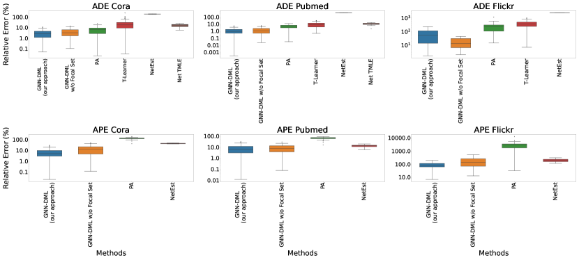
Figure 2: Relative Error of different methods for estimating causal effects across different datasets. Note that the y-axis is log-scaled. In the figure, two variants of our method are presented: one utilizing a focal set and another without a focal set, encompassing the entire dataset. ’PA’ refers to Double Machine Learning combined with predefined aggregates

Table 1 presents the mean squared error (MSE) calculated over 100 simulations for each evaluated method. Furthermore, we illustrate the distribution of relative errors for all methods across the datasets in Figure 2 found in the appendix. Our analysis includes two variations of our framework: one that incorporates a focal set and another that does not, thereby covering the entire dataset.

Across all three semi-synthetic datasets, our GNN-DML approach either matches or exceeds the performance of state-of-the-art methods. This enhancement in performance is credited to (i) the strategic use of GNNs for adeptly addressing network confounders, (ii) a DML framework that not only ensures consistency—even in the face of misspecified nuisance functions—but also secures a faster convergence rate, and (iii) elimination of bias due to regularization used for training GNNs. In comparison, the T-learner tends to exhibit higher relative errors and greater variance in its estimations, which can be traced back to its vulnerability to regularization bias and a generally slower convergence rate. Similarly, DML methods utilizing predefined aggregates (min, max, sum, and average) for network information aggregation fall short, as these aggregates do not capture complex network aggregation functions as effectively as GNNs in realistic data-generative settings. A pivotal aspect of our methodology is the emphasis on focal sets analysis, exploiting the independence between units to enhance performance. This focus has demonstrably outperformed variants of our method that omit focal sets, highlighting the strategic value of considering focal sets in analysis of networked data.

We perform additional empirical estimates investigating the performance of our approach for synthetic data with varying levels of graph density and corresponding effective sample size, as well as investigate the coverage probability of estimated 95% confidence intervals in Appendix 12

6.2 Analysis of Real Data

Data Description: We selected the Indian Village dataset, encompassing a comprehensive survey from Karnataka, India, with data on 16,995 individuals across 77 villages, 15 features, and 12 distinct social networks, for its rich representation of real-world social structures and its potential to shed light on economic and social behaviors within these communities (Banerjee et al.,, 2014; Jackson et al.,, 2012). This dataset provides a unique opportunity to explore the intricate dynamics of social relationships, such as borrowing and lending, advice networks, and more, making it an invaluable resource for understanding the impact of social networks on individual and collective outcomes.

Hypotheses: Utilizing our framework on the Indian Village dataset, we tested hypotheses centered on the influence of self-help group (SHG) participation on financial behaviors. Specifically, we investigated whether individuals’ or their peers’ participation in SHG affects their financial risk-taking behavior. Here, we consider an individual’s participation in the SHG as a binary treatment variable, and having a loan account as the outcome. We hypothesize that SHG participation may enhance individuals’ risk tolerance, observable through the lens of outstanding loans as a proxy measure. This hypothesis aligns with existing research, such as studies by Rajagopal, (2020); Greaney et al., (2016); Attanasio et al., (2023); Gilad et al., (2021), which have underscored the positive effects of SHGs on economic empowerment and risk management. Through our analysis, we aimed to quantify the average direct and indirect effect of these social and group dynamics on individuals’ financial risk-taking behaviors.

Our methodology yielded an average direct effect (ADE) of 0.252, with a 95% confidence interval of $[0.172,0.332]$. This positive ADE indicates that participation in Self-Help Groups (SHGs) has a direct positive impact on individual risk tolerance. Additionally, our analysis identified an average peer effect (APE) of 0.017, with a 95% confidence interval of $[0.007,0.027]$. Although the APE’s magnitude is smaller than that of the ADE, it remains statistically significant and positive, suggesting a beneficial spillover effect that aids individuals in enhancing their risk tolerance. This finding aligns with results reported by Gilad et al. (Gilad et al.,, 2021), who observed a similar direct effect of SHG membership on the probability of possessing an outstanding loan, quantified at 0.30, thereby corroborating the role of SHGs in influencing financial behaviors.

7 Conclusion

Our work proposes a double-machine learning integrated with the graph representation learning techniques to adjust for complex network confounders and efficiently estimate the treatment effect. We evaluate our approach via thorough simulation studies and real data case studies, highlighting its effectiveness.

In future, we aim to adapt our framework for application in relational data scenarios, specifically those involving heterogeneous graphs. Another promising avenue for future exploration involves investigating scenarios where the expressive capacity of message passing Graph Neural Networks (GNNs), limited by the Weisfeiler-Lehman test, may fall short in capturing causal structures. Addressing this limitation could entail exploring higher-order graphs to enhance model expressiveness. Additionally, we intend to investigate the impact of missing network ties on estimation in partially observable graphs and develop strategies to mitigate such challenges. These future directions aim to broaden the scope and applicability of our framework in addressing diverse and complex graph-based causal inference problems.

8 Proof of Identifiability

In this section, we present a detailed, step-by-step proof of the identifiability of the Average Direct Effect (ADE) and the Average Partial Effect (APE), based on the assumptions outlined in Section 3.1.

$$\tau_{ADE} =\mathbb{E}\left[\frac{1}{n}\sum_{i\in\mathcal{V}}\tau_{i,DE}\right]$$ (14)

$$=\mathbb{E}\left[\frac{1}{n}\sum_{i\in\mathcal{V}}Y_{i}(1,\mathbf{T_{-i}})-Y_{i}(0,\mathbf{T_{-i}})\right]=$$ (15)

$$=\mathbb{E}\left[\frac{1}{n}\sum_{i\in\mathcal{V}}Y_{i}(1,\mathbf{T_{\mathbb{N}_{i}}})-Y_{i}(0,\mathbf{T_{\mathbb{N}_{i}}})\right]=$$ (16)

$$=\mathbb{E}\left[\frac{1}{n}\sum_{i\in\mathcal{V}}Y_{i}(1,z_{i})-Y_{i}(0,z_{i})\right]=$$ (17)

$$=\mathbb{E}_{X}\left[\mathbb{E}\left[\frac{1}{n}\sum_{i\in\mathcal{V}}Y_{i}(1,z_{i})-Y_{i}(0,z_{i})\mid\mathcal{X}\right]\right]=$$ (18)

$$=\mathbb{E}_{X}\left[\mathbb{E}\left[\frac{1}{n}\sum_{i\in\mathcal{V}}Y_{i}(1,z_{i})-Y_{i}(0,z_{i})\mid\mathbf{X_{i}},\mathcal{X}_{\mathbb{N}_{i}}\right]\right]=$$ (19)

$$\begin{split}&=\mathbb{E}_{X}\biggl{[}\mathbb{E}\biggl{[}\frac{1}{n}\sum_{i\in\mathcal{V}}Y_{i}(1,z_{i})\mid\mathbf{X_{i}},\mathcal{X}_{\mathbb{N}_{i}},t_{i},z_{i}\biggl{]}-\\ &\quad\mathbb{E}\biggl{[}\frac{1}{n}\sum_{i\in\mathcal{V}}Y_{i}(0,z_{i})\mid\mathbf{X_{i}},\mathcal{X}_{\mathbb{N}_{i}},t_{i},z_{i}\biggl{]}\biggl{]}\end{split}$$ (20)

$$\begin{split}&=\mathbb{E}_{X}\biggl{[}\mathbb{E}\biggl{[}\frac{1}{n}\sum_{i\in\mathcal{V}}Y_{i}\mid\mathbf{X_{i}},\mathcal{X}_{\mathbb{N}_{i}},t_{i}=1,z_{i}\biggl{]}-\\ &\quad\mathbb{E}\biggl{[}\frac{1}{n}\sum_{i\in\mathcal{V}}Y_{i}\mid\mathbf{X_{i}},\mathcal{X}_{\mathbb{N}_{i}},t_{i}=0,z_{i}\biggl{]}\biggl{]}\end{split}$$ (21)

Equation 16 uses partial interference assumption, 17 uses the assumption that the exposure map is well-defined and known, 18 uses law of total expectation, 19 uses partial interference assumption, 20 uses strong ignorability and 21 uses consistency assumption.

$$\tau_{APE} =\mathbb{E}\left[\frac{1}{n}\sum_{i\in\mathcal{V}}\tau_{i,PE}\right]$$ (22)

$$=\mathbb{E}\left[\frac{1}{n}\sum_{i\in\mathcal{V}}Y_{i}(T_{i},\mathbf{1}_{-i})-Y_{i}(T_{i},\mathbf{0}_{-i})\right]=$$ (23)

$$=\mathbb{E}\left[\frac{1}{n}\sum_{i\in\mathcal{V}}Y_{i}(T_{i},\mathbf{T_{\mathbb{N}_{i}}}=\mathbf{1})-Y_{i}(T_{i},\mathbf{T_{\mathbb{N}_{i}}}=\mathbf{0})\right]=$$ (24)

$$=\mathbb{E}\left[\frac{1}{n}\sum_{i\in\mathcal{V}}Y_{i}(T_{i},z_{i}^{\prime})-Y_{i}(T_{i},z_{i}^{\prime\prime})\right]=$$ (25)

$$=\mathbb{E}_{X}\left[\mathbb{E}\left[\frac{1}{n}\sum_{i\in\mathcal{V}}Y_{i}(T_{i},z_{i}^{\prime})-Y_{i}(T_{i},z_{i}^{\prime\prime})\mid\mathcal{X}\right]\right]=$$ (26)

$$=\mathbb{E}_{X}\left[\mathbb{E}\left[\frac{1}{n}\sum_{i\in\mathcal{V}}Y_{i}(T_{i},z_{i}^{\prime})-Y_{i}(T_{i},z_{i}^{\prime\prime})\mid\mathbf{X_{i}},\mathcal{X}_{\mathbb{N}_{i}}\right]\right]=$$ (27)

$$\begin{split}&=\mathbb{E}_{X}\biggl{[}\mathbb{E}\biggl{[}\frac{1}{n}\sum_{i\in\mathcal{V}}Y_{i}(T_{i},z_{i}^{\prime})\mid\mathbf{X_{i}},\mathcal{X}_{\mathbb{N}_{i}},t_{i},z_{i}\biggl{]}-\\ &\quad\mathbb{E}\biggl{[}\frac{1}{n}\sum_{i\in\mathcal{V}}Y_{i}(T_{i},z_{i}^{\prime\prime})\mid\mathbf{X_{i}},\mathcal{X}_{\mathbb{N}_{i}},t_{i},z_{i}\biggl{]}\biggl{]}\end{split}$$ (28)

$$\begin{split}&=\mathbb{E}_{X}\biggl{[}\mathbb{E}\biggl{[}\frac{1}{n}\sum_{i\in\mathcal{V}}Y_{i}\mid\mathbf{X_{i}},\mathcal{X}_{\mathbb{N}_{i}},t_{i},z_{i}=z_{i}^{\prime}\biggl{]}-\\ &\quad\mathbb{E}\biggl{[}\frac{1}{n}\sum_{i\in\mathcal{V}}Y_{i}\mid\mathbf{X_{i}},\mathcal{X}_{\mathbb{N}_{i}},t_{i},z_{i}=z_{i}^{\prime\prime}\biggl{]}\biggl{]}\end{split}$$ (29)

Equation 24 uses partial interference assumption, 25 uses the assumption that the exposure map is well-defined and known, 26 uses law of total expectation, 27 uses partial interference assumption, 28 uses strong ignorability and 29 uses consistency assumption.

9 Derivation of score function

In this section, we introduce the concept of the neyman orthogonal score function and proceed to derive the corresponding score function pertinent to our study. This derivation is structured around our specific set of structural equations and is guided by the methodology outlined in  (Chernozhukov et al.,, 2018).
Let $\zeta\in\mathcal{Z}\subset\mathbb{R}^{d_{\zeta}}$ and $\beta\in\mathcal{B}\subset\mathbb{R}^{d_{\beta}}$ be the target and nuisance parameters respectively. Suppose the true parameter values $\zeta_{0}$ and $\beta_{0}$ that solves the following optimization problem

$$\max_{\zeta\in\mathcal{Z},\beta\in\mathcal{B}}\mathbb{E}_{P}[\mathcal{L}(W;\zeta,\beta)]$$

where $W$ is a random element taking values in a measurable space $(\mathcal{W},\mathcal{A}_{\mathcal{W}})$ with law determined by a probability measure $P\in\mathcal{P}_{n}$ and $\mathcal{L}(W;\zeta,\beta)$ is a known criterion function. $\zeta_{0}$ and $\beta_{0}$ satisfy

$$\mathbb{E}_{P}\left[\partial_{\zeta}\mathcal{L}\left(W;\zeta_{0},\beta_{0}\right)\right]=0,\quad\mathbb{E}_{P}\left[\partial_{\beta}\mathcal{L}\left(W;\zeta_{0},\beta_{0}\right)\right]=0$$

Definition. (neyman orthogonality) The score $\psi=\left(\psi_{1},\ldots,\psi_{d_{\theta}}\right)^{\prime}$ obeys the orthogonality condition at $\left(\theta_{0},\eta_{0}\right)$ with respect to the nuisance realization set $\Gamma_{n}\subset T$ if

$$\mathbb{E}_{P}\left[\psi\left(W;\theta_{0},\eta_{0}\right)\right]=0$$

holds and the pathwise derivative map $\mathrm{D}_{r}\left[\eta-\eta_{0}\right]$ exists for all $r\in[0,1)$ and $\eta\in\Gamma_{n}$ and vanishes at $r=0$; namely,

$$\partial_{\eta}\mathbb{E}_{P}\psi\left(W;\theta_{0},\eta_{0}\right)\left[\eta-\eta_{0}\right]=0,\quad\text{ for all }\eta\in\Gamma_{n}.$$

We remark here that the condition holds with $\Gamma_{n}=T$ when $\eta$ is a finite-dimensional vector as long as $\partial_{\eta}\mathbb{E}_{P}\left[\psi_{j}\left(W;\theta_{0},\eta_{0}\right)\right]=0$ for all $j=1,\ldots,d_{\theta}$, where $\partial_{\eta}\mathbb{E}_{P}\left[\psi_{j}\left(W;\theta_{0},\eta_{0}\right)\right]$ denotes the vector of partial derivatives of the function $\eta\mapsto\mathbb{E}_{P}\left[\psi_{j}\left(W;\theta_{0},\eta\right)\right]$ for $\eta=\eta_{0}$.

The neyman orthogonal score function is

$$\psi(W,\mathcal{A};\zeta,\eta)=\partial_{\zeta}\mathcal{L}(W;\zeta,\beta)-\mu\partial_{\beta}\mathcal{L}(W;\zeta,\beta)$$

where $\psi=(\psi_{1},...,\psi_{d_{\zeta}})^{\prime}$ is a vector of known score functions,the nuisance parameter is

$$\eta=\left(\beta^{\prime},\operatorname{vec}(\mu)^{\prime}\right)^{\prime}\in T=\mathcal{B}\times\mathbb{R}^{d_{\zeta}d_{\beta}}\subset\mathbb{R}^{p},\quad p=d_{\beta}+d_{\zeta}d_{\beta},$$

and $\mu$ is the $d_{\zeta}\times d_{\beta}$ orthogonalization parameter matrix whose true value $\mu_{0}$ solves the equation

$$J_{\zeta\beta}-\mu J_{\beta\beta}=0$$

for

$$J=\left(\begin{array}[]{cc}J_{\zeta\zeta}&J_{\zeta\beta}\\ J_{\beta\zeta}&J_{\beta\beta}\end{array}\right)=\left.\partial_{\left(\zeta^{\prime},\beta^{\prime}\right)}\mathbb{E}_{P}\left[\partial_{\left(\zeta^{\prime},\beta^{\prime}\right)^{\prime}}\mathcal{L}(W;\zeta,\beta)\right]\right|_{\zeta=\zeta_{0};\beta=\beta_{0}}$$

The true value of the nuisance parameter $\eta$ is

$$\eta_{0}=\left(\beta_{0}^{\prime},\operatorname{vec}\left(\mu_{0}\right)^{\prime}\right)^{\prime}$$

and when $J_{\beta\beta}$ is invertible, it has the unique solution,

$$\mu_{0}=J_{\zeta\beta}J_{\beta\beta}^{-1}$$

If $J_{\beta\beta}$ is not invertible, the equation typically has multiple solutions. In this case, it is convenient to focus on a minimal norm solution,

$$\mu_{0}=\arg\min\|\mu\|\text{ such that }\left\|J_{\zeta\beta}-\mu J_{\beta\beta}\right\|_{q}=0$$

for a suitably chosen norm $\|\cdot\|_{q}$ on the space of $d_{\zeta}\times d_{\beta}$ matrices.

In our case, we consider the following criterion function, which is the negative of standard squared loss:

$$\mathbf{\mathcal{L}(W;\zeta,\beta)}_{1\times 1}=-\frac{\mathbf{B}^{\intercal}_{1\times n}\mathbf{B}_{n\times 1}}{2};\quad\mathbf{B}_{n\times 1}=[\mathbf{Y}-\mathbf{\ell(\mathcal{X},\mathcal{A})}-\theta(\mathbf{T}-\mathbf{m(\mathcal{X},\mathcal{A})})-\alpha(\mathcal{A}(\mathbf{T}-\mathbf{m(\mathcal{X},\mathcal{A})}))]$$

where $\zeta=(\theta,\alpha)$ are the target parameters and $\beta=(m,\ell)$ are nuisance parameters. $m$ and $\ell$ are estimates of $m_{0}(\mathcal{X},\mathcal{A})$ and $\ell_{0}(\mathcal{X},\mathcal{A})$ where $m_{0}(\mathcal{X},\mathcal{A})=\mathbb{E}_{P}[T|\mathcal{X},\mathcal{A}]$ and $\ell_{0}(\mathcal{X},\mathcal{A})=\mathbb{E}_{P}[Y|\mathcal{X},\mathcal{A}]$. Thus, we want to solve the following maximization problem and find $\theta_{0}$ and $\alpha_{0}$ such that

$$\theta_{0},\alpha_{0}=\arg\max_{\theta\in\Theta,\alpha\in\triangle}\mathbb{E}_{P}[\mathbf{\mathcal{L}(W;\zeta,\beta)}_{1\times 1}]$$

We take the derivatives to build the score function

$$\partial_{\theta}\mathbf{\mathcal{L}(W;\zeta,\beta)}_{1\times 1} =\mathbf{B}^{\intercal}_{1\times n}(\mathbf{T}-\mathbf{m(\mathcal{X},\mathcal{A})})_{n\times 1}$$

$$\partial_{\alpha}\mathbf{\mathcal{L}(W;\zeta,\beta)}_{1\times 1} =\mathbf{B}^{\intercal}_{1\times n}\mathcal{A}(\mathbf{T}-\mathbf{m(\mathcal{X},\mathcal{A})})_{n\times 1}$$

$$\partial_{m}\mathbf{\mathcal{L}(W;\zeta,\beta)}_{1\times n} =-\mathbf{B}^{\intercal}_{1\times n}(\theta{I_{n}}+\alpha\mathcal{A})_{n\times n}$$

$$\partial_{\ell}\mathbf{\mathcal{L}(W;\zeta,\beta)}_{1\times n} =\mathbf{B}^{\intercal}_{1\times n}{I_{n}}=\mathbf{B}^{\intercal}_{1\times n}$$

$\mathbf{I_{n}}$ is identity matrix with dimension $n\times n$.

Let $\mathbf{B_{0}}_{n\times 1}=\mathbf{Y}-\mathbf{\ell_{0}(\mathcal{X},\mathcal{A})}-\theta_{0}(\mathbf{T}-\mathbf{m_{0}(\mathcal{X},\mathcal{A})})-\alpha_{0}(\mathcal{A}(\mathbf{T}-\mathbf{m_{0}(\mathcal{X},\mathcal{A})}))$

$$J_{\beta\beta}=\left.\partial_{\beta^{\prime}}\mathbb{E}_{P}\left[\partial_{\beta}\mathbf{\mathcal{L}(W;\zeta,\beta)}\right]\right|_{\zeta=\zeta_{0};\beta=\beta_{0}}$$

$$=\left(\begin{array}[]{cc}-[(\theta_{0}{I_{n}}+\alpha_{0}\mathcal{A})^{\intercal}(\theta_{0}{I_{n}}+\alpha_{0}\mathcal{A})]_{n\times n}&[(\theta_{0}{I_{n}}+\alpha_{0}\mathcal{A})^{\intercal}]_{n\times n}\\ \left[(\theta_{0}{I_{n}}+\alpha_{0}\mathcal{A})\right]_{n\times n}&-[{I_{n}}]_{n\times n}\end{array}\right)_{2n\times 2n}\Rightarrow\text{not invertible}$$

Since $J_{\beta\beta}$ is not invertible, we need to find the minimal norm solution

$$\mu_{0}=\arg\min\|\mu\|\text{ such that }\left\|J_{\zeta\beta}-\mu J_{\beta\beta}\right\|_{q}=0$$

Here $\mu_{0}$ and $J_{\zeta\beta}$ are $2\times 2n$ matrices and $J_{\beta\beta}$ is a $2n\times 2n$ matrix.

$$J_{\zeta\beta}=\left.\partial_{\zeta^{\prime}}\mathbb{E}_{P}\left[\partial_{\beta}\mathbf{\mathcal{L}(W;\zeta,\beta)}\right]\right|_{\zeta=\zeta_{0};\beta=\beta_{0}}=$$

$$\left(\begin{array}[]{cc}-\mathbb{E}_{P}[\mathbf{B_{0}}^{\intercal}+(\mathbf{m_{0}(\mathcal{X},\mathcal{A})}-\mathbf{T})^{\intercal}(\theta_{0}I_{n}+\alpha_{0}\mathcal{A})]_{1\times n}&\mathbb{E}_{P}[(\mathbf{m_{0}(\mathcal{X},\mathcal{A})}-\mathbf{T})^{\intercal}]_{1\times n}\\ -\mathbb{E}_{P}[B_{0}^{\intercal}\mathcal{A}+(\mathbf{m_{0}(\mathcal{X},\mathcal{A})}-\mathbf{T})^{\intercal}\mathcal{A}^{\intercal}(\theta_{0}I_{n}+\alpha_{0}\mathcal{A})]_{1\times n}&\mathbb{E}_{P}[(\mathbf{m_{0}(\mathcal{X},\mathcal{A})}-\mathbf{T})^{\intercal}\mathcal{A}^{\intercal}]_{1\times n}\end{array}\right)_{2\times 2n}$$

Since $m_{0}(\mathcal{X},\mathcal{A})=\mathbb{E}_{P}[T|\mathcal{X},\mathcal{A}]$ and $\ell_{0}(\mathcal{X},\mathcal{A})=\mathbb{E}_{P}[Y|\mathcal{X},\mathcal{A}]$, $\mathbb{E}_{P}[m_{0}(\mathcal{X},\mathcal{A})-T]=0$ and $\mathbb{E}_{P}[\ell_{0}(\mathcal{X},\mathcal{A})-Y]=0$. The expectation of multiplication of a fixed matrix in each of these vectors would also be zero because it would be a linear combination of elements with zero expectation. Thus, $J_{\zeta\beta}=0$ and by inspection, due to the fact that $\|.\|\geq 0$, $\mu=\mathbf{0}$ would make this norm minimum.

Hence, the score function would be:

$$\psi(\mathcal{W},\mathcal{A};\zeta,\eta)=\left(\begin{array}[]{cc}(\mathbf{Y}-\mathbf{\ell(\mathcal{X},\mathcal{A})}-\theta(\mathbf{T}-\mathbf{m(\mathcal{X},\mathcal{A})})-\alpha(\mathcal{A}(\mathbf{T}-\mathbf{m(\mathcal{X},\mathcal{A})}))^{\intercal}(\mathbf{T}-\mathbf{m(\mathcal{X},\mathcal{A})})\\ (\mathbf{Y}-\mathbf{\ell(\mathcal{X},\mathcal{A})}-\theta(\mathbf{T}-\mathbf{m(\mathcal{X},\mathcal{A})})-\alpha(\mathcal{A}(\mathbf{T}-\mathbf{m(\mathcal{X},\mathcal{A})}))^{\intercal}\mathcal{A}(\mathbf{T}-\mathbf{m(\mathcal{X},\mathcal{A})})\end{array}\right)$$

10 Proof of Theorem 5.2 and Corresponding Conditions to Verify

In this section, we describe the essential regularity conditions and provide their respective proofs. These conditions form the foundational basis for proving Theorem 5.2. By demonstrating that the score function fulfills specific assumptions, we can effectively invoke Theorems 3.1 and 3.2, along with Corollary 3.1 from  Chernozhukov et al., (2018).
This application is crucial for establishing two key properties of our estimators: consistency and asymptotic normality. These 2 are the asymptotic properties of an estimator. Asymptotic refers to a mathematical property of a sequence of random variables or a statistical estimator as the sample size approaches infinity. More specifically, it refers to the behavior of the estimator as the sample size becomes larger and larger. An asymptotic result holds in the limit as the sample size grows infinitely large.
We say that an estimate $\hat{\theta}$ is consistent if $\hat{\theta}\rightarrow\theta_{0}$ in probability as $n\rightarrow\infty$, where $\theta_{0}$ is the ’true’ unknown parameter of the distribution of the sample.
We say that $\hat{\theta}$ is asymptotically normal if

$$\sqrt{n}\left(\hat{\theta}-\theta_{0}\right)\xrightarrow{\text{d}}\mathcal{N}\left(0,\sigma_{\theta_{0}}^{2}\right)$$

where $\sigma_{\theta_{0}}^{2}$ is called the asymptotic variance of the estimate $\hat{\theta}$. Asymptotic normality says that the estimator not only converges to the unknown parameter, but it converges fast enough, at a rate $1/\sqrt{n}$, where $n$ is the sample size.

These properties are fundamental in reinforcing the statistical robustness and reliability of our estimators in both finite sample and asymptotic contexts. Besides, they allow us to perform uncertainty quantification and build confidence intervals.
The invocation of Theorems 3.1 and 3.2 along with Corollary 3.1 from  Chernozhukov et al., (2018) are sufficient for proving our Theorem 5.2.
In the following discussion, we delve into two distinct sets of conditions as outlined in  Chernozhukov et al., (2018) that are necessary to invoke these theorems.
We use $\|.\|_{P,q}$ to denote the $L^{q}(P)$ norm, i.e. $\|f\|_{P,q}:=\|f(W)\|_{P,q}:=(\int\mid f(w)\mid^{q}dP(w))^{\frac{1}{q}}$.

Assumption 10.1.

(Regularity Conditions) Let $c>0,C>0,c_{1}\geqslant c_{0}>0,q>4$ and $K\geqslant 2$ be some finite constants; and let $\{\delta_{n}\}_{n=1}^{\infty}$ and $\{\Delta_{n}\}_{n=1}^{\infty}$ be some sequences of positive constants converging to zero such that $\delta_{n}\geqslant n_{f}^{-1/2}$. For all probability laws $P\in\mathcal{P}$ for the triple $W=(\mathbf{T},\mathbf{Y},\mathcal{X})$ the following conditions hold:

1. Equation set 3.1 holds

2. $c\leqslant\|\mathbf{\epsilon^{T}}\|_{P,2}$ , $\|\mathbf{\epsilon^{T}}\|_{P,q}\leqslant C$, $\leqslant\|\mathbf{\epsilon^{Y}}\|_{P,q}\leqslant C$

3. $c\leqslant{\|\mathbf{\epsilon^{Y}}^{\intercal}\mathbf{\epsilon^{T}}\|}_{P,2}$, $c\leqslant\mathbb{E}_{P}\left[\mathbf{\epsilon^{T}}^{\intercal}\mathbf{\epsilon^{T}}\right]$, $c\leqslant\mathbb{E}_{P}\left[\mathbf{\epsilon^{T}}^{\intercal}\mathcal{A}^{\intercal}\mathbf{\epsilon^{T}}\right]$

4. $\|\mathbf{Y}\|_{P,q}\leqslant C$

5. $\mathbf{\epsilon^{T}}$ and $\mathbf{\epsilon^{Y}}$ are not eigen vectors of $\mathcal{A}$.

6. Given a random subset $I$ of $[n_{f}]$ of size $n^{\prime}=n_{f}/K$, the nuisance parameter estimator $\widehat{\eta}_{0}=\widehat{\eta}_{0}\left(\left(W_{i}\right)_{i\in I^{c}}\right)$ belongs to the realization set $\mathcal{T}_{n}$ with probability at least $1-\Delta_{n}$, where $\eta_{0}\in\mathcal{T}_{n}$.

7. Given a random subset $I$ of $[n_{f}]$ of size $n^{\prime}=n_{f}/K$, the nuisance parameter estimator $\widehat{\eta}_{0}=\widehat{\eta}_{0}\left(\left(W_{i}\right)_{i\in I^{c}}\right)$ obeys the following conditions: With $P$-probability no less than $1-\Delta_{n}$,

   $$\left\|\widehat{\eta}_{0}-\eta_{0}\right\|_{P,q}\leqslant C,\quad\left\|\widehat{\eta}_{0}-\eta_{0}\right\|_{P,2}\leqslant\delta_{n},\quad\text{ and }$$

   for the score $\psi$, where $\widehat{\eta}_{0}=\left(\widehat{m}_{0},\widehat{\ell}_{0}\right)$,

   $$\left\|\widehat{m}_{0}-m_{0}\right\|_{P,2}\times\left(\left\|\widehat{m}_{0}-m_{0}\right\|_{P,2}+\left\|\widehat{\ell}_{0}-\ell_{0}\right\|_{P,2}\right)\leqslant\delta_{n}n_{f}^{-1/2}.$$

10.1 Condition Set 1: Linear Scores with Approximate Neyman Orthogonality

For all $n_{f}\geqslant 3$ and probability measures $P\in\mathcal{P}_{n}$ that determines the underlying law of $W$:

1. Moment condition vanishes at the true parameter $\zeta_{0}$: $\mathbb{E}_{P}\left[\psi\left(W;\zeta_{0},\eta_{0}\right)\right]=0$

2. The score function is linear in the sense that: $\psi(W,\mathcal{A};\zeta,\eta)=\psi^{a}(W,\mathcal{A};\zeta,\eta)\theta+\psi^{b}(W;\zeta,\eta)\alpha+\psi^{c}(W;\zeta,\eta)$

3. The map $\eta\rightarrow\mathbb{E}_{P}\left[\psi\left(W;\zeta_{0},\eta_{0}\right)\right]$ is twice continuously Gateaux-differentiable.

4. The score $\psi$ is Neyman orthogonal or, more generally, it is Neyman $\lambda_{n}$ near-orthogonal at $\left(\zeta_{0},\eta_{0}\right)$ with respect to the nuisance realization set $\Gamma_{n}\subset T$ for

   $$\lambda_{n}:=\sup_{\eta\in\Gamma_{n}}\left\|\partial_{\eta}\mathbb{E}_{P}\psi\left(W;\zeta_{0},\eta_{0}\right)\left[\eta-\eta_{0}\right]\right\|\leqslant\delta_{n}n_{f}^{-1/2}$$

5. The identification condition holds; namely, the singular values of the matrix

   $$J_{0,a}:=\mathbb{E}_{P}\left[\psi^{a}\left(W;\eta_{0}\right)\right]$$

   are between $c_{0}$ and $c_{1}$.

10.2 Condition Set 2: Score Regularity and Quality of nuisance Parameter Estimators

For all $n_{f}\geqslant 3$ and $P\in\mathcal{P}_{n}$, the following conditions hold:

1. Given a random subset $I$ of $[n_{f}]$ of size $n^{\prime}=n_{f}/K$, the nuisance parameter estimator $\widehat{\eta}_{0}=\widehat{\eta}_{0}\left(\left(W_{i}\right)_{i\in I^{c}}\right)$ belongs to the realization set $\Gamma_{n}$ with probability at least $1-\Delta_{n}$, where $\Gamma_{n}$ contains $\eta_{0}$ and is constrained by the next conditions.

2. The moment conditions hold:

   $$m_{n}:=\sup_{\eta\in\Gamma_{n}}\left(\mathbb{E}_{P}\left[\left\|\psi\left(W;\zeta_{0},\eta\right)\right\|^{q}\right]\right)^{1/q}\leqslant c_{1},$$

   $$m_{n}^{\prime}:=\sup_{\eta\in\Gamma_{n}}\left(\mathbb{E}_{P}\left[\left\|\psi^{a}(W;\eta)\right\|^{q}\right]\right)^{1/q}\leqslant c_{1}.$$

3. The following conditions on the statistical rates $r_{n},r_{n}^{\prime}$, and $\lambda_{n}^{\prime}$ hold:

   $$r_{n}:=\sup_{\eta\in\Gamma_{n}}\left\|\mathbb{E}_{P}\left[\psi^{a}(W;\eta)\right]-\mathbb{E}_{P}\left[\psi^{a}\left(W;\eta_{0}\right)\right]\right\|\leqslant\delta_{n},$$

   $$r_{n}^{\prime}:=\sup_{\eta\in\Gamma_{n}}\left(\mathbb{E}_{P}\left[\left\|\psi\left(W;\zeta_{0},\eta\right)-\psi\left(W;\zeta_{0},\eta_{0}\right)\right\|^{2}\right]\right)^{1/2}\leqslant\delta_{n},$$

   $$\lambda_{n}^{\prime}:=\sup_{r\in(0,1),\eta\in\Gamma_{n}}\left\|\partial_{r}^{2}\mathbb{E}_{P}\left[\psi\left(W;\zeta_{0},\eta_{0}+r\left(\eta-\eta_{0}\right)\right)\right]\right\|\leqslant\delta_{n}/\sqrt{n_{f}}.$$

4. The variance of the score $\psi$ is non-degenerate: All eigenvalues of the matrix

   $$\mathbb{E}_{P}\left[\psi\left(W;\zeta_{0},\eta_{0}\right)\psi\left(W;\zeta_{0},\eta_{0}\right)^{\prime}\right]$$

   are bounded from below by $c_{0}$.

In the rest of this section, we attempt to prove the condition sets 10.1 and 10.2 under regularity assumptions 10.1.

10.3 Proof of Condition Set 1

C.1.1

The true parameter values $\zeta_{0}$ and $\beta_{0}$ solve the following optimization problem

$$\max_{\zeta\in\mathcal{Z},\beta\in\mathcal{B}}\mathbb{E}_{P}[\mathcal{L}(W;\zeta,\beta)]$$

where $\mathcal{L}(W;\zeta,\beta)$ is a known criterion function. $\zeta_{0}$ and $\beta_{0}$ satisfy

$$\mathbb{E}_{P}\left[\partial_{\zeta}\mathcal{L}\left(W;\zeta_{0},\beta_{0}\right)\right]=0,\quad\mathbb{E}_{P}\left[\partial_{\beta}\mathcal{L}\left(W;\zeta_{0},\beta_{0}\right)\right]=0$$

The neyman orthogonal score function is

$$\psi(W,\mathcal{A};\zeta,\eta)=\partial_{\zeta}\mathcal{L}(W;\zeta,\beta)-\mu\partial_{\beta}\mathcal{L}(W;\zeta,\beta)$$

Thus, by definition of $\zeta_{0}$ and $\eta_{0}$, we have:

$$\mathbb{E}_{P}\left[\psi\left(W;\zeta_{0},\eta_{0}\right)\right]=0$$

C.1.2

The score function is linear in the sense that:

$$\psi(W,\mathcal{A};\zeta,\eta)=\left(\begin{array}[]{cc}(\mathbf{Y}-\mathbf{\ell(\mathcal{X},\mathcal{A})}-\theta(\mathbf{T}-\mathbf{m(\mathcal{X},\mathcal{A})})-\alpha(\mathcal{A}(\mathbf{T}-\mathbf{m(\mathcal{X},\mathcal{A})}))^{\intercal}(\mathbf{T}-\mathbf{m(\mathcal{X},\mathcal{A})})\\ (\mathbf{Y}-\mathbf{\ell(\mathcal{X},\mathcal{A})}-\theta(\mathbf{T}-\mathbf{m(\mathcal{X},\mathcal{A})})-\alpha(\mathcal{A}(\mathbf{T}-\mathbf{m(\mathcal{X},\mathcal{A})}))^{\intercal}\mathcal{A}(\mathbf{T}-\mathbf{m(\mathcal{X},\mathcal{A})})\end{array}\right)=$$ (34)

$$\underbrace{\left(\begin{array}[]{cccc}-(\mathbf{T}-\mathbf{m(\mathcal{X},\mathcal{A})})^{\intercal}(\mathbf{T}-\mathbf{m(\mathcal{X},\mathcal{A})})&-(\mathbf{T}-\mathbf{m(\mathcal{X},\mathcal{A})})^{\intercal}\mathcal{A}^{\intercal}(\mathbf{T}-\mathbf{m(\mathcal{X},\mathcal{A})})\\ -(\mathbf{T}-\mathbf{m(\mathcal{X},\mathcal{A})})^{\intercal}\mathcal{A}(\mathbf{T}-\mathbf{m(\mathcal{X},\mathcal{A})})&-(\mathbf{T}-\mathbf{m(\mathcal{X},\mathcal{A})})^{\intercal}\mathcal{A}^{\intercal}\mathcal{A}(\mathbf{T}-\mathbf{m(\mathcal{X},\mathcal{A})})\end{array}\right)}_{\psi^{a}}\left(\begin{array}[]{cc}\theta\\ \alpha\end{array}\right)+\underbrace{\left(\begin{array}[]{cc}(\mathbf{Y}-\mathbf{\ell(\mathcal{X},\mathcal{A})})^{\intercal}(\mathbf{T}-\mathbf{m(\mathcal{X},\mathcal{A})})\\ (\mathbf{Y}-\mathbf{\ell(\mathcal{X},\mathcal{A})})^{\intercal}\mathcal{A}(\mathbf{T}-\mathbf{m(\mathcal{X},\mathcal{A})})\end{array}\right)}_{\psi^{b}}$$ (41)

C.1.3

The score function can trivially be shown to be twice Gateaux differentiable.

C.1.4

To show neyman orthogonality, we need to show that Gateaux derivative vanishes in addition to the moment condition. The Gateaux derivative in the direction $\eta-\eta_{0}=(\mathbf{m}-\mathbf{m_{0}},\mathbf{\ell}-\mathbf{\ell_{0}})$ is:

$$\partial_{\eta}\mathbb{E}_{P}\psi\left(W;\zeta_{0},\eta_{0}\right)\left[\eta-\eta_{0}\right]=\\ \\ {\lim\limits_{r\to 0}\frac{\begin{multlined}\mathbb{E}_{P}\left(\begin{array}[]{cc}(\mathbf{Y}-(\mathbf{\ell_{0}}+r(\mathbf{\ell}-\mathbf{\ell_{0}}))-\theta_{0}(\mathbf{T}-(\mathbf{m_{0}}+r(\mathbf{m}-\mathbf{m_{0}})))-\alpha_{0}(\mathcal{A}(\mathbf{T}-(\mathbf{m_{0}}+r(\mathbf{m}-\mathbf{m_{0}})))))^{\intercal}(\mathbf{T}-(\mathbf{m_{0}}+r(\mathbf{m}-\mathbf{m_{0}})))\\ (\mathbf{Y}-(\mathbf{\ell_{0}}+r(\mathbf{\ell}-\mathbf{\ell_{0}}))-\theta_{0}(\mathbf{T}-(\mathbf{m_{0}}+r(\mathbf{m}-\mathbf{m_{0}})))-\alpha_{0}(\mathcal{A}(\mathbf{T}-(\mathbf{m_{0}}+r(\mathbf{m}-\mathbf{m_{0}})))))^{\intercal}\mathcal{A}(\mathbf{T}-(\mathbf{m_{0}}+r(\mathbf{m}-\mathbf{m_{0}})))\end{array}\right)\\ -\mathbb{E}_{P}\left(\begin{array}[]{cc}(\mathbf{Y}-\mathbf{\ell_{0}}-\theta_{0}(\mathbf{T}-\mathbf{m_{0}})-\alpha_{0}(\mathcal{A}(\mathbf{T}-\mathbf{m_{0}}))^{\intercal}(\mathbf{T}-\mathbf{m_{0}})\\ (\mathbf{Y}-\mathbf{\ell_{0}}-\theta_{0}(\mathbf{T}-\mathbf{m_{0}})-\alpha_{0}(\mathcal{A}(\mathbf{T}-\mathbf{m_{0}}))^{\intercal}\mathcal{A}(\mathbf{T}-\mathbf{m_{0}})\end{array}\right)\end{multlined}\mathbb{E}_{P}\left(\begin{array}[]{cc}(\mathbf{Y}-(\mathbf{\ell_{0}}+r(\mathbf{\ell}-\mathbf{\ell_{0}}))-\theta_{0}(\mathbf{T}-(\mathbf{m_{0}}+r(\mathbf{m}-\mathbf{m_{0}})))-\alpha_{0}(\mathcal{A}(\mathbf{T}-(\mathbf{m_{0}}+r(\mathbf{m}-\mathbf{m_{0}})))))^{\intercal}(\mathbf{T}-(\mathbf{m_{0}}+r(\mathbf{m}-\mathbf{m_{0}})))\\ (\mathbf{Y}-(\mathbf{\ell_{0}}+r(\mathbf{\ell}-\mathbf{\ell_{0}}))-\theta_{0}(\mathbf{T}-(\mathbf{m_{0}}+r(\mathbf{m}-\mathbf{m_{0}})))-\alpha_{0}(\mathcal{A}(\mathbf{T}-(\mathbf{m_{0}}+r(\mathbf{m}-\mathbf{m_{0}})))))^{\intercal}\mathcal{A}(\mathbf{T}-(\mathbf{m_{0}}+r(\mathbf{m}-\mathbf{m_{0}})))\end{array}\right)\\ -\mathbb{E}_{P}\left(\begin{array}[]{cc}(\mathbf{Y}-\mathbf{\ell_{0}}-\theta_{0}(\mathbf{T}-\mathbf{m_{0}})-\alpha_{0}(\mathcal{A}(\mathbf{T}-\mathbf{m_{0}}))^{\intercal}(\mathbf{T}-\mathbf{m_{0}})\\ (\mathbf{Y}-\mathbf{\ell_{0}}-\theta_{0}(\mathbf{T}-\mathbf{m_{0}})-\alpha_{0}(\mathcal{A}(\mathbf{T}-\mathbf{m_{0}}))^{\intercal}\mathcal{A}(\mathbf{T}-\mathbf{m_{0}})\end{array}\right)}{r}}=\\ \\ {\lim\limits_{r\to 0}\frac{\begin{multlined}\mathbb{E}_{P}\left(\begin{array}[]{cc}(\overbrace{\mathbf{Y}-\mathbf{\ell_{0}}-\theta_{0}(\mathbf{T}-\mathbf{m_{0}})-\alpha_{0}(\mathcal{A}(\mathbf{T}-\mathbf{m_{0}}-r(\mathbf{m}-\mathbf{m_{0}})))}^{\mathbf{\epsilon^{Y}}}-\overbrace{r(\mathbf{\ell}-\mathbf{\ell_{0}})}^{\mathbf{G}}+\overbrace{\theta_{0}r(\mathbf{m}-\mathbf{m_{0}})}^{\theta_{0}\mathbf{D}}+\overbrace{\alpha_{0}\mathcal{A}r(\mathbf{m}-\mathbf{m_{0}})}^{\alpha_{0}\mathcal{A}\mathbf{D}})^{\intercal}(\overbrace{\mathbf{T}-\mathbf{m_{0}}}^{\mathbf{\epsilon^{T}}}-\overbrace{r(\mathbf{m}-\mathbf{m_{0}})}^{\mathbf{D}})\\ (\mathbf{Y}-\mathbf{\ell_{0}}-\theta_{0}(\mathbf{T}-\mathbf{m_{0}})-\alpha_{0}(\mathcal{A}(\mathbf{T}-\mathbf{m_{0}}-r(\mathbf{m}-\mathbf{m_{0}})))-r(\mathbf{\ell}-\mathbf{\ell_{0}})+\theta_{0}r(\mathbf{m}-\mathbf{m_{0}})+\alpha_{0}\mathcal{A}r(\mathbf{m}-\mathbf{m_{0}}))^{\intercal}\mathcal{A}(\mathbf{T}-\mathbf{m_{0}}-r(\mathbf{m}-\mathbf{m_{0}}))\end{array}\right)\\ -\mathbb{E}_{P}\left(\begin{array}[]{cc}(\overbrace{{\mathbf{Y}-\mathbf{\ell_{0}}-\theta_{0}(\mathbf{T}-\mathbf{m_{0}})-\alpha_{0}(\mathcal{A}(\mathbf{T}-\mathbf{m_{0}}))}^{\intercal}}^{\mathbf{\epsilon^{Y}}^{\intercal}}\overbrace{(\mathbf{T}-\mathbf{m_{0}})}^{\mathbf{\epsilon}^{T}}\\ (\mathbf{Y}-\mathbf{\ell_{0}}-\theta_{0}(\mathbf{T}-\mathbf{m_{0}})-\alpha_{0}(\mathcal{A}(\mathbf{T}-\mathbf{m_{0}}))^{\intercal}\mathcal{A}(\mathbf{T}-\mathbf{m_{0}})\end{array}\right)\end{multlined}\mathbb{E}_{P}\left(\begin{array}[]{cc}(\overbrace{\mathbf{Y}-\mathbf{\ell_{0}}-\theta_{0}(\mathbf{T}-\mathbf{m_{0}})-\alpha_{0}(\mathcal{A}(\mathbf{T}-\mathbf{m_{0}}-r(\mathbf{m}-\mathbf{m_{0}})))}^{\mathbf{\epsilon^{Y}}}-\overbrace{r(\mathbf{\ell}-\mathbf{\ell_{0}})}^{\mathbf{G}}+\overbrace{\theta_{0}r(\mathbf{m}-\mathbf{m_{0}})}^{\theta_{0}\mathbf{D}}+\overbrace{\alpha_{0}\mathcal{A}r(\mathbf{m}-\mathbf{m_{0}})}^{\alpha_{0}\mathcal{A}\mathbf{D}})^{\intercal}(\overbrace{\mathbf{T}-\mathbf{m_{0}}}^{\mathbf{\epsilon^{T}}}-\overbrace{r(\mathbf{m}-\mathbf{m_{0}})}^{\mathbf{D}})\\ (\mathbf{Y}-\mathbf{\ell_{0}}-\theta_{0}(\mathbf{T}-\mathbf{m_{0}})-\alpha_{0}(\mathcal{A}(\mathbf{T}-\mathbf{m_{0}}-r(\mathbf{m}-\mathbf{m_{0}})))-r(\mathbf{\ell}-\mathbf{\ell_{0}})+\theta_{0}r(\mathbf{m}-\mathbf{m_{0}})+\alpha_{0}\mathcal{A}r(\mathbf{m}-\mathbf{m_{0}}))^{\intercal}\mathcal{A}(\mathbf{T}-\mathbf{m_{0}}-r(\mathbf{m}-\mathbf{m_{0}}))\end{array}\right)\\ -\mathbb{E}_{P}\left(\begin{array}[]{cc}(\overbrace{{\mathbf{Y}-\mathbf{\ell_{0}}-\theta_{0}(\mathbf{T}-\mathbf{m_{0}})-\alpha_{0}(\mathcal{A}(\mathbf{T}-\mathbf{m_{0}}))}^{\intercal}}^{\mathbf{\epsilon^{Y}}^{\intercal}}\overbrace{(\mathbf{T}-\mathbf{m_{0}})}^{\mathbf{\epsilon}^{T}}\\ (\mathbf{Y}-\mathbf{\ell_{0}}-\theta_{0}(\mathbf{T}-\mathbf{m_{0}})-\alpha_{0}(\mathcal{A}(\mathbf{T}-\mathbf{m_{0}}))^{\intercal}\mathcal{A}(\mathbf{T}-\mathbf{m_{0}})\end{array}\right)}{r}}\\ \\ ={\lim\limits_{r\to 0}\frac{\mathbb{E}_{P}\left(\begin{array}[]{cc}\cancel{{\mathbf{\epsilon^{Y}}}^{\intercal}\mathbf{\epsilon^{T}}}-{\mathbf{\epsilon^{Y}}}^{\intercal}\mathbf{D}-\mathbf{G}^{\intercal}\mathbf{\epsilon^{T}}+\theta_{0}\mathbf{D}^{\intercal}\mathbf{\epsilon^{T}}\overbrace{+\mathbf{G}\mathbf{D}-\theta_{0}\mathbf{D}^{\intercal}\mathbf{D}-\alpha_{0}\mathbf{D}^{\intercal}\mathcal{A}^{\intercal}\mathbf{D}}^{\text{goes to 0 includes }r^{2}}+\alpha_{0}\mathbf{D}^{\intercal}\mathcal{A}^{\intercal}\mathbf{\epsilon^{T}}-\cancel{{\mathbf{\epsilon^{Y}}}^{\intercal}\mathbf{\epsilon^{T}}}\\ \cancel{{\mathbf{\epsilon^{Y}}}^{\intercal}\mathcal{A}\mathbf{\epsilon^{T}}}-{\mathbf{\epsilon^{Y}}}^{\intercal}\mathcal{A}\mathbf{D}-\mathbf{G}^{\intercal}\mathcal{A}\mathbf{\epsilon^{T}}+\theta_{0}\mathbf{D}^{\intercal}\mathcal{A}\mathbf{\epsilon^{T}}\overbrace{+\mathbf{G}\mathcal{A}\mathbf{D}-\theta_{0}\mathbf{D}^{\intercal}\mathcal{A}\mathbf{D}-\alpha_{0}\mathbf{D}^{\intercal}\mathcal{A}^{\intercal}\mathcal{A}\mathbf{D}}^{\text{goes to 0 includes }r^{2}}+\alpha_{0}\mathbf{D}^{\intercal}\mathcal{A}^{\intercal}\mathcal{A}\mathbf{\epsilon^{T}}-\cancel{{\mathbf{\epsilon^{Y}}}^{\intercal}\mathcal{A}\mathbf{\epsilon^{T}}}\end{array}\right)}{r}}\\ \\ ={\lim\limits_{r\to 0}\frac{\cancel{r}\mathbb{E}_{P}\left(\begin{array}[]{cc}-{\epsilon^{Y}}^{\intercal}(\mathbf{m}-\mathbf{m_{0}})-(\mathbf{\ell}-\mathbf{\ell_{0}})^{\intercal}\mathbf{\epsilon^{T}}+\theta_{0}(\mathbf{m}-\mathbf{m_{0}})^{\intercal}\mathbf{\epsilon^{T}}+\alpha_{0}(\mathbf{m}-\mathbf{m_{0}})^{\intercal}\mathcal{A}^{\intercal}\mathbf{\epsilon^{T}}\\ -{\epsilon^{Y}}^{\intercal}\mathcal{A}(\mathbf{m}-\mathbf{m_{0}})-(\mathbf{\ell}-\mathbf{\ell_{0}})^{\intercal}\mathcal{A}\mathbf{\epsilon^{T}}+\theta_{0}(\mathbf{m}-\mathbf{m_{0}})^{\intercal}\mathcal{A}\mathbf{\epsilon^{T}}+\alpha_{0}(\mathbf{m}-\mathbf{m_{0}})^{\intercal}\mathcal{A}^{\intercal}\mathcal{A}\mathbf{\epsilon^{T}}\end{array}\right)}{\cancel{r}}}\\ \\ ={\mathbb{E}_{P}\left(\begin{array}[]{cc}-{\epsilon^{Y}}^{\intercal}(\mathbf{m}-\mathbf{m_{0}})-(\mathbf{\ell}-\mathbf{\ell_{0}})^{\intercal}\mathbf{\epsilon^{T}}+\theta_{0}(\mathbf{m}-\mathbf{m_{0}})^{\intercal}\mathbf{\epsilon^{T}}+\alpha_{0}(\mathbf{m}-\mathbf{m_{0}})^{\intercal}\mathcal{A}^{\intercal}\mathbf{\epsilon^{T}}\\ -{\epsilon^{Y}}^{\intercal}\mathcal{A}(\mathbf{m}-\mathbf{m_{0}})-(\mathbf{\ell}-\mathbf{\ell_{0}})^{\intercal}\mathcal{A}\mathbf{\epsilon^{T}}+\theta_{0}(\mathbf{m}-\mathbf{m_{0}})^{\intercal}\mathcal{A}\mathbf{\epsilon^{T}}+\alpha_{0}(\mathbf{m}-\mathbf{m_{0}})^{\intercal}\mathcal{A}^{\intercal}\mathcal{A}\mathbf{\epsilon^{T}}\end{array}\right)}$$

Consider the first term in the above expectation. We use Law of Iterated Expectations:

$$\mathbb{E}_{P}[{\epsilon^{Y}}^{\intercal}(\mathbf{m}-\mathbf{m_{0}})]=\mathbb{E}_{X,D,Y}[{\epsilon^{Y}}^{\intercal}(\mathbf{m}-\mathbf{m_{0}})]=\mathbb{E}_{X}[\mathbb{E}_{YT\mid X}[{\epsilon^{Y}}^{\intercal}\overbrace{(\mathbf{m}-\mathbf{m_{0}})}^{\text{constant given X}}\mid X]]=\mathbb{E}_{X}[(\mathbf{m}-\mathbf{m_{0}})\mathbb{E}_{YT\mid X}[\overbrace{({\epsilon^{Y}}^{\intercal})\mid X}^{0}]]=0$$

A similar argument can be used to show that other expectation terms are $0$.

C.1.5

$$J_{0,a}:=\mathbb{E}_{P}\left[\psi^{a}\left(W;\eta_{0}\right)\right]$$

$$=\mathbb{E}_{P}\left[\left(\begin{array}[]{cccc}-(\mathbf{T}-\mathbf{m_{0}(\mathcal{X},\mathcal{A})})^{\intercal}(\mathbf{T}-\mathbf{m_{0}(\mathcal{X},\mathcal{A})})&-(\mathbf{T}-\mathbf{m_{0}(\mathcal{X},\mathcal{A})})^{\intercal}\mathcal{A}^{\intercal}(\mathbf{T}-\mathbf{m_{0}(\mathcal{X},\mathcal{A})})\\ -(\mathbf{T}-\mathbf{m_{0}(\mathcal{X},\mathcal{A})})^{\intercal}\mathcal{A}(\mathbf{T}-\mathbf{m_{0}(\mathcal{X},\mathcal{A})})&-(\mathbf{T}-\mathbf{m_{0}(\mathcal{X},\mathcal{A})})^{\intercal}\mathcal{A}^{\intercal}\mathcal{A}(\mathbf{T}-\mathbf{m_{0}(\mathcal{X},\mathcal{A})})\end{array}\right)\right]$$

$$=\left(\begin{array}[]{cccc}\mathbf{A_{1}}&\mathbf{A_{2}}\\ \mathbf{A_{3}}&\mathbf{A_{4}}\end{array}\right)$$

$$J_{0,a}^{\intercal}J_{0,a} =\left(\begin{array}[]{cccc}\mathbf{A_{1}}&\mathbf{A_{3}}\\ \mathbf{A_{2}}&\mathbf{A_{4}}\end{array}\right)\left(\begin{array}[]{cccc}\mathbf{A_{1}}&\mathbf{A_{2}}\\ \mathbf{A_{3}}&\mathbf{A_{4}}\end{array}\right)=\left(\begin{array}[]{cccc}\mathbf{A_{1}}^{2}+\mathbf{A_{3}}^{2}&\mathbf{A_{1}}\mathbf{A_{2}}+\mathbf{A_{3}}\mathbf{A_{4}}\\ \mathbf{A_{1}}\mathbf{A_{2}}+\mathbf{A_{3}}\mathbf{A_{4}}&\mathbf{A_{2}}^{2}+\mathbf{A_{4}}^{2}\end{array}\right)$$ (50)

The eigen values of this matrix are the roots of the following quadratic equation:

$$\lambda^{2}-\lambda(\mathbf{A_{1}}^{2}+\mathbf{A_{2}}^{2}+\mathbf{A_{3}}^{2}+\mathbf{A_{4}}^{2})+(\mathbf{A_{1}}^{2}+\mathbf{A_{3}}^{2})(\mathbf{A_{2}}^{2}+\mathbf{A_{4}}^{2})-(\mathbf{A_{1}}\mathbf{A_{2}}+\mathbf{A_{3}}\mathbf{A_{4}})^{2}=0$$

We know that in a quadratic equation of form $a_{2}x^{2}+a_{1}x+a_{0}=0$, the sum of the roots are $\frac{-a_{1}}{a_{2}}$ and the product of the roots are $\frac{a_{0}}{a_{2}}$. To ensure that all the eigen values are positive, we need to make sure both $\frac{-a_{1}}{a_{2}}$ and $\frac{a_{0}}{a_{2}}$ are positive:

$$\frac{-a_{1}}{a_{2}}=\mathbf{A_{1}}^{2}+\mathbf{A_{2}}^{2}+\mathbf{A_{3}}^{2}+\mathbf{A_{4}}^{2}\geqslant c>0$$ (51)

$$\frac{a_{0}}{a_{2}}=(\mathbf{A_{1}}^{2}+\mathbf{A_{3}}^{2})(\mathbf{A_{2}}^{2}+\mathbf{A_{4}}^{2})-(\mathbf{A_{1}}\mathbf{A_{2}}+\mathbf{A_{3}}\mathbf{A_{4}})^{2}=(A_{1}A_{4}-A_{2}A_{3})^{2}$$ (52)

51 holds since the summation of squared elements are non-negative and $A_{1}^{2}=\mathbb{E}_{P}[(\mathbf{T}-\mathbf{m_{0}(\mathcal{X},\mathcal{A})})^{\intercal}(\mathbf{T}-\mathbf{m_{0}(\mathcal{X},\mathcal{A})})]^{2}=\|\mathbf{\epsilon^{T}}\|\geqslant c$ by assumption 2. For 52 to hold, since the squared value is non-negative, we need to show it is not zero, i.e. $A_{1}A_{4}\neq A_{2}A_{3}$. By Cauchy-Schwarz inequality, we know that:

$$\mathbb{E}_{P}\left[\mathbf{\epsilon^{T}}^{\intercal}\mathbf{\epsilon^{T}}\right]\mathbb{E}_{P}\left[\mathbf{\epsilon^{T}}^{\intercal}\mathcal{A}^{\intercal}\mathcal{A}\mathbf{\epsilon^{T}}\right]\geqslant\mathbb{E}_{P}\left[\mathbf{\epsilon^{T}}^{\intercal}\mathcal{A}\mathbf{\epsilon^{T}}\right]^{2}$$

where the equality holds if $\|\mathbf{\epsilon^{T}}\|=0$ or $\|\mathcal{A}\mathbf{\epsilon^{T}}\|=0$, which does not hold by assumption 2 and the fact that $\mathcal{A}$ is a non-zero matrix. Also the equality can happen if $\exists r:\mathcal{A}\mathbf{\epsilon^{T}}=r\mathbf{\epsilon^{T}}$, which does not hold by assumption 5. Thus, summation and product of the eigen values are positive, leading to positivity of the singular values of $J_{0,a}$.

Following proposition is derived from  (Gallier and Quaintance,, 2023):

Proposition 10.2.

For every norm $\|\|$ on $\mathbb{C}^{n}\left(\right.$ or $\left.\mathbb{R}^{n}\right)$, for every matrix $A\in\mathrm{M}_{n}(\mathbb{C})$ (or $A\in\mathrm{M}_{n}(\mathbb{R})$ ), there is a real constant $C_{A}\geqslant 0$, such that

$$\|Au\|\leq C_{A}\|u\|,$$

for every vector $u\in\mathbb{C}^{n}$ (or $u\in\mathbb{R}^{n}$ if $A$ is real).

10.2 states that every linear map on a finite-dimensional space is bounded.

10.4 Proof of Condition Set 2

C.2.1

Condition C.2.1 holds by the construction of the set $\Gamma_{n}$ and Assumption 6.

C.2.2

We prove the boundedness of norms of these matrices by showing the bound on the norm of the elements considering the fact that if norm of each element is bounded, then the norm of the matrix is bounded. We first show the bound for the first elements of $\psi_{a}$ and $\psi$.:

$$\psi^{a}(W;\eta)=\left(\begin{array}[]{cccc}-(\mathbf{T}-\mathbf{m(\mathcal{X},\mathcal{A})})^{\intercal}(\mathbf{T}-\mathbf{m(\mathcal{X},\mathcal{A})})&-(\mathbf{T}-\mathbf{m(\mathcal{X},\mathcal{A})})^{\intercal}\mathcal{A}^{\intercal}(\mathbf{T}-\mathbf{m(\mathcal{X},\mathcal{A})})\\ -(\mathbf{T}-\mathbf{m(\mathcal{X},\mathcal{A})})^{\intercal}\mathcal{A}(\mathbf{T}-\mathbf{m(\mathcal{X},\mathcal{A})})&-(\mathbf{T}-\mathbf{m(\mathcal{X},\mathcal{A})})^{\intercal}\mathcal{A}^{\intercal}\mathcal{A}(\mathbf{T}-\mathbf{m(\mathcal{X},\mathcal{A})})\end{array}\right)$$

$$\psi(W;\zeta_{0},\eta)=\left(\begin{array}[]{cc}(\mathbf{Y}-\mathbf{\ell(\mathcal{X},\mathcal{A})}-\theta_{0}(\mathbf{T}-\mathbf{m(\mathcal{X},\mathcal{A})})-\alpha_{0}(\mathcal{A}(\mathbf{T}-\mathbf{m(\mathcal{X},\mathcal{A})}))^{\intercal}(\mathbf{T}-\mathbf{m(\mathcal{X},\mathcal{A})})\\ (\mathbf{Y}-\mathbf{\ell(\mathcal{X},\mathcal{A})}-\theta_{0}(\mathbf{T}-\mathbf{m(\mathcal{X},\mathcal{A})})-\alpha_{0}(\mathcal{A}(\mathbf{T}-\mathbf{m(\mathcal{X},\mathcal{A})}))^{\intercal}\mathcal{A}(\mathbf{T}-\mathbf{m(\mathcal{X},\mathcal{A})})\end{array}\right)$$

$$\left(\mathbb{E}_{P}\left[\left\|\psi_{11}^{a}(W;\eta)\right\|^{q/2}\right]\right)^{2/q}=\left\|\psi_{11}^{a}(W;\eta)\right\|_{P,q/2}=\left\|-(\mathbf{T}-\mathbf{m(\mathcal{X},\mathcal{A})})^{\intercal}(\mathbf{T}-\mathbf{m(\mathcal{X},\mathcal{A})}\right\|_{P,q/2}=$$

$$\left\|-((\mathbf{T}-\mathbf{m_{0}(\mathcal{X},\mathcal{A})})-(\mathbf{m(\mathcal{X},\mathcal{A})}-\mathbf{m_{0}(\mathcal{X},\mathcal{A})}))^{\intercal}((\mathbf{T}-\mathbf{m_{0}(\mathcal{X},\mathcal{A})})-(\mathbf{m(\mathcal{X},\mathcal{A})}-\mathbf{m_{0}(\mathcal{X},\mathcal{A})}))\right\|_{P,q/2}=$$

$$\left\|((\mathbf{m(\mathcal{X},\mathcal{A})}-\mathbf{m_{0}(\mathcal{X},\mathcal{A})})-\mathbf{\epsilon^{T}})^{\intercal}(\mathbf{\epsilon^{T}}-(\mathbf{m(\mathcal{X},\mathcal{A})}-\mathbf{m_{0}(\mathcal{X},\mathcal{A})}))\right\|_{P,q/2}=$$

$$\bigl{\|}(\mathbf{m(\mathcal{X},\mathcal{A})}-\mathbf{m_{0}(\mathcal{X},\mathcal{A})})^{\intercal}\mathbf{\epsilon^{T}}-(\mathbf{m(\mathcal{X},\mathcal{A})}-\mathbf{m_{0}(\mathcal{X},\mathcal{A})})^{\intercal}(\mathbf{m(\mathcal{X},\mathcal{A})}-\mathbf{m_{0}(\mathcal{X},\mathcal{A})})-\mathbf{\epsilon^{T}}^{\intercal}\mathbf{\epsilon^{T}}+$$

$$\mathbf{\epsilon^{T}}^{\intercal}(\mathbf{m(\mathcal{X},\mathcal{A})}-\mathbf{m_{0}(\mathcal{X},\mathcal{A})})\bigr{\|}_{P,q/2}\leqslant\left\|\mathbf{m(\mathcal{X},\mathcal{A})}-\mathbf{m_{0}(\mathcal{X},\mathcal{A})}\right\|_{P,q}\left\|\mathbf{\epsilon^{T}}\right\|_{P,q}+$$

$$\left\|\mathbf{m(\mathcal{X},\mathcal{A})}-\mathbf{m_{0}(\mathcal{X},\mathcal{A})}\right\|_{P,q}\left\|\mathbf{m(\mathcal{X},\mathcal{A})}-\mathbf{m_{0}(\mathcal{X},\mathcal{A})}\right\|_{P,q}+\left\|\mathbf{\epsilon^{T}}\right\|_{P,q}\left\|\mathbf{\epsilon^{T}}\right\|_{P,q}+$$

$$\left\|\mathbf{\epsilon^{T}}\right\|_{P,q}\left\|\mathbf{m(\mathcal{X},\mathcal{A})}-\mathbf{m_{0}(\mathcal{X},\mathcal{A})}\right\|_{P,q}\leqslant 4C^{2}$$

by assumptions 2 and 7. Following the exact same approach along with proposition 10.2, we can derive an upperbound for other elements of $\left\|\psi^{a}(W;\eta)\right\|_{P,q/2}$, which gives the bound on $m^{\prime}_{n}$ in condition 2.
Next, we establish an upper-bound for the first element of $\left(\mathbb{E}_{P}\left[\left\|\psi(W;\zeta_{0},\eta)\right\|^{q/2}\right]\right)^{2/q}$. First, we need an upper-bound on $\theta_{0}$ and $\alpha_{0}$, which will be used later.

$$\mathbb{E}_{P}\left[\psi(W;\zeta_{0},\eta_{0})\right]=\mathbb{E}_{P}\left[\psi^{a}(W;\eta_{0})\right]\left(\begin{array}[]{cc}\theta\\ \alpha\end{array}\right)+\mathbb{E}_{P}\left[\psi^{b}(W;\eta_{0})\right]=0$$ (55)

$$\theta_{0}=\frac{\mathbb{E}_{P}\left[(\mathbf{Y}-\mathbf{\ell_{0}(\mathcal{X},\mathcal{A})})^{\intercal}(\mathbf{m_{0}(\mathcal{X},\mathcal{A})}-\mathbf{T})\right]}{\mathbb{E}_{P}\left[(\mathbf{T}-\mathbf{m_{0}(\mathcal{X},\mathcal{A})})^{\intercal}(\mathbf{m_{0}(\mathcal{X},\mathcal{A})}-\mathbf{T})\right]}=\frac{\mathbb{E}_{P}\left[(\mathbf{Y}-\mathbf{\ell_{0}(\mathcal{X},\mathcal{A})})^{\intercal}\mathbf{\epsilon^{T}}\right]}{\mathbb{E}_{P}\left[\mathbf{\epsilon^{T}}^{\intercal}\mathbf{\epsilon^{T}}\right]}$$

$$\alpha_{0}=\frac{\mathbb{E}_{P}\left[(\mathbf{Y}-\mathbf{\ell_{0}(\mathcal{X},\mathcal{A})})^{\intercal}(\mathbf{m_{0}(\mathcal{X},\mathcal{A})}-\mathbf{T})\right]}{\mathbb{E}_{P}\left[(\mathbf{T}-\mathbf{m_{0}(\mathcal{X},\mathcal{A})})^{\intercal}\mathcal{A}^{\intercal}(\mathbf{m_{0}(\mathcal{X},\mathcal{A})}-\mathbf{T})\right]}=\frac{\mathbb{E}_{P}\left[(\mathbf{Y}-\mathbf{\ell_{0}(\mathcal{X},\mathcal{A})})^{\intercal}\mathbf{\epsilon^{T}}\right]}{\mathbb{E}_{P}\left[\mathbf{\epsilon^{T}}^{\intercal}\mathcal{A}^{\intercal}\mathbf{\epsilon^{T}}\right]}$$

$$\mid\theta_{0}\mid=\frac{\mid\mathbb{E}_{P}[(\mathbf{Y}-\mathbf{\ell_{0}(\mathcal{X},\mathcal{A})})^{\intercal}\mathbf{\epsilon^{T}}]\mid}{\mid\mathbb{E}_{P}\left[\mathbf{\epsilon^{T}}^{\intercal}\mathbf{\epsilon^{T}}\right]\mid}\leqslant c^{-1}C(\|Y\|_{P,q}+\|\ell_{0}(\mathcal{X},\mathcal{A})\|_{P,q})\leqslant 2c^{-1}C(\|Y\|_{P,q})\leqslant 2C^{2}/c$$

$$\mid\alpha_{0}\mid=\frac{\mid\mathbb{E}_{P}[(\mathbf{Y}-\mathbf{\ell_{0}(\mathcal{X},\mathcal{A})})^{\intercal}\mathbf{\epsilon^{T}}]\mid}{\mid\mathbb{E}_{P}\left[\mathbf{\epsilon^{T}}^{\intercal}\mathcal{A}^{\intercal}\mathbf{\epsilon^{T}}\right]\mid}\leqslant c^{-1}C(\|Y\|_{P,q}+\|\ell_{0}(\mathcal{X},\mathcal{A})\|_{P,q})\leqslant 2c^{-1}C(\|Y\|_{P,q})\leqslant 2C^{2}/c$$

$$\left(\mathbb{E}_{P}\left[\left\|\psi_{11}(W;\zeta_{0},\eta)\right\|^{q/2}\right]\right)^{2/q}=\left\|\psi_{11}(W;\zeta_{0},\eta)\right\|_{P,q/2}=$$

$$\left\|(\mathbf{Y}-\mathbf{\ell(\mathcal{X},\mathcal{A})}-\theta_{0}(\mathbf{T}-\mathbf{m(\mathcal{X},\mathcal{A})})-\alpha_{0}(\mathcal{A}(\mathbf{T}-\mathbf{m(\mathcal{X},\mathcal{A})}))^{\intercal}(\mathbf{T}-\mathbf{m(\mathcal{X},\mathcal{A})})\right\|_{P,q/2}=$$

$$\bigl{|}\bigl{|}(\mathbf{Y}-\mathbf{\ell_{0}(\mathcal{X},\mathcal{A})}-(\mathbf{\ell(\mathcal{X},\mathcal{A})}-\mathbf{\ell_{0}(\mathcal{X},\mathcal{A})})-\theta_{0}((\mathbf{T}-\mathbf{m_{0}(\mathcal{X},\mathcal{A})})-(\mathbf{m(\mathcal{X},\mathcal{A})}-\mathbf{m_{0}(\mathcal{X},\mathcal{A})}))-$$

$$\alpha_{0}(\mathcal{A}((\mathbf{T}-\mathbf{m_{0}(\mathcal{X},\mathcal{A})})-(\mathbf{m(\mathcal{X},\mathcal{A})}-\mathbf{m_{0}(\mathcal{X},\mathcal{A})}))))^{\intercal}((\mathbf{T}-\mathbf{m_{0}(\mathcal{X},\mathcal{A})})-(\mathbf{m(\mathcal{X},\mathcal{A})}-\mathbf{m_{0}(\mathcal{X},\mathcal{A})}))\bigr{|}\bigr{|}_{P,q/2}=$$

$$\bigl{\|}(\mathbf{\epsilon^{Y}}-(\mathbf{\ell(\mathcal{X},\mathcal{A})}-\mathbf{\ell_{0}(\mathcal{X},\mathcal{A})})+\theta_{0}(\mathbf{m(\mathcal{X},\mathcal{A})}-\mathbf{m_{0}(\mathcal{X},\mathcal{A})})+$$

$$\alpha_{0}\mathcal{A}(\mathbf{m(\mathcal{X},\mathcal{A})}-\mathbf{m_{0}(\mathcal{X},\mathcal{A})}))^{\intercal}(\mathbf{\epsilon^{T}}-(\mathbf{m(\mathcal{X},\mathcal{A})}-\mathbf{m_{0}(\mathcal{X},\mathcal{A})}))\bigr{\|}\leqslant$$

$$(2C+2C^{3}/c+2C_{A}C^{3}/c)2C=4C^{2}+4C^{4}/c+4C_{A}C^{4}/c$$

where $C_{A}$ is the constant term introduced in proposition 10.2, which gives the bound on $m_{n}$ in condition 2. Following the exact same approach along with proposition 10.2, we can derive an upperbound for other elements of $\left\|\psi(W;\zeta_{0},\eta)\right\|_{P,q/2}$.

C.2.3

Following the same argument in the previous section, we prove the boundedness of elements of these matrices:

$$\left\|\mathrm{E}_{P}\left[\psi_{11}^{a}(W;\eta)\right]-\mathrm{E}_{P}\left[\psi_{11}^{a}\left(W;\eta_{0}\right)\right]\right\|=\left|\mathrm{E}_{P}\left[\psi_{11}^{a}(W;\eta)-\psi_{11}^{a}\left(W;\eta_{0}\right)\right]\right|=$$

$$\left|\mathrm{E}_{P}\left[-(\mathbf{T}-\mathbf{m(\mathcal{X},\mathcal{A})})^{\intercal}(\mathbf{T}-\mathbf{m(\mathcal{X},\mathcal{A})})+(\mathbf{T}-\mathbf{m_{0}(\mathcal{X},\mathcal{A})})^{\intercal}(\mathbf{T}-\mathbf{m_{0}(\mathcal{X},\mathcal{A})})\right]\right|=$$

$$\bigl{|}\mathrm{E}_{P}\bigl{[}-((\mathbf{T}-\mathbf{m_{0}(\mathcal{X},\mathcal{A})})-(\mathbf{m(\mathcal{X},\mathcal{A})}-\mathbf{m_{0}(\mathcal{X},\mathcal{A})}))^{\intercal}((\mathbf{T}-\mathbf{m_{0}(\mathcal{X},\mathcal{A})})-(\mathbf{m(\mathcal{X},\mathcal{A})}-\mathbf{m_{0}(\mathcal{X},\mathcal{A})}))+$$

$$(\mathbf{T}-\mathbf{m_{0}(\mathcal{X},\mathcal{A})})^{\intercal}(\mathbf{T}-\mathbf{m_{0}(\mathcal{X},\mathcal{A})})\bigr{]}\bigr{|}=\bigl{|}\mathrm{E}_{P}\bigl{[}((\mathbf{m(\mathcal{X},\mathcal{A})}-\mathbf{m_{0}(\mathcal{X},\mathcal{A})})-\mathbf{\epsilon^{T}})^{\intercal}(\mathbf{\epsilon^{T}}-(\mathbf{m(\mathcal{X},\mathcal{A})}-\mathbf{m_{0}(\mathcal{X},\mathcal{A})}))+$$

$$\mathbf{\epsilon^{T}}^{\intercal}\mathbf{\epsilon^{T}}\bigr{]}\bigr{|}=\bigl{|}\mathrm{E}_{P}\bigl{[}(\mathbf{m(\mathcal{X},\mathcal{A})}-\mathbf{m_{0}(\mathcal{X},\mathcal{A})})^{\intercal}\mathbf{\epsilon^{T}}+\mathbf{\epsilon^{T}}^{\intercal}(\mathbf{m(\mathcal{X},\mathcal{A})}-\mathbf{m_{0}(\mathcal{X},\mathcal{A})})-$$

$$(\mathbf{m(\mathcal{X},\mathcal{A})}-\mathbf{m_{0}(\mathcal{X},\mathcal{A})})^{\intercal}(\mathbf{m(\mathcal{X},\mathcal{A})}-\mathbf{m_{0}(\mathcal{X},\mathcal{A})})\bigr{]}\bigr{|}=2\left\|\mathbf{\epsilon^{T}}\right\|_{P,2}\left\|\mathbf{m(\mathcal{X},\mathcal{A})}-\mathbf{m_{0}(\mathcal{X},\mathcal{A})}\right\|_{P,2}+$$

$$\left\|\mathbf{m(\mathcal{X},\mathcal{A})}-\mathbf{m_{0}(\mathcal{X},\mathcal{A})}\right\|^{2}_{P,2}\leqslant 2C\delta_{n}+\delta^{2}_{n}\leqslant\delta^{\prime}_{n}$$

by assumption 7, which gives the bound on $r_{n}$ in condition 3. Further,

$$\left(\mathrm{E}_{P}\left[\left\|\psi_{11}\left(W;\zeta_{0},\eta\right)-\psi_{11}\left(W;\zeta_{0},\eta_{0}\right)\right\|^{2}\right]\right)^{1/2}=\left\|\psi_{11}\left(W;\theta_{0},\eta\right)-\psi_{11}\left(W;\theta_{0},\eta_{0}\right)\right\|_{P,2}=$$

$$\bigl{\|}(\mathbf{Y}-\mathbf{\ell(\mathcal{X},\mathcal{A})}-\theta_{0}(\mathbf{T}-\mathbf{m(\mathcal{X},\mathcal{A})})-\alpha_{0}(\mathcal{A}(\mathbf{T}-\mathbf{m(\mathcal{X},\mathcal{A})}))^{\intercal}(\mathbf{T}-\mathbf{m(\mathcal{X},\mathcal{A})}))-((\mathbf{Y}-\mathbf{\ell_{0}(\mathcal{X},\mathcal{A})}-$$

$$\theta_{0}(\mathbf{T}-\mathbf{m_{0}(\mathcal{X},\mathcal{A})})-\alpha_{0}(\mathcal{A}(\mathbf{T}-\mathbf{m_{0}(\mathcal{X},\mathcal{A})}))^{\intercal}(\mathbf{T}-\mathbf{m_{0}(\mathcal{X},\mathcal{A})})))\bigr{\|}_{P,2}=$$

$$\bigl{\|}-\mathbf{\epsilon^{Y}}^{\intercal}(\mathbf{m(\mathcal{X},\mathcal{A})}-\mathbf{m_{0}(\mathcal{X},\mathcal{A})})+(\mathbf{\ell_{0}(\mathcal{X},\mathcal{A})}-\mathbf{\ell(\mathcal{X},\mathcal{A})}+\theta_{0}(\mathbf{m(\mathcal{X},\mathcal{A})}-\mathbf{m_{0}(\mathcal{X},\mathcal{A})})+$$

$$\alpha_{0}\mathcal{A}(\mathbf{m(\mathcal{X},\mathcal{A})}-\mathbf{m_{0}(\mathcal{X},\mathcal{A})}))^{\intercal}\mathbf{\epsilon^{T}}-(\mathbf{\ell_{0}(\mathcal{X},\mathcal{A})}-\mathbf{\ell(\mathcal{X},\mathcal{A})}+\theta_{0}(\mathbf{m(\mathcal{X},\mathcal{A})}-\mathbf{m_{0}(\mathcal{X},\mathcal{A})})+$$

$$\alpha_{0}\mathcal{A}(\mathbf{m(\mathcal{X},\mathcal{A})}-\mathbf{m_{0}(\mathcal{X},\mathcal{A})}))^{\intercal}(\mathbf{m(\mathcal{X},\mathcal{A})}-\mathbf{m_{0}(\mathcal{X},\mathcal{A})})\bigr{\|}_{P,2}\leqslant$$

$$(C+2C^{3}/c+2C_{A}C^{3}/c)\bigl{\|}\mathbf{m(\mathcal{X},\mathcal{A})}-\mathbf{m_{0}(\mathcal{X},\mathcal{A})}\bigr{\|}+C\bigl{\|}\mathbf{\ell(\mathcal{X},\mathcal{A})}-\mathbf{\ell_{0}(\mathcal{X},\mathcal{A})}\bigr{\|}+$$

$$(\bigl{\|}\mathbf{\ell(\mathcal{X},\mathcal{A})}-\mathbf{\ell_{0}(\mathcal{X},\mathcal{A})}\bigr{\|}+(2C^{2}/c+2C_{A}C^{2}/c)\bigl{\|}\mathbf{m(\mathcal{X},\mathcal{A})}-\mathbf{m_{0}(\mathcal{X},\mathcal{A})}\bigr{\|})\bigl{\|}\mathbf{m(\mathcal{X},\mathcal{A})}-\mathbf{m_{0}(\mathcal{X},\mathcal{A})}\bigr{\|}\leqslant$$

$$(1+2C^{2}/c+2C_{A}C^{2}/c)\delta_{n}n_{f}^{-1/2}\leqslant(1+2C^{2}/c+2C_{A}C^{2}/c)\delta_{n}\leqslant\delta^{\prime}_{n}$$

by assumption 7. Following the same approach along with proposition 10.2, we can derive an upper bound for the other dimensions of $\psi$ and $\psi^{a}$. This upper bound provides the bound on $r_{n}$ in condition 3.
Lastly, let

$$f(r):=\mathbb{E}_{P}\left[\psi\left(W;\theta_{0},\eta_{0}+r\left(\eta-\eta_{0}\right)\right],\quad r\in(0,1).\right.$$

Then for any $r\in(0,1)$, for the first dimension of the score function:

$$f(r)=\mathbb{E}_{P}\begin{pmatrix}(\mathbf{Y}-(\mathbf{\ell}+r(\mathbf{\ell}-\mathbf{\ell_{0}}))-\theta_{0}(\mathbf{T}-(\mathbf{m}+r(\mathbf{m}-\mathbf{m_{0}})))\\ -\alpha_{0}\mathcal{A}(\mathbf{T}-(\mathbf{m}+r(\mathbf{m}-\mathbf{m_{0}}))))^{\intercal}(\mathbf{T}-(\mathbf{m}+r(\mathbf{m}-\mathbf{m_{0}})))\end{pmatrix}$$

$$\partial f(r)=\mathbb{E}_{P}\bigl{[}(\mathbf{\ell_{0}}-\mathbf{\ell}+\theta_{0}(\mathbf{m}-\mathbf{m_{0}})+\alpha_{0}\mathcal{A}(\mathbf{m}-\mathbf{m_{0}}))^{\intercal}(\mathbf{T}-\mathbf{m}-r(\mathbf{m}-\mathbf{m_{0}}))+$$

$$(\mathbf{Y}-\mathbf{\ell}-r(\mathbf{\ell}-\mathbf{\ell_{0}})-\theta_{0}(\mathbf{T}-\mathbf{m}-r(\mathbf{m}-\mathbf{m_{0}}))-\alpha_{0}\mathcal{A}(\mathbf{T}-\mathbf{m}-r(\mathbf{m}-\mathbf{m_{0}})))^{\intercal}(\mathbf{m_{0}}-\mathbf{m})\bigr{]}$$

$$\partial^{2}f(r)=\mathbb{E}_{P}\begin{pmatrix}(\mathbf{\ell_{0}}-\mathbf{\ell}+\theta_{0}(\mathbf{m}-\mathbf{m_{0}})+\alpha_{0}\mathcal{A}(\mathbf{m}-\mathbf{m_{0}}))^{\intercal}(\mathbf{m_{0}}-\mathbf{m})\\ \quad+(\mathbf{\ell_{0}}-\mathbf{\ell}+\theta_{0}(\mathbf{m}-\mathbf{m_{0}})+\alpha_{0}\mathcal{A}(\mathbf{m}-\mathbf{m_{0}}))^{\intercal}(\mathbf{m_{0}}-\mathbf{m})\end{pmatrix}$$

$$=2\mathbb{E}_{P}\bigl{[}(\mathbf{\ell_{0}}-\mathbf{\ell}+\theta_{0}(\mathbf{m}-\mathbf{m_{0}})+\alpha_{0}\mathcal{A}(\mathbf{m}-\mathbf{m_{0}}))^{\intercal}(\mathbf{m_{0}}-\mathbf{m})\bigr{]}$$

$$\leqslant 2(\|\ell-\ell_{0}\|+2C^{2}/c\|m-m_{0}\|+2C_{A}C^{2}/c\|m-m_{0}\|)\|\mathbf{m}-\mathbf{m_{0}}\|$$

$$\leqslant 2(1+2C^{2}/c+2C_{A}C^{2}/c)\delta_{n}n_{f}^{-1/2}\leqslant\delta^{\prime}_{n}n_{f}^{-1/2}$$

which gives the bound on $\lambda^{\prime}_{n}$ in condition 3.

C.2.4

$$\psi(W;\zeta_{0},\eta_{0})=\left(\begin{array}[]{cc}(\mathbf{Y}-\mathbf{\ell_{0}(\mathcal{X},\mathcal{A})}-\theta_{0}(\mathbf{T}-\mathbf{m_{0}(\mathcal{X},\mathcal{A})})-\alpha_{0}(\mathcal{A}(\mathbf{T}-\mathbf{m_{0}(\mathcal{X},\mathcal{A})}))^{\intercal}(\mathbf{T}-\mathbf{m_{0}(\mathcal{X},\mathcal{A})})\\ (\mathbf{Y}-\mathbf{\ell_{0}(\mathcal{X},\mathcal{A})}-\theta_{0}(\mathbf{T}-\mathbf{m_{0}(\mathcal{X},\mathcal{A})})-\alpha_{0}(\mathcal{A}(\mathbf{T}-\mathbf{m_{0}(\mathcal{X},\mathcal{A})}))^{\intercal}\mathcal{A}(\mathbf{T}-\mathbf{m_{0}(\mathcal{X},\mathcal{A})})\end{array}\right)$$

$$=\left(\begin{array}[]{cc}\mathbf{\epsilon^{Y}}^{\intercal}\mathbf{\epsilon^{T}}\\ \mathbf{\epsilon^{Y}}^{\intercal}\mathcal{A}\mathbf{\epsilon^{T}}\end{array}\right)$$

$$\mathbb{E}_{P}\left[\psi\left(W;\zeta_{0},\eta_{0}\right)\psi\left(W;\theta_{0},\eta_{0}\right)^{\prime}\right]=\mathbb{E}_{P}\left[\left(\begin{array}[]{cc}\mathbf{\epsilon^{Y}}^{\intercal}\mathbf{\epsilon^{T}}\\ \mathbf{\epsilon^{Y}}^{\intercal}\mathcal{A}\mathbf{\epsilon^{T}}\end{array}\right)\left(\begin{array}[]{cc}\mathbf{\epsilon^{Y}}^{\intercal}\mathbf{\epsilon^{T}}&\mathbf{\epsilon^{Y}}^{\intercal}\mathcal{A}\mathbf{\epsilon^{T}}\end{array}\right)\right]$$ (59)

$$=\mathbb{E}_{P}\left[\left(\begin{array}[]{cc}(\mathbf{\epsilon^{Y}}^{\intercal}\mathbf{\epsilon^{T}})^{2}&(\mathbf{\epsilon^{Y}}^{\intercal}\mathbf{\epsilon^{T}})(\mathbf{\epsilon^{Y}}^{\intercal}\mathcal{A}\mathbf{\epsilon^{T}})\\ (\mathbf{\epsilon^{Y}}^{\intercal}\mathcal{A}\mathbf{\epsilon^{T}})(\mathbf{\epsilon^{Y}}^{\intercal}\mathbf{\epsilon^{T}})&(\mathbf{\epsilon^{Y}}^{\intercal}\mathcal{A}\mathbf{\epsilon^{T}})^{2}\end{array}\right)\right]$$ (62)

The eigen values of this matrix are the roots of the following quadratic equation:

$$\lambda^{2}-\lambda(\mathbb{E}_{P}[(\mathbf{\epsilon^{Y}}^{\intercal}\mathbf{\epsilon^{T}})^{2}+(\mathbf{\epsilon^{Y}}^{\intercal}\mathcal{A}\mathbf{\epsilon^{T}})^{2}])+\mathbb{E}_{P}[(\mathbf{\epsilon^{Y}}^{\intercal}\mathbf{\epsilon^{T}})^{2}]+\mathbb{E}_{P}[(\mathbf{\epsilon^{Y}}^{\intercal}\mathcal{A}\mathbf{\epsilon^{T}})^{2}]-\mathbb{E}_{P}[(\mathbf{\epsilon^{Y}}^{\intercal}\mathbf{\epsilon^{T}})(\mathbf{\epsilon^{Y}}^{\intercal}\mathcal{A}\mathbf{\epsilon^{T}})]^{2}=0$$ (63)

We know that in a quadratic equation of form $a_{2}x^{2}+a_{1}x+a_{0}=0$, the sum of the roots are $\frac{-a_{1}}{a_{2}}$ and the product of the roots are $\frac{a_{0}}{a_{2}}$. To ensure that all the eigen values are positive, we need to make sure both $\frac{-a_{1}}{a_{2}}$ and $\frac{a_{0}}{a_{2}}$ are positive:

$$\frac{-a_{1}}{a_{2}}=\|\mathbf{\epsilon^{Y}}^{\intercal}\mathbf{\epsilon^{T}}\|_{P,2}+\|\mathbf{\epsilon^{Y}}^{\intercal}\mathcal{A}\mathbf{\epsilon^{T}}\|_{P,2}>0$$ (64)

$$\frac{a_{0}}{a_{2}}=\mathbb{E}_{P}[(\mathbf{\epsilon^{Y}}^{\intercal}\mathbf{\epsilon^{T}})^{2}]+\mathbb{E}_{P}[(\mathbf{\epsilon^{Y}}^{\intercal}\mathcal{A}\mathbf{\epsilon^{T}})^{2}]-\mathbb{E}_{P}[(\mathbf{\epsilon^{Y}}^{\intercal}\mathbf{\epsilon^{T}})(\mathbf{\epsilon^{Y}}^{\intercal}\mathcal{A}\mathbf{\epsilon^{T}})]^{2}>0$$ (65)

64 holds according to assumption 3. Equation 65 also holds according to Cauchy-Schwarz inequality. The equality in Cauchy-Schwarz inequality for two random variables $X$ and $Y$ happens when $\|X\|=0$ or $\|Y\|=0$ or $Y=rX$ for some $r\neq 0$. neither of these cases hold: $\|\mathbf{\epsilon^{Y}}^{\intercal}\mathbf{\epsilon^{T}}\|_{P,2}>0$ based on 3. $\|\mathbf{\epsilon^{Y}}^{\intercal}\mathcal{A}\mathbf{\epsilon^{T}}\|_{P,2}>0$ based on 3 and the fact that $\mathcal{A}$ is the adjacency matrix with non-negative elements and $\mathcal{A}\neq 0$. Also, $\nexists r\neq 0:\mathbf{\epsilon^{Y}}^{\intercal}\mathcal{A}\mathbf{\epsilon^{T}}=r\mathbf{\epsilon^{Y}}^{\intercal}\mathbf{\epsilon^{T}}$ according to 5. Thus, the roots of equation 63, which are the eigen values of matrix 59 are bounded from below by some positive $c_{0}$.

Thus, all conditions 10.1 and 10.2 are verified. This completes the proof.

11 Complementary Experimental Results

11.1 Datasets Details

We use the following network datasets for our evaluations:

• Real World Data

  • IndianVillage (Banerjee et al.,, 2014; Jackson et al.,, 2012): It is a 2010 survey data from villages in Karnataka, India. The survey gathered information from 16,995 individuals residing in 77 villages. It includes 15 features like age, occupation, gender, and more. Additionally, the dataset incorporated 12 distinct social networks involving 69,000 individuals, which included both the surveyed group of 16,995 individuals and others. These networks represented relationships like friendships, relatives, social visits, and financial exchanges. We treated all these connections uniformly, ensuring a consistent network where all edges carried the same meaning.

• Semi-Synthetic Data
  $(\mathcal{X},\mathbf{T},\mathbf{Y})$ are generated based on data generative process 66 and the network comes from real-world network dataset below:

  • Cora (McCallum et al.,, 2000): It comprises academic research papers and their citation links, forming a graph structure. It consists of 2708 scientific publications classified into one of seven classes. The citation network consists of 5429 links.

  • Pubmed: Similar to Cora, it is a citation network, consists of 19717 scientific publications from PubMed database classified into one of three classes. The citation network consists of 44338 links.

  • Flickr: It is a network derived from Flickr, one of the largest platform for sharing photos. Each node in the graph represents an image, and if two images have shared characteristics like geographic location, gallery, or comments by the same user, there will be an edge connecting their respective nodes. It consists of 105938 nodes and 2316948 edges.

• Synthetic Data
  $(\mathcal{X},\mathbf{T},\mathbf{Y})$ are generated based on data generative process 66 and the network comes from the synthetic network generative process below:

  • Stochastic Block Model (SBM)  (Holland et al.,, 1983): It is a generative model for networks. We also tried our method on a synthetic network produced by SBM, to have more control over the network parameters. In SBM, nodes are partitioned into multiple blocks or communities, and the probability of an edge existing between two nodes depends on their respective block assignments.

11.2 Data Generative Process

The covariates $(\mathcal{X})$, treatment assignments $(\mathbf{T})$, and outcomes $(\mathbf{Y})$ are synthetically generated following a specific data generative process outlined in Section 3.1. This section details one such data-generative process used in our experiments:

$$\mathcal{X} \sim\mathcal{N}(0,1)$$

$$\mathbf{\pi} =\left(\frac{1+\exp(\mathcal{X}+\gamma\mathcal{A}\mathcal{X})}{10}\right)^{-1}$$

$$\mathbf{T} \sim\text{Bin}(\mathbf{\pi})$$

$$\mathbf{Y} =\mathcal{X}+\mathcal{A}\mathcal{X}+\mathbf{T}\times\theta_{0}+\alpha$$ (66)

Where $\mathcal{A}\mathbf{T}$ is the exposure map and would be the sum of treated neighbors for each node. In our setup, we assumed that this exposure map is known. In the experiments in which we compare our method against baselines, the target parameters are $\theta_{0}=10$ and $\alpha_{0}=5$.

12 Additional Empirical Experiments

12.1 Graph density

To assess the impact of network data sparsity on estimation performance, we utilize Stochastic Block Model (SBM) synthetic graphs, providing greater control over graph generation.
We fix the number of components as $200$, the number of nodes as $3000$, and the probability of existence of an edge between components as $0.0001$. Subsequently, we vary the probability of edge existence within the component, denoted as $P_{intra}$, to modulate the sparsity of the graph. For each $P_{intra}$, we generate a single graph and for each graph, we generate $100$ different datasets $\mathcal{X},\mathbf{T}$ and $\mathbf{Y}$ and report the average of estimated direct effect. Table 2 presents the results. notably, as $P_{intra}$ increases, the number of edges rises. Given the fixed number of nodes, this causes a reduction in the size of the focal set (sample size), resulting in an increased bias in the estimation process. This result showcases that our methodology exhibits enhanced performance in sparser networks. As the number of edges increases within a network with a fixed number of nodes, we observe a corresponding rise in both the relative error and the variance of our estimations. This trend suggests a direct relationship between network density and the performance of our method.

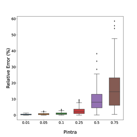
Figure 3: Relative error of SBM for different $P_{intra}$ with $3000$ nodes, $200$ components and $P_{inter}=0.0001$

$P_{intra}$	focal set size	# edges	MSE
0.01	2382	655	0.052
0.05	1788	1536	0.093
0.1	1349	2588	0.124
0.25	636	5673	0.351
0.5	271	10872	1.193
0.75	200	16157	2.120

Table 2: Mean squared error (MSE) for our Gnn-DML approach on graph generated using a stochastic block model with $3000$ units and $200$ blocks for different values of intra-block tie probabilities, represented as $P_{intra}$.

12.2 Coverage Study

In our investigation, we performed a comprehensive coverage analysis leveraging the closed-form formula for calculating variance and confidence intervals as detailed in Section 5.2. This analysis involved applying our proposed methodology across multiple executions—specifically, 100 iterations—on each dataset under consideration. For each iteration, we computed confidence intervals and assessed the frequency at which the true value of the target parameter fell within these intervals. This measure of frequency serves as a critical indicator of the reliability and precision of our methodology in capturing the parameter of interest across varied datasets. The results are presented in table 3.

Dataset	$\theta$	$\alpha$
Cora	100%	100%
Pubmed	100%	100%
Flickr	92%	52%

Table 3: The results of coverage study our approach across datasets over 100 trials with the 95% confidence interval

References

• Aronow and Samii, (2013) Aronow, P. M. and Samii, C. (2013). Estimating average causal effects under interference between units. arXiv: Statistics Theory.
• Athey et al., (2015) Athey, S., Eckles, D., and Imbens, G. W. (2015). Exact P-values for Network Interference. NBER Working Papers 21313, National Bureau of Economic Research, Inc.
• Attanasio et al., (2023) Attanasio, O., Kochar, A., Mahajan, A., and Surendra, V. (2023). Risk sharing, commitment constraints and self help groups. Technical report, National Bureau of Economic Research.