Order-One Rolling Shutter Cameras

Abstract.

Rolling shutter (RS) cameras dominate consumer and smartphone markets. Several methods for computing the absolute pose of RS cameras have appeared in the last 20 years, but the relative pose problem has not been fully solved yet. We provide a unified theory for the important class of order-one rolling shutter (RS₁) cameras. These cameras generalize the perspective projection to RS cameras, projecting a generic space point to exactly one image point via a rational map. We introduce a new back-projection RS camera model, characterize RS₁ cameras, construct explicit parameterizations of such cameras, and determine the image of a space line. We classify all minimal problems for solving the relative camera pose problem with linear RS₁ cameras and discover new practical cases. Finally, we show how the theory can be used to explain RS models previously used for absolute pose computation.

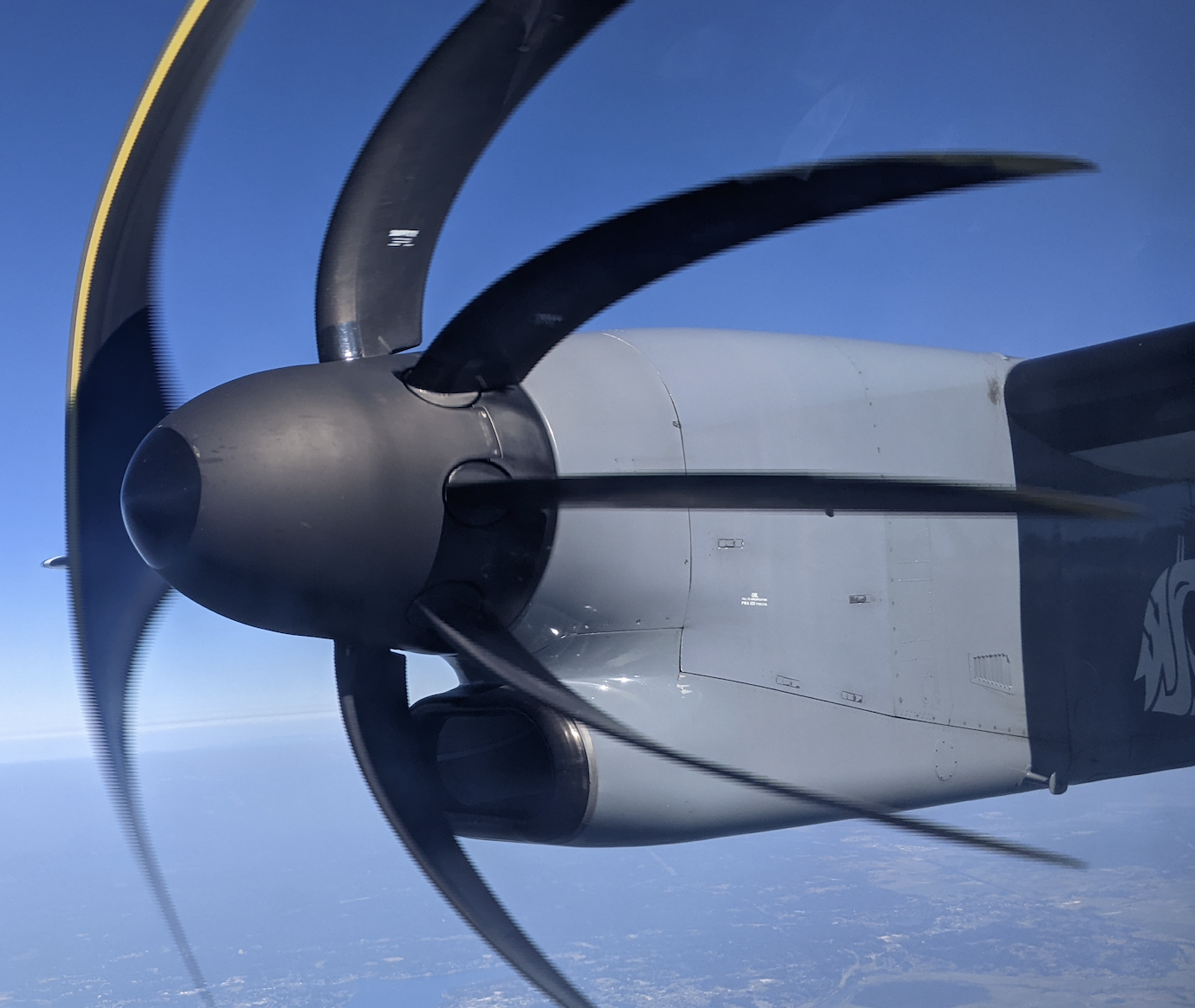
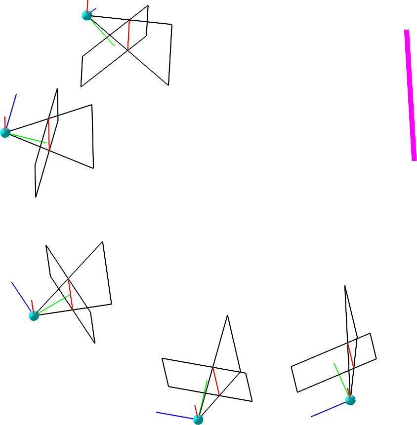
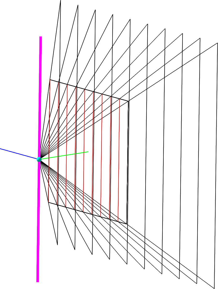
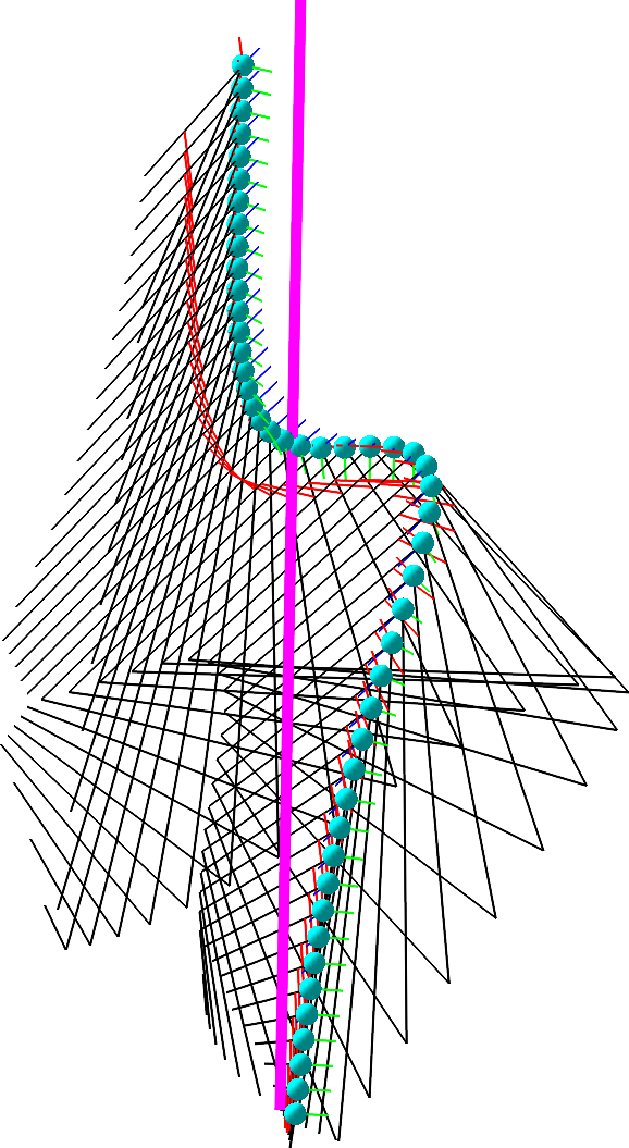
(a)	(b)	(c)	(d)

Figure 1. (a) General rolling shutter cameras see points in space multiple times (en.wikipedia.org/wiki/Rolling_shutter). (b) Order-one rolling shutter cameras see points in space exactly once. Their rolling planes intersect in a line. Examples are (c) perspective cameras, (d) some Straight-Cayley cameras moving on a twisted cubic.

1. Introduction

Rolling shutter cameras (RS) [1] dominate consumer and smartphone markets thanks to affordability, enhanced resolution, and rapid frame rates. Unlike global shutter cameras (GS), RS cameras capture images sequentially line-by-line, causing image distortions if the camera moves during capture (Fig. 1a). The distorted RS images do not match the geometry of GS cameras and thus are unsuitable for standard GS computer vision algorithms. Hence, a new theory and algorithms must be developed for RS cameras. Many partial results appeared in the last 20 years [2, 3, 4, 5, 6, 7, 8, 9, 10, 11, 12, 13, 14, 15, 16, 17, 18, 19, 20, 21, 22, 23, 24, 25, 26, 27, 28, 29, 30, 31]. Here, we provide a unified theory and analyze the important class of order-one RS cameras.

General RS cameras project a point in space into many image points (Fig. 1a). Perspective cameras project a point in space by a linear rational map to exactly one image point. Thus, it is natural to study a generalization of perspective cameras: RS cameras that project a point in space to exactly one image point via a rational map. We call these Order-one Rolling Shutter (RS₁) cameras.

1.1. Contribution and main results

We present a systematic study of RS and RS₁ cameras.

In Section 2, we introduce a new back-projection model of RS cameras that provides explicit parameterizations of RS camera-rays via a map $\Lambda$ (4) and of RS camera rolling planes via a map $\Sigma$ (2). Our model connects the geometry of rays in space with the image projection maps of RS cameras. The map $\Lambda$ assigns to every image point the ray in space that projects to the point. In general, there is no inverse map to $\Lambda$ for RS cameras that see space points several times.

RS₁ cameras are precisely those where such an inverse picture-taking map $\Phi$ exists and is rational. We analyze these maps in Section 3. We show (Theorem 4) that all rolling planes of an RS₁ camera intersect in a space line $K$. Furthermore, the rolling planes map $\Sigma$ of such a camera is birational and the camera center moves on a curve $\mathcal{C}$ that either equals $K$ or intersects $K$ in $\deg(\mathcal{C})-1$ points.

In Section 4, we construct explicit parameterizations of RS₁ cameras. Explicit parameterizations open a way to identify camera parameters from image measurements. We give the dimensions of several RS₁ parameter spaces needed to characterize minimal problems (Section 6). We analyze the interesting special cases of (1) constant rotation (Section 4.1) and (2) pure translation with a constant speed (Section 4.3), which were studied in [13] under the name linear RS cameras.

RS₁ cameras give rise to picture-taking maps $\Phi$. In Section 5, we give the degree of $\Phi$ for all parameterizations of RS₁ cameras from Section 4, Theorem 12, and show that the image of a line in space is a rational image curve of degree $\deg(\Phi)$ that passes through a special point at infinity $\deg(\Phi)-1$ many times. This means that the image of a space line contains precisely one further point at infinity. We use that point to simplify the camera relative pose minimal problems (Section 6).

In Section 6, we present all minimal problems for computing the relative poses of linear RS₁ cameras from correspondences between multiple images of points and lines (with potential incidences) under complete visibility assumptions [32]. We show that there are exactly 31 minimal problems for 2, 3, 4, and 5 cameras (Fig. 2). All these minimal problems are new. We also show that no minimal problems exist for a single camera and more than 5 cameras. For every minimal problem, we compute the number of solutions (degree). There are several practical minimal problems for two cameras: (i) Three problems with small degrees (28, 48, 60) and a small number of image features (e.g., 7 or 9 points, or 3 points + 2 lines) are suitable for constructing efficient symbolic-numeric minimal solvers [33, 34, 35]. (ii) Two important problems with 7 and 9 points have moderate degrees (140, 364) and thus are suitable for solving by optimized homotopy continuation [36, 32, 37]. Similarly, there is a practical problem for three cameras with degree 160. Minimal problems for more than three cameras are much harder and impractical unless they could be decomposed into simple problems [38]. This is an open problem for the future.

Section 7 shows when a practical “Straight-Cayley” (SC) RS camera model [20] produces RS₁ cameras. The SC model is important since it leads to tractable minimal RS camera absolute pose problems [20]. We provide explicit general constraints on the CS model and concrete examples. This demonstrates how the theory for RS₁ cameras developed in this paper can be used to understand existing practical RS camera models.

1.2. The most relevant previous work

[13] formulates the relative pose problems for two RS cameras for several RS models, but order-one cameras were not considered and camera order was not investigated. We show that general linear RS cameras have order two and that they have order one exactly when the motion line $\mathcal{C}$ is parallel to the camera projection plane. The uniform RS camera model of [13] uses the Rodrigues parameterization [39] of rotation, which is not algebraic. Hence, [13] replaces rotation matrices by their linearization to arrive at an approximate algebraic model. We use the Cayley rotation parameterization (17), which is algebraic, and we show when it produces RS₁ cameras. [13] observes that there is an 11-point minimal relative pose problem for two order-two linear RS cameras but does not present the solver. Instead, a rather impractical 20-point linear solver is suggested. We consider an RS₁ model and use all the algebraic constraints to get a solvable 9-point minimal relative RS₁ camera problem. We also classify all minimal problems for this model for arbitrarily many cameras (Fig. 2) and identify several practical RS camera relative pose problems.

[40, 20] developed efficient absolute pose minimal problems with the Straight-Cayley model. We show that the Straight-Cayley model is not only efficient but also very general and accounts for a large class of RS cameras, ranging from perspective cameras to many order-one cameras suitable for practical applications.

[41] studies linear congruences for modeling ray arrangements of generalized cameras [42, 43, 44]. It characterizes order-one congruences and together with its follow-up paper [45] introduces “photographic camera” projection maps that are rational. They study special two-slit cameras but do not relate the congruences and maps to RS cameras. We extend[41, 45] to real problems arising with RS cameras.

1.3. Concepts used in the main paper

We work with cameras that take pictures of points in projective $3$-space $\mathbb{P}^{3}$ and produce points in the projective image plane $\mathbb{P}^{2}$. We often identify planes $\Sigma$ in $\mathbb{P}^{3}$ with points $\Sigma^{\vee}$ in the dual space $(\mathbb{P}^{3})^{\ast}$. The Grassmannian $\mathrm{Gr}(1,\mathbb{P}^{3})$ is the set of lines in $\mathbb{P}^{3}$. For a line $L\in\mathrm{Gr}(1,\mathbb{P}^{3})$, we write $L^{\vee}\subset(\mathbb{P}^{3})^{\ast}$ for its dual line. The span of projective subspaces $X$ and $Y$ is denoted by $X\vee Y$. An algebraic variety is a solution set of polynomial equations. The Zariski closure of a set is the smallest algebraic variety containing the set. The degree of an algebraic curve $\mathcal{C}$ in $\mathbb{P}^{3}$ is the number of complex points in its intersection with a generic plane. We indicate rational functions, that are possibly not defined everywhere, via dashed arrows $\dashrightarrow$. A birational map is a rational function that is bijective onto its image almost everywhere (i.e., outside of a proper subvariety of the domain).

Additional concepts, definitions, lemmas, and the proofs are included in the SM.

2. Rolling shutter camera model

A rolling shutter camera arises from moving a perspective camera with center $C$ and projection plane $\Pi$ in the space $\mathbb{P}^{3}$ while scanning the projection plane $\Pi$ along a pencil $\mathcal{R}$ of (parallel) rolling image lines. Rolling lines capture the effect of the rolling shutter. In applications, $C$, $\Pi$ and lines $r\in\mathcal{R}$ are functions of time. However, typically, $\mathcal{R}$ is in one-to-one correspondence with a time interval. Thus, we use $r$ to parameterize the camera motion and write $C(r)$ and $\Pi(r)$.

Each rolling line $r\in\mathcal{R}$ generates a rolling plane $\Sigma(r)$ that is the preimage of $r$ for the perspective camera with center $C(r)$ and projection plane $\Pi(r)$. The points of $\Sigma(r)\subset\mathbb{P}^{3}$ are projected onto the rolling line $r\subset\mathbb{P}^{2}$ along the pencil $\mathcal{L}(r)$ of lines in $\Sigma(r)$ that pass through the center $C(r)$. The union $\mathcal{L}=\bigcup_{r\in\mathcal{R}}\mathcal{L}(r)$ of all pencils $\mathcal{L}(r)$ forms the set of rays of the rolling shutter camera.

To specify a rolling shutter camera model, we need to parameterize the pencil $\mathcal{R}$ of the rolling lines in $\Pi$ and couple it with a parameterization of the motion of the perspective camera in $\mathbb{P}^{3}$. We set the coordinate system in the plane $\mathbb{P}^{2}$ so that the rolling lines are parallel to the $y$-axis. The rolling-lines pencil $\mathcal{R}$ is then parameterized by the bijective morphism

(1) $$\rho:\mathbb{P}^{1}\longrightarrow\mathcal{R},\quad(v:t)\longmapsto(0:1:0)\vee(v:0:t)\equiv(-t:0:v)\in(\mathbb{P}^{2})^{*}.$$

Considering the calibrated scenario [46], the camera position and orientation are defined on the affine chart $\mathbb{R}^{1}$ where $t\neq 0$. They are described by $C(\tfrac{v}{t})\in\mathbb{R}^{3}$ and $R(\tfrac{v}{t})\in\mathrm{SO}(3)$. This gives the corresponding projection matrix $P(\tfrac{v}{t}):=R(\tfrac{v}{t})\,[I_{3}\mid-C(\tfrac{v}{t})]$ in $\mathbb{R}^{3\times 4}$ that represents a linear map $\mathbb{P}^{3}\dashrightarrow\mathbb{P}^{2}$. Now, we can take the preimages of the rolling lines in $\mathcal{R}$ and obtain rolling planes in $\mathbb{P}^{3}$:

(2) $$\begin{split}\Sigma^{\vee}:\mathbb{R}^{1}\longrightarrow(\mathbb{P}^{3})^{*},\quad\tfrac{v}{t}\longmapsto\Sigma(\tfrac{v}{t})^{\vee}=(1:0:-\tfrac{v}{t})\cdot P(\tfrac{v}{t}).\end{split}$$

Now the set $\mathcal{L}$ of camera rays is determined, as it is the union of the pencils $\mathcal{L}(\tfrac{v}{t}):=\{L\in\mathrm{Gr}(1,\mathbb{P}^{3})\mid C(\tfrac{v}{t})\in L\subset\Sigma(\tfrac{v}{t})\}$. A natural global parametrization of this union of pencils is given by taking preimages of image points on $r=\rho(\tfrac{v}{t}:1)$ under the projection matrix $P(\tfrac{v}{t})$. To parameterize the points on $r$, we intersect $r$ with another conveniently chosen set of lines, reflecting pixels on images. For that, we make the standard choice, using lines parallel to the $x$-axis:

$$\nu:\mathbb{P}^{1}\longrightarrow(\mathbb{P}^{2})^{*},\quad(u:s)\longmapsto(1:0:0)\vee(0:u:s)\equiv(0:-s:u)\in(\mathbb{P}^{2})^{*}.$$

An image point on the rolling line $r=\rho(v:t)$ is obtained by intersecting $r$ with the line $\nu(u:s)$, which is captured by the birational map

(3) $$\varphi:\mathbb{P}^{1}\times\mathbb{P}^{1}\dashrightarrow\mathbb{P}^{2},\quad((v:t),(u:s))\longmapsto(sv:ut:st).$$

This map is not defined at the point $((1:0),(1:0))$, where the lines $\rho(1:0)$ and $\nu(1:0)$ are both equal to the line at infinity. We obtain all camera rays in $\mathcal{L}$ by taking the preimages in $\mathbb{P}^{3}$ of the image points with affine coordinates $(\tfrac{u}{s},\tfrac{v}{t})$ under the projection matrix $P(\tfrac{v}{t})$ (see Section SM 1.1 for a derivation):

(4) $$\begin{split}\Lambda:\mathbb{R}^{1}\times\mathbb{R}^{1}\to\mathrm{Gr}(1,\mathbb{P}^{3}),\;(\tfrac{v}{t},\tfrac{u}{s})\mapsto\left[\!\!\begin{array}[]{cc}I_{3}\\ -C(\tfrac{v}{t})^{\top}\end{array}\!\!\right]\left[R(\tfrac{v}{t})^{\top}\left[\!\!\begin{array}[]{r}\tfrac{v}{t}\\ \tfrac{u}{s}\\ 1\end{array}\!\!\right]\right]_{\times}\!\!\!\![I_{3}\mid-C(\tfrac{v}{t})].\end{split}$$

Here, given a vector $V\in\mathbb{R}^{3}$, we write $[V]_{\times}$ for the skew-symmetric $3\times 3$ matrix that represents the linear map that takes the cross product with $V$. Then, $\Lambda(\tfrac{v}{t},\tfrac{u}{s})$ is a skew-symmetric $4\times 4$ matrix whose entries are the dual Plücker coordinates of the camera ray that the camera maps to the image point $(\tfrac{v}{t},\tfrac{u}{s})$, i.e., the $(i,j)$-th entry of $\Lambda(\tfrac{v}{t},\tfrac{u}{s})$ is the determinant of the submatrix with columns $(i,j)$ of the $2\times 4$ matrix whose two rows are $(0:1:-\tfrac{u}{s})\cdot P(\tfrac{v}{t})$ and $\Sigma(\tfrac{v}{t})^{\vee}$.

The set $\mathcal{L}$ of all camera rays captures most of the essential geometry of the camera, while its parametrization $\Lambda$ describes the concrete imaging process onto an actual picture plane [47]. Note that we used the term ‘camera rays’ for lines through the camera center, and not for actual rays in the sense of half-lines. This a good model for rolling shutter cameras with a view of less than 180 degrees. For more general modeling, we’d have to consider half-lines with orientation.

Remark 1.

$G:=\{[\begin{smallmatrix}R&t\\ 0&\alpha\end{smallmatrix}]\mid R\in\mathrm{SO}(3),t\in\mathbb{R}^{3},\alpha\in\mathbb{R}\setminus\{0\}\}$ is the scaled special Euclidean group on $\mathbb{R}^{3}$. It acts on the space of rolling shutter cameras. For a camera given by the projection-matrix map $P:\mathbb{R}^{1}\to\mathbb{R}^{3\times 4},\tfrac{v}{t}\mapsto P(\tfrac{v}{t})$ and a group element $g\in G$, the action is defined via

$$g.P:=\left(\mathbb{R}^{1}\to\mathbb{R}^{3\times 4},\;\tfrac{v}{t}\mapsto P(\tfrac{v}{t})\cdot g\right).$$

When acting simultaneously on cameras and the world points $X\in\mathbb{P}^{3}$ via $g.X:=g^{-1}\cdot X$, the imaging process stays invariant. Indeed, writing $g.\Lambda$ for the map (4) associated with the transformed projection $g.P=g.(R[I_{3}|-C])$, we have that the line $(g.\Lambda)(\tfrac{v}{t},\tfrac{u}{s})$ is the image of the line $\Lambda(\tfrac{v}{t},\tfrac{u}{s})$ under the $G$-action on $\mathbb{P}^{3}$. This means that 3D reconstruction using our camera model is only possible up to a proper rigid motion and a non-zero scale.

3. Order-one cameras

In this article, we analyze rolling shutter cameras that see a generic (i.e., sufficiently random) point in $3$-space exactly once, i.e., such that a generic space point appears exactly once on the image plane $\mathbb{P}^{2}$. For that to happen, two conditions need to be satisfied: First, for a generic point in $\mathbb{P}^{3}$, there has to be a unique camera ray in $\mathcal{L}$ passing through it. Second, the camera ray has to correspond to a unique point on the image plane via the map $\Lambda$. We classify all rolling shutter cameras satisfying those conditions, where we additionally impose the imaging process to be algebraic, i.e., we require $\Lambda$ to be a rational map.

The rationality of the map $\Lambda$ implies that both the rolling planes map $\Sigma$ and the center-movement map $C:\mathbb{R}^{1}\to\mathbb{R}^{3}$ are rational; see Lemma SM.1. In that case, the center locus $\mathcal{C}$, that is the Zariski closure in $\mathbb{P}^{3}$ of the image of $C$, is either a point or a rational curve. Moreover, the Zariski closure $\overline{\mathcal{L}}$ of the set $\mathcal{L}$ of camera rays inside the Grassmannian $\mathrm{Gr}(1,\mathbb{P}^{3})$ is a surface (or a one-dimensional pencil in the degenerate case when the center locus $\mathcal{C}$ is a single point and all rolling planes are equal); see Lemma SM.2. Such a surface in $\mathrm{Gr}(1,\mathbb{P}^{3})$ is classically called a line congruence [48]. An important invariance of such a congruence is its order. The order is the number of lines on the congruence that pass through a generic space point. Hence, we are interested in rolling shutter cameras whose associated congruence $\overline{\mathcal{L}}$ has order one.

Definition 2.

We say that a rolling shutter camera has order one if its associated congruence $\overline{\mathcal{L}}$ has order one and its parametrization $\Lambda$ is birational. We shortly write RS₁ camera for a rolling shutter camera of order one.

For RS₁ cameras, the image projection is a rational function $\Phi:\mathbb{P}^{3}\dashrightarrow\mathbb{P}^{2}$, which we can explicitly describe as follows: The congruence $\overline{\mathcal{L}}$ has order one if and only if there is a map $\Gamma:\mathbb{P}^{3}\dashrightarrow\overline{\mathcal{L}}$ from (a Zariski dense subset of) $\mathbb{P}^{3}$ to the camera rays that assigns to a visible point $X$ the unique ray that sees it. The map $\Lambda$ is birational if and only if it is rational and we can invert it, which means that the camera ray $\Gamma(X)$ corresponds to the unique image point $\Lambda^{-1}(\Gamma(X))$. Using the embedding $\mathbb{R}^{1}\times\mathbb{R}^{1}\subset\mathbb{P}^{1}\times\mathbb{P}^{1}$, we see that taking a picture of a generic space point $X\in\mathbb{P}^{3}$ yields an image point as follows:

(5) $$\begin{split}\Phi:\mathbb{P}^{3}\dashrightarrow\mathbb{P}^{2},\quad X\longmapsto\varphi(\Lambda^{-1}(\Gamma(X))).\end{split}$$

Example 3.

A familiar RS₁ camera is the static pinhole camera. Its congruence $\overline{\mathcal{L}}$ consists of all lines passing through the fixed camera center $C$. The map $\Gamma$ assigns to each space point $X\neq C$ the camera ray spanned by $C$ and $X$. That ray intersects the static projection plane $\Pi\cong\mathbb{P}^{2}$ in the unique point $\Phi(X)$.

Theorem 4.

Consider a rolling shutter camera whose congruence-parametriza- tion map $\Lambda$ is rational. The camera has order one if and only if the intersection of all rolling planes $\Sigma(\tfrac{v}{t})$ is a line $K$, the rolling planes map $\Sigma$ is birational, and its center locus $\mathcal{C}$ is one of the following:
I.   $\mathcal{C}$ is a rational curve that intersects the line $K$ in $\deg\mathcal{C}-1$ many points, or
II.  $\mathcal{C}=K$, or
III. $\mathcal{C}$ is a point on $K$.

Remark 5.

In type I, the points in the intersection $\mathcal{C}\cap K$ are counted with multiplicity. Also, the maps $\Sigma$ and $C$ determine each other: Whenever $C(\tfrac{v}{t})\notin K$, we have $\Sigma(\tfrac{v}{t})=K\vee C(\tfrac{v}{t})$. Conversely, every rolling plane $\Sigma(\tfrac{v}{t})$ meets $\mathcal{C}$ in $\deg\mathcal{C}$ many points (counted with multiplicity), out of which all but one lie on the line $K$. The remaining point is $C(\tfrac{v}{t})$. In particular, since $\Sigma$ is birational, so is $C$.

4. Building RS₁ cameras

Theorem 4 is constructive, meaning that we can use it to build – in theory – all RS₁ cameras. In the following, we describe the spaces of all RS₁ cameras of types I, II, and III. We start with type I. For that, we consider

$$\mathcal{H}_{d}:=\{(\mathcal{C},K)\mid\mathcal{C}\!\subset\!\mathbb{P}^{3}\text{ rational curve of degree }d,\,K\!\subset\!\mathbb{P}^{3}\text{ line},\,\#(K\cap\mathcal{C})=d-1\},$$

where $\#$ counts with multiplicities. We can explicitly pick elements in this parameter space as follows: Choose a line $K$. Rotate and translate such that $K$ becomes the $z$-axis $K^{\prime}:=(0:0:1:0)\vee(0:0:0:1)$. Every curve $\mathcal{C}^{\prime}$ with $(\mathcal{C}^{\prime},K^{\prime})\in\mathcal{H}_{d}$ is parametrized by $\mathbb{P}^{1}\dashrightarrow\mathbb{P}^{3},(v:t)\mapsto(vf(v:t):tf(v:t):g(v:t):h(v:t))$, where $f,g,h$ are homogeneous polynomials of degree $d-1,d,d$ [47, Eqn. (18)]. Reverse the translation and rotation to obtain $(\mathcal{C},K)\in\mathcal{H}_{d}$.

Picking elements in $\mathcal{H}_{d}$ allows us to parametrize all RS₁ cameras of type I. For that, let $H^{\infty}$ denote the plane at infinity $(0:0:0:1)^{\vee}\subseteq\mathbb{P}^{3}$. We denote the intersection of any variety $\mathcal{V}\subseteq\mathbb{P}^{3}$ with $H^{\infty}$ by $\mathcal{V}^{\infty}$. For any map $\Sigma^{\vee}:\mathbb{P}^{1}\dashrightarrow(\mathbb{P}^{3})^{*}$, we define $\Sigma^{\vee}_{\infty}(v:t)\in(H^{\infty})^{*}$ as the projection of $\Sigma^{\vee}(v:t)$ to $(H^{\infty})^{*}$. In the primal $\mathbb{P}^{3}$, this is the line that is the intersection of the planes $\Sigma(v:t)$ and $H^{\infty}$. Finally, for vectors $A,B$, we write $A\cdot B$ for the bilinear form $\sum_{i}A_{i}B_{i}$.

Proposition 6.

The RS₁ cameras of type I are in 4-to-1 correspondence with

$$\small\mathcal{P}_{I,d,\delta}:=\left\{\begin{array}[]{l}(K,\mathcal{C},\\ \Sigma^{\vee}_{\infty},\lambda)\end{array}\;\middle|\;\begin{array}[]{l}(\mathcal{C},K)\in\mathcal{H}_{d},\,\mathcal{C}^{\infty}\neq\mathcal{C},\,K^{\infty}\neq K,\,\lambda:\mathbb{P}^{1}\dashrightarrow K,\,\deg(\lambda)=\delta,\\ \Sigma^{\vee}_{\infty}:\mathbb{P}^{1}\dashrightarrow(K^{\infty})^{\vee},(v:t)\mapsto Av+Bt\text{ for some }A,B\text{ with }\\ A\cdot B=0\text{ and }A\cdot A=B\cdot B\end{array}\right\}.$$

The dimension of this parameter space is $\dim\mathcal{P}_{I,d,\delta}=3d+2\delta+7.$

Each element $(K,\mathcal{C},\Sigma^{\vee}_{\infty},\lambda)$ in $\mathcal{P}_{I,d,\delta}$ corresponds to four RS₁ cameras as follows: The rolling planes map $\Sigma$ of the cameras can be read off from the the map $\Sigma^{\vee}_{\infty}$ since each rolling plane $\Sigma(v:t)$ is the span of the line $\Sigma_{\infty}(v:t)$ with $K$. By Remark 5, the map $\Sigma$ determines uniquely the parametrization $C$ of the curve $\mathcal{C}$, i.e., the movement of the camera center. The camera rotation map $R:\mathbb{R}\to\mathrm{SO}(3)$ is fixed as follows: For $x\in\mathbb{R}$, $R(x)$ has three degrees of freedom. The first two are accounted for by the rolling plane $\Sigma(x)$. Here, we have to choose an orientation / sign of the normal vector of the plane $\Sigma(x)$, since this is not encoded in the projective map $\Sigma$. Finally, the map $\lambda:\mathbb{P}^{1}\dashrightarrow K$ chooses the unique point $\lambda(x)$ on $K$ that the projection matrix $P(x)$ maps to $(0:1:0)$, the intersection point of all rolling lines. Thus, $\lambda(x)$ fixes the third degree of freedom of $R(x)$, but its sign gives us again two choices. In summary, the two choices of orientation, that on $\Sigma$ and that on $\lambda$, give us four rotation maps $R:\mathbb{R}\to\mathrm{SO}(3)$.

Remark 7.

For every line, conic, or non-planar rational curve $\mathcal{C}$ of degree at most five, there is a RS₁ camera moving along $\mathcal{C}$. For a generic rational curve of degree at least six, there is no such camera.

Proposition 8.

The RS₁ cameras of type II are in 4-to-1 correspondence with

$$\small\mathcal{P}_{II,d,\delta}:=\left\{\begin{array}[]{l}(K,C,\\ \Sigma^{\vee}_{\infty},h,p)\end{array}\middle|\begin{array}[]{l}K\in\mathrm{Gr}(1,\mathbb{P}^{3}),\,K^{\infty}\neq K,\,C:\mathbb{P}^{1}\dashrightarrow K,\,\deg(C)=d,\\ \Sigma^{\vee}_{\infty}:\mathbb{P}^{1}\dashrightarrow(K^{\infty})^{\vee},(v:t)\mapsto Av+Bt\text{ for some }A,B\text{ with }\\ A\!\cdot\!B=0\text{ \& }A\!\cdot\!A=B\!\cdot\!B,\,(h,p)\in\mathbb{P}(\mathbb{R}[v,t]_{\delta}\times\mathbb{R}[v,t]_{\delta+d+1})\end{array}\right\}\!.$$

RS₁ cameras of type III are the special case when $d=0$ and the image of the constant map $C$ is not at infinity. Moreover, $\dim\mathcal{P}_{II,d,\delta}=3d+2\delta+8.$

An element $(K,C,\Sigma^{\vee}_{\infty},h,p)$ in $\mathcal{P}_{II,d,\delta}$ gives rise to four RS₁ cameras as follows: $C$ describes the movement of the camera center. As above, the map $\Sigma_{\infty}^{\vee}$ determines the rolling planes map $\Sigma$, which fixes (up to orientation) two degrees of freedom of each rotation $R(x)$ for $x\in\mathbb{R}$. To fix the third degree, we assume (by rotating and translating) that $K$ is the $z$-axis. Then, $C=(0:0:C_{3}:C_{0})$, where $C_{3},C_{0}$ are homogeneous of degree $d$, and $\Sigma^{\vee}=(\Sigma_{1}:\Sigma_{2}:0:0)$, where $\Sigma_{1},\Sigma_{2}$ are homogeneous linear forms. The polynomials $h,p$ define a map $\xi:\mathbb{P}^{1}\dashrightarrow\mathrm{Gr}(1,\mathbb{P}^{3})$ in Plücker coordinates: $(0:-h\Sigma_{2}C_{3}:-h\Sigma_{2}C_{0}:h\Sigma_{1}C_{3}:h\Sigma_{1}C_{0}:p)$. This map satisfies $C(v:t)\in\xi(v:t)\subseteq\Sigma(v:t)$ for all $(v:t)\in\mathbb{P}^{1}$ (see Lemma SM.15). It chooses the unique camera ray $\xi(x)$ that the projection matrix $P(x)$ maps to $(0:1:0)$. Thus, up to sign, $\xi(x)$ fixes $R(x)$. The two choices of orientation, that on $\Sigma$ and that on $\xi$, give us four rotation maps $R:\mathbb{R}\to\mathrm{SO}(3)$.

4.1. Constant rotation

In the special case when we know that a camera does not rotate, we can more easily check whether its order is one. In fact, the center-movement map $C$ is rational if and only if $\Lambda$ is rational (see (4) and Lemma SM.1), and the condition that all its rolling planes meet in a line implies all other conditions in Theorem 4.

Proposition 9.

A rolling shutter camera with constant rotation and rational center movement has order one if and only if the intersection of all its rolling planes is a line.

We denote the three rows of the constant rotation matrix $R\in\mathrm{SO}(3)$ by $w_{1},w_{2},w_{3}$. Then, we can write the rolling planes map (2) as $\Sigma:(v:t)\mapsto(w_{2}:0)\vee(vw_{1}+tw_{3}:0)\vee C(v:t)$. In particular, all rolling planes go through the point $(w_{2}:0)$. When the intersection of the rolling planes is a line $K$, then $(w_{2}:0)$ is the unique point of intersection of $K$ with the plane at infinity. (Otherwise, if $K$ were contained in that plane, then all rolling planes would be equal to that plane.) In particular, the line $K$ determines the second row of $R$ (up to sign) and the remaining rows of $R$ determine the rolling planes map as

(6) $$\Sigma:(v:t)\mapsto K\vee(vw_{1}+tw_{3}:0).$$

Hence, for constant rotation, the spaces of RS₁ cameras of types I–III are

$$\small\mathcal{P}_{I,d} :=\left\{(R,K,\mathcal{C})\;\middle|\;\begin{array}[]{l}R\in\mathrm{SO}(3)\text{ with second row }w_{2},\,K\in\mathrm{Gr}(1,\mathbb{P}^{3}),\\ K^{\infty}=(w_{2}:0),\,(\mathcal{C},K)\in\mathcal{H}_{d}\end{array}\right\},$$

$$\mathcal{P}_{II,d} :=\left\{(R,K,C)\;\middle|\;\begin{array}[]{l}R\in\mathrm{SO}(3)\text{ with second row }w_{2},\ K\in\mathrm{Gr}(1,\mathbb{P}^{3}),\\ K^{\infty}=(w_{2}:0),\,C:\mathbb{P}^{1}\dashrightarrow K,\,\deg(C)=d\end{array}\right\},$$

and $\mathcal{P}_{II,0}$ (with $\mathrm{im}(C)\neq K^{\infty}$) is the space of static pinhole cameras. Their dimensions are $\dim\mathcal{P}_{I,d}=3d+6$ and $\dim\mathcal{P}_{II,d}=2d+6$.

4.2. Moving along a line with constant speed

In many applications, where the camera moves along a line, it moves with approximately constant speed. Projectively, this means that the parameterization $C$ of the line $\mathcal{C}$ is birational with $C(1:0)=\mathcal{C}^{\infty}$. In the case of RS₁ cameras of type I, this means that $\Sigma(1:0)=K\vee\mathcal{C}^{\infty}$ is already determined by $K$ and $\mathcal{C}$, and cannot be freely chosen. Thus, the space of such RS₁ cameras is

$$\small\mathcal{P}^{\mathrm{cs}}_{I,1,\delta}:=\left\{\begin{array}[]{l}(K,\mathcal{C},\\ \Sigma^{\vee}_{\infty},\lambda)\end{array}\middle|\begin{array}[]{l}K,\mathcal{C}\in\mathrm{Gr}(1,\mathbb{P}^{3}),\,\mathcal{C}^{\infty}\neq\mathcal{C},\,K^{\infty}\neq K,\,K\cap\mathcal{C}=\emptyset,\\ \Sigma^{\vee}_{\infty}:\mathbb{P}^{1}\dashrightarrow(K^{\infty})^{\vee},(v:t)\mapsto Av+Bt,\text{ where }A\!=\!(K^{\infty}\!\vee\!\mathcal{C}^{\infty})^{\vee},\\ A\cdot B=0,A\cdot A=B\cdot B,\,\lambda:\mathbb{P}^{1}\dashrightarrow K,\,\deg(\lambda)=\delta\end{array}\right\}$$

The dimension of this space is one less than the space $\mathcal{P}_{I,1,\delta}$ without the constant-speed assumption, i.e., $\dim\mathcal{P}^{\mathrm{cs}}_{I,1,\delta}=2\delta+9$, since the birational map $\Sigma^{\vee}_{\infty}$ is already prescribed. In fact, over the reals, there are two such maps since the coefficient vector $B$ can be scaled by $-1$. Similarly, the space of RS₁ cameras of type II that move with constant speed is

$$\footnotesize\mathcal{P}^{\mathrm{cs}}_{II,1,\delta}\!:=\!\left\{\!\begin{array}[]{l}(K,C,\\ \Sigma^{\vee}_{\infty},h,p)\end{array}\middle|\begin{array}[]{l}K\!\in\!\mathrm{Gr}(1,\mathbb{P}^{3}),K^{\infty}\!\neq\!K,\,C:\mathbb{P}^{1}\dashrightarrow K\text{ birational},C(1\!:\!0)\!=\!K^{\infty},\\ \Sigma^{\infty}:\mathbb{P}^{1}\dashrightarrow(K^{\infty})^{\vee},(v:t)\mapsto Av+Bt\text{ for some }A,B\text{ with }\\ A\cdot B=0,A\cdot A=B\cdot B,\,(h,p)\in\mathbb{P}(\mathbb{R}[v,t]_{\delta}\times\mathbb{R}[v,t]_{\delta+2})\end{array}\right\}$$

and has dimension $\dim\mathcal{P}^{\mathrm{cs}}_{II,1,\delta}=2\delta+10$.

4.3. Linear RS₁ cameras

As in [13], we call a rolling shutter camera that does not rotate and moves along a line with constant speed a linear rolling shutter camera. Here, we describe such cameras of order one. Since, in type I, constant speed means that $\Sigma(1:0)=K\vee\mathcal{C}^{\infty}$, we see from (6) that the point $\mathcal{C}^{\infty}$ has to lie on the line in the plane at infinity that is spanned by the first two rows of the fixed rotation matrix $R$:

$$\mathcal{P}_{I,1}^{\mathrm{cs}}:=\left\{(R,K,\mathcal{C})\;\middle|\;\begin{array}[]{l}R=\left[\begin{smallmatrix}w_{1}\\ w_{2}\\ w_{3}\end{smallmatrix}\right]\in\mathrm{SO}(3),\,K\in\mathrm{Gr}(1,\mathbb{P}^{3}),\,K^{\infty}=(w_{2}:0),\\ \mathcal{C}\in\mathrm{Gr}(1,\mathbb{P}^{3}),\,K\cap\mathcal{C}=\emptyset,\,\mathcal{C}^{\infty}\in(w_{1}:0)\vee(w_{2}:0)\end{array}\right\}.$$

Since the rotation is constant, the embedded projection plane $\Pi(v:t)$ of the camera is only affected by parallel translation. It stays always parallel to the plane spanned by $w_{1}$, $w_{2}$ and the origin in $\mathbb{R}^{3}$. Projectively, this means that $\Pi(v:t)^{\infty}=(w_{1}:0)\vee(w_{2}:0)$ for all $(v:t)\in\mathbb{P}^{1}$. Hence, the last condition in the definition of $\mathcal{P}_{I,1}^{\mathrm{cs}}$ means that the line $\mathcal{C}$ has to be parallel to the projection plane $\Pi$. In particular, the projection plane does not change at all over time.

For linear RS₁ cameras of type II, we have analogously

$$\mathcal{P}_{II,1}^{\mathrm{cs}}:=\left\{(R,K,C)\;\middle|\begin{array}[]{l}R\in\mathrm{SO}(3)\text{ with second row }w_{2},\,K\in\mathrm{Gr}(1,\mathbb{P}^{3}),\\ K^{\infty}\!=\!(w_{2}:0),\,C:\mathbb{P}^{1}\dashrightarrow K\text{ birational},\,C(1:0)=K^{\infty}\end{array}\right\}.$$

The dimensions of these spaces are $\dim\mathcal{P}_{I,1}^{\mathrm{cs}}=3+2+3=8$ and $\dim\mathcal{P}_{II,1}^{\mathrm{cs}}=3+2+2=7$. The following proposition tells us how we can put $\mathcal{P}_{I,1}^{\mathrm{cs}}$ and $\mathcal{P}_{II,1}^{\mathrm{cs}}$ into a joint parameter space.

Proposition 10.

A linear rolling shutter camera (i.e., that moves with constant speed along a line $\mathcal{C}\subseteq\mathbb{P}^{3}$ and does not rotate) has order one if and only if the line $\mathcal{C}$ is parallel to the projection plane $\Pi$. If $\mathcal{C}$ is parallel to the rolling-shutter lines on $\Pi$, then the RS₁ camera is of type II. Otherwise, it is of type I.

The joint parameter space is

(10) $$\mathcal{P}^{\mathrm{cs}}_{1}:=\left\{(R,\mathcal{C},C)\;\middle|\;\begin{array}[]{l}R=\left[\begin{smallmatrix}w_{1}\\ w_{2}\\ w_{3}\end{smallmatrix}\right]\in\mathrm{SO}(3),\\ \mathcal{C}\in\mathrm{Gr}(1,\mathbb{P}^{3}),\,\mathcal{C}\neq\mathcal{C}^{\infty}\in(w_{1}:0)\vee(w_{2}:0),\\ C:\mathbb{P}^{1}\dashrightarrow\mathcal{C}\text{ birational},\,C(1:0)=\mathcal{C}^{\infty}\end{array}\right\}.$$

The parameters with $\mathcal{C}^{\infty}=(w_{2}:0)$ correspond to type-II cameras; the others to type-I cameras.

Remark 11.

A linear rolling shutter camera whose center moves on a line that is not parallel to the projection plane has order two.

5. The image of a line under a general $RS_{1}$ camera

RS₁ cameras view 3D points exactly once. So when they take an image of a 3D line, the image is an irreducible curve. However, that curve is typically not a line. The degree of that image curve is the degree of the picture-taking map $\Phi$ in (5).

Theorem 12.

The degree of $\Phi$ for a general RS₁ camera in the parameter spaces described above is

$$\begin{tabular}[]{c||c|c|c|c|c|c|c|c}&$\mathcal{P}_{I,d,\delta}$&$\mathcal{P}_{I,1,\delta}^{\mathrm{cs}}$&$\mathcal{P}_{II,d,\delta}$&$\mathcal{P}_{II,1,\delta}^{\mathrm{cs}}$&$\mathcal{P}_{I,d}$&$\mathcal{P}_{I,1}^{\mathrm{cs}}$&$\mathcal{P}_{II,d}$&$\mathcal{P}_{II,1}^{\mathrm{cs}}$\\ \hline\cr$\deg\Phi$&$2d\!+\!\delta\!+\!1$&$\delta+3$&$2d\!+\!\delta\!+\!2$&$\delta+4$&$d+1$&$2$&$d+1$&$2$\end{tabular}.$$

The image curve of a line under an RS₁ camera is not an arbitrary rational curve of the degree as prescribed in Theorem 12. In fact, they have a single singularity at the image point where all rolling lines meet.

Proposition 13.

Consider an RS₁ camera. For a general line $L$, its image $\Phi(L)$ is a curve with multiplicity $\deg(\Phi)-1$ at the point $(0:1:0)$.

6. Minimal problems of linear RS₁ cameras

The linear RS₁ cameras have been classified in Proposition 10. This section classifies the minimal problems of structure-from-motion from linear RS₁ cameras that observe points, lines, and their incidences. In this setting, structure-from-motion is the following 3D reconstruction problem:

Problem 14.

We have pictures $Y_{1},\dotsc,Y_{m}$ of a finite set $X$ of points and lines in space. The points and lines in $X$ satisfy some prescribed incidences. Each picture was taken by a linear RS₁ camera. Find the set $X$ and the camera parameters that produced the pictures.

Let $\mathcal{P}^{m}$ be the set of all $m$-tuples of camera parameters. We can take $\mathcal{P}^{m}=(\mathcal{P}_{1}^{\mathrm{cs}})^{m}$, where the latter parameter space is defined in (10).

We consider point-line arrangements in $3$-space consisting of $p$ points and $\ell$ lines whose incidences are encoded by an index set $\mathcal{I}\subset[p]\times[\ell]$. That $(i,j)\in\mathcal{I}$ means that the $i$-th point is contained in the $j$-th line. We model intersecting lines by requiring their point of intersection to be one of the $p$ points. We then write $\mathfrak{X}=\mathfrak{X}(p,\ell,\mathcal{I})$ for the variety of all $p$-tuples of points and $\ell$-tuples of lines in space that satisfy the incidences prescribed by $\mathcal{I}$.

By Theorem 12, a general linear RS₁ camera maps a general line in space to an image conic. The next lemma explains that the line at infinity on the image plane intersects each image conic at two points: one is $(0:1:0)$, the other depends only on the camera parameters.

Lemma 15.

Let $(R,\mathcal{C},C)\in\mathcal{P}_{1}^{cs}$ be of type I and let $(a:b:0)$ be such that $\mathcal{C}^{\infty}=(a:b:0)\cdot R$. Consider the associated picture-taking map $\Phi\colon\mathbb{P}^{3}\dashrightarrow\mathbb{P}^{2}$ and a line $L\subset\mathbb{P}^{3}$. Then, we have:

• either $\overline{\Phi(L)}$ is a conic through the points $(0:1:0)$ and $(a:b:0)$,

• or $\overline{\Phi(L)}$ is the line through the points $(0:1:0)$ and $(a:b:0)$.

Hence, the camera maps a general point-line arrangement in $\mathfrak{X}$ to an arrangement in the image plane consisting of $p$ points and $\ell$ conics that satisfy the incidences $\mathcal{I}$ and such that all conics pass through the same two points at infinity, one of them being $(0:1:0)$. We write $\mathcal{Y}(p,\ell,\mathcal{I})$ for the variety of all such planar point-conic arrangements.

Note that, as soon as such an arrangement contains at least one conic, the point $(a:b:0)$ from Lemma 15 is known. It can be obtained from intersecting the conic with the line at infinity. If however only image points have been observed, then the point $(a:b:0)$ is a priori unknown. But we might have an oracle that has additional knowledge of camera parameters and provides us with that special point. Thus, we want to allow the possible knowledge of the point $(a:b:0)$ for each involved camera, without necessarily observing any image conics. We set the boolean value $p_{\infty}\in\{1,0\}$ according to whether we assume knowledge of the point $(a:b:0)$ or not. We write $\mathcal{Y}=\mathcal{Y}(p,\ell,\mathcal{I},p_{\infty})$ for the variety of all planar point-conic arrangements in $\mathcal{Y}(p,\ell,\mathcal{I})$ plus the point $(a:b:0)$ if $p_{\infty}=1$.

Problem 14 asks to compute the preimage of such a planar arrangement $y\in\mathcal{Y}$ under the rational joint-camera map $\mathcal{P}^{m}\times\mathfrak{X}\dashrightarrow\mathcal{Y}$. The scaled special Euclidean group $G$ from Remark 1 acts on the preimages of that map, so we rather consider the quotient on the domain and let $\Phi^{(m)}=\Phi^{(m)}(p,\ell,\mathcal{I})$ be the map

(11) $$\Phi^{(m)}:(\mathcal{P}^{m}\times\mathfrak{X})/G\dashrightarrow\mathcal{Y}.$$

Definition 16.

The Reconstruction Problem 14 is minimal if its solution set is non-empty and finite for generic input pictures. In that case, the number of complex solutions given a generic input is the degree of the minimal problem.

Theorem 17.

There are exactly 31 minimal problems for structure-from-motion with linear RS₁ cameras fully observing point-line arrangements, where either all or no given views know the special point $(a:b:0)$. They are shown in Fig. 2.

Figure 2. Illustration of all minimal problems as lines and points in $\mathbb{P}^{3}$. Each problem is encoded by 9 integers: The number $m$ of cameras, followed by its combinatorial signature (see Definition SM.19 ff.) with $p_{\infty}$ at the end. Points on dashed lines are known to be collinear in $\mathbb{P}^{3}$, but the image conics are not observed. Lower bounds for the degrees are shown below the sketches, see Remark SM.26. “$\ast$”: the maximum from different computational runs is shown (the actual number is close to the number shown). “$+$”: interrupted runs (the actual number is higher than the number shown).

7. Straight-Cayley cameras

In [20], the Straight-Cayley RS model with a constant speed translation in the camera coordinate system $\beta_{u}$ and Cayley rotation parameterization was used to set up a tractable minimal problem of RS absolute pose camera computation

(13) $$\lambda\left[\!\!\begin{array}[]{ccc}u&v&1\end{array}\!\!\right]^{\top} = R\left((u-u_{0})\,O_{\delta}\right)\,X_{\delta}+T_{\beta_{u}}+(u-u_{0})\,V_{\beta_{u}}$$

(17) $$R(c) = \frac{1}{d}\left[\!\!\begin{array}[]{ccc}1+c_{1}^{2}-c_{2}^{2}-c_{3}^{2}&2\,(c_{1}c_{2}-c_{3})&2\,(c_{1}c_{3}+c_{2})\\ 2\,(c_{1}c_{2}+c_{3})&1-c_{1}^{2}+c_{2}^{2}-c_{3}^{2}&2\,(c_{2}c_{3}-c_{1})\\ 2\,(c_{1}c_{3}-c_{2})&2\,(c_{2}c_{3}+c_{1})&1-c_{1}^{2}-c_{2}^{2}+c_{3}^{2}\end{array}\!\!\right]$$

$$d = 1+c_{1}^{2}+c_{2}^{2}+c_{3}^{2}$$

Here, we have depth $\lambda\in\mathbb{R}$, image coordinates $u,v\in\mathbb{R}$, the offset $u_{0}\in\mathbb{R}$, a rotation axis $O_{\delta}\in\mathbb{R}^{3}$ in the world coordinate system $\delta$, a 3D point $X_{\delta}\in\mathbb{R}^{3}$, a camera center $T_{\beta_{u}}\in\mathbb{R}^{3}$ for $u=u_{0}$ in the cameras coordinate system $\beta_{u}$, and a translation direction vector $V_{\beta_{u}}\in\mathbb{R}^{3}$. The translation velocity is given by $\|V_{\delta}\|=\|V_{\beta_{u}}\|$. The rotation angle $\theta$ of $R\left((u-u_{0})\,O_{\delta}\right)$ around the axis $o$ is determined by $(u-u_{0})\|O_{\delta}\|=\tan(\theta/2)$. Thus, for small angles, $\theta\simeq(u-u_{0})\|O_{\delta}\|/2$, and $\|O_{\delta}\|/2$ approximates the angular velocity of the rotation. We now show how the camera center moves in the world coordinate system $\delta$. We can write

$$\lambda\left[\!\!\begin{array}[]{ccc}u&v&1\end{array}\!\!\right]^{\top}=R\left((u-u_{0})\,O_{\delta}\right)\left(X_{\delta}-R\left((u-u_{0})\,O_{\delta}\right)^{\top}\left(-T_{\beta_{u}}-(u-u_{0})\,V_{\beta_{u}}\right)\right)$$

and thus we get the camera center $C$ in the world coordinate system $\delta$ as

(18) $$C_{\delta}(u)=-R\left((u-u_{0})\,O_{\delta}\right)^{\top}\left(T_{\beta_{u}}+(u-u_{0})\,V_{\beta_{u}}\right).$$

Proposition 18.

For generic choices of the parameters $O_{\delta},T_{\beta_{u}},V_{\beta_{u}}$, the curve $\mathcal{C}$ parametrized by $C_{\delta}$ is a twisted cubic curve and the RS camera has order four.

We are interested in understanding when such a camera has order one and falls into the setting of this paper. Recall that a necessary condition for order one is that all rolling planes intersect in a line.

Theorem 19.

All rolling planes intersect in a line if and only if the parameters $O_{\delta}=(o_{1},o_{2},o_{3})$, $T_{\beta_{u}}=(t_{1},t_{2},t_{3})$, $V_{\beta_{u}}=(v_{1},v_{2},v_{3})$ satisfy one of the following:

1. $v_{3}=0$, $o_{3}=0$, and $o_{2}=-1$; or

2. $v_{3}=0$, $o_{1}=0$, and $o_{2}^{2}+o_{3}^{2}+o_{2}=0$; or

3. $v_{3}=0$, $v_{1}=t_{3}$, $t_{1}=0$, $o_{1}=0$, and $o_{3}=0$.

In each case, the camera-center curve $\mathcal{C}$ is generically still a twisted cubic curve. In the first two cases, the RS camera has order one. In the third case, the RS camera has generically order three, and its order is one if and only if the parameters also satisfy the conditions in either 1. or 2.

Hence, the first two cases of Theorem 19 describe all RS₁ cameras in this setting.

Proposition 20.

For both cases of RS₁ cameras, the picture-taking map $\Phi$ is generically of degree four: it maps generic lines in space to quartic image curves.

We conclude this section with three examples from Theorem 19, depicted in Fig. 3.

Example 21 ($O_{\delta}\!=\!(1,-1,0),T_{\beta_{u}}\!=\!(0,0,1),V_{\beta_{u}}\!=\!(0,1,0)$).

This is an example of case 1 in Theorem 19. The camera center moves on the twisted cubic curve defined by

$$X_{1}X_{3}-X_{2}X_{3}+X_{2}X_{0}=0,\,2X_{2}^{2}+X_{3}^{2}+X_{3}X_{0}=0,\,2X_{1}X_{2}+X_{3}^{2}-X_{0}^{2}=0.$$

The line $K$, which is the intersection of all rolling planes, is defined by $X_{1}=0$ and $X_{3}=X_{0}$. It intersects the twisted cubic $\mathcal{C}$ at two complex conjugated points. The picture-taking map $\Phi:\mathbb{P}^{3}\dashrightarrow\mathbb{P}^{2}$ sends $(X_{1}:X_{2}:X_{3}:X_{0})$ to

$$\left(\begin{array}[]{c}{-2X_{1}^{2}X_{2}X_{3}-X_{1}X_{3}^{3}+2X_{1}^{2}X_{2}X_{0}+X_{1}X_{3}^{2}X_{0}+X_{1}X_{3}X_{0}^{2}-X_{1}X_{0}^{3}}\\ {-2X_{1}^{3}X_{3}\!-\!2X_{1}X_{3}^{3}\!+\!X_{2}X_{3}^{3}\!+\!3X_{1}X_{3}^{2}X_{0}\!-\!3X_{2}X_{3}^{2}X_{0}\!+\!3X_{2}X_{3}X_{0}^{2}\!-\!X_{1}X_{0}^{3}\!-\!X_{2}X_{0}^{3}}\\ 2X_{1}X_{2}X_{3}^{2}+X_{3}^{4}-4X_{1}X_{2}X_{3}X_{0}-2X_{3}^{3}X_{0}+2X_{1}X_{2}X_{0}^{2}+2X_{3}X_{0}^{3}-X_{0}^{4}\end{array}\right).$$

Example 22 ($O_{\delta}\!=\!(0,-\tfrac{1}{2},\tfrac{1}{2}),T_{\beta_{u}}\!=\!(0,0,1),V_{\beta_{u}}\!=\!(0,1,0)$).

This is an example of case 2 in Theorem 19. The camera center moves on the twisted cubic curve defined by

$$X_{1}X_{2}\!-\!X_{1}X_{3}\!-\!X_{1}X_{0}\!+\!2X_{3}X_{0}\!+\!2X_{0}^{2}=0=X_{1}^{2}\!+\!2X_{2}X_{3}\!+\!2X_{2}X_{0}\!-\!2X_{3}X_{0}\!-\!2X_{0}^{2},$$

$$X_{2}^{2}-X_{2}X_{3}-X_{1}X_{0}-2X_{2}X_{0}+X_{3}X_{0}+X_{0}^{2}=0.$$

The line $K$, the intersection of all rolling planes, is defined by $X_{1}=0$, $X_{2}=X_{0}$. It meets the twisted cubic $\mathcal{C}$ at the points $(0:0:1:0)$ and $(0:1:-1:1)$. The picture-taking map $\Phi:\mathbb{P}^{3}\dashrightarrow\mathbb{P}^{2}$ sends $(X_{1}:X_{2}:X_{3}:1)$ to

$$\left(\begin{array}[]{c}{-X_{1}^{3}X_{2}\!-\!2X_{1}X_{2}^{2}X_{3}\!+\!X_{1}^{3}\!-\!2X_{1}X_{2}^{2}\!+\!4X_{1}X_{2}X_{3}\!+\!4X_{1}X_{2}\!-\!2X_{1}X_{3}\!-\!2X_{1}}\\ {2X_{1}^{2}X_{2}^{2}\!+\!2X_{2}^{4}\!-\!X_{1}^{2}X_{2}X_{3}\!-\!X_{1}^{3}\!-\!4X_{1}^{2}X_{2}\!-\!2X_{1}X_{2}^{2}\!-\!6X_{2}^{3}\!+\!X_{1}^{2}X_{3}\!+\!2X_{1}^{2}\!+\!4X_{1}X_{2}\!+\!6X_{2}^{2}\!-\!2X_{1}\!-\!2X_{2}}\\ {X_{1}^{2}X_{2}^{2}\!+\!2X_{2}^{3}X_{3}\!-\!2X_{1}^{2}X_{2}\!+\!2X_{2}^{3}\!-\!6X_{2}^{2}X_{3}\!+\!X_{1}^{2}\!-\!6X_{2}^{2}\!+\!6X_{2}X_{3}\!+\!6X_{2}\!-\!2X_{3}\!-\!2}\end{array}\right).$$

Example 23 ($O_{\delta}\!=\!(0,1,0),T_{\beta_{u}}\!=\!(0,0,1),V_{\beta_{u}}\!=\!(1,1,0)$).

This is an example of case 3 in Theorem 19. The camera center moves on the twisted cubic curve defined by

$$X_{2}X_{3}\!+\!X_{1}X_{0}\!-\!2X_{2}X_{0}=0,\,X_{1}X_{2}\!+\!X_{2}^{2}\!-\!X_{3}X_{0}\!-\!X_{0}^{2}=0,\,X_{1}^{2}\!-\!X_{2}^{2}\!+\!X_{3}^{2}\!-\!X_{0}^{2}=0.$$

The line $K$, which is the intersection of all rolling planes, is defined by $X_{1}=0$ and $X_{3}=0$. It does not meet the twisted cubic curve $\mathcal{C}$.

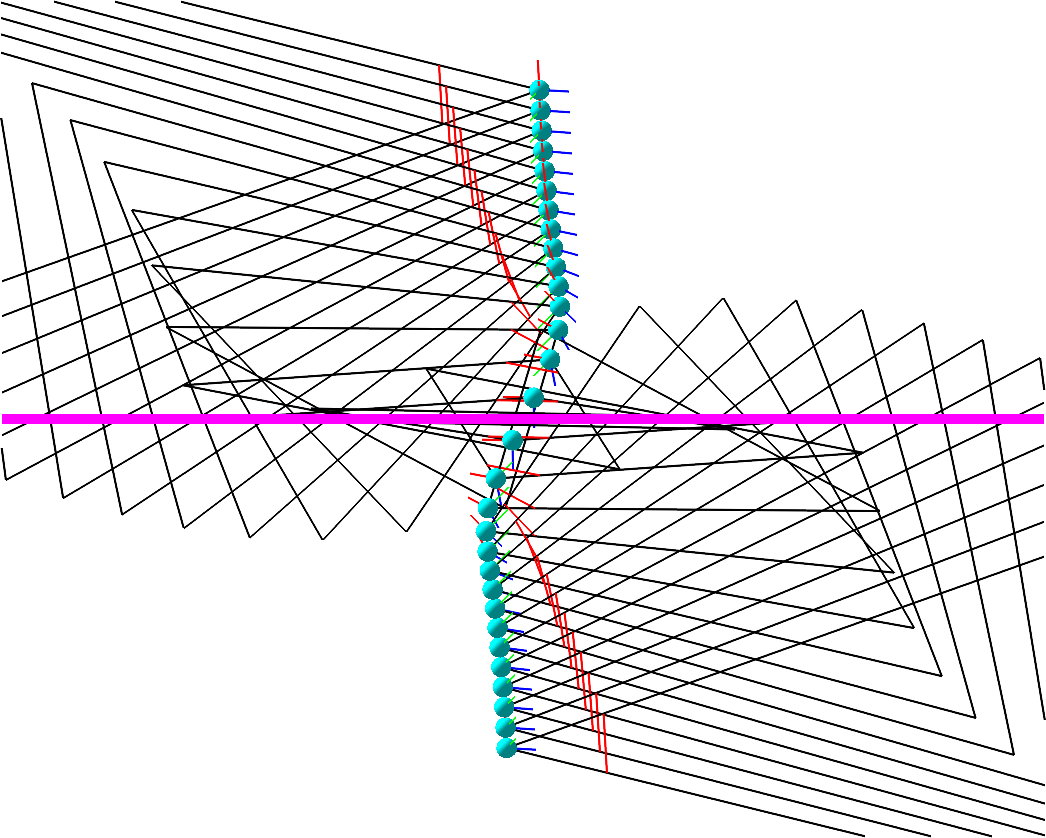
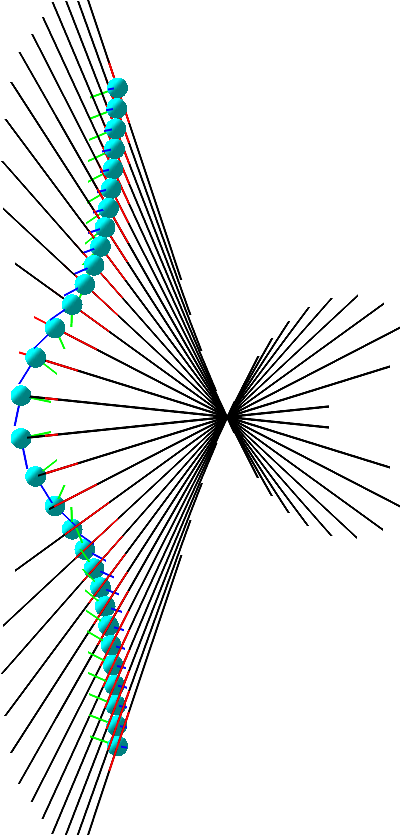
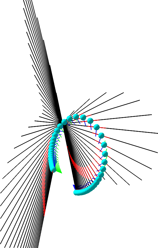
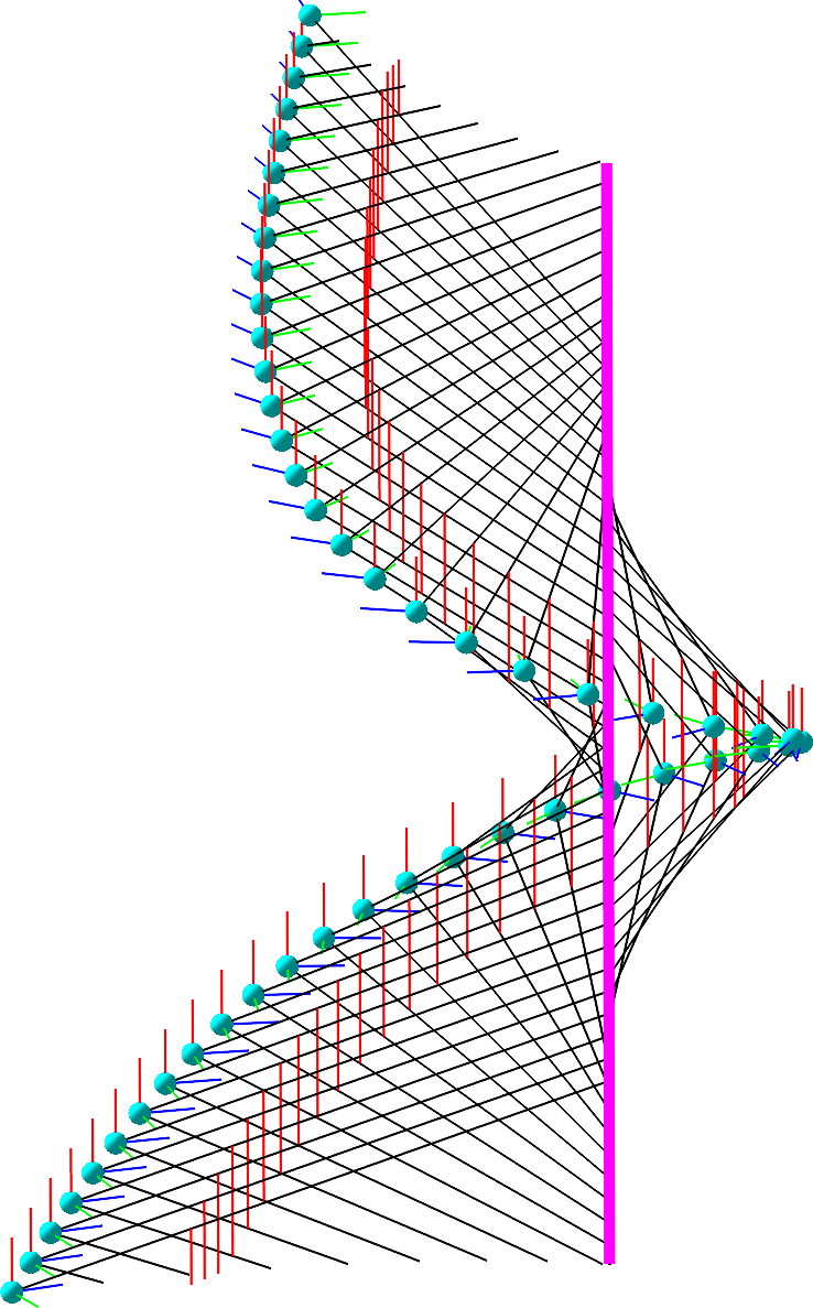
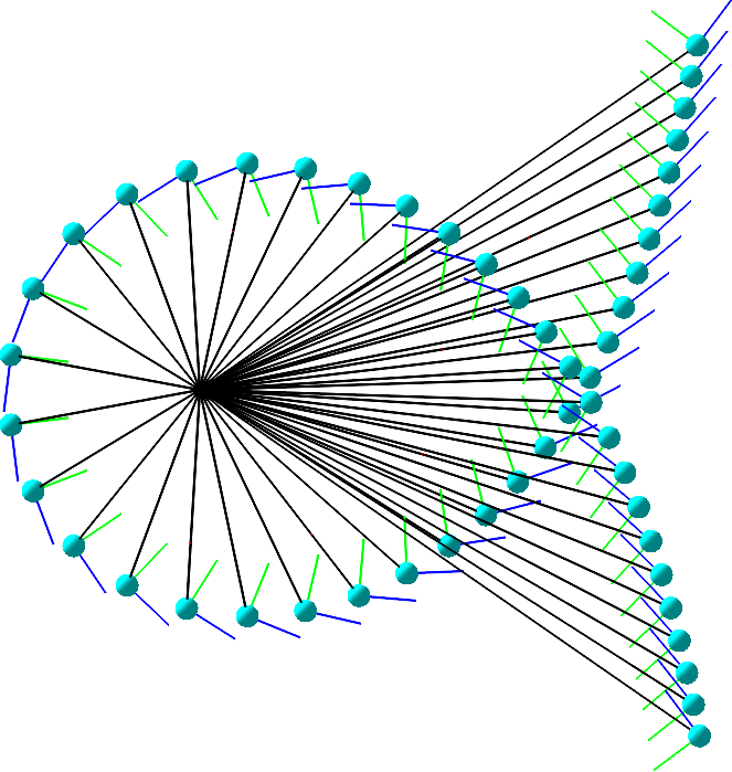
(a)	(b)	(c)

Figure 3. (a) Example 21, (b) Example 22, (c) Example 23. The camera center ${{\color[rgb]{0,1,1}C}}$ (cyan) moves along a twisted cubic curve $\mathcal{C}$. The rolling planes $\Sigma$ (black) intersect in a line ${{\color[rgb]{1,0,1}K}}$ (magenta). See Appendix SM 2 for larger figures and more details.

8. Conclusion

We provided a new model of RS cameras and characterized RS₁ cameras whose picture-taking process is encoded in a rational map. We described parameter spaces of RS₁ cameras and how images of lines taken by such cameras look. We classified all point-line minimal problems for linear RS₁ cameras and discovered new problems with small numbers of solutions and image features. In future work, we plan to implement and test the practicality of those new minimal solvers. Also, for the found minimal problems with higher degrees, we plan to investigate whether they can be decomposed into smaller problems via monodromy groups [49]. We further plan to classify the minimal relative pose problems for the Straight-Cayley RS model to exhibit whether this model is not only practical for absolute, but also relative pose. Finally, we will analyze higher-order cameras and the affect of the order on relative pose problems.

Here, we provide additional notation, definitions, concepts, technical lemmas and proofs of all results in the main paper. The code we used for computations is included as a pair of ancillary files. See readme.txt for how to use the code.

Appendix SM 1 Derivations and Proofs

Several of our proofs use projective duality of algebraic varieties. Hyperplanes in projective $n$-space $\mathbb{P}^{n}$ correspond to points of the dual space $(\mathbb{P}^{n})^{\ast}$. For a subvariety $V$ of $\mathbb{P}^{n}$, its dual variety $V^{\vee}$ is the Zariski closure inside $(\mathbb{P}^{n})^{\ast}$ of the set of hyperplanes that are tangent at some smooth point of $V$. Over the complex numbers, we have $(V^{\vee})^{\vee}=V$. More concretely, we have the following over $\mathbb{C}$: For a smooth point $p$ of $V$ and a smooth point $H^{\vee}$ of the dual variety $V^{\vee}$, the hyperplane $H$ is tangent to $V$ at the point $p$ if and only if the hyperplane $p^{\vee}$ is tangent to $V^{\vee}$ at the point $H^{\vee}$.

SM 1.1. Derivation of $\Lambda$ map

The camera ray through an image point results from intersecting backprojected planes of the image lines $\rho(v:t)$ and $\nu(u:s)$:

$$\Lambda:\qquad\mathbb{P}^{1}\times\mathbb{P}^{1} \,\dashrightarrow\mathrm{Gr}(1,\mathbb{P}^{3})^{*},$$

$$((u:s),(v:t)) \longmapsto[-t,0,v]\,R(v:t)\,[I_{3}\mid-C(v:t)]\wedge[0,-s,u]\,R(v:t)\,[I_{3}\mid-C(v:t)],$$

$$\longmapsto\left[\!\!\begin{array}[]{cc}I_{3}\\ -C(v:t)^{\top}\end{array}\!\!\right]R(v:t)^{\top}\left[\!\!\begin{array}[]{rrr}0{}&-st&ut\\ st&0{}&-sv\\ -ut&sv&0{}\end{array}\!\!\right]R(v:t)[I_{3}\mid-C(v:t)],$$

$$\longmapsto\left[\!\!\begin{array}[]{cc}I_{3}\\ -C(v:t)^{\top}\end{array}\!\!\right]R(v:t)^{\top}\left[\left[\!\!\begin{array}[]{r}sv\\ ut\\ st\end{array}\!\!\right]\right]_{\times}R(v:t)\,[I_{3}\mid-C(v:t)],$$

$$\longmapsto\left[\!\!\begin{array}[]{cc}I_{3}\\ -C(v:t)^{\top}\end{array}\!\!\right]\left[R(v:t)^{\top}\left[\!\!\begin{array}[]{r}sv\\ ut\\ st\end{array}\!\!\right]\right]_{\times}[I_{3}\mid-C(v:t)].$$

SM 1.2. Classifying RS₁ cameras

In this section, we prove Theorem 4. We assume throughout this section that the map $\Lambda$ is rational.

Lemma SM.1.

If the map $\Lambda$ is rational, so are the maps $C$ and $\Sigma^{\vee}$.

Proof.

Consider $(v:t)\in\mathbb{P}^{1}$ general. Then, the plane $\Sigma(v:t)^{\vee}$ is the equation of the Zariski closure of $\bigcup_{(u:s)\in\mathbb{P}^{1}}\Lambda((v:t),(u:s))$, which is the span of $\Lambda((v:t),(1:0))$ and $\Lambda((v:t),(0:1))$. This shows that $\Sigma^{\vee}$ is a rational map. Similarly, we see that $C$ is rational by observing that $C(v:t)$ is the intersection of $\Lambda((v:t),(1:0))$ and $\Lambda((v:t),(0:1))$. ∎

We start with showing that our unions of pencils of lines are indeed congruences, i.e., surfaces the Grassmannian $\mathrm{Gr}(1,\mathbb{P}^{3})$.

Lemma SM.2.

Let $X\subseteq\mathbb{P}^{3}\times(\mathbb{P}^{3})^{*}$ be an irreducible curve. For $(C,\Sigma^{\vee})\in X$, consider the pencil $\mathcal{L}(C,\Sigma)\coloneqq\{\xi\in\mathrm{Gr}(1,\mathbb{P}^{3})\mid C\in\xi\subseteq\Sigma\}$. Then the set $\mathcal{L}_{X}\coloneqq\bigcup_{(C,\Sigma^{\vee})\in X}\mathcal{L}(C,\Sigma)$ has dimension two.

Proof.

Let $\mathcal{V}\subseteq X\times\mathcal{L}_{X}$ be the incidence variety of elements $(C,\Sigma^{\vee},\xi)$ such that $\xi\in\mathcal{L}(C,\Sigma)$. Since all fibers over $X$ of $\mathcal{V}$ are one-dimensional, the variety $\mathcal{V}$ is two-dimensional. It remains to show that the generic fiber of $\mathcal{V}$ over $\mathcal{L}_{X}$ is zero-dimensional. Pick a general $\xi\in\mathcal{L}_{X}$ and let $\mathcal{C}$ be the image of $X$ in $\mathbb{P}^{3}$. Then the set $\{C\in\mathcal{C}\mid\xi\in\mathcal{L}(C,\Sigma)\text{ for some }\Sigma\}=\xi\cap\mathcal{C}$ is finite because $\xi$ is general. Dually, if $\mathcal{S}$ denotes the image of $X$ in $(\mathbb{P}^{3})^{*}$, then the set $\{\Sigma^{\vee}\in\mathcal{S}\mid\xi\in\mathcal{L}(C,\Sigma)\text{ for some }C\}=\xi^{\vee}\cap\mathcal{S}$ is also finite. Thus, the fiber of $\mathcal{L}_{X}$ over $\xi$ is finite. ∎

A rolling shutter camera that does not move but rotates has (almost) always the order-one congruence $\overline{\mathcal{L}}$ that consists of all lines passing through the fixed center. The only exception is when the rotation cancels out the movement of the rolling line such that all rolling planes are the same plane, say $\Sigma$. In that case, the camera rays do not form a congruence, but only the pencil of lines that are contained in $\Sigma$ and pass through the camera center. Such a camera can only take pictures of the points in the fixed plane $\Sigma$.

Thus, to classify all rolling shutter cameras with an order-one congruence, we may assume that the camera is actually moving (and possibly rotating). In the following, we use the rolling image lines $r\in\mathcal{R}$ synonymously with our projective parameters $(v:t)\in\mathbb{P}^{1}$, via the identification $\rho$ in (1).

Theorem SM.3.

Consider a rolling shutter camera whose center moves along a rational curve $\mathcal{C}\subseteq\mathbb{P}^{3}$. The associated congruence $\overline{\mathcal{L}}$ has order one if and only if the intersection of all rolling planes $\Sigma(r)$ is a line $K$ that satisfies one of the following two conditions:
1) $K$ intersects the curve $\mathcal{C}$ in $\deg\mathcal{C}-1$ many points (counted with multiplicty), or
2) $K=\mathcal{C}$ and $\Sigma(r_{1})=\Sigma(r_{2})$ implies $C(r_{1})=C(r_{2})$ for all $r_{1},r_{2}\in\mathcal{R}$.

In order to prove this theorem, we make use of Kummer’s classication of order-one congruences according to their focal loci [50]. A focal point of an order-one congruence $\overline{\mathcal{L}}$ is a space point that lies on infinitely many lines on $\overline{\mathcal{L}}$. The focal locus of the congruence is the Zariski closure of its set of focal points. The following version of Kummer’s classification is due to De Poi [51].

Theorem SM.4.

A congruence ${\mathcal{L}}\subset\mathrm{Gr}(1,\mathbb{P}^{3})$ has order one if and only if it is one of the following:

1. $\mathcal{L}$ is the set of all lines passing through a fixed point $C\in\mathbb{P}^{3}$. Its only focal point is $C$.

2. $\mathcal{L}$ consists of all secant (and tangent) lines of a twisted cubic curve $\mathcal{C}\subset\mathbb{P}^{3}$. Its focal locus is $\mathcal{C}$.

3. $\mathcal{L}$ consists of all lines that meet both a rational curve $\mathcal{C}\subset\mathbb{P}^{3}$ and a line $K\subset\mathbb{P}^{3}$ that intersects the curve $\mathcal{C}$ in $\deg\mathcal{C}-1$ many points (counted with multiplicity). Its focal locus is $\mathcal{C}\cup K$.

4. There is a line $K\subset\mathbb{P}^{3}$ and a dominant morphism $\sigma:K^{\vee}\to K$ such that $\mathcal{L}=\bigcup_{\Sigma^{\vee}\in K^{\vee}}\{\xi\in\mathrm{Gr}(1,\mathbb{P}^{3})\mid\sigma(\Sigma^{\vee})\in\xi\subset\Sigma\}$. Its focal locus is $K$.

Order-one congruences of type i are associated with rolling shutter cameras that stand still (but possibly rotate).

Lemma SM.5.

The congruence $\overline{\mathcal{L}}$ associated with a rolling shutter camera cannot be of type ii.

Proof.

The congruence is a union of pencils; in fact, ${\mathcal{L}}=\bigcup_{r\in\mathcal{R}}\mathcal{L}(r)$, where $\mathcal{L}(r)=\{\xi\in\mathrm{Gr}(1,\mathbb{P}^{3})\mid C(r)\in\xi\subset\Sigma(r)\}$. In particular, its focal locus contains the curve $\mathcal{C}$ along which the camera center moves. If the congruence $\overline{\mathcal{L}}$ were of type ii, the curve $\mathcal{C}$ would be a twisted cubic. However, any rolling plane $\Sigma(r)$ intersects the curve $\mathcal{C}$ in the camera center $C(r)$ and at most two other points, meaning that the generic line in $\mathcal{L}(r)$ is not a secant of $\mathcal{C}$. ∎

Remark SM.6.

The congruence associated with a rolling shutter camera has order zero if and only if all rolling planes are the same plane. This is because the set of points seen by the camera is the union of all rolling planes, which is a connected surface that contains a plane. When the congruence has order zero and all rolling planes are the same, the congruence consists of all lines in that plane and the camera moves along a rational curve in that plane.

Proof of Theorem SM.3.

We start by observing that the set of camera rays $\mathcal{L}$ of a moving rolling shutter camera is always two-dimensional by Lemma SM.2. Moreover, the focal locus of the congruence $\overline{\mathcal{L}}$ contains the curve $\mathcal{C}$ that describes the movement of the camera center. In particular, $\mathcal{L}$ cannot be of type i. Hence, by Theorem SM.4 and Lemma SM.5, the congruence $\overline{\mathcal{L}}$ has order one if and only if it is of type iii or iv.

We start by assuming that the congruence is of type iii. By considering the focal locus, we find that the rational curve from iii coincides with the camera movement curve $\mathcal{C}$. Since $\mathcal{L}$ is the union of the pencils $\mathcal{L}(r)=\{\xi\in\mathrm{Gr}(1,\mathbb{P}^{3})\mid C(r)\in\xi\subset\Sigma(r)\}$ and every of its lines has to meet a fixed line $K$, every rolling plane $\Sigma(r)$ has to contain $K$. The rolling planes cannot all be the same, because otherwise the congruence $\overline{\mathcal{L}}$ would consist of all lines in that plane, which is a congruence of order zero. Therefore, the intersection of the rolling planes is exactly the line $K$, and we are in type 1) of Theorem SM.3. Conversely, given a rolling shutter camera of type 1), the generic rolling plane $\Sigma(r)$ is the span of the center $C(r)$ with the line $K$, and thus $\overline{\mathcal{L}}$ is of type iii.

If the congruence $\overline{\mathcal{L}}$ is of type iv, the camera moves along a line $\mathcal{C}=K$. This line is the focal locus of $\overline{\mathcal{L}}$ and thus coincides with the line given in iv. We claim that every rolling plane $\Sigma(r)$ contains that line $K$. To see that, we assume for contradiction that one of the rolling planes $\Sigma(r)$ intersects $K$ in a single point, namely $C(r)$. Now, consider an arbitrary plane $\Sigma$ containing $K$ (i.e., $\Sigma^{\vee}\in K^{\vee}$). The intersection $\Sigma\cap\Sigma(r)$ is a line $\xi$ passing through the center $C(r)$. Thus, the line $\xi$ is on the pencil $\mathcal{L}(r)\subset\mathcal{L}$. Since $\Sigma$ is the unique plane that contains both $\xi$ and $K$, the expression of $\mathcal{L}$ in type iv of Theorem SM.4 shows that $\sigma(\Sigma^{\vee})\in\xi$, which implies that $\sigma(\Sigma^{\vee})=C(r)$. In other words, the map $\sigma:K^{\vee}\to K$ is constant with image $C(r)$, which contradicts its dominance. Hence, we have shown that the rolling planes intersect in the line $K$ (as before, they cannot all be equal, since otherwise the congruence would have order zero). Moreover, we have for any rolling plane $\Sigma(r)$ that $\sigma(\Sigma(r)^{\vee})=C(r)$, and we are in type 2) of Theorem SM.3. Conversely, for a rolling shutter camera of type 2), we have that $K^{\vee}$ consists of all rolling planes and the map $\sigma:K^{\vee}\to K,\Sigma(r)^{\vee}\mapsto C(r)$ is dominant since the camera is moving. Thus, $\mathcal{L}=\bigcup_{r\in\mathcal{R}}\mathcal{L}(r)$ is of type iv. ∎

To classify all RS₁ cameras, it remains to analyze when the congruence parametrization map $\Lambda$ is birational.

Lemma SM.7.

The map $\Lambda$ is birational if and only if, for a generic $\xi\in\mathcal{L}$, there is a unique $r\in\mathcal{R}$ such that $\xi\in\mathcal{L}(r)$.

Proof.

$\Lambda$ is birational if and only if, for a generic $\xi\in\mathcal{L}$, there are unique parameters $((v:t),(u:s))$ whose image under $\Lambda$ is $\mathcal{L}$. Recall that the morphism $\rho$ in (1) identifies the parameters $(v:t)\in\mathbb{P}^{1}$ with $r\in\mathcal{R}$. Hence, the birationality of $\Lambda$ implies for $\xi\in\mathcal{L}$ the existence of a unique $r\in\mathcal{R}$ with $\xi\in\mathcal{L}(r)$. Conversely, if a generic $\xi\in\mathcal{L}$ uniquely determines the pencil $\mathcal{L}(r)$ that contains it, then $\xi$ is uniquely picked in that pencil via the parameters $(u:s)$, i.e., $\Lambda$ is birational. ∎

Proposition SM.8.

Consider a rolling shutter camera whose associated congruence $\overline{\mathcal{L}}$ has order zero. The map $\Lambda$ is birational if and only if the camera moves on a line $\mathcal{C}$ and the center map $C:\mathcal{R}\dashrightarrow\mathcal{C}$ is birational.

Proof.

As in Remark SM.6, all rolling planes are the same plane, say $\Sigma$. The congruence is the family of all lines contained in $\Sigma$ and the camera moves along a rational plane curve $\mathcal{C}\subset\Sigma$. By Lemma SM.7, the map $\Lambda$ is birational if and only if, for a generic line $\xi\subset\Sigma$, there is a unique $r\in\mathcal{R}$ such that $C(r)\in\xi$. The latter means that the generic line $\xi$ intersects the plane curve $\mathcal{C}$ in a single point (i.e., $\deg\mathcal{C}=1$) and that $C$ is a birational map. ∎

Proposition SM.9.

Consider a rolling shutter camera that does not move (but possibly rotates). The map $\Lambda$ is birational if and only if the intersection of all rolling planes is a line $K$ and the rolling planes map $\Sigma$ is birational.

Proof.

The congruence is the family of lines passing through the fixed camera center $C\in\mathbb{P}^{3}$. Hence, this situation is projectively dual to the setting in Proposition SM.8. In particular, when considering the rolling planes $\Sigma(r)$ as points $\Sigma(r)^{\vee}$ in $(\mathbb{P}^{3})^{*}$, they form a curve in the plane $C^{\vee}\subset(\mathbb{P}^{3})^{*}$. As in the proof of Proposition SM.8, the birationality of $\Lambda$ means that that plane curve is a line (namely $K^{\vee}$) with a rational parametrization via the rolling planes map $\Sigma^{\vee}$. ∎

Theorem SM.10.

Consider a moving rolling shutter camera with a congruence $\overline{\mathcal{L}}$ of positive order. The map $\Lambda$ is birational if and only if the map $\mathcal{R}\dashrightarrow\mathbb{P}^{3}\times(\mathbb{P}^{3})^{*},r\mapsto(C(r),\Sigma(r)^{\vee})$ that parametrizes the pencils $\mathcal{L}(r)$ is birational. In particular, the birationality of $C:\mathcal{R}\dashrightarrow\mathcal{C}$ implies that $\Lambda$ is birational.

Proof.

The pairs $(C(r),\Sigma(r)^{\vee})$ trace a curve in $\mathbb{P}^{3}\times(\mathbb{P}^{3})^{*}$, which we denote by $\mathcal{D}$.

Let $\Lambda$ be birational and let $X$ be the set of pairs $(C(r),\Sigma(r)^{\vee})\in\mathcal{D}$ such that there is some $r^{\prime}\neq r$ with $(C(r),\Sigma(r)^{\vee})=(C(r^{\prime}),\Sigma(r^{\prime})^{\vee})$. The set $X$ has either dimension zero or it has dimension one. In the former case, we are done since a generic element of $\mathcal{D}$ will have a unique pre-image $r$. In the latter case, the union $\bigcup_{(C(r),\Sigma(r)^{\vee})\in X}\mathcal{L}(r)\subseteq\mathcal{L}$ is dense by Lemma SM.2, contradicting Lemma SM.7.

Now, we assume that the map $\mathcal{R}\dashrightarrow\mathcal{D}$ is birational. Then, by Lemma SM.7, it is enough to show that, for a generic $\xi\in\mathcal{L}$, there is a unique pair $(C,\Sigma^{\vee})\in\mathcal{D}$ such that $C\in\xi\subset\Sigma$. To prove this, we consider a generic line $\xi\in\mathcal{L}$ on the congruence and assume for contradiction that there are two distinct pairs $(C_{1},\Sigma_{1}^{\vee}),(C_{2},\Sigma_{2}^{\vee})\in\mathcal{D}$ such that $C_{i}\in\xi\subset\Sigma_{i}$ for $i=1,2$. We distinguish two cases.

First, if $C_{1}\neq C_{2}$, the generic line $\xi$ is a secant line of the curve $\mathcal{C}$ traced by the camera centers. Hence, the congruence $\overline{\mathcal{L}}$ is the family of secant lines of $\mathcal{C}$. In particular, all the lines $\xi^{\prime}$ in the pencil $C_{1}\in\xi^{\prime}\subset\Sigma_{1}$ have to be secants of $\mathcal{C}$, which is only possible if $\mathcal{C}$ is a plane curve contained in $\Sigma_{1}$. Since the same applies to the pencil given by $(C_{2},\Sigma_{2})$, we see in particular that $\Sigma_{1}=\Sigma_{2}$ (otherwise, the curve $\mathcal{C}$ would be the unique line in their intersection, but then its secants would not form a line congruence). However, the congruence $\overline{\mathcal{L}}$ is now simply the family of lines contained in the plane $\Sigma_{1}$, which has order zero; a contradiction to the assumptions in Theorem SM.10.

Second, if $C_{1}=C_{2}$, then we have necessarily that $\Sigma_{1}\neq\Sigma_{2}$. This case is projectively dual to the first case. In particular, the rolling planes $\Sigma(r)$ trace a curve in the plane $C_{1}^{\vee}\subset(\mathbb{P}^{3})^{*}$ and the dual congruence $\overline{\mathcal{L}}^{\vee}\subset\mathrm{Gr}(1,(\mathbb{P}^{3})^{*})$ is the family of secant lines of that plane curve. Hence, $\overline{\mathcal{L}}^{\vee}$ consists of all lines in the plane $C_{1}^{\vee}$, and $\overline{\mathcal{L}}$ consists of all lines passing through the center $C_{1}$. However, as observed at the beginning of the proof of Theorem SM.3, the latter is not possible for a moving camera. ∎

We obtain the following corollary for order one cameras.

Corollary SM.11.

Consider a moving rolling shutter camera whose associated congruence $\overline{\mathcal{L}}$ has order one. The map $\Lambda$ is birational if and only if the rolling planes map $\Sigma^{\vee}$ is birational.

Proof.

Clearly, if the map $\Sigma^{\vee}$ is birational, then the map $r\mapsto(C(r),\Sigma(r)^{\vee})$ is birational, and we can apply Theorem SM.10 to see that $\Lambda$ is birational. For the converse direction, the same statement implies that it is enough to show that the birationality of $r\mapsto(C(r),\Sigma(r)^{\vee})$ implies that $\Sigma^{\vee}$ is birational. To prove this, we consider the two cases of order-one congruences described in Theorem SM.3 separatly. In case 2), any rolling plane $\Sigma(r)$ determines the corresponding camera center $C(r)$, and then the birationality of $r\mapsto(C(r),\Sigma(r)^{\vee})$ ensures that there is a unique parameter $r$.

In case 1), a generic rolling plane $\Sigma(r)$ intersects the curve $\mathcal{C}$ is $\deg\mathcal{C}$ many points (counted with multiplicity). All except one of those points lie on the line $K$. The remaining point is the camera center $C(r)$, which is thus uniquely determined by $\Sigma(r)$. As above, the birationality of $r\mapsto(C(r),\Sigma(r)^{\vee})$ ensures that the parameter $r$ is unique. As a side note, a generic camera center $C(r)$ determines uniquely the corresponding rolling plane: $\Sigma(r)=C(r)\vee K$. Therefore, the birationality of the rolling planes map $\Sigma^{\vee}$ is equivalent to the birationality of the center map $C$. This also proves Remark 5. ∎

Proof of Theorem 4.

If the camera does not move, then $\mathcal{C}$ is a point. The associated congruence consists of all lines passing through that point and has order one. Hence, the camera has order one if and only if the map $\Lambda$ is birational. By Proposition SM.9, the latter is equivalent to the conditions in Theorem 4. The point $\mathcal{C}$ has to lie on the line $K$ since each rolling plane has to contain both $\mathcal{C}$ and $K$ and there is a one-dimensional family of such planes.

If the camera moves, then $\mathcal{C}$ is a rational curve. The camera has order one if and only if the conditions in Theorem SM.3 and Corollary SM.11 are satisfied. Note that the birationality of the map $\Sigma^{\vee}$ implies that every rolling plane $\Sigma(r)$ uniquely determines the parameter $r$ and thus also the corresponding camera center $C(r)$. Hence, the birationality of $\Sigma^{\vee}$ ensures that the cases 1) and 2) in Theorem SM.3 are equivalent to the types I and II in Theorem 4. ∎

SM 1.3. Camera Spaces

In this section, we prove Propositions 6 and 8.

Lemma SM.12.

The dimension of $\mathcal{H}_{d}$ is $3d+5$. For every line, conic, or nondegenerate rational curve $\mathcal{C}$ of degree at most five, there is a line $K$ such that $(\mathcal{C},K)\in\mathcal{H}_{\deg\mathcal{C}}$. For $d\geq 6$, the locus of rational degree-$d$ curves $\mathcal{C}$ that admit a line $K$ with $(\mathcal{C},K)\in\mathcal{H}_{d}$ is a low-dimensional subset of the locus of all rational degree-$d$ curves.

Proof of Lemma SM.12.

For curves $\mathcal{C}$ of degree at most two, there are clearly many such lines $K$. For curves $\mathcal{C}$ of degree at least three, the existence of such a line $K$ requires the curve $\mathcal{C}$ to be nondegenerate, i.e., not contained in any plane (otherwise, every secant line would automatically intersect the curve in $\deg\mathcal{C}$ many points). Every nondegenerate cubic curve has a two-dimensional family of secant lines $K$. It is a classical fact that every nondegenerate rational quartic curve has a one-dimensional family of trisecant lines $K$ (see e.g. [52]) and that every nondegenerate rational quintic curve has a quadrisecant line $K$ (in fact, typically a unique one; see [53, Remark 2.16]). Together with the fact that the locus of all rational degree-$d$ space curves has dimension $4d$, this discussion proves the first two assertions of Lemma SM.12 for $d\leq 5$.

For $d>5$, the locus $\mathcal{H}^{\prime}_{d}$ of rational curves in $\mathbb{P}^{3}$ of degree $d$ that intersect some line at $d-1$ or $d$ many points has dimension $3d+5<4d$ [53, Lem. 2.13]. Moreover, for the general curve in $\mathcal{H}^{\prime}_{d}$ (with $d\geq 5$), there is a unique line meeting the curve in $d-1$ points (and not $d$ points) [53, Thm. 2.15 & Rem. 2.16].∎

Lemma SM.12 implies Remark 7, i.e., that almost any rational curve of degree $d\leq 5$ can be the center locus of a RS₁ camera of type I, while only special curves are allowed when $d\geq 6$. Next, we determine which birational maps $\Sigma^{\vee}:\mathbb{P}^{1}\dashrightarrow K^{\vee}$ are allowed. The following lemma applies to all three types of RS₁ cameras, and uses the notation introduced in the paragraph before Proposition 6.

Lemma SM.13.

Let $C:\mathbb{P}^{1}\dashrightarrow\mathbb{P}^{3}$ be a rational map defined over $\mathbb{R}$ and let $\mathcal{C}$ be the complex Zariski closure of its image. Let $K\subseteq\mathbb{P}^{3}$ be a line and let $\Sigma^{\vee}:\mathbb{P}^{1}\dashrightarrow K^{\vee}$ be a birational map, both defined over $\mathbb{R}$, such that, for all $(v:t)\in\mathbb{P}^{1}$, the plane $\Sigma(v:t)$ contains the point $C(v:t)$. Assume that $\mathcal{C}\not\subseteq H^{\infty}$ and that $\mathcal{C}$ and $K$ are related as in Type I, II, or III of Theorem 4.

Then, the following are equivalent:

1. There exists an RS₁ camera of type I, II, or III with distinguished line $K$, center-movement map $C$, and rolling planes map $\Sigma^{\vee}$.

2. $K^{\infty}$ is a point and on its dual line $(K^{\infty})^{\vee}\subseteq(H^{\infty})^{*}$, there are points $A,B\in(K^{\infty})^{\vee}$ such that $A\cdot B=0$, $A\cdot A=B\cdot B$, and the map $\Sigma^{\vee}_{\infty}:\mathbb{P}^{1}\dashrightarrow(H^{\infty})^{*}$ is $\Sigma^{\vee}_{\infty}(v:t)=Av+Bt$.

Proof.

$(a)\Rightarrow(b)$: We begin by assuming that $C$, $K$, and $\Sigma^{\vee}$ are part of an RS₁ camera. In particular, the birational map $\Sigma^{\vee}$ is of the form (2). Thus, $\Sigma_{\infty}^{\vee}(x)=(1:0:-x)\cdot R(x)$ for $x\in\mathbb{R}$. The rotation matrix $R(x)$ preserves norms. So, after fixing a scaling for the rational map $\Sigma_{\infty}^{\vee}$, the former equation implies

(19) $$\frac{\Sigma_{\infty}^{\vee}(x)}{\|\Sigma_{\infty}^{\vee}(x)\|}=\frac{1}{\sqrt{1+x^{2}}}(1,0,-x)\cdot R(x).$$

For general $x\in\mathbb{R}$, the projection matrix $P(x)$ maps the whole plane $\Sigma(x)$ onto the rolling line $\rho(x:1)$. In particular, exactly one camera ray $\xi(x)\subseteq\Sigma(x)$ passing through $C(x)$ will be mapped by $P(x)$ to $(0:1:0)^{\top}$. Since $(0:1:0)=\varphi((x:1),(1:0))$, the homogenization of the map $\Lambda$ becomes well-defined at $((x:1),(1:0))$ and we see that $\xi(x)=\Lambda((x:1),(1:0))$. In particular, $\xi$ is a rational map.

Thus, $\omega(x)\coloneqq\xi_{\infty}(x)$ also defines a rational map. Since $P(x)\omega(x)=(0:1:0)^{\top}$, after fixing a scaling for the rational map $\omega$, we have

(20) $$R(x)\cdot\frac{\tilde{\omega}(x)^{\top}}{\|\tilde{\omega}(x)\|}=(0,1,0)^{\top},\quad\text{ where }\tilde{\omega}(x):=\left([I_{3}\mid-C(x)]\,\omega(x)\right)^{\top}.$$

Since $\omega(x)$ is of the form $(\omega_{1}:\omega_{2}:\omega_{3}:0)^{\top}$, the point $\tilde{\omega}(x)$ is simply $(\omega_{1}:\omega_{2}:\omega_{3})\in\mathbb{P}^{2}$. Equations (19) and (20) uniquely determine the rotation matrix $R(x)$. Indeed,

(21) $$R(x)=\left[\begin{matrix}\dfrac{1}{\sqrt{1+x^{2}}}&0&\dfrac{x}{\sqrt{1+x^{2}}}\\[15.0pt] 0&1&0\\[10.0pt] -\dfrac{x}{\sqrt{1+x^{2}}}&0&\dfrac{1}{\sqrt{1+x^{2}}}\end{matrix}\right]\cdot\left[\begin{matrix}\dfrac{\Sigma_{\infty}^{\vee}(x)}{\|\Sigma_{\infty}^{\vee}(x)\|}\\[15.0pt] \dfrac{\tilde{\omega}(x)}{\|\tilde{\omega}(x)\|}\\[15.0pt] \dfrac{\Sigma_{\infty}^{\vee}(x)\times\tilde{\omega}(x)}{\|\Sigma_{\infty}^{\vee}(x)\|\cdot\|\tilde{\omega}(x)\|}\end{matrix}\right].$$

For $x,y\in\mathbb{R}$, we may now compute $\Lambda_{\infty}(x,y)$, the intersection of the camera ray parametrized by $(x,y)$ with the plane $H^{\infty}$. The point $\Lambda_{\infty}(x,y)$ is the intersection of the lines represented by

$$(1:0:-x)\cdot R(x)=\Sigma_{\infty}^{\vee}(x)\quad\text{and}\quad(0:1:-y)\cdot R(x)\quad\text{in }(H^{\infty})^{*}.$$

We compute

$$\Lambda_{\infty}(x,y) =\Sigma^{\vee}_{\infty}(x)\times\left((0:1:-y)\cdot R(x)\right)$$

$$=\Sigma^{\vee}_{\infty}(x)\times\left(\frac{\tilde{\omega}(x)}{\|\tilde{\omega}(x)\|}-y\cdot\left(-\frac{x}{\sqrt{1+x^{2}}}\cdot\frac{\Sigma^{\vee}_{\infty}(x)}{\|\Sigma^{\vee}_{\infty}(x)\|}+\frac{1}{\sqrt{1+x^{2}}}\cdot\frac{\Sigma^{\vee}_{\infty}(x)\times\tilde{\omega}(x)}{\|\Sigma^{\vee}_{\infty}(x)\|\cdot\|\tilde{\omega}(x)\|}\right)\right)$$

(22) $$=\frac{\Sigma^{\vee}_{\infty}(x)\times\tilde{\omega}(x)}{\|\tilde{\omega}(x)\|}+\frac{y}{\sqrt{1+x^{2}}}\cdot\frac{\|\Sigma^{\vee}_{\infty}(x)\|}{\|\tilde{\omega}(x)\|}\cdot\tilde{\omega}(x).$$

The latter expression can be scaled to a rational function since $\Lambda$ is a rational map. Since the first term of $\|\tilde{\omega}(x)\|\cdot\Lambda_{\infty}(x,y)$ (which is $\Sigma^{\vee}_{\infty}(x)\times\tilde{\omega}(x)$) is already rational, the function $\|\tilde{\omega}(x)\|\cdot\Lambda_{\infty}(x,y)$ can only be scaled to a rational function if its second term ${y}\cdot\|\Sigma^{\vee}_{\infty}(x)\|\cdot\tilde{\omega}(x)/{\sqrt{1+x^{2}}}$ is rational as well. This means that ${\|\Sigma^{\vee}_{\infty}(x)\|}/{\sqrt{1+x^{2}}}$ is rational, which is equivalent to $\sqrt{1+x^{2}}\cdot\|\Sigma^{\vee}_{\infty}(x)\|$ being rational. For the affine linear map $\Sigma^{\vee}_{\infty}$ this means that $(1+x^{2})\cdot(\Sigma^{\vee}_{\infty}(x)\cdot\Sigma^{\vee}_{\infty}(x))=Q(x)^{2}$ for some quadratic polynomial $Q$. Since $K\subseteq\Sigma(x)$ for all $x$, we can write $\Sigma^{\vee}_{\infty}(x)=Ax+B$ for some $A,B\in(K^{\infty})^{\vee}$, and so a direct computation (e.g., with Macaulay2) reveals that the existence of $Q$ is equivalent to the conditions $A\cdot B=0$ and $A\cdot A=B\cdot B$.

Since the entries of $A$ and $B$ are real numbers, these two conditions imply that $A$ and $B$ are not scalar multiples of each other. Thus, the map $\Sigma^{\vee}_{\infty}$ is not constant, which implies that $K$ is not contained in $H^{\infty}$ (otherwise we would have $\Sigma^{\vee}_{\infty}(x)=K^{\vee}$ for all $x$).

$(b)\Rightarrow(a)$: We are given the data of $K$, $C$, and $\Sigma^{\vee}$, and need to find an RS₁ camera that conforms to these. First, the type of our camera (I, II, or III) is readable from $K$ and $\mathcal{C}$. Second, the rotation map $R$ must be determined. Third, the map $\Lambda$ defined in (4) has to be rational.

We define a map $\omega:\mathbb{P}^{1}\dashrightarrow H^{\infty}$ such that the line $\xi(x)$ spanned by $\omega(x)$ and $C(x)$ will be sent to $(0:1:0)$ by the camera. Fix any line $\ell$ at infinity and set $\omega(x)\coloneqq\Sigma(x)\wedge\ell$. Equation (21) now gives the definition of a rotation map $R$ that conforms to the given data.

Finally, since $\sqrt{1+x^{2}}\|\Sigma^{\vee}_{\infty}(x)\|=Q(x)$, we see from (22) that $\Lambda_{\infty}$ is a rational map (after multiplying by $\|\tilde{\omega}(\cdot)\|$). Therefore, also $\Lambda(x,y)=C(x)\vee\Lambda_{\infty}(x,y)$ is rational.∎

Lemma SM.13 gives an existence statement for RS₁ cameras of all types given the data $C$, $K$, $\Sigma^{\vee}$. That data determines uniquely the associated congruence $\overline{\mathcal{L}}$, but the camera rotation map $R:\mathbb{R}\to\mathrm{SO}(3)$ and the congruence parametrization $\Lambda$ are not yet fixed. In fact, there are many ways of defining a camera rotation map $R:\mathbb{R}\to\mathrm{SO}(3)$ that fits the data. For $x\in\mathbb{R}$, the orientation $R(x)$ has three degrees of freedom. The first two are accounted for, up to orientation, by the rolling plane $\Sigma(x)$. The third may be fixed, up to orientation, by the choice of which line $\xi(x)\subseteq\Sigma(x)$ passing through $C(x)$ is the camera ray that the projection matrix $P(x)$ maps to $(0:1:0)$, the intersection point of all rolling lines. Such a choice is expressed as a rational map $\xi:\mathbb{P}^{1}\dashrightarrow\mathrm{Gr}(1,\mathbb{P}^{3})$.

Lemma SM.14.

Let $(C,K,\Sigma^{\vee})$ satisfy the conditions from Lemma SM.13. The RS₁ cameras involving $C$, $K$, and $\Sigma^{\vee}$ are in 4-to-1 correspondence with rational maps $\xi:\mathbb{P}^{1}\dashrightarrow\mathrm{Gr}(1,\mathbb{P}^{3})$ satisfying $C(v:t)\in\xi(v:t)\subset\Sigma(v:t)$ for all $(v:t)\in\mathbb{P}^{1}$. The correspondence comes from the two choices of orientation, that on $\xi$ and that on $\Sigma$. Changing the orientation on $\xi$ does not change the picture-taking map $\Phi$. Changing the orientation on $\Sigma$ does change $\Phi$, from $(\Phi_{1}:\Phi_{2}:\Phi_{0})$ to $(\Phi_{1}:-\Phi_{2}:\Phi_{0})$.

Proof.

Given $(C,K,\Sigma^{\vee})$, we are interested in describing all possible orientation maps $R:\mathbb{R}\to\mathrm{SO}(3)$ that would conform to an RS₁ camera. As in the proof of Lemma SM.13, for every such camera, there is a rational map $\xi$ that assigns to every $x\in\mathbb{R}$ the camera ray that the projection matrix $P(x)$ maps to $(0:1:0)^{\top}$ (see paragraph under (19)). Conversely, any such map defines an orientation map $R:\mathbb{R}\to\mathrm{SO}(3)$ via (19) and (20) (with $\omega:=\xi_{\infty}$), after fixing a scaling for the rational maps $\Sigma_{\infty}^{\vee}$ and $\omega$. That means that $R(x)$ is actually only determined up to the signs of $\Sigma_{\infty}^{\vee}(x)$ and $\omega(x)$. Changing the sign of $\Sigma^{\vee}_{\infty}(x)$ would mean to use the unit normal vector of the rolling plane $\Sigma(x)$ that points in the opposite direction, i.e., a rotation around the ray $\xi(x)$ by $180^{\circ}$. Changing the sign of $\omega(x)$ amounts to a rotation around the normal vector of the plane $\Sigma(x)$ by $180^{\circ}$.

Finally, we have to analyze how these sign changes affect the picture-taking map $\Phi$. Recall from (5) that $\Phi$ is the composition of several maps. The map $\Gamma$ is not affected by the sign changes. Hence, it suffices to consider how $\Lambda\circ\varphi^{-1}$ is affected. In an affine chart, this map is spelled out in (22). On the one hand, changing the sign of $\Sigma^{\vee}_{\infty}(x)$, changes $\Lambda_{\infty}(x,y)$ in (22) to $-\Lambda_{\infty}(x,-y)$. On the other hand, changing the sign of $\omega(x)$, changes $\Lambda_{\infty}(x,y)$ in (22) simply to $-\Lambda_{\infty}(x,y)$. Combining this with the definition of the map $\varphi$ from (3) concludes the proof. ∎

We are now ready to prove Proposition 6.

Proof of Proposition 6.

With the lemmas established above, we can describe the parameter space of RS₁ cameras of type I, up to the above described choice of orientation. The first parameter is a line $K$. It is not allowed to lie at infinity due to Lemma SM.13. Second, we can choose any curve $\mathcal{C}$ of degree $d$, not at infinity, such that $(\mathcal{C},K)\in\mathcal{H}_{d}$. The third parameter is a map $\Sigma^{\vee}_{\infty}$ as in Lemma SM.13. The rolling planes map $\Sigma^{\vee}$ can be read off from the the map $\Sigma^{\vee}_{\infty}$ since each rolling plane $\Sigma(v:t)$ is the span of the line $\Sigma_{\infty}(v:t)$ with $K$. By Remark 5, the map $\Sigma$ determines uniquely the parametrization $C$ of the curve $\mathcal{C}$. Finally, we need to specify the map $\xi$. In Type I, for general $(v:t)\in\mathbb{P}^{1}$, the line $\xi(v:t)$ intersects the line $K$ at a point other than $C(v:t)$, giving rise to a rational map $\lambda:\mathbb{P}^{1}\dashrightarrow K$. Conversely, every such rational map $\lambda$ gives a camera-ray map $\xi\coloneqq\lambda\vee C$. Thus, the orientation map $R$ is specified, up to the $4:1$ relationship above, by $\lambda$. To summarize, the space of all type-I cameras is $\mathcal{P}_{I,d,\delta}$ in Proposition 6. There is a one-dimensional family of maps $\Sigma^{\vee}_{\infty}$ of the form described in Lemma SM.13, since choosing $A$ already determines $B$, up to sign. Hence, the camera space has dimension $\dim\mathcal{P}_{I,d,\delta}=(3d+5)+1+(2\delta+1)=3d+2\delta+7.$ ∎

Similarly, the parameters for an RS₁ camera of type II or III are the line $K$ (not at infinity), the center-movement map $C:\mathbb{P}^{1}\dashrightarrow K$ of degree $d\geq 0$, the map $\Sigma^{\vee}_{\infty}$ as in Lemma SM.13 which determines the rolling planes map $\Sigma^{\vee}$, and the map $\xi:\mathbb{P}^{1}\dashrightarrow\mathrm{Gr}(1,\mathbb{P}^{3})$ satisfying $C(v:t)\in\xi(v:t)$ and $\xi(v:t)\subseteq\Sigma(v:t)$ for all $(v:t)\in\mathbb{P}^{1}$. Once the data $(K,C,\Sigma^{\vee})$ is fixed, the following lemma shows that the map $\xi$ is determined by a pair of homogeneous polynomials $(h,p)$ of degrees $(\delta,\delta+d+1)$ for some $\delta\geq 0$.

We work in the following setting: we rotate and translate $K$ until it becomes the $z$-axis. Then, the center-movement map $C:\mathbb{P}^{1}\dashrightarrow\mathbb{P}^{3}$ takes the form $(0:0:C_{3}:C_{0})$, where $C_{3},C_{0}$ are homogeneous polynomials in two variables of degree $d\geq 0$. The rolling planes map $\Sigma^{\vee}:\mathbb{P}^{1}\dashrightarrow(\mathbb{P}^{3})^{*}$ takes the form $(\Sigma_{1}:\Sigma_{2}:0:0)$, where $\Sigma_{1},\Sigma_{2}$ are linear homogeneous polynomials in two variables. We represent the map $\xi:\mathbb{P}^{1}\dashrightarrow\mathrm{Gr}(1,\mathbb{P}^{3})$ by Plücker coordinates $(p_{12}:p_{13}:p_{10}:p_{23}:p_{20}:p_{30})$, where the $p_{ij}$ are homogeneous polynomials in two variables of arbitrary degree.

Lemma SM.15.

Assume that $K$ is the $z$-axis and consider maps $C:\mathbb{P}^{1}\dashrightarrow K$ and $\Sigma^{\vee}:\mathbb{P}^{1}\dashrightarrow K^{\vee}$. A map $\xi:\mathbb{P}^{1}\dashrightarrow\mathrm{Gr}(1,\mathbb{P}^{3})$ satisfies $C(v:t)\in\xi(v:t)$ and $\xi(v:t)\subseteq\Sigma(v:t)$ for all $(v:t)\in\mathbb{P}^{1}$ if and only its Plücker coordinates are

$$(p_{12}:p_{13}:p_{10}:p_{23}:p_{20}:p_{30})=(0:-h\Sigma_{2}C_{3}:-h\Sigma_{2}C_{0}:h\Sigma_{1}C_{3}:h\Sigma_{1}C_{0}:p_{30}),$$

where $h$ is a homogeneous polynomial in two variables.

Proof.

The degree-$d$ map $C$ is of the form $(0:0:C_{3}:C_{0})$. We can assume that $C_{3}$ and $C_{0}$ share no common factor, as otherwise we could make $d$ smaller. Since the birational map $\Sigma=(\Sigma_{1}:\Sigma_{2}:0:0)$ is not constant, we note the same for $\Sigma_{1}$ and $\Sigma_{2}$.

The condition $C(v:t)\in\xi(v:t)$ means that $\xi(v:t)$ is the span of $C(v:t)$ and some other point $(a_{1}(v:t):a_{2}(v:t):a_{3}(v:t):a_{0}(v:t))$. Hence, its Plücker coordinates are

$$p_{12} =0 p_{30} =a_{3}C_{0}-a_{0}C_{3}$$

$$p_{13} =a_{1}C_{3} p_{20} =a_{2}C_{0}$$

$$p_{10} =a_{1}C_{0} p_{23} =a_{2}C_{3}.$$

Note that fixing $(C_{3}:C_{0})$ restricts the coordinates $p_{13},p_{10},p_{23},p_{20}$, but that $p_{30}$ is arbitrary. Dually, considering the line $\xi(v:t)$ as the intersection of two planes $\Sigma(v:t)$ and $(b_{1}(v:t):b_{2}(v:t):b_{3}(v:t):b_{0}(v:t))\in(\mathbb{P}^{3})^{\ast}$, we obtain

$$p_{12} =0 p_{30} =b_{2}\Sigma_{1}-b_{1}\Sigma_{2}$$

$$p_{13} =-b_{0}\Sigma_{2} p_{20} =-b_{3}\Sigma_{1}$$

$$p_{10} =b_{3}\Sigma_{2} p_{23} =b_{0}\Sigma_{1}.$$

Now we show that $\Sigma_{1}\mid a_{2}$. Let $\Sigma_{1}^{k}$ be the highest power of $\Sigma_{1}$ that divides $C_{3}$. Then $\Sigma_{1}^{k}\mid p_{13}$, thus $\Sigma_{1}^{k}\mid b_{0}$, so $\Sigma_{1}^{k+1}\mid p_{23}$, hence $\Sigma_{1}\mid a_{2}$. By a similar argument we find that $\Sigma_{2}\mid a_{1}$. Write $a_{2}=h\Sigma_{1}$ and $a_{1}=h^{\prime}\Sigma_{2}$. Then $h\Sigma_{1}\Sigma_{2}C_{0}=a_{2}\Sigma_{2}C_{0}=-b_{3}\Sigma_{1}\Sigma_{2}=-a_{1}\Sigma_{1}C_{0}=-h^{\prime}\Sigma_{1}\Sigma_{2}C_{0}$. It follows that $h^{\prime}=-h$ and that the Plücker coordinates of $\xi$ have the required form. ∎

Proof of Proposition 8.

We are now ready to describe the parameter space of $\mathrm{RS}_{1}$ cameras of type II. The proof is analogous to that of Proposition 6. Working in the same set-up as Lemma SM.15 we see that once $(K,C,\Sigma^{\vee})$ are fixed, the map $\xi$ is determined by the bivariate polynomials $h$ and $p_{30}$ from the Lemma. Let $\delta\geq 0$ be the degree of $h$. Then $p_{30}$ is necessarily of degree $\delta+d+1$. All in all, the parameter space of RS₁ cameras of types II and III is $\mathcal{P}_{II,d,\delta}$ as claimed.

Note that RS₁ cameras of type III are precisely the special case when $d=0$ and the image of the constant map $C$ is not allowed to be at infinity. The dimension of the camera space is $\dim\mathcal{P}_{II,d,\delta}=4+(2d+1)+1+(\delta+1)+(\delta+d+2)-1=3d+2\delta+8.$ ∎

SM 1.4. Constant Rotation

This section proves Propositions 9 and 10, and Remark 11.

Lemma SM.16.

Let $\mathcal{C}\subset\mathbb{P}^{3}$ be an irreducible curve of degree $d$. If there is a line $K$ that intersects $\mathcal{C}$ in $d$ points (counted with multiplicity), then $\mathcal{C}$ and $K$ are contained in a common plane.

Proof.

Take any point on $\mathcal{C}$ that does not lie on $K$. Then, that point and $K$ span a plane $\Sigma$ that contains at least $d+1$ points of $\mathcal{C}$. Since $d=\deg\mathcal{C}$, the plane $\Sigma$ has to contain the whole curve $\mathcal{C}$. ∎

Lemma SM.17.

Let $\mathcal{C}\subset\mathbb{P}^{3}$ be a curve and let $K\in\mathrm{Gr}(1,\mathbb{P}^{3})$. There are only finitely many planes in $\mathbb{P}^{3}$ that contain $K$ and are tangent to $\mathcal{C}$ at one of the points in $\mathcal{C}\setminus K$.

Proof.

We may assume without loss of generality that $\mathcal{C}$ is irreducible. Moreover, we assume that $\mathcal{C}\neq K$, as otherwise the assertion is clear. We pick a generic point on the line $K$ and denote by $\pi:\mathbb{P}^{3}\dashrightarrow\mathbb{P}^{2}$ the projection from that point. Then, $\pi(\mathcal{C})$ is a plane curve, and every plane $\Sigma$ containing $K$ that is tangent to $\mathcal{C}\setminus K$ projects to a line $\pi(\Sigma)$ that contains the point $\pi(K)$ and is tangent to $\pi(\mathcal{C})$ at another point. In the dual projective plane $(\mathbb{P}^{2})^{\vee}$, those lines $\pi(\Sigma)$ correspond to intersection points of $\pi(\mathcal{C})^{\vee}$ with the line $\pi(K)^{\vee}$. There are only finitely many such intersection points, since otherwise $\pi(\mathcal{C})^{\vee}=\pi(K)^{\vee}$, which would imply the contradiction that the curve $\pi(\mathcal{C})$ equals the point $\pi(K)$. ∎

Proof of Proposition 9.

Consider a rolling shutter camera with constant rotation. Without loss of generality, we assume that $R(v:t)=I_{3}$. Then, the rolling plane

$$\Sigma^{\vee}(v:t)=\left(-tC_{0}(v:t)\,:\,0\,:\,vC_{0}(v:t)\,:\,tC_{1}(v:t)-vC_{3}(v:t)\right)\in(\mathbb{P}^{3})^{*}$$

is spanned by $(0:1:0:0)$, $(v:0:t:0)$, and $C(v:t)$. In particular, all rolling planes meet in a common point. By Theorem 4 it is enough to show the following: If the intersection of the rolling planes is a line $K$, then the other conditions in Theorem 4 are automatically satisfied.

We start by proving that the map $\Sigma$ is birational in that case. We observe that $\Sigma:(v:t)\mapsto K\vee(v:0:t:0)$. Thus, we obtain its inverse $\Sigma^{-1}$ by intersecting each rolling plane $\Sigma(v:t)$ with the plane $(0:0:0:1)^{\vee}$ at infinity. (In fact, the latter is the line $(1:0:0:0)\vee(v:0:t:0)$.)

Now it remains to show that the Zariski closure $\mathcal{C}$ of the set of camera centers is one of the three types in Theorem 4. If $\mathcal{C}$ is a point, it has to lie in each rolling plane and thus on the line $K$, which is type III. Otherwise, $\mathcal{C}$ is an irreducible, rational curve of degree $d$. If $\#(K\cap\mathcal{C})>d$, then $\mathcal{C}=K$ and we are in type II. If $\#(K\cap\mathcal{C})=d$, then $\mathcal{C}$ and $K$ lie in a common plane, say $\Sigma^{\prime}$, by Lemma SM.16. But since $\Sigma:(v:t)\mapsto K\vee C(v:t)$, each rolling plane has to be equal to that plane $\Sigma^{\prime}$, which contradicts that the intersection of the rolling planes is a line. Hence, the case $\#(K\cap\mathcal{C})=d$ cannot happen.

We still have to consider the case $\#(K\cap\mathcal{C})<d$. If $d=1$, this means that $\mathcal{C}$ is a line that does not meet $K$, which is type I in Theorem 4. Thus, in the following, we may assume that $d\geq 2$. Our goal is to show $\#(K\cap\mathcal{C})=d-1$, and so we assume for contradiction that $\#(K\cap\mathcal{C})\leq d-2$. Then, a general rolling plane $\Sigma^{\prime}\in K^{\vee}$ meets the curve $\mathcal{C}$ in at least two points outside of $K$. Those points are distinct by Lemma SM.17. Hence, there are distinct $(v:t),(v^{\prime}:t^{\prime})\in\mathbb{P}^{1}$ such that $C(v:t),C(v^{\prime}:t^{\prime})\in(\Sigma^{\prime}\cap\mathcal{C})\setminus K$. This implies that $\Sigma^{\prime}=K\vee C(v:t)=\Sigma(v:t)$ and $\Sigma^{\prime}=K\vee C(v^{\prime}:t^{\prime})=\Sigma(v^{\prime}:t^{\prime})$, which contradicts the birationality of the map $\Sigma$. ∎

Proof of Proposition 10 and Remark 11.

Consider a rolling shutter camera that moves with constant speed along a line $\mathcal{C}$ and does not rotate. If the camera is of order one, then we see directly from the spaces $\mathcal{P}^{\mathrm{cs}}_{I,1}$ and $\mathcal{P}^{\mathrm{cs}}_{II,1}$ in Section 4.3 that the line $\mathcal{C}$ is parallel to the projection plane $\Pi$. For the converse direction, we rotate and translate such that we can assume that the constant rotation is $R=I_{3}$ and that the movement starts at the origin, i.e., the birational map $C:\mathbb{P}^{1}\dashrightarrow\mathcal{C}$ satisfies $C(0:1)=(0:0:0:1)$. Then, the assumption that $\mathcal{C}$ is parallel to the projection plane $\Pi$ means that $C(1:0)=\mathcal{C}^{\infty}=(a:b:0:0)$. Thus, $C(v:t)=(av:bv:0:t)$. By (2), the rolling planes are $\Sigma^{\vee}(v:t)=(-t:0:v:av)$. The intersection of all rolling planes is the line $K$ spanned by the points $(0:1:0:0)$ and $(0:0:-a:1)$. Therefore, the camera has order one by Proposition 9. If $a=0$, the lines $\mathcal{C}$ and $K$ coincide and the RS₁ camera is of type II. Otherwise, the lines $\mathcal{C}$ and $K$ are skew and the camera has type I. This proves Proposition 10.

For Remark 11, we assume again that the constant rotation is $R=I_{3}$ and that the movement starts at the origin, but this time $C(v:t)=(av:bv:cv:t)$ for $c\neq 0$. By (2), the rolling planes are $\Sigma^{\vee}(v:t)=(-t^{2}:0:vt:cv^{2}-avt)$, so they trace a conic in $(\mathbb{P}^{3})^{\ast}$. Hence, a general point $X\in\mathbb{P}^{3}$ is contained in two rolling planes $\Sigma(v_{1}:t_{1})$ and $\Sigma(v_{2}:t_{2})$ with $(v_{1}:t_{1})\neq(v_{2}:t_{2})$. Therefore, the point $X$ is observed twice on the image, namely as $P(v_{1}:t_{1})X$ and $P(v_{2}:t_{2})X$. The associated congruence has order two (since the general point $X$ is contained in the two congruence lines $X\vee C(v_{1}:t_{1})$ and $X\vee C(v_{2}:t_{2})$), while the congruence parametrization $\Lambda$ is birational by Theorem SM.10. ∎

SM 1.5. Image of lines

In this section, we prove the statements in Section 5.

Proof of Proposition 13.

Let $D$ be the degree of the image curve $\Phi(L)$. Since $L$ is general, every rolling plane meets $L$ in exactly one point. Hence, a generic rolling line $r$ on the image plane meets the curve $\Phi(L)$ in a unique point outside of $(0:1:0)$. The intersection multiplicity at that unique point is one. (Otherwise the point $r^{\vee}$ would be on the dual curve $\Phi(L)^{\vee}$. The genericity of $r$ would imply that $\Phi(L)^{\vee}$ is the line $(0:1:0)^{\vee}$, but then $\Phi(L)$ would not be a curve; a contradiction).

We can compute the degree $D$ of the curve $\Phi(L)$ by intersecting wih any line different from $\Phi(L)$ when counting intersection multiplicities. In particular, intersecting with the generic rolling line $r$ shows that the curve has multiplicity $D-1$ at the point $(0:1:0)$. ∎

Proof of Theorem 12.

After rotating and translating, we may assume that the line $K$ is the $y$-axis, i.e., $K=(0:1:0:0)\vee(0:0:0:1)$. Then, the birational map $\Sigma^{\vee}:\mathbb{P}^{1}\dashrightarrow K^{\vee}$ takes the form $\Sigma\vee=(\Sigma_{1}:0:\Sigma_{3}:0)$, where $\Sigma_{1}$ and $\Sigma_{3}$ are linear with $\gcd(\Sigma_{1},\Sigma_{3})=1$. We consider the center-movement map $C=(C_{1}:C_{2}:C_{3}:C_{0})$ of degree $d$. In type I, the coordinate functions $C_{1}$ and $C_{3}$ have $d-1$ common roots (counted with multiplicity), i.e., $C_{i}=\tilde{C}\cdot\ell_{i}$ for $i=1,3$, where $\deg\tilde{C}=d-1$ and $\deg\ell_{i}=1$. Since $C(v:t)\in\Sigma(v:t)$ for all $(v:t)\in\mathbb{P}^{1}$, we have moreover that $(\ell_{1}:\ell_{3})=(-\Sigma_{3}:\Sigma_{1})$. All in all, the center-movement map is of the form

(23) $$C=(-\tilde{C}\cdot\Sigma_{3}:C_{2}:\tilde{C}\cdot\Sigma_{1}:C_{0}).$$

In type I, we have $\tilde{C}\neq 0$, while the case $\tilde{C}=0$ corresponds to types II and III.

Now, let us consider a general point $X=(X_{1}:X_{2}:X_{3}:X_{0})\in\mathbb{P}^{3}$. Then, $X\vee K=(X_{3}:0:-X_{1}:0)^{\vee}$ is one of the rolling planes and there is precisely one $(v_{X}:t_{X})\in\mathbb{P}^{1}$ such that $\Sigma(v_{X}:t_{X})=X\vee K$, i.e.,

(24) $$(\Sigma_{1}(v_{X}:t_{X}):\Sigma_{3}(v_{X}:t_{X}))=(X_{3}:-X_{1}).$$

From this, we see that $(v_{X}:t_{X})$ depends linearly on $(X_{1}:X_{3})$, and not on $X_{2}$ or $X_{0}$. In the following, for any map $f(v:t)$ defined on $\mathbb{P}^{1}$, we write $f_{X}(X_{1}:X_{3}):=f(v_{X}:t_{X})$. For instance, $\Sigma_{X}=X\vee K$ and (23) becomes

(25) $$C_{X}=(\tilde{C}_{X}\cdot X_{1}:C_{2,X}:\tilde{C}_{X}\cdot X_{3}:C_{0,X}).$$

The line on the congruence passing through the point $X$ is $\Gamma(X)=C_{X}\vee X$. To compute the image of $X$ under the map $\Phi$ in (5), we need to find the unique $(u:s)\in\mathbb{P}^{1}$ such that $\Lambda((v_{X}:t_{X}),(u:s))=\Gamma(X)$. To do that, it will be enough to consider the points at infinity, i.e., to solve $\Lambda_{\infty}((v_{X}:t_{X}),(u:s))=\Gamma_{\infty}(X)$. From (25), we compute

(26) $$\Gamma_{\infty}(X) =(C_{X}\vee X)^{\infty}=(X_{1}\cdot\alpha(X):\beta(X):X_{3}\cdot\alpha(X)),$$

$$\text{ where }\alpha(X) :=C_{0,X}-X_{0}\tilde{C}_{X},$$

$$\beta(X) :=X_{2}C_{0,X}-X_{0}C_{2,X}.$$

Case 1: Non-constant rotation. We begin by computing $\Lambda_{\infty}$ in the case of non-constant rotations. We make use of Lemma SM.14 and parametrize the RS₁ cameras involving $C,K,\Sigma^{\vee}$ using maps $\xi:\mathbb{P}^{1}\dashrightarrow\mathrm{Gr}(1,\mathbb{P}^{3})$ such that $C(v:t)\in\xi(v:t)\subset\Sigma(v:t)$ for all $(v:t)\in\mathbb{P}^{1}$. In particular, we have $\xi_{\infty}(v:t)\in\Sigma_{\infty}(v:t)$ for all $(v:t)\in\mathbb{P}^{1}$, which means that the map $\xi_{\infty}$ is of the form $\xi_{\infty}=(-\tilde{\xi}\cdot\Sigma_{3}:\xi_{2}:\tilde{\xi}\cdot\Sigma_{1})$. We will compute $\Lambda_{\infty}$ by homogenizing (22). For that, we recall from Lemma SM.13 that $\Sigma^{\vee}_{\infty}(v:t)=Av+Bt$ with $A\cdot B=0$ and $\|A\|=\|B\|$. After scaling, we may assume that the latter norm is $1$. Then, $\|\Sigma^{\vee}_{\infty}(v:t)\|=\sqrt{v^{2}+t^{2}}$ and we obtain from (22) that

$$\Lambda_{\infty}((v_{X}:t_{X}),(u:s))=(\Sigma^{\vee}_{\infty,X}\times\xi_{\infty,X})\cdot s+\xi_{\infty,X}\cdot t_{X}\cdot u$$

(27) $$=\left(X_{1}\cdot(a(X)s+b(X)u):c(X)s+d(X)u:X_{3}\cdot(a(X)s+b(X)u)\right),$$

where $a(X):=\xi_{2,X}$, $b(X):=t_{X}\tilde{\xi}_{X}$, $c(X):=-\tilde{\xi}_{X}(X_{1}^{2}+X_{3}^{2})$, and $d(X):=t_{X}\xi_{2,X}$. Hence, comparing (26) and (27), we see that $\Lambda_{\infty}((v_{X}:t_{X}),(u:s))=\Gamma_{\infty}(X)$ is equivalent to $(\alpha:\beta)=(s:u)\left[\begin{smallmatrix}a&c\\ b&d\end{smallmatrix}\right]$. The determinant of the latter $2\times 2$ matrix is $t_{X}\cdot(\xi_{2,X}^{2}+\tilde{\xi}_{X}^{2}(X_{1}^{2}+X_{3}^{2}))$, which is not the zero polynomial since $(X_{1}^{2}+X_{3}^{2})$ is not a square. Thus, for general $X$, the $2\times 2$ matrix is invertible and the unique solution $(u:s)\in\mathbb{P}^{1}$ is given by

$$u_{X} =a(X)\cdot\beta(X)-c(X)\cdot\alpha(X)$$

$$=\xi_{2,X}\cdot(X_{2}C_{0,X}-X_{0}C_{2,X})+\tilde{\xi}_{X}(X_{1}^{2}+X_{3}^{2})\cdot(C_{0,X}-X_{0}\tilde{C}_{X}),$$

$$s_{X} =d(X)\cdot\alpha(X)-b(X)\cdot\beta(X)$$

$$=t_{X}\left(\xi_{2,X}\cdot(C_{0,X}-X_{0}\tilde{C}_{X})-\tilde{\xi}_{X}\cdot(X_{2}C_{0,X}-X_{0}C_{2,X})\right).$$

In particular, we see that $t_{X}$ divides $s_{X}$ and therefore $\Phi(X)=(\tfrac{s_{X}}{t_{X}}v_{X}:u_{X}:s_{X})$. To determine the degree of the map $\Phi$, it is now sufficient to show that $u_{X}$ is irreducible and to compute its degree. For that, we rewrite $u_{X}$ as follows:

$$u_{X}=f(X)-X_{0}\cdot f_{0}(X)+X_{2}\cdot f_{2}(X),$$

where $f(X):=\tilde{\xi}_{X}(X_{1}^{2}+X_{3}^{2})\cdot C_{0,X}$, $f_{0}(X):=\xi_{2,X}C_{2,X}+\tilde{\xi}_{X}(X_{1}^{2}+X_{3}^{2})\cdot\tilde{C}_{X}$, and $f_{2}(X):=\xi_{2,X}C_{0,X}$. Note that $f,f_{0}$ and $f_{2}$ only depend on $(X_{1}:X_{3})$, and not on $X_{0}$ or $X_{2}$. Hence, the only way that $u_{X}$ can be reducible is when $f$, $f_{0}$ and $f_{2}$ have a common factor. We now consider RS₁ cameras of type I and II separately to show that this is not possible.

Case 1a: Type I. In type I, the map $\xi$ is given via a map $\lambda:\mathbb{P}^{1}\dashrightarrow K$ such that $\xi(v:t)=C(v:t)\vee\lambda(v:t)$ for general $(v:t)\in\mathbb{P}^{1}$. Writing $\lambda=(0:\lambda_{2}:0:\lambda_{0})$, this means that

$$\xi_{\infty}=(-\lambda_{0}\tilde{C}\cdot\Sigma_{3}:\lambda_{0}C_{2}-\lambda_{2}C_{0}:\lambda_{0}\tilde{C}\cdot\Sigma_{1}),$$

i.e., $\tilde{\xi}=\lambda_{0}\cdot\tilde{C}$ and $\xi_{2}=\lambda_{0}C_{2}-\lambda_{2}C_{0}$. Then, $f_{0}(X)=\lambda_{0,X}(C_{2,X}^{2}+\tilde{C}_{X}^{2}(X_{1}^{2}+X_{3}^{2}))-\lambda_{2,X}C_{0,X}C_{2,X}$. Hence, for every choice of $C_{0}$ and for sufficiently general $\lambda_{0},\lambda_{2},\tilde{C},C_{2}$, we have that $\gcd(C_{0,X},f_{0})=1$ and $\gcd(\xi_{2,X},f)=1$. Thus, $f$, $f_{0}$ and $f_{2}$ cannot have a common factor for a general RS₁ camera in $\mathcal{P}_{I,d,\delta}$. Therefore, $u_{X}$ is generally irreducible and we conclude that $\deg\Phi=\deg u_{X}=2d+\delta+1$, where $d=\deg C$ and $\delta=\deg\lambda$. The irreducibility argument worked for every choice of $C_{0}$, in particular in the case $d=1$ and $C_{0}=t$, which corresponds to the camera center moving on a line with constant speed. Hence, we obtain $\deg\Phi=\delta+3$ for a general RS₁ camera in $\mathcal{P}^{\mathrm{cs}}_{I,1,\delta}$.

Case 1b: Type II and III. In this case, $\tilde{C}=0$. By Lemma SM.15, the Plücker coordinates of the map $\xi$ are $(-h\Sigma_{3}C_{2}:0:-h\Sigma_{3}C_{0}:-h\Sigma_{1}C_{2}:p:h\Sigma_{1}C_{0})$, for some polynomials $h$ and $p$. Hence, $\tilde{\xi}=hC_{0}$ and $\xi_{2}=p$. Thus, we obtain that $f(X)=h_{X}C_{0,X}^{2}(X_{1}^{2}+X_{3}^{2})$ and $f_{0}(X)=p_{X}C_{2,X}$, and so $\gcd(f,f_{0})=1$ and $u_{X}$ is irreducible for every choice of $C_{0}$ and for sufficiently general $h,p,C_{2}$. Therefore, for a general RS₁ camera in $\mathcal{P}_{II,d,\delta}$, we find that $\deg\Phi=\deg u_{X}=2d+\delta+2$, where $d=\deg C$ and $\delta=\deg h$. Also, a general RS₁ camera in $\mathcal{P}_{II,1,\delta}^{\mathrm{cs}}$ (where $C_{0}=t$) satisfies $\deg\Phi=\delta+4$.

Case 2: Constant rotation. The second row of the constant rotation matrix $R$ has to be $K^{\infty}=(0:1:0)$. Hence, we may assume that $R=I_{3}$. Then, $\Sigma^{\vee}=(-t:0:v:0)$ and we see from (24) that $(v_{X}:t_{X})=(X_{1}:X_{3})$. We compute $\Lambda_{\infty}((v_{X}:t_{X}),(u:s))$ as the intersection of the lines that are dual to the points $\Sigma^{\vee}_{\infty,X}=(-X_{3}:0:X_{1})$ and $((0:-s:u)P(v_{X}:t_{X}))^{\infty}=(0:-s:u)$:

$$\Lambda_{\infty}((v_{X}:t_{X}),(u:s))=(sX_{1}:uX_{3}:sX_{3}).$$

Comparing this with (26), we see that the unique solution $(u:s)\in\mathbb{P}^{1}$ to $\Lambda_{\infty}((v_{X}:t_{X}),(u:s))=\Gamma_{\infty}(X)$ is $(u_{X}:s_{X})=(\beta(X):X_{3}\cdot\alpha(X))$. Therefore, $\Phi(X)=(X_{1}\cdot\alpha(X):\beta(X):X_{3}\cdot\alpha(X))$.

We will now show that $\beta(X)=X_{2}C_{0,X}-X_{0}C_{2,X}$ is generally irreducible. For every choice of $C_{0}$ and sufficiently general $C_{2}$, we have $\gcd(C_{0,X},C_{2,X})=1$. The latter means that $\beta(X)$ is irreducible since $C_{0,X}$ and $C_{2,X}$ only depend on $(X_{1}:X_{3})$. This argument does not involve $\tilde{C}$. Hence, a general RS₁ camera in either $\mathcal{P}_{I,d}$ or $\mathcal{P}_{II,d}$ satisfies $\deg\Phi=\deg\beta=d+1$. Since $C_{0}$ was arbitrary, this also holds for cameras moving along a line with constant speed. ∎

SM 1.6. Minimal problems for several linear RS₁ cameras

This section and the next provide proofs for all claims in Section 6. The following lemma is an extended version of Lemma 15.

Lemma SM.18.

Let $(R,\mathcal{C},C)\in\mathcal{P}_{1}^{cs}$ be of type I and let $(a:b:0)$ be such that $\mathcal{C}^{\infty}=(a:b:0)\cdot R$. Consider the associated picture-taking map $\Phi\colon\mathbb{P}^{3}\dashrightarrow\mathbb{P}^{2}$ and a line $L\subset\mathbb{P}^{3}$. Then, we have:

• either $\overline{\Phi(L)}$ is a conic through the points $(0:1:0)$ and $(a:b:0)$,

• or $\overline{\Phi(L)}$ is the line through the points $(0:1:0)$ and $(a:b:0)$.

Conversely, for a generic conic $c$ through $(0:1:0)$ and $(a:b:0)$, there exists a one-dimensional family of lines $L\subseteq\mathbb{P}^{3}$ with $c=\overline{\Phi(L)}$. These lines rule a smooth quadric surface in $\mathbb{P}^{3}$.

Proof.

Up to a change of coordinates, as in the proof of Proposition 10, we may assume that $R=I_{3}$ and $\mathcal{C}$ is the line parametrised by

$$C\colon\mathbb{P}^{1}\dashrightarrow\mathbb{P}^{3},\,(v:t)\mapsto(av:bv:0:t)$$

for some real parameters $a,b$ with $(a:b)\neq 0$. Note that this is indeed an element of $\mathcal{P}_{1}^{cs}$ because $\mathcal{C}\neq\mathcal{C}^{\infty}=(a:b:0:0)=C(1:0)$. By (2), we obtain $\Sigma\vee(v:t)=(-t:0:v:av)$. The proof of this lemma proceeds by first observing that in this setting the picture-taking map has a particularly elegant description. More precisely, the projection matrix is given by

$$P(v:t)=\begin{pmatrix}t&0&0&-av\\ 0&t&0&-bv\\ 0&0&t&0\end{pmatrix}.$$

Let $X=(X_{1}:X_{2}:X_{3}:X_{0})\in\mathbb{P}^{3}$. We aim to determine the time at which the camera sees $X$. For this, we need to check which rolling plane contains $X$, i.e., we need to solve

$$-tX_{1}+vX_{3}+avX_{0}=0.$$

However, we see immediately that $t=v\cdot\frac{X_{3}+aX_{0}}{X_{1}}$ for $X_{1}\neq 0$. Thus, we obtain for the picture-taking map $\Phi\colon\mathbb{P}^{3}\dashrightarrow\mathbb{P}^{2},$

$$(X_{1}\!\!:X_{2}\!:\!X_{3}\!:\!X_{0})\mapsto(v\frac{X_{3}+aX_{0}}{X_{1}}X_{1}-avX_{0}:v\frac{X_{3}+aX_{0}}{X_{1}}X_{2}-bvX_{0}:v\frac{X_{3}+aX_{0}}{X_{1}}X_{3}).$$

We observe that $v$ is a common factor of all entries, i.e. we obtain

(28) $$\Phi\colon X\mapsto((X_{3}+aX_{0})X_{1}-aX_{1}X_{0}:(X_{3}+aX_{0})X_{2}-bX_{1}X_{0}:(X_{3}+aX_{0})X_{3}).$$

We now fix two points $\alpha,\beta\in\mathbb{P}^{3}$ with $\alpha=(\alpha_{1}:\alpha_{2}:\alpha_{3}:\alpha_{0})$ and $\beta=(\beta_{1}:\beta_{2}:\beta_{3}:\beta_{0})$, and consider the line $L=\alpha\vee\beta$ they span. The following Macaulay2 computation

QQ[x0,x1,x2,x3,y0,y1,y2,a0,a1,a2,a3,b0,b1,b2,b3,s,t,a,b]
I=ideal(y1-((x3+a*x0)*x1-a*x1*x0),y2-((x3+a*x0)*x2-b*x1*x0),
    y0-(x3+a*x0)*x3,x0-(s*a0+t*b0),x1-(s*a1+t*b1),x2-(s*a2+t*b2),
    x3-(s*a3+t*b3))
J=eliminate(I,{x0,x1,x2,x3,s,t})

shows that $\Phi(L)$ is cut out by the quadratic polynomial

$$b(\alpha_{0}\beta_{3}-\alpha_{3}\beta_{0})y_{1}^{2}+(\alpha_{2}\beta_{1}-\alpha_{1}\beta_{2})y_{0}^{2}+a(\alpha_{3}\beta_{0}-\alpha_{0}\beta_{3})y_{1}y_{2}$$

$$+(a\alpha_{0}\beta_{2}-a\alpha_{2}\beta_{0}-b\alpha_{0}\beta_{1}$$

$$+b\alpha_{1}\beta_{0}+\alpha_{3}\beta_{2}-\alpha_{2}\beta_{3})y_{1}y_{0}+(\alpha_{1}\beta_{3}-\alpha_{3}\beta_{1})y_{2}y_{0}.$$

For the rest of the discussion, we denote the coefficient of $y_{i}y_{j}$ by $c_{ij}$. We first note that $c_{22}=0$, thus any conic that is an image of a line passes through the point $(0:1:0)$. This has already been observed in Proposition 13. Moreover, we observe that $ac_{11}+bc_{12}=0$. Therefore any such conic passes through the point $(a:b:0)$. The following continuation of our previous Macaulay2 calculation shows that these are the only two conditions satisfied by a generic image conic:

M=first entries gens J
f=M_(00)
T=QQ[a0,a1,a2,a3,b0,b1,b2,b3,a,b][y0,y1,y2]
g=sub(f,T)
N=last coefficients(g,Monomials=>{y1^2,y2^2,y0^2,y1*y2,
  y1*y0,y2*y0})
T1=QQ[a0,a1,a2,a3,b0,b1,b2,b3,a,b,z0,z1,z2,z3,z4,z5]
Nnew=sub(N,T1)
Check=ideal(z0-Nnew_(0,0),z1-Nnew_(1,0),z2-Nnew_(2,0),
  z3-Nnew_(3,0),z4-Nnew_(4,0),z5-Nnew_(5,0))
N1=eliminate(Check,{a0,a1,a2,a3,b0,b1,b2,b3})

Thus, for a generic conic $c$ through the two points $(0:1:0)$ and $(a:b:0)$, there is a line $L$ such that $\overline{\Phi(L)}=c$. Since the space of such conics is three-dimensional and $\dim\mathrm{Gr}(1,\mathbb{P}^{3})=4$, there has to be in fact a one-dimensional family of such lines. It can be obtained as follows: Fix a generic line $L$ with $\overline{\Phi(L)}=c$. Consider the set of all lines that meet $\mathcal{C}$, $K$, and $L$. These are all camera rays that $\Phi$ contracts to points on the conic $c$. These camera rays rule a smooth quadric surface since the lines $\mathcal{C}$, $K$, and $L$ are generically pairwise skew. The other ruling of that quadric contains $K$, $\mathcal{C}$, and $L$; and therefore, any line $L^{\prime}$ in that second ruling will also satisfy $\overline{\Phi(L^{\prime})}=c$. ∎

In terms of the joint-camera map, minimality means that $\Phi^{(m)}$ in (11) is dominant and has generically finite fibers. A necessary condition for a reconstruction problem to be minimal is for it to be balanced.

Definition SM.19.

The Reconstruction Problem 14 is called balanced if domain and codomain of its associated joint-camera map $\Phi^{(m)}$ in (11) have the same dimensions.

To determine the dimensions of the varieties $\mathfrak{X}$ and $\mathcal{Y}$, we count the elements of a general arrangement $X$ in $\mathfrak{X}$ in the following way:

1. Count all free points: in any collection of points, some may be dependent on others, defined as being collinear with two other points. Each minimal set of independent points (which we call free points) has the same cardinality, which we denote by $p_{0}$.

2. Count all third collinear points: whenever more than two points are collinear, we pick three of them (always including the free points if present) and we count the dependent points among the three as third collinear points. Write their amount as $p_{3}$.

3. Count all further collinear points: These are the points that are collinear with at least three already-counted points. Write their amount as $p_{4}$. Note that $p_{0}+p_{3}+p_{4}=p$.

4. Count all free lines, i.e., the lines that do not contain any points. Write their amount as $\ell_{0}$.

5. Count all lines incident to exactly one point. Write their amount as $\ell_{1}$.

6. Count all lines incident to exactly two points. Write their amount as $\ell_{2}$.

In this way, we counted all elements of $X$ and associated the following combinatorial data to it:

$p_{0}$	free points
$p_{3}$	third collinear points
$p_{4}$	further collinear points
$\ell_{0}$	free lines
$\ell_{1}$	lines incident to one point
$\ell_{2}$	lines incident to two points.

Recall that in addition $p_{\infty}\in\{0,1\}$ indicates whether we know the point $(a:b:0)$ from Lemma SM.18. We observe the following implication:

(29) $$p_{\infty}=0\quad\Rightarrow\quad\ell_{0}=\ell_{1}=\ell_{2}=p_{4}=0.$$

Indeed, if $\ell_{i}>0$, then there is an image conic that determines the point $(a:b:0)$. Also, if $p_{4}>0$, then there are four collinear points in space. Their image points, together with $(0:1:0)$, determine a unique image conic, which gives us again the point $(a:b:0)$.

Now, we are able to compute the dimension of the source and target spaces of the joint-camera map $\Phi^{(m)}$:

Lemma SM.20.

We have $\dim\mathcal{P}=8$, $\dim G=7$, and

$$\dim\mathfrak{X} =3p_{0}+p_{3}+p_{4}+4\ell_{0}+2\ell_{1},$$

$$\dim\mathcal{Y} =p_{\infty}+2p_{0}+2p_{3}+p_{4}+3\ell_{0}+2\ell_{1}+\ell_{2}.$$

Proof.

For the dimensions of the camera space and the group, see Section 4.3 and Remark 1. In $\mathbb{P}^{3}$, once a line is fixed by two points, the further points on this line have only one degree of freedom. In $\mathbb{P}^{2}$, lines become conics, and these are only fixed after their third image point is counted. This explains the differentiation between $p_{3}$ and $p_{4}$. Apart from these considerations, computing $\dim\mathfrak{X}$ and $\dim\mathcal{Y}$ is straightforward. ∎

Corollary SM.21.

The Reconstruction Problem 14 is balanced if and only if

(30) $$3p_{0}+p_{3}+p_{4}+4\ell_{0}+2\ell_{1}-7=m(p_{\infty}+2p_{0}+2p_{3}+p_{4}+3\ell_{0}+2\ell_{1}+\ell_{2}-8).$$

Proof.

This follows immediately from (11) and Lemma SM.20. ∎

Now, we classify the minimal problems for at least two cameras. In Section SM 1.7, we show that there are no minimal problems for a single camera.

Proposition SM.22.

There are finitely many balanced problems for $m>1$.

Proof.

All variables in (30) are non-negative integers. These become bounded from above if we were to require both sides of (30) to be zero or negative. Thus, there are only finitely many sequences $I=(p_{0},p_{3},p_{4},\ell_{0},\ell_{1},\ell_{2},p_{\infty})$ where both sides of (30) can be zero or negative. But a computer search reveals that this cannot happen. Thus, we may assume that the right-hand side of (30) is positive and write

$$m-1=\frac{p_{0}-p_{3}+\ell_{0}-\ell_{2}+1-p_{\infty}}{2p_{0}+2p_{3}+p_{4}+3\ell_{0}+2\ell_{1}+\ell_{2}-8+p_{\infty}}.$$

Since the denominator in the right-hand side is positive, a necessary condition for $m$ to be an integer is that this denominator is smaller than or equal to the numerator. This condition is equivalent to

$$p_{0}+3p_{3}+p_{4}+2\ell_{0}+2\ell_{1}+2\ell_{2}+2p_{\infty}\leq 9.$$

Thus, there are only finitely many choices for the combinatorial datum

$$I=(p_{0},p_{3},p_{4},\ell_{0},\ell_{1},\ell_{2},p_{\infty}).$$

For each such sequence $I$, there are only finitely many reconstruction problems. ∎

A computer search reveals the full list of sequences $I\!=\!(p_{0},p_{3},p_{4},\ell_{0},\ell_{1},\ell_{2},p_{\infty})$ satisfying (30) for some $m>1$. Here, we notice that some sequences give rise to two balanced problems due to combinatorial ambiguity. For instance, the two lines of the configuration $I=(3,0,0,0,1,1,1)$ could intersect at one of the three points, or not. To account for this, we introduce a further combinatorial datum $\gamma\in\{0,1,\dotsc,\ell_{1}+\ell_{2}\}$ that counts the maximal number of lines going through any free point in the configuration. As it turns out, this resolves all ambiguities in our list of balanced problems.

Theorem SM.23.

Let $m>1$. The Reconstruction Problem 14 is balanced if and only if its combinatorial signature $I=(p_{0},p_{3},p_{4},\ell_{0},\ell_{1},\ell_{2},\gamma,p_{\infty})$ is contained in the following list:

$$m=2$$

The three problems printed in gray, that is, the problems $(1,0,0,0,3,0,3,1)$, $(2,1,2,0,0,0,0,1)$, and $(3,1,1,0,0,0,0,1)$, are non-minimal. All other $31$ problems are minimal.

Proof.

This is the list of all balanced problems, obtained from augmenting $I$ by the additional combinatorial datum $\gamma$ as described. To show that the problems printed in black are minimal, we carefully construct the joint camera-map map $\Phi^{(m)}$ for each balanced problem in the computer algebra system Macaulay2 [54] and test that its Jacobian at a randomly chosen point is invertible. This shows that the derivative of $\Phi^{(m)}$ is surjective almost everywhere, and thus that $\Phi^{(m)}$ is dominant. The balancedness condition ensures that the fibers of such a dominant $\Phi^{(m)}$ are generically finite. The non-minimality of the three problems printed in gray is shown in Lemmas SM.24 and SM.25 below. ∎

Lemma SM.24.

There is no minimal problem with $m>1$ and $p_{4}>0$ (i.e., four or more collinear points in space).

Proof.

We show that the joint-camera map $\Phi^{(m)}$ in (11) cannot be dominant whenever $m>1$ and $\mathfrak{X}$ contains four collinear points. We assume for contradiction that there exists such a dominant map. Hence, for generic $Y_{1},\ldots,Y_{m}\in\mathcal{Y}$, there are $m$ linear RS₁ cameras and an arrangement $X$ in $\mathfrak{X}$ such that $Y_{i}$ is the picture of $X$ under the $i$-th camera. The arrangement $X$ contains four collinear points. We denote their image points on the $i$-th image $Y_{i}$ by $x_{i,1},x_{i,2},x_{i,3},x_{i,4}$. Together with the point $(0:1:0)$, they form a conic $c_{i}$ in the $i$-th image plane. That conic is the image of the line $L\subset\mathbb{P}^{3}$ that is spanned by the four collinear points in space. Restricting the $i$-th camera map $\Phi_{i}$ (see (5)) to the line $L$, yields a birational map from $L$ to the image conic $c_{i}$.
Now we consider the birational projection $\pi_{i}$ of the conic $c_{i}$ away from the point $(0:1:0)$ onto the line $l_{i}$ that is spanned by $(1:0:0)$ and $(0:0:1)$. We denote the image of the point $x_{i,j}$ under this projection by $y_{i,j}\in l_{i}$. The composed map $\pi_{i}\circ\Phi_{i}|_{L}$ is an isomorphism from the line $L$ onto the line $l_{i}$. Therefore, $\pi_{2}\circ\Phi_{2}|_{L}\circ(\pi_{1}\circ\Phi_{1}|_{L})^{-1}$ is an isomorphism between the lines $l_{1}$ and $l_{2}$ that maps the four points $y_{1,1},\ldots,y_{1,4}$ onto the four points $y_{2,1},\ldots,y_{2,4}$. Hence, the cross-ratio of the four points $y_{1,1},\ldots,y_{1,4}$ has to equal the cross-ratio of $y_{2,1},\ldots,y_{2,4}$. This contradicts that the pictures $Y_{1}$ and $Y_{2}$ were chosen generically. ∎

Lemma SM.25.

There is no minimal problem with $m>1$, a single point, and without free lines.

Proof.

An arrangement $X$ in $\mathfrak{X}$ consists of a single point and possibly some lines passing through that point. For such an arrangement $X$ and an arbitrary $m$-tuple of linear RS₁ cameras, we show that – even after modding out the group $G$ – there are infinitely many $m$-tuples of cameras that yield the same $m$ pictures. This implies that the generic fiber of $\Phi^{(m)}$ cannot be finite, and so the reconstruction problem cannot be minimal.
We begin by modding out the group $G$. To fix the translation, we assume that the single point in $\mathbb{P}^{3}$ is at the origin in $\mathbb{R}^{3}$, i.e., $(0:0:0:1)$. To fix the global scaling, we assume that the Euclidean distance in $\mathbb{R}^{3}$ between the origin and the starting position $C_{2}(0)$ of the second camera is one. Finally, we fix the rotation of the first camera to be $R_{1}=I_{3}$.
In particular, we have not assumed anything about the linear constant-speed movement $C_{1}:\mathbb{R}^{1}\to\mathbb{R}^{3}$ of the first camera. Since $X$ consists of a single point with some adjacent lines, at any given time $x\in\mathbb{R}^{1}$, the arrangement $X$ looks the same from any camera center on the ray starting from the origin and passing through $C_{1}(x)$. In other words, when positioned at $C_{1}(x)$, one can move back and forth along the line spanned by $C_{1}(x)$ and the origin without changing the picture of $X$ at time $x$. Therefore, we can modify the first camera by multiplying the map $C_{1}$ with any non-zero scalar without changing the image of $X$ under the first camera. ∎

All minimal problems listed in Theorem SM.23 are depicted in Figure 2. To conclude the proof of Theorem 17, we need to exclude the possibility of minimal problems for a single camera. We will explain this in Section SM 1.7. Beforehand, we explain our degree computations reported in Figure 2.

Remark SM.26.

For each of the finitely many minimal problems, we used the numerical algebraic geometry package HomotopyContinuation.jl [37] to compute their respective degrees, i.e. the number of solutions of a general instance of a reconstruction problem with that combinatorial type. More precisely, we used the monodromy method provided in that package. This method can strictly speaking only provide lower bounds for the degree, but multiple runs can be tried and if the results stays the same across runs, this indicates that the number computed is the actual degree. In our computations, small degrees ($<$2000) remained constant as described above throughout six monodromy runs, while larger degrees tended to differ run-by-run. In any case, we report in Figure 2 the largest computed value, indicating the larger degrees with an asterisk. A plus indicates that the computation had to be interrupted after running more than 5 days. We used interval certification to guarantee that for each computed value there are indeed at least that many solutions. This holds even for the interrupted computations.

SM 1.7. No minimal problem for a single linear RS₁ camera

Our next aim is to prove that no minimal problems arise from a single camera. Throughout this section, we assume that $m=1$. Then, by Corollary SM.21, the Reconstruction Problem 14 is balanced if and only if

$$p_{0}+\ell_{0}+1=p_{\infty}+p_{3}+\ell_{2}.$$

Lemma SM.27.

For $m=1$, there is no minimal problem with $\ell_{0}$ positive.

Proof.

If $p_{\infty}=0$, the assertion follows from (29). Otherwise, Lemma SM.18 tells us that there exists a one-dimensional family of lines in $\mathbb{P}^{3}$ mapping to a generic image conic in $\mathbb{P}^{2}$ via $\Phi$, i.e., a free image conic has infinitely many solutions. ∎

Therefore, we may assume that $\ell_{0}=0$ and obtain

(31) $$p_{0}+1=p_{\infty}+p_{3}+\ell_{2}$$

as numerical condition for our balanced problems. We observe that this equation only involves free points, third collinear points, and lines incident to two points. If $p_{\infty}=0$, the remaining features do not appear by (29). If $p_{\infty}=1$, they do not affect minimality:

Lemma SM.28.

For any minimal problem with $m=1$ and $p_{\infty}=1$, one can add or remove further collinear points (corresponding to $p_{4}$) and lines incident to one point (corresponding to $\ell_{1}$) without changing minimality.

Proof.

Since every minimal problem is balanced and neither $p_{4}$ nor $\ell_{1}$ appear in the balanced equation (31), it is sufficient to show that the existence of solutions is not affected by adding or removing further collinear points or lines incident to one point.

The existence of solutions is not affected by removing data, thus this part is clear. In order to show that adding such points and lines does not affect minimality, we consider the following set-up:

Let $\widetilde{\mathfrak{X}}$ be the set of arrangements obtained from arrangements in $\mathfrak{X}$ after forgetting all further collinear points and all lines incident to exactly one point. Similarly, we consider $\widetilde{\mathcal{Y}}$ obtained from $\mathcal{Y}$. Thus, we obtain forgetful maps

$$\alpha\colon\mathcal{Y}\to\widetilde{\mathcal{Y}}\quad\textrm{and}\quad\beta\colon\mathfrak{X}\to\widetilde{\mathfrak{X}}.$$

Analogously to the joint camera map $\Phi^{(1)}$ in (11), we now obtain a map

(32) $$\tilde{\Phi}^{(1)}\colon(\mathcal{P}\times\widetilde{\mathfrak{X}})/G\dashrightarrow\widetilde{\mathcal{Y}}.$$

We need to show that for generic $\tilde{y}\in\widetilde{\cal Y}$ and generic $y\in{\cal Y}$ with $\alpha(y)=\tilde{y}$, any solution $\tilde{S}\in(\mathcal{P}\times\widetilde{\mathfrak{X}})/G$ with $\tilde{\Phi}^{(1)}(\tilde{S})=\tilde{y}$ can be uniquely extended to a solution $S\in(\mathcal{P}\times{\mathfrak{X}})/G$ with ${\Phi}^{(1)}(S)=y$. By the same arguments as in the proof of Lemma SM.18, we see that, for a generic line $L\subset\mathbb{P}^{3}$ with image conic $c$, the map $\Phi_{|L}\colon L\to c$ is birational. Therefore, when $c$ is the conic passing through three points that are the images of three collinear points in $\mathbb{P}^{3}$ and the two known points at infinity from Lemma SM.18 and $L$ is the solution of $c$ in $\tilde{S}$, then any further point on $c$ corresponds to a unique point on $L$. Thus, adding further collinear points does not affect minimality.

In order to add a line incident to exactly one point, we consider a generic point $x\in\mathbb{P}^{2}$ with fixed pre-image $X\in\mathbb{P}^{3}$ and fix a generic image conic $c$ passing through $x$. We claim there is a unique line $L\subset\Phi^{-1}(c)$ passing through $X$ with $\Phi(L)=c$. Recall from Lemma SM.18 that the lines mapping to $c$ rule a smooth quadric surface $Q_{c}$. Any smooth quadric surface is doubly ruled, i.e., there are two lines passing through each point. The pre-image of any point on $c$ is a line in $\mathbb{P}^{3}$ that is contracted, i.e, one of the lines in the quadric $Q_{c}$ passing through $X$ is the pre-image of $x$. The other line through $X$ is not contracted and thus maps to $c$. This is the desired unique line. ∎

Due to Lemmas SM.27 and SM.28, we may from now on assume that $\ell_{0}=\ell_{1}=p_{4}=0$. This means that the generic arrangement in $\mathfrak{X}$ only contains free points, third collinear points, and lines incident to exactly two points. We encode these incidences in a graph:

Definition SM.29.

Let $X$ be a generic arrangement in ${\mathfrak{X}}$. We consider the points and lines in $X$ in $\mathbb{R}^{3}$. This point-line arrangement induces a graph $\mathfrak{G}=\mathfrak{G}(p,\ell,\mathcal{I})$ whose vertices are the points and whose edges are the line segments connecting points.

For a balanced problem with $\ell_{0}=\ell_{1}=p_{4}=0$, this graph has $p_{0}+p_{3}$ many vertices and its number of edges is $\ell_{2}+2p_{3}=p_{0}+p_{3}+1-p_{\infty}$, where the latter equality follows from (31). Thus, if $p_{\infty}=1$, the graph has the same amount of edges as vertices; if $p_{\infty}=0$, it has one more edge. For every connected component $\mathfrak{C}$ of the graph $\mathfrak{G}$, we denote by $\mathfrak{X}_{\mathfrak{C}}$ the set of arrangements obtained from arrangements in $\mathfrak{X}$ after forgetting all point and lines, except those in the component $\mathfrak{C}$.

Proposition SM.30.

Let $\mathfrak{C}$ be a connected component of the graph $\mathfrak{G}$. For a generic $X\in\mathfrak{X}_{\mathfrak{C}}$, there is a one-dimensional family of arrangements $X^{\prime}$ in $\mathfrak{X}_{\mathfrak{C}}$ such that $\Phi(X)=\Phi(X^{\prime})$.

The statement above is the key insight for why there are no minimal problems for a single camera. Before we can prove the proposition, we need the following helpful tool. Recall that the congruence associated with a linear RS₁ camera consists of all lines meeting both $\mathcal{C}$ and $K$. Therefore, for a generic image point $x\in\mathbb{P}^{2}$, the line $\overline{{\Phi}^{-1}(x)}$ meets both lines $\mathcal{C}$ and $K$.

Lemma SM.31.

Let $c$ be the image conic of a generic line in $\mathbb{P}^{3}$ under $\Phi$. Moreover, let $x,x^{\prime}\in c$ be generic points, and $L:=\overline{{\Phi}^{-1}(x)},L^{\prime}:=\overline{{\Phi}^{-1}(x^{\prime})}$. Then, there is an isomorphism $\gamma\colon L\to L^{\prime}$ such that $\overline{\Phi(X\vee\gamma(X))}=c$ for almost all $X\in L$. Furthermore, we have that $\gamma(L\cap\mathcal{C})=L^{\prime}\cap\mathcal{C}$ and $\gamma(L\cap K)=L^{\prime}\cap K$.

Proof.

Recall that the lines that $\Phi$ maps onto the conic $c$ rule a smooth quadric surface $Q_{c}$, which is therefore doubly ruled. A generic point $X\in L$ is met by two lines on the quadric $Q_{c}$. One of the lines is $L$ itself. Let $\tilde{L}$ be the other line. Then $\tilde{L}$ intersects $L^{\prime}$ in a single point $X^{\prime}$. We define $\gamma(X):=X^{\prime}$. This is clearly a well-defined isomorphism from $L$ to $L^{\prime}$. For those $X$ outside the base locus of $\Phi$, the line $\tilde{L}$ is mapped by $\Phi$ onto the conic $c$. This proves the first assertion.

For the second assertion, we start by recalling that the quadric $Q_{c}$ contains both lines $\mathcal{C}$ and $K$. Note that both $\mathcal{C}$ and $K$ are in $\Phi$’s base locus. If $X\in L$ is the point of intersection between $L$ and $\mathcal{C}$, then the two lines on the quadric $Q_{c}$ that pass through $X$ are $L$ and $\mathcal{C}$. By our definition of $\gamma$, we have that $\gamma(X)$ is the point of intersection between $L^{\prime}$ and $\mathcal{C}$. The same reasoning applies to the point of intersection between $L$ and $K$. ∎

Proof of Proposition SM.30.

Every vertex $V$ in the graph $\mathfrak{C}$ corresponds to a point $V$ in the arrangement $X$, and thus gives rise to a line $L_{V}:=\overline{\Phi^{-1}(\Phi(V))}$. Every edge $E$ between two vertices $V_{1}$ and $V_{2}$ corresponds to an image conic $\overline{\Phi(V_{1}\vee V_{2})}$, and thus gives rise to an isomorphism $\gamma_{E}:L_{V_{1}}\to L_{V_{2}}$ as in Lemma SM.31. By construction of $\gamma_{E}$ as seen in the proof of Lemma SM.31, we see that $\gamma_{E}$ sends $V_{1}$ to $V_{2}$.

We start by assuming that the component $\mathfrak{C}$ is a spanning tree. In that case, we can start at any vertex $V_{1}$ and pick a generic point $V_{1}^{\prime}$ on the line $L_{V_{1}}$. For any neighboring vertex $V_{2}$ connected to $V_{1}$ by the edge $E$, we define $V_{2}^{\prime}:=\gamma_{E}(V_{1}^{\prime})$. By Lemma SM.31, the lines $V_{1}\vee V_{2}$ and $V_{1}^{\prime}\vee V_{2}^{\prime}$ have the same image under $\Phi$. Continuing like this throughout the whole component $\mathfrak{C}$, we construct an arrangement $X^{\prime}$ with $\Phi(X)=\Phi(X^{\prime})$. By varying $V_{1}^{\prime}$ on the line $L_{V_{1}}$, we see that this family of arrangements $X^{\prime}$ is one-dimensional.

If $\mathfrak{C}$ contains a cycle, then we consider any vertex $V_{1}$ on the cycle and, by composing all the edge maps $\gamma_{E}$ along the cycle, we obtain an automorphism $\gamma_{V_{1}}:L_{V_{1}}\to L_{V_{1}}$. Since $L_{V_{1}}$ is a projective line, every such automorphism has either exactly two fixpoints or is the identity. We already know from Lemma SM.31 that $\gamma_{V_{1}}$ has the two fixpoints $L_{V_{1}}\cap\mathcal{C}$ and $L_{V_{1}}\cap K$. Since $V_{1}$ is a point in the original arrangement $X$, the point $V_{1}$ must also be a fixpoint of $\gamma_{V_{1}}$, which shows that $\gamma_{V_{1}}$ must be the identity. Since this holds for every cycle in the connected graph $\mathfrak{C}$, we can – as in the case of spanning trees – start at any vertex $V_{1}$ and with any point $V_{1}^{\prime}$ on the line $L_{V_{1}}$ and then use the graph maps $\gamma_{E}$ to define an arrangement $X^{\prime}$ with the same image under $\Phi$ as the original arrangement $X$.∎

Corollary SM.32.

For $m=1$, the Reconstruction Problem 14 is never minimal.

Proof.

We can understand the domain $(\mathcal{P}\times\mathfrak{X})/G$ of the joint-camera map $\Phi^{(1)}$ by modding out the group $G$ from the camera space $\mathcal{P}$. Indeed, modulo the group $G$, every equivalence class of cameras in (10) is represented by a tuple $(I_{3},(0:0:0:1)\vee(a:b:0:0),C:(v:t)\mapsto(av:bv:0:t))$, where $a^{2}+b^{2}=1$. We consider a generic such camera representative and a generic arrangement $X\in\mathfrak{X}$. Let $\Phi$ be the picture-taking map of that camera. By Lemmas SM.27 and SM.28, we may assume that $\ell_{0}=\ell_{1}=p_{4}=0$. Then, by Proposition SM.30, there is an $\eta$-dimensional family of arrangements $X^{\prime}\in\mathfrak{X}$ with $\Phi(X^{\prime})=\Phi(X)$, where $\eta$ is the number of connected components of $\mathfrak{G}$. Hence, the dimension of the fiber of $\Phi(X)$ under the joint-camera map $\Phi^{(1)}$ is at least $\eta>0$, and so the reconstruction problem cannot be minimal. ∎

This concludes the proof of Theorem 17.

SM 1.8. Straight-Cayley cameras

In this section, we prove the statements from Section 7.

Proof of Proposition 18.

To find the curve on which the camera center in (18) moves, we first substitute $a$ for $u-u_{0}$ and then eliminate $a$ from (18). This is what the following Macaulay2 [54] computation does:

restart
C2R = c -> matrix {
{c_(0,0)^2-c_(1,0)^2-c_(2,0)^2+1,2*c_(0,0)*c_(1,0)+2*c_(2,0),
    2*c_(0,0)*c_(2,0)-2*c_(1,0)},
{2*c_(0,0)*c_(1,0)-2*c_(2,0),-c_(0,0)^2+c_(1,0)^2-c_(2,0)^2+1,
    2*c_(1,0)*c_(2,0)+2*c_(0,0)},
{2*c_(0,0)*c_(2,0)+2*c_(1,0),2*c_(1,0)*c_(2,0)-2*c_(0,0),
    -c_(0,0)^2-c_(1,0)^2+c_(2,0)^2+1}

Rng = QQ[a,c_1..c_3,o_1..o_3,t_1..t_3,v_1..v_3]
C = genericMatrix(Rng,c_1,3,1)
O = genericMatrix(Rng,o_1,3,1)
T = genericMatrix(Rng,t_1,3,1)
V = genericMatrix(Rng,v_1,3,1)
Rd = C2R(a*O) -- Non-normalized Cayley matrix of rotations
d = 1+a^2*o_1^2+a^2*o_2^2+a^2*o_3^2 -- The denominator to normalize R
-- Equations for the camera center C in the world coordinate system
e = flatten entries(d*C + transpose(Rd)*(a*V+T))
-- Avoid the components for d=0
eMinusD = saturate(ideal(e),ideal(d))
-- Eliminate a
Rne = QQ[flatten entries (vars Rng)_{1..12}]
curve = sub(eliminate({a},eMinusD),Rne)

The last line computes the ideal of the curve $\mathcal{C}$ along which the camera center moves. By plugging in random values for the parameters $o_{i},t_{j},v_{k}$, we see that the ideal describes a twisted cubic curve in the variables $c_{1},c_{2},c_{3}$.

The projection matrix $P(a)$ and the rolling planes map $\Sigma^{\vee}(a)$ can be computed as follows:

    P = Rd|(d*(a*V+T))
Sigma = matrix{{1,0,-a}}*P

Again, by plugging in random values for the parameters $o_{i},t_{j},v_{k}$, we see that the rolling planes map $\Sigma^{\vee}$ is of degree four in $a$. This means that for a generic space point $X$, there are four solutions in $a$ such that $X$ is contained in the rolling plane $\Sigma(a)$. Each such solution $a$ gives rise to an image point $P(a)\cdot X$. ∎

Proof of Proof of Theorem 19.

We continue to work with the Macaulay2 code from above. First, we can check for every choice of parameters that either $\Sigma(0)\cap\Sigma(1)$ or $\Sigma(0)\cap\Sigma(2)$ is a line (and not a plane):

M1small = sub(Sigma, a => 0) || sub(Sigma, a => 1)
I1small = sub(minors(2,M1small), Rne)
M2small = sub(Sigma, a => 0) || sub(Sigma, a => 2)
I2small = sub(minors(2,M2small), Rne)
radical(I1small+I2small) == ideal 1_Rne
    

Hence, if all rolling planes are supposed to intersect in a line $K$, then $K$ has to be one of those two lines. This means that we have to express the condition that $\Sigma(0)\cap\Sigma(i)$ (for $i\in\{1,2\}$) being a line implies that it is contained in all rolling planes $\Sigma(a)$. These conditions are encoded in the following ideals I1 and I2:

M1 = M1small || Sigma
M2 = M2small || Sigma
I1 = minors(3,M1)
I2 = minors(3,M2)
    

Since the conditions are supposed to hold for all choices of $a$, when viewing the elements in I1+I2 as polynomials in $a$, all of their coefficients have to be zero. We collect all those coefficients in an ideal I and decompose it into prime ideals:

Rng2 = Rne[a]
L = flatten entries gens sub(I1+I2, Rng2)
I = sub(ideal flatten apply(L, eq ->
     flatten entries last coefficients eq), Rne)
dec = decompose I

This yields 5 prime ideals:

$$I_{1} :=\langle v_{3},o_{3},o_{2}+1\rangle,$$

$$I_{2} :=\langle v_{3},o_{1},o_{2}^{2}+o_{3}^{2}+o_{2}\rangle,$$

$$I_{3} :=\langle v_{3},o_{3}t_{1}-o_{1}t_{3}+o_{1}v_{1},2o_{2}^{2}+2o_{3}^{2}+3o_{2}+1,2o_{1}^{2}+o_{2}+1,$$

$$\quad\quad\quad 2o_{2}t_{1}^{2}+t_{1}^{2}-t_{3}^{2}+2t_{3}v_{1}-v_{1}^{2},2o_{1}o_{2}t_{1}+o_{1}t_{1}-o_{3}t_{3}+o_{3}v_{1}\rangle,$$

$$I_{4} :=\langle t_{3}-v_{1},o_{3},2o_{2}+1,4o_{1}^{2}+1\rangle,$$

$$I_{5} :=\langle v_{3},t_{3}-v_{1},t_{1},o_{3},o_{1}\rangle.$$

The ideals $I_{1},I_{2},I_{5}$ appear in Theorem 19. The ideal $I_{4}$ does not have any real solutions due to its last quadratic generator. Finally, all real solutions of $I_{3}$ are already contained in the zero sets of $I_{1}$ and $I_{2}$. We can see the latter claim by using the generator $2o_{1}^{2}+o_{2}+1\in I_{3}$: After substituting $o_{2}\mapsto-2o_{1}^{2}-1$, the generator $2o_{2}^{2}+2o_{3}^{2}+3o_{2}+1$ becomes $8o_{1}^{4}+2o_{1}^{2}+2o_{3}^{2}$, whose only real solutions are $o_{1}=0=o_{3}$. In that case, $o_{2}$ becomes $-1$, and all real solutions of $I_{3}$ are already solutions of $I_{1}$ and $I_{2}$. This concludes the proof of the first part of Theorem 19.

To see that the camera moves along a twisted cubic curve for a generic choice of parameters in each of the three components described by $I_{1},I_{2},I_{5}$, it is sufficient to verify this at a single example for each component. This is done in Examples 21, 22 and 23.

When imposing the conditions in ideal $I_{1}$ on the rolling planes map $\Sigma^{\vee}$, we see as follows that it becomes linear:

Sigma1 = sub(Sigma, {v_3 => 0, o_3 => 0, o_2 => -1})
factor1 = gcd flatten entries Sigma1
1/factor1*Sigma1

This reveals for parameters in the zero set of $I_{1}$ that $\Sigma^{\vee}$ is the birational map $a\mapsto(1,0,a,-at_{3}+av_{1}+t_{1})$. Since $\Sigma^{\vee}$ is linear in $a$, such a RS camera has order one.

Similarly, for the ideal $I_{2}$, the code

use Rng
Sigma2 = sub(Sigma, {v_3 => 0, o_1 => 0})
factor2 = first flatten entries sub(Sigma2,
  Rng/ideal(o_2^2+o_3^2+o_2))
1/factor2*Sigma2

shows that $\Sigma^{\vee}$, when restricted to parameters in the zero set of $I_{2}$, is the linear map $a\mapsto(1,2o_{3}a,-2o_{2}a-a,-at_{3}+av_{1}+t_{1})$, and the RS camera has order one.

For parameters in the zero set of $I_{5}$, an analogous computation as for $I_{1}$ shows that $\Sigma^{\vee}$ becomes the cubic map

(33) $$a\mapsto(1-a^{2}o_{2}(o_{2}+2),\,0,\,a(a^{2}o_{2}^{2}-2o_{2}-1),\,0).$$

There are two ways how this map can become linear: One possibility is $o_{2}=0$, but then the parameters would be contained in the solution set of $I_{2}$. If $o_{2}\neq 0$, the map (33) can only become linear if its quadratic entry divides its cubic entry. This would mean that $1-a^{2}o_{2}(o_{2}+2)$ and $a^{2}o_{2}^{2}-2o_{2}-1$ are equal up to scaling by a constant that is allowed to depend on $o_{2}$ but not on $a$. This constant would have to be $-2o_{2}-1$, so we would get

$$-2o_{2}-1+a^{2}o_{2}(o_{2}+2)(2o_{2}+1)=a^{2}o_{2}^{2}-2o_{2}-1$$

for all $a$, i.e., $(o_{2}+2)(2o_{2}+1)=o_{2}$. The latter is equivalent to $(o_{2}+1)^{2}=0$, i.e., $o_{2}=-1$, but in that case the parameters would be already contained in the zero locus of $I_{1}$. Hence, for generic parameters in the zero set of $I_{5}$, the rolling planes map $\Sigma^{\vee}$ is cubic, and it is linear if and only if the parameters are also contained in the zero locus of either $I_{1}$ or $I_{2}$.∎

Proof of Proposition 20.

For parameters in the zero locus of $I_{1}$, we can compute $\Phi$ as follows: Given a space point $X$, we begin by finding the unique $a$ such that $X$ is contained in the plane $\Sigma(a)$:

RX = QQ[gens Rng,x_1..x_3,x_0]
X = matrix{toList(x_1..x_3)|{x_0}}
linX = (sub(Sigma1,RX)*transpose(X))_(0,0)
aX0 = - sub(linX, a => 0)
aX1 = (linX + aX0)/a
aX = aX0 / aX1
    

Then, we can plug that parameter $a$ into the projection matrix $P$ and use it to take a picture of $X$:

PX = sub(sub(P,RX), {v_3 => 0, o_3 => 0, o_2 => -1, a => aX})
Phi = (aX1)^3*PX*transpose(X)
    

The resulting map has entries of degree four in $X$. It is enough to observe in an example that those entries do not have any common factor; for that, see Example 21. We can proceed analogously for the ideal $I_{2}$. ∎

Appendix SM 2 Details for Figure 3

Figure 4. Example 21. The camera center ${{\color[rgb]{0,1,1}C}}$ (cyan) moves along a twisted cubic $\mathcal{C}$. All rolling planes $\Sigma$ (black) intersect in the line ${{\color[rgb]{1,0,1}K}=(0:X_{2}:X_{0}:X_{0})}$ (magenta). $\mathcal{C}$ intersects ${{\color[rgb]{1,0,1}K}}$ in the two non-real conjugate points $(0:i:1:1)$ and $(0:-i:1:1)$.

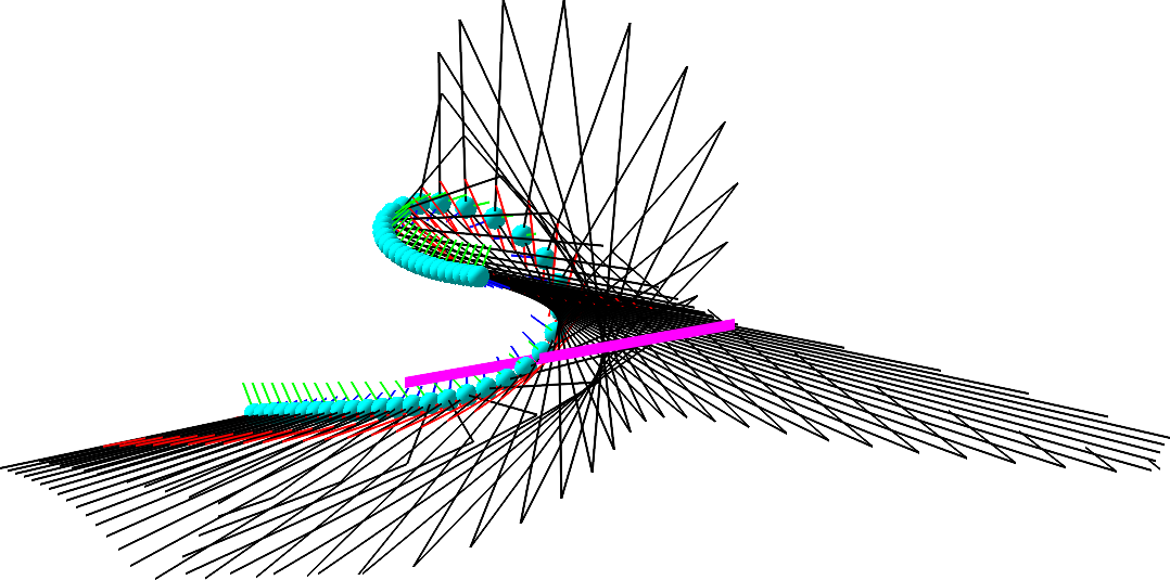
Figure 5. Example 22. The camera center ${{\color[rgb]{0,1,1}C}}$ (cyan) moves along a twisted cubic $\mathcal{C}$. All rolling planes $\Sigma$ (black) intersect in the line ${{\color[rgb]{1,0,1}K}=(0:X_{0}:X_{3}:X_{0})}$ (magenta). $\mathcal{C}$ intersects ${{\color[rgb]{1,0,1}K}}$ in $(0:0:1:0)$ and $(0:1:-1:1)$.

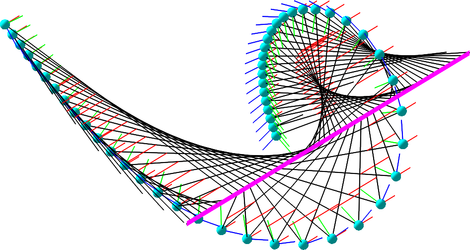
Figure 6. Example 23. The camera center ${{\color[rgb]{0,1,1}C}}$ (cyan) moves along a twisted cubic $\mathcal{C}$. All rolling planes $\Sigma$ (black) intersect in the line ${{\color[rgb]{1,0,1}K}=(0:X_{2}:0:X_{0})}$ (magenta). $\mathcal{C}$ does not intersect ${{\color[rgb]{1,0,1}K}}$.

References

- [1] Marci Meingast, Christopher Geyer, and Shankar Sastry. Geometric models of rolling-shutter cameras. In Omnidirectional Vision, Camera Networks and Non-classical Cameras, 04 2005.
- [2] Omar Ait-aider, Nicolas Andreff, Jean Marc Lavest, and Philippe Martinet. Simultaneous object pose and velocity computation using a single view from a rolling shutter camera. In ECCV, pages 56–68, 2006.
- [3] O. Ait-Aider and F. Berry. Structure and kinematics triangulation with a rolling shutter stereo rig. In ICCV, 2009.
- [4] Guillaume Batog, Xavier Goaoc, and Jean Ponce. Admissible linear map models of linear cameras. In The Twenty-Third IEEE Conference on Computer Vision and Pattern Recognition, CVPR 2010, San Francisco, CA, USA, 13-18 June 2010, pages 1578–1585. IEEE Computer Society, 2010.
- [5] Johan Hedborg, Per-Erik Forssén, Michael Felsberg, and Erik Ringaby. Rolling shutter bundle adjustment. In CVPR, 2012.
- [6] Ludovic Magerand, Adrien Bartoli, Omar Ait-Aider, and Daniel Pizarro. Global optimization of object pose and motion from a single rolling shutter image with automatic 2d-3d matching. In ECCV, 2012.
- [7] Luc Oth, Paul Timothy Furgale, Laurent Kneip, and Roland Siegwart. Rolling Shutter Camera Calibration. In CVPR, 2013.
- [8] Olivier Saurer, Kevin Köser, Jean-Yves Bouguet, and Marc Pollefeys. Rolling Shutter Stereo. In ICCV, 2013.
- [9] Olivier Saurer, Marc Pollefeys, and Gim Hee Lee. A minimal solution to the rolling shutter pose estimation problem. In IROS, 2015.
- [10] Cenek Albl, Zuzana Kukelova, and Tomas Pajdla. R6P - rolling shutter absolute pose problem. In CVPR, 2015.
- [11] Cenek Albl, Zuzana Kukelova, and Tomas Pajdla. Rolling shutter absolute pose problem with known vertical direction. In CVPR, 2016.
- [12] Cenek Albl, Akihiro Sugimoto, and Tomas Pajdla. Degeneracies in rolling shutter sfm. In ECCV, 2016.
- [13] Yuchao Dai, Hongdong Li, and Laurent Kneip. Rolling shutter camera relative pose: Generalized epipolar geometry. In Proceedings of the IEEE Conference on Computer Vision and Pattern Recognition, pages 4132–4140, 2016.
- [14] Eisuke Ito and Takayuki Okatani. Self-Calibration-Based Approach to Critical Motion Sequences of Rolling-Shutter Structure From Motion. In CVPR, 2017.
- [15] Bingbing Zhuang, Loong-Fah Cheong, and Gim Hee Lee. Rolling-Shutter-Aware Differential SfM and Image Rectification. In ICCV, 2017.
- [16] Zuzana Kukelova, Cenek Albl, Akihiro Sugimoto, and Tomas Pajdla. Linear solution to the minimal absolute pose rolling shutter problem. In ACCV, 2018.
- [17] Yizhen Lao and Omar Ait-Aider. A robust method for strong rolling shutter effects correction using lines with automatic feature selection. In CVPR, 2018.
- [18] Pulak Purkait and Christopher Zach. Minimal solvers for monocular rolling shutter compensation under ackermann motion. In WACV, 2018.
- [19] Subeesh Vasu, Mahesh Mohan M. R., and A. N. Rajagopalan. Occlusion-Aware Rolling Shutter Rectification of 3d Scenes. In CVPR, 2018.
- [20] Cenek Albl, Zuzana Kukelova, Viktor Larsson, and Tomas Pajdla. Rolling shutter camera absolute pose. IEEE Trans. Pattern Anal. Mach. Intell., 42(6):1439–1452, 2019.
- [21] Bingbing Zhuang, Quoc-Huy Tran, Pan Ji, Loong-Fah Cheong, and Manmohan Chandraker. Learning structure-and-motion-aware rolling shutter correction. In CVPR, 2019.
- [22] Cenek Albl, Zuzana Kukelova, Viktor Larsson, Michal Polic, Tomas Pajdla, and Konrad Schindler. From two rolling shutters to one global shutter. In Proceedings of the IEEE/CVF Conference on Computer Vision and Pattern Recognition, pages 2505–2513, 2020.
- [23] Bin Fan, Yuchao Dai, and Mingyi He. Rolling shutter camera: Modeling, optimization and learning. Mach. Intell. Res., 20(6):783–798, 2023.
- [24] Praveen K, Lokesh Kumar T, and A. N. Rajagopalan. Deep network for rolling shutter rectification. CoRR, abs/2112.06170, 2021.
- [25] Yizhen Lao, Omar Ait-Aider, and Adrien Bartoli. Solving rolling shutter 3d vision problems using analogies with non-rigidity. Int. J. Comput. Vis., 129(1):100–122, 2021.
- [26] Bin Fan and Yuchao Dai. Inverting a rolling shutter camera: Bring rolling shutter images to high framerate global shutter video. In 2021 IEEE/CVF International Conference on Computer Vision, ICCV 2021, Montreal, QC, Canada, October 10-17, 2021, pages 4208–4217. IEEE, 2021.
- [27] Zhihang Zhong, Yinqiang Zheng, and Imari Sato. Towards rolling shutter correction and deblurring in dynamic scenes. In IEEE Conference on Computer Vision and Pattern Recognition, CVPR 2021, virtual, June 19-25, 2021, pages 9219–9228. Computer Vision Foundation / IEEE, 2021.
- [28] Bin Fan, Yuchao Dai, Zhiyuan Zhang, and Ke Wang. Differential sfm and image correction for a rolling shutter stereo rig. Image Vis. Comput., 124:104492, 2022.
- [29] Fang Bai, Agniva Sengupta, and Adrien Bartoli. Scanline homographies for rolling-shutter plane absolute pose. In IEEE/CVF Conference on Computer Vision and Pattern Recognition, CVPR 2022, New Orleans, LA, USA, June 18-24, 2022, pages 8983–8992. IEEE, 2022.
- [30] Bangyan Liao, Delin Qu, Yifei Xue, Huiqing Zhang, and Yizhen Lao. Revisiting rolling shutter bundle adjustment: Toward accurate and fast solution. In IEEE/CVF Conference on Computer Vision and Pattern Recognition, CVPR 2023, Vancouver, BC, Canada, June 17-24, 2023, pages 4863–4871. IEEE, 2023.
- [31] Bin Fan, Yuchao Dai, and Hongdong Li. Rolling shutter inversion: Bring rolling shutter images to high framerate global shutter video. IEEE Trans. Pattern Anal. Mach. Intell., 45(5):6214–6230, 2023.
- [32] Petr Hruby, Timothy Duff, Anton Leykin, and Tomas Pajdla. Learning to solve hard minimal problems. In IEEE/CVF Conference on Computer Vision and Pattern Recognition, CVPR 2022, New Orleans, LA, USA, June 18-24, 2022, pages 5522–5532. IEEE, 2022.
- [33] Z. Kukelova, M. Bujnak, and T. Pajdla. Automatic Generator of Minimal Problem Solvers. In ECCV, 2008.
- [34] Viktor Larsson, Magnus Oskarsson, Kalle Åström, Alge Wallis, Zuzana Kukelova, and Tomás Pajdla. Beyond grobner bases: Basis selection for minimal solvers. In 2018 IEEE Conference on Computer Vision and Pattern Recognition, CVPR 2018, Salt Lake City, UT, USA, June 18-22, 2018, pages 3945–3954. Computer Vision Foundation / IEEE Computer Society, 2018.
- [35] Evgeniy Martyushev, Jana Vráblíková, and Tomas Pajdla. Optimizing elimination templates by greedy parameter search. In Proceedings of the IEEE/CVF Conference on Computer Vision and Pattern Recognition (CVPR), pages 15754–15764, June 2022.
- [36] Ricardo Fabbri, Timothy Duff, Hongyi Fan, Margaret H. Regan, David da Costa de Pinho, Elias P. Tsigaridas, Charles W. Wampler, Jonathan D. Hauenstein, Peter J. Giblin, Benjamin B. Kimia, Anton Leykin, and Tomas Pajdla. Trifocal relative pose from lines at points. IEEE Trans. Pattern Anal. Mach. Intell., 45(6):7870–7884, 2023.
- [37] Paul Breiding and Sascha Timme. HomotopyContinuation.jl: A package for homotopy continuation in julia, 2018.
- [38] Petr Hruby, Viktor Korotynskiy, Timothy Duff, Luke Oeding, Marc Pollefeys, Tomas Pajdla, and Viktor Larsson. Four-view geometry with unknown radial distortion. In IEEE/CVF Conference on Computer Vision and Pattern Recognition, CVPR 2023, Vancouver, BC, Canada, June 17-24, 2023, pages 8990–9000. IEEE, 2023.
- [39] Richard Hartley and Andrew Zisserman. Multiple view geometry in computer vision. Cambridge university press, 2003.
- [40] Cenek Albl, Zuzana Kukelova, and Tomas Pajdla. R6P – rolling shutter absolute pose problem. In Proceedings of the IEEE Conference on Computer Vision and Pattern Recognition, pages 2292–2300, 2015.
- [41] Jean Ponce, Bernd Sturmfels, and Mathew Trager. Congruences and concurrent lines in multi-view geometry. Advances in Applied Mathematics, 88:62–91, 2017.
- [42] Steven M. Seitz and Jiwon Kim. The space of all stereo images. Int. J. Comput. Vis., 48(1):21–38, 2002.
- [43] Tomas Pajdla. Stereo with oblique cameras. Int. J. Comput. Vis., 47(1-3):161–170, 2002.
- [44] Jean Ponce. What is a camera? In 2009 IEEE Computer Society Conference on Computer Vision and Pattern Recognition (CVPR 2009), 20-25 June 2009, Miami, Florida, USA, pages 1526–1533. IEEE Computer Society, 2009.
- [45] Matthew Trager, Bernd Sturmfels, John F. Canny, Martial Hebert, and Jean Ponce. General models for rational cameras and the case of two-slit projections. CoRR, abs/1612.01160, 2016.
- [46] Richard Hartley and Andrew Zisserman. Multiple View Geometry in Computer Vision. Cambridge, 2nd edition, 2003.
- [47] Jean Ponce, Bernd Sturmfels, and Mathew Trager. Congruences and concurrent lines in multi-view geometry. Advances in Applied Mathematics, 88:62–91, 2017.
- [48] Charles Minshall Jessop. A Treatise on the Line Complex. Cambridge University Press, 1903.
- [49] Timothy Duff, Viktor Korotynskiy, Tomas Pajdla, and Margaret H Regan. Galois/monodromy groups for decomposing minimal problems in 3d reconstruction. SIAM Journal on Applied Algebra and Geometry, 6(4):740–772, 2022.
- [50] Ernst Eduard Kummer. Über die algebraischen Strahlensysteme, in’s Besondere über die der ersten und zweiten Ordnung. Königl. Akademie der Wissenschaften zu Berlin, 1866.
- [51] Pietro De Poi. Congruences of lines with one-dimensional focal locus. Portugaliae Mathematica, 61:329–338, 2004.
- [52] Patrick Le Barz. Formules pour les espaces multisécants aux courbes algébriques. Comptes Rendus Mathematique, 340(10):743–746, 2005.
- [53] Ph Ellia and Davide Franco. Gonality, clifford index and multisecants. Journal of Pure and Applied Algebra, 158(1):25–39, 2001.
- [54] Daniel R. Grayson and Michael E. Stillman. Macaulay2, a software system for research in algebraic geometry. http://www2.macaulay2.com.