Probing multi-particle bunching from intermittency analysis
in relativistic heavy-ion collisions
Abstract
It has been demonstrated that intermittency, a self-similar correlation regarding the size of the phase space volume, exhibits sensitivity to particle bunching within a system situated in the two-dimensional cell. Based on recent findings concerning fluctuations in charge particle density observed in central Au + Au collisions at various energies ranging from = 7.7 to 200 GeV at RHIC/STAR, it is proposed that analyzing intermittency in relativistic heavy-ion collisions could serve as a method to investigate density fluctuations linked to correlation phenomena. Our understanding of particle production mechanisms may be enriched by using intermittency analysis to gain new information contained in them that was previously unavailable.
pacs:
XXXI Introduction
The major goal of the intermittency analysis in relativistic heavy ion collision programs is to explore the phase diagram of quantum chromodynamic (QCD) matter. The critical end point (CEP) is a key feature of the QCD phase diagram, representing the point where the first-order phase transition boundary terminates [1, 2]. Many efforts have been made to search for the possible CEP in heavy-ion collisions [3, 4].
Recently, there has been discussion regarding the potential of particle density fluctuations in heavy-ion collisions to serve as a distinctive indicator of the phase transition within the QCD phase diagram [5, 6]. Critical opalescence, a notable light scattering phenomenon observed in continuous (or second-order) phase transitions in conventional quantum electrodynamic matter [7, 8], is characterized by significant fluctuations within the critical region. In the context of heavy-ion collisions, akin to conventional critical opalescence, it is anticipated that the produced matter would exhibit pronounced particle density fluctuations close to the CEP due to the rapid increase in correlation length within the critical region [9, 10]. Such large density fluctuations are expected to persist through the kinetic freeze-out stage if they can withstand final-state interactions during the hadronic evolution of the system.
Upon approaching a critical point, the correlation length of the system diverges and the system becomes scale invariant, or self-similar [11, 12, 13]. Based on the 3D-Ising universality class arguments [14, 15, 16, 17], the density-density correlation function for small momentum transfer has a power-law structure, leading to large density fluctuations in heavy-ion collisions [14, 15, 16, 17]. Such fluctuations can be probed in transverse momentum phase space within the framework of an intermittency analysis by utilizing the scaled factorial moments [14, 15, 16, 17, 18, 19]. The methodology consists of dividing the D-dimensional phase space into equal-sized cells and the observable, -th order scaled factorial moment , is defined as follows [14, 20, 21, 22, 23, 24]:
| (1) |
where is the number of cells in D-dimensional phase space and is the measured multiplicity of a given event in the -th cell. The angle bracket denotes an average over the events. The intermittency appears as a power-law (scaling) behavior of scaled factorial moments [14, 20, 16, 23]. If the system features density fluctuations, scaled factorial moments will obey a power-law behavior of , , where is called the intermittency index quantifying the strength of intermittency [14, 15, 16, 18, 21].
However, the consideration of ”intermittency” as a genuinely novel phenomenon remained less apparent. Relation between Hanbury-Brown-Twiss effect and intermitency phenomenon was discussed and advocate that they are perfectly compatible [25, 26]. Has been shown that the multi-particle Bose-Einstein correlations leads to the power-law like behavior of scaled factorial moments. In Ref. [27], diverse datasets were analyzed, leading to the conclusion that intermittency results from Bose-Einstein correlations, alongside a mechanism driving power-law behavior. Conversely, in Ref. [28], the authors contend that the observed intermittent-like patterns in moments of multiplicity distributions are attributable to the quantum statistical properties of the particle-emitting system, rather than serving as direct evidence of intermittency.
Notice that implementing the ”mixed event method” effectively removes contributions of multiplicity fluctuations (among others background contributions) [18, 21, 22]. Mixed events are constructed by randomly selecting particles from different original events, while ensuring that the mixed events have the same multiplicity and momentum distributions as the original events. Usually instead of the following observable is used:
| (2) |
where the moments from mixed events are subtracted from the data.
Recently the STAR Collaboration published extensive data on in two dimensional () transverse momentum plane () from central Au+Au collisions at = 7.7, 11.5, 19.6, 27, 39, 62.4 and 200 GeV [29]. In the next sections, based on the STAR experiment data, we provide a discussion concerning multi-particle bunching and suggest that measuring the intermittency in relativistic heavy-ion collisions could serve as a means to investigate density fluctuations within a highly constrained number of cells. This observation will be our main point for further discussion and calculations described in next sections.
II Multiplicity distributions of particles in cells
For large number of cells (where ), the average multiplicity in a cell is small and usually one observes zero or one particle in a given cell. In such a case the multiplicity distributions of particles in a cell are indistinguishable. Considering two borderline multiplicity distributions111For -particle correlation function we have Bose-Einstein distribution, while for Poisson distribution . Between these distributions we have negative binomial distribution and with real positive parameter . The dependence is a consequence of Wick’s theorem [30] and its validity was first demonstrated with thermal photons [31] and recently proved for massive particles [32]., Poisson distribution:
| (3) |
and geometric (Bose-Einstein) distribution:
| (4) |
one can see that for small , and for Poisson distribution, and similarly and for geometric distribution [33].
Assuming that Bose-Einstein correlated bunch of particles appears only in one cell, one have (for large number of cells): and finally
| (5) |
where is the average multiplicity for and
| (6) |
is the factorial moment averaged over multiplicity distribution in a cell with bunch of particles. For geometric distribution (4) with the average multiplicity one have , and from Eq. (5) one can evaluate
| (7) |
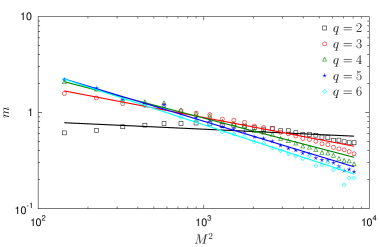
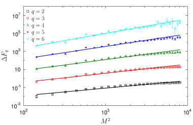
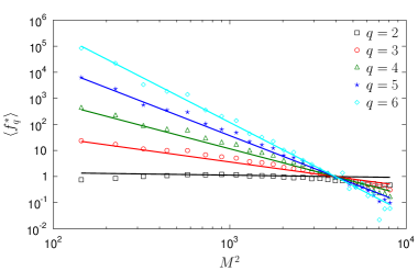
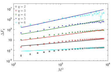
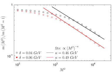
Fig. 1 shows average multiplicity in a bunch evaluated from experimental values. Roughly with and . Fig. 2 shows corresponding values compared to experimental data. Without assumption on multiplicity distribution of particle’s bunch one can evaluate factorial moments (see Fig. 3) and estimate multiplicity distribution in a bunch. From Eq. (6) one can write
| (8) |
and
| (9) |
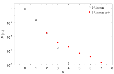
where we put in calculations and . Estimated multiplicity distributions in cells (for taken at and GeV) is presented in Fig. 4. In one cell we have particle bunch with given by Eq. (9) and multiplicity distributions in all the other cells are given by Poisson distribution (3) with .
III Many bunches case
For the case with bunches with multiplicity governed by geometric distribution (4) one have negative binomial distribution (NBD)
| (10) |
and factorial moments
| (11) |
Correlations being a signature of Bose-Einstein statistics never reaches its maximum allowed degree, the most natural interpretation is that the source is not totally chaotic as would be expected from a purely thermalized system, but that a certain degree of coherence () is present in the boson radiation [34]. Effective factorial moments are expected to be
| (12) |
where (c.f. Eq. (11)) and are factorial moments for negative binomial and Poisson distributions, respectively. In this case, one have
| (13) |
Expected in comparison with experimental data are shown in Fig. 5. Comparing Eq. (13) with experimental values at GeV, we estimate roughly and . For small -parameter, Eq. (13) leads to relation and for evaluated -parameter we have dependence
| (14) |
IV Energy dependence
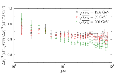
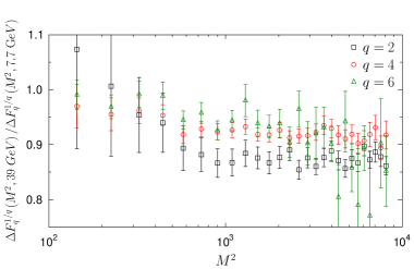
Scaled factorial moments are weekly dependent on collision energy. In Figs. 6 and 7 we show ratios
and , respectively, for different energies and different values of order . Taking into account Eq. (7), this ratio corresponds with ratios at different energies. For large , . Weak energy dependence indicate that energy dependence follows energy dependence of total multiplicity .
V Possible origin of power-law behavior
Intermittency appears as a power-law behavior of scaled factorial moments, . For a scenario in which a bunch of particles appears only in one cell (or in a limiting number of cells), following Eq. (5), we expect the intermittency index , for multiplicity of particles in a bunch being independent on the number of cells . In reality, the division procedure of phase space changes multiplicity in a cell. Number of particles in bunch of effective space size in cell of size is expected to be .
Let’s consider a bunch of particles of transverse size (dispersion with respect to the axis of a bundle) in the random direction with a transverse momentum distribution
| (15) |
Numerical results of the dependence are shown in Fig. 8. For large we observe power-law dependence:
| (16) |
which will result in
| (17) |
The intermittency index is the result of the division procedure, which leads to power-law dependence given by Eq. (16). It is known [35] that, if function follows a simple power law, then it is scale invariant and
| (18) |
with relation . Selecting different functions changes details but the scale invariant behavior is still visible.
VI Conclusions
Density fluctuations in cells lead to the power-law-like behavior of scaled factorial moments. Correlated bunch of particles which appears only in one cell can be responsible for a ”intermittent-like” behavior of . Multiplicity distribution in a bunch of particles and spatial distribution determine behavior of scaled factorial moments. For small size of cell , multiplicity in a bunch with size is scale invariant (its form follows a simple power law ) which will result in . Whether such a simple scenario is related to the broad spectrum of experimental data further calculations from dynamical modeling of heavy-ion collisions are required.
Acknowledgments
This research was supported by the Polish National Science Centre (NCN) Grant 2020/39/O/ST2/00277. In preparation of this work we used the resources of the Center for Computation and Computational Modeling of the Faculty of Exact and Natural Sciences of the Jan Kochanowski University of Kielce.
References
- [1] E. S. Bowman and J. I. Kapusta, Phys. Rev. C 79 (2009), 015202 doi:10.1103/PhysRevC.79.015202 [arXiv:0810.0042 [nucl-th]].
- [2] Y. Hatta and M. A. Stephanov, Phys. Rev. Lett. 91 (2003), 102003 [erratum: Phys. Rev. Lett. 91 (2003), 129901] doi:10.1103/PhysRevLett.91.102003 [arXiv:hep-ph/0302002 [hep-ph]].
- [3] A. Bzdak, S. Esumi, V. Koch, J. Liao, M. Stephanov and N. Xu, Phys. Rept. 853 (2020), 1-87 doi:10.1016/j.physrep.2020.01.005 [arXiv:1906.00936 [nucl-th]].
- [4] X. Luo, Q. Wang, N. Xu, P. Zhuang (Eds.), Properties of QCD Matter at High Baryon Density, Springer, 2022.
- [5] F. Li and C. M. Ko, Phys. Rev. C 93 (2016) no.3, 035205 doi:10.1103/PhysRevC.93.035205 [arXiv:1601.00026 [nucl-th]].
- [6] K. J. Sun, L. W. Chen, C. M. Ko, J. Pu and Z. Xu, Phys. Lett. B 781 (2018), 499-504 doi:10.1016/j.physletb.2018.04.035 [arXiv:1801.09382 [nucl-th]].
- [7] H. Brumberger, N. G. Alexandropoulos and W. Claffey, Phys. Rev. Lett. 19 (1967), 555 doi:10.1103/PhysRevLett.19.555
- [8] A. Lesne, Renormalization Methods; Critical Phenom-ena, Chaos, Fractal Structures (John Wiley and Sons, New York, 1998).
- [9] M. A. Stephanov, K. Rajagopal and E. V. Shuryak, Phys. Rev. Lett. 81 (1998), 4816-4819 doi:10.1103/PhysRevLett.81.4816 [arXiv:hep-ph/9806219 [hep-ph]].
- [10] B. Berdnikov and K. Rajagopal, Phys. Rev. D 61 (2000), 105017 doi:10.1103/PhysRevD.61.105017 [arXiv:hep-ph/9912274 [hep-ph]].
- [11] E. A. De Wolf, I. M. Dremin and W. Kittel, Phys. Rept. 270 (1996), 1-141 doi:10.1016/0370-1573(95)00069-0 [arXiv:hep-ph/9508325 [hep-ph]].
- [12] A. Bialas and R. C. Hwa, Phys. Lett. B 253 (1991), 436-438 doi:10.1016/0370-2693(91)91747-J
- [13] H. Satz, Nucl. Phys. B 326 (1989), 613-618 doi:10.1016/0550-3213(89)90546-4
- [14] N. G. Antoniou, F. K. Diakonos, A. S. Kapoyannis and K. S. Kousouris, Phys. Rev. Lett. 97 (2006), 032002 doi:10.1103/PhysRevLett.97.032002 [arXiv:hep-ph/0602051 [hep-ph]].
- [15] N. G. Antoniou, F. K. Diakonos, X. N. Maintas and C. E. Tsagkarakis, Phys. Rev. D 97 (2018) no.3, 034015 doi:10.1103/PhysRevD.97.034015 [arXiv:1705.09124 [hep-ph]].
- [16] N. G. Antoniou, Y. F. Contoyiannis, F. K. Diakonos, A. I. Karanikas and C. N. Ktorides, Nucl. Phys. A 693 (2001), 799-824 doi:10.1016/S0375-9474(01)00921-6 [arXiv:hep-ph/0012164 [hep-ph]].
- [17] N. G. Antoniou, N. Davis and F. K. Diakonos, Phys. Rev. C 93 (2016) no.1, 014908 doi:10.1103/PhysRevC.93.014908 [arXiv:1510.03120 [hep-ph]].
- [18] T. Anticic et al. [NA49], Phys. Rev. C 81 (2010), 064907 doi:10.1103/PhysRevC.81.064907 [arXiv:0912.4198 [nucl-ex]].
- [19] J. Wu, Y. Lin, Y. Wu and Z. Li, Phys. Lett. B 801 (2020), 135186 doi:10.1016/j.physletb.2019.135186 [arXiv:1901.11193 [nucl-th]].
- [20] R. C. Hwa and M. T. Nazirov, Phys. Rev. Lett. 69 (1992), 741-744 doi:10.1103/PhysRevLett.69.741
- [21] T. Anticic et al. [NA49], Eur. Phys. J. C 75 (2015) no.12, 587 doi:10.1140/epjc/s10052-015-3738-5 [arXiv:1208.5292 [nucl-ex]].
- [22] N. G. Antoniou, Y. F. Contoyiannis, F. K. Diakonos and G. Mavromanolakis, Nucl. Phys. A 761 (2005), 149-161 doi:10.1016/j.nuclphysa.2005.07.003 [arXiv:hep-ph/0505185 [hep-ph]].
- [23] A. Bialas and R. B. Peschanski, Nucl. Phys. B 273 (1986), 703-718 doi:10.1016/0550-3213(86)90386-X
- [24] A. Bialas and R. B. Peschanski, Nucl. Phys. B 308 (1988), 857-867 doi:10.1016/0550-3213(88)90131-9
- [25] A. Bialas, Acta Phys. Polon. B 23 (1992), 561-567 TPJU-9-92.
- [26] T. Wibig, Phys. Rev. D 53 (1996), 3586-3590 doi:10.1103/PhysRevD.53.3586 [arXiv:hep-ph/9508308 [hep-ph]].
- [27] M. Charlet, Phys. Atom. Nucl. 56 (1993), 1497-1514
- [28] P. Carruthers, E. M. Friedlander, C. C. Shih and R. M. Weiner, Phys. Lett. B 222 (1989), 487-492 doi:10.1016/0370-2693(89)90350-X
- [29] M. Abdulhamid et al. [STAR], Phys. Lett. B 845 (2023), 138165 doi:10.1016/j.physletb.2023.138165 [arXiv:2301.11062 [nucl-ex]].
- [30] G. C. Wick, Phys. Rev. 80 (1950), 268 doi:10.1103/PhysRev.80.268
- [31] R. J. Glauber, Phys. Rev. 130, (1963), 2529 doi:10.1103/PhysRev.130.2529
- [32] R. Dall et al., Nature Phys. 9, (2013), 341 doi:10.1038/nphys2632
- [33] J. W. Goodman, Statistical Optics, Wiley Classics Library Edition Published 2000, A Wiley-Interscience Publication (John Wiley and Sons, New York, Chichester, Weinheim, Brisbane, Singapore, Toronto, 2000).
- [34] G. N. Fowler and R. M. Weiner, Phys. Lett. B 70 (1977), 201-203 doi:10.1016/0370-2693(77)90520-2
- [35] D. Sornette, Phys. Rep. 297 (1998) 239