Concatenate, Fine-tuning, Re-training:
A SAM-enabled Framework for Semi-supervised 3D Medical Image Segmentation

Abstract

Segment Anything Model (SAM) fine-tuning has shown remarkable performance in medical image segmentation in a fully supervised manner, but requires precise annotations. To reduce the annotation cost and maintain satisfactory performance, in this work, we leverage the capabilities of SAM for establishing semi-supervised medical image segmentation models. Rethinking the requirements of effectiveness, efficiency, and compatibility, we propose a three-stage framework, i.e., Concatenate, Fine-tuning, and Re-training (CFR). The current fine-tuning approaches mostly involve 2D slice-wise fine-tuning that disregards the contextual information between adjacent slices. Our concatenation strategy mitigates the mismatch between natural and 3D medical images. The concatenated images are then used for fine-tuning SAM, providing robust initialization pseudo-labels. Afterwards, we train a 3D semi-supervised segmentation model while maintaining the same parameter size as the conventional segmenter such as V-Net. Our CFR framework is plug-and-play, and easily compatible with various popular semi-supervised methods. Extensive experiments validate that our CFR achieves significant improvements in both moderate annotation and scarce annotation across four datasets. In particular, CFR framework improves the Dice score of Mean Teacher from 29.68% to 74.40% with only one labeled data of LA dataset. The code is available at https://github.com/ShumengLI/CFR.

I Introduction

Recently, general foundation models for visual segmentation [1, 2, 3, 4] have attracted widespread attention in the field of medical images owing to their excellent segmentation and generalization capabilities. Although these foundational models have made remarkable progress in medical image analysis, it is sometimes challenging to utilize a unified model to segment all medical images due to the inevitable factors, e.g., specific modalities, complex imaging techniques, and variable tissues. To tackle this issue, several recent works have been proposed to either fine-tune or add additional adapters to borrow the ability of foundation model, e.g., MSA [5] and SAMed [6] derived from Segment Anything Model (SAM) [3], to their specific tasks.

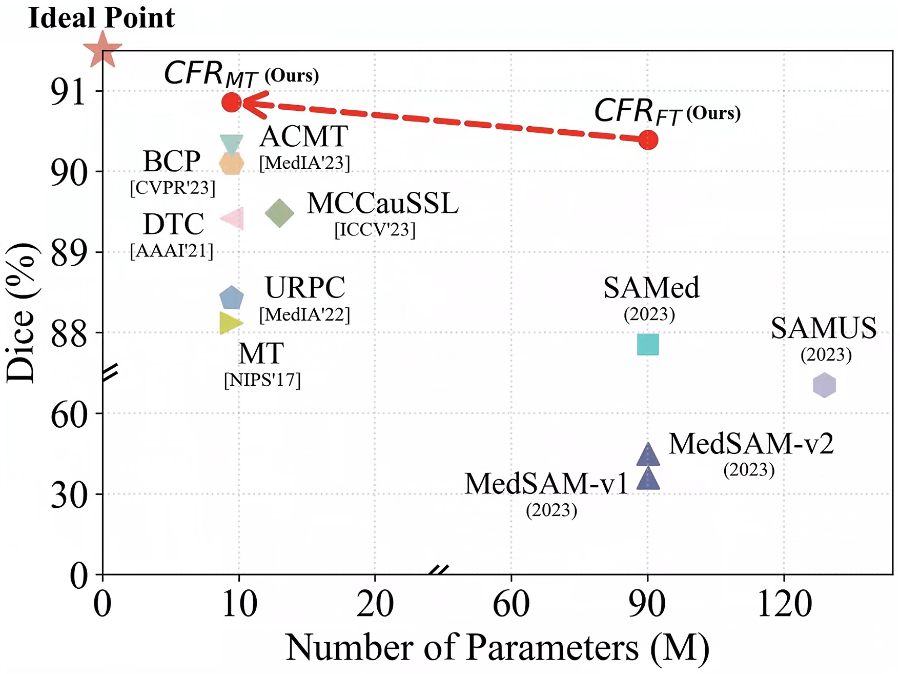
Figure 1: Comparison of our CFR framework with extended foundation models and semi-supervised medical segmentation methods on LA dataset [7] with 16 labeled data.

We notice that all these works are fully supervised methods with fine-tuning or adaptation techniques employed. However, fully supervised medical image segmentation relies on a great amount of precise annotations delineated by experienced experts, which makes the labeling process tedious, time-consuming, and even subjective.

Recent trends [8, 9, 10] have shown that in some cases, the performance of semi-supervised methods is almost comparable to that of fully supervised methods. For example, with 40% annotation, [8] outperforms the fully supervised approach on BTCV dataset. And the performance of [9] on LA dataset with 20% labeled data is only 0.8% lower than the fully supervised result. Therefore, we wonder, whether the current success of the foundation model could drive us to develop an effective and efficient model for semi-supervised medical image segmentation?

With the aforementioned goal, we wish to revisit several important factors before designing our framework for semi-supervised medical image segmentation.

How to initialize effectively? According to previous studies  [11, 12, 13, 14, 15, 10, 16, 9, 8, 17, 18], in the semi-supervised scenario, the quality of pseudo-labels in initialization stages plays an important role in the following segmentation. Unlike natural images, inter-slice continuity of 3D medical images is crucial for accurate target segmentation. Also, medical images usually have relatively low resolution. The existing strategy of fitting medical images, either directly enlarging 2D slices [19] or resizing the positional embeddings [6, 20], disregards the inherent inter-slice correlation that exists in 3D images. Therefore, is there a better way to boost the quality of initial pseudo-labels for medical images using a foundation model?

How to improve efficiency? Foundation model is pre-trained on a large-scale dataset whose parameter size is relatively large. Previous fine-tuning methods [19, 5] still preserve the original parameter size as foundation model during inference. During segmenting medical images, do we really need such a large parameter size? Firstly, the existing model only involving a small-size parameter indeed performs well in segmenting organs [10, 17]. Secondly, we notice that very recent works [21, 22, 23] depict the redundancy issue in the foundation model, revealing that the large-scale pre-trained models are over-parameterized. Thirdly, the appearance of medical images often has standardized views and relatively limited texture variants compared with the natural image [24]. Regarding these aforementioned issues, is it possible to escape from over-parameterized foundation model while maintaining promising results?

How to preserve compatibility? On one hand, in recent years, semi-supervised learning has emerged as an appealing strategy and been widely applied to medical image segmentation tasks [25], and a lot of semi-supervised medical image segmentation methods have been proposed. Could the foundation models be made to better serve existing semi-supervised methods? On the other hand, the research progress in the field of computer vision and machine learning about semi-supervised learning still helps evolve new semi-supervised medical image segmentation models. Will our framework still be compatible with these new methods in the future?

Being aware of these observations, we believe, that in the era of foundation model, a promising semi-supervised medical image segmentation framework should be performance effectiveness, parameter efficiency, and excellent compatableness. Thus, in this paper, we propose a straightforward framework of Concatenate, Fine-tuning, and Re-training (CFR) to accomplish our above goals. We first develop a concatenate strategy, performing a concatenation operation on slices to produce an image that matches the high-resolution input, which better exploits inter-slice relationships and dimensional information. The concatenated images are then fed into the SAM’s image encoder for fine-tuning. Afterwards, we train a small-scale 3D segmentation model with the guidance of SAM while maintaining the same parameter size. The fine-tuned SAM provides a favorable initialization and is able to be compatible with various 3D segmentation models. We conduct the semi-supervised scenarios of moderate annotation and scarce annotation on four datasets. The experiments demonstrate our CFR framework achieves extremely close performance to full supervision with moderate annotation and exhibits remarkable improvement with scarce annotation.

Our contribution could be summarized as follows:

• We propose a novel framework leveraging the ability of the foundation model while ensuring performance under semi-supervised segmentation and further reducing labeling costs, which involves three stages, i.e., concatenate, fine-tuning, and re-training.

• Our concatenate strategy is simple yet effective in pseudo-labeling initialization, and largely distinct from current resize/directly fine-tuning strategy.

• Our parameter size maintains the same level as the mainstream segmenter, e.g., V-Net [26], which is greatly smaller than that of foundation model.

• Our framework is plug-and-play, which could be easily married to most existing popular semi-supervised segmentation methods.

The remaining of this paper is organized as follows: Section II describes the related works on foundation models in medical images and recent semi-supervised techniques. Section III presents our proposed framework, and Sections IV, V, and VI elaborate three modules in detail. Section VII provides a summary of the framework. Section VIII reports and analyzes the experimental results, and Section IX draws the conclusion.

II Related Work

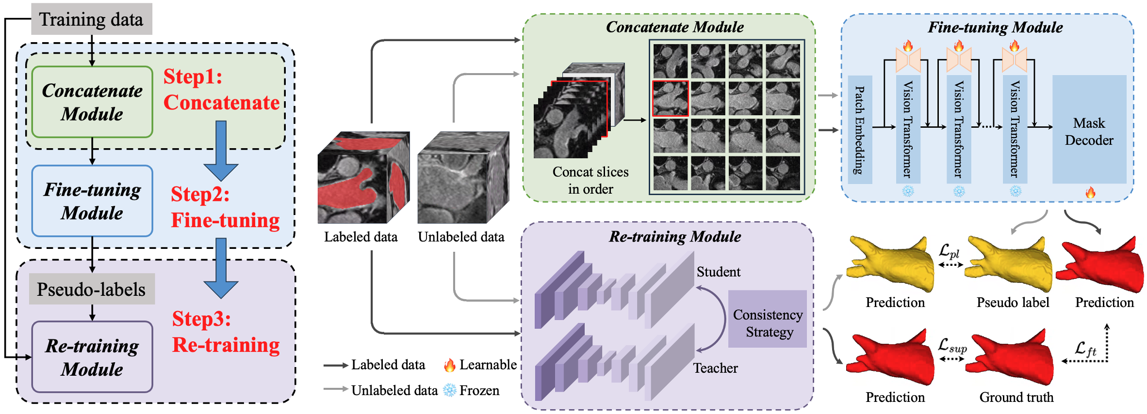
Figure 2: Overview of the proposed CFR framework, which includes three modules: Concatenate, Fine-tuning and Re-training.

II-A Foundation Models in Medical Images

II-A1 Vision Foundation Models

Nowadays, visual foundation models have gained significant attention and have shown impressive performance in various computer vision tasks including segmentation. Prominent examples of these models include SAM [3], SegGPT [1], SEEM [2], and SLiMe [4], along with their extended applications [27, 28, 29]. These models leverage large-scale image datasets to learn universal visual representations and demonstrate remarkable generalization ability.

In the field of medical images, UniverSeg [30] achieves universal segmentation for 2D medical images by providing an example set of image-label pairs. STU-Net [31] is a foundation model specializing in CT modalities, with its largest variant consisting of 1.4 billion parameters. Furthermore, SAM [3] has emerged as one of the most prevailing models for image segmentation, and many works extend it to medical images. SAM-Med2D [32] is a 2D model that fine-tunes SAM on 4.6 million medical images. SAM-Med3D [33] adopts a SAM-like architecture, but it is trained from scratch without utilizing the pre-trained weights of SAM.

Due to SAM’s impressive performance and broad applicability, it serves as the default foundation model in our proposed framework. SAM consists of three components: image encoder, prompt encoder, and mask decoder. The image encoder and prompt encoder extract image features and embed prompts respectively, and the mask decoder receives both embeddings and predicts the masks.

II-A2 Adapt SAM to 3D Medical Images

Due to the lack of medical image data and corresponding semantic labels, SAM’s zero-shot segmentation capability is insufficient to ensure direct application in medical images [34, 35]. To extend the powerful segmentation ability to medical images, many works are devoted to fine-tuning SAM with different image processing and fine-tuning strategies.

For image processing, the disparity in image resolution between 3D medical images and pre-trained natural images poses a challenge, and two strategies have been proposed to tackle this issue. The first is upsampling fine-tuning [19], which involves upsampling each slice to match the input resolution directly. The second is small-size fine-tuning [6, 20], which reduces the input size through bilinear interpolation. However, both of these strategies are based on 2D inputs, and for 3D medical images, the predictions need to be generated by segmenting each slice. [36] and [33] extended SAM to 3D architecture, but it increases additional training overhead with a large model size. Our concatenate strategy takes into account both image dimension and image resolution differences. By creating a large-sized concatenated image, spatial information of adjacent slices could also be captured.

The fine-tuning approaches include fine-tuning only sub-parts parameters and incorporating adapters. [19] froze the image encoder and prompt encoder and only fine-tuned the mask decoder of SAM, but the performance still lags behind medical-specific models, particularly in terms of boundary consensus. [5] and [6] adopted the parameter-efficient fine-tuning techniques, with adapter strategy and low-rank-based fine-tuning strategy (LoRA) [37] respectively for fine-tuning.

II-B Semi-supervised Medical Image Segmentation

Since the pixel-wise annotations require tremendous delineation time, semi-supervised learning (SSL) for segmentation aims to reduce the annotation burden by leveraging a large number of unlabeled samples along with a limited number of labeled samples [12, 13, 14, 15, 10, 16, 9, 8, 17, 18]. Semi-supervised segmentation methods mainly include pseudo-labeling and consistency regularization. Self-training [38, 39, 40] gradually generates pseudo-labels for unlabeled data through an iterative process to be jointly trained with labeled data. Mean Teacher [13] is a classic consistency regularization-based method that effectively reduces over-adaptation. Xu et al . [9] improved the classical MT model to an ambiguity-consensus mean teacher model, and Chen et al . [8] proposed a data augmentation strategy based on partition-and-recovery $N^{3}$ cubes. Existing SSL methods have demonstrated promising results with moderate annotation levels. On one hand, our framework ensures seamless integration with various SSL models. On the other hand, we also apply the framework to challenging scenarios, further reducing the annotation requirements.

Remark. Our framework explores the potential of leveraging SAM’s capabilities in SSL medical image segmentation models, improving accuracy while reducing annotation costs. It is worth mentioning that our framework is compatible with most SSL methods for medical images.

III Framework: CFR

III-A Notations

Formally, we now provide our notation used in this paper. Given $m$ labeled images and $n$ unlabeled images, the $i$-th ($1\leq i\leq m$) labeled image and its ground truth are denoted as $\mathbf{X}^{l}_{i}$ and $\mathbf{Y}^{l}_{i}$. The $j$-th ($1\leq j\leq n$) unlabeled image is denoted as $\mathbf{X}^{u}_{j}$. Here, $\mathbf{X}^{l}_{i}$, $\mathbf{X}^{u}_{j}\in\mathbb{R}^{H\times W\times D}$, $\mathbf{Y}^{l}_{i}\in\{0,1,...,K-1\}^{H\times W\times D}$, where $H$, $W$, $D$ indicate the corresponding dimensionality of 3D medical images and the input patch size for training is square, i.e., $H=W$. $K$ is the number of different classes to segment. Our CFR framework consists of three modules as follows.

III-B Modules

$\blacktriangleright$ Step 1: Concatenate Module. As aforementioned, by reducing the resolution difference between pre-trained samples (i.e., natural image) and fine-tuned samples (i.e., medical image), the concatenate module could transform a 3D labeled volume $\mathbf{X}^{l}_{i}$ to a large-sized 2D image $\mathbf{M}^{l}_{i}\in\mathbb{R}^{Hd\times Wd}$ with a slice concatenation function $\texttt{F}_{\texttt{C}}(\cdot)$. Also, the concatenated ground truth $\mathbf{N}^{l}_{i}$ is obtained similarly. $\mathbf{M}^{l}_{i}$ and $\mathbf{N}^{l}_{i}$ are arranged in an $d\times d$ grid with $d=\lceil\sqrt{D}\rceil$, and we concatenate zeros after all slices if $d\times d>D$.

$$\mathbf{M}^{l}_{i}=\texttt{F}_{\texttt{C}}(\mathbf{X}^{l}_{i}),\qquad\mathbf{N}^{l}_{i}=\texttt{F}_{\texttt{C}}(\mathbf{Y}^{l}_{i}).$$ (1)

$\blacktriangleright$ Step 2: Fine-tuning Module. In this module, we first utilize the concatenated labeled images $\mathbf{M}^{l}_{i}$ along with their ground truth $\mathbf{N}^{l}_{i}$ to fine-tune a SAM parameterized by $\theta$ via popularly used strategy, e.g., LoRA [37, 6]. This aims to narrow the possible distribution shift between natural and medical images. Taking LoRA as an example, we denote the fine-tune function as $\texttt{F}_{\texttt{LoRA}}(\cdot)$, which is parameterized by $\theta$ with input as $\mathbf{M}^{l}_{i}$ and $\mathbf{N}^{l}_{i}$. The updated SAM with optimal parameter $\theta^{*}$ is obtained as follows:

$$\theta^{*}=\arg\min_{\theta}\sum_{i=1}^{m}\texttt{F}_{\texttt{LoRA}}(\mathbf{M}^{l}_{i},\mathbf{N}^{l}_{i};\theta).$$ (2)

Then, we produce high-quality pseudo-labels for unlabeled images by using the prediction function $\texttt{F}_{\texttt{FT}}(\cdot)$ of fine-tuned SAM, and generate 3D pseudo-labels by a concatenated inverse transform $\texttt{F}_{\texttt{C}}^{\texttt{-1}}(\cdot)$ as follows:

$$\hat{\mathbf{Y}}^{u}_{j}=\texttt{F}_{\texttt{C}}^{\texttt{-1}}\Bigl{(}\texttt{F}_{\texttt{FT}}\bigl{(}\texttt{F}_{\texttt{C}}(\mathbf{X}^{u}_{j});\theta^{*}\bigr{)}\Bigr{)}.$$ (3)

$\blacktriangleright$ Step 3: Re-training SSL Module. The recent SSL network, such as the popular self-training, mean teacher, and the most advanced ACMT, MagicNet methods, could be the alternatives in this module. Specifically, the SSL network learns pseudo-labels from fine-tuned SAM. We denote the SSL network as $\texttt{F}_{\texttt{S}}(\cdot)$ parameterized by $\omega$ and the re-training module with optimal $\omega^{*}$ is as follows:

$$\omega^{*}=\arg\min_{\omega}\bigl{(}\sum_{i=1}^{m}\texttt{F}_{\texttt{S}}(\mathbf{X}^{l}_{i},\mathbf{Y}^{l}_{i};\omega)+\lambda\sum_{j=1}^{n}\texttt{F}_{\texttt{S}}(\mathbf{X}^{u}_{j},\hat{\mathbf{Y}}^{u}_{j};\omega)\bigr{)},$$ (4)

where $\lambda$ acts as a tradeoff between two terms.

IV Concatenate Module

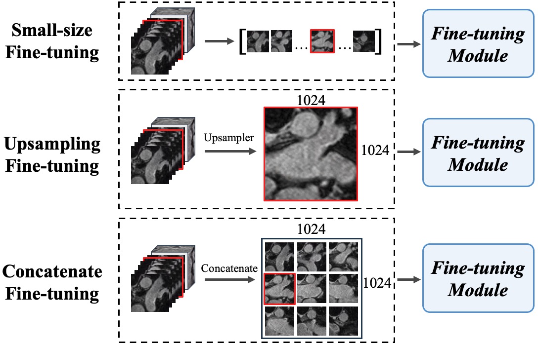
Figure 3: Fine-tuning input strategies comparison. Small-size fine-tuning reduces the input size through bilinear interpolation and upsampling fine-tuning directly upsamples each slice. Taking $d=3$ as an example.

To adapt from 2D natural images to 3D medical images, we recognize that the input resolution and image dimension are crucial factors. The inter-slice spatial information of 3D volumes is relevant for target recognition, and it is difficult for the large model trained at high-resolution images to generalize to low-resolution medical image slices.

Inspired by this, our concatenate strategy, illustrated in Figure 3, matches medical images to natural image resolution, and supplements the spatial arrangement specific to 3D medical images. The input spatial resolution of the pre-trained SAM model is $1024\times 1024$. Our concatenate strategy flattens the 3D volume (3D raw image or 3D patch) slice by slice and arranges them in an $d\times d$ grid, forming a 2D image with size $1024\times 1024$. Considering that the slice sizes of original medical 3D datasets might vary a lot in different cases, how to concatenate should be analyzed case by case. For the small-scale slices, such as the LA and BraTS datasets, we use a raw 3D image as an input volume. For large-scale slices, such as the BTCV and MACT datasets, we follow the common 3D processing way where dividing the volume into patches as an input volume, and then concatenate all slices to achieve the final size of $1024\times 1024$, avoiding downsizing a large slice directly. Compared to the small-size input fine-tuning method [19] and the direct upsampling fine-tuning methods [6, 20] in Figure 5a, we find our concatenate strategy effectively addresses the challenges of image dimension and resolution differences. We thoroughly investigate the concatenate strategy and conduct some empirical analysis.

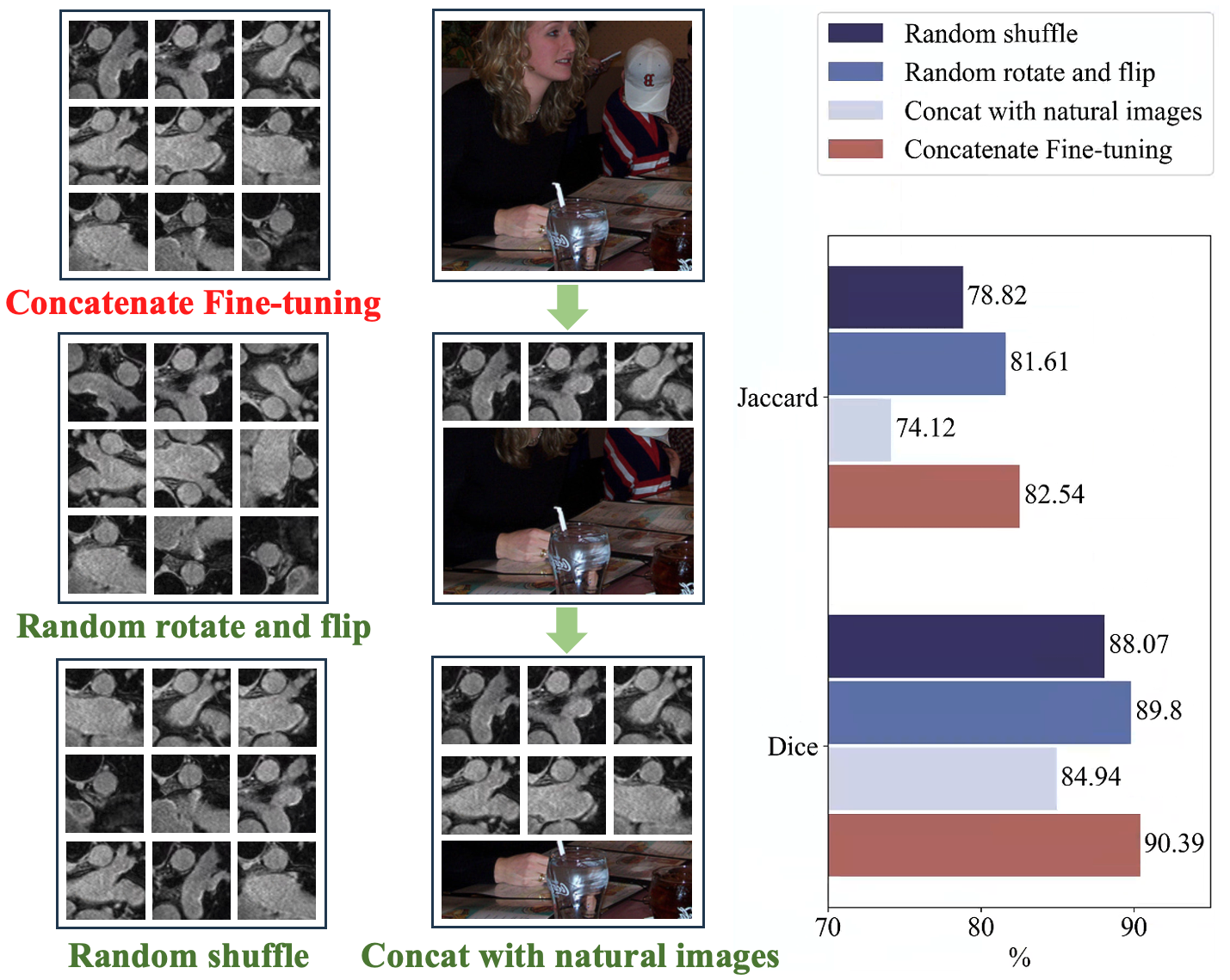
Figure 4: Disrupting slice continuity and contextual integrity. Comparison with random shuffling, random slice rotation and flipping, and concatenation with natural images. $d=3$ as an example.

IV-A Slice Continuity

Due to the inherent spatial continuity of 3D medical images, we explore the relationship between slice concatenation and slice order. For a concatenated 2D image, the segmentation model learns the feature correlation across slices through the self-attention mechanism, so it struggles to capture contextual information and coherence of shape without the slice order. To investigate the importance of slice continuity, we disrupt the continuity in two ways: 1) Randomly shuffling the order of the slices; 2) Randomly rotate and flip each individual slice. As illustrated in Figure 4, it has been observed that disrupting the slice order leads to the loss of shape coherence and a decrease in performance, and the results emphasize the importance of slice continuity in 3D organ segmentation.

IV-B Contextual Integrity

Our concatenate module reorganizes a 3D volume (3D raw image or 3D patch) into a $1024\times 1024$ 2D image, enabling a complete representation of the volume within a single image. To explore the impact of contextual integrity on concatenate fine-tuning, we approach it from two perspectives.

Firstly, we adjust the concatenation scale $d\times d$ as shown in Figure 5b. Take the LA dataset as an example, when the concatenation scale is $9\times 9$, the large-sized 2D image is composed of a complete 3D volume. The results indicate that there is an upward trend in overall performance as the concatenation scale increases. Specifically, the segmentation performance is best when the concatenated image contains the complete 3D volume.

Secondly, while keeping the resolution of each slice constant, we explore the impact of changing the number of slices and concatenating with natural images. As shown in Figure 4, we transition from natural images to medical images by progressively increasing the number of medical slices. The natural images are from the PASCAL VOC 2012 dataset [41]. Although this approach seems to gradually adjust from natural image features to medical image features, it actually disrupts the integrity of the anatomical structure in medical images and leads to a decrease in performance.

These observation results reveal the importance of maintaining slice continuity and contextual integrity for our concatenate strategy, effectively bridging the domain and spatial dimensional gaps between natural and medical images.

(a) Different image resolutions.

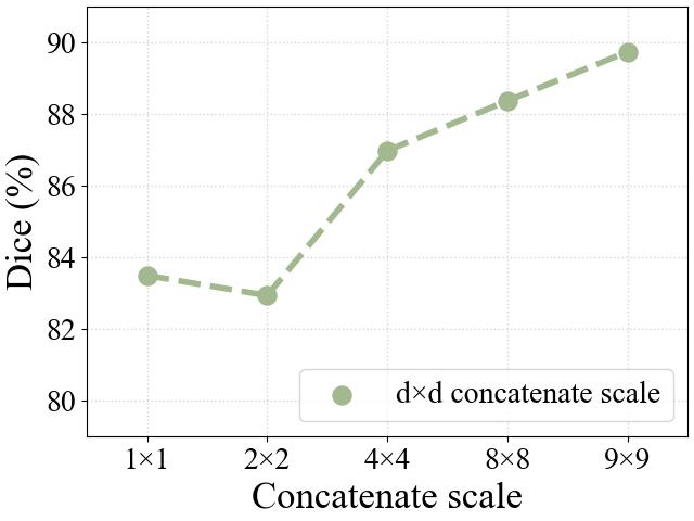
(b) Different concatenate scales.

Figure 5: Fine-tuning with different strategies on LA dataset with 16 labeled data. (a) Comparison with small-size and upsampling fine-tuning. (b) Comparison with different concatenation scales.

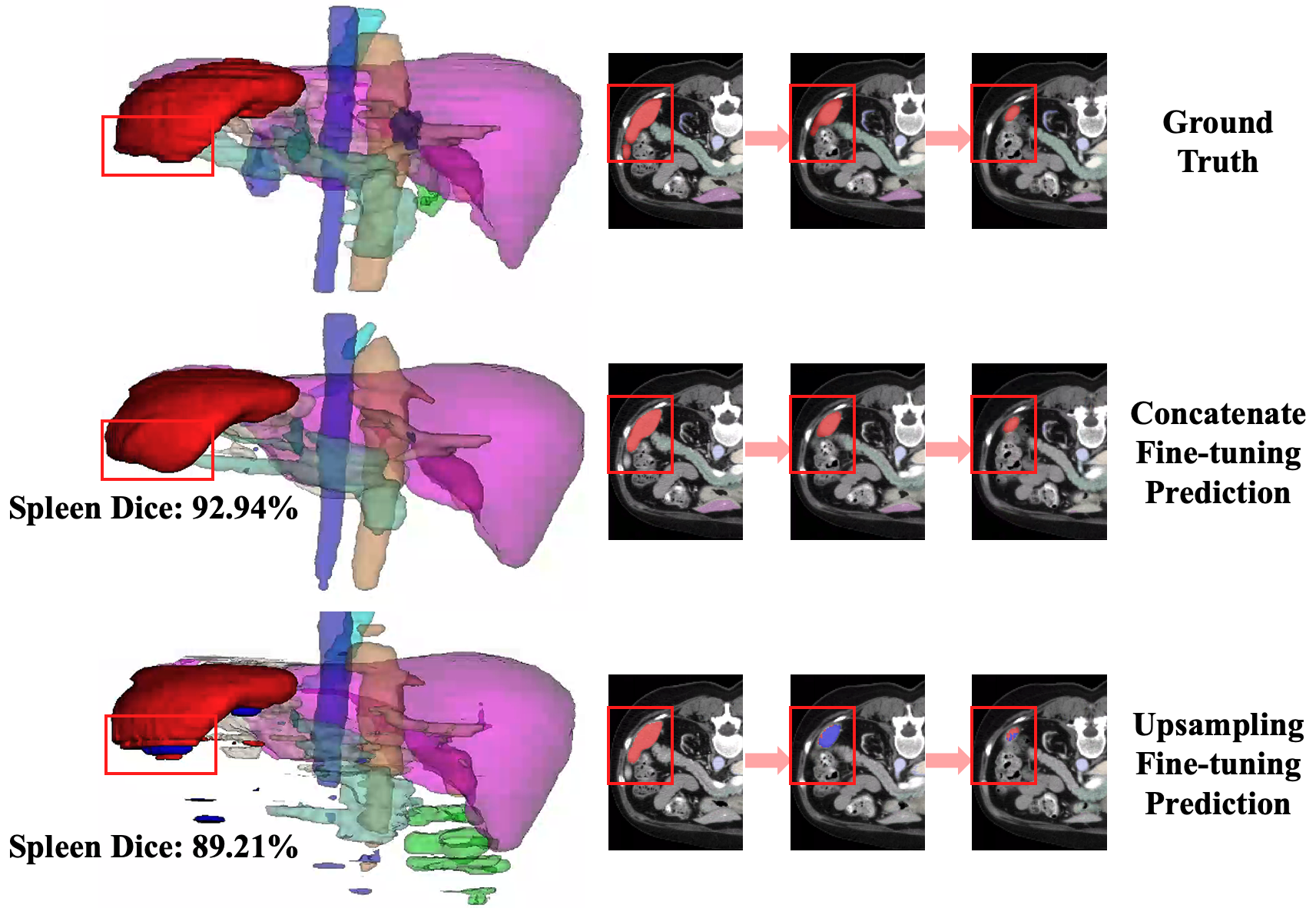
Figure 6: Fine-tuning input strategies comparison. Upsampling fine-tuning directly upsamples each slice.

V Fine-tuning Module

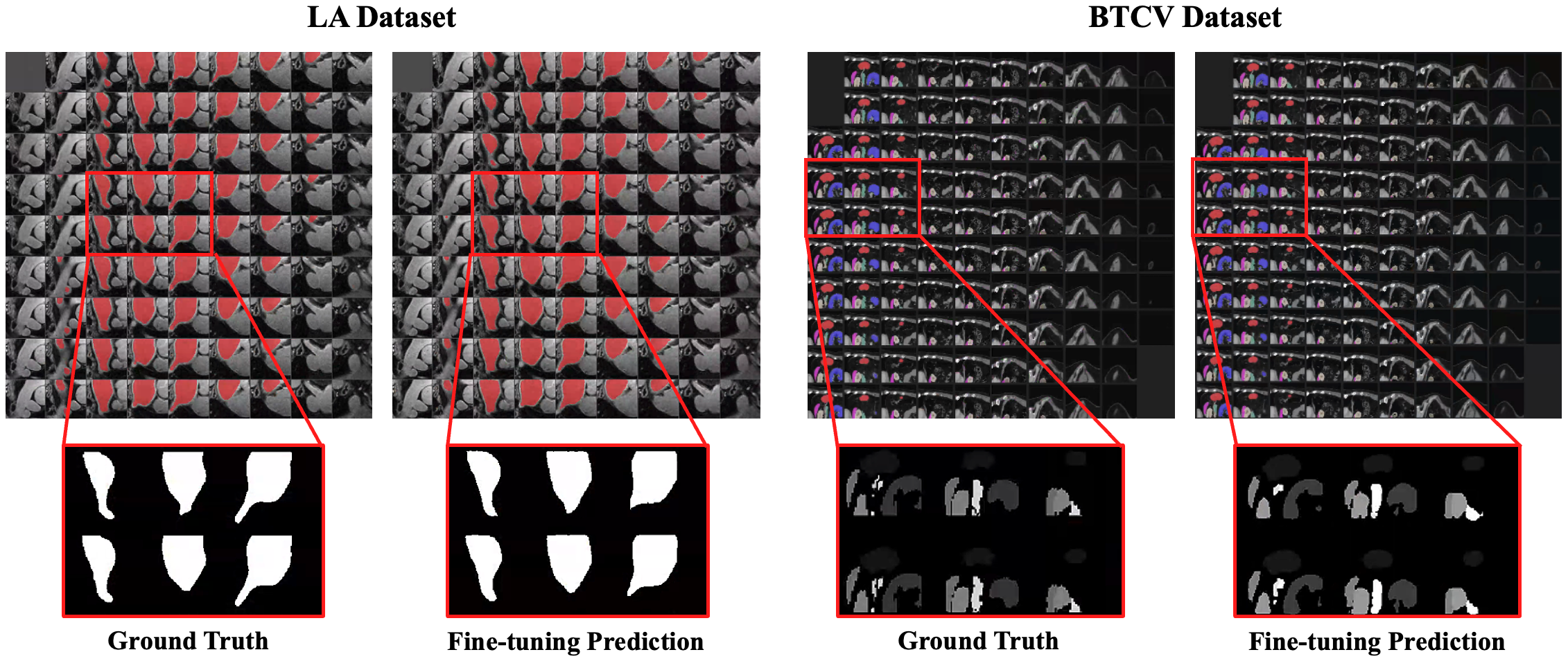
Figure 7: Visualization of fine-tuning module on LA and BTCV dataset.

Our fine-tuning module performs fine-tuning on the vision foundation model. As one of the most popular universal image segmentation models, SAM serves as the default setting of fine-tuning module in our CFR, denoted as $\texttt{F}_{\texttt{FT}}(\cdot)$. We strip away all the task prompts, and perform automatic segmentation during inference. Our framework is not limited to a specific fine-tuning strategy, which could be used in different strategies. We uniformly denote the fine-tuning loss $\mathcal{L}_{ft}$:

$$\mathcal{L}_{ft}=\frac{1}{2}\bigl{(}\mathcal{L}_{Dice}(\mathbf{P}^{l}_{i},\mathbf{N}^{l}_{i})+\mathcal{L}_{ce}(\mathbf{P}^{l}_{i},\mathbf{N}^{l}_{i})\bigr{)},$$ (5)

where $\mathbf{P}^{l}_{i}=\texttt{F}_{\texttt{FT}}(\mathbf{M}^{l}_{i})$ is the prediction of fine-tuning module.

The previous studies mainly involve fine-tuning only sub-parts parameters [19] and incorporating adapters [5, 6].

Sub-parts Fine-tuning. Sub-parts fine-tuning methods directly modify the model parameters. MedSAM-v1 [19] freezes the image encoder and prompt encoder by only fine-tuning the mask decoder, and MedSAM-v2 fine-tunes both image encoder and mask decoder. However, the overall performance still lags behind expert models for medical image segmentation, particularly in terms of boundary consensus.

Adapter Tuning. Adapter tuning [42, 5] is to insert adapters into the original fundamental model, and only tune adapters while leaving all pre-trained parameters frozen. An adapter consists of a down-projection, ReLU activation, and up-projection layers. The low-rank-based fine-tuning strategy (LoRA) [37] injects trainable low-rank decomposition matrices into the layers of the pre-trained model. SAMed [6] freeze the image encoder of SAM, adopt LoRA by adding a bypass, and fine-tune the mask decoder.

Since LoRA can be merged with the original pre-trained weights for inference, we adopt it as our fine-tuning module method $\texttt{F}_{\texttt{LoRA}}(\cdot)$. Following [6], for the classification head of SAM, ambiguity prediction is replaced by the determined prediction output for each semantic category.

We notice that concatenating 2D slices may result in organs appearing in fixed regions, guiding SAM to capture these similarities. As shown in Figure 6, taking the spleen as an example, since the upsampling fine-tuning method predicts slice by slice, it confuses the spleen (red) into the left kidney (blue) between adjacent slices, even when the target is located in the same region across different slices. In contrast, our concatenate strategy preserves the spatial relationship between slices and could leverage the information of the same target from neighboring slices. To verify the effectiveness of pseudo-labels on different datasets, we visualize the fine-tuning module prediction in Figure 7. The mask decoder outputs a large-sized 2D mask, which is subsequently restored to a 3D volume as a pseudo-label for the SSL module.

VI Re-training SSL Module

Input: Labeled images $\{(\mathbf{X}^{l}_{i},\mathbf{Y}^{l}_{i})|1\leq i\leq m\}$, unlabeled images $\{\mathbf{X}^{u}_{j}|1\leq j\leq n\}$, concatenate module $\texttt{F}_{\texttt{C}}$, fine-tuning epochs $T^{\prime}$, total training epochs $T$ and unsupervised loss weight $\lambda$

Output: Trained fine-tuning and re-training modules $\texttt{F}_{\texttt{FT}}$, and $\texttt{F}_{\texttt{S}}$, respectively.

1 Initialize the modules $\texttt{F}_{\texttt{FT}}$, and $\texttt{F}_{\texttt{S}}$

2 for $t\leftarrow 1$ to $T^{\prime}$ do

       // Concatenating

3       $\mathbf{M}^{l}_{i}\leftarrow\texttt{F}_{\texttt{C}}(\mathbf{X}^{l}_{i})$, $\mathbf{N}^{l}_{i}\leftarrow\texttt{F}_{\texttt{C}}(\mathbf{Y}^{l}_{i})$

       // Fine-tuning

4       $\mathcal{L}_{ft}\leftarrow$ using Eq. (5)

5      

6 end for

7Update $\texttt{F}_{\texttt{FT}}$ by minimizing $\mathcal{L}_{ft}$

// SSL re-training

8 for $t\leftarrow T^{\prime}$ to $T$ do

9       foreach $(\mathbf{X}^{l}_{i},\mathbf{Y}^{l}_{i})$ in minibatch do

10             $\mathcal{L}_{sup}\leftarrow\mathcal{L}_{sup}\bigl{(}\texttt{F}_{\texttt{S}}(\mathbf{X}^{l}_{i}),\mathbf{Y}^{l}_{i}\bigr{)}$

11            

12       end foreach

13      foreach $\mathbf{X}^{u}_{j}$ in minibatch do

             // Pseudo label generating

14             pseudo label $\hat{\mathbf{Y}}^{u}_{j}\leftarrow\texttt{F}_{\texttt{C}}^{\texttt{-1}}\Bigl{(}\texttt{F}_{\texttt{FT}}\bigl{(}\texttt{F}_{\texttt{C}}(\mathbf{X}^{u}_{j})\bigr{)}\Bigr{)}$

15             $\mathcal{L}_{pl}\leftarrow$ using Eq. (7)

16             $\mathcal{L}_{unsup}\leftarrow\mathcal{L}_{uns\cdot rt}+\mathcal{L}_{pl}$

17            

18       end foreach

19      $\mathcal{L}_{ssl}\leftarrow\mathcal{L}_{sup}+\lambda\mathcal{L}_{unsup}$

20      

21 end for

22Update $\texttt{F}_{\texttt{S}}$ by minimizing $\mathcal{L}_{ssl}$

Algorithm 1 Training procedure of CFR framework

As defined above, the training data consists of labeled dataset $L=\left\{(X^{l}_{i},Y_{i})\right\}^{m}_{i=1}$ and unlabeled dataset $U=\left\{X^{u}_{j}\right\}^{n}_{j=1}$. The training objective of re-training SSL module $\texttt{F}_{\texttt{S}}(\cdot)$ can be formulated as:

$$\omega^{*}=\arg\min_{\omega}(\mathcal{L}_{sup}+\lambda\mathcal{L}_{unsup}),$$ (6)

where $\mathcal{L}_{sup}$ and $\mathcal{L}_{unsup}$ are supervised and unsupervised terms, respectively, and $\lambda$ acts as a tradeoff between them. Our pseudo-label guidance $\mathcal{L}_{pl}$ is an unsupervised loss.

$$\mathcal{L}_{pl}=\frac{1}{2}\bigl{(}\mathcal{L}_{Dice}(\mathbf{P}^{u}_{j},\hat{\mathbf{Y}}^{u}_{j})+\mathcal{L}_{ce}(\mathbf{P}^{u}_{j},\hat{\mathbf{Y}}^{u}_{j})\bigr{)},$$ (7)

where $\mathbf{P}^{u}_{j}=\texttt{F}_{\texttt{S}}(\mathbf{X}^{u}_{j})$ is the prediction of SSL module.

We investigate four 3D medical image semi-supervised methods for our re-training module, including two classical methods (i.e., self-training and mean teacher), and two advanced methods (i.e., ACMT and MagicNet).

Self-training: Self-training [39] involves three iteratively steps: Firstly, a teacher network is initially trained on $L$. Secondly, it makes predictions on $U$ to obtain $\hat{U}$. Thirdly, a student network retrained on the union set $L\cup\hat{U}$. Among them, steps 2 and 3 are iteratively performed in alternation. The unsupervised loss can be formulated as:

$$\mathcal{L}_{uns\cdot rt}=\mathcal{L}\bigl{(}\texttt{F}_{\texttt{S}}(\mathbf{X}^{u}_{j};\omega^{t}_{\ast}),\texttt{F}_{\texttt{S}}(\mathbf{X}^{u}_{j};\omega^{s})\bigr{)},$$ (8)

where $\omega^{t}$ and $\omega^{s}$ denote the weights of student and teacher networks, and $\ast$ means parameters are fixed.

Mean Teacher: Mean teacher (MT) [13] consists of a student network and a teacher network, and teacher network weights are updated with the exponential moving average (EMA) of student network weights. The unsupervised loss is the consistency regularization between the two networks:

$$\mathcal{L}_{uns\cdot rt}=\mathcal{L}\bigl{(}\texttt{F}_{\texttt{S}}(\mathbf{X};\omega^{t},\xi^{t}),\texttt{F}_{\texttt{S}}(\mathbf{X};\omega^{s},\xi^{s})\bigr{)},$$ (9)

where $\mathbf{X}$ can be a labeled sample $\mathbf{X}^{l}_{i}$ or an unlabeled sample $\mathbf{X}^{u}_{j}$. $\xi^{t}$ and $\xi^{s}$ denote the input data with different perturbations of student and teacher networks respectively.

ACMT: ACMT [9] improves MT to the ambiguity-consensus mean teacher model, encouraging consistency between the student’s and the teacher’s predictions at the identified ambiguous regions. The unsupervised consistency loss is redesigned as ambiguity-masked error:

$$\mathcal{L}_{uns\cdot rt}=\frac{\textstyle\sum_{v}E_{v}\mathcal{L}(\mathbf{P}^{t}_{v},\mathbf{P}^{s}_{v})}{\textstyle\sum_{v}E_{v}},$$ (10)

where $E_{v}$ is the binary ambiguity indicator, and $\mathbf{P}^{t}_{v}$ and $\mathbf{P}^{s}_{v}$ are the predictions of two networks at the $v$-th voxel.

MagicNet: MagicNet [8] introduces a data augmentation strategy based on MT. First, a pair of labeled and unlabeled samples are mixed into two shuffled cubes. Next, small cubes and mixed cubes are fed into the segmentation network, and finally recovery the mixed cubes. The unsupervised loss function consists of two parts:

$$\mathcal{L}_{uns\cdot rt}=\mathcal{L}_{cls}+\mathcal{L}_{blend},$$ (11)

where $\mathcal{L}_{cls}$ is the small cubes location reasoning loss, and $\mathcal{L}_{blend}$ is the mix-recovered image consistency loss defined in [8].

TABLE I: Results of LA dataset with moderate annotations. “L/U” indicates the number of labeled and unlabeled volumes. $\uparrow$ means higher values are better and $\downarrow$ means lower values are preferable. LB and UB are the lower and upper bound, respectively. Metrics are Dice (%), Jaccard (%), ASD (voxel), and 95HD (voxel).

L / U	Method	Dice$\uparrow$	Jaccard$\uparrow$	ASD$\downarrow$	95HD$\downarrow$
16 / 0	V-Net [26] (LB)	86.03	76.06	3.51	14.26
16 / 64	UA-MT [MICCAI’19] [12]	88.88	80.21	2.26	7.32
	CCT [CVPR’20] [14]	88.01	80.95	2.37	8.25
	CPS [CVPR’21] [15]	87.87	78.61	2.16	12.87
	DTC [AAAI’21] [43]	89.42	80.98	2.10	7.32
	ICT [NN’22] [44]	89.02	80.34	1.97	10.38
	CPCL [JBHI’22] [45]	88.32	81.02	2.02	8.01
	URPC [MedIA’22] [46]	88.43	81.15	2.23	8.21
	BCP [CVPR’23] [10]	90.10	82.11	2.51	7.62
	CauSSL [ICCV’23] [17]	89.48	81.20	1.75	7.55
	MT [NIPS’17] [13]	88.12	79.03	2.65	10.92
	CFR${}_{\text{MT}}$ (Ours)	90.86	83.34	1.45	6.15
	ACMT [MedIA’23] [9]	90.31	82.43	1.76	6.21
	CFR${}_{\text{ACMT}}$ (Ours)	90.95	83.47	1.43	6.11
80 / 0	V-Net [26] (UB)	91.14	83.82	1.52	5.75

TABLE II: Results of BraTS dataset with moderate annotations.

L / U	Method	Dice$\uparrow$	Jaccard$\uparrow$	ASD$\downarrow$	95HD$\downarrow$
50 / 0	3D U-Net [47] (LB)	80.16	71.55	3.43	22.68
50 / 200	UA-MT [MICCAI’19] [12]	83.12	73.01	2.30	9.87
	CCT [CVPR’20] [14]	82.53	72.36	2.21	15.87
	CPS [CVPR’21] [15]	84.01	74.02	2.18	12.16
	DTC [AAAI’21] [43]	83.43	73.56	2.34	14.77
	ICT [NN’22] [44]	81.76	72.01	2.82	9.66
	CPCL [JBHI’22] [45]	83.48	74.08	2.08	9.53
	URPC [MedIA’22] [46]	82.93	72.57	4.19	15.93
	BCP [CVPR’23] [10]	84.17	74.37	3.24	11.69
	CauSSL [ICCV’23] [17]	81.09	71.01	3.76	11.90
	MT [NIPS’17] [13]	82.96	72.95	2.32	9.85
	CFR${}_{\text{MT}}$ (Ours)	85.19	75.77	2.92	11.04
	ACMT [MedIA’23] [9]	84.63	74.39	2.11	9.50
	CFR${}_{\text{ACMT}}$ (Ours)	85.81	76.66	1.79	7.75
250 / 0	3D U-Net [47] (UB)	85.93	76.81	1.93	9.85

The supervised loss consists of the joint cross-entropy loss and Dice loss for Self-training, Mean Teacher, and ACMT methods, and for MagicNet, the supervised loss includes labeled image segmentation loss, location reasoning loss, and mix-recovered loss.

VII Summary

The training procedure of our CFR framework is summarized in Algorithm 1. During fine-tuning, the 3D labeled volumes are first transformed into larger-sized 2D images by the concatenation module. Then train the fine-tuning module which is updated by minimizing the supervised fine-tuning loss. During re-training, the fine-tuning module annotates unlabeled samples and provides pseudo-labels to re-training module. The SSL re-training module is trained by incorporating the supervised information from labeled images and the pseudo-label consistency from unlabeled images.

Our CFR framework maintains the same parameter level as the mainstream segmenter and ensures computational efficiency. The fine-tuning module CFR${}_{\text{FT}}$ with the LoRA strategy has the same parameter size as the foundation model (SAM). The re-training module has a parameter scale to the mainstream segmenters like V-Net [26]. During inference, we discard fine-tuning module and retain only re-training module. The results of new samples are directly predicted using $\texttt{F}_{\texttt{S}}(\cdot)$.

VIII Experiments

TABLE III: Results of LA dataset with scarce annotations.

L / U	Method	Dice$\uparrow$	Jaccard$\uparrow$	ASD$\downarrow$	95HD$\downarrow$
1 / 0	V-Net [26] (LB)	17.99	12.93	19.66	44.58
1 / 79	MT [NIPS’17] [13]	29.68	18.19	18.63	42.58
	CFR${}_{\text{MT}}$ (Ours)	74.40 ($\uparrow$44.72)	61.47	6.25	25.90
	ACMT [MedIA’23] [9]	72.64	58.33	10.42	33.22
	CFR${}_{\text{ACMT}}$ (Ours)	76.76 ($\uparrow$4.12)	64.65	8.54	28.07

TABLE IV: Results of BraTS dataset with scarce annotations.

L / U	Method	Dice$\uparrow$	Jaccard$\uparrow$	ASD$\downarrow$	95HD$\downarrow$
1 / 0	3D U-Net [47] (LB)	73.74	61.44	13.81	37.07
1 / 249	MT [NIPS’17] [13]	63.52	50.59	20.59	47.54
	CFR${}_{\text{MT}}$ (Ours)	78.58 ($\uparrow$15.06)	66.56	7.16	23.43
	ACMT [MedIA’23] [9]	63.32	51.41	9.28	31.71
	CFR${}_{\text{ACMT}}$ (Ours)	78.47 ($\uparrow$15.15)	66.33	8.17	26.64

The experiments are conducted on two single target datasets (i.e., LA and BraTS) and two multiple target datasets (i.e., BTCV and MACT). We perform experiments of semi-supervised segmentation with moderate annotations and scarce annotations on each dataset. Subsequently, we further analyze the pseudo-labels generated by the fine-tuning module, as well as the effectiveness and compatibility of the retraining module, and conduct experiments on different labeled samples.

VIII-A Datasets

LA Dataset. The LA dataset [7] in the MICCAI 2018 Atrium Segmentation Challenge is for left atrium segmentation in 3D gadolinium-enhanced MR image scans (GE-MRIs). It contains 100 scans with an isotropic resolution of $0.625\times 0.625\times 0.625$ $\text{mm}^{3}$, and ground truth masks segmented by expert radiologists. Fairly, we follow the same data split and pre-processing procedures as the existing work [12, 43, 9].

BrsTS Dataset. The dataset contains preoperative MRI (with modalities of T1, T1Gd, T2 and T2-FLAIR) of 335 glioma patients from the BraTS 2019 challenge [48, 49, 50], where 259 patients with high-grade glioma and 76 patients with low-grade glioma. Following [9], we only use T2-FLAIR images with the same data split and pre-processing procedures for fair comparison.

BTCV Dataset. The BTCV multiorgan dataset [51] from the MICCAI Multi-Atlas Labeling Beyond Cranial Vault-Workshop Challenge contains 30 subjects with 3779 axial abdominal CT slices. It consists of 13 organ annotations, including 8 organs of Synapse. We strictly follow the same data split and pre-processing procedures as the existing work [8], where the volume is divided into $96\times 96\times 96$ patches.

MACT Dataset. The MACT dataset [52] is a public multi-organ abdominal CT reference standard segmentation dataset, containing 90 CT volumes with 8 organs annotation. The original data is from the Cancer Image Archive (TCIA) Pancreas-CT dataset and the BTCV dataset. We follow the same pre-processing procedure as [8], and we divide 70 cases for training and 20 cases for testing. Following [8], the volume is divided into $96\times 96\times 96$ patches as input volumes.

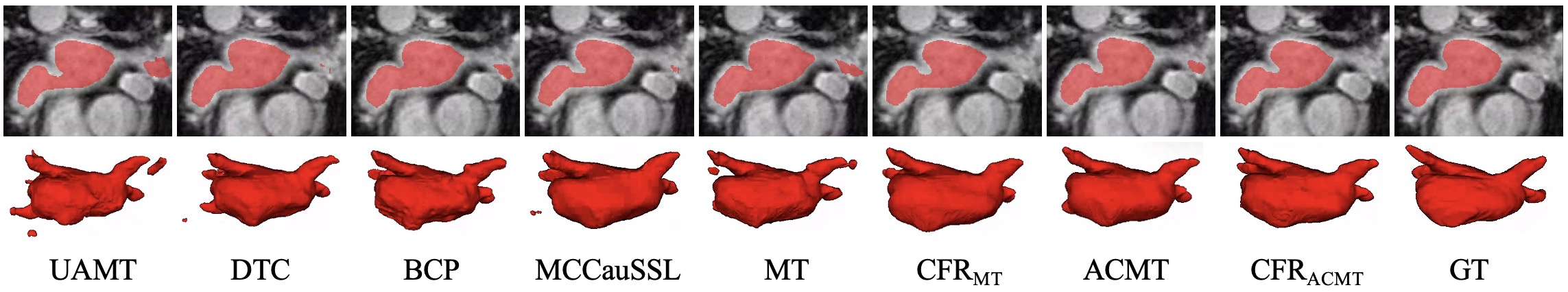
Figure 8: Segmentation results on LA dataset with 16 labeled data. GT means the ground truth.

Figure 9: Segmentation on BraTS dataset with 1 labeled data.

TABLE V: Results of BTCV dataset with moderate annotations and the evaluation metric is the Dice score (%). Note: Spl: spleen, R.Kid: right kidney, L.Kid: left kidney, Gall: gallbladder, Eso: esophagus, Liv: liver, Sto: stomach, Aor: aorta, IVC: inferior vena cava, Veins: portal and splenic veins, Pan: pancreas, LG/RG: left/right adrenal glands.

L / U	Method	AVG $\uparrow$	Spl	R.Kid	L.Kid	Gall	Eso	Liv	Sto	Aor	IVC	Veins	Pan	RG	LG
7 / 0	V-Net [26] (LB)	67.17	84.98	82.72	82.07	36.64	63.48	93.54	57.49	89.74	78.63	60.42	49.39	55.60	38.49
7 / 11	UA-MT [MICCAI’19] [12]	67.75	88.74	75.88	78.91	54.25	58.55	93.46	58.90	89.23	76.15	62.30	47.91	51.53	44.92
	CPS [CVPR’21] [15]	65.81	87.56	72.99	77.59	53.31	54.08	92.41	54.58	87.75	74.32	58.68	48.02	50.39	43.86
	ICT [NN’22] [44]	73.69	90.31	84.41	86.96	49.22	65.65	94.29	65.95	90.23	81.44	69.56	66.61	57.35	56.01
	SS-Net [MICCAI’22] [53]	58.26	84.74	76.37	74.19	43.42	57.05	92.90	14.37	83.14	69.77	52.45	27.08	54.29	27.66
	SLC-Net [MICCAI’22] [54]	70.40	90.05	84.00	86.43	56.16	58.91	94.68	70.72	89.93	79.45	60.59	54.22	51.03	39.08
	MT [NIPS’17] [13]	65.68	85.70	78.93	79.08	42.80	61.09	93.45	57.57	89.70	80.30	63.95	41.14	50.46	29.69
	CFR${}_{\text{MT}}$ (Ours)	70.09 ($\uparrow$4.41)	87.92	82.86	81.94	53.02	60.50	95.06	72.82	89.71	81.23	67.46	59.29	41.77	37.58
	MagicNet [CVPR’23] [8]	76.74	91.61	85.02	88.13	58.16	66.72	94.07	74.46	90.77	84.31	71.56	68.90	63.48	60.47
	CFR${}_{\text{MagicNet}}$ (Ours)	77.06 ($\uparrow$0.32)	92.09	85.36	83.70	63.38	69.97	94.15	74.69	91.14	84.45	70.68	67.22	64.39	60.53
18 / 0	V-Net [26] (UB)	76.28	84.00	84.82	86.38	67.42	65.02	94.83	73.75	90.27	84.19	69.85	63.54	62.60	65.02

TABLE VI: Results of MACT dataset with moderate annotations and the evaluation metric is the Dice score (%). L.Kidey: left kidney.

L / U	Method	AVG $\uparrow$	Spleen	L.Kedney	Gallbladder	Esophagus	Liver	Stomach	Pancreas	Doudenum
14 / 0	V-Net [26] (LB)	69.05	93.94	94.36	60.43	0*	95.57	78.04	72.19	57.83
14 / 56	UA-MT [MICCAI’19] [12]	78.33	93.76	92.07	75.01	65.53	95.42	77.91	72.40	54.57
	CPS [CVPR’21] [15]	65.17	93.84	79.80	64.62	0*	93.66	81.49	62.25	45.70
	ICT [NN’22] [44]	77.52	93.12	92.05	71.51	67.54	94.38	77.40	68.03	56.16
	SS-Net [MICCAI’22] [53]	69.69	93.15	92.89	71.75	0*	93.08	73.99	73.11	59.56
	MT [NIPS’17] [13]	77.10	93.52	93.06	75.19	67.61	94.44	67.99	73.39	51.56
	CFR${}_{\text{MT}}$ (Ours)	82.50 ($\uparrow$5.40)	95.77	94.42	83.61	68.92	96.05	82.81	76.30	62.10
	MagicNet [CVPR’23] [8]	81.04	94.19	94.38	76.07	74.08	95.04	78.55	73.36	62.61
	CFR${}_{\text{MagicNet}}$ (Ours)	82.87 ($\uparrow$1.83)	95.54	94.45	82.67	72.89	95.93	81.49	75.90	64.06
70 / 0	V-Net [26] (UB)	85.85	96.07	95.05	84.09	72.28	96.31	89.45	82.05	71.47

VIII-B Experimental Settings

In this paper, all the experiments are implemented in Pytorch on the NVIDIA GeForce RTX 3090/4090TI GPU. For foundation model SAM, we conduct all the experiments based on the “ViT-B” version. We adopt LoRA finetuning and the rank of LoRA is set to 4 for efficiency and performance optimization. In our experiments, we follow the current popular setting in designing mask decoder, i.e., SAMed [6] with LoRA, which modifies the segmentation head to generate masks of each class in a deterministic manner and aggregate them to final segmentation map.

For the semi-supervised network, it is trained by the SGD optimizer with an initial learning rate of 0.01. For LA and BraTS datasets, we follow the training strategy of [12, 9]. And we employ four measurements to quantitatively evaluate the segmentation performance, including Dice, Jaccard, the average surface distance (ASD), and the 95% Hausdorff Distance (HD). For BTCV and MACT datasets, we follow the implementation details of [8] and Dice as an evaluation metric for multi-organ segmentation. For fair comparison, we use official reported $\lambda$ of various baselines [12, 9, 8].

During inference, we discard fine-tuning module and new samples are directly predicted by re-training module.

VIII-C Results with Moderate Annotations

VIII-C1 Single Target Segmentation

We compare with current SOTA methods on LA dataset and BraTS dataset, including V-Net [26], MT [13], UA-MT [12], CCT [14], CPS [15], DTC [43], ICT [44], CPCL [45], URPC [46], BCP [10], MCCauSSL [17] and ACMT [9], and the results are shown in Table I and Table II. We select the basic MT [13] network and method ACMT [9] with the current highest performance, and respectively provide pseudo-labels of adapted SAM to assist training. Our CFR framework with MT and ACMT as the retraining module is denoted as CFR${}_{\text{MT}}$ and CFR${}_{\text{ACMT}}$, respectively. The results show that CFR framework brings substantial improvements in both MT and ACMT methods, approaching the performance of fully-supervised segmentation.

VIII-C2 Multiple Target Segmentation

Table V and Table VI show the results on BTCV and MACV datasets, respectively. We compare our method with V-Net [26], MT [13], UA-MT [12], CPS [15], ICT [44], SS-Net [53], SLC-Net [54], and MagicNet [8]. We employ CFR framework to guide the classical MT [13] and the SOTA MagicNet [8] methods, i.e., CFRMT and CFRMagicNet. By leveraging the CFR framework, both methods achieve significant performance improvements. On the BTCV dataset, CFRMagicNet even surpasses the results obtained with fully-supervised learning.

TABLE VII: Results of BTCV dataset with scarce annotations and the evaluation metric is the Dice score (%). Note that the full name of the organ is the same as in Table V.

L / U	Method	AVG $\uparrow$	Spl	R.Kid	L.Kid	Gall	Eso	Liv	Sto	Aor	IVC	Veins	Pan	RG	LG
1 / 0	V-Net [26] (LB)	14.84	52.97	29.59	2.34	27.63	0*	75.25	3.33	0*	0*	0*	1.87	0*	0*
1 / 17	MT [NIPS’17] [13]	29.47	67.12	41.92	41.01	0.82	0*	81.67	3.98	53.30	46.81	30.60	15.02	0*	0.82
	CFR${}_{\text{MT}}$ (Ours)	39.59 ($\uparrow$10.12)	82.87	63.52	61.20	0*	0*	87.90	19.17	81.68	61.43	33.01	23.86	0*	0*
	MagicNet [CVPR’23] [8]	40.02	52.97	50.22	44.17	10.04	35.55	76.02	29.30	56.69	49.65	37.59	48.58	16.31	13.15
	CFR${}_{\text{MagicNet}}$ (Ours)	53.59 ($\uparrow$13.57)	85.01	67.43	56.74	34.77	35.90	86.65	38.07	84.58	57.45	56.90	43.35	20.94	28.84

TABLE VIII: Results of MACT dataset with scarce annotations and the evaluation metric is the Dice score (%). L.Kidey: left kidney.

L / U	Method	AVG $\uparrow$	Spleen	L.Kedney	Gallbladder	Esophagus	Liver	Stomach	Pancreas	Doudenum
1 / 0	V-Net [26] (LB)	18.73	41.76	5.19	3.70	0.23	85.87	11.09	1.98	0.05
1 / 69	MT [NIPS’17] [13]	23.09	37.08	29.58	6.74	0*	77.41	27.65	4.78	1.49
	CFR${}_{\text{MT}}$ (Ours)	36.23 ($\uparrow$13.14)	74.41	64.11	7.37	0*	91.01	36.94	13.37	2.65
	MagicNet [CVPR’23] [8]	42.90	79.32	62.32	21.30	20.87	89.60	44.96	12.83	12.01
	CFR${}_{\text{MagicNet}}$ (Ours)	49.08 ($\uparrow$6.18)	89.57	74.00	33.21	16.55	91.05	46.91	25.84	15.47

VIII-D Results with Scarce Annotations

VIII-D1 Single Target Segmentation

We evaluate the impact of CFR with scarce annotations on the LA and BraTS datasets. In Table III, when only one labeled volume is available, supervised learning performs poorly, achieving only 17.99% accuracy. CFR takes advantage of medical image concatenation and SAM’s powerful feature capture capabilities to guide MT to increase from 29.68% to 74.40%. The results of the BraTS are shown in Table IV and CFR helps MT improve by 15.06% and MagicNet by 15.15%. In addition, one phenomenon observed is that some semi-supervised methods perform worse than the lower bound. This could be attributed to the incomplete similarity of the data distribution between labeled and unlabeled samples, and the inaccurate pseudo-labels from the unlabeled samples have a negative impact on the model’s learning process.

VIII-D2 Multiple Target Segmentation

The results of scarce annotations on two multi-organ datasets are presented in Table VII and Table VIII. On BTCV dataset with only one labeled sample, the model struggles to identify esophagus, aorta, inferior vena cava, portal and splenic veins, left and right adrenal glands, with Dice scores below 5% for left kidney, stomach, and pancreas. Semi-supervised methods with unlabeled samples alleviate the poor performance of most organs. Our CFR framework achieves improvements of 10.12% and 13.57% on MT and MagicNet models, respectively, particularly with a nearly 30% improvement on aorta region. Similarly, on MACT dataset, CFR helps identify challenging classes, with significant improvements of 37.33% for spleen and 34.53% for right kidney on the Mean Teacher model.

VIII-E Effectiveness of Re-training Module

We report the results of fine-tuning step omitting re-training in all datasets in Table IX, and compare the model parameters and performance after fine-tuning and re-training steps. By comparing fine-tuning results with re-training results in more detail, we observe that there is a slight performance decrease in CFR${}_{\text{MT}}$ with scarce labels on LA and BTCV datasets, but overall there is a clear improvement in effect. On the other hand, considering the practical deployment requirements, re-training model has a smaller number of parameters than fine-tuning model. Our fine-tuning module CFR${}_{\text{FT}}$ has the same parameter size as the foundation model (SAM) and the re-training module reduces the parameter scale to the mainstream segmenters. The results validate that the re-training module contributes to an overall performance boost for semi-supervised segmentation.

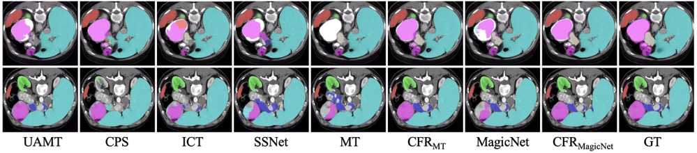
Figure 10: Segmentation results on MACT dataset with 14 labeled data. GT means the ground truth.

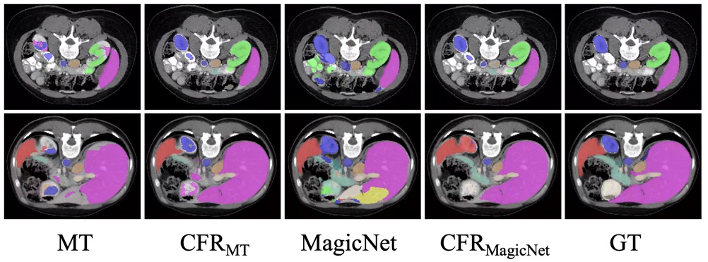
Figure 11: Segmentation on BTCV dataset with 1 labeled data.

TABLE IX: Comparison of fine-tuning and re-training segmentation results of Dice on four datasets. “# L” is the number of labeled data. ”M” means moderate and ”S” means scarce.

#L	Method	Params$\downarrow$	Dice$\uparrow$
			LA	BraTS	BTCV	MACT
M	CFR${}_{\text{FT}}$	91M	90.39	84.94	65.26	79.59
	CFR${}_{\text{MT}}$	10M	90.86	85.19	70.09	82.50
			($\uparrow$0.47)	($\uparrow$0.25)	($\uparrow$4.83)	($\uparrow$2.91)
	CFR${}_{\text{ACMT/MagicNet}}$	10/18M	90.95	85.81	77.06	82.87
			($\uparrow$0.56)	($\uparrow$0.87)	($\uparrow$11.80)	($\uparrow$3.28)
S	CFR${}_{\text{FT}}$	91M	74.78	78.14	40.98	35.13
	CFR${}_{\text{MT}}$	10M	74.40	78.58	39.59	36.23
			($\downarrow$0.38)	($\uparrow$0.44)	($\downarrow$1.39)	($\uparrow$1.10)
	CFR${}_{\text{ACMT/MagicNet}}$	10/18M	76.76	78.47	53.59	49.08
			($\uparrow$1.98)	($\uparrow$0.33)	($\uparrow$12.61)	($\uparrow$13.95)

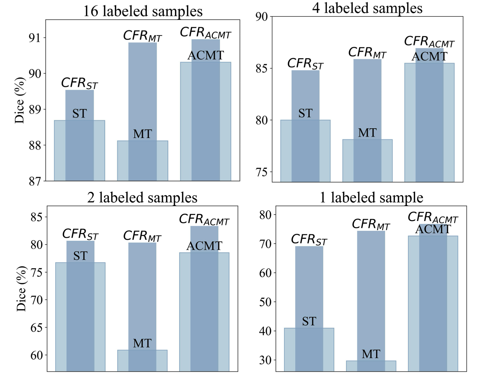
Figure 12: Results of CFR on self-training (ST in short), MT and ACMT with different numbers of labeled samples.

VIII-F Visual analysis

VIII-F1 Visualization on Moderate Annotations

The single target segmentation examples on LA dataset are shown in Figure 8, compared with current SOTA methods including MT [13], UA-MT [12], DTC [43], BCP [10], MCCauSSL [17] and ACMT [9]. Our CFR${}_{\text{MT}}$ and CFR${}_{\text{ACMT}}$ predictions align more accurately with ground truth masks, further validating the effectiveness. For multiple target datasets, we demonstrate the segmentation results of MACT dataset with 14 annotated samples in Figure 10. Our CFR${}_{\text{MT}}$ and CFR${}_{\text{MagicNet}}$ are compared with MT [13], UA-MT [12], CPS [15], ICT [44], SS-Net [53] and MagicNet [8] methods. It can be observed that our framework performs well in areas where semi-supervised methods struggle to identify, such as the stomach (magenta), pancreas (blue), and left kidney (green) regions.

VIII-F2 Visualization on Scarce Annotations

Figure 9 and 11 are the segmentation examples of single target and multiple target datasets with scarce annotations, taking the BraTS dataset and BTCV dataset as examples. The effectiveness of our proposed framework can be shown in some challenging examples. In these examples, the baselines (i.e., MT [13], ACMT [9] and MagicNet [8]) tend to generate false predictions or incomplete structures, whereas the introduction of the CFR framework can mitigate these problems and obtain a more plausible segmentation result.

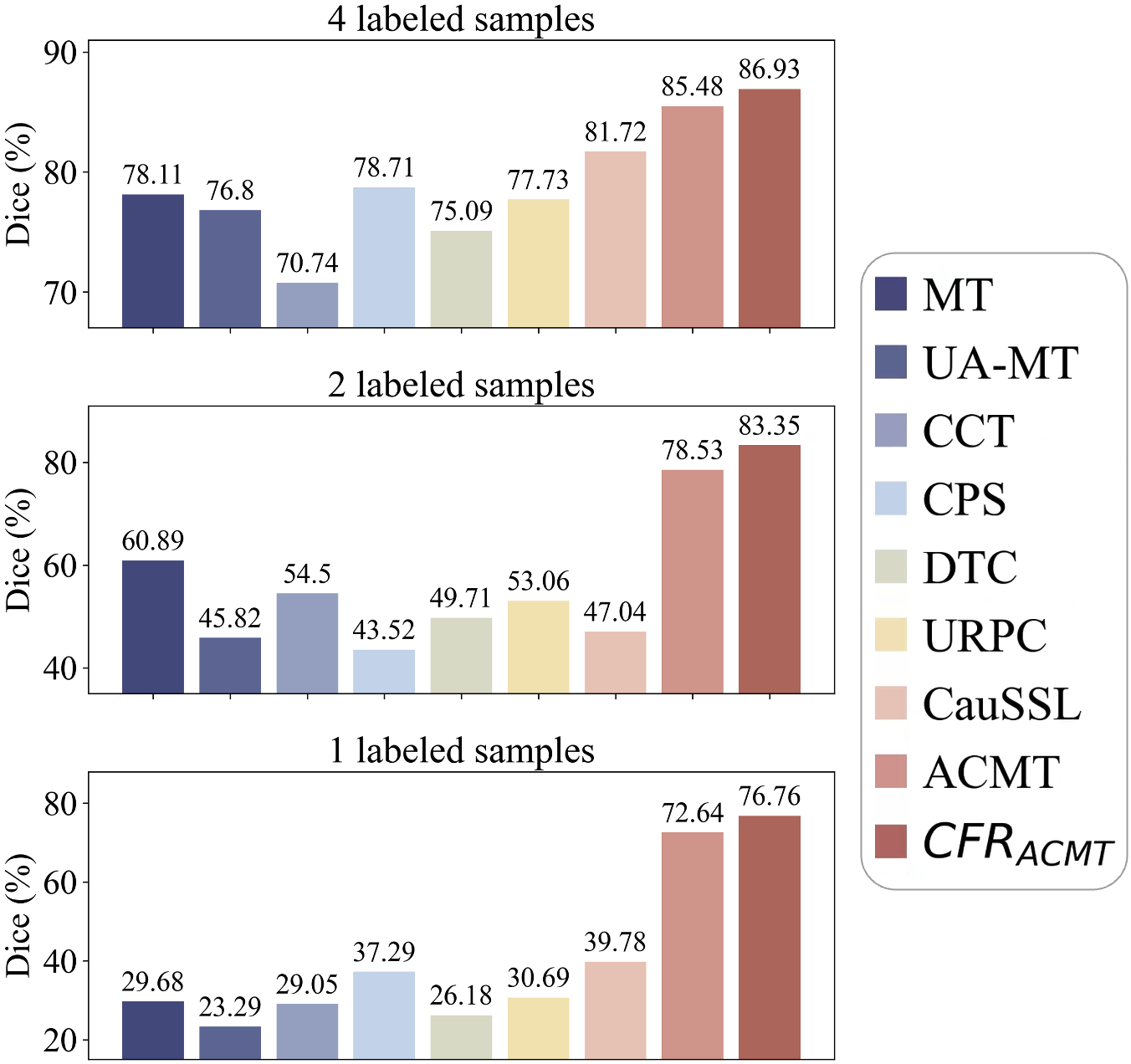
Figure 13: Comparison of different SSL methods on LA dataset with 4, 2, and 1 labeled samples.

VIII-G Further Analysis

VIII-G1 Analysis of Initial Pseudo-labels

We compare our fine-tuning module of CFR framework with four foundation model fine-tuning methods, including MedSAM-v1 [19], MedSAM-v2 [19], SAMed [6] and SAMUS [20]. MedSAM adopts a sub-parts fine-tuning approach and SAMed is a LoRA-based adapter tuning method, which maintains the same parameter scale as the original SAM model. SAMUS introduces a parallel CNN branch and thus has more parameters. As shown in Figure 1, it demonstrates that our concatenation fine-tuning strategy (denoted as CFR${}_{\text{FT}}$) achieves a significant performance improvement without introducing additional parameters, and therefore could provide more reliable pseudo-labels for subsequent retraining module.

VIII-G2 Compared with 3D-based SAM methods

We compare the results of our fine-tuning CFR${}_{\text{FT}}$ and the existing 3D-based SAM fine-tuning method (3DSAM-Adapter) in Table X, which reveals that our method achieves better accuracy without additional computational overhead.

VIII-G3 Compatibility under Different Number of Labeled Data

With its plug-and-play nature, our re-training module could apply different SSL methods. We conduct re-training experiments on self-training, MT, and ACMT methods with different numbers of labeled samples in Figure 12. Compared to the baseline, our CFR yields excellent segmentation performance with 1, 2, 4, or 16 labeled samples. Especially in the context of extreme annotation conditions, i.e., 1 labeled sample, our framework produces impressive improvements. The comparisons with other semi-supervised methods are provided in Figure 13. The results highlight the advantages of our CFR framework in leveraging limited labeled data to achieve remarkable segmentation performance.

TABLE X: Comparison of 3D-based fine-tuning method on LA dataset.

Method	Params$\downarrow$	Dice$\uparrow$	Jaccard$\uparrow$	ASD$\downarrow$	95HD$\downarrow$
3DSAM-Adapter [36]	114M	82.39	70.85	3.74	15.49
CFR${}_{\text{FT}}$	91M	90.39	82.54	1.83	6.71

VIII-G4 Spatial Structure of Medical Images

During fine-tuning, regarding the distribution gap and dimensionality mismatch, we believe the global scope of all the consecutive slices could be a bridge to link the SAM (designed for 2D natural images) and 3D medical images. As we demonstrated in Section IV, our concatenation method outperforms the listed alternatives, indicating that in the fine-tuning step, SAM benefits from accurately locating the regions to segment due to its generalization ability in various segmentation tasks. During re-training, we still use 3D structure-based SSL methods, to retain spatial information. In a nutshell, SAM in fine-tuning and SSL in re-training separately treat 3D information in different ways: SAM to solve concatenated large-sized 2D slices, and SSL to further segment the 3D volumes.

IX Conclusion

In this work, we present the CFR framework, which consists of the concatenate, fine-tuning, and re-training modules, to achieve higher improvements in semi-supervised segmentation tasks by leveraging the foundation model. The concatenate module copes with the resolution difference between medical and natural images, and fine-tuning module provides reliable initial pseudo-labels for re-training module. Our framework maintains the same parameter size as the mainstream segmenter, e.g., V-Net [26], and could be compatible with most popular SSL methods, e.g., Mean Teacher [13]. Extensive experiments demonstrate the CFR framework improves the performance remarkably in both moderate annotation and scarce annotation scenarios.

References

- [1] X. Wang, X. Zhang, Y. Cao, W. Wang, C. Shen, and T. Huang, “Seggpt: Towards segmenting everything in context,” in ICCV, October 2023, pp. 1130–1140.
- [2] X. Zou, J. Yang, H. Zhang, F. Li, L. Li, J. Wang, L. Wang, J. Gao, and Y. J. Lee, “Segment everything everywhere all at once,” NIPS, vol. 36, 2023.
- [3] A. Kirillov, E. Mintun, N. Ravi, H. Mao, C. Rolland, L. Gustafson, T. Xiao, S. Whitehead, A. C. Berg, W.-Y. Lo et al., “Segment anything,” in ICCV, 2023, pp. 4015–4026.
- [4] A. Khani, S. Asgari, A. Sanghi, A. M. Amiri, and G. Hamarneh, “SLiMe: Segment like me,” in ICLR, 2024.
- [5] J. Wu, R. Fu, H. Fang, Y. Liu, Z. Wang, Y. Xu, Y. Jin, and T. Arbel, “Medical SAM Adapter: Adapting segment anything model for medical image segmentation,” arXiv preprint arXiv:2304.12620, 2023.
- [6] K. Zhang and D. Liu, “Customized segment anything model for medical image segmentation,” arXiv preprint arXiv:2304.13785, 2023.
- [7] Z. Xiong, Q. Xia, Z. Hu, N. Huang, C. Bian, Y. Zheng, S. Vesal, N. Ravikumar, A. Maier, X. Yang et al., “A global benchmark of algorithms for segmenting the left atrium from late gadolinium-enhanced cardiac magnetic resonance imaging,” Medical Image Analysis, vol. 67, p. 101832, 2021.
- [8] D. Chen, Y. Bai, W. Shen, Q. Li, L. Yu, and Y. Wang, “MagicNet: Semi-supervised multi-organ segmentation via magic-cube partition and recovery,” in CVPR, 2023, pp. 23 869–23 878.
- [9] Z. Xu, Y. Wang, D. Lu, X. Luo, J. Yan, Y. Zheng, and R. K.-y. Tong, “Ambiguity-selective consistency regularization for mean-teacher semi-supervised medical image segmentation,” Medical Image Analysis, vol. 88, p. 102880, 2023.
- [10] Y. Bai, D. Chen, Q. Li, W. Shen, and Y. Wang, “Bidirectional copy-paste for semi-supervised medical image segmentation,” in CVPR, 2023, pp. 11 514–11 524.
- [11] L. Wu, L. Fang, X. He, M. He, J. Ma, and Z. Zhong, “Querying labeled for unlabeled: Cross-image semantic consistency guided semi-supervised semantic segmentation,” IEEE TPAMI, 2023.
- [12] L. Yu, S. Wang, X. Li, C.-W. Fu, and P.-A. Heng, “Uncertainty-aware self-ensembling model for semi-supervised 3D left atrium segmentation,” in MICCAI. Springer, 2019, pp. 605–613.
- [13] A. Tarvainen and H. Valpola, “Mean teachers are better role models: Weight-averaged consistency targets improve semi-supervised deep learning results,” NIPS, vol. 30, 2017.
- [14] Y. Ouali, C. Hudelot, and M. Tami, “Semi-supervised semantic segmentation with cross-consistency training,” in CVPR, 2020, pp. 12 674–12 684.
- [15] X. Chen, Y. Yuan, G. Zeng, and J. Wang, “Semi-supervised semantic segmentation with cross pseudo supervision,” in CVPR, 2021, pp. 2613–2622.
- [16] Y. Wang, B. Xiao, X. Bi, W. Li, and X. Gao, “MCF: Mutual correction framework for semi-supervised medical image segmentation,” in CVPR, 2023, pp. 15 651–15 660.
- [17] J. Miao, C. Chen, F. Liu, H. Wei, and P.-A. Heng, “CauSSL: Causality-inspired semi-supervised learning for medical image segmentation,” in ICCV, 2023, pp. 21 426–21 437.
- [18] F. Wu and X. Zhuang, “Minimizing estimated risks on unlabeled data: a new formulation for semi-supervised medical image segmentation,” IEEE TPAMI, vol. 45, no. 5, pp. 6021–6036, 2022.
- [19] J. Ma, Y. He, F. Li, L. Han, C. You, and B. Wang, “Segment anything in medical images,” Nature Communications, vol. 15, no. 1, p. 654, 2024.
- [20] X. Lin, Y. Xiang, L. Zhang, X. Yang, Z. Yan, and L. Yu, “SAMUS: Adapting segment anything model for clinically-friendly and generalizable ultrasound image segmentation,” arXiv preprint arXiv:2309.06824, 2023.
- [21] J. Zhang, H. Peng, K. Wu, M. Liu, B. Xiao, J. Fu, and L. Yuan, “Minivit: Compressing vision transformers with weight multiplexing,” in CVPR, 2022, pp. 12 145–12 154.
- [22] T. Chen, Z. Zhang, Y. Cheng, A. Awadallah, and Z. Wang, “The principle of diversity: Training stronger vision transformers calls for reducing all levels of redundancy,” in CVPR, 2022, pp. 12 020–12 030.
- [23] A. Aghajanyan, L. Zettlemoyer, and S. Gupta, “Intrinsic dimensionality explains the effectiveness of language model fine-tuning,” arXiv preprint arXiv:2012.13255, 2020.
- [24] L. Alzubaidi, M. Al-Amidie, A. Al-Asadi, A. J. Humaidi, O. Al-Shamma, M. A. Fadhel, J. Zhang, J. Santamaría, and Y. Duan, “Novel transfer learning approach for medical imaging with limited labeled data,” Cancers, vol. 13, no. 7, p. 1590, 2021.
- [25] R. Jiao, Y. Zhang, L. Ding, B. Xue, J. Zhang, R. Cai, and C. Jin, “Learning with limited annotations: a survey on deep semi-supervised learning for medical image segmentation,” Computers in Biology and Medicine, p. 107840, 2023.
- [26] F. Milletari, N. Navab, and S.-A. Ahmadi, “V-net: Fully convolutional neural networks for volumetric medical image segmentation,” in 2016 fourth International Conference on 3D vision (3DV). IEEE, 2016, pp. 565–571.
- [27] S. Liu, Z. Zeng, T. Ren, F. Li, H. Zhang, J. Yang, C. Li, J. Yang, H. Su, J. Zhu et al., “Grounding dino: Marrying dino with grounded pre-training for open-set object detection,” arXiv preprint arXiv:2303.05499, 2023.
- [28] Y. Liu, J. Zhang, Z. She, A. Kheradmand, and M. Armand, “SAMM (Segment Any Medical Model): A 3d slicer integration to sam,” arXiv preprint arXiv:2304.05622, 2023.
- [29] T. Wald, S. Roy, G. Koehler, N. Disch, M. R. Rokuss, J. Holzschuh, D. Zimmerer, and K. Maier-Hein, “Sam. md: Zero-shot medical image segmentation capabilities of the segment anything model,” in MIDL, short paper track, 2023.
- [30] V. I. Butoi*, J. J. G. Ortiz*, T. Ma, M. R. Sabuncu, J. Guttag, and A. V. Dalca, “Universeg: Universal medical image segmentation,” ICCV, 2023.
- [31] Z. Huang, H. Wang, Z. Deng, J. Ye, Y. Su, H. Sun, J. He, Y. Gu, L. Gu, S. Zhang et al., “Stu-net: Scalable and transferable medical image segmentation models empowered by large-scale supervised pre-training,” arXiv preprint arXiv:2304.06716, 2023.
- [32] J. Cheng, J. Ye, Z. Deng, J. Chen, T. Li, H. Wang, Y. Su, Z. Huang, J. Chen, L. Jiang et al., “SAM-Med2D,” arXiv preprint arXiv:2308.16184, 2023.
- [33] H. Wang, S. Guo, J. Ye, Z. Deng, J. Cheng, T. Li, J. Chen, Y. Su, Z. Huang, Y. Shen et al., “SAM-Med3D,” arXiv preprint arXiv:2310.15161, 2023.
- [34] Y. Huang, X. Yang, L. Liu, H. Zhou, A. Chang, X. Zhou, R. Chen, J. Yu, J. Chen, C. Chen et al., “Segment anything model for medical images?” Medical Image Analysis, vol. 92, p. 103061, 2024.
- [35] M. A. Mazurowski, H. Dong, H. Gu, J. Yang, N. Konz, and Y. Zhang, “Segment anything model for medical image analysis: an experimental study,” Medical Image Analysis, vol. 89, p. 102918, 2023.
- [36] S. Gong, Y. Zhong, W. Ma, J. Li, Z. Wang, J. Zhang, P.-A. Heng, and Q. Dou, “3dsam-adapter: Holistic adaptation of sam from 2d to 3d for promptable medical image segmentation,” arXiv preprint arXiv:2306.13465, 2023.
- [37] E. J. Hu, Y. Shen, P. Wallis, Z. Allen-Zhu, Y. Li, S. Wang, L. Wang, and W. Chen, “LoRA: Low-rank adaptation of large language models,” in ICLR, 2022.
- [38] D.-H. Lee et al., “Pseudo-label: The simple and efficient semi-supervised learning method for deep neural networks,” in Workshop on challenges in representation learning, ICML, vol. 3, no. 2. Atlanta, 2013, p. 896.
- [39] W. Bai, O. Oktay, M. Sinclair, H. Suzuki, M. Rajchl, G. Tarroni, B. Glocker, A. King, P. M. Matthews, and D. Rueckert, “Semi-supervised learning for network-based cardiac MR image segmentation,” in MICCAI. Springer, 2017, pp. 253–260.
- [40] K. Chaitanya, E. Erdil, N. Karani, and E. Konukoglu, “Local contrastive loss with pseudo-label based self-training for semi-supervised medical image segmentation,” Medical Image Analysis, vol. 87, p. 102792, 2023.
- [41] M. Everingham, L. Van Gool, C. K. I. Williams, J. Winn, and A. Zisserman, “The PASCAL Visual Object Classes Challenge 2012 (VOC2012) Results,” http://www.pascal-network.org/challenges/VOC/voc2012/workshop/index.html.
- [42] N. Houlsby, A. Giurgiu, S. Jastrzebski, B. Morrone, Q. De Laroussilhe, A. Gesmundo, M. Attariyan, and S. Gelly, “Parameter-efficient transfer learning for NLP,” in ICML. PMLR, 2019, pp. 2790–2799.
- [43] X. Luo, J. Chen, T. Song, and G. Wang, “Semi-supervised medical image segmentation through dual-task consistency,” in AAAI, vol. 35, no. 10, 2021, pp. 8801–8809.
- [44] V. Verma, K. Kawaguchi, A. Lamb, J. Kannala, A. Solin, Y. Bengio, and D. Lopez-Paz, “Interpolation consistency training for semi-supervised learning,” Neural Networks, vol. 145, pp. 90–106, 2022.
- [45] Z. Xu, Y. Wang, D. Lu, L. Yu, J. Yan, J. Luo, K. Ma, Y. Zheng, and R. K.-y. Tong, “All-around real label supervision: Cyclic prototype consistency learning for semi-supervised medical image segmentation,” IEEE JBHI, vol. 26, no. 7, pp. 3174–3184, 2022.
- [46] X. Luo, G. Wang, W. Liao, J. Chen, T. Song, Y. Chen, S. Zhang, D. N. Metaxas, and S. Zhang, “Semi-supervised medical image segmentation via uncertainty rectified pyramid consistency,” Medical Image Analysis, vol. 80, p. 102517, 2022.
- [47] Ö. Çiçek, A. Abdulkadir, S. S. Lienkamp, T. Brox, and O. Ronneberger, “3D U-Net: learning dense volumetric segmentation from sparse annotation,” in MICCAI. Springer, 2016, pp. 424–432.
- [48] B. H. Menze, A. Jakab, S. Bauer, J. Kalpathy-Cramer, K. Farahani, J. Kirby, Y. Burren, N. Porz, J. Slotboom, R. Wiest et al., “The multimodal brain tumor image segmentation benchmark (BRATS),” IEEE TMI, vol. 34, no. 10, pp. 1993–2024, 2014.
- [49] S. Bakas, H. Akbari, A. Sotiras, M. Bilello, M. Rozycki, J. S. Kirby, J. B. Freymann, K. Farahani, and C. Davatzikos, “Advancing the cancer genome atlas glioma MRI collections with expert segmentation labels and radiomic features,” Scientific data, vol. 4, no. 1, pp. 1–13, 2017.
- [50] S. Bakas, M. Reyes, A. Jakab, S. Bauer, M. Rempfler, A. Crimi, R. T. Shinohara, C. Berger, S. M. Ha, M. Rozycki et al., “Identifying the best machine learning algorithms for brain tumor segmentation, progression assessment, and overall survival prediction in the BRATS challenge,” arXiv preprint arXiv:1811.02629, 2018.
- [51] B. Landman, Z. Xu, J. Igelsias, M. Styner, T. Langerak, and A. Klein, “Miccai multi-atlas labeling beyond the cranial vault–workshop and challenge,” in Proc. MICCAI Multi-Atlas Labeling Beyond Cranial Vault—Workshop Challenge, vol. 5, 2015, p. 12.
- [52] E. Gibson, F. Giganti, Y. Hu, E. Bonmati, S. Bandula, K. Gurusamy, B. Davidson, S. P. Pereira, M. J. Clarkson, and D. C. Barratt, “Automatic multi-organ segmentation on abdominal ct with dense v-networks,” IEEE TMI, vol. 37, no. 8, pp. 1822–1834, 2018.
- [53] Y. Wu, Z. Wu, Q. Wu, Z. Ge, and J. Cai, “Exploring smoothness and class-separation for semi-supervised medical image segmentation,” in MICCAI. Springer, 2022, pp. 34–43.
- [54] J. Liu, C. Desrosiers, and Y. Zhou, “Semi-supervised medical image segmentation using cross-model pseudo-supervision with shape awareness and local context constraints,” in MICCAI. Springer, 2022, pp. 140–150.