Dynamics of two by two symmetric matrices of trace zero
Arijit Mukherjee
Department of Mathematics, Indian Institute of Science Education and Research Tirupati, Karakambadi Rd, opp. Sree Rama Engineering College, Rami Reddy Nagar, Mangalam, Tirupati, Andhra Pradesh - 517 507, India.
mukherjee90.arijit@gmail.com
Abstract.
In this paper, we describe the entire structure of the vector space of all symmetric matrices of size having trace zero. This is motivated by the geometrical interpretation of any arbitrary element of . We further study the orbits and stable sets of these elements. As an application of the obtained structure of , we obtain the symmetric matrices of size , trace of whose product with any trace zero symmetric matrix is zero. Finally some well known trigonometric formulas are interpreted geometrically incorporating the anatomy of .
The study of symmetric matrices and trace zero matrices attracted considerable attention. Many mathematicians have researched on symmetric matrices to study SNIEP, symmetric non-negative inverse eigenvalue problem (cf. [2],[5],[6] & [7]). Also people have independently worked on trace zero matrices and found necessary and sufficient conditions for a matrix to have zero trace (cf. [1] & [8]). A study of SNIEP for trace zero symmetric matrices can be found in [9].
This paper is devoted to the study of trace zero symmetric matrices of size and its applications. But we do it in a different context and therefore follow a different approach altogether.
We begin by fixing some notations which we are going to use repeatedly. Let be the field of real numbers. In this paper, by a vector space we always mean a vector space over and by a matrix we mean a matrix with real entries. Let & be the set of all symmetric matrices and orthogonal matrices of size respectively and be the subset of consisting of all matrices having trace zero. By we denote the set of all symmetric matrices, trace of whose product with any element of is zero. We reserve the notations and for identity matrix and zero matrix of size respectively. We denote the trace of a given matrix by and determinant of by . Given any two matrices and of size , we denote the matrix multiplication simply by their juxtaposition .
In this paper, our main aim is to describe the precise structure of . In Theorem 2.3, we show that the elements of are precisely of the form for some . Using the structure of , we further show that the set of all trace zero symmetric matrices of size having eigenvalues and is same as the set of all size orthogonal matrices having determinant , (cf. Corollary 2.4).
We come up with the geometrical interpretation of the elements of as well. In fact, this is the motivation behind finding the anatomy of . Moreover, we extensively discuss about the orbits, raise the questions about the finiteness of those orbits and answer those using the obtained structure of . We obtain a necessary and sufficient condition for finiteness of the orbit of an arbitrary element of starting at a point (cf. Theorem 2.6).
We also study the dynamics of and show how the stable set of any point with respect to varies as varies. In the process, we obtain that the stable set either contains only or is the whole of depending on whether lies in the open interval or not, (cf. Theorem 2.9).
In section 3, we look upon a couple of applications of the structure of . Firstly, we derive the structure of in subsection 3.1. To be precise, we show that consists of scalar matrices and scalar matrices only, (cf. Theorem 3.1). We then prove that the obtained anatomy of can be generalised for any using Frobenius inner product on (cf. Theorem 3.2).
As another application, we talk about two rigid motions, namely rotation and reflection, of any point of the Euclidean plane and show that rotating the point of reflection of a given point with respect to a line is same as reflecting it with respect to some other line, (cf. Theorem 3.3). Though this can be proved using simple techniques of Euclidean geometry, but we do it incorporating the structure of and as a result the elucidation seems to be an elegant one. The given proof can also be thought of as a geometric interpretation of couple of well known and frequently used trigonometric formulas (cf. Remark 3.4).
In Section 4, we conclude by indicating that the structure of some subsets of can be obtained for as well by adapting the method used in Theorem 2.3, provided some conditions being suitably put on the set of eigenvalues of its elements.
2. On the structure of and orbits of its elements
In this section, we provide the structure of , analyse its elements from a geometric viewpoint and then discuss upon the orbits and the stable sets of those elements.
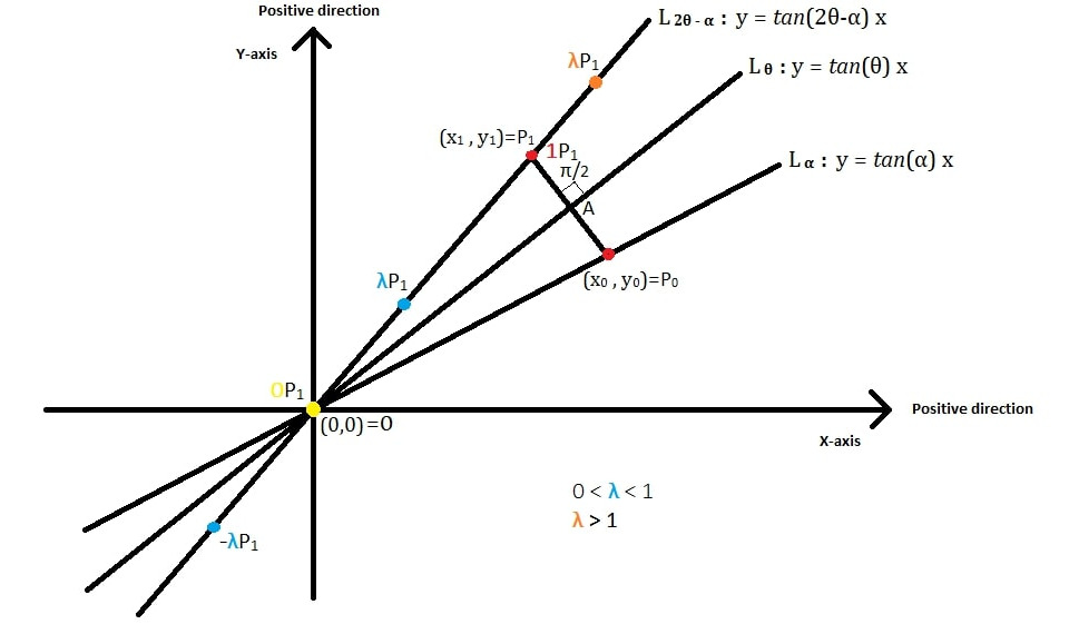
For any given real number , denote the line in passing through origin and making an angle with the positive direction of -axis in the anticlockwise direction by . Given any , define a map (geometrically), denoted by , as follows : Given any point , the map first reflects the point with respect to the line and scales that by followed by that. Denoting the reflection of with respect to the line by , the map can be given as follows:
(1)
Define the orbit of the map starting at a point as follows:
We now ask the following questions:
Questions.
(1)
Given any , for what values of and ,the orbit is finite?
(2)
For what values of and , the orbit is a singleton set, where ?
(3)
Given any , for what values of and , the orbit is a set having two points?
(4)
For what values of and , for some positive integer ?
(5)
Given any , the sequence is convergent in usual topology and in discrete topology for what values of and ?
To answer these questions, we first calculate for any given point . We do the calculation assuming that both the coordinates of the point are positive and the line joining and origin makes an angle with the positive direction of -axis. That is to say, lies in the line . Moreover, we assume that , that is to say the lines , and are having slopes in non-decreasing order, lies in first and third quadrant and none of those are -axis or -axis. The calculations are very much similar in the remaining cases as well.
As we mentioned, we start with a point lying in the line . We first want to determine the reflection of with respect to the line . For that we draw a perpendicular from the point to the line and denote the point of intersection of this with by . Then we extend the line segment and suppose that intersects the line at the point . Then clearly the point is the reflection of . Now we determine and in terms of the known quantities , , and using the properties of reflection.
Figure 1. Image of a point under the map for some values of
The equations of the line , and are given as follows:
By properties of reflection, we get that the triangle and are congruent to each other. That is to say, . Therefore, the length of the line segment is equal to that of , that is to say, . We then have the following implications.
So the abscissa of the point of reflection of is given as follows:
(2)
As lies in the line , we have . We now have the following implications:
So the ordinate of the point of reflection of is given as follows:
(3)
Remark 2.1.
Taking in equations (2) and (3), we have . On the other hand, if and , then as and . This can be justified also using (2) and (3). This depicts the fact that reflection of any point located on the axis of the reflection is the point itself. Moreover, this is true exclusively for points located on the line of reflection.
So we have obtained the coordinates of the point of reflection of about the line . For the moment, we take a break from the discussion about the map . We continue with the same after a while and answer the questions raised.
We now provide the description of . Towards that, we have the following proposition which says about the structure of the set of orthogonal matrices of size . Though this is a standard result (for example, see [3, p. 348] for determinant orthogonal matrices), we include this over here for the sake of continuity.
Proposition 2.2.
The collection of all orthogonal matrices of size is given as follows:
Proof.
Given and , by we denote the standard inner product of and in . That is to say, . Let be a given orthogonal matrix. As the columns of are of unit norm with respect to the standard inner product of , we have
As the columns of are orthogonal with respect to the standard inner product of , we have
(6)
Case - 1:
If , then we moreover have
(7)
So, conditions (5), (6) and (7) imply that, there exists such that
(8)
Case - 2:
If , then we moreover have
(9)
So, conditions (5), (6) and (9) imply that, there exists such that
(10)
Therefore, we have the result from (8) and (10).
∎
Following theorem describes the entire structure of .
Theorem 2.3.
The collection of all trace zero symmetric matrices of size is given as follows:
Proof.
By spectral theorem, we have that any real symmetric matrix is orthogonally diagonalisable and vice versa (cf. [3, p.347]). That is, for , given any symmetric matrix , there exists an orthogonal matrix such that
(11)
Moreover, if then sum of eigenvalues of is zero, that is, .
Case - 1:
If , then by Proposition 2.2 there exists such that . So, we also have .
Therefore, from (11) we have the following:
Case - 2:
If , then by Proposition 2.2 there exists such that . So, we also have .
Therefore, from (11) we have the following:
By taking if & if in Case - 1 and if & if in Case - 2, we have the theorem.
∎
We get the following obvious conclusion relating orthogonal matrices of size having determinant and a subset of .
Corollary 2.4.
Any orthogonal matrix of determinant is a symmetric matrix of trace zero. Moreover, given any symmetric matrix of trace zero, there exists a orthogonal matrix of determinant and a scalar such that . Furthermore, the set of all trace zero symmetric matrices of size having eigenvalues and is same as the set of all size orthogonal matrices having determinant .
Proof.
Follows directly from Proposition 2.2 and Theorem 2.3.
∎
We now resume the discussion about the map . We did some calculations and obtained the coordinates of the point of a given point with respect to the line . Look at the same calculations from a different point of view. Consider the matrix . Then
Recall the definition of the map as defined in (1). Now treating points of as column vectors, from (15) we can conclude that
Moreover,
(16)
Thus, (16) provides the geometry of the elements of . Also from now on we simply use the notation to mean both and if there is there is no confusion regarding the line of reflection . So, and denote the same map and we use them interchangeably.
We now answer the questions we posed related to the map . Towards that, we have the following proposition.
Proposition 2.5.
Let be any positive integer. Then
if and only if is even and or .
Proof.
It is easy to observe that . Therefore, if is even and or , then .
Conversely, let . Therefore,
(17)
Recall that . Now if is odd, then (17) implies that , which in turn says that . This contradicts (17). Therefore if then can’t be odd. Hence is even and moreover by (17) or .
∎
Now we are in a position to find some exclusive conditions which will force the orbit to be finite. Precisely, we obtain the following.
Theorem 2.6.
Let be any non-zero real number and let be any point of other than origin. Then is finite if and only if or .
Proof.
We first show that to get the finiteness of the orbit it is sufficient to have or . For that, we proceed contra positively.
We now prove the converse part. Let is finite. Then
(18)
Now if is even, then by (18) we further have the following implications.
For odd, we further consider two mutually exclusive and exhaustive cases.
First Case - :
By (18) we have the following implications.
Second Case - :
Let for some real number . As is odd, by (18), we have that , where one of and is odd and other is even. Without loss of generality, take to be odd and to be even. Then we have . Therefore, and are collinear, which is a contradiction to the assumption that by Remark 2.1. So, this case is not at all feasible.
∎
Remark 2.7.
(1)
Theorem 2.6 talks about a necessary and sufficient condition for finiteness of the orbit for non-zero values of and for points . Also, is finite if either or .
(2)
We now check when is either singleton or consists of two elements.
(a)
If , then for all and .
(b)
If , then we have the following:
(i)
If , then .
(ii)
If , then and .
(iii)
.
So, we discussed a few cases where the orbit is either singleton or consists of two elements only. It can be easily checked that these are all possible such orbits.
We now look at the sequence . We want to find some suitable , and such that the sequence is eventually constant. At this point, we note that whenever the sequence is eventually constant, the orbit must be finite. Therefore, can have only three values, namely , and unless we take (cf. Theorem 2.6 and Remark 2.7). If we take , then for any and , is a constant sequence having all the terms equal to . So look at points other than origin. Let lies in the line for some . Then clearly the sequence is eventually constant. For , is eventually constant only when . Finally provides us eventually constant sequences only in the most simplest case, that is, when . As in the discrete topology on , only convergent sequences are the eventually constant ones, therefore the sequence is convergent in discrete topology in the following cases. The point of convergence is also given accordingly.
(1)
When , the sequence converges to in discrete topology, for any and .
(2)
When , the sequence converges to in discrete topology, for any and .
(3)
When , the sequence converges to in discrete topology for any if .
As discrete topology is finer than usual topology on , the mentioned sequences are convergent in usual topology as well. We now find out whether there are some more sequences that are convergent in usual topology. As the metric induced by the usual topology on is a complete metric, to find out the convergent sequences it is enough to find the Cauchy sequences over there.
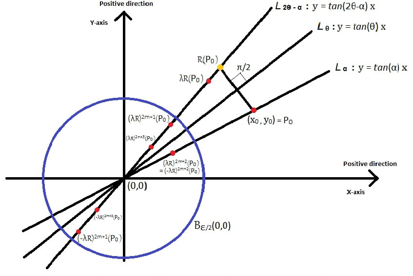
We observe that for any , if for some , , then . As the lines and intersect only at origin, the distance between any two consecutive terms of the sequence can be made arbitrarily small, that is, the sequence can be made to be a Cauchy sequence, only when the terms of the sequence approach origin. So we conclude that the only possible point of convergence of the sequence , with infinitely many distinct terms, is . We claim that this only possibility can be attained by the sequence for all non-zero with .
Recall that when is even and when is odd. Using this we calculate some upper bounds of the distances between terms of the sequence . Here by distance between any two points and of , we mean the Euclidean distance between them and denote that by .
Case 1 : When both and are even
(19)
Case 2 : When both and are odd
(20)
Case 3 : When is even and is odd
(21)
So given any , by (19), (20) and (21), we can choose such that for all , whenever . Therefore, the sequence is a Cauchy sequence for all with and hence convergent to in usual topology as we justified earlier that is the only possible point of convergence.
Figure 2. Convergence of the sequence for
Also, it can be directly checked that the sequence converges to for all with .
Case 1 : When is even
(22)
Case 2 : When is odd
(23)
So given any , by (22) and (23), we can choose such that for all , whenever . Therefore, for all with , the terms of the sequence eventually lie in the open ball of radius and having centre at and hence convergent to in usual topology.
We want to summarize what we have discussed so far regarding the convergence of the sequence from a different perspective. For that we lend some terminologies from dynamical systems and define those solely in our context.
Definition 2.8.
Let be a finite dimensional vector space over and be a metric on . Also let be a linear map. Then any two points , of are said to be forward asymptomatic with respect to the map if as . For any , the stable set of with respect to , denoted by , is the set of all points forward asymptomatic to with respect to .
We now have the following theorem regarding how the stable set of any point of with respect to any arbitrary element of changes all of a sudden as varies from to .
Theorem 2.9.
Consider the metric space where denotes the usual metric. Then the following hold for any point :
(1)
For any with ,
(2)
For any with ,
Proof.
For any and for any odd ,
(24)
Also for any and even ,
(25)
Therefore we have the following as varies.
(1)
For all , as by (24) and (25), whenever . So any point of is forward asymptomatic to and hence .
(2)
By (24) and (25), for , as if and only if if and only if . So the only point forward asymptomatic to is itself, that is to say .
∎
Remark 2.10.
First part of Theorem 2.9 can be proved alternatively as follows. We first claim that for any with . When , it is easy to see that any point of is forward asymptomatic to with respect to . Also, the same is true for any with by (22) and (23). Hence we have the claim. Now for any point ,
Therefore for all , as by (22) and (23). So any point of is forward asymptomatic to and hence .
3. Applications of the structure of
In this section we talk about a couple of applications of the obtained structure of . In the first subsection we obtain the structure of the set . In the next subsection we reinterpret some trigonometric formulas and show how those can be used to solve purely geometric questions.
3.1. The structure of
Recall that is the set of all symmetric matrices, trace of whose product with any element of is zero. In this subsection we obtain the structure of in the form of following theorem.
Theorem 3.1.
The set is the set of all scalar matrices of size .
Proof.
Let be arbitrarily chosen. Then for all . Therefore by Theorem 2.3, we have:
for all and . That is, for all and ,
(26)
Plugging and in (26), we get . Similarly, plugging and in (26), we get . Hence, the assertion follows.
∎
In fact, we have the following more general result. This is motivated by [4, Problem 9, Exercises VI, S2, p.190].
Theorem 3.2.
For any positive integer , is the set of all scalar matrices of size .
Proof.
Consider the Frobenius inner product on given by , for any . Then is nothing but the orthogonal complement of with respect to the Frobenius inner product. Now as is a subspace of of co-dimension and as , we have the theorem.
∎
So, the proof of Theorem 3.1 incorporates the obtained structure of and provides an alternative way of proving Theorem 3.2 for .
3.2. Interpreting some trigonometric formulas
In this subsection, we prove an interesting geometric property of using the geometric interpretation of the elements of (cf. (16)). Precisely, we prove the following :
Theorem 3.3.
Given any real number , let denotes the line passing through origin and making an angle (in the anticlockwise direction) with positive direction of axis. Then, given any point of , rotating the point of reflection of clockwise (respectively anticlockwise) with respect to the line by an angle is same as reflecting with respect to the line (respectively ).
Proof.
We interpret a point of as the column vector . From (1), (16) and Theorem 2.3, we have that an element of , denoted by , reflects a point with respect to the line . An orthogonal matrix of determinant , denoted by , represents clockwise rotation of the plane . Similarly, the matrix represents anticlockwise rotation of the plane (cf. [3, p.348]). Hence, to prove the theorem, we need to show that for clockwise case and for anticlockwise case. Now,
(27)
Similarly we have :
(28)
The theorem now follows from (27) and (28) for clockwise and anticlockwise scenario respectively.
∎
Remark 3.4.
Theorem 3.3 talks about a geometric property of the plane in both clockwise and anticlockwise context. Let’s denote that property by for clockwise case and by for anticlockwise case. Now consider the following standard trigonometric equalities :
(29)
(30)
So, Theorem 3.3 says that can be thought of as a geometric interpretation of the equalities in (30) (cf. (27)). Similarly, deciphering (29) geometrically, we obtain (cf. (28)).
4. Conclusion
It is worth mentioning that the structure of some subsets of can be obtained for as well by adapting the method used in Theorem 2.3, provided some conditions being suitably put on the set of eigenvalues (other than they add upto zero) of all its elements.
5. Acknowledgements
The author wishes to thank Indian Institute of Science Education and Research Tirupati (Award No. - IISER-T/Offer/PDRF/A.M./M/01/2021) for financial support. The author is grateful to the referee for several valuable comments.
References
[1] Albert, A. A. and Muckenhoupt, B., On matrices of trace zeros, Michigan Math. J., 4 (1957), 1–3.
[2] Fiedler, M., Eigenvalues of nonnegative symmetric matrices, Linear Algebra Appl., 9 (1974), 119–142.
[3] Herstein, I. N., Topics in algebra, 2nd ed. Lexington: Xerox College Publishing, 1975.
[4] Lang, S., Linear algebra, Inc.:Reading: Addison-Wesley Publishing Co., 1966.
[5] Loewy, R. and London, D., A note on an inverse problem for nonnegative matrices, Linear and Multilinear Algebra, 6 (1978), 83–90.
[6] Loewy, R., and McDonald, J. J., The symmetric nonnegative inverse eigenvalue problem for matrices, Linear Algebra Appl.393 (2004), 275–298.
[7] McDonald, J. J. and Neumann, M., The Soules approach to the inverse eigenvalues problem for nonnegative symmetric matrices of order , Contemp. Math., 259 (2000), 387–407.
[8] Shoda, K., Einige Sätze über Matrizen, Jpn. J. Math., 13(3) (1937), 361–365.
[9] Spector, O., A characterization of trace zero symmetric nonnegative matrices, Linear Algebra Appl., 434(4) (2011), 1000–1017.