From habitat decline to collapse: a spatially explicit approach connecting habitat degradation to destruction

Abstract

Habitat loss, through degradation and destruction of viable habitat, has a well-documented and undeniable impact on the sustainability of ecosystems [12, 40, 41]. Moreover, most habitat loss is anthropogenic [31]. Understanding the relationships between varying degrees of habitat degradation, movement strategies, and population dynamics on species persistence is crucial. We establish a robust connection between habitat degradation and destruction using a reaction-diffusion equation framework. Motivated by the recent work [43], we consider an intrinsic growth rate function that features a logistic-type growth in the viable habitat but decays at rate $c\geq 0$ in the degraded region(s). In the limit as $c\to\infty$, the solution to the habitat degradation problem converges uniformly to the solution of a related habitat destruction problem. When the habitat destruction problem predicts deterministic extinction, a unique value $c_{0}$ exists, the extinction threshold, from which any further habitat degradation leads to deterministic extinction. This extinction threshold can be bounded below by a constant depending on the size of the degraded region and the habitat quality in the undisturbed region. To show these results, we investigate the eigenvalue problems related to each model formulation and establish a convergence result between the principal eigenvalues and their associated eigenfunctions, providing a precise analytical connection between habitat degradation and destruction in a general setting applicable to any species adopting diffusive movement strategies.

1 Introduction

1.1 Motivation and model formulation

Habitat loss, primarily caused by human activities, has significant adverse effects on nearly all species worldwide, negatively impacting population persistence and biodiversity [32, 18]. Human-driven landscape modification is considered the primary factor contributing to the decline of biodiversity [40, 12], including agriculture development, exacerbated by the growth in human population and increasing per capita consumption, urbanization, extraction of natural resources (e.g., mining, logging, trawling, oil extraction), and forest fires, both natural and human-made. Such processes often result in the extinction or displacement of species, with cascading effects paving the way for more aggressive, invasive species to move in or reducing recolonization abilities [12, 10]. Habitat loss is known to have many direct negative consequences at the societal level (e.g., decline in ecosystem services, regulation of climate, air and water quality, ocean acidification, energy, biomedical resources, and more [12]), but have also been shown to have impacts on political stability [36], economies [3], and refugees [38].

While there are many grounded arguments for the intrinsic value and beauty of nature [13], it is more cogent to maintain that we rely on our environment through the services it provides [11]. As we cannot expect to halt our use of ecosystem services entirely, it is of utmost importance, if not our responsibility, to investigate the connections between the various forms of habitat loss, including degradation, destruction, and fragmentation, to minimize the environmental impacts of our actions. The present work focuses on the connection between habitat degradation and habitat destruction. Habitat degradation is a general term used to describe any set of processes resulting in a decrease in the quality of habitat [32]. Examples include pollution, selective logging, urbanization, or even natural forms, such as geological processes, drought, or other extreme weather events. Habitat destruction, as the name suggests, occurs when the natural habitat is altered so significantly that it can no longer support the species present [34]. Examples include more extreme degradation processes, such as agricultural development, clear-cut logging, harvesting of fossil fuels, filling in wetlands, or other natural phenomena, such as forest fires or flooding. As discussed in [43], motivated by other works with similar concerns [21, 15, 18], there is a need for precision in defining these ecological processes, particularly within the modeling literature. We adhere to the following.

• Habitat: The resources and conditions present in an area that produce occupancy - including survival and reproduction - by a given organism. Habitat is organism-specific; it relates the presence of a species, population, or individual (animal or plant) to an area’s physical and biological characteristics [21].

• Habitat Degradation: A general term describing any set of processes resulting in a decrease in quality of habitat [32, 34].

• Habitat Destruction: When a natural habitat is altered so dramatically that it no longer supports the species it originally sustained [34].

Importantly, processes of habitat loss involve an understanding of the term habitat itself. For example, some works understand habitat as synonymous with vegetation type; habitat is much more than vegetation, however, representing “the sum of the specific resources that are needed by organisms” [21]. Critical to our understanding of habitat loss is an understanding that habitat is specific to the particular traits of the organism: an identical natural landscape can be a habitat for one species while not for another. This perspective also suggests the oxymoronic character of the term bad habitat: habitat is, by definition, good in the sense that it allows for survival and reproduction. If a habitat is bad, it is not habitat. Therefore, to meaningfully investigate the impacts of habitat loss where it matters most (the extirpation/extinction of species), we should seek mechanistic models incorporating species-specific traits in conjunction with gathering empirical field data. Data collection alone is insufficient due to its high cost and limited ability to extrapolate to cases dissimilar to those previously studied.

Motivated by the concerns outlined above, the focus of the current work is twofold: first, we seek to build a robust, analytical connection between the process of habitat degradation and habitat destruction in an explicitly spatial setting; second, we seek to build a model amenable to addressing questions of timescales and rates of convergence in time-dependent problems under the introduction of altered regions of habitat. In the first case, there is strong motivation to better understand habitat loss as a process from degradation to destruction, the scales at which these effects occur (both spatially and temporally), and the relative impact of differing forms of habitat loss [32, 10]. In the second case, the concept of the extinction debt [44] provides further motivation to understand better the timescales at which adverse outcomes are recognized. Indeed, there can be a significant delay in species extinction due to habitat loss - possibly generations after the habitat has been altered [41] - resulting in an ecological cost of habitat modification that will only be fully realized once it is too late. This paradigm suggests that not only is it essential to understand the connections and immediate effects of differing forms of habitat loss, but it is also essential to understand the timescales at which these processes operate [41].

In this work, we extend the framework of [43] by considering habitat destruction as a limiting case of habitat degradation. From this perspective, the connection between habitat degradation and destruction can be made precise and robust from an analytical point of view. We first consider a spatially heterogeneous intrinsic growth rate to describe the population growth when a subregion of the habitat is subject to some level of habitat degradation. To this end, we partition the landscape $\Omega\subset\mathbb{R}^{N}$, $N\geq 1$, into two subregions of positive (Lebesgue) measure, $B$ and $\Omega\setminus B$, where $B\subset\Omega$ denotes the degraded, or “bad” region, while $\Omega\setminus B$ denotes the undisturbed region. The population is assumed to grow according to a logistic-type functional response $f(x,u)$ in the region $\Omega\setminus B$, and the population declines at a constant rate $c\geq 0$ over the degraded region $B$. The functional response over all of $\Omega$ can be written succinctly as

$$\mathbbm{1}_{\Omega\setminus B}(x)f(x,u)-c\mathbbm{1}_{B}(x)u,$$

where $\mathbbm{1}_{K}(x)$ is the indicator function of a set $K\subset\mathbb{R}^{N}$.

In [43], the form $f(x,u)=u(1-u)$ was taken as a prototypical growth term for a habitat degradation model with a zero-flux (homogeneous Neumann) boundary condition along $\partial\Omega$. We generalize the degradation model of [43] as follows:

$$\begin{cases}u_{t}=d\Delta u+\mathbbm{1}_{\Omega\setminus B}f(x,u)-c\mathbbm{1}_{B}u,&\text{in}\quad\Omega\times(0,\infty),\\ \frac{\partial u}{\partial\nu}=0,&\text{on}\quad\partial\Omega\times(0,\infty),\end{cases}$$ (1.1)

where $\partial/\partial\nu$ denotes the outward facing unit normal vector, and $B\subset\Omega$ and $f$ are assumed to respectively satisfy Assumptions 1-2 (see Subsection 1.2). In contrast to [43] where growth is assumed uniform in the undisturbed regions, we now include the possibility for heterogeneity in the undisturbed region $\Omega\setminus B$.

We then formulate a habitat destruction problem as

$$\begin{cases}u_{t}=d\Delta u+f(x,u),&\text{in}\quad\Omega\setminus\overline{B}\times(0,\infty),\\ \frac{\partial u}{\partial\nu}=0,&\text{on}\quad\partial\Omega\times(0,\infty),\\ u=0,&\text{on}\quad\partial B\times(0,\infty).\end{cases}$$ (1.2)

In this way, the habitat destruction problem is described by a reaction-diffusion equation subject to homogeneous Neumann boundary data on the outer boundary $\partial\Omega$, but also features interior sub-region(s) with homogeneous Dirichlet boundary data along $\partial B$, that is, there are hostile regions within the undisturbed region $\Omega$. The solution to problem (1.2) will be our candidate for the solution in the limit as $c\to\infty$ in problem (1.1).

We may now introduce the concept of an extinction threshold for problem (1.1) concerning the parameter $c$. Denote by $u_{c}$ the unique solution to problem (1.1) with initial data $u_{c}(\cdot,0)\in C^{+}(\overline{\Omega})\setminus\{0\}$.

Definition 1.

We call $c_{0}\in(0,\infty)$ an extinction threshold for problem (1.1) if there holds

$$\liminf_{t\to\infty}u_{c}(\cdot,t)\gneq 0,\quad\forall\,0<c<c_{0},$$

while

$$\lim_{t\to\infty}u_{c}(\cdot,t)=0,\quad\forall\,c>c_{0}.$$

In Corollary 1.5, we provide necessary and sufficient conditions for the existence of an extinction threshold for problem (1.1). Figures 2-3 provide numerical validation of our theoretical results for a sample problem in one dimension.

1.2 Assumptions and function spaces

We first state the assumptions for the set $B$ and the function $f$.

Assumption 1.

$B\Subset\Omega$ is an open subset with smooth boundary, comprised of finitely many disjoint components, each of which is simply connected.

In practice, such a condition is in correspondence with the “cookie cutter” interpretation of habitat loss [42, 41], which suggests that habitat loss is “like a cookie cutter stamping out poorly mixed dough”. Mathematically, this assumption ensures that the inner boundary $\partial B$ does not touch the outer boundary $\partial\Omega$ and ensures that $B$ does not break the domain $\Omega$ into disjoint components in the case of spatial dimension $N\geq 2$, a technical requirement when taking the limit as $c\to\infty$. As a clarifying example, one might consider $\Omega=B_{R}(0)$ a ball of radius $R>0$ and $B$ an annulus with, respectively, $0<r_{1}<r_{2}<R$ the inner and outer radii, resulting in disjoint inner and outer regions of habitat. While one may treat such scenarios as several distinct problems, we do not go into further detail here. Some sample configurations, both allowable and not, can be found in Figure 1.

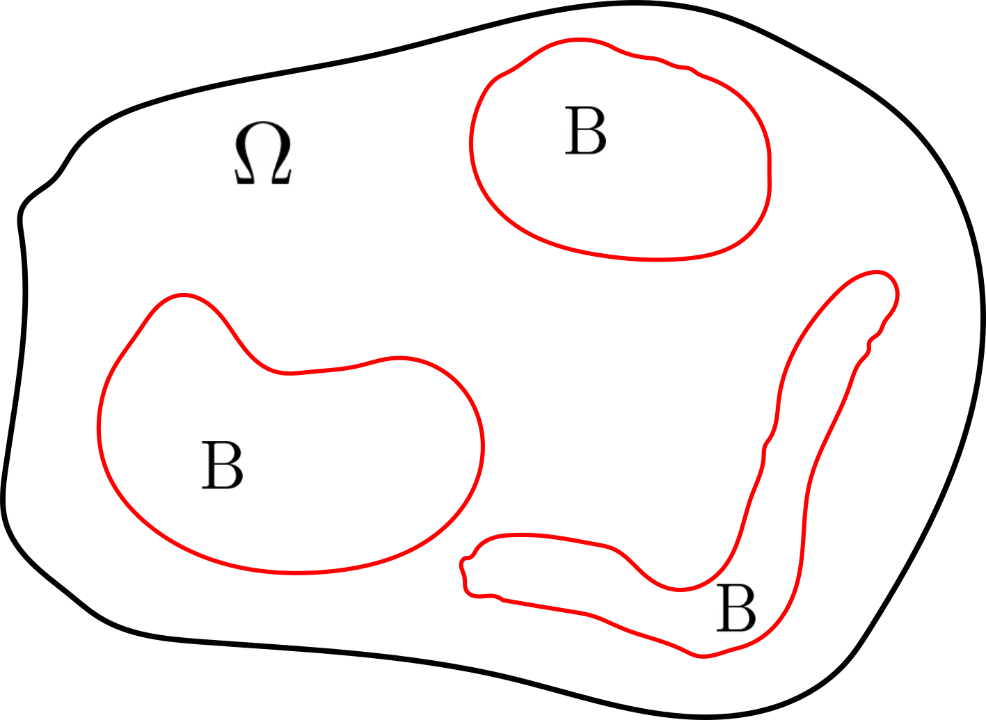
(a) Allowable

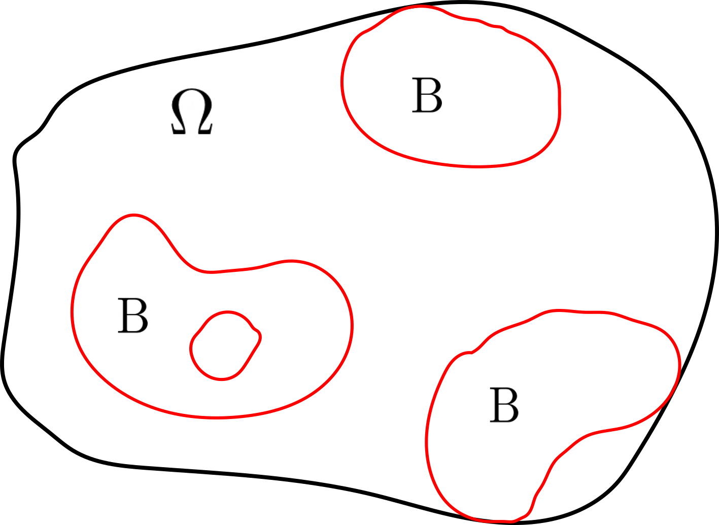
(b) Not Allowable

Figure 1: A visual depiction of allowable and not allowable configurations of the region $B$.

Assumption 2.

The function $f:(\overline{\Omega}\setminus B)\times[0,\infty)\to\mathbb{R}$ is assumed to satisfy the following conditions.

1. $f(\cdot,0)\equiv 0$, $f(\cdot,u)$ is Hölder continuous with exponent $\alpha\in(0,1)$ uniform with respect to $u$ in bounded sets;

2. $f(x,\cdot)\in C^{1}([0,\infty))$ for each $x\in\overline{\Omega}\setminus B$, $f_{u}(\cdot,0)$ is Hölder continuous with exponent $\alpha\in(0,1)$, and $f_{u}(x,0)>0$ for some $x\in\Omega\setminus\overline{B}$;

3. For each $x\in\Omega\setminus\overline{B}$, $f(x,\cdot)$ is strictly concave down.

Conditions (1)-(2) are standard regularity assumptions that ensure solutions are sufficiently smooth for our subsequent analysis. The positivity of $f_{u}(\cdot,0)$ somewhere in $\Omega\setminus\overline{B}$ is necessary to ensure that a positive steady state may exist; without this condition, the only steady state will be the trivial one. Paired with the regularity of the domains $\Omega$ and $B$, we also have regularity up to the boundary $\partial\Omega$ and up to $\partial B$ for problem (1.2). Condition (3) ensures the uniqueness of the positive steady state (whenever it exists) and that the flow induced by the dynamical system is strongly monotone. We require a strict concavity condition to obtain convergence from the time-dependent problem to the corresponding steady-state uniformly in the variable $c$. A prototypical example satisfying Assumption 2 is the heterogeneous logistic form $f(x,u)=u(m(x)-u)$ for some Hölder continuous function $m(x)$. For the remainder of the manuscript, Assumptions 1 and 2 are always assumed whenever $B$ and $f$ are involved.

In the remainder of this subsection, we introduce function spaces over the domain $\Omega\setminus\overline{B}$ and their relation to similar spaces over the entire domain $\Omega$. We introduce the space $C_{B}^{1}(\Omega)$ as

$$C_{B}^{1}(\Omega):=\left\{v\in C^{1}(\overline{\Omega}\setminus B):v|_{\partial B}=0\right\},$$

and consider $H_{B}^{1}(\Omega)$ to be the closure of the space $C_{B}^{1}(\Omega)$ with respect to the $H^{1}$-norm over $\Omega\setminus\overline{B}$. In this way, $H_{B}^{1}(\Omega)$ can be considered similar to the space $H_{0}^{1}(\Omega)$, with functions now vanishing along $\partial B$ in the trace sense. More precisely, it can be verified that

$$H_{B}^{1}(\Omega)=\left\{u\in H^{1}(\Omega\setminus\overline{B}):\textbf{T}u=0\right\},$$

where T denotes the trace operator extending the notion of restricting a function on $\Omega\setminus B$ to $\partial B$.

For any $u\in C_{B}^{1}(\Omega)$ or $H_{B}^{1}(\Omega)$, we identify it with its zero extension into $B$. If $u\in H_{B}^{1}(\Omega)$, then the resulting function belongs to $H^{1}(\Omega)$. Conversely, if $u\in H^{1}(\Omega)$ with $u=0$ a.e. in $B$, then $u|_{\Omega}\in H_{B}^{1}(\Omega)$. Therefore, we identify $H_{B}^{1}(\Omega)$ with $\left\{u\in H^{1}(\Omega):u=0\,\,\text{a.e. in}\,\,B\right\}$, and simply write

$$\begin{split}H_{B}^{1}(\Omega)=\left\{u\in H^{1}(\Omega):u=0\,\,\text{a.e. in}\,\,B\right\}.\end{split}$$

We wish to emphasize that these results rely crucially on the smoothness of $\partial B$ and the fact that $B\Subset\Omega$; for less regular $B$, these two formulations need not agree [6, 5].

Similarly, for $T>0$, we set $Q_{T}:=\Omega\times(0,T)$ and $Q_{B,T}:=(\Omega\setminus\overline{B})\times(0,T)$, and define $H_{B}^{1}(Q_{T})$ to the closure of $\left\{v\in C^{1}((\Omega\setminus B)\times[0,T]):v(\partial B\times[0,T])=0\right\}$ under the $H^{1}$-norm over $(\Omega\setminus\overline{B})\times(0,T)$. Similarly, by the regularity of the set $B$ there holds

$$H_{B}^{1}(Q_{T})=\left\{u\in H^{1}(Q_{B,T}):\textbf{T}u=0\right\}=\left\{u\in H^{1}(Q_{T}):u=0\,\,\text{a.e. in}\,\,B\times(0,T)\right\}.$$

1.3 Main results

It is well-known (see, e.g., [27, 47]) that the principal spectral theory of eigenvalue problems associated with the linearization of (1.1) and (1.2) about their respective trivial states play a crucial role in the investigation of their dynamics. We introduce them here and refer the reader to Appendix A.2 for a more general consideration of related concepts and results.

The eigenvalue problem associated with the linearization of (1.1) about the trivial state reads

$$\begin{cases}d\Delta\phi+m_{c}\phi+\mu\phi=0,&\text{in}\quad\Omega,\\ \frac{\partial\phi}{\partial\nu}=0,&\text{on}\quad\partial\Omega,\end{cases}$$ (1.3)

where $m_{c}=\mathbbm{1}_{\Omega\setminus B}f_{u}(\cdot,0)-c\mathbbm{1}_{B}$. Since $m_{c}\in L^{\infty}(\Omega)$ by Assumption 2, Proposition A.18 applies to (1.3). In the remainder of the current work, we say that a problem has a principal eigenvalue if it has a positive eigenfunction. Denote by $\mu_{1,c}$ the principal eigenvalue of (1.3), and by $\phi_{1,c}$ the associated positive eigenfunction.

The eigenvalue problem associated with the linearization of (1.2) about the trivial state reads

$$\begin{cases}d\Delta\phi+f_{u}(\cdot,0)\phi+\mu\phi=0,&\text{in}\quad\Omega\setminus\overline{B},\\ \frac{\partial\phi}{\partial\nu}=0,&\text{on}\quad\partial\Omega,\\ \phi=0,&\text{on}\quad\partial B.\end{cases}$$ (1.4)

As $f_{u}(\cdot,0)\in L^{\infty}(\Omega\setminus\overline{B})$ by Assumption 2, Proposition A.19 applies to (1.4). Denote by $\mu_{1,\infty}$ the principal eigenvalue of (1.4), and by $\phi_{1,\infty}$ the associated positive eigenfunction.

Our first result establishes the connection between the principal eigenpairs of (1.3) and (1.4) as $c\to\infty$.

Theorem 1.1.

The following hold.

1. The function $c\mapsto\mu_{1,c}$ is strictly increasing on $(0,\infty)$, and $\lim_{c\to\infty}\mu_{1,c}=\mu_{1,\infty}$.

2. $\lim_{c\to\infty}\phi_{1,c}=\phi_{1,\infty}$ in $H^{1}(\Omega)$ under the normalization $\|\phi_{1,c}\|_{L^{2}(\Omega)}=\|\phi_{1,\infty}\|_{L^{2}(\Omega\setminus\overline{B})}=1$.

When one considers $-\mu_{1,c}$ to be the average growth rate of the population [8], this result suggests the intuitive insight that degrading the habitat affects the population growth rate in a monotonic way. We are able to prove the following results.

Theorem 1.2.

Assume $\mu_{1,\infty}<0$. Then, (1.2) admits a unique positive steady state $u^{*}_{\infty}$ and (1.1) admits a unique positive steady state $u_{c}^{*}$ for all $c\gg 1$. Moreover,

$$\lim_{c\to\infty}u_{c}^{*}=u^{*}_{\infty}\quad\text{in}\quad C(\overline{\Omega}).$$

Note that $-\mu_{1,\infty}>0$ implies that the average population growth rate is positive for any level of degradation. We point out that in Theorem 1.2, the case $\mu_{1,\infty}>0$ is of little interest as $0$ is the only steady state to (1.2) and therefore also to (1.1) for all $c\gg 1$.

Theorem 1.3.

Assume that $\mu_{1,\infty}\neq 0$. Let $u_{c}$ and $u_{\infty}$ be the unique solutions to problems (1.1) and (1.2), respectively, with the initial data satisfying $0\lneq u_{c}(\cdot,0)=u_{\infty}(\cdot,0)\in C_{B}^{1}(\overline{\Omega})$ and $\operatorname*{supp}(u_{\infty}(\cdot,0))\Subset\overline{\Omega}\setminus\overline{B}$. Then,

$$\lim_{c\to\infty}u_{c}=u_{\infty}\quad\text{uniformly in}\quad\overline{\Omega}\times[0,\infty).$$

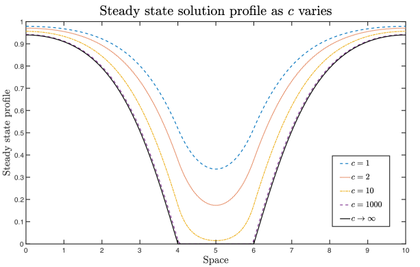
Figure 2: A simulation demonstrating Theorem 1.2 in one spatial dimension. Here, $\Omega=(0,10)$, $B=(4,6)$, $d=1$, and $f(x,u)=u(1-u)$ in $(0,4)\cup(6,10)$. The steady-state solution profile $u_{c}^{*}$ is extracted for varying levels of $c$. In this example, $\mu_{1,\infty}<0$ so that the a nontrivial steady state $u_{\infty}^{*}$ exists and there is no extinction threshold.

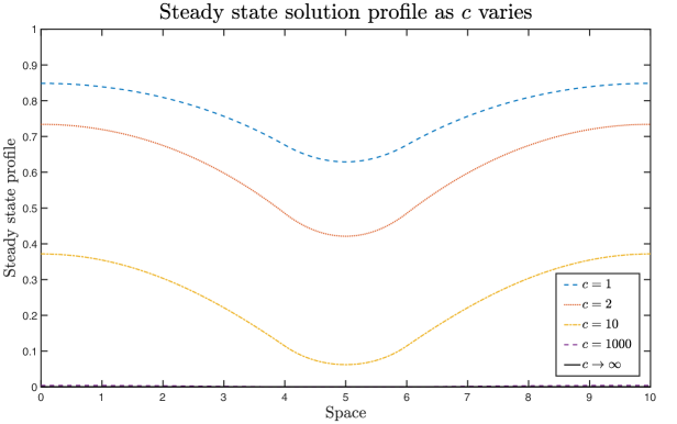
Figure 3: A numerical simulation with identical parameters as in Figure 2, except $d=6.75$. In this case, $\mu_{1,\infty}>0$ so that $u_{\infty}^{*}\equiv 0$ is the only steady state solution to the habitat destruction problem. Consequently, an extinction threshold $c_{0}\approx 1000$ exists.

Remark 1.4.

Convergence in each of these results holds in the sense that solutions to the degradation problem converge uniformly in $\overline{\Omega}\setminus B$ to the solution of the associated destruction problem while converging uniformly to zero in the set $\overline{B}$. This way, we identify the solutions to the destruction problems with their (continuous) extension by zero in the set $B$. This convention is assumed throughout the remainder of this paper.

In proving Theorem 1.3, one of the major difficulties is the uniform convergence on a large time interval $(T,\infty)$, independent of $c$. This challenge is overcome through several steps, using a uniform convergence result in an arbitrary time interval $(0,T]$, and careful use of asymptotic stability results for the degradation and destruction problems (see Theorems 3.7 and 3.9), which hold in a uniform sense with respect to parameter $c$ when $\mu_{1,\infty}\neq 0$.

We briefly discuss the restriction on the allowable initial data, as it is a technical reason. Since we are showing uniform results in the parameter $c$, we must have some control over the comparison between the initial data and a corresponding eigenfunction. For any fixed $c>0$, restriction on the initial data is unnecessary; however, in the limit, obtaining control of the eigenfunction along the boundary of the set $B$ is very difficult. Despite this technicality, the application to habitat degradation and destruction questions remains robust.

Theorems 1.2-1.3 provide a clear and direct connection between habitat degradation and destruction. Firstly, it suggests that arbitrary levels of degradation do not guarantee the displacement of local species - indeed, even in the limit as $c\to\infty$, the species may survive; of course, as the area of the degraded/destroyed region increases, the chances of survival decreases, a direct consequence of the monotonicity of the principal eigenvalue with respect to subregions of destroyed habitat (see Proposition A.17[(i)] and Proposition A.19[(iv)]). Moreover, this connection is monotone in the following sense: given solutions $u_{c}$, $c>0$ with the same initial data picking from $C^{+}(\overline{\Omega})\setminus\{0\}$, $c_{2}>c_{1}$ implies that $u_{c_{2}}<u_{c_{1}}$ in $\overline{\Omega}\times(0,\infty)$. See Lemma 3.12 for the proof. This monotone behavior provides valuable insight to empirical studies investigating differing forms of habitat loss, which occasionally yield confusing results when the direction of impact is not monotone, i.e., it is sometimes observed that habitat loss is beneficial to certain species. Our results suggest that any positive effect a local species may experience in a region of altered habitat must come from another process, such as that of fragmentation or species-species interactions, and may be influenced more directly by more complicated factors, such as an edge effect [30, 14].

As a Corollary to these analytical insights, we have necessary and sufficient conditions for the existence of an extinction threshold for problem (1.1).

Corollary 1.5.

Problem (1.1) admits an extinction threshold $c_{0}\in(0,\infty)$ if and only if $\mu_{1,\infty}>0$. Moreover, in the case of $\mu_{1,\infty}>0$, the following hold.

• $c_{0}>\frac{1}{\left|B\right|}\int_{\Omega\setminus B}f_{u}(x,0){\rm d}x$.

• Denote by $u_{c}$ the unique solution to problem (1.1) with initial data $u_{c}(\cdot,0)\in C^{+}(\overline{\Omega})\setminus\{0\}$. Then,

  $$\lim_{t\to\infty}u_{c}(\cdot,t)=\begin{cases}u_{c}^{*},&\text{if}\quad 0<c<c_{0},\\ 0,&\text{if}\quad c>c_{0}\end{cases}\quad\text{in}\quad C(\overline{\Omega}).$$

• Suppose that $u_{c}(\cdot,0)$ is independent of $c$. Then, for any $\tilde{c}>c_{0}$, there exist $r=r(\tilde{c})>0$ and $M>0$ (depending only on $\tilde{c}$ and the common initial data) such that

  $$\sup_{c\geq\tilde{c}}\left\|u_{c}(\cdot,t)\right\|_{C(\overline{\Omega})}\leq Me^{-rt},\quad\forall t\geq 0.$$

By (1), we can therefore always increase the extinction threshold $c_{0}$ by decreasing the size of the degraded region $B$, or by improving the habitat quality in the undisturbed region $\Omega\setminus B$.

1.4 Organization

We organize the remainder of the paper as follows. In Section 2, we study the connection between eigenvalue problems and prove Theorem 1.1. Section 3 is devoted to the investigation of the connection between Cauchy problems (1.1) and (1.2). In particular, we prove Theorems 1.2 and 1.3. We discuss some implications of our results and related issues in Section 4. Appendix A is included to collect some well-known results about eigenvalue problems that are used throughout the paper.

2 Connection between eigenvalue problems

In this section, we study the connection between problems (1.3) and (1.4), and prove Theorem 1.1. We then study the related sign-indefinite weight problems, providing a robust and complete picture of the connections between these two sets of eigenvalue problems. We refer the reader to Appendix A for more general consideration of eigenvalue problems with sign-indefinite weight and their connections to usual eigenvalue problems like (1.3) and (1.4).

We first prove Theorem 1.1.

Proof of Theorem 1.1.

Recall that $\mu_{1,c}$ has the variational characterization (see Proposition A.18):

$$\mu_{1,c}=\inf_{\phi\in H^{1}(\Omega)}\left\{\int_{\Omega}\left(d\left|\nabla\phi\right|^{2}-m_{c}\phi^{2}\right)\ :\ \int_{\Omega}\phi^{2}=1\right\}.$$ (2.1)

By Proposition A.18 (ii), we see that $\mu_{1,c}$ is strictly increasing in $c$. Since $\phi_{1,\infty}\in H_{B}^{1}(\Omega)$, $\phi_{1,\infty}\in H^{1}(\Omega)$ by zero extension in $B$. It follows from (2.1) and the normalization $\int_{\Omega}\phi_{1,\infty}^{2}=1$ that

$$\mu_{1,c}\leq\int_{\Omega}\left(d\left|\nabla\phi_{1,\infty}\right|^{2}-m_{c}\phi_{1,\infty}^{2}\right)=\int_{\Omega\setminus\overline{B}}\left(d\left|\nabla\phi_{1,\infty}\right|^{2}-f_{u}(\cdot,0)\phi_{1,\infty}^{2}\right)=\mu_{1,\infty},$$

where the second equality is a result of the eigen-equation satisfied by $\mu_{1,\infty}$ and $\phi_{1,\infty}$. Thus, $\mu_{1,c}$ is strictly increasing and uniformly bounded by $\mu_{1,\infty}$. Hence, $\mu_{\infty}:=\lim_{c\to\infty}\mu_{1,c}$ exists and is finite. Obviously, $\mu_{\infty}\leq\mu_{1,\infty}$.

From the eigen-equation satisfied by $\mu_{1,c}$ and $\phi_{1,c}$ (or (2.1) with the understanding that the infimum is attained at $\phi_{1,c}$),

$$d\int_{\Omega}\left|\nabla\phi_{1,c}\right|^{2} =\mu_{1,c}+\int_{\Omega}m_{c}\phi_{1,c}^{2}\leq\mu_{\infty}+\left\|f_{u}(\cdot,0)\right\|_{L^{\infty}(\Omega\setminus\overline{B})},$$

where we have thrown away the negative term and used the normalization $\int_{\Omega}\phi_{1,c}^{2}=1$. Hence, $\{\phi_{1,c}\}_{c>0}$ is bounded in $H^{1}(\Omega)$. Consequently, there exists a subsequence (still denoted by $\phi_{1,c}$) and some $\phi_{\infty}\in H^{1}(\Omega)$ such that

$$\lim_{c\to\infty}\phi_{1,c}=\phi_{\infty}\quad\text{weakly in}\,\,H^{1}(\Omega)\quad\text{and}\quad\text{strongly in}\,\,L^{2}(\Omega).$$ (2.2)

Note that

$$c\int_{B}\phi_{1,c}^{2}=\mu_{1,c}+\int_{\Omega\setminus\overline{B}}f_{u}(\cdot,0)\phi_{1,c}^{2}-d\int_{\Omega}\left|\nabla{\phi_{1,c}}\right|^{2}\leq\mu_{\infty}+\left\|f_{u}(\cdot,0)\right\|_{L^{\infty}(\Omega\setminus\overline{B})},$$

leading to $\int_{B}\phi_{1,c}^{2}\leq\frac{1}{c}\left(\mu_{\infty}+\left\|f_{u}(\cdot,0)\right\|_{L^{\infty}(\Omega\setminus\overline{B})}\right)\to 0$ as $c\to\infty$. This together with the strong convergence in (2.2) implies $\int_{B}\phi_{1,\infty}^{2}=0$. Hence, $\phi_{\infty}=0$ a.e. in $B$, and so, $\phi_{\infty}\in H_{B}^{1}(\Omega)$. Furthermore, since $\int_{\Omega}\phi_{1,c}^{2}=1$, the strong convergence in (2.2) implies that $\int_{\Omega}\phi_{\infty}^{2}=1$. Hence, $\phi_{\infty}$ is nonzero and is a valid test function in the variational characterization of $\mu_{1,\infty}$.

We now show that $\mu_{1,\infty}\leq\mu_{\infty}$. Note that $\mu_{1,\infty}$ has the variational characterization (see Proposition A.19):

$$\mu_{1,\infty}=\inf_{\phi\in H_{B}^{1}(\Omega)}\left\{\int_{\Omega\setminus\overline{B}}\left(d\left|\nabla\phi\right|^{2}-f_{u}(\cdot,0)\phi^{2}\right)\ :\ \int_{\Omega\setminus\overline{B}}\phi^{2}=1\right\}.$$

This together with the weak lower semicontinuity of the norm $\|\cdot\|_{L^{2}(\Omega)}$ and (2.2) leads to

$$\mu_{1,\infty} \leq\int_{\Omega\setminus\overline{B}}d\left|\nabla\phi_{\infty}\right|^{2}-\int_{\Omega\setminus\overline{B}}f_{u}(\cdot,0)\phi_{\infty}^{2}$$

$$=\int_{\Omega}d\left|\nabla\phi_{\infty}\right|^{2}-\int_{\Omega}m_{c}\phi_{\infty}^{2}$$

$$\leq\liminf_{c\to\infty}\int_{\Omega}d\left|\nabla\phi_{1,c}\right|^{2}-\lim_{c\to\infty}\int_{\Omega}m_{c}\phi_{1,c}^{2}=\liminf_{c\to\infty}\mu_{1,c}=\mu_{\infty}.$$

Hence,

$$\mu_{\infty}=\lim_{c\to\infty}\mu_{1,c}=\mu_{1,\infty}.$$ (2.3)

In particular, this implies that $\phi_{\infty}$ solves the same eigenvalue problem as $\phi_{1,\infty}$, and hence, $\phi_{\infty}=\phi_{1,\infty}$ by the uniqueness of the eigenfunction and the chosen normalization.

It remains to show $\lim_{c\to\infty}\nabla\phi_{1,c}=\nabla\phi_{\infty}$ in $L^{2}(\Omega)$ so that $\lim_{c\to\infty}\phi_{1,c}=\phi_{\infty}$ in $H^{1}(\Omega)$. Note that

$$d\int_{\Omega}\left(\left|\nabla\phi_{1,c}\right|^{2}-\left|\nabla\phi_{\infty}\right|^{2}\right) =\mu_{1,c}-\mu_{1,\infty}+\int_{\Omega\setminus\overline{B}}f_{u}(\cdot,0)(\phi_{1,c}^{2}-\phi_{\infty}^{2})-c\int_{B}\phi_{1,c}^{2}$$

$$\leq\mu_{1,c}-\mu_{1,\infty}+\int_{\Omega\setminus\overline{B}}f_{u}(\cdot,0)(\phi_{1,c}^{2}-\phi_{\infty}^{2}).$$

Letting $c\to\infty$ in the above inequality, we see from (2.3) and the strong convergence in (2.2) that $\limsup_{c\to\infty}\int_{\Omega}{\left|\nabla\phi_{1,c}\right|^{2}}\leq\int_{\Omega}\left|\nabla\phi_{\infty}\right|^{2}$. As $\liminf_{c\to\infty}\int_{\Omega}{\left|\nabla\phi_{1,c}\right|^{2}}\geq\int_{\Omega}\left|\nabla\phi_{\infty}\right|^{2}$ due to the weak lower semicontinuity of the norm $\|\cdot\|_{L^{2}(\Omega)}$ and the weak convergence in (2.2), we find $\lim_{c\to\infty}\int_{\Omega}{\left|\nabla\phi_{1,c}\right|^{2}}=\int_{\Omega}\left|\nabla\phi_{\infty}\right|^{2}$, which together with the weak convergence in (2.2) yields $\lim_{c\to\infty}\nabla\phi_{1,c}=\nabla\phi_{1,\infty}$ in $L^{2}(\Omega)$. ∎

In the rest of this section, we explore further the eigenvalue problems with sign-indefinite weight associated with (1.3) and (1.4), that is,

$$\begin{cases}\Delta\psi+\lambda m_{c}\psi=0,&\text{in}\quad\Omega,\\ \frac{\partial\psi}{\partial\nu}=0,&\text{on}\quad\partial\Omega,\end{cases}$$ (2.4)

and

$$\begin{cases}\Delta\psi+\lambda f_{u}(\cdot,0)\psi=0,&\text{in}\quad\Omega\setminus\overline{B},\\ \frac{\partial\psi}{\partial\nu}=0,&\text{on}\quad\partial\Omega,\\ \psi=0,&\text{on}\quad\partial B.\end{cases}$$ (2.5)

While not directly related to the results obtained for the Cauchy problems in subsequent sections, it is necessary to also establish a connection between the principal eigenvalues to problems (2.4) and (2.5) in order to completely describe the relationship to problems (1.3) and (1.4), particularly in the limiting case. We make this more precise following the statement of Theorem 2.6.

It is easy to see that Assumption 2 ensures that $m_{c}\in L^{\infty}(\Omega)$ is sign-changing and $f_{u}(\cdot,0)\in L^{\infty}(\Omega\setminus\overline{B})$ is positive on a set of positive Lebesgue measure. Thus, Propositions A.16 and A.17 apply to (2.4) and (2.5), respectively. Set $c_{*}:=\frac{1}{\left|B\right|}\int_{\Omega\setminus B}f_{u}(\cdot,0)$. It is elementary to see that $\int_{\Omega}m_{c}<0$ for all $c>c_{*}$. For each $c>c_{*}$, we denote by $\lambda_{1,c}$ the unique nonzero principal eigenvalue of (2.4), and by $\psi_{1,c}$ the associated positive eigenfunction. Denote by $\lambda_{1,\infty}$ the unique positive principal eigenvalue of (2.5), and by $\psi_{1,\infty}$ the associated positive eigenfunction.

We prove the following result, connecting the principal eigenpairs of (2.4) and (2.5) as $c\to\infty$.

Theorem 2.6.

The following hold.

1. The function $c\mapsto\lambda_{1,c}$ is strictly increasing on $(c_{*},\infty)$, and $\lim_{c\to\infty}\lambda_{1,c}=\lambda_{1,\infty}$.

2. $\lim_{c\to\infty}\psi_{1,c}=\psi_{1,\infty}$ in $H^{1}(\Omega)$ under the normalization $\int_{\Omega}m_{c}\psi_{1,c}^{2}=\int_{\Omega\setminus B}f_{u}(\cdot,0)\psi_{1,\infty}^{2}=1$.

We can now make clear the important connection such a result endows. Proposition A.18 (iii) provides a way of characterizing the sign of $\mu_{1,c}$ based on $\lambda_{1,c}$ and its relation to the size of the diffusion coefficient $d$. Similarly, Proposition A.19 (iv) gives the same result for $\mu_{1,\infty}$, whose sign is characterized by a relation between $\lambda_{1,\infty}$ and the diffusion coefficient. Given that $\lim_{c\to\infty}\mu_{1,c}=\mu_{1,\infty}$, it is expected that the quantity used to determine the sign of these eigenvalues should remain consistent. Theorem 2.6 confirms this is indeed the case, completing the analytical connection between these four problems. However, the biological insights gained by confirming this connection are also interesting. Based on Propositions A.18 and A.19, as is well known, a smaller diffusion rate is favorable for a population’s persistence in this model framework. How low the diffusion rate must be to ensure persistence (or extinction, in the case of undesirable pest populations, for example) depends precisely on the size of the principal eigenvalues. With the convergence result established in Theorem 2.6, under increasing habitat degradation, the limiting case acts as a “worst case scenario”, providing a necessary and sufficient condition for the survival of species for any $c\in(c_{*},\infty)$. Alternatively, it provides insights into whether extinction is a possibility: if $d<\lambda_{1,\infty}^{-1}$, extinction in the degradation case is impossible; otherwise, there will be $c$ large enough to ensure the eradication of the population.

Proof of Theorem 2.6.

Since the proof is almost identical to the proof of Theorem 1.1, we outline only the key steps. First, it is easy to deduce that $\lambda_{1,c}$ is strictly increasing and bounded above by $\lambda_{1,\infty}$. As a result, its limit exists and is given by the supremum, denoted by $\lambda_{\infty}$. Then, we find that $\psi_{1,c}$ is uniformly bounded in $H^{1}(\Omega)$ and thus has a convergent subsequence, weakly in $H^{1}(\Omega)$ and strongly in $L^{2}(\Omega)$. Denote this by $\psi_{\infty}$. Furthermore, $\psi_{1,c}\to 0$ a.e. in $B$, and so the candidate function $\psi_{\infty}\in H_{B}^{1}(\Omega)$ as argued previously. One can show show that $\lambda_{1,\infty}\leq\lambda_{\infty}$ by the weak lower semicontinuity of the norm. This implies that $\nabla\psi_{1,c}\to\nabla\psi_{\infty}$ in norm, and hence the convergence is in fact strong. Uniqueness of the eigenfunction allows one to conclude that $\psi_{\infty}=\psi_{1,\infty}$. ∎

3 Connection between Cauchy problems

The purpose of this section is to establish a robust connection between the degradation problem (1.1) and the destruction problem (1.2) as given in Theorems 1.2 and 1.3.

3.1 Global dynamics of degradation and destruction problems

We first present results about the global well-posedness of the problems (1.1) and (1.2). For (1.2), the existence and uniqueness of a global classical solution

$$\begin{split}&u_{\infty}\in C^{2+\alpha,1+\alpha/2}((\Omega\setminus\overline{B})\times(0,\infty))\cap C^{+}((\overline{\Omega}\setminus B)\times[0,\infty))\\ &\text{with}\,\,u_{\infty}(0,\cdot)\in H_{B}^{1}(\Omega)\cap C^{+}(\overline{\Omega}\setminus{B})\end{split}$$ (3.1)

follows from the classical local well-posedness theory (see e.g. [39, Chapter 2]) and the comparison principle.

For (1.1), the existence and uniqueness of a global strong solution

$$\begin{split}&u_{c}\in C^{\alpha}([0,\infty);C^{+}(\overline{\Omega}))\cap C^{1}((0,\infty);C^{+}(\overline{\Omega}))\\ &\text{with}\,\,u_{c}(0,\cdot)\in C^{+}(\overline{\Omega})\end{split}$$ (3.2)

follows from the proof of [43, Theorem 2.1] (with proper modifications to approximate $\mathbbm{1}_{\Omega\setminus B}f(x,u)$) and the comparison principle. While the solution $u_{c}$ is not twice continuously differentiable in space due to the discontinuity in the right hand side of (1.1), $u_{c}\in C^{1+\alpha,(1+\alpha)/2}(Q_{T})$ for any $\alpha\in(0,1)$ and any $T>0$ by the Sobolev embedding. It is important to point out that these regularity results hold for each $c>0$ fixed, but do not a priori hold independent of $c$.

In what follows, $u_{c}$ and $u_{\infty}$ are respectively understood in the sense of (3.2) and (3.1) unless otherwise specified.

The global dynamics of the (fixed) habitat degradation problem (1.1) is given in the following.

Theorem 3.7.

The following hold for each $c\in(0,\infty)$.

1. If $\mu_{1,c}<0$, then (1.1) admits a unique positive steady state $u_{c}^{*}\in W^{1,p}(\Omega)$ for any $p\geq 1$, and $u_{c}(\cdot,t)\to u_{c}^{*}$ in $C(\overline{\Omega})$ as $t\to\infty$ whenever $u_{c}(0,\cdot)\not\equiv 0$;

2. If $\mu_{1,c}\geq 0$, then $0$ is the only steady-state solution to (1.1) and $u_{c}(\cdot,t)\to 0$ in $C(\overline{\Omega})$ as $t\to\infty$.

Moreover,

• if $\mu_{1,\infty}\leq 0$, then $\rm(i)$ holds for any $c\in(0,\infty)$;

• if $\mu_{1,\infty}>0$, then there exists $c^{*}>0$ such that $\rm(i)$ holds for all $c\in(0,c^{*})$ and $\rm(ii)$ holds for all $c\in(c^{*},\infty)$.

Proof.

This result follows from essentially from classical results, see e.g. [37, Ch. 4, Theorem 4.1], alongside some of the arguments made in [43] since the function $\mathbbm{1}_{\Omega\setminus B}f(x,u)-c\mathbbm{1}_{B}u$ may be discontinuous along $\partial B$. More precisely, a strong monotonicity result holds for problem (1.1), and the uniqueness of the positive steady state follows from the concavity of the function $f(x,u)-c\mathbbm{1}_{B}u$ (see Proposition 2.2 and Theorem 2.1 in [43]; the weaker condition strong subhomogeneity is sufficient). The result then follows from the theory of monotone flows. The “Moreover” part follows directly from Theorem 1.1(1). ∎

Remark 3.8.

Whenever it exists, the unique quantity $c^{*}$ is exactly the extinction threshold given in Corollary 1.5. This value is the precise point at which any further habitat degradation (for a fixed configuration $B$) results in deterministic extinction. Figures 2-3 provide a simulation of two cases for which an extinction threshold exists and does not exist.

The global dynamics of the destruction problem (1.2) are summarized in the next result.

Theorem 3.9.

Assume $0\lneq u_{\infty}(0,\cdot)\in C_{B}^{1}(\overline{\Omega})$. The following hold.

1. If $\mu_{1,\infty}<0$, then (1.2) admits a unique positive steady state $u^{*}_{\infty}\in C^{2+\alpha}(\Omega\setminus\overline{B})\cap C(\overline{\Omega}\setminus B)$, and $u_{\infty}\to u^{*}_{\infty}$ in $C(\overline{\Omega}\setminus B)$ as $t\to\infty$;

2. If $\mu_{1,\infty}\geq 0$, then $0$ is the only steady state to (1.2), and $u_{\infty}\to 0$ in $C(\overline{\Omega}\setminus B)$ as $t\to\infty$.

Proof.

This result follows from similar arguments made in the proof of Theorem 3.7, however there are some technical issues to address due to the Dirichlet boundary condition along the boundary $\partial B$. To address this, we set $X:=C_{B}^{1}(\overline{\Omega})$ and recall the strong partial order on $X$ generated by the cone $X^{+}=\left\{v\in X:v\geq 0\right\}$ with interior

$$X^{++}=\left\{v\in X:v>0\text{ in }\overline{\Omega}\setminus\overline{B}\text{ and }\frac{\partial v}{\partial\nu}<0\text{ on }\partial B\right\}.$$

The global existence, uniqueness and regularity of solutions to (1.2) with initial data in $X^{+}$, paired with the comparison principle, ensure that (1.2) generates a strongly monotone flow on $X^{+}$.

When $\mu_{1,\infty}<0$, the existence of a positive steady state $u^{*}\in X^{++}$ follows from a sub/super solution argument, where any sufficiently large constant acts as a super solution due to Assumption 2 (3), and $w=\varepsilon\tilde{\psi}_{1}$ acts as a sub solution since we may choose $\varepsilon$ sufficiently small but positive so that $f_{u}(\cdot,0)-\frac{f(\cdot,w)}{w}\leq-\mu_{1}(\infty)$, again by Assumption 2 (3). Furthermore, the concavity ensures that the steady state is unique (subhomogeneity is sufficient, see [47, Ch. 2.3]). Since problem (1.2) generates a strongly monotone flow in $X^{+}$, we then conclude that $u^{*}$ is globally attractive for any initial data $u_{0}\in X^{+}\setminus\{0\}$.

When $\mu_{1,\infty}\leq 0$, $0$ is the only steady state solving problem (1.2) since $w=\varepsilon\tilde{\psi}_{1}$ is a (strict) super solution for all $\varepsilon>0$ by Assumption 2 (3), and $0$ is globally attractive. ∎

3.2 From habitat degradation to habitat destruction: steady states

This subsection is devoted to the convergence between the steady states $u_{c}^{*}$ and $u^{*}_{\infty}$ as $c\to\infty$ as stated in Theorem 1.2. We need the following lemma.

Lemma 3.10.

Assume $\mu_{1,\infty}<0$. Then, for any $0<\underline{c}<\overline{c}$, there holds $u_{\infty}^{*}\leq u_{\overline{c}}^{*}<u_{\underline{c}}^{*}$ in $\overline{\Omega}$.

Proof.

Since $\mu_{1,\infty}<0$, $u_{c}^{*}$ exists for all $c>0$. Then, it is easy to see that $u_{\overline{c}}^{*}\leq u_{\underline{c}}^{*}$ by the concavity of $f(x,\cdot)$ and the strong maximum principle for strong solutions, see the proof of e.g. [43, Proposition 2.2]. The the strong maximum principle and Hopf’s lemma implies that either $u_{\overline{c}}^{*}<u_{\underline{c}}^{*}$ or $u_{\overline{c}}^{*}\equiv u_{\underline{c}}^{*}$ in $\overline{\Omega}$. By the uniqueness of the steady state solution, the second cannot hold, and the strict inequality follows.

Let $c>0$. Note that both $u_{c}^{*}$ and $u_{\infty}^{*}$ satisfy

$$\begin{cases}0=d\Delta u+f(x,u),&\text{in}\quad\Omega\setminus\overline{B},\\ \frac{\partial u}{\partial\nu}=0,&\text{on}\quad\partial\Omega.\end{cases}$$

As $u_{\infty}^{*}=0<u_{c}^{*}$ on $\partial B$, we apply the comparison principle to conclude $u_{\infty}^{*}\leq u_{c}^{*}$ in $\overline{\Omega}\setminus B$. Since $u_{\infty}^{*}$ is identified with its extension by zero in $B$, we automatically have that $u_{\infty}^{*}<u_{c}^{*}$ in $\overline{B}$ by the positivity of $u_{c}^{*}$. Hence, $u_{\infty}^{*}\leq u_{c}^{*}$ in $\overline{\Omega}$. ∎

We now establish Theorem 1.2. Its proof is instructive for the more difficult parabolic analog (i.e. Theorem 1.3) as we require fewer estimates to conclude our desired result.

Proof of Theorem 1.2.

The existence and uniqueness of positive steady states follow from Theorems 3.7 and 3.9. It remains to show the convergence result.

Lemma 3.10 asserts that $\{u_{c}^{*}\}_{c\gg 1}$ is a decreasing sequence of functions bounded below by $u_{\infty}^{*}$. Hence, the pointwise limit $u^{*}:=\lim_{c\to\infty}u_{c}^{*}$ exists in $\overline{\Omega}$ and is nontrivial. This is our candidate solution to the limiting problem.

Multiplying the equation satisfied by the steady state $u_{c}^{*}$ by itself, integrating over $\Omega$ and integrating by parts, we obtain

$$d\int_{\Omega}\left|\nabla u_{c}^{*}\right|^{2}=\int_{\Omega\setminus B}f(\cdot,u_{c}^{*})u_{c}^{*}-c\int_{B}(u_{c}^{*})^{2}\leq\left\|f_{u}(\cdot,0)\right\|_{L^{\infty}(\Omega\setminus\overline{B})}\left\|u_{c}^{*}\right\|_{L^{2}(\Omega)}^{2},$$ (3.3)

where used Assumption 2 (3) in the inequality. Hence, $\{u_{c}^{*}\}_{c\gg 1}$ is bounded in $H^{1}(\Omega)$. Consequently, there exists a subsequence, still denoted by $u_{c}^{*}$, such that

$$\lim_{c\to\infty}u_{c}^{*}=u^{*}\quad\text{strongly in}\,\,L^{2}(\Omega)\quad\text{and}\quad\text{weakly in}\,\,H^{1}(\Omega).$$ (3.4)

In particular, for any $\phi\in H_{B}^{1}(\Omega)$ (considered as an element in $H^{1}(\Omega)$ after zero extension in $B$), we have $-c\int_{B}u_{c}^{*}\phi=0$ for all $c\gg 1$, and

$$\lim_{c\to\infty}d\int_{\Omega}\nabla u_{c}^{*}\cdot\nabla\phi=d\int_{\Omega}\nabla u^{*}\cdot\nabla\phi,\quad\lim_{c\to\infty}\int_{\Omega}f(\cdot,u_{c}^{*})\phi=\int_{\Omega}f(\cdot,u^{*})\phi.$$

Therefore, $u^{*}$ satisfies $-d\Delta u^{*}=f(x,u^{*})$ in $\Omega\setminus\overline{B}$ in the weak sense.

We now show that $u^{*}\in H_{B}^{1}(\Omega)$. We see from the equality in (3.3) that

$$c\int_{B}(u_{c}^{*})^{2} \leq\left\|f_{u}(\cdot,0)\right\|_{L^{\infty}(\Omega\setminus\overline{B})}\int_{\Omega}(u_{c}^{*})^{2}.$$

As $\sup_{c\gg 1}\int_{\Omega}(u_{c}^{*})^{2}<\infty$, we arrive at $\lim_{c\to\infty}\int_{B}(u_{c}^{*})^{2}=0$. It then follows from the convergence in (3.4) or the monotone convergence theorem that $\int_{B}(u^{*})^{2}=0$, and hence, $u^{*}=0$ a.e. in $B$. In particular, $u^{*}\in H_{B}^{1}(\Omega)$.

Combining these results, we conclude from the elliptic regularity theory that $u^{*}$ is a steady state to (1.2), and therefore, $u^{*}=u_{\infty}^{*}$ by the uniqueness of positive steady states. As $u^{*}\in C(\overline{\Omega})$, we conclude the result from Dini’s theorem. ∎

Remark 3.11.

We cannot expect a stronger notion of convergence over the entire domain $\Omega$ in a classical sense than what was shown above. Informally, this can be made intuitive if one considers the fact that $\frac{\partial u^{*}_{\infty}}{\partial\nu}$ is negative along $\partial B$ while $u^{*}_{\infty}$ is identically zero inside of $B$. Hence, we expect the classical derivative of $u^{*}_{\infty}$ to be discontinuous along $\partial B$. However, stronger notions of convergence are readily established away from the boundary of $B$ through the usual arguments.

3.3 From habitat degradation to habitat destruction: general solutions

This subsection is devoted to the proof of Theorem 1.3. We prove several lemmas before doing so. The following addresses the monotonicity of solutions in $c$.

Lemma 3.12.

Assume $0<\underline{c}<\overline{c}$. If $u_{\underline{c}}(\cdot,0)=u_{\overline{c}}(\cdot,0)\in C^{+}(\overline{\Omega})\setminus\{0\}$, then $u_{\underline{c}}>u_{\overline{c}}>0$ in $\overline{\Omega}\times(0,\infty)$.

Proof.

Set $w:=u_{\overline{c}}-u_{\underline{c}}$ and $w^{+}:=\max\{0,w\}$. Note that $u_{\overline{c}}$ and $u_{\underline{c}}$ are bounded. This together with the regularity assumption on $f$ implies the existence of some $K>0$ such that

$$\frac{1}{2}\frac{d}{dt}\int_{\Omega}(w^{+})^{2} =-d\int_{\Omega}\left|\nabla w^{+}\right|^{2}+\int_{\Omega}w^{+}(f(\cdot,u_{\overline{c}})-f(\cdot,u_{\underline{c}}))\leq K\int_{\Omega}(w^{+})^{2}.$$

Grönwall’s inequality implies that $w^{+}=0$ a.e. in $Q_{T}$ and hence $u_{\overline{c}}\leq u_{\underline{c}}$ holds in all of $Q_{T}$ by the smoothness of the solutions. Then, since $u_{c}\in C^{1}((0,\infty);C^{+}(\overline{\Omega}))$, the strong maximum principle for strong solutions applies, see e.g. [1]. Indeed, if there exists a point $(x_{0},t_{0})\in Q_{T}$ such that $w=0$, it follows that $w\equiv 0$ in $\Omega$ for all $t\in(0,t_{0})$, a contradiction to the uniqueness of solutions. Finally, if there exists a point $x_{0}\in\partial\Omega$ such that $w(x_{0},t_{0})=0$ for some $t_{0}>0$, Hopf’s lemma implies that $\frac{\partial w}{\partial\nu}(x_{0},t_{0})>0$, a contradiction to the homogeneous Neumann boundary condition satisfied by $w$ along $\partial\Omega$. Hence, $w<0\Rightarrow u_{\overline{c}}<u_{\underline{c}}$ in $\overline{\Omega}\times(0,\infty)$. The conclusion $u_{\overline{c}}>0$ in $\overline{\Omega}\times(0,\infty)$ follows from similar arguments. ∎

As an immediate consequence of Theorem 3.7 and Lemma 3.12, we have the following result.

Corollary 3.13.

Suppose $\mu_{1,\infty}>0$. Then, for any initial data $u_{c}(0,\cdot)\in C^{+}(\Omega)\setminus\{0\}$ independent of $c\gg 1$, there holds

$$\lim_{t\to\infty}\sup_{c\gg 1}\left\|u_{c}(\cdot,t)\right\|_{C(\overline{\Omega})}=0.$$

In fact, for any $\tilde{c}\in(c^{*},\infty)$ there exist $r=r(\tilde{c})>0$ and $M>0$ (depending only on $\tilde{c}$ and the common initial data) such that

$$\sup_{c\geq\tilde{c}}\left\|u_{c}(\cdot,t)\right\|_{C(\overline{\Omega})}\leq Me^{-rt},\quad\forall\,t\geq 0.$$

Proof.

Let $c^{*}$ be as in Theorem 3.7. Then, $\mu_{1,c}>0$ for all $c>c^{*}$. Fix $\tilde{c}>c^{*}$ and set $W:=Me^{-\mu_{1,\tilde{c}}t}\phi_{1,\tilde{c}}$, where $\phi_{1,\tilde{c}}$ is the positive eigenfunction to problem (1.3) for $m_{\tilde{c}}$. It is easy to see that $W$ is a super solution to $u_{\tilde{c}}$ whenever $M$ is chosen large enough that $u_{\tilde{c}}(\cdot,0)\leq M\phi_{1,\tilde{c}}$. One immediately has that $\lim_{t\to\infty}\left\|u_{\tilde{c}}(\cdot,t)\right\|_{C(\overline{\Omega})}\leq M\max_{\Omega}\phi_{\tilde{c}}\lim_{t\to\infty}e^{-\mu_{1,\tilde{c}}t}=0$. The result then follows from Lemma 3.12. ∎

The next result addresses the uniform convergence over finite time intervals.

Lemma 3.14.

If $u_{c}(\cdot,0)=u_{\infty}(\cdot,0)\in H_{B}^{1}(\Omega)\cap C^{+}(\overline{\Omega})$ for all $c\gg 1$ and $\operatorname*{supp}(u_{\infty}(\cdot,0))\Subset\overline{\Omega}\setminus\overline{B}$, then for each $T>0$,

$$\lim_{c\to\infty}u_{c}=u_{\infty}\,\,\text{uniformly in}\,\,\overline{\Omega}\times[0,T].$$

Proof.

Fix $T>0$ and denote by $u_{0}$ the common initial data. The proof is done in four steps.

Step 1

We show the existence of some constant $M=M(T)>0$ such that

$$\iint_{Q_{T}}\left(u_{c}^{2}+\left|\nabla u_{c}\right|^{2}+\left|\frac{\partial u_{c}}{\partial t}\right|^{2}\right)\leq M,\quad\forall c\gg 1.$$ (3.5)

Due to the lack of smoothness of the solution $u_{c}$, we first mollify the indicator functions on the right hand side of (1.1) so that the approximate solution belongs to $H^{1}(Q_{T})$. To this end, we set $\varepsilon_{0}:=\frac{1}{2}\text{dist}(\partial\Omega,\partial B)$ and define for each $\varepsilon\in(0,\varepsilon_{0})$ the sets:

$$B^{\varepsilon}=\left\{x\in\overline{\Omega}:\text{dist}(x,B)<\varepsilon\right\},\quad B_{\varepsilon}=\left\{x\in B:\text{dist}(x,\partial B)>\varepsilon\right\}.$$

Note that $B_{\varepsilon}\Subset B\Subset B^{\varepsilon}\Subset\Omega$. We regularize $\mathbbm{1}_{\Omega\setminus B}$ such that

$$\mathbbm{1}_{\Omega\setminus B}^{\varepsilon}=1\text{ in }\Omega\setminus B^{\varepsilon},\quad\mathbbm{1}_{\Omega\setminus B}^{\varepsilon}=0\text{ in }B,\quad 0\leq\mathbbm{1}_{\Omega\setminus B}^{\varepsilon}\leq 1\text{ in }B^{\varepsilon}\setminus B\quad\text{and}\quad\lim_{\varepsilon\to 0}\mathbbm{1}_{\Omega\setminus B}^{\varepsilon}=\mathbbm{1}_{\Omega\setminus B}\text{ in }L^{2}(\Omega).$$

Similarly, we regularize $\mathbbm{1}_{B}$ such that

$$\mathbbm{1}_{B}^{\varepsilon}=1\text{ in }B_{\varepsilon},\quad\mathbbm{1}_{B}^{\varepsilon}=0\text{ in }\Omega\setminus B,\quad 0\leq\mathbbm{1}_{B}^{\varepsilon}\leq 1\text{ in }B\setminus B_{\varepsilon}\quad\text{and}\quad\lim_{\varepsilon\to 0}\mathbbm{1}_{B}^{\varepsilon}=\mathbbm{1}_{B}\text{ in }L^{2}(\Omega).$$

Consider (1.1) with $\mathbbm{1}_{\Omega\setminus B}$ and $\mathbbm{1}_{B}$ replaced by $\mathbbm{1}_{\Omega\setminus B}^{\varepsilon}$ and $\mathbbm{1}_{B}^{\varepsilon}$, respectively, that is

$$\begin{cases}u_{t}=d\Delta u+\mathbbm{1}_{\Omega\setminus B}^{\varepsilon}f(x,u)-c\mathbbm{1}_{B}^{\varepsilon}u,&\text{in}\quad\Omega\times(0,\infty),\\ \frac{\partial u}{\partial\nu}=0,&\text{on}\quad\partial\Omega\times(0,\infty).\end{cases}$$ (3.6)

Denote by $u_{c}^{\varepsilon}$ the unique solution of (3.6) satisfying the initial data $u_{c}^{\varepsilon}(\cdot,0)=u_{0}$. Note that the standard $L^{2}$-theory of parabolic equations ensures that

$$\lim_{\varepsilon\to 0}u_{c}^{\varepsilon}=u_{c}\quad\text{in}\quad W^{2,1}_{2}(Q_{T}),$$ (3.7)

and the standard regularity theory ensures that $\frac{\partial u^{\varepsilon}_{c}}{\partial t}\in H^{1}(Q_{T})$.

We establish some uniform-in-$\varepsilon$ estimates of $u_{c}^{\varepsilon}$. First, we differentiate $\left\|u_{c}^{\varepsilon}(\cdot,t)\right\|_{L^{2}(\Omega)}^{2}$ with respect to time and integrate by parts to obtain:

$$\frac{d}{dt}\left\|u_{c}^{\varepsilon}(\cdot,t)\right\|_{L^{2}(\Omega)}^{2} =2\int_{\Omega}u_{c}^{\varepsilon}\left(d\Delta u_{c}^{\varepsilon}+\mathbbm{1}_{G\setminus B}^{\varepsilon}f(\cdot,u_{c}^{\varepsilon})-c\mathbbm{1}_{B}^{\varepsilon}\right)$$

$$\leq 2\int_{\Omega}\left|f(\cdot,u_{c}^{\varepsilon})u_{c}^{\varepsilon}\right|\leq 2\left\|f_{u}(\cdot,0)\right\|_{L^{\infty}(\Omega\setminus\overline{B})}\int_{\Omega}(u_{c}^{\varepsilon})^{2}.$$

Grönwall’s inequality implies that $\left\|u_{c}^{\varepsilon}(\cdot,t)\right\|_{L^{2}(\Omega)}^{2}\leq e^{M_{0}T}+\left\|u_{0}\right\|_{L^{2}(\Omega)}^{2}$, where $M_{0}:=2\left\|f_{u}(\cdot,0)\right\|_{L^{\infty}(\Omega\setminus B)}$. Integrating with respect to time yields

$$\left\|u_{c}^{\varepsilon}\right\|_{L^{2}(Q_{T})}^{2} \leq T(e^{M_{0}T}+\left\|u_{0}\right\|_{L^{2}(\Omega)}^{2}).$$ (3.8)

We now estimate higher order terms. Clearly, $u_{c}^{\varepsilon}$ satisfies

$$\iint_{Q_{T}}\left(\frac{\partial u_{c}^{\varepsilon}}{\partial t}v+d\nabla u_{c}^{\varepsilon}\cdot\nabla v\right)=\iint_{Q_{T}}\left(\mathbbm{1}_{\Omega\setminus B}^{\varepsilon}f(\cdot,u_{c}^{\varepsilon})-c\mathbbm{1}_{B}^{\varepsilon}u_{c}^{\varepsilon}\right)v,\quad\forall v\in H^{1}(Q_{T}).$$ (3.9)

Setting $v=u_{c}^{\varepsilon}$ in (3.9) we have

$$\int_{0}^{T}\frac{d}{dt}\left\|u_{c}^{\varepsilon}(\cdot,t)\right\|_{L^{2}(\Omega)}^{2}+d\left\|\nabla u_{c}^{\varepsilon}\right\|_{L^{2}(Q_{T})}^{2} =\iint_{Q_{B,T}}f(\cdot,u_{c}^{\varepsilon})u_{c}^{\varepsilon}-c\iint_{B\times(0,T)}(u_{c}^{\varepsilon})^{2}$$

$$\leq\left\|f_{u}(\cdot,0)\right\|_{L^{\infty}(\Omega\setminus\overline{B})}\left\|u_{c}^{\varepsilon}\right\|_{L^{2}(Q_{T})}^{2}.$$

Note that $\sup_{\varepsilon\in(0,\varepsilon_{0})}\sup_{c\gg 1}\left\|u_{c}^{\varepsilon}\right\|_{L^{2}(Q_{T})}<\infty$ by (3.8). Setting

$$M_{1}=M_{1}(T):=\left\|f_{u}(\cdot,0)\right\|_{L^{\infty}(\Omega\setminus\overline{B})}\sup_{\varepsilon\in(0,\varepsilon_{0})}\sup_{c\gg 1}\left\|u_{c}^{\varepsilon}\right\|^{2}_{L^{2}(Q_{T})}+\left\|u_{0}\right\|_{L^{2}(\Omega)}^{2},$$

we find the uniform bounds

$$\sup_{0\leq t\leq T}\left\|u_{c}^{\varepsilon}(\cdot,t)\right\|_{L^{2}(\Omega)}^{2}\leq M_{1},\quad\left\|\nabla u_{c}^{\varepsilon}\right\|_{L^{2}(Q_{T})}^{2}\leq\frac{M_{1}}{d},\quad\forall c\gg 1\,\,\text{and}\,\,\varepsilon\in(0,\varepsilon_{0}),$$ (3.10)

We now obtain estimates on $\frac{\partial u_{c}^{\varepsilon}}{\partial t}$. Setting $v=\frac{\partial u_{c}^{\varepsilon}}{\partial t}$ in (3.9), valid due to the mollification procedure, we deduce

$$\iint_{Q_{T}}\left|\frac{\partial u_{c}^{\varepsilon}}{\partial t}\right|^{2} =-\frac{d}{2}\iint_{Q_{T}}\frac{\partial}{\partial t}\left|\nabla u_{c}^{\varepsilon}\right|^{2}+\iint_{Q_{T}}\mathbbm{1}_{\Omega\setminus B}^{\varepsilon}f(\cdot,u_{c}^{\varepsilon})\frac{\partial u_{c}^{\varepsilon}}{\partial t}-\frac{c}{2}\iint_{Q_{T}}\mathbbm{1}_{B}^{\varepsilon}\frac{\partial}{\partial t}(u_{c}^{\varepsilon})^{2}$$

$$\leq-\frac{d}{2}\left(\left\|\nabla u_{c}^{\varepsilon}(\cdot,T)\right\|^{2}_{L^{2}(\Omega)}-\left\|\nabla u_{0}\right\|^{2}_{L^{2}(\Omega)}\right)+\frac{1}{2}\iint_{Q_{T}}\left|\frac{\partial u_{c}^{\varepsilon}}{\partial t}\right|^{2}+\frac{1}{2}\left\|f(\cdot,u_{c}^{\varepsilon})\right\|_{L^{2}(Q_{B,T})}^{2}$$

$$\quad-\frac{c}{2}\int_{B}\mathbbm{1}_{B}^{\varepsilon}\left((u_{c}^{\varepsilon})^{2}(\cdot,T)-u_{0}^{2}\right)$$

$$\leq\frac{d}{2}\left\|\nabla u_{0}\right\|^{2}_{L^{2}(\Omega)}+\frac{1}{2}\iint_{Q_{T}}\left|\frac{\partial u_{c}^{\varepsilon}}{\partial t}\right|^{2}+\frac{1}{2}\left\|f_{u}(\cdot,0)\right\|^{2}_{L^{\infty}(\Omega\setminus\overline{B})}\left\|u_{c}^{\varepsilon}\right\|^{2}_{L^{2}(Q_{T})},$$

where we have applied Young’s inequality, thrown away the negative terms, used the fact that $u_{0}\equiv 0$ in $B$. Setting

$$M_{2}=M_{2}(T):=d\left\|\nabla u_{0}\right\|^{2}_{L^{2}(\Omega)}+\left\|f_{u}(\cdot,0)\right\|^{2}_{L^{\infty}(\Omega\setminus\overline{B})}\sup_{\varepsilon\in(0,\varepsilon_{0})}\sup_{c\gg 1}\left\|u_{c}^{\varepsilon}\right\|^{2}_{L^{2}(Q_{T})},$$

we find

$$\iint_{Q_{T}}\left|\frac{\partial u_{c}^{\varepsilon}}{\partial t}\right|^{2}\leq M_{2},\quad\forall c\gg 1\,\,\text{and}\,\,\varepsilon\in(0,\varepsilon_{0}).$$ (3.11)

Passing to the limit $\varepsilon\to 0$ in (3.10) and (3.11), we conclude (3.5) from (3.7).

Step 2

By (3.5), there is a subsequence, still denoted by $u_{c}$, and a function $U\in H^{1}(Q_{T})$ such that

$$\begin{split}&\lim_{c\to\infty}u_{c}=U\quad\text{in}\quad L^{2}(Q_{T}),\\ &\lim_{c\to\infty}\frac{\partial u_{c}}{\partial t}=\frac{\partial U}{\partial t}\quad\text{weakly in}\quad L^{2}(Q_{T}),\\ &\lim_{c\to\infty}\nabla u_{c}=\nabla U\quad\text{weakly in}\quad L^{2}(Q_{T}).\end{split}$$ (3.12)

Note that in light of Lemma 3.12, $U$ must be the pointwise and monotone limit of $u_{c}$ as $c\to\infty$. We show $U=0$ a.e. in $B\times(0,T)$ so that $U\in H_{B}^{1}(Q_{T})$.

Recall that $\phi_{1,c}$ is a positive eigenfunction of (1.3) associated with the principal eigenvalue $\mu_{1,c}$. The normalization $\|\phi_{1,c}\|_{L^{2}(\Omega)}=1$ is fixed. Set $w_{c}:=Me^{-\mu_{1,c}t}\phi_{1,c}$ for some $M>0$ to be determined. Direct computations yield

$$(w_{c})_{t}-d\Delta w_{c}=(\mathbbm{1}_{\Omega\setminus B}f_{u}(\cdot,0)-c\mathbbm{1}_{B})w_{c}\geq\mathbbm{1}_{\Omega\setminus B}f(\cdot,w_{c})-c\mathbbm{1}_{B}w_{c},$$

where we used in the inequality the fact that $f(\cdot,u)\leq f^{\prime}(\cdot,0)u$ for any $u\geq 0$ due to Assumption 2 (3). Obviously, $\frac{\partial w_{c}}{\partial\nu}=0$ on $\partial\Omega$.

Theorem 1.1 (2) says $\lim_{c\to\infty}\phi_{1,c}=\phi_{1,\infty}$ in $H^{1}(\Omega)$, where $\phi_{1,\infty}$ is the positive eigenfunction of (1.4) associated with the principal eigenvalue $\mu_{1,\infty}$ and satisfies the normalization $\|\phi_{1,\infty}\|_{L^{2}(\Omega\setminus\overline{B})}=1$. This together with $\frac{\partial\phi_{1,\infty}}{\partial\nu}<0$ on $\partial B$ and the conditions on $u_{0}$ ensures the existence of $M\gg 1$ such that $u_{0}\leq M\phi_{1,c}$ for all $c\gg 1$ by Lemma A.20. For such a $M$, we apply the comparison principle to conclude that $u_{c}\leq w_{c}$ in $\overline{\Omega}\times[0,\infty)$ for all $c\gg 1$. This together with Theorem 1.1 and the fact $\phi_{1,\infty}\in H_{B}^{1}(\Omega)$ yields

$$\limsup_{c\to\infty}\int_{0}^{T}\int_{B}u_{c}^{2}\leq\limsup_{c\to\infty}M^{2}\int_{0}^{T}e^{-2\mu_{1,c}t}dt\int_{B}\phi_{1,c}^{2}=0.$$

We then conclude from the monotone convergence theorem or the convergence in (3.12) that $U=0$ a.e. in $B\times(0,T)$, and hence, $U\in H_{B}^{1}(Q_{T})$.

Step 3

We show $U=u_{\infty}$ on $\overline{\Omega}\times[0,T]$. Note that $u_{c}$ satisfies

$$\iint_{Q_{T}}\left(\frac{\partial u_{c}^{\varepsilon}}{\partial t}v+d\nabla u_{c}^{\varepsilon}\cdot\nabla v\right)=\iint_{Q_{T}}\left(\mathbbm{1}_{\Omega\setminus B}^{\varepsilon}f(\cdot,u_{c}^{\varepsilon})-c\mathbbm{1}_{B}^{\varepsilon}u_{c}^{\varepsilon}\right)v,\quad\forall v\in H^{1}(Q_{T}).$$ (3.13)

For $v\in C^{1}([0,T];H_{B}^{1}(\Omega))$ with $v(T)=0$, we see from (3.13) that

$$-\iint_{Q_{B,T}}\frac{\partial v}{\partial t}u_{c}+\iint_{Q_{B,T}}\nabla u_{c}\cdot\nabla v=\iint_{Q_{B,T}}f(\cdot,u_{c})v+\int_{\Omega\setminus B}u_{0}v(\cdot,0).$$ (3.14)

Note from (3.13) and (3.12) that $U$ satisfies

$$\iint_{Q_{B,T}}\left(\frac{\partial U}{\partial t}v+d\nabla U\cdot\nabla v\right)=\iint_{Q_{B,T}}f(\cdot,U)v,\quad\forall v\in H_{B}^{1}(Q_{T}).$$ (3.15)

In particular, for $v\in C^{1}([0,T];H_{B}^{1}(\Omega))$ with $v(T)=0$,

$$-\iint_{Q_{B,T}}\frac{\partial v}{\partial t}U+\iint_{Q_{B,T}}\nabla U\cdot\nabla v=\iint_{Q_{B,T}}f(\cdot,u_{\infty})v+\int_{\Omega\setminus B}U(\cdot,0)v(\cdot,0).$$ (3.16)

Comparing (3.14) and (3.16) and taking $c\to\infty$, we find that indeed $U(\cdot,0)=u_{0}$ by the arbitrariness of $v(\cdot,0)$.

Consequently, we have shown that $U$ satisfies (3.15) and $U(\cdot,0)=u_{0}$. This is actually a weak formulation of (1.2). Moreover, as the pointwise and monotone limit of $u_{c}$ as $c\to\infty$, $U$ must be bounded. We show that the weak formulation admits at most one bounded solution, and then, $U=u_{\infty}$ on $\overline{\Omega}\times[0,T]$.

To this end, we make note of the following fact (see e.g. [46, Lemma 3.1.2]): given a function $w\in H_{B}^{1}(Q_{T})$ such that $w(\cdot,0)=0$, there holds

$$\int_{\Omega\setminus\overline{B}}w^{2}(\cdot,t)=2\int_{0}^{t}\int_{\Omega\setminus\overline{B}}w\frac{\partial u}{\partial t}\quad\text{a.e.}\quad t\in(0,T).$$ (3.17)

Suppose now that there are two bounded solutions $u_{1},u_{2}\in H_{B}^{1}(Q_{T})$ satisfying the weak formulation (3.15) and the same initial data belonging to $H_{B}^{1}(\Omega)\cap C^{+}(\overline{\Omega})$, which is assumed to hold in the trace sense. Set $w:=u_{1}-u_{2}$ and note that $w(\cdot,0)=0$ in $\overline{\Omega}\setminus B$. Then, $w$ satisfies

$$\iint_{Q_{B,T}}\left(\frac{\partial w}{\partial t}v+d\nabla w\cdot\nabla v\right)=\iint_{Q_{B,T}}(f(\cdot,u_{1})-f(\cdot,u_{2}))v,\quad\forall v\in H_{B}^{1}(Q_{T}).$$

Take $v=w^{+}\in H_{B}^{1}(Q_{T})$ and apply (3.17) with the Lipschitz continuity of $f(x,\cdot)$ to obtain

$$\frac{1}{2}\int_{\Omega\setminus\overline{B}}(w^{+})^{2}(\cdot,t) \leq M\iint_{Q_{B,T}}(w^{+})^{2}.$$

Grönwall’s inequality implies that $\int_{\Omega\setminus B}(w^{+})^{2}=0$ for a.e. $t\in(0,T)$. Repeating the procedure for $v=w^{-}$, we conclude that $w=0$ a.e. and the uniqueness follows.

Step 4

As $U$ is the monotone limit of $u_{c}$ as $c\to\infty$ and $U=u_{\infty}$ is continuous in $\overline{\Omega}\times[0,T]$ when extended by zero in $B$, we conclude from Dini’s theorem that $u_{c}\to u$ uniformly in $\overline{\Omega}\times[0,T]$ as $c\to\infty$. ∎

Next we treat semi-infinite time intervals $(T,\infty)$.

Lemma 3.15.

Assume $\mu_{1,\infty}<0$. If $u_{c}(\cdot,0)=u_{\infty}(\cdot,0)\in H_{B}^{1}(\Omega)\cap C^{+}(\overline{\Omega})$ for all $c\gg 1$ and $\operatorname*{supp}(u_{\infty}(\cdot,0))\Subset\overline{\Omega}\setminus\overline{B}$, then there exist $r>0$ and $M=M(u_{\infty})>0$ such that

$$\left\|u_{c}(\cdot,t)-u_{c}^{*}\right\|_{C(\overline{\Omega})}\leq Me^{-rt}+\left\|u^{*}_{\infty}-u_{c}^{*}\right\|_{C(\overline{\Omega})},\quad\forall t>0\,\,\text{and}\,\,c\gg 1.$$

Proof.

The conclusion of the lemma follows from the following two steps. Denote by $u_{0}:=u_{c}(\cdot,0)=u_{\infty}$ the common initial data.

Step 1

We show the existence of $r_{1}>0$ and $M_{1}=M_{1}(u_{0})>0$ such that

$$u_{c}(\cdot,t)-u^{*}_{c}\leq M_{1}e^{-r_{1}t},\quad\forall t\geq 0\,\,\text{and}\,\,c\gg 1.$$

By Theorem 3.7, $u_{c}^{*}$ exists for all $c>0$. Denote by $\mu_{1}(d,\mathbbm{1}_{\Omega\setminus B}f_{u}(\cdot,u_{c}^{*})-c\mathbbm{1}_{B})$ the principal eigenvalue of (A.3) with $h=\mathbbm{1}_{\Omega\setminus B}f_{u}(\cdot,u_{c}^{*})-c\mathbbm{1}_{B}$, and by $\hat{\psi}_{c}$ the associated positive eigenfunction satisfying the normalization $\int_{\Omega}\hat{\psi}_{c}^{2}$=1. Notice that $\mu_{1}(d,\mathbbm{1}_{\Omega\setminus B}f_{u}(\cdot,u_{c}^{*})-c\mathbbm{1}_{B})>0$ for any $c\in(0,\infty)$ due to the concavity of $f(x,\cdot)$. We claim that

$$\liminf_{c\to\infty}\mu_{1}(d,\mathbbm{1}_{\Omega\setminus B}f_{u}(\cdot,u_{c}^{*})-c\mathbbm{1}_{B})>0.$$ (3.18)

Denote by $\mu_{1}(\mathbbm{1}_{\Omega\setminus B}f_{u}(\cdot,u_{\infty}^{*})-c\mathbbm{1}_{B})$ the principal eigenvalue of (A.3) with $h=\mathbbm{1}_{\Omega\setminus B}f_{u}(\cdot,u_{\infty}^{*})-c\mathbbm{1}_{B}$. By a minor modification of the proof of Theorem 1.1, it is not difficult to find that

$$\lim_{c\to\infty}\mu_{1}(d,\mathbbm{1}_{\Omega\setminus B}f_{u}(\cdot,u_{\infty}^{*})-c\mathbbm{1}_{B})=\mu_{1}(d,\mathbbm{1}_{\Omega\setminus\overline{B}}f_{u}(\cdot,u_{\infty}^{*}),B),$$ (3.19)

where $\mu_{1}(d,\mathbbm{1}_{\Omega\setminus\overline{B}}f_{u}(\cdot,u_{\infty}^{*}),B)$ is the principal eigenvalue of (A.4) with $m=\mathbbm{1}_{\Omega\setminus\overline{B}}f_{u}(\cdot,u_{\infty}^{*})$.

By the variational characterization of $\mu_{1}(d,\mathbbm{1}_{\Omega\setminus B}f_{u}(\cdot,u_{\infty}^{*})-c\mathbbm{1}_{B})$, we find

$$\mu_{1}(d,\mathbbm{1}_{\Omega\setminus B}f_{u}(\cdot,u_{\infty}^{*})-c\mathbbm{1}_{B}) =\inf_{\phi\in H^{1}(\Omega)}\left\{d\int_{\Omega}\left|\nabla\phi\right|^{2}-\int_{\Omega}\phi^{2}(\mathbbm{1}_{\Omega\setminus B}f_{u}(\cdot,u_{\infty}^{*})-c\mathbbm{1}_{B})\ :\ \int_{\Omega}\phi^{2}=1\right\}$$

$$\leq d\int_{\Omega}\left|\nabla\hat{\psi}_{c}\right|^{2}-\int_{\Omega}\hat{\psi}_{c}^{2}(\mathbbm{1}_{\Omega\setminus B}f_{u}(\cdot,u_{\infty}^{*})-c\mathbbm{1}_{B})$$

$$=\mu_{1}(d,\mathbbm{1}_{\Omega\setminus B}f_{u}(\cdot,u_{c}^{*})-c\mathbbm{1}_{B})+\int_{\Omega\setminus B}\hat{\psi}_{c}^{2}(f_{u}(\cdot,u_{c}^{*})-f_{u}(\cdot,u_{\infty}^{*})).$$

Theorem 1.2 and the normalization $\int_{\Omega}\hat{\psi}_{c}^{2}$=1 imply that $\lim_{c\to\infty}\int_{\Omega\setminus B}\hat{\psi}_{c}^{2}(f_{u}(\cdot,u_{c}^{*})-f_{u}(\cdot,u_{\infty}^{*}))=0$. It then follows from (3.19) that

$$\mu_{1}(d,\mathbbm{1}_{\Omega\setminus\overline{B}}f_{u}(\cdot,u_{\infty}^{*}),B)=\liminf_{c\to\infty}\mu_{1}(d,\mathbbm{1}_{\Omega\setminus B}f_{u}(\cdot,u_{\infty}^{*})-c\mathbbm{1}_{B}) \leq\liminf_{c\to\infty}\mu_{1}(d,\mathbbm{1}_{\Omega\setminus B}f_{u}(\cdot,u_{c}^{*})-c\mathbbm{1}_{B}).$$

Since $\mu_{1}(d,\mathbbm{1}_{\Omega\setminus\overline{B}}f_{u}(\cdot,u_{\infty}^{*}),B)>0$, the claim (3.18) follows.

Since $u_{0}$ is continuous and compactly supported in $\overline{\Omega}\setminus\overline{B}$, and $\{\hat{\psi}_{c}\}_{c\gg 1}$ is locally uniformly positive in $\overline{\Omega}\setminus\overline{B}$ by Lemma A.20, there exists $\tilde{M}_{1}>0$ such that $u_{0}\leq\tilde{M}_{1}\hat{\psi}_{c}$ for all $c\gg 1$. Set

$$W_{c}:=\tilde{M}_{1}e^{-\mu_{1}(\mathbbm{1}_{\Omega\setminus B}f_{u}(\cdot,u_{c}^{*})-c\mathbbm{1}_{B})t}\hat{\psi}_{c}.$$

It is straightforward to check that $W_{c}$ satisfies

$$(W_{c})_{t}-d\Delta W_{c} =(\mathbbm{1}_{\Omega\setminus B}f_{u}(\cdot,u_{c}^{*})-c\mathbbm{1}_{B})W_{c}\quad\text{in}\quad\Omega\times(0,\infty).$$

Note that $w_{c}:=u_{c}-u^{*}_{c}$ obeys

$$(w_{c})_{t}-d\Delta w=\mathbbm{1}_{\Omega\setminus B}(f(\cdot,u_{c})-f(\cdot,u_{c}^{*}))-c\mathbbm{1}_{B}w_{c}\leq(\mathbbm{1}_{\Omega\setminus B}f_{u}(\cdot,u_{c}^{*})-c\mathbbm{1}_{B})w_{c}\quad\text{in}\quad\Omega\times(0,\infty),$$

where we used the concavity of $f$ in the inequality. Obviously, both $W_{c}$ and $w_{c}$ satisfy the homogeneous Neumann boundary condition on $\partial\Omega$. Since $w_{c}(\cdot,0)=u_{0}-u_{c}^{*}\leq\tilde{M}_{1}\hat{\psi}_{c}=W_{c}(\cdot,0)$, we apply the comparison principle to arrive at $w_{c}\leq W_{c}$. Note that Lemma A.21 yields $\sup_{c\gg 1}\sup_{\Omega}\hat{\psi}_{c}<\infty$. Hence, setting $r_{1}:=\liminf_{c\to\infty}\{\mu_{1}(f_{u}(\cdot,u_{c}^{*})-c\mathbbm{1}_{B}\}-\delta>0$ for some fixed $0<\delta\ll 1$ and $M_{1}:=\tilde{M}_{1}\sup_{c\gg 1}\sup_{\Omega}\hat{\psi}_{c}+1$, we find $u_{c}(\cdot,t)-u_{c}^{*}\leq M_{1}e^{-r_{1}t}$ for all $t\geq 0$ and $c\gg 1$.

Step 2

We show the existence of $r_{2}>0$ and $M_{2}=M_{2}(u_{0})>0$ such that

$$u_{c}^{*}-u_{c}(\cdot,t)\leq M_{2}e^{-r_{2}t}+\left\|u_{\infty}^{*}-u^{*}_{c}\right\|_{C(\overline{\Omega})},\quad\forall t\geq 0\text{ and }c\gg 1.$$

As we are treating the lower bound for $u_{c}$, we may assume without loss of generality that $u_{0}\leq u_{\infty}^{*}$. Note that Lemma 3.12 ensures that $u_{\infty}\leq u_{c}$ for all $c\gg 1$, leading to

$$u_{c}^{*}-u_{c}(\cdot,t)\leq\left\|u^{*}_{\infty}-u_{c}^{*}\right\|_{C(\overline{\Omega})}+u^{*}_{\infty}-u_{\infty}(\cdot,t),\quad\forall t\geq 0\text{ and }c\gg 1,$$ (3.20)

where $u_{\infty}$ solves (1.2) with initial data $u_{0}$. Hence, it suffices to derive an exponential-in-time upper bound for $u^{*}_{\infty}-u_{\infty}(\cdot,t)$.

We claim that there exist $t_{0}\gg 1$ and $v\in L^{\infty}(\Omega)$ such that

$$0\lneqq v\leq u_{\infty}(\cdot,t)\quad\text{in}\quad\Omega\setminus\overline{B},\quad\forall t\geq t_{0}.$$ (3.21)

Indeed, since Theorem 3.9 ensures that $u_{\infty}(\cdot,t)\to u_{\infty}^{*}$ uniformly in $\overline{\Omega}\setminus B$ as $t\to\infty$, for some fixed $V\Subset\Omega\setminus\overline{B}$ there is $t_{0}\gg 1$ such that $\inf_{V\times(t_{0},\infty)}u_{\infty}>0$. The claim follows readily.

Set $F(u):=\frac{f(\cdot,u_{\infty}^{*})-f(\cdot,u)}{u_{\infty}^{*}-u}$. We show $r_{2}:=\mu_{1}(d,F(v),B))>0$. Indeed, since $u_{\infty}(\cdot,t)\leq u_{\infty}^{*}$ for all $t\geq 0$ by the choice of the initial data $u_{0}$, we find $v\leq u_{\infty}^{*}$ from (3.21). It follows from the concavity of $f$ that $F(v)\leq F(0)$. Noticing that $\mu_{1}(d,F(0),B)=0$ (as $u_{\infty}^{*}$ is exactly the associated eigenfunction), we deduce from Lemma A.19 (ii) and $v\gneqq 0$ (by (3.21)) that $r_{2}=\mu_{1}(d,F(v),B)>\mu_{1}(d,F(0),B)=0$.

Set $W_{\infty}:=M_{2}e^{-r_{2}(t-t_{0})}\hat{\psi}_{\infty}$ in $\Omega\setminus\overline{B}\times[t_{0},\infty)$, where $\hat{\psi}_{\infty}$ is the positive eigenfunction of (A.4) with $m=F(v)$ associated with the principal eigenvalue $r_{2}=\mu_{1}(d,F(v),B)$, and $M_{2}>0$ is such that $u_{\infty}^{*}\leq M_{2}\hat{\psi}_{\infty}$. Such a $M_{2}$ exists due to the positivity of $u_{\infty}^{*}$ and $\hat{\psi}_{\infty}$ in $\overline{\Omega}\setminus\overline{B}$ and the negativity of the outer normal derivative of $u_{\infty}^{*}$ and $\hat{\psi}_{\infty}$ along $\partial B$. It is straightforward to check that $W_{\infty}$ satisfies

$$(W_{\infty})_{t}-d\Delta W_{\infty}=F(v)W_{\infty}\quad\text{in}\quad(\Omega\setminus\overline{B})\times(t_{0},\infty),$$

while $w:=u_{\infty}^{*}-u_{\infty}$ satisfies

$$w_{t}-d\Delta w=\left(\frac{f(x,u_{\infty}^{*})-f(x,u_{\infty})}{u_{\infty}^{*}-u_{\infty}}\right)w\leq F(v)w\quad\text{in}\quad(\Omega\setminus\overline{B})\times(t_{0},\infty),$$

where the inequality follows from (3.21) and the concavity of $f$. Obviously, both $W_{\infty}$ and $w$ satisfy the homogeneous Neumann boundary condition on $\partial\Omega$ and homogeneous Dirichlet boundary condition on $\partial B$. Since $w(\cdot,t_{0})\leq u_{\infty}^{*}\leq M_{2}\hat{\psi}_{\infty}=W_{\infty}(\cdot,t_{0})$, we apply the comparison principle to find $w(\cdot,t)\leq W_{\infty}(\cdot,t)$ for $t\geq t_{0}$. This can be readily extended to hold for all $t\geq 0$ by making $M_{2}$ larger if necessary. The conclusion in this step then follows from (3.20). ∎

We are ready to prove Theorem 1.3.

Proof of Theorem 1.3.

Clearly, for any $T>0$,

$$\begin{split}A_{c}&:=\sup_{t\in(0,\infty)}\left\|u_{c}(\cdot,t)-u_{\infty}(\cdot,t)\right\|_{C(\overline{\Omega})}\\ &\leq\sup_{t\in(0,T]}\left\|u_{c}(\cdot,t)-u_{\infty}(\cdot,t)\right\|_{C(\overline{\Omega})}+\sup_{t\in(T,\infty)}\left\|u_{c}(\cdot,t)-u_{\infty}(\cdot,t)\right\|_{C(\overline{\Omega})}\\ &=:A_{c}^{1}(T)+A_{c}^{2}(T).\end{split}$$ (3.22)

By Lemma 3.14,

$$\lim_{c\to\infty}A_{c}^{1}(T)=0,\quad\forall T>0.$$ (3.23)

To treat $A_{c}^{2}(T)$, we consider two cases. Denote again by $u_{0}$ the common initial data.

Case 1: $\mu_{1,\infty}>0$

It follows from Corollary 3.13 and Theorem 3.9 (ii) that $\lim_{T\to\infty}\lim_{c\to\infty}A_{c}^{2}(T)=0$, which together with (3.22) and (3.23) yields $\lim_{c\to\infty}A_{c}=0$.

Case 2: $\mu_{1,\infty}<0$

Obviously, for any $T>0$,

$$A_{c}^{2}(T) \leq\sup_{t\in(T,\infty)}\left\|u_{c}(\cdot,t)-u_{c}^{*}\right\|_{C(\overline{\Omega})}+\left\|u_{c}^{*}-u_{\infty}^{*}\right\|_{C(\overline{\Omega})}+\sup_{t\in(T,\infty)}\left\|u_{\infty}^{*}-u_{\infty}(\cdot,t)\right\|_{C(\overline{\Omega})}$$

$$=:\tilde{A}_{c}^{1}(T)+\tilde{A}_{c}^{2}+\tilde{A}^{3}(T).$$

By Lemma 3.15, there exist $r>0$ and $M=M(u_{0})>0$ such that $\tilde{A}_{c}^{1}(T)\leq Me^{-rT}+\tilde{A}_{c}^{2}$ for all $T>0$ and $c\gg 1$. Since $\lim_{c\to\infty}\tilde{A}_{c}^{2}=0$ by Theorem 1.2 and $\lim_{T\to\infty}\tilde{A}^{3}(T)=0$ by Theorem 3.9 (1), we find $\lim_{T\to\infty}\lim_{c\to\infty}A_{c}^{2}(T)=0$, which together with (3.22) and (3.23) yields $\lim_{c\to\infty}A_{c}=0$. ∎

Proof of Corollary 1.5.

It is an immediate consequence of Theorems 1.1(1) and 3.7 and Corollary 3.13. When $\mu_{1,\infty}>0$, the extinction threshold $c_{0}$ is given by $c^{*}$ from Theorem 3.7. The lower bound on $c_{0}$ is obtained by noting that when $c=\frac{1}{\left|B\right|}\int_{\Omega\setminus B}f_{u}(x,0){\rm d}x$, $\mu_{1,c}<0$ by Proposition A.18[(iv)]. ∎

4 Discussion

It is well known that anthropogenic habitat loss has significant local and global impacts, affecting directly the local species, overall biodiversity, and societies as a whole through indirect, downstream consequences [12, 40, 41, 31]. It is vital to understand the consequences and fundamental mechanisms behind the extirpation of species. In doing so, we can better plan our interactions with the natural world to minimize the negative consequences in the long term.

Here, we introduced a mathematical framework to study the impacts and connections between habitat degradation and destruction from the perspective of reaction-diffusion equations. Motivated by the degradation model proposed in [43], we generalize some of these results and rigorously establish a connection between habitat degradation and destruction. In principle, this allows one to explore the complex relationships between different movement strategies, the level of impact within the degraded regions of the landscape, the form of population growth, and the geometry of the degraded/destroyed regions. As highlighted in many empirical works, there is much debate concerning the relationship between these factors, and data collection alone cannot fully resolve these contentions. Mechanistic modeling is a complementary strategy to establish testable hypotheses from biologically reasonable first principles. The uniform convergence between the degradation and destruction problems is the first of its kind. Some of the convergence results established for the related eigenvalue problems may also be of independent mathematical interest as we treat convergence in the case of an unbounded (in the negative direction) right-hand side.

An exponential convergence rate to $0$ beyond the extinction threshold (which exists whenever $\mu_{1,\infty}>0$) is interesting for practical scenarios of habitat loss. The so-called extinction debt [44, 22] suggests that the consequences of habitat loss may not fully manifest for a significant period after the landscape has been altered, particularly near theoretical extinction thresholds. This debt is commonly characterized by a time lag, where the original population may appear intact with the remaining habitat but is instead slowly declining. In our analytical results, an exponential rate of convergence to $0$ beyond the extinction threshold may appear contradictory to the concept of extinction debt; however, this result agrees precisely with the extinction debt! In Corollary 1.5, for $c^{*}>c_{0}$ the rate of convergence $r$ can be identified as precisely $\mu_{1,c^{*}}$ found in Theorem 1.1. But, by Theorem 1.1(1), we know that $\mu_{1,c}$ is monotone increasing with respect to $c$, and moreover that $\mu_{1,c_{0}+\varepsilon}=\mu_{1,c_{0}}-\varepsilon=-\varepsilon$ for any positive value $\varepsilon$. Therefore, the rate of extinction, despite being exponential in time, can have an arbitrarily small rate of population decline near the extinction threshold! While this was shown analytically only for the single-species model, we conjecture that similar behavior holds for concave growth rate functions for the multi-species model as well. Establishing such a result would connect more closely with the extinction debt as it is typically presented in the context of many interacting species and, therefore, connects directly to an assessment of biodiversity. We leave such considerations for future work.

Beyond the scope of the present work are questions of habitat fragmentation. Indeed, habitat fragmentation has also received much attention over the years with heavy debate on its impacts on biodiversity [19, 17]. One of the most significant benefits of using a spatially explicit model in studying habitat loss is the ability to examine different configurations of the degraded/destroyed region $B$. While some suggest that the most critical component of conservation efforts is the total amount of conserved habitat [16], this may not always be the case. The model formulation presented here allows one to consider in great detail the effects of habitat fragmentation per se (under the assumption of diffusive movement strategies, see the following paragraph), which keeps the total available habitat fixed, merely rearranging the size and location of the patches comprising $B$. For practical applications, the uniform convergence result between the related eigenvalue problems given in Theorem’s (1.1) and (2.6) allow one to essentially replace one with the other, assuming that $c\gg 1$, depending on whichever is more convenient. For simulation purposes, it is more straightforward to utilize problem (1.3); for a more complicated analytical investigation of the impacts of the geometry of the set $B$, it seems that problem (1.4) is the more natural setting. In this sense, understanding the convergence rate from $\mu_{1,c}$ to $\mu_{1,\infty}$ as $c$ increases would be of interest.

Finally, we conclude with a brief discussion on the assumption of diffusive movement. Indeed, this simplified version of animal movement cannot fully capture the nuances of novel animal movement behavior. In this sense, it is a compromise. However, the framework introduced here is readily generalizable to any form of animal movement that can be described in a mechanistic way, at least in principle. Indeed, the primary object of study is the principal eigenvalue related to the linearized degradation/destruction problem; this does not exclude other forms of movement so long as we have some analytical techniques to study the new eigenvalue problem. In practice, changing the movement mechanism can complicate this analysis significantly, but it is possible to generalize these results to spatially dependent diffusion, to include directed movement to a central den-site or a resource gradient, or to include time-varying environments [8, 26]. In such cases, one may lose the monotone property of the principal eigenvalue with respect to available parameters (e.g., diffusion/advection rates), so considering such cases may reveal more intricate influences of habitat loss on species persistence and biodiversity.

We believe that the mathematical formulation outlined here offers a unique opportunity to investigate the consequences of habitat loss on species and biodiversity, including the extinction debt [44, 35, 22], the habitat-amount hypothesis [16], the species-area relationship [33, 16], and the impact that configuration of habitat has on survival outcomes [15, 4]. We hope to expand upon these approaches in future works and encourage others to build upon this approach with more direct application to empirical data featuring population data and explicit landscape information.

Appendix A Appendix

Here we collect some classical results about eigenvalue problems. We are mainly interested in their principal eigenvalues, namely, eigenvalues admitting positive eigenfunctions.

A.1 Eigenvalue problems with sign-indefinite weight

We consider the following eigenvalue problem with sign indefinite weight (see e.g. [7, 37, 8]):

$$\begin{cases}\Delta\psi+\lambda h\psi=0,&\text{in}\quad\Omega,\\ \frac{\partial\psi}{\partial\nu}=0,&\text{on}\quad\partial\Omega,\end{cases}$$ (A.1)

We point out that (A.1) could admit multiple principal eigenvalues, and $0$ is always a principal eigenvalue of (A.1).

The following result is now standard. Further discussion can be found in [37, 8], for example, with the main result originally obtained in [7, Theorem 3.13].

Proposition A.16.

Suppose $h\in L^{\infty}(\Omega)$ is sign-changing. The following hold.

1. If $\int_{\Omega}h\geq 0$, then $0$ is the only non-negative principal eigenvalue of (A.1).

2. If $\int_{\Omega}h<0$, then (A.1) admits a unique nonzero principal eigenvalue $\lambda_{1}(h)$, which is simple and given by

   $$\lambda_{1}(h)=\inf_{\psi\in H^{1}(\Omega)}\left\{\frac{\int_{\Omega}\left|\nabla\psi\right|^{2}}{\int_{\Omega}h\psi^{2}}:\int_{\Omega}h\psi^{2}>0\right\}.$$

   Moreover, if $h_{1},h_{2}\in L^{\infty}(\Omega)$ are sign-changing and satisfy $h_{1}\leq h_{2}$, then $\lambda_{1}(h_{1})\geq\lambda_{1}(h_{2})$ with strict inequality whenever $h_{1}\not\equiv h_{2}$.

This problem, paired with problem (A.3), have been applied to a wide variety of biological phenomena, including scalar parabolic problems [9], the selection of phenotypes based on differing rates of diffusion [28], competition systems in heterogeneous environments with identical resources [23] or with equal total resources [24, 25], and even temporally varying heterogeneous environments, see [29] and more recently [2].

We formulate the associated destruction eigenvalue problem as follows:

$$\begin{cases}\Delta\psi+\lambda m\psi=0,&\text{in}\quad\Omega\setminus\overline{B},\\ \frac{\partial\psi}{\partial\nu}=0,&\text{on}\quad\partial\Omega,\\ \psi=0,&\text{on}\quad\partial B,\end{cases}$$ (A.2)

where $m\in L^{\infty}(\Omega\setminus{B})$. Note that $0$ is NOT a principal eigenvalue of (A.2) due to the zero Dirichlet boundary condition on $\partial B$, which actually causes some essential differences between (A.1) and (A.2).

Proposition A.17.

Suppose $m\in L^{\infty}(\Omega\setminus\overline{B})$ is positive on a set of positive Lebesgue measure. Then, (A.2) admits a unique positive principal eigenvalue $\lambda_{1}(m,B)$, which is simple and given by

$$\lambda_{1}(m,B)=\inf_{\psi\in H_{B}^{1}(\Omega)}\left\{\frac{\int_{\Omega\setminus\overline{B}}\left|\nabla\psi\right|^{2}}{\int_{\Omega\setminus\overline{B}}m\psi^{2}}:\int_{\Omega\setminus\overline{B}}m\psi^{2}>0\right\}.$$

Moreover, $\lambda_{1}(m,B)$ is monotone in the following sense:

1. for any $B_{1},B_{2}$ such that $B_{1}\subset B_{2}$, $\lambda_{1}(m,B_{1})\leq\lambda_{1}(m,B_{2})$ with strict inequality whenever $B_{2}\setminus\overline{B_{1}}$ has positive measure;

2. for any $m_{1},m_{2}\in L^{\infty}(\Omega\setminus B)$ satisfying $m_{1}\leq m_{2}$, $\lambda_{1}(m_{1},B)\geq\lambda_{1}(m_{2},B)$ with strict inequality whenever $m_{1}\not\equiv m_{2}$.

Proposition A.17 follows from the more general abstract framework found in [45, Chapter 3]. See also [7], which covers in detail a Dirichlet case on the outer boundary $\partial\Omega$, which is most similar to our problem here.

A.2 Eigenvalue problems associated with linearization

Consider

$$\begin{cases}d\Delta\phi+h\phi+\mu\phi=0,&\text{in}\quad\Omega,\\ \frac{\partial\phi}{\partial\nu}=0,&\text{on}\quad\partial\Omega,\end{cases}$$ (A.3)

where $h\in L^{\infty}(\Omega)$. The following result is well-known (see e.g. [37, 8]).

Proposition A.18.

The problem (A.3) admits a unique principal eigenvalue $\mu_{1}(d,h)$, which is simple and given by

$$\mu_{1}(d,h)=\inf_{\phi\in H^{1}(\Omega)}\left\{\int_{\Omega}\left(d\left|\nabla\phi\right|^{2}-h\phi^{2}\right)\ :\ \int_{\Omega}\phi^{2}=1\right\}.$$

Moreover, $\mu_{1}(d,h)$ enjoys the following properties:

1. $d\mapsto\mu_{1}(d,h)$ is strictly increasing on $(0,\infty)$;

2. $\mu_{1}(d,h_{2})<\mu_{1}(d,h_{1})$ if $h_{2}\gneqq h_{1}$;

3. $\int_{\Omega}h<0\Rightarrow$ $\begin{cases}\mu_{1}(d,h)<0,&\text{if}\quad d<\frac{1}{\lambda_{1}(h)},\\ \mu_{1}(d,h)=0,&\text{if}\quad d=\frac{1}{\lambda_{1}(h)},\\ \mu_{1}(d,h)>0,&\text{if}\quad d>\frac{1}{\lambda_{1}(h)}.\end{cases}$

4. $\int_{\Omega}h\geq 0\Rightarrow\mu_{1}(d,h)<0$ for all $d>0$.

Similarly, we formulate the associated destruction eigenvalue problem as

$$\begin{cases}d\Delta\phi+m\phi+\mu\phi=0,&\text{in}\quad\Omega\setminus\overline{B},\\ \frac{\partial\phi}{\partial\nu}=0,&\text{on}\quad\partial\Omega,\\ \phi=0,&\text{on}\quad\partial B,\end{cases}$$ (A.4)

where $m\in L^{\infty}(\Omega\setminus\overline{B})$.

Proposition A.19.

The problem (A.4) admits a unique principal eigenvalue $\mu_{1}(d,m,B)$, which is simple and given by

$$\mu_{1}(d,m,B)=\inf_{\phi\in H_{B}^{1}(\Omega)}\left\{\int_{\Omega\setminus\overline{B}}\left(d\left|\nabla\phi\right|^{2}-m\phi^{2}\right)\ :\ \int_{\Omega\setminus\overline{B}}\phi^{2}=1\right\}.$$

Moreover, $\mu_{1}(d,m,B)$ enjoys the following properties:

1. $d\mapsto\mu_{1}(d,m,B)$ is strictly increasing on $(0,\infty)$;

2. $\mu_{1}(d,m_{2},B)<\mu_{1}(d,m_{1},B)$ if $m_{2}\gneqq m_{1}$;

3. $m\leq 0\Rightarrow\mu_{1}(d,m,B)>0$ for all $d>0$;

4. $m>0$ on some nontrivial subset $\Rightarrow$ $\begin{cases}\mu_{1}(d,m,B)<0,&\text{if}\quad d<\frac{1}{\lambda_{1}(m,B)},\\ \mu_{1}(d,m,B)=0,&\text{if}\quad d=\frac{1}{\lambda_{1}(m,B)},\\ \mu_{1}(d,m,B)>0,&\text{if}\quad d>\frac{1}{\lambda_{1}(m,B)}.\end{cases}$

5. If $m_{n}\to m$ in $C(\overline{\Omega}\setminus B)$, then $\mu_{1}(d,m_{n},B)\to\mu_{1}(d,m,B)$ as $n\to\infty$.

A.3 Uniform bounds of principal eigenfunctions

Denote by $\mu_{1,c}$ the principal eigenvalue with eigenfunction $\phi_{c}$ solving problem (A.3) with $h=\mathbbm{1}_{\Omega\setminus B}m-c\mathbbm{1}_{B}$ for some $m\in L^{\infty}(\Omega\setminus B)$, normalized so that $\left\|\phi_{c}\right\|_{L^{2}(\Omega)}=1$. We include the following technical lemmas which give some uniform boundedness estimates from above and below on $\phi_{c}$ with respect to $c\gg 1$.

Lemma A.20.

Given any subset $K\Subset\overline{\Omega}\setminus\overline{B}$, there holds

$$0<\inf_{c\gg 1}\inf_{K}\phi_{c}\leq\sup_{c\gg 1}\sup_{K}\phi_{c}<\infty.$$

Proof.

By a slight modification of the proof of Theorem 1.1,

$$\lim_{c\to\infty}\phi_{c}=\phi_{\infty}\quad\text{in}\quad H^{1}(\Omega),$$ (A.5)

where $\phi_{\infty}\in H_{B}^{1}(\Omega)$ is the first eigenfunction solving problem (A.4) normalized so that $\left\|\phi_{\infty}\right\|_{L^{2}(\Omega\setminus B)}=1$. Since $m\in L^{\infty}(\Omega\setminus B)$ and $\phi_{\infty}=0$ on $\partial B$ (in the sense of the trace), $L^{p}$-theory of elliptic equations guarantees that $\phi_{\infty}\in C(\overline{\Omega}\setminus B)$.

Without loss of generality, we may assume $K$ has a smooth boundary. Then, from standard $L^{2}$-theory of elliptic equations (see e.g. [46, Chapter 2.2.2]), $\{\phi_{c}\}_{c\gg 1}$ is bounded in $H^{2}(K)$. Applying the usual bootstrapping arguments via $L^{p}$-estimates for elliptic equations (see e.g., [20, Ch. 9.4]), we have that in fact $\{\phi_{c}\}_{c\gg 1}$ is bounded in $W^{2,p}(K)$ for any $p\geq 1$, since $m\in L^{\infty}(\Omega\setminus B)$ does not depend on $c$. By the Sobolev embedding, $\{\phi_{c}\}_{c\gg 1}$ is bounded in $C^{1,\alpha}(\overline{K})$ for some $\alpha\in(0,1)$, and so, $\lim_{c\to\infty}\phi_{c}=\phi_{\infty}$ in $C(\overline{K})$ thanks to the Arzelà-Ascoli theorem and (A.5). Since $0<\inf_{K}\phi_{c}\leq\sup_{K}\phi_{c}<\infty$, the conclusion of the lemma follows. ∎

Lemma A.21.

There holds $\sup_{c\gg 1}\sup_{\Omega}\phi_{c}<\infty$.

Proof.

From Lemma A.20, we see that $\{\phi_{c}\}_{c\gg 1}$ is uniformly bounded from above for any $K\Subset\overline{\Omega}\setminus\overline{B}$. The delicacy in this case comes in deriving a uniform upper bound on $\phi_{c}$ in a neighbourhood of $B$. Unlike the previous case, we cannot apply the same $L^{p}$ style arguments since $h=\mathbbm{1}_{\Omega\setminus B}m-c\mathbbm{1}_{B}$ becomes unbounded in $L^{p}(\Omega)$ as $c\to\infty$ for any $p\geq 1$. For this reason, we appeal to a use of the Moser iteration technique. To this end, we seek to obtain a bound of the form

$$\left\|\phi_{c}\right\|_{L^{2N^{k}/(N-2)^{k}}(B_{R_{k+1}}(x_{0}))}\leq C_{k}\left\|\phi_{c}\right\|_{L^{2N^{k-1}/(N-2)^{k-1}}(B_{R_{k}}(x_{0}))},$$ (A.6)

for some constants $C_{k}$ such that their product $\prod_{n=1}^{\infty}C_{n}$ is bounded independent of $c\gg 1$, and $B_{R_{k+1}}(x_{0})\Subset B_{R_{k}}(x_{0})$ concentric balls of particular radii $R_{k}$ defined below. In the above estimate, $N\geq 3$ is the spatial dimension. The cases $N=1,2$ are simpler and the details are omitted.

Step 1

By Theorem 1.1, $\{\mu_{1,c}\}_{c\gg 1}$ is bounded and $\lim_{c\to\infty}\phi_{c}=\phi_{\infty}$ in $H^{1}(\Omega)$ for some $\phi_{\infty}\in H_{B}^{1}(\Omega)$, considered as an element in $H^{1}(\Omega)$ by zero extension.

Since $B\Subset\Omega$, there is $R>0$ such that the $R$-neighbourhood of $B$ is compactly contained in $\Omega$. Fix an arbitrary point $x_{0}\in\overline{B}$. Then, $B_{R}(x_{0})\Subset\Omega$. We drop the dependence on $x_{0}$ moving forward for notational brevity. Choose a cutoff function $\eta\in C_{0}^{\infty}(B_{R})$ so that $0\leq\eta\leq 1$ in $B_{R}$, $\eta=1$ in $B_{R(1-1/N)}$, and $\left|\nabla\eta\right|\leq 4N^{2}/R(N-2)$. Multiplying the equation for $\phi_{c}$ by $\eta^{2}\phi_{c}$ and integrating by parts yields

$$d\int_{B_{R}}\left|\nabla\phi_{c}\right|^{2}\eta^{2} \leq 2d\int_{B_{R}}\eta\left|\nabla\phi_{c}\right|\left|\nabla\eta\right|\phi_{c}+\int_{B_{R}}\eta^{2}(\mathbbm{1}_{\Omega\setminus B}m-c\mathbbm{1}_{B}+\mu_{1,c})\phi_{c}^{2}.$$ (A.7)

Applying Young’s inequality to the first term on the right hand side of (A.7) side yields

$$2d\int_{B_{R}}\eta\left|\nabla\phi_{c}\right|\left|\nabla\eta\right|\phi_{c} \leq\frac{d}{2}\int_{B_{R}}\eta^{2}\left|\nabla\phi_{c}\right|^{2}+2d\int_{B_{R}}\phi_{c}^{2}\left|\nabla\eta\right|^{2}$$

$$\leq\frac{d}{2}\int_{B_{R}}\eta^{2}\left|\nabla\phi_{c}\right|^{2}+2d\left(\frac{4N^{2}}{R(N-2)}\right)^{2}\int_{B_{R}}\phi_{c}^{2}.$$

Combining this with (A.7), using the boundedness of $m$, $\{\mu_{1,c}\}_{c\gg 1}$, and dropping the negative term, we are left with

$$\frac{d}{2}\int_{B_{R}}\left|\nabla\phi_{c}\right|^{2}\eta^{2}\leq\left(2d\left(\frac{4N^{2}}{R(N-2)}\right)^{2}+\left\|m\right\|_{L^{\infty}(\Omega\setminus B)}+\left|\mu_{1,c}\right|\right)\int_{B_{R}}\phi_{c}^{2}\leq C_{0}\int_{B_{R}}\phi_{c}^{2}.$$ (A.8)

Since $\eta\phi_{c}\in H_{0}^{1}(B_{R})$, the Sobolev inequality and Poincaré’s inequality yields

$$\left\|\eta\phi_{c}\right\|_{L^{2N/(N-2)}(B_{R})} \leq C\left\|\eta\phi_{c}\right\|_{H^{1}(B_{R})}\leq C\left\|\nabla(\eta\phi_{c})\right\|_{L^{2}(B_{R})},$$

where $C$ may change between inequalities but does not depend on $c\gg 1$. Using the fact that $\nabla(\eta\phi_{c})=\nabla\eta\phi_{c}+\nabla\phi_{c}\eta$ paired with the estimate (A.8), we see that

$$\frac{d}{4}\left\|\nabla(\eta\phi_{c})\right\|_{L^{2}(B_{R})}^{2} \leq\frac{d}{2}\int_{B_{R}}(\left|\nabla\eta\right|^{2}\phi_{c}^{2}+\left|\nabla\phi_{c}\right|^{2}\eta^{2})$$

$$\leq\frac{d}{2}\left(\frac{4N^{2}}{R(N-2)}\right)^{2}\int_{B_{R}}\phi_{c}^{2}+C_{0}\int_{B_{R}}\phi_{c}^{2}\leq C_{0}\left\|\phi_{c}\right\|_{L^{2}(B_{R})}^{2},$$

where again $C_{0}$ may change from line to line but remains independent of $c\gg 1$. Finally, using the fact that $\eta=1$ in $B_{R(1-1/N)}$ we obtain the estimate

$$\left\|\phi_{c}\right\|_{L^{2N/(N-2)}(B_{R(1-1/N)})} \leq C_{1}\left\|\phi_{c}\right\|_{L^{2}(B_{R})},$$ (A.9)

where $C_{1}$ depends on all quantities thus far but can be chosen independent of $c\gg 1$.

Step 2

We now show the induction step. Set $\alpha_{k}=(N/(N-2))^{k-1}$ for integer $k\geq 1$ and consider the sequence of radii $R_{k}=\frac{R}{2}(1+\alpha_{k}^{-1})$ so that $R_{1}=R$ and $R_{\infty}:=\lim_{k\to\infty}R_{k}=R/2$. Note that we have established (A.6) for $k=1$ (namely, (A.9)), where $C_{1}$ is as defined above. Then, we consider a sequence of cutoff functions $\eta_{k}\in C_{0}^{\infty}(B_{R_{k}})$ so that $0\leq\eta_{k}\leq 1$, $\eta_{k}=1$ in $B_{R_{k+1}}$, and $\left|\nabla\eta_{k}\right|\leq 4/(R_{k}-R_{k+1})=4N\alpha_{k}/R$. Multiplying the equation for $\phi_{c}$ by $\eta^{2}\phi_{c}^{2\alpha_{k}-1}$, integrating by parts and throwing away negative terms yields

$$\frac{d(2\alpha_{k}-1)}{\alpha_{k}^{2}}\int_{B_{R_{k}}}\left|\nabla\phi_{c}^{\alpha_{k}}\right|^{2}\eta_{k}^{2} \leq 2d\int_{B_{R_{k}}}\eta_{k}\left|\nabla\phi_{c}\right|\left|\nabla\eta_{k}\right|\phi_{c}^{2\alpha_{k}-1}$$

$$\quad+\left(\left\|m\right\|_{L^{\infty}(\Omega\setminus B)}+\left|\mu_{1,c}\right|\right)\int_{B_{R_{k}}}\phi_{c}^{2}.$$ (A.10)

We again control the first term on the right hand side via Young’s inequality and absorb into the left hand side. To this end, we compute

$$2d\int_{B_{R_{k}}}\eta_{k}\left|\nabla\phi_{c}\right|\phi_{c}^{2\alpha_{k}-1}\left|\nabla\eta_{k}\right| =\frac{2d}{\alpha_{k}}\int_{B_{R_{k}}}\eta_{k}\left|\nabla\phi_{c}^{\alpha_{k}}\right|\phi_{c}^{\alpha_{k}}\left|\nabla\eta_{k}\right|$$

$$\leq\frac{d(2\alpha_{k}-1)}{2\alpha_{k}^{2}}\int_{B_{R_{k}}}\left|\nabla\phi_{c}^{\alpha_{k}}\right|^{2}\eta_{k}^{2}+\frac{2d}{2\alpha_{k}-1}\int_{B_{R_{k}}}\phi_{c}^{2\alpha_{k}}\left|\nabla\eta_{k}\right|^{2}$$

$$\leq\frac{d(2\alpha_{k}-1)}{2\alpha_{k}^{2}}\int_{B_{R_{k}}}\left|\nabla\phi_{c}^{\alpha_{k}}\right|^{2}\eta_{k}^{2}+\frac{32dN^{2}\alpha_{k}^{2}}{R^{2}(2\alpha_{k}-1)}\int_{B_{R_{k}}}\phi_{c}^{2\alpha_{k}}.$$

Combining this result with (A.3) leaves

$$\frac{d(2\alpha_{k}-1)}{2\alpha_{k}^{2}}\int_{B_{R_{k}}}\left|\nabla\phi_{c}^{\alpha_{k}}\right|^{2}\eta_{k}^{2} \leq\left(\left\|m\right\|_{L^{\infty}(\Omega\setminus B)}+\left|\mu_{1,c}\right|+\frac{32dN^{2}\alpha_{k}^{2}}{R^{2}(2\alpha_{k}-1)}\right)\left\|\phi_{c}^{\alpha_{k}}\right\|_{L^{2}(B_{R_{k}})}^{2}.$$ (A.11)

Notice again that $\eta_{k}\phi_{c}^{\alpha_{k}}$ belongs to $H_{0}^{1}(B_{R_{k}})$. Therefore, applying the Sobolev inequality, Poincaré’s inequality and the fact that $\nabla(\eta_{k}\phi_{c}^{\alpha_{k}})=\nabla\eta_{k}\phi_{c}^{\alpha_{k}}+\eta_{k}\nabla(\phi_{c}^{\alpha_{k}})$ gives us that

$$\frac{d(2\alpha_{k}-1)}{4\alpha_{k}^{2}}\left\|\eta_{k}\phi_{c}^{\alpha_{k}}\right\|^{2}_{L^{2N/(N-2)}(B_{R_{k}})} \leq\frac{d(2\alpha_{k}-1)}{2\alpha_{k}^{2}}\int_{B_{R_{k}}}\left(\left|\nabla\eta_{k}\right|^{2}\phi_{c}^{2\alpha_{k}}+\left|\nabla\phi_{c}^{\alpha_{k}}\right|^{2}\eta_{k}^{2}\right),$$

and so combining this estimate with (A.11) and using that $\eta_{k}\equiv 1$ in $B_{R_{k+1}}$ yields

$$\tfrac{d(2\alpha_{k}-1)}{4\alpha_{k}^{2}}\left\|\phi_{c}^{\alpha_{k}}\right\|^{2}_{L^{2N/(N-2)}(B_{R_{k+1}})} \leq\left(\left\|m\right\|_{L^{\infty}(\Omega\setminus B)}+\left|\mu_{1,c}\right|+\tfrac{32dN^{2}\alpha_{k}^{2}}{R^{2}(2\alpha_{k}-1)}+\tfrac{8dN^{2}(2\alpha_{k}-1)}{R^{2}}\right)\left\|\phi_{c}^{\alpha_{k}}\right\|^{2}_{L^{2}(B_{R_{k}})}.$$ (A.12)

An elementary manipulation gives that

$$\left\|\phi_{c}^{\alpha_{k}}\right\|_{L^{2N/(N-2)}(B_{R_{k+1}})}=\left\|\phi_{c}\right\|_{L^{2\alpha_{k+1}}(B_{R_{k+1}})}^{\alpha_{k}},\quad\left\|\phi_{c}^{\alpha_{k}}\right\|_{L^{2}(B_{R_{k}})}=\left\|\phi_{c}\right\|_{L^{2\alpha_{k}}(B_{R_{k}})}^{\alpha_{k}}.$$ (A.13)

Finally, rearranging (A.12) and using (A.13) we obtain the final estimate

$$\left\|\phi_{c}\right\|_{L^{2\alpha_{k+1}}(B_{R_{k+1}})} \leq C_{k}\left\|\phi_{c}\right\|_{L^{2\alpha_{k}}(B_{R_{k}})},$$

where $C_{k}$ is a constant depending on all quantities used throughout this procedure but can be chosen independent of $c$, and is dominated by a term of order $(\alpha_{k}^{4}/(2\alpha_{k}-1)^{2})^{1/2\alpha_{k}}\sim(\alpha_{k})^{1/\alpha_{k}}$ for $k$ large.

Step 3

We complete the limiting process. The uniformity in $c$ is clear; on the other hand, upon iteration we find that

$$\left\|\phi_{c}\right\|_{L^{2N^{k}/(N-2)^{k}}(B_{R_{k+1}})} \leq\prod_{n=1}^{k}C_{n}\left\|\phi_{c}\right\|_{L^{2}(B_{R_{k}})},$$ (A.14)

and so we now ensure that the product of the constants $C_{k}$ are bounded. First, note that there exists a constant $A$ depending on $\left\|m\right\|_{L^{\infty}(\Omega)},\left|\mu_{1,c}\right|,d,N,R$ but independent of $c,k$ so that

$$C_{k}\leq\left(A\alpha_{k}\right)^{1/{\alpha_{k}}}.$$

Then, we use the fact that $\prod_{n=1}^{\infty}C_{n}<\infty\iff\sum_{n=1}^{\infty}\log(C_{n})<\infty$. Using the bound above and some elementary calculation, we see that

$$\sum_{n=1}^{\infty}\log(C_{n}) \leq\sum_{n=1}^{\infty}\frac{(n-1)\log(A^{1/(n-1)}\sigma)}{\sigma^{n-1}}<\infty,$$

where $\sigma=N/(N-2)>1$ ensures the convergence. Thus, (A.14) is bounded, and taking $k\to\infty$ yields

$$\left\|\phi_{c}\right\|_{L^{\infty}(B_{R/2}(x_{0}))} \leq M\left\|\phi_{c}\right\|_{L^{2}(B_{R}(x_{0}))}.$$

Since $x_{0}\in\overline{B}$ was arbitrary, we have that $\phi_{c}$ is uniformly bounded on some set $B^{\prime}$ such that $B\Subset B^{\prime}$. Combining this with Lemma A.20, we conclude that $\sup_{c\gg 1}\sup_{\Omega}\phi_{c}$ is bounded. ∎

References

• [1] O. Arena. A Strong Maximum Principle for Quasilinear Parabolic Differential Inequalities. Proceedings of the american mathematical society, 32:497–502, 1972.
• [2] X. Bai, Z. He, and W.-M. Ni. Dynamics of a periodic-parabolic lotka-volterra competition-diffusion system in heterogeneous environments. Journal of the European Mathematical Society, to appear, 2020.
• [3] A. Balmford, A. Bruner, and P. Cooper et. al. Economic reasons for conserving wild nature. Science, 297:950–953, 2002.
• [4] M. G. Betts and et al. Extinction filters mediate the global effects of habitat fragmentation on animals. Science, 366:1236–1239, 2019.
• [5] J. F. Bonder, P. Groisman, and J. D. Rossi. Optimization of the first steklov eigenvalue in domains with holes: a shape derivative approach. Annali di Matematica Pura ed Applicata, 186:341–358, 2007.
• [6] J. F. Bonder, J. D. Rossi, and N. Wolanski. On the best sobolev trace constants and externals in domains with holes. Bull. Sciences Mathématiques, 130:565–579, 2006.
• [7] K. J. Brown and S. S. Lin. On the existence of positive eigenfunctions for an eigenvalue problem with indefinite weight function. Journal of Mathematical Analysis and Applications, 75:112–120, 1980.
• [8] Cantrell and Cosner. Spatial Ecology via Reaction-Diffusion Equations. John Wiley & Sons, 2003.
• [9] R. Cantrell and C. Cosner. Diffusive logistic equations with indefinite weights. SIAM Journal on Mathematical Analysis, 22:1043–1064, 1991.
• [10] J. Chase, S. Blowes, T. Knight, K. Gerstner, and F. May. Ecosystem decay exacerbates biodiversity loss with habitat loss. Nature, 584:238–243, 2020.
• [11] Gretchen C. Daily, editor. Nature’s Services: Societal Dependence on Natural Ecosystems. Island Press, 1997.
• [12] S. Diaz, J. Settele, and E. Brondizio et. al. Pervasive human-driven decline of life on earth points to the need for transformative change. Science, 366, 2019.
• [13] Paul R. Ehrlich. Extinction: The Causes and Consequences of the Disappearance of Species. Random House, New York, 1981.
• [14] R. Ewers and R. Didham. The Effect of Fragment Shape and Species’ Sensitivity to Habitat Edges on Animal Population Size. Conservation Biology, 21:926–936, 2007.
• [15] L. Fahrig. Effects of Habitat Fragmentation on Biodiversity. Annual Review of Ecology, Evolution, and Systematics, 34:487–515, 2003.
• [16] L. Fahrig. Rethinking patch size and isolation effects: the habitat amount hypothesis. J. Biogeogr., 40:1649–1663, 2013.
• [17] Lenore Fahrig, Victor Arroyo-Rodriguez, Joseph R Bennett, Véronique Boucher-Lalonde, Eliana Cazetta, David J Currie, Felix Eigenbrod, Adam T Ford, Susan P Harrison, Jochen A G Jaeger, Nicola Koper, Amanda E Martin, Jean-Louis Martin, Jean Paul Metzger, Peter Morrison, Jonathan R Rhodes, Denis A Saunders, Daniel Simberloff, Adam C Smith, Lutz Tischendorf, Mark Vellend, and James I Watling. Is habitat fragmentation bad for biodiversity? Biological Conservation, 230:179–186, 2019.
• [18] J. Fischer and D. Lindenmayer. Landscape modification and habitat fragmentation: a synthesis. Global Ecology and Biogeography, 16:265–280, 2007.
• [19] Robert J Fletcher Jr, Raphael K Didham, Cristina Banks-Leite, Jos Barlow, Robert M Ewers, James Rosindell, Robert D Holt, Andrew Gonzalez, Renata Pardini, Ellen I Damschen, Felipe P.L. Melo, Leslie Ries, Jayme A. Prevedello, Teja Tscharntke, William F. Laurance, Thomas Lovejoy, and Nick M. Haddad. Is habitat fragmentation good for biodiversity? Biological Conservation, 226:9–15, 2018.
• [20] D. Gilbarg and N. Trudinger. Elliptic Partial Differential Equations of Second Order. Springer-Verlag, 1998.
• [21] L. S. Hall, P. R. Krausman, and M. L. Morrison. The habitat concept and a plea for standard terminology. Wildlife Society Bulletin, 25(1):173–182, 1997.
• [22] Ilkka Hanski and Otso Ovaskainen. Extinction debt at extinction threshold. Conservation Biology, 16(3):666–673, 2002.
• [23] X. He and W.-M. Ni. Global dynamics of the lokta-volterra competition-diffusion system: diffusion and spatial heterogeneity I. Communications on Pure and Applied Mathematics, 69:981–1014, 2015.
• [24] X. He and W.-M. Ni. Global dynamics of the Lotka–Volterra competition–diffusion system with equal amount of total resources, II. Calc. Var., 55:1–20, 2016.
• [25] X. He and W.-M. Ni. Global dynamics of the Lotka–Volterra competition–diffusion system with equal amount of total resources, III. Calc. Var., 56:131–156, 2017.
• [26] G. Hess. Linking extinction to connectivity and habitat destruction in metapopulation models. The American Naturalist, 148:226–236, 1996.
• [27] P. Hess. Periodic-Parabolic Boundary Value Problems and Positivity. Wiley, 1991.
• [28] V. Hutson, Y. Lou, and K. Mischaikow. Spatial heterogeneity of resources versus lotka-volterra dynamics. Journal of Differential Equations, 185:97–136, 2002.
• [29] V. Hutson, K. Mischaikow, and P. Polacik. The evolution of dispersal rates in a heterogeneous time-periodic environment. Journal of Mathematical Biology, 43:501–533, 2001.
• [30] H. Jackson and L. Fahrig. Habitat Loss and Fragmentation. Ecyclopedia of Biodiversity: Second Edition, 4:50–58, 2013.
• [31] Andrew P Jacobson, Jason Riggio, Alexander M Tait, and Jonathan E M Baillie. Global areas of low human impact (‘low impact areas’) and fragmentation of the natural world. Nature Scientific Reports, 9(1):1–11, 2019.
• [32] J.Heinrichs, D. Benderb, and N. Schumakerc. Habitat degradation and loss as key drivers of regional population extinction. Ecological Modelling, 335:64–73, 2016.
• [33] Venier L and Fahrig L. Habitat availability causes the species abundance-distrubution relationship. Oikos, 76:564–570, 1996.
• [34] W. Laurance. Conservation Biology for All, Chapter 4. Oxford University Press, 2010.
• [35] C. Loehle and B.-L. Li. Habitat Destruction and the extinction debt revisited. Ecological Applications, 3:784–789, 1996.
• [36] N.J. Myers and N. Myers. Ultimate Security: The Environmental Basis of Political Stability. W.W. Norton, 1993.
• [37] W. Ni. Mathematics of Diffusion. SIAM, 2001.
• [38] M. Norman. Environmental refugees in a globally warmed world. Bioscience, 43(11):752–761, 1993.
• [39] C. V. Pao. Nonlinear Parabolic and Elliptic Equations. Springer, 1992.
• [40] S. Pimm, C. Jenkins, R. Abell, T. Brooks, J. Gittleman, L. Joppa, P. Raven, C. Roberts, and J. Sexton. The biodiversity of species and their rates of extinction, distribution, and protection. Science, 344, 2014.
• [41] S. Pimm and P. Raven. Extinction by Numbers. Biodiversity, pages 843–845, 2000.
• [42] S. Pimm, G. Russell, J. Gittleman, and T. Brooks. The future of biodiversity. Science, 269:347–350, 1995.
• [43] Y. Salmaniw, Z. Shen, and H. Wang. Global dynamics of a diffusive competition model with habitat degradation. Journal of Mathematical Biology, 84(18), 2022.
• [44] D. Tilman, R. May, C. Lehman, and M. Nowak. Habitat Destruction and the extinction debt. Nature, 371:65–66, 1994.
• [45] H. Weinberger. Variational methods for eigenvalue approximation. SIAM, 1974.
• [46] Z. Wu, J. Yin, and C. Wang. Elliptic and Parabolic Equations. World Scientific Publishing, 2006.
• [47] X. Zhao. Dynamical Systems in Population Biology. Springer International Publishing, 2017.