Theoretical and numerical comparison between the pseudopotential and the free energy lattice Boltzmann methods

Abstract

The pseudopotential and free energy models are two popular extensions of the lattice Boltzmann method for multiphase flows. Until now, they have been developed apart from each other in the literature. However, important questions about whether each method performs better needs to be solved. In this work, we perform a theoretical and numerical comparison between both methods. This comparison is only possible because we developed a novel approach for controlling the interface thickness in the pseudopotential method independently on the equation of state. In this way, it is possible to compare both methods maintaining the same equilibrium densities, interface thickness, surface tension and equation of state parameters. The well-balanced approach was selected to represent the free energy. We found that the free energy one is more practical to use, as it is not necessary to carry out previous simulations to determine simulation parameters (interface thickness, surface tension, etc). In addition, the tests proofed that the free energy model is more accurate than the pseudopotential model. Furthermore, the pseudopotential method suffers from a lack of thermodynamic consistency even when applying the corrections proposed in the literature. On the other hand, for both static and dynamic tests we verified that the pseudopotential method is more stable than the free energy one, allowing simulations with lower reduced temperatures. We hope that these results will guide authors in the use of each method.

I Introduction

The lattice Boltzmann method (LBM) has growing as a powerful tool for multiphase simulations, considering or not the phase-change process. Inside the LBM framework for multiphase single-component fluids, there are two well-known extensions: the pseudopotential methodShan and Chen (1993) (P-LBM) and the free-energy methodSwift et al. (1996) (FE-LBM).

The first versions of the P-LBM had some issues concerning thermodynamic consistency and surface tension adjustment. Along years authors proposed several improvements, such as improved thermodynamic consistencyLi, Luo, and Li (2013); Peng et al. (2020), surface tension adjustmentLi and Luo (2013), higher-order error correctionLycett-Brown and Luo (2015); Huang and Wu (2016); Wu et al. (2018), multirange interactionsSbragaglia et al. (2007) and understanding about the spurious currentsShan (2006); Peng et al. (2019). Afterward, P-LBM became widely employed in several multiphase applications, as for example pool-boiling simulationsLi et al. (2015); Fei et al. (2020), heated channel flowsWang, Lou, and Li (2020); Zhang et al. (2021) or to study the influence of micro-structured surfaces during phase-changeLi et al. (2021); Wang et al. (2023).

The applicability of the second method (FE-LBM) faced also several challenges with previous schemes, suffering from lack of thermodynamic consistency and galilean invarianceKikkinides et al. (2008). Authors proposed corrections that worked for 1D (one-dimensional) casesWagner (2006), for temperatures close to the critical oneKikkinides et al. (2008), and using lattices with more velocities than D2Q9Siebert, Philippi, and Mattila (2014) for 2D cases, for example. Recently, GuoGuo (2021) introduced the well-balanced free energy method (WB-FE-LBM). This approach is very promising because it is able to guarantee thermodynamic consistency for 2D cases using regular D2Q9 lattice.

So far, literary research on both methods has been carried out separately. However, it holds great scientific interest to understand how one can compare these two methods to each other. Therefore, this understanding will provide for LBM users which one is the most adequate method to use, depending on the problem they aim to solve. Thereby, the goal of this work is to carry out a numerical and theoretical comparative study between the P-LBM and FE-LBM methods. Due to the lack of similar studies in the literature, this research was carried out focused on more fundamental problems. In future works, we will explore how the two methods behave in relation to more complex problems. For our purpose, we will investigate mainly aspects related to accuracy, physical consistency and stability.

The article is organized as follows: Section. II summarizes the LBM, P-LBM and FE-LBM. In Sec. III the methodology used to determine the simulation parameters and the equation of state used in this work are presented. In Sec. IV we present a procedure to change the P-LBM interface thickness without changing the equation of state parameters. This procedure will be necessary for the fair comparison between P-LBM and FE-LBM. In Sec. V we present the benchmark simulation results comparing both methods, which involve static and dynamic tests. Finally, in Sec. VI, a conclusion to the work is presented.

II Theoretical Background

The lattice Boltzmann equation (LBE) with the multiple-relaxation time (MRT) collision operator can be written as

$$f_{i}(t+\Delta t,\bm{x} +\bm{c}_{i}\Delta t)-f_{i}(t,\bm{x})=-\Delta t[\bm{M}^{-1}\bm{\Lambda}\bm{M}]_{ij}(f_{j}-f_{j}^{eq})$$ (1)

$$+\Delta t\left[\bm{M}^{-1}\left(\bm{I}-\frac{\bm{\Lambda}\Delta t}{2}\right)\bm{M}\right]_{ij}F_{j}^{\prime}+\Delta tC_{i},$$

where $f_{i}$ are the particle distribution functions related to the particle velocities $\bm{c}_{i}$ and $f_{i}^{eq}$ are the local equilibrium distribution functions (EDF). Variables t and $\bm{x}$ are time and space coordinates, respectively. The velocity set used is the regular two-dimensional nine velocities scheme (D2Q9):

$$\bm{c}_{i}=\begin{cases}(0,0),~{}~{}~{}~{}~{}~{}~{}~{}~{}~{}~{}~{}~{}~{}~{}~{}~{}~{}~{}~{}~{}~{}~{}~{}~{}~{}~{}~{}~{}~{}~{}~{}~{}~{}~{}~{}~{}~{}~{}~{}~{}~{}i=0,\\ (c,0),(0,c),(-c,0),(0,-c),~{}~{}~{}~{}~{}~{}i=1,...,4,\\ (c,c),(-c,c),(-c,-c),(c,-c),~{}i=5,...,8,\\ \end{cases}$$ (2)

where $c$ is the lattice speed defined as $c=\Delta x/\Delta t$. The parameters $\Delta x$ and $\Delta t$ are the space and time steps.

The matrix $\bm{M}$ converts $(f_{j}-f_{j}^{eq})$ into a set of physical moments. In this study $\bm{M}$ assumes the same form used in Lallemand and LuoLallemand and Luo (2000). Then, the relaxation matrix becomes diagonal and can be written as

$$\bm{\Lambda}=\text{diag}\left(\tau_{\rho}^{-1},\tau_{e}^{-1},\tau_{\varsigma}^{-1},\tau_{j}^{-1},\tau_{q}^{-1},\tau_{j}^{-1},\tau_{q}^{-1},\tau_{\nu}^{-1},\tau_{\nu}^{-1}\right),$$ (3)

where the parameters $\tau$ are the different relaxation times for each physical moment.

The specific form of $f_{i}^{eq}$ can change depending on the particular method that is considered. For the single-phase weakly compressible LBM an usual form isKrüger et al. (2017):

$$f_{i}^{eq}=w_{i}\rho\left(1+\frac{c_{i\alpha}}{c_{s}^{2}}u_{\alpha}+\frac{c_{i\alpha}c_{i\beta}-c_{s}^{2}\delta_{\alpha\beta}}{2c_{s}^{4}}u_{\alpha}u_{\beta},\right),$$ (4)

where terms $w_{i}$ are the weights related to each velocity $\bm{c}_{i}$ ($w_{0}=4/9$, $w_{1,2,3,4}=1/9$ and $w_{5,6,7,8}=1/36$) and $c_{s}$ is the fluid sound speed in the lattices, equal to $c/\sqrt{3}$ for the D2Q9 scheme. The variable $\rho$ is the density and $u_{\alpha}$ is the fluid velocity.

The term $F_{i}^{\prime}$ on the right-hand side of Eq. (1) represents the forcing scheme. It adds the effects of an external force field, $F_{\alpha}$ to the macroscopic conservation equations. The specific form of forcing schemes used in this study will be detailed in the next subsections. For the single-phase LBM, usually the Guo, Zheng, and ShiGuo, Zheng, and Shi (2002) forcing scheme is adopted:

$$F_{i}^{\prime}=w_{i}\left(\frac{c_{i\alpha}}{c_{s}^{2}}F_{\alpha}+\frac{c_{i\alpha}c_{i\beta}-c_{s}^{2}\delta_{\alpha\beta}}{c_{s}^{4}}u_{\alpha}F_{\beta}\right).$$ (5)

The relation between particle distribution functions $f_{i}$ and the macroscopic fluid velocity $u_{\alpha}$ depends on the forcing scheme. For the schemes employed in this study, the density and velocity fields are given by

$$\rho=\sum_{i}f_{i},$$ (6a)

$$\rho u_{\alpha}=\sum_{i}f_{i}c_{i\alpha}+\frac{F_{\alpha}\Delta t}{2}.$$ (6b)

The specific form of the source term $C_{i}$ depends on the particular model being used and will be detailed in the next subsections. Considering these equations with no source term ($C_{i}=0$) and performing a second-order Chapman-Enskog analysisChapman and Cowling (1990); Krüger et al. (2017), we obtain the mass and momentum conservation equations:

$$\partial_{t}\rho+\partial_{\alpha}(\rho u_{\alpha})=0,$$ (7a)

$$\partial_{t}(\rho u_{\alpha})+\partial_{\beta}(\rho u_{\alpha}u_{\beta})=-\partial_{\alpha}(\rho c_{s}^{2})+\partial_{\beta}\sigma_{\alpha\beta}^{\prime}+F_{\alpha},$$ (7b)

where the viscous stress tensor $\sigma_{\alpha\beta}^{\prime}$ can be written as

$$\sigma_{\alpha\beta}^{\prime}=\rho\nu\left(\partial_{\beta}u_{\alpha}+\partial_{\alpha}u_{\beta}-\frac{2}{3}\delta_{\alpha\beta}\partial_{\gamma}u_{\gamma}\right)+\rho\nu_{B}\delta_{\alpha\beta}\partial_{\gamma}u_{\gamma}.$$ (8)

The kinematic and bulk viscosities $\nu$ and $\nu_{B}$, appearing in Eq. (8), are related to the relaxation times of LBM through

$$\nu=c_{s}^{2}\left(\tau_{\nu}-\frac{\Delta t}{2}\right),~{}~{}~{}~{}~{}\nu_{B}=c_{s}^{2}\left(\tau_{e}-\frac{\Delta t}{2}\right)-\frac{\nu}{3}.$$ (9)

Note that an isothermal ideal gas equation of state (EOS) $p_{EOS}=\rho c_{s}^{2}$ is recovered by the single-phase LBM.

II.1 Pseudopotential method

Shan and ChenShan and Chen (1993) proposed an interaction force based on nearest-neighbor interactions (see ShanShan (2008) for the definition of nearest-neighbor interactions):

$$F_{\alpha}^{SC}=-G\psi(\mathbf{x})\sum_{i=1}^{8}\omega(|\mathbf{c}_{i}|^{2})\psi(\mathbf{x}+\mathbf{c}_{i}\Delta t)c_{i\alpha}\Delta t,$$ (10)

where $\psi$ is a density-dependent interaction potential and G is a parameter that controls the strength of interaction. The parameters $\omega(|\bm{c}_{i}|^{2})$ are weights, adopted as $\omega(1)=1/3$ and $\omega(2)=1/12$. The definition of interaction potential used in this study is the same as proposed by Yuan and SchaeferYuan and Schaefer (2006), which allows the addition of arbitrary equations of state $p_{EOS}$ to the system:

$$\psi(\rho)=\sqrt{\frac{2\left(p_{EOS}-\rho c_{s}^{2}\right)}{Gc^{2}(\Delta t)^{2}}}.$$ (11)

When this technique is used, parameter G no longer controls the interaction strength. As authors usually adopt $p_{EOS}<\rho c_{s}^{2}$ in the literature, we can simply set $G=-1$.

The interaction force can be implemented by using several forcing schemes. One of the most used ones was proposed by Li, Luo, and LiLi, Luo, and Li (2013):

$$\bm{M}\bm{F}^{\prime}=\begin{pmatrix}0\\ 6\left(u_{x}F_{x}+u_{y}F_{y}\right)+\frac{12\sigma^{\text{Li}}|\bm{F}_{\text{int}}|^{2}}{\psi^{2}(\tau_{e}-0.5\Delta t)}\\ -6\left(u_{x}F_{x}+u_{y}F_{y}\right)-\frac{12\sigma^{\text{Li}}|\bm{F}_{\text{int}}|^{2}}{\psi^{2}(\tau_{\varsigma}-0.5\Delta t)}\\ F_{x}\\ -F_{x}\\ F_{y}\\ -F_{y}\\ 2\left(u_{x}F_{x}-u_{y}F_{y}\right)\\ u_{x}F_{y}+u_{y}F_{x}\\ \end{pmatrix},$$ (12)

where $[\bm{F}^{\prime}]_{i}=F_{i}^{\prime}$. The term $\bm{F}_{\text{int}}$ is the interaction force, given by Shan and Chen force - Eq. (10). The total force is the combination of the interaction and gravitational forces, $\bm{F}=\bm{F}_{\text{int}}+F_{g}$. The parameter $\sigma^{\text{Li}}$ is used to control the coexistence densities, for more details see Li, Luo, and LiLi, Luo, and Li (2013).

Using the previous equations, it is possible to add an arbitrary equation of state into the method and control the coexistence densities. Moreover, it is also necessary to adjust the fluid surface tension. An approach was proposed by Li and LuoLi and Luo (2013), where source term assumes the form:

$$\bm{M}\bm{C}=\begin{pmatrix}0\\ 1.5\tau_{e}^{-1}\left(Q_{xx}+Q_{yy}\right)\\ -1.5\tau_{\varsigma}^{-1}\left(Q_{xx}+Q_{yy}\right)\\ 0\\ 0\\ 0\\ 0\\ -\tau_{\nu}^{-1}\left(Q_{xx}-Q_{yy}\right)\\ -\tau_{\nu}^{-1}Q_{xy}\\ \end{pmatrix},$$ (13)

the variables $Q_{xx}$, $Q_{xy}$ and $Q_{yy}$ are calculated via

$$Q_{\alpha\beta} =\kappa^{\text{Li}}\frac{G}{2}\psi(\bm{x})\sum_{i=1}^{8}\omega(|\bm{c}_{i}|^{2})\Big{[}\psi(\bm{x}+\bm{c}_{i}\Delta t)$$ (14)

$$-\psi(\bm{x})\Big{]}c_{i\alpha}c_{i\beta}(\Delta t)^{2}.$$

When analyzing the pseudopotential method numerical scheme using the third-order analysis proposed by Lycett-Brown and LuoLycett-Brown and Luo (2015), we obtain the following mass and momentum conservation equations:

$$\partial_{t}\rho+\partial_{\alpha}(\rho u_{\alpha})=0,$$ (15a)

$$\partial_{t}(\rho u_{\alpha})+\partial_{\beta}(\rho u_{\alpha}u_{\beta})=-\partial_{\beta}p_{\alpha\beta}+\partial_{\beta}\sigma_{\alpha\beta}^{\prime}+F_{g,\alpha},$$ (15b)

where the viscous stress tensor $\sigma_{\alpha\beta}^{\prime}$ is given by Eqs. (8) and (9). The interaction force effect was incorporated into the pressure tensor $p_{\alpha\beta}$, thus only the gravitational force $F_{g,\alpha}$ appears on Eq. (15b). The pressure tensor assumes the form:

$$p_{\alpha\beta}=\bigg{(}p_{EOS} +\frac{Gc^{4}(\Delta t)^{4}}{12}24G\sigma^{\text{Li}}(\partial_{\gamma}\psi)(\partial_{\gamma}\psi)$$ (16)

$$+\frac{Gc^{4}(\Delta t)^{4}}{12}(1+2\kappa^{\text{Li}})\psi\partial_{\gamma}\partial_{\gamma}\psi\bigg{)}\delta_{\alpha\beta}$$

$$+\frac{Gc^{4}(\Delta t)^{4}}{6}(1-\kappa^{\text{Li}})\psi\partial_{\alpha}\partial_{\beta}\psi.$$

From Eq. (16) we conclude that $\sigma^{\text{Li}}$ and $\kappa^{\text{Li}}$ are dimensionless variables.

For a planar interface problem, it is possible to derive an expression for the density profileShan and Chen (1994); Shan (2008); Krüger et al. (2017). A detailed derivation is presented at the Supplementary Material Appendix A. The P-LBM density profile is:

$$\left(\frac{d\rho}{dx}\right)^{2} =\frac{8}{Gc^{4}(\Delta t)^{4}}\frac{\psi^{\epsilon}}{\dot{\psi}^{2}}\int_{\rho_{v}}^{\rho}(p_{0}-p_{EOS})\frac{\dot{\psi}}{\psi^{1+\epsilon}}d\rho,$$ (17)

where $\epsilon=-16G\sigma^{Li}$ and $\dot{\psi}=d\psi/d\rho$. Another important relation is the P-LBM mechanical stability condition obtained from Eq. (17)Li, Luo, and Li (2013):

$$\int_{\rho_{v}}^{\rho_{l}}(p_{EOS}-p_{0})\frac{\dot{\psi}}{\psi^{1+\epsilon}}d\rho=0.$$ (18)

This relation implies that the value of $\epsilon=\epsilon(\sigma^{\text{Li}})$ can be adjusted to guarantee that the integral is satisfied for the same equilibrium densities $\rho_{v}$ and $\rho_{l}$ given by the Maxwell-ruleCallen (1960); Bejan (2016).

There are several variations of the pseudopotential method (P-LBM) in the lattice Boltzmann literatureSbragaglia et al. (2007); Kupershtokh, Medvedev, and Karpov (2009); Czelusniak et al. (2020). This work will be based on equations provided in this section, as they are among the most commonly used by authors in the literature.

II.2 Free energy method

There are several LBM schemes in the literature to implement the free energy method (FE-LBM)Swift et al. (1996); Wagner (2006); Siebert, Philippi, and Mattila (2014). The basic idea is to replace the divergence of the LBM original pressure tensor $-\partial_{\alpha}(\rho c_{s}^{2})$ by a thermodynamic force of the form $F_{\alpha}=-\rho\partial_{\alpha}\mu$. The variable $\mu=\mu_{b}-\kappa\partial_{\gamma}\partial_{\gamma}\rho$ is the chemical potential with $\mu_{b}$ being the chemical potential in the bulk phase. The parameter $\kappa$ is used to control the surface tension. Then, when there is an unbalance in the chemical potential inside the system, a mass transfer process occur which tends to re-balance the different phases, towards equilibrium.

Most schemes proposed in the literature suffer from issues that prevent the equilibrium system from truly having a constant chemical potential throughout the domain. Recently GuoGuo (2021) proposed a well-balanced free energy (WE-FE-LBM) scheme which is able to solve the issues from previous ones. These authors argued that the issues arise when a force like $F_{\alpha}=\partial_{\alpha}(\rho c_{s}^{2})$ is added into the LBE to remove the original ideal gas EOS. Since both terms are space derivatives consisting in different discretizations, the remaining discretization errors contaminate the solution and prevent the system to attain a constant chemical potential.

The basic idea of the WB-FE-LBM is to avoid the appearance of the term $-\partial_{\alpha}(\rho c_{s}^{2})$ at the macroscopic equations by modifying the equilibrium distribution function:

$$f_{i}^{eq} =\rho-w_{0}\rho\frac{u_{\gamma}u_{\gamma}}{2c_{s}^{2}},\hskip 96.73918pti=0,$$ (19)

$$f_{i}^{eq} =w_{i}\rho\left[\frac{c_{i\alpha}}{c_{s}^{2}}u_{\alpha}+\frac{c_{i\alpha}c_{i\beta}-c_{s}^{2}\delta_{\alpha\beta}}{2c_{s}^{2}}u_{\alpha}u_{\beta}\right],\hskip 2.84544pti\neq 0.$$

The forcing scheme also must be modified to compensate the modifications in the equilibrium distribution function. The model was implemented using the BGKBhatnagar, Gross, and Krook (1954) collision operator. The WB-FE-LBM showed excellent results in terms of thermodynamic consistencyGuo (2021). However, it suffered from numerical instability for low viscosity flows.

Zhang, Guo, and WangZhang, Guo, and Wang (2022) proposed an improved well-balanced free energy method (IWB-FE-LBM) to increase the stability of the well-balanced method for low viscosity flows. The equilibrium distribution function is then written as:

$$f_{i}^{eq} =\rho-(1-w_{0})\frac{p_{g}}{c_{s}^{2}}-w_{0}\rho\frac{u_{\gamma}u_{\gamma}}{2c_{s}^{2}}-w_{0}\rho A\Delta t\partial_{\gamma}u_{\gamma},\hskip 5.69046pti=0,$$ (20)

$$f_{i}^{eq} =w_{i}\frac{p_{g}}{c_{s}^{2}}+w_{i}\rho\left[\frac{c_{i\alpha}}{c_{s}^{2}}u_{\alpha}\right.$$

$$+\left.\frac{c_{i\alpha}c_{i\beta}-c_{s}^{2}\delta_{\alpha\beta}}{2c_{s}^{4}}(u_{\alpha}u_{\beta}+c_{s}^{2}A\Delta tS_{\alpha\beta})\right],\hskip 31.2982pti\neq 0,$$

where $S_{\alpha\beta}=\partial_{\alpha}u_{\beta}+\partial_{\beta}u_{\alpha}$, $p_{g}=\rho_{0}gy$, being $\rho_{0}$ a reference density used to model the buoyancy effect and $y$, the distance from a reference point in the y-direction. $A$ is a parameter to tune the viscosity.

The forcing scheme is modified to:

$$F_{i}= w_{i}\left[\frac{c_{i\alpha}}{c_{s}^{2}}F_{\alpha}+\frac{(c_{i\alpha}c_{i\beta}-c_{s}^{2}\delta_{\alpha\beta})}{c_{s}^{4}}u_{\alpha}(F_{\beta}-\partial_{\beta}p_{g}+c_{s}^{2}\partial_{\beta}\rho)\right.$$ (21)

$$+\left.\frac{1}{2}\left(\frac{|\bm{c}_{i}|^{2}}{c_{s}^{2}}-d\right)(u_{\gamma}\partial_{\gamma}\rho)\right],$$

where $\bm{F}=-\rho\partial_{\alpha}\mu+F_{g}$ is the total force and $\bm{F}_{g}=-(\rho-\rho_{0})g\bm{j}$ denotes the buoyancy force. The model is implemented using the MRT collision operator. Through the Chapman-Enskog analysis, the resulting mass and momentum equations from the IWB-FE-LBM up to second order are:

$$\partial_{t}\rho+\partial_{\gamma}(\rho u_{\gamma})=0,$$ (22a)

$$\partial_{t}(\rho u_{\alpha})+\partial_{\beta}(\rho u_{\alpha}u_{\beta})=-\rho\partial_{\alpha}\mu+\partial_{\beta}\sigma_{\alpha\beta}^{\prime}-F_{g,\alpha}.$$ (22b)

The viscous stress tensor is equal to Eq. (8). The viscosity coefficients are given by:

$$\nu=c_{s}^{2}\left(\tau_{\nu}-\frac{\Delta t}{2}-A\right),~{}~{}~{}\nu_{B}=2c_{s}^{2}\left(\tau_{e}-\frac{\Delta t}{2}-\frac{A}{2}\right)-\frac{\nu}{3}.$$ (23)

Note that we are using the definition of bulk viscosity from Krüger et al.Krüger et al. (2017) instead of Zhang, Guo, and WangZhang, Guo, and Wang (2022).

The discretization of the space derivatives are performed by using the 9-point finite difference stencils as follows:

$$\partial_{\alpha}\phi(\bm{x}) \approx\delta_{\alpha}\phi(\bm{x})=\frac{1}{c_{s}^{2}\Delta t}\sum_{i}\phi(\bm{x}+\bm{c}_{i}\Delta t)c_{i\alpha},$$ (24)

$$\partial_{\gamma}\partial_{\gamma}\phi(\bm{x}) \approx\delta_{\gamma}\delta_{\gamma}\psi(\bm{x})=\frac{2}{c_{s}^{2}{\Delta t}^{2}}\sum_{i}w_{i}\left[\phi(\bm{x}+\bm{c}_{i}\Delta t)-\phi(\bm{x})\right],$$

where the weights $w_{i}$ are the same as for the equilibrium distribution functions. Here, we use the symbol $\delta_{\alpha}$ to represent a numerical stencil which is an approximation of the real derivative $\partial_{\alpha}$.

Considering $\kappa$ as a constant, we can write the thermodynamic force as $F_{\alpha}=-\rho\partial_{\alpha}\mu=-\rho\partial_{\alpha}\mu_{b}+\kappa\rho\partial_{\alpha}\partial_{\gamma}\partial_{\gamma}\rho$. The bulk chemical potential can be related with the EOS by $-\rho\partial_{\alpha}\mu_{b}=-\partial_{\alpha}p_{EOS}$ and the entire pressure tensor is obtained from the relation $-\partial_{\beta}p_{\alpha\beta}=-\rho\partial_{\alpha}\mu$. Performing the necessary mathematical manipulations, the following pressure tensor is obtained:

$$p_{\alpha\beta} =\left(p_{EOS}-\frac{\kappa}{2}(\partial_{\gamma}\rho)(\partial_{\gamma}\rho)-\kappa\rho\partial_{\gamma}\partial_{\gamma}\rho\right)\delta_{\alpha\beta}$$ (25)

$$+\kappa(\partial_{\alpha}\rho)(\partial_{\beta}\rho).$$

The EOS can be computed by $p_{EOS}(\rho,T)=(\rho\mu_{b})|_{0}^{\rho}-\int_{0}^{\rho}\mu_{b}d\rho$.

Following the procedure presented in the Supplementary Material Appendix A, we obtain the following equation for the density space derivative in a planar interface problem:

$$\left(\frac{d\rho}{dx}\right)^{2}=\frac{2\rho}{\kappa}\int_{\rho_{v}}^{\rho}(p_{EOS}-p_{0})\frac{d\rho}{\rho^{2}},$$ (26)

Using the boundary condition $d\rho/dx=0$ for $\rho=\rho_{l}$:

$$\int_{\rho_{v}}^{\rho_{l}}(p_{EOS}-p_{0})\frac{d\rho}{\rho^{2}}=0.$$ (27)

This equation implies that the densities provided by the FE-LBM are equivalent to the ones given by the Maxwell-rule. Along the work, only the improved well-balanced free energy method will be employed and for simplicity, we will just call it by FE-LBM.

III Methodology

The equation of state (EOS) adopted in this work is the Carnahan-Starling (C-S):

$$p_{EOS}=\rho RT\frac{1+b\rho/4+(b\rho/4)^{2}-(b\rho/4)^{3}}{(1-b\rho/4)^{3}}-a\rho^{2},$$ (28)

where the parameters $a$, $b$ and $R$ are related to the critical properties: $a\approx 3.8533p_{c}/\rho_{c}^{2}$, $b\approx 0.5218/\rho_{c}$ and $R=2.7864p_{c}/(\rho_{c}T_{c})$. However, for our simulations we will simply adopt $a=0.25$ or $a=0.5$, $b=4$ and $R=1$ in lattice unitsBaakeem, Bawazeer, and Mohamad (2021), since these are very common values employed in the literature Czelusniak, Cabezas-Gómez, and Wagner (2023).

The values of $b$ and $R$ will no longer be mentioned in this work, as they are the same for all tests. When a parameter is given in lattice units, we will just use the generic representation "l.u.". For example, $a=0.25$ l.u. or $a=0.5$ l.u.

Considering the C-S EOS, its respective chemical potential is given byZhou and Huang (2023):

$$\mu_{b}=RT\frac{3-b\rho/4}{(1-b\rho/4)^{3}}+RT\text{ln}(\rho)+RT-2a\rho.$$ (29)

For a fair comparison between methods, both P-LBM and FE-LBM should result in the same equilibrium densities, interface width, surface tension and sound speed. To obtain the same sound speed, we employ the EOS with the same $a$, $b$ and $R$ values for both methods. Next, to obtain the same phase densities, we have to set a $\sigma^{\text{Li}}$ value that guarantees the respect of the Maxwell-rule with the P-LBM. For performing this adjustment, one possibility is to run several simulations to set $\sigma^{\text{Li}}$. Instead, we prefer to compute this parameter theoretically using the procedure described in the Supplementary Material Appendix B. To match the surface tension, we specify a certain value of $\kappa$ in the FE-LBM and then we search for a $\kappa^{\text{Li}}$ that provides the same surface tension for the P-LBM. This procedure can also be done by running several simulations. Again, we prefer to compute this parameter theoretically following the Supplementary Material Appendix B. All the codes used in this work are publicly available, for more details check Supplementary Material.

IV Modified pseudopotential method

In the previous section we presented how to adjust the $\sigma^{\text{Li}}$ and $\kappa^{\text{Li}}$ parameters to match the equilibrium densities and surface tension between P-LBM and FE-LBM. However, it is still missing a procedure to match the interface width.

From Eq. (17), we see that the P-LBM density profile is a function of $p_{EOS}$, and $\epsilon$. However, $\epsilon$ is adjusted to match the Maxwell-rule for a given EOS from Eq. (18). Thus, $\epsilon$ is a function of $p_{EOS}$. This implies that the interface profile depends only on $p_{EOS}$. Since we are maintaining the same EOS parameters for the FE-LBM and P-LBM to achieve the same sound speed, changing the EOS parameters to control the P-LBM interface width is not an option.

To allow an adjustable interface width in the P-LBM without changing the EOS parameters, we introduce some modifications that are stated in next.

First we modify $Q_{\alpha\beta}$ of Eq. (14) to:

$$Q_{\alpha\beta}=\psi(\bm{x})\sum_{i=1}^{8}\omega(|\bm{c}_{i}|^{2})C_{i\alpha\beta}\left[\psi(\bm{x}+\bm{c}_{i}\Delta t)-\psi(\bm{x})\right],$$ (30a)

$$C_{i\alpha\beta} =C_{1}Gc^{2}(\Delta t)^{2}\delta_{\alpha\beta}+C_{2}(c_{i\alpha}c_{i\beta}-c_{s}^{2}\delta_{\alpha\beta})(\Delta t)^{2}$$ (30b)

$$+\kappa^{Li}\frac{G}{2}c_{i\alpha}c_{i\beta}(\Delta t)^{2},$$

where the coefficients are given by:

$$C_{1}=\frac{5}{6}(\kappa^{P}-1),$$ (31a)

$$C_{2}=\frac{1}{2}(1-\kappa^{P}),$$ (31b)

We also modify the forcing scheme to:

$$\bm{M}\bm{F}^{\prime}=\begin{pmatrix}0\\ 6\left(u_{x}F_{x}+u_{y}F_{y}\right)+\frac{12\kappa^{P}\sigma^{\text{Li}}|\bm{F}_{\text{int}}|^{2}}{\psi^{2}\Delta t(\tau_{e}-0.5)}\\ -6\left(u_{x}F_{x}+u_{y}F_{y}\right)-\frac{12\kappa^{P}\sigma^{\text{Li}}|\bm{F}_{\text{int}}|^{2}}{\psi^{2}\Delta t(\tau_{\varsigma}-0.5)}\\ F_{x}\\ -F_{x}\\ F_{y}\\ -F_{y}\\ 2\left(u_{x}F_{x}-u_{y}F_{y}\right)\\ u_{x}F_{y}+u_{y}F_{x}\\ \end{pmatrix},$$ (32)

where the additional terms proposed by Li, Luo, and LiLi, Luo, and Li (2013) were multiplied by $\kappa^{P}$. Then, the new pressure tensor is written as:

$$p_{\alpha\beta}=\bigg{(}p_{EOS} +\frac{Gc^{4}(\Delta t)^{4}}{12}24G\kappa^{P}\sigma^{\text{Li}}(\partial_{\gamma}\psi)(\partial_{\gamma}\psi)$$ (33)

$$+\frac{Gc^{4}(\Delta t)^{4}}{12}(\kappa^{P}+2\kappa^{\text{Li}})\psi\partial_{\gamma}\partial_{\gamma}\psi\bigg{)}\delta_{\alpha\beta}$$

$$+\frac{Gc^{4}(\Delta t)^{4}}{6}(\kappa^{P}-\kappa^{\text{Li}})\psi\partial_{\alpha}\partial_{\beta}\psi.$$

The $\epsilon$ value for the new pressure tensor remains $\epsilon=-16G\sigma^{\text{Li}}$, which is the same as before (check Supplementary Material Appendix C). This means that the equilibrium densities are not affected by the proposed modifications. The new parameter $\kappa^{\text{P}}$ is used to adjust the interface width while $\kappa^{\text{Li}}$ is used to adjust surface tension.

We call the new scheme as modified pseudopotential (MP-LBM). In the next example, the MP-LBM is tested in a planar interface problem with length $L_{x}=100\Delta x$. The EOS defined in Eq. (28) is used with $a=0.5$ l.u. The reduced temperature is 0.7. The $\sigma^{\text{Li}}$ parameter is computed using the procedure described in Supplementary Material Appendix B and $\kappa^{\text{Li}}$ is set to 0.

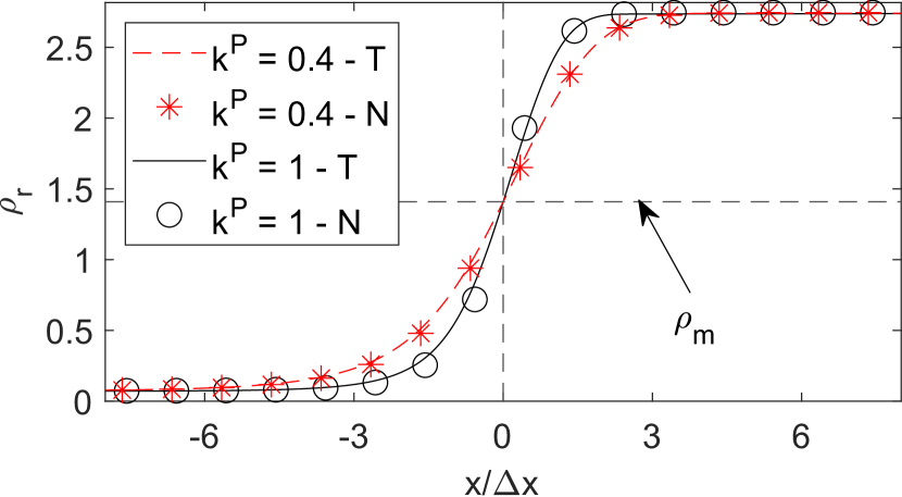
Figure 1: MP-LBM density profile with $\kappa^{P}=0.4$ and $\kappa^{P}=1$ for the C-S EOS with $a=0.5$ l.u. and $T_{r}=0.7$. Symbol T means theoretical results, N numerical and $\rho_{m}=(\rho_{v}+\rho_{l})/2$.

Figure (1) shows the results considering two values of $\kappa^{P}$. First, we observe that the change in the $\kappa^{P}$ successfully changes the interface width without affect the equilibrium densities of each phase. Second, the LBM numerical results showed good agreement with the theoretical solution obtained from solving numerically Eq. (17). Since, the MP-LBM is the only pseudopotential scheme that will be used in the next examples, we will refer to that only as P-LBM.

V Results

V.1 Static planar interface

The first test consists in simulating the equilibrium of two phases separated by a planar interface. After the system reaches the equilibrium, the densities obtained in the numerical simulations will be compared with the Maxwell-rule. Although it was presented theoretical predictions for the equilibrium densities, Eq. (18) for the P-LBM and Eq. (27) for the FE-LBM, they do not guarantee that the numerical models will be able to full recover these values in the simulations. Since we are working with numerical methods, discretization errors can influence the method solution.

To better understand the method behaviour, we need theoretical predictions that will take into account the discretization errors. Those errors could be obtained from the LBE through a Chapman-Enskog analysisChapman and Cowling (1990); Krüger et al. (2017) or by recursive substitutions Lycett-Brown and Luo (2015). However, these procedures are very difficult to be performed for higher orders. An easier approach consists in obtain a discrete equation in terms of the macroscopic properties Peng et al. (2020); Guo (2021). Then, this equation can be easily expanded using Taylor series until any desired order. We followed this approach and derived more precise expressions for the mechanical stability condition for the FE-LBM and P-LBM. The derivations are presented in the Supplementary Material Appendix D and E, respectively.

Following the derivation presented in the Supplementary Material Appendix D, we reach in the following equation for the FE-LBM planar interface (assuming $\tau_{\nu}=\tau_{e}$):

$$\int_{\rho_{v}}^{\rho_{l}}(p_{EOS}-p_{0})\frac{d\rho}{\rho^{2}}=O({\Delta x}^{4}).$$ (34)

Which means that Eq. (27) is an approximation of at least order $O({\Delta x}^{4})$. A similar theoretical analysis is performed with the P-LBM (also using the simplifying assumption $\tau_{\nu}=\tau_{e}$), the details are presented in the Supplemental Material Appendix E. From the analysis, it is concluded that:

$$\int_{\rho_{v}}^{\rho_{l}}(p_{EOS}-p_{0})\frac{\dot{\bar{\psi}}}{\bar{\psi}^{1+\epsilon}}d\rho=O({\Delta x}^{2}),$$ (35)

where $\bar{\psi}=\Delta x\psi$ was adopted to eliminate the influence of $\Delta x$ in the definition of $\psi$, Eq. (11). We observe that the discretization errors in the P-LBM mechanical stability condition are of second order while, for the FE-LBM - Eq. (34) - they are of fourth order. This fact potentially can make the errors in the P-LBM be higher than the FE-LBM.

To validate the theoretical analysis, numerical simulations of a planar interface were performed. A domain of $L_{x}=100\Delta x$ was considered. In FE-LBM, we set $A=0$ and all $\tau$ are equal to $\Delta t$, except $\tau_{e}$, which is equal to $0.75\Delta t$. These choices result in $\nu=c_{s}^{2}\Delta t/2$ and $\nu_{B}=c_{s}^{2}\Delta t/3$. For the P-LBM, we set $\tau_{\nu}=\Delta t$ and $\tau_{e}=\Delta t$, which provide the same values of $\nu$ and $\nu_{B}$ used in the FE tests . The value of $\kappa=0.5$ l.u. was adopted in the FE-LBM and all other P-LBM parameters were chosen to match the FE simulation. The planar interface density profile was initialized using the same procedure as Czelusniak et al.Czelusniak et al. (2020). Results for $a=0.25$ l.u. and $a=0.5$ l.u. in the C-S EOS are presented in Fig. (2) and compared with the Maxwell-rule.

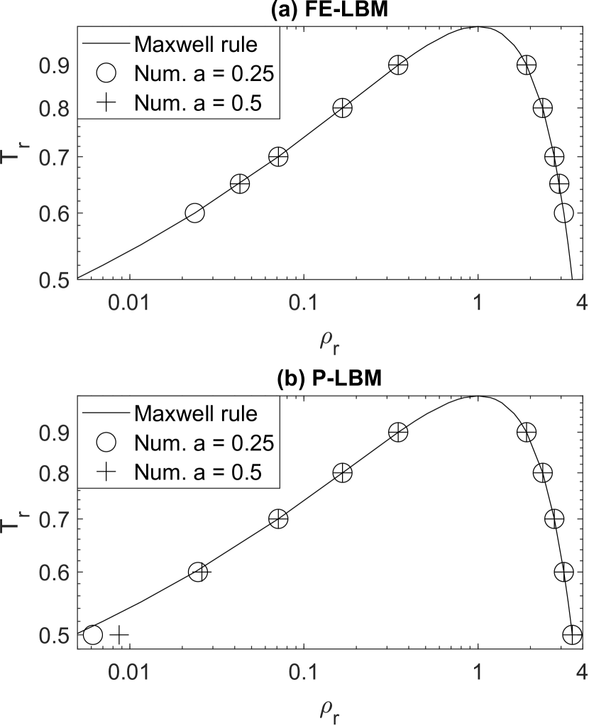
Figure 2: Comparison between numerical (Num.) results and the Maxwell-rule for the C-S EOS with $a=0.25$ l.u. and $a=0.5$ l.u. (a) FE-LBM with $\kappa=0.5$ l.u. (b) P-LBM with parameters adjusted to match FE-LBM.

As expected from the theoretical analysis, in equilibrium, the FE-LBM results - displayed in Fig. (2.a) - are in close agreement to the Maxwell rule. However, the lower stable temperature was $T_{r}=0.65$ for $a=0.5$ l.u. and $T_{r}=0.6$ for $a=0.25$ l.u., evidencing an stability issue. Zhou and HuangZhou and Huang (2023) were able to achieve a temperature of 0.55 for the WB-FE-LBM with a different choice of parameters.

Regarding the P-LBM results displayed in Fig. (2.b) we see that the method is stable for $T_{r}=0.5$ (lower $T_{r}$ were not tested) for both $a$ values in C-S EOS. For $T_{R}$ lower than 0.6, the method starts to loose accuracy due to discretization errors. For these lower temperatures, we conclude that we cannot use the $\sigma^{Li}$ values obtained theoretically from the mechanical stability condition. Unless we write a code to compute the theoretical solution considering a more accurate version of the mechanical stability condition (which we consider a cumbersome process), these $\sigma^{Li}$ values must be obtained empirically running previous LBM simulations.

Next, we evaluate the effect of varying $\tau_{\nu}$ in respect to $\tau_{e}$ and how it affects the equilibrium densities. For this analysis we defined the error of the vapor density in respect to the given by Maxwell rule $\epsilon_{v}=100|\rho_{v}^{\text{N}}-\rho_{v}^{\text{M}}|/\rho_{v}^{\text{M}}$, where $\rho_{v}^{\text{N}}$ is the numerical vapor density obtained in simulation and $\rho_{v}^{\text{M}}$, the Maxwell rule vapor density. The results of this test are presented in Table (1). As we can realize, for the FE-LBM, the vapor error was not affected by the change of $\tau_{v}$ in respect to $\tau_{e}$.

Table 1: Vapor density error in percentage for different $\tau_{\nu}^{\ast}=\tau_{\nu}/\Delta t$. In FE-LBM all other $\tau$ are equal to $\Delta t$ and $A=0$. In P-LBM $\tau_{q}$ was also varied and the other $\tau$ are equal to $\Delta t$. Other simulation parameters are $T_{r}=0.65$, $a=0.5$ l.u. and $\kappa=0.5$ l.u. The value of $\kappa^{Li}$ is equal to zero and $\kappa^{P}$ is adjusted to maintain the same interface width of FE-simulations.

-	$\tau_{\nu}^{\ast}=0.55$	$\tau_{\nu}^{\ast}=0.75$	$\tau_{\nu}^{\ast}=1$	$\tau_{\nu}^{\ast}=1.2$
FE-LBM $\tau_{q}^{\ast}=1$	0.0605	0.0605	0.0605	0.0605
P-LBM $\tau_{q}^{\ast}=1$	50.6	40.0	27.6	18.4
P-LBM $\tau_{q}^{\ast}=1/1.99$	27.7	27.7	27.6	27.6

For the pseudopotential method we observe a large variation of vapor density in respect to $\tau_{\nu}$. This problem was reported by Wu et al.Wu et al. (2018). The authors proposed a correction for this issue which consists in adopting $\tau_{q}=\Delta t/1.99$. We tested this approach and the results are in third line of Table 1. We conclude that this strategy really solves the problem.

V.2 Static Droplet

To evaluate the performance of the methods for curved interfaces, static droplet tests were performed. First, we compare the surface tension measured in the numerical tests (by applying the Young-Laplace law) with the theoretical one (described in Supplementary Material Appendix B). Then, the equilibrium densities of the static droplet tests are compared with the thermodynamic consistent results. These theoretical densities can be computed using the procedure described in Czelusniak et al.Czelusniak et al. (2020), which is different from the Maxwell rule.

Numerical simulations of a 2D static droplet were performed. A domain of $L_{x}=L_{y}=120\Delta x$ was used. For the FE-LBM we set $\kappa=0.5$ l.u., $A=0$ and all $\tau$ equal to $\Delta t$, except $\tau_{e}$ which is equal to $0.75\Delta t$. These choices result in $\nu=c_{s}^{2}\Delta t/2$ and $\nu_{B}=c_{s}^{2}\Delta t/3$. Also, $a=0.25$ l.u. in the C-S EOS. The initialization procedure is similar to the one used by Czelusniak et al.Czelusniak et al. (2020).

The P-LBM test was set similarly to the FE-LBM. Here we set all $\tau=\Delta t$ with the exception of $\tau_{q}=\Delta t/1.99$ to avoid the issues discussed in the previous subsection. The values of $\kappa^{\text{P}}$ and $\kappa^{\text{Li}}$ were adjusted to guarantee that the P-LBM has the same interface width and surface tension than for the FE-LBM simulations.

The pressure difference from inside to outside the droplet was measured and the results for different reduced temperatures and radiuses are shown in Fig. (3). The numerical results presented excellent agreement with the theoretical solution for both methods.

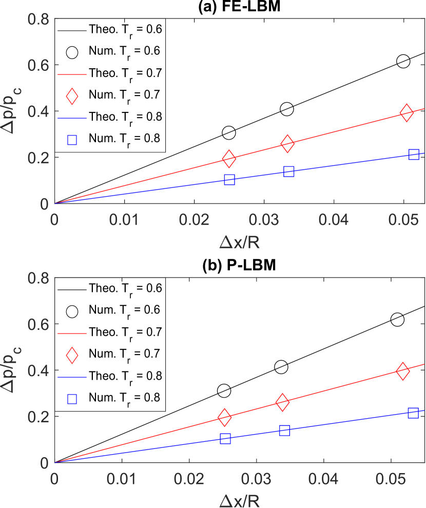
Figure 3: Young-Laplace test comparing numerical (Num.) and theoretical (Theo.) results for the C-S EOS with $a=0.25$ l.u. (a) FE-LBM with $\kappa=0.5$ l.u. (b) P-LBM with parameters selected to match the FE-LBM simulations.

Next, we compare the densities obtained in the numerical tests with the theoretical thermodynamic consistent densities. To expose the results in a concise way, we defined the reduced vapour density difference between the vapor phase density measured in the droplet test $\rho_{v}$ and the vapour density for the planar interface test $\rho_{v}^{\text{PI}}$ as $\Delta\rho_{v}=\rho_{v}-\rho_{v}^{\text{PI}}$ for the same temperature.

The case $\Delta x/R=0$ correspond to a planar interface, then $\Delta\rho_{v}=0$. When we increase $\Delta x/R$, the pressure difference between inside and outside the droplet starts to increase and the vapor density of the droplet test will deviate from the one obtained in the planar interface. In Fig. (4.a) we show the comparison between FE-LBM numerical and theoretical results. The agreement was excellent and the conclusion is that FE-LBM is thermodynamic consistent for the droplet test.

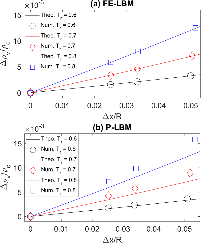
Figure 4: Droplet thermodynamic consistency test comparing numerical (Num.) and theoretica (Theo.) results for the C-S EOS with $a=0.25$ l.u. (a) FE-LBM with $\kappa=0.5$ l.u. (b) P-LBM with parameters adjusted to match FE-LBM simulation. $\Delta\rho_{v}=\rho_{v}-\rho_{v}^{\text{PI}}$ is the vapor difference between the droplet and a planar interface.

Regarding the P-LBM, in Fig. (3.b) the measured surface tension for $T_{r}=0.6$ was close to the theoretical value. However, at this $T_{r}$, the planar interface test showed a discrepancy of 4% in respect to the Maxwell-rule (see Fig. (2.b)). Due to this difference, we decided to find the simulation parameters empirically rather than theoretically at this $T_{r}$. We found that $\epsilon=1.9168$, $\kappa^{\text{Li}}=-1.70$ and $\kappa^{P}=0.919$ provide an appropriate match between the planar interface results from P-LBM and from FE-LBM (considering $\kappa=0.5$ l.u. in FE-LBM).

The droplet densities for the P-LBM are shown in Fig. (4.b). We can see that the P-LBM does not match perfectly with the consistent densities. However, the qualitative behaviour in which the vapor density increase with the curvature is reproduced. We also examined the absolute errors of the vapor density. For a droplet radius of $20\Delta x$ at $T_{r}=0.8$, the thermodynamic consistent reduced vapor density is $\rho_{r;v}=\rho_{v}/\rho_{c}=0.1824$, while the numerical density was $0.1786$, an error of approximately $2$%.

This small error contradicts the results presented by Czelusniak et al.Czelusniak et al. (2022) that reported much larger errors for curved interface. However, until now we just analyzed the variation of the vapor density with the droplet radius. Czelusniak et al.Czelusniak et al. (2020) found that the vapor densities in the P-LBM vary in a nonphysical way in respect to the surface tension. When the surface tension is reduced, the vapor density should approach the one obtained in a planar interface. However in the P-LBM the density deviates.

For a droplet at $T_{r}=0.6$, we varied the surface tension by changing the $\kappa^{\text{Li}}$ parameter. The results are presented in Fig. (5). It is clear that the P-LBM was approaching the thermodynamic consistent results in Fig. (4.b) only for that specific choice of surface tension. For other surface tensions, the method largely deviates. For a droplet radius of $20\Delta x$ and surface tension $\gamma=0.0046$ l.u. the numerical reduced vapor density is $0.0355$, while the theoretical one is $0.0251$, giving an error of $41$%.

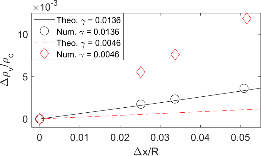
Figure 5: Droplet thermodynamic consistency test with P-LBM for the C-S EOS with $a=0.25$ l.u., $T_{r}=0.6$ and two different surface tensions. $\Delta\rho_{v}=\rho_{v}-\rho_{v}^{\text{PI}}$ is the vapor difference between the droplet and a planar interface.

V.3 Two-phase flow between parallel plates

To evaluate both methods in a flow situation, a two-phase flow between parallel plates was selected. A domain of size $L_{x}=101\Delta x$ and $L_{y}=50\Delta x$ is used. The viscosity is $\nu=c_{s}^{2}\Delta t/2$. The EOS parameters is $a=0.25$ l.u. Initially half of the domain is filled with liquid (top) and the other half is filled with vapor (bottom). No gravity is considered here. A volumetric force in the horizontal direction is applied to drive the flow. The force $F_{x}$ magnitude depends on the simulation temperature: $1\times 10^{-6}$ l.u., $5\times 10^{-7}$ l.u. and $2\times 10^{-7}$ l.u. for $T_{r}$ of 0.8, 0.7 and 0.6, respectively.

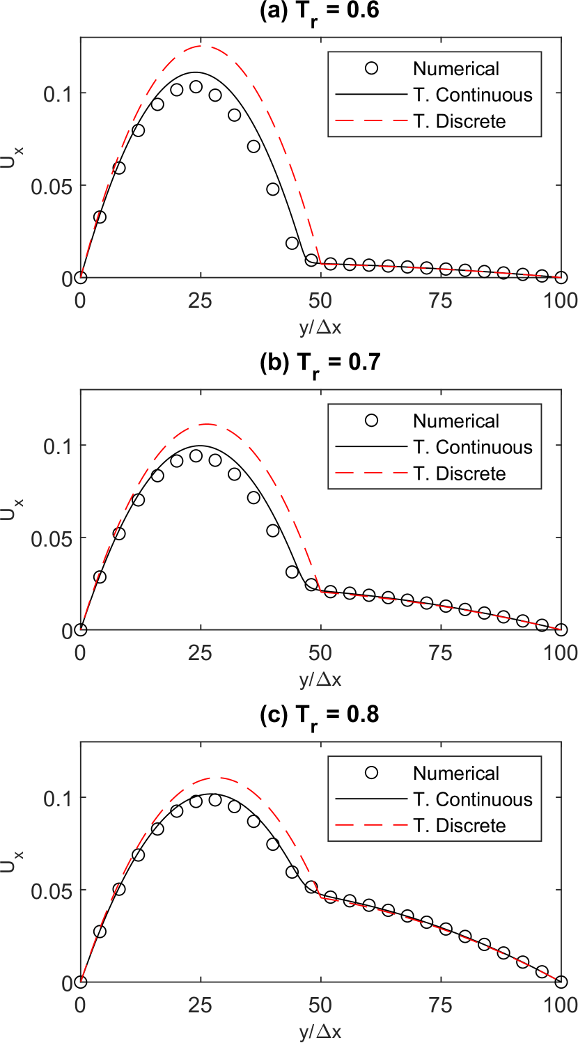
Figure 6: Two-phase flow between parallel plates for FE-LBM ($\kappa=0.5$ l.u.) with the C-S EOS using $a=0.25$ l.u.

Periodic conditions were applied in the side boundaries and no-slipZou and He (1997) were applied in top and bottom boundaries. The relaxation times for P-LBM are $\tau_{\nu}=\Delta t$, $\tau_{e}=\Delta t$ and $\tau_{q}=\Delta t/1.99$. To maintain the same kinematic and bulk viscosities in the FE-LBM we can set $A=0$, $\tau_{\nu}=\Delta t$, $\tau_{e}=0.75\Delta t$. However, we observed that the choice of $\tau_{e}=0.75\Delta t$ in this problem can lead to an unstable simulation. Then, we set $\tau_{e}=\Delta t$ since the bulk viscosity is not important in this particular flow. We also set $\kappa=0.5$ l.u. in FE-LBM and other P-LBM parameters were adjusted to match the same equilibrium densities, interface width and surface tension of the FE-LBM. The density profile is initialized in a similar way to the planar interface test. The initial distribution function is set as equal to the equilibrium one.

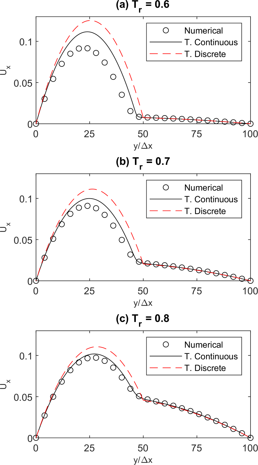
Figure 7: Two-phase flow between parallel plates for P-LBM with the C-S EOS using $a=0.25$ l.u. The P-LBM parameters were set to match the FE-LBM simulation physical properties.

The LBM numerical results can be compared with two types of theoretical solutions. One solution considers a discrete interface and the jump conditions across this interface. However, the LBM is a diffuse interface method and will only approximate the discrete solution in the limit of a vanishing interface thickness. Then, we follow Zhang, Tang, and WuZhang, Tang, and Wu (2022) and use the continuous theoretical solution which take into account the theoretical density profile. Both solutions are described in the Supplementary Material Appendix F.

The FE-LBM results are diplayed in Fig. (6). We observe that LBM indeed approximates better the continuous solution than the discrete one. In the previous tests, the FE-LBM was providing very close approximations to the theoretical solutions in the absence of flow. However, with flow we can observe the effect of numerical errors especially when the temperature is reduced to 0.6.

Before discuss the P-LBM results, recall that in Figs (4) and (5) we used $\sigma^{\text{Li}}$, $\kappa^{P}$ and $\kappa^{\text{Li}}$ obtained empirically rather than theoretically for $T_{r}=0.6$. We did this to compensate the vapor density error in relation to the Maxwell rule. In this test, we will use the parameters obtained theoretically, since we want to do a direct comparison between the method and the theoretical solution.

The P-LBM results are displayed in Fig, (7). We observe that the deviations between the numerical and the theoretical solution are higher in comparison with the FE-LBM. These results suggest that LBM users should consider the necessity of applying a grid refinement procedureJaramillo, Mapelli, and Cabezas-Gómez (2022) to avoid large errors in flow simulations.

Finally, it was also tested a case with $T_{r}=0.5$ and $F_{x}=10^{-7}$ l.u. Only the pseudopotential method resulted in a stable simulation. Due to the lack of comparison between both methods, this case is not presented here.

V.4 Droplet Collision

A dynamic test was select to finish the study: the coalescence of two droplets. We considered a domain of $L_{x}=200\Delta x$ and $L_{y}=100\Delta x$. The viscosities are $\nu=c_{s}^{2}\Delta t/2$ and $\nu_{B}=c_{s}^{2}\Delta t/3$. The EOS parameter is $a=0.25$ l.u. and the simulation occurs at $T_{r}=0.8$. Initially two droplets of diameter $R_{d}=50\Delta x$ are placed at positions $(50\Delta x,50\Delta x)$ and $(150\Delta x,50\Delta x)$.

A force acting in the x-axis of the form $F_{x}=a_{x}|\rho-\rho_{ave}|$ was used to move the droplets towards coalescence, where $\rho_{ave}$ is the average density in the domain. We set the acceleration $a_{x}=5\times 10^{-6}\Delta x(\Delta t)^{-2}$ for $x\leq 100\Delta x$ and $a_{x}=-5\times 10^{-6}\Delta x(\Delta t)^{-2}$ for $x>100\Delta x$. Then, the forces in each side of the domain are in opposite direction and make the droplets approach each other. The force is only applied after a time $t>2000\Delta t$.

The parameters of FE-LBM are $A=0$, $\tau_{\nu}=\Delta t$, $\tau_{e}=0.75\Delta t$ and $\kappa=0.5$. For the P-LBM $\tau_{\nu}=\Delta t$, $\tau_{e}=\Delta t$ and $\tau_{q}=\Delta t/1.99$. Other P-LBM parameters were adjusted to match the same equilibrium densities, interface width and surface tension of the FE-LBM. The droplets density profiles were initialized similarly to the static droplet case. The initial distribution function is considered to be equal to the equilibrium one.

In Fig. (8) we plotted the contours for $\rho_{m}=(\rho_{v}+\rho_{l})/2$ (average density between liquid and vapor) at different dimensionless times $t^{\ast}=t\sqrt{a_{d}/D_{d}}$. First, we observe that both methods provided different results. At $t^{\ast}=1.923$ coalescence was almost beginning for both methods. At $t^{\ast}=1.935$ the droplets in P-LBM already merged into a single droplet, while in the FE-LBM they did not. Only at $t^{\ast}=1.961$ the FE-LBM droplets merged.

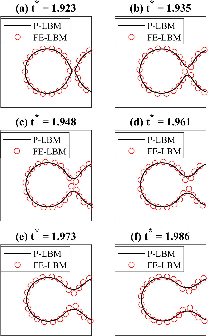
Figure 8: Droplet collision test with P-LBM and FE-LBM for the C-S EOS with $a=0.25$ l.u. and $T_{r}=0.8$.

Next, we decided to compare both simulations but now adding a time delay between them. The P-LBM snapshots are shown at the same time $t^{\ast}$ as in the previous image, while the snapshots of FE-LBM are of time $t^{\ast}+0.0253$. This delay was carefully chosen to make the simulation of both methods merge the droplets together. Then, we can compare the dynamics after merging. These results are presented in Fig. (9).

We observe that both methods provided the same droplet dynamics after merging. These results suggest that the differences between methods only happens before the merging process is complete. More studies are needed to better describe this phenomenon; however, some thoughts can be raised about this.

First, we are initializing the droplets at a certain distance and due to the action of the force they approach each other. In principle the droplets interfaces should get in contact at the same time for both methods. But due to high order discretization errors in both methods, the contact time can differ by a small amount. Since the merging process is very fast as droplets get in contact, if one method starts the merging slightly before, this can produce a visible difference in the method results. So, one possible explanation can be related with the droplets starting the merging at small different times.

Other explanation can be associated with the merging process itself. When two interfaces are merging, the dynamics of this process will be ruled by the pressure tensor of each method. Since both pressure tensors are different, the speed of process can be different for each method.

After that, the dynamics of the simulation will be ruled by properties as surface tension, viscosity and density which are the same for both methods. This explain why results are very similar when we delay simulations to synchronize the merging process.

Finally, we repeat the simulation for other temperatures. We maintain the same $\kappa=0.5$ l.u. for the FE-LBM and adjust the P-LBM parameters to match physical properties with FE method. For $T_{r}=0.7$, the FE-LBM simulation become stable at a certain moment in the merging process. With the P-LBM we were able to produce a stable simulation with $T_{r}=0.6$. We also tested $T_{r}=0.5$ which made the P-LBM unstable. This test also show the superior stability of P-LBM over the well balanced FE-LBM.

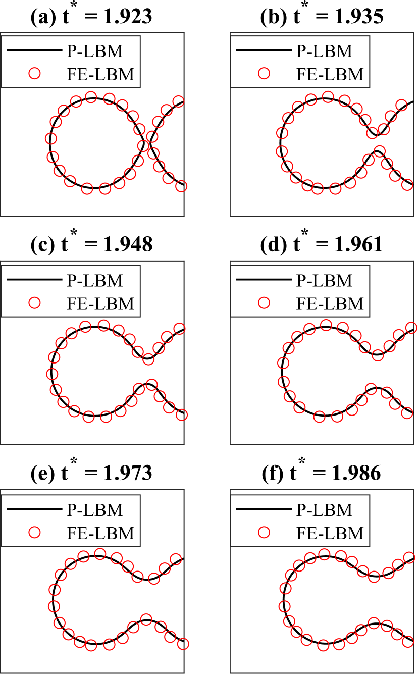
Figure 9: Droplet colision test with P-LBM and FE-LBM for the C-S EOS with $a=0.25$ l.u. and $T_{r}=0.8$. FE-LBM snapshots are delayed by $\Delta t^{\ast}=0.0253$.

VI Conclusion

In this paper we performed a comparison between two methods for multiphase single-component fluid simulations: the pseudopotential (P) and the free energy (FE) lattice Boltzmann methods (LBM). For the FE method we selected the improved well balanced scheme. The equation of state (EOS) considered for this study is the Carnahan-Starling (C-S). We also presented a novel approach to control the interface width of the P-LBM without changing the EOS parameters.

From the planar interface tests, we noticed that the FE-LBM automatically results in the Maxwell rule, while for the P-LBM it is necessary to adjust the $\sigma^{\text{Li}}$ parameter to obtain the correct densities. For a certain range of temperatures it is possible to obtain this parameter theoretically, avoiding a costly empirical trial and error process. However for reduced temperatures of $T_{r}=0.6$ or lower, the theoretical solution do not work well, and an empirical process is necessary any way. In contrast, the P-LBM is more stable than the FE-LBM, which becomes unstable for simulations with $T_{r}=0.6$ or bellow for the choice of parameters in our study.

In droplet tests we observed that the FE-LBM maintains the thermodynamic consistency, while the P-LBM fails. The adjustment carried out with the $\sigma^{\text{Li}}$ parameter in the planar interface test is not enough to guarantee the correct densities for droplets, specially when the surface tension is varied by adjusting the $\kappa^{\text{Li}}$ parameter.

A two-phase flow between parallel plates was simulated to compare both methods in a flow situation. We observed that the FE-LBM do not reproduced the same accuracy showed in the previous tests without flow. However its accuracy was superior compared with the P-LBM. The drop in accuracy for low temperatures indicates that mesh refinement procedures must be considered in simulations of real physical systems.

In the droplet collision simulation, we observed that after the merging of two droplets, the interface dynamics is very similar for both methods. However, it was noticed a difference between methods before merging is complete. Due to this effect, the coalescence process occurs in less time for the P-LBM.

We conclude that the FE-LBM is more practicable and accurate than the P-LBM in the temperature range which it is stable. However, for applications that demand lower reduced temperatures, the FE-LBM can suffer from instability related issues. In this situation, P-LBM takes advantage of its higher stability.

It should be considered that the present comparison was only possible due to the proposed modified P-LBM, that allows to control the interface witdh while maintaining the EOS parameters. This approach made possible the results comparison on the same base. The novel approach is also promising for simulating physical problems employing other EOS under a controlled interface width. This can be important for obtaining numerical solutions of multiphase phase change problems.

Supplementary Material

This paper is accompanied by supplementary material containing 6 appendices mentioned in the text. Appendix A shows the derivation planar interface solutions; Appendix B shows how to compute simulation parameters theoretically; Appendix C shows detailed derivations related to the modified pseudopotential method; Appendix D and E show derivations of planar interface relations with error terms and Appendix F shows solutions for two-phase flow between parallel plates.

Credit Line

The following article has been submitted to Physics of Fluids. After it is published, it will be found at Link .

AUTHOR DECLARATIONS

Conflict of Interest

The authors have no conflicts to disclose.

Data Availability Statement

The data that support the findings of this study are available from the corresponding author upon reasonable request. All the codes used in this work are publicly available at https://github.com/luizeducze/SuppMaterial_Alfa01

References

- Shan and Chen (1993) X. Shan and H. Chen, “Lattice boltzmann model for simulating flows with multiple phases and components,” Physical Review E 47, 1815 (1993).
- Swift et al. (1996) M. R. Swift, E. Orlandini, W. Osborn, and J. Yeomans, “Lattice boltzmann simulations of liquid-gas and binary fluid systems,” Physical Review E 54, 5041 (1996).
- Li, Luo, and Li (2013) Q. Li, K. Luo, and X. Li, “Lattice boltzmann modeling of multiphase flows at large density ratio with an improved pseudopotential model,” Physical Review E 87, 053301 (2013).
- Peng et al. (2020) C. Peng, L. F. Ayala, Z. Wang, and O. M. Ayala, “Attainment of rigorous thermodynamic consistency and surface tension in single-component pseudopotential lattice boltzmann models via a customized equation of state,” Physical Review E 101, 063309 (2020).
- Li and Luo (2013) Q. Li and K. Luo, “Achieving tunable surface tension in the pseudopotential lattice boltzmann modeling of multiphase flows,” Physical Review E 88, 053307 (2013).
- Lycett-Brown and Luo (2015) D. Lycett-Brown and K. H. Luo, “Improved forcing scheme in pseudopotential lattice boltzmann methods for multiphase flow at arbitrarily high density ratios,” Physical Review E 91, 023305 (2015).
- Huang and Wu (2016) R. Huang and H. Wu, “Third-order analysis of pseudopotential lattice boltzmann model for multiphase flow,” Journal of Computational Physics 327, 121–139 (2016).
- Wu et al. (2018) Y. Wu, N. Gui, X. Yang, J. Tu, and S. Jiang, “Fourth-order analysis of force terms in multiphase pseudopotential lattice boltzmann model,” Computers & Mathematics with Applications 76, 1699–1712 (2018).
- Sbragaglia et al. (2007) M. Sbragaglia, R. Benzi, L. Biferale, S. Succi, K. Sugiyama, and F. Toschi, “Generalized lattice boltzmann method with multirange pseudopotential,” Physical Review E 75, 026702 (2007).
- Shan (2006) X. Shan, “Analysis and reduction of the spurious current in a class of multiphase lattice boltzmann models,” Physical Review E 73, 047701 (2006).
- Peng et al. (2019) C. Peng, L. F. Ayala, O. M. Ayala, and L.-P. Wang, “Isotropy and spurious currents in pseudo-potential multiphase lattice boltzmann models,” Computers & Fluids 191, 104257 (2019).
- Li et al. (2015) Q. Li, Q. Kang, M. M. Francois, Y. He, and K. Luo, “Lattice boltzmann modeling of boiling heat transfer: The boiling curve and the effects of wettability,” International Journal of Heat and Mass Transfer 85, 787–796 (2015).
- Fei et al. (2020) L. Fei, J. Yang, Y. Chen, H. Mo, and K. H. Luo, “Mesoscopic simulation of three-dimensional pool boiling based on a phase-change cascaded lattice boltzmann method,” Physics of Fluids 32 (2020).
- Wang, Lou, and Li (2020) H. Wang, Q. Lou, and L. Li, “Mesoscale simulations of saturated flow boiling heat transfer in a horizontal microchannel,” Numerical Heat Transfer, Part A: Applications 78, 107–124 (2020).
- Zhang et al. (2021) C. Zhang, L. Chen, W. Ji, Y. Liu, L. Liu, and W.-Q. Tao, “Lattice boltzmann mesoscopic modeling of flow boiling heat transfer processes in a microchannel,” Applied Thermal Engineering 197, 117369 (2021).
- Li et al. (2021) W. Li, Q. Li, Y. Yu, and K. H. Luo, “Nucleate boiling enhancement by structured surfaces with distributed wettability-modified regions: A lattice boltzmann study,” Applied Thermal Engineering 194, 117130 (2021).
- Wang et al. (2023) J. Wang, G. Liang, X. Yin, and S. Shen, “Pool boiling on micro-structured surface with lattice boltzmann method,” International Journal of Thermal Sciences 187, 108170 (2023).
- Kikkinides et al. (2008) E. Kikkinides, A. Yiotis, M. Kainourgiakis, and A. Stubos, “Thermodynamic consistency of liquid-gas lattice boltzmann methods: Interfacial property issues,” Physical Review E 78, 036702 (2008).
- Wagner (2006) A. Wagner, “Thermodynamic consistency of liquid-gas lattice boltzmann simulations,” Physical Review E 74, 056703 (2006).
- Siebert, Philippi, and Mattila (2014) D. Siebert, P. Philippi, and K. Mattila, “Consistent lattice boltzmann equations for phase transitions,” Physical Review E 90, 053310 (2014).
- Guo (2021) Z. Guo, “Well-balanced lattice boltzmann model for two-phase systems,” Physics of Fluids 33, 031709 (2021).
- Lallemand and Luo (2000) P. Lallemand and L.-S. Luo, “Theory of the lattice boltzmann method: Dispersion, dissipation, isotropy, galilean invariance, and stability,” Physical review E 61, 6546 (2000).
- Krüger et al. (2017) T. Krüger, H. Kusumaatmaja, A. Kuzmin, O. Shardt, G. Silva, and E. M. Viggen, “The lattice boltzmann method,” Springer International Publishing 10, 4–15 (2017).
- Guo, Zheng, and Shi (2002) Z. Guo, C. Zheng, and B. Shi, “Discrete lattice effects on the forcing term in the lattice boltzmann method,” Physical review E 65, 046308 (2002).
- Chapman and Cowling (1990) S. Chapman and T. G. Cowling, The mathematical theory of non-uniform gases: an account of the kinetic theory of viscosity, thermal conduction and diffusion in gases (Cambridge university press, 1990).
- Shan (2008) X. Shan, “Pressure tensor calculation in a class of nonideal gas lattice boltzmann models,” Physical Review E 77, 066702 (2008).
- Yuan and Schaefer (2006) P. Yuan and L. Schaefer, “Equations of state in a lattice boltzmann model,” Physics of Fluids 18, 042101 (2006).
- Shan and Chen (1994) X. Shan and H. Chen, “Simulation of nonideal gases and liquid-gas phase transitions by the lattice boltzmann equation,” Physical Review E 49, 2941 (1994).
- Callen (1960) H. B. Callen, “Thermodynamics and an introduction to thermostatistics,” John Wiley & Sons, New York (1960).
- Bejan (2016) A. Bejan, Advanced engineering thermodynamics (John Wiley & Sons, 2016).
- Kupershtokh, Medvedev, and Karpov (2009) A. L. Kupershtokh, D. Medvedev, and D. Karpov, “On equations of state in a lattice boltzmann method,” Computers & Mathematics with Applications 58, 965–974 (2009).
- Czelusniak et al. (2020) L. E. Czelusniak, V. P. Mapelli, M. Guzella, L. Cabezas-Gómez, and A. J. Wagner, “Force approach for the pseudopotential lattice boltzmann method,” Physical Review E 102, 033307 (2020).
- Bhatnagar, Gross, and Krook (1954) P. L. Bhatnagar, E. P. Gross, and M. Krook, “A model for collision processes in gases. i. small amplitude processes in charged and neutral one-component systems,” Physical review 94, 511 (1954).
- Zhang, Guo, and Wang (2022) C. Zhang, Z. Guo, and L.-P. Wang, “Improved well-balanced free-energy lattice boltzmann model for two-phase flow with high reynolds number and large viscosity ratio,” Physics of Fluids 34, 012110 (2022).
- Baakeem, Bawazeer, and Mohamad (2021) S. S. Baakeem, S. A. Bawazeer, and A. A. Mohamad, “A novel approach of unit conversion in the lattice boltzmann method,” Applied Sciences 11, 6386 (2021).
- Czelusniak, Cabezas-Gómez, and Wagner (2023) L. E. Czelusniak, L. Cabezas-Gómez, and A. J. Wagner, “Effect of gravity on phase transition for liquid–gas simulations,” Physics of Fluids 35, 043324 (2023).
- Zhou and Huang (2023) Z.-T. Zhou and J.-J. Huang, “Study of single-component two-phase free energy lattice boltzmann models using various equations of state,” Physics of Fluids 35 (2023).
- Czelusniak et al. (2022) L. E. Czelusniak, V. P. Mapelli, A. J. Wagner, and L. Cabezas-Gómez, “Shaping the equation of state to improve numerical accuracy and stability of the pseudopotential lattice boltzmann method,” Physical Review E 105, 015303 (2022).
- Zou and He (1997) Q. Zou and X. He, “On pressure and velocity boundary conditions for the lattice boltzmann bgk model,” Physics of fluids 9, 1591–1598 (1997).
- Zhang, Tang, and Wu (2022) S. Zhang, J. Tang, and H. Wu, “Phase-field lattice boltzmann model for two-phase flows with large density ratio,” Physical Review E 105, 015304 (2022).
- Jaramillo, Mapelli, and Cabezas-Gómez (2022) A. Jaramillo, V. P. Mapelli, and L. Cabezas-Gómez, “Pseudopotential lattice boltzmann method for boiling heat transfer: A mesh refinement procedure,” Applied Thermal Engineering 213, 118705 (2022).