Pencil: Private and Extensible Collaborative Learning without the Non-Colluding Assumption

Abstract

The escalating focus on data privacy poses significant challenges for collaborative neural network training, where data ownership and model training/deployment responsibilities reside with distinct entities. Our community has made substantial contributions to addressing this challenge, proposing various approaches such as federated learning (FL) and privacy-preserving machine learning based on cryptographic constructs like homomorphic encryption (HE) and secure multiparty computation (MPC). However, FL completely overlooks model privacy, and HE has limited extensibility (confined to only one data provider). While the state-of-the-art MPC frameworks provide reasonable throughput and simultaneously ensure model/data privacy, they rely on a critical non-colluding assumption on the computing servers, and relaxing this assumption is still an open problem.

In this paper, we present Pencil, the first private training framework for collaborative learning that simultaneously offers data privacy, model privacy, and extensibility to multiple data providers, without relying on the non-colluding assumption. Our fundamental design principle is to construct the $n$-party collaborative training protocol based on an efficient two-party protocol, and meanwhile ensuring that switching to different data providers during model training introduces no extra cost. We introduce several novel cryptographic protocols to realize this design principle and conduct a rigorous security and privacy analysis. Our comprehensive evaluations of Pencil demonstrate that (i) models trained in plaintext and models trained privately using Pencil exhibit nearly identical test accuracies; (ii) The training overhead of Pencil is greatly reduced: Pencil achieves $10\sim 260\times$ higher throughput and 2 orders of magnitude less communication than prior art; (iii) Pencil is resilient against both existing and adaptive (white-box) attacks.

I Introduction

Recent years witnessed significant development and applications of machine learning, in which the most successful ones were the use of deep neural networks. Effective training of neural network models hinges on the availability of a substantial corpus of high-quality training data. However, in real-world business scenarios, the entities possessing data (i.e., data providers, DOes) and the entity seeking to utilize data for training and deployment of a machine learning model (i.e., a model deployer, MO) are distinct parties. One representative example of this is the collaborative anti-money laundering (AML) [55, 4], where multiple financial organizations (e.g., banks) are interested in training anti-money laundering models based on the cell phone records (more accurately, a range of features engineered from these records) that are owned by the cellular service providers. However, the growing emphasis on data privacy, accompanied by the emergence of stringent regulations and laws such as the General Data Protection Regulation (GDPR) [1], has rendered the direct sharing of raw data across multiple organizations infeasible or even unlawful. Consequently, accessing training data, particularly private-domain data not readily accessible on the public Internet, presents a significant research challenge.

Concretely, the above form of collaborative learning raises a combination of three critical requirements. (i) Data Privacy: the training data of different DOes should be kept confidential. This is the preliminary requirement in privacy-preserving machine learning. (ii) Model Privacy: the trained model is only revealed to the MO (i.e., the MO can perform model inference independently), but not disclosed to the DOes. In real-world business scenarios, the post-training model is proprietary. Thus, model privacy is equally important as data privacy. (iii) Extensibility: because the MO often seeks to train the model with multiple (and heterogeneous) data providers, it is critical to ensure that the MO can incrementally collaborate with different DOes. Concretely, we define the this form of learning paradigm private and extensible collaborative learning.

Over the past few years, our community has proposed significant research in this regard. However, none of the existing frameworks meet our aforementioned requirements. (i) Federated Learning (FL) is a widely applied collaborative learning scheme that enables many participants to collectively train a model without sharing their original data. However, the model in FL is synchronized with every participant in every round of the global model update (e.g., [39, 10, 9, 32, 21, 19, 28, 37]). Thus, in FL, the model privacy is simply ignored. (ii) The second stream of approaches relies on secure multiparty computation (MPC) framework, where the DOes upload their data as secret shares to several third-party computing servers (e.g., [43, 56, 24, 51, 42, 3, 41, 59, 47, 11, 33]). The privacy and security guarantees of these proposals require a critical non-colluding assumption that the number of colluding servers must be below a threshold. In fact, in most of these proposals, two colluding servers are sufficient to break the protocol. Thus, the recent SoK on cryptographic neural-network computation [44] considers that “realizing high-throughput and accurate private training without non-colluding assumptions” the first open problem. A strawman design to relax the non-colluding assumption is adopting the $n$-out-of-$n$ sharing schemes [15, 13] in which all the DOes and the MO participate as the computing servers. Yet, the training efficiency is significantly limited (see quantitative results in § VI-E).

I-A Our Contributions

In this paper, we present Pencil , a novel system that meets all three aforementioned requirements of private and extensible collaborative learning, without the non-colluding assumption. At its core, Pencil reduces the multi-party collaborative learning scenario into the 2-party server/client computation paradigm: at each training step, the MO could choose any one of the DOes to collaborate with, and switching between DOes in different training steps introduces no extra cost. This learning protocol is fundamentally different from the existing MPC-based designs that exhibit a tradeoff between non-collusion and extensibility. Specifically, if the MO and DOes choose to secretly share their model and data to third-party MPC servers, extensibility is achieved as the data from multiple DOes can simultaneously contribute to the training, yet they require non-collusion among these third-party MPC servers (e.g., [42, 3, 41, 59, 47, 11, 33]). On the contrary, the MO and DOes can avoid the non-collusion assumption by (i) acting as the computing servers themselves and (ii) adopting the $n$-out-of-$n$ secret sharing schemes [15, 13], which, however, sacrifices extensibility because including additional DOes will significantly increase the time and communication overhead. Pencil eliminates the tradeoff between non-collusion and extensibility by constructing a secure multi-DOes-single-MO training process using our 2-party server/client training protocol (thus relaxing the non-collusion assumption), and meanwhile enabling the MO to securely obtain model weights after each training step so that it can switch to an arbitrary DO in the next training step (thus realizing extensibility).

At a very high level, our 2-party training protocol tactically combines the primitives of the 2-party secure computation protocols and Homomorphic Encryption (HE) cryptosystem for efficient non-linear and linear computation, respectively. Specifically, based on the recent development of efficient private inference [25, 22], we achieve efficient private training by constructing novel cryptography protocols to support backpropagation (such as efficient computation of the product of two secret-shared tensors in computing weight gradient). To further improve training efficiency, we propose a novel preprocessing design to pre-compute heavy HE-related operations (e.g., matrix multiplications and convolutions) offline. This preprocessing design is fundamentally different from the preprocessing technique in [40] that, given a fixed model, accelerates the private inference for a single input sample. Finally, as a contribution independent of our training protocols, we implement the key operators in the BFV HE cryptosystem ([18, 6]) on GPU. By fully exploiting the parallelism in the math construction, our open-sourced prototype achieves, on average, $10\times$ speedup compared with the CPU based implementation of SEAL [52].

In summary, our contributions are:

• We develop Pencil, an efficient training framework to realize efficient collaborative training for the single-MO-multi-DOes scenario. Pencil protects data privacy against the MO and model privacy against the DOes, without requiring the non-colluding assumption. Pencil supports both training from scratch and fine-tuning on existing models.

• We design a set of novel protocols in Pencil, and provide rigorous analysis to prove their security/privacy guarantees. Independent of our protocols, we implement a full GPU version of the BFV HE cryptosystem that is usable by any HE-based machine learning applications.

• We extensively evaluate Pencil. Our results show that: (i) models trained in Pencil and trained in plaintext have nearly identical test accuracies; (ii) With our protocol and hardware optimizations, the training (from scratch) of simple convolutional networks in Pencil converges within 5 hours for the MNIST task. With transfer learning, a complex classifier (e.g., ResNet-50 with 23 million parameters) could be fine-tuned in Pencil within 8 hours for the CIFAR10 task. These results show non-trivial performance improvements over closely related art; (iii) Pencil is extensible to multiple DOes with no overhead increase. In the case where individual DOes possess heterogeneous or even biased datasets, Pencil demonstrates significant performance gains by incorporating more DOes; (iv) we also experimentally show that Pencil is robust against existing attacks and adaptive (white-box) attacks designed specifically for our protocols.

I-B Related Work

The increasingly growing data collaboration among different parties sparked significant research in privately training machine learning models. We divide prior art into three subcategories, as summarized in Table I.

Federated learning (FL) is the pioneering machine learning scheme that treats training data privacy as the first-class citizen. In (horizontal) FL (e.g., [39, 10, 9, 32, 21, 19, 37]), each client (i.e., DO) trains a local model on its private data, and then submits the obfuscated local models to the model aggregator (i.e., MO). Due to the model synchronization in each training iteration, the privacy of the global model is overlooked by FL. In particular, FL disproportionately benefits DOes because each DO learns the global model even if it only partially contributes to the training. As a result, in the case where the MO has an (exclusive) proprietary interest in the final model, FL is not the turnkey solution.

To simultaneously protect data and model privacy, the community proposed a branch of distributed training approaches based on secure multiparty computation (MPC, e.g., [42, 3, 41, 59, 47, 11, 33, 14]). The common setting studied in this line of art is a server-assisted model where a group of DOes upload secret-shared version of their private data to (at least two) non-colluding third-party computing servers to collectively train a model on the secret-shared data. The model is also secret-shared among all servers during the training process, perfectly protecting model privacy. As explained before, this type of approaches suffers from a critical tradeoff between non-collusion and extensibility.

The third subcategory of research depends on homomorphic encryption (HE). These works (e.g., [43, 24, 51, 56]) typically focus on outsourced training where a DO employs a cloud service to train a model by uploading homomorphically-encrypted data, and the final model trained on the cloud is also encrypted. Afterward, the trained model is handed over to the DO or deployed on the cloud as an online inference service usable by the DO. This paradigm, however, is ill-suited in the single-MO-multi-DOes collaborative learning scenario because the plaintext model is not available to the MO for deployment, let alone being further fine-tuned using other DOes’ data (since it requires different HE public/secret key sets).

Differential privacy (DP) is a general technique that can be combined with the aforementioned techniques in private learning. For instance, DPSGD [2] could be used in FL to protect the privacy of individual data points. To defend against gradient matching attacks [63], Tian et al. [56] combines the HE approach with DP mechanics to randomize the weight updates against the cloud service provider. As shown in § III-B2, Pencil allows the DOes to (optionally) add perturbations to the weight updates to achieve additional differential-privacy guarantees on their training data.

[b] Category Representative framework Techniques used^* Data privacy Model privacy Against collusion Extensibility Horizontal FL [39, 10, 9] Local SGD $\checkmark$ $\times$ $\checkmark$ $\checkmark$ Vertical FL [21, 19, 28] Local SGD $\checkmark$ $\times$ $\checkmark$ $\checkmark$ MPC (2 servers) [3, 42] GC, SS $\checkmark$ $\checkmark$ $\times$ $\checkmark$^$\dagger$ MPC (3 servers) [41, 47, 59] GC, SS $\checkmark$ $\checkmark$ $\times$ $\checkmark$^$\dagger$ MPC (4 servers) [11, 33, 14] GC, SS $\checkmark$ $\checkmark$ $\times$ $\checkmark$^$\dagger$ MPC ($n$ servers) [15, 13] GC, SS $\checkmark$ $\checkmark$ $\checkmark$ $\checkmark$^$\ddagger$ Data outsourcing / cloud [43, 24] HE $\checkmark$ $\times$ N/A $\times$ Data outsourcing / cloud [56] HE, DP $\checkmark$ $\times$ N/A $\times$ Pencil Ours HE, SS, DP $\checkmark$ $\checkmark$ $\checkmark$ $\checkmark$

• SGD is for stochastic gradient descent, GC for garbled circuits, SS for secret sharing, HE for homomorphic encryption and DP for differential privacy.

• If MO and DOes choose to secretly share their model and data to third-party MPC servers, extensibility is achieved but the approaches are secure only if these servers are not colluding with each other.

• The general $n$-PC protocol against collusion suffers from a scalability problem: including more parties would greatly increase the computation overhead. See § VI-E for experimental results.

TABLE I: Comparison of prior art related with private collaborative training.

I-C Assumptions and Threat Model

We consider the scenario where one MO and multiple DOes participate in a collaborative machine learning system. All parties are semi-honest, and any of them may collude to infer the private information (model parameters of MO or the data owned by the DOes) of other parties. The architecture of the learning model is known by all parties. As described in the previous sections, we reduce this $n$-party setting to the $2$-party paradigm where only the MO and one of the DOes interact at one single training step. By establishing our privacy guarantees over the two-party protocols, we obtain the security for the general $n$-party extensible machine learning scheme without the non-colluding assumption.

During training, a DO obtains the model prediction result of its own training dataset. Like previous works [51, 25, 41, 33], we do not consider inference attacks based solely on prediction results (e.g., [57, 53]).

II Preliminaries

II-A Notations

Vectors, matrices and tensors are denoted by boldfaced Latin letters (e.g., $\mathbf{W},\mathbf{x})$, while polynomials and scalars are denoted by italic Latin letters (e.g., $W,x$). All the gradients are relative to the loss function $L$ of the deep learning task, i.e., $\nabla_{W}=\nabla_{W}L=\partial{L}/\partial{W}$. $[B]$ denotes the integer interval $[0,B)\bigcap\mathbb{Z}$. Symbol $\mathbf{x}^{\prime}\sim\mathbf{x}$ means that tensor $\mathbf{x}^{\prime}$ is of the same shape as $\mathbf{x}$. If not explicitly specified, a function (e.g., $\mathsf{ReLU}$) applied to a tensor is the function applied to all of its elements.

II-B Lattice-based Homomorphic Encryption

Pencil uses the BFV leveled homomorphic encryption cryptosystem based on the RLWE problem with residual number system (RNS) optimization [18, 6]. In detail, the BFV scheme is constructed with a set of parameters $\{N,t,q\}$ such that the polynomial degree $N$ is a power of two, and $t$, $q$ represent plaintext and ciphertext modulus, respectively. The plaintext space is the polynomial ring $\mathcal{R}_{t,N}=\mathbb{Z}_{t}[X]/(X^{N}+1)$ and the ciphertext space is $\mathcal{R}_{q,N}^{2}$. Homomorphism is established on the plaintext space $\mathcal{R}_{t,N}$, supporting addition and multiplication of polynomials in the encrypted domain. We denote the homomorphically encrypted ciphertext of polynomial $x$ as $[\![x]\!]$. For a tensor $\mathbf{x}$, encryption $[\![\mathbf{x}]\!]$ requires an encoding method to first convey the tensor into the polynomial ring, which we cover in Appendix -A.

II-C Additive Secret Sharing and Fixed-point Representation

We utilize the additive secret-sharing scheme upon the ring $\mathbb{Z}_{t}$ (integers modulo $t$) with $t=2^{\ell}$. If an integer $x\in\mathbb{Z}_{t}$ is shared between a pair of MO and DO, then MO (Party 0) has $\left\langle x\right\rangle_{0}$ and DO (Party 1) has $\left\langle x\right\rangle_{1}$ such that $x=\left\langle x\right\rangle_{0}+\left\langle x\right\rangle_{1}$. For simplicity, $\left\langle x\right\rangle$ denotes $x$ is shared between the two parties.

Machine learning typically involves decimal numbers rather than integers. To adapt to the BFV scheme and integer-based secret sharing, we use a fixed-point representation of decimal numbers. A decimal $\tilde{x}\in\mathbb{R}$ is represented as an integer $x=\mathsf{Encode}(\tilde{x})=\lfloor\tilde{x}\cdot 2^{f}\rfloor\in\mathbb{Z}$, with a precision of $f$ bits. After every multiplication, the precision inflates to $2f$, and a truncation is required to keep the original precision. Since we use $\mathbb{Z}_{t}$ rather than $\mathbb{Z}$, we require all intermediate results in their decimal form $\tilde{x}\in\mathbb{R}$ not to exceed $\pm t/2^{2f+1}$, to prevent overflow. In the rest of the paper, unless stated otherwise, all scalars and elements of tensors are in $\mathbb{Z}_{t}$.

II-D Neural Network Training

A typical neural network (NN) consists of several layers, denoted by a series of functions $f_{i}(\mathbf{x}),i\in{1,2,\cdots,\ell}$, and for an input sample $\mathbf{x}$, the neural network’s output is $\mathbf{y}=f_{\ell}(f_{\ell-1}(\cdots f_{1}(\mathbf{x})\cdots))$, i.e., feeding the input through each layer. It is easy to extend the above modeling to neural networks with branches. The NN layers are roughly divided into two categories: linear layers and non-linear layers. Typically, linear layers (e.g., fully connected layers and convolution layers) contain trainable parameters that could be learned from the input samples and their corresponding labels. Given a linear layer $f_{i}(\mathbf{x};\mathbf{W}_{i},\mathbf{b}_{i})$ with trainable parameters weight $\mathbf{W}_{i}$ and bias $\mathbf{b}_{i}$, we denote it as a function $f_{i}(\mathbf{x})$ when there is no confusion.

Forward propagation. Feeding input through each layer is called forward propagation. In forward propagation, linear layers could be abstracted as

$$\mathbf{y}=f(\mathbf{x})=f(\mathbf{x};\mathbf{W},\mathbf{b})=\mathbf{W}\circ\mathbf{x}+\mathbf{b},$$ (1)

where $\circ$ is a linear operator satisfying the following constraint

$$(\mathbf{u}_{0}+\mathbf{u}_{1})\circ(\mathbf{v}_{0}+\mathbf{v}_{1})=\mathbf{u}_{0}\circ\mathbf{v}_{0}+\mathbf{u}_{1}\circ\mathbf{v}_{0}+\mathbf{u}_{0}\circ\mathbf{v}_{1}+\mathbf{u}_{1}\circ\mathbf{v}_{1}.$$ (2)

For example, in fully connected layers, $\circ$ represents the matrix-vector multiplication:

$$\mathbf{x}\in\mathbb{Z}_{t}^{n_{i}},\mathbf{W}\in\mathbb{Z}_{t}^{n_{o}\times n_{i}},\mathbf{b}\in\mathbb{Z}_{t}^{n_{o}},\mathbf{y}=\mathbf{W}\circ\mathbf{x}+\mathbf{b}=\mathbf{W}\cdot\mathbf{x}+\mathbf{b};$$

in 2-dimensional convolution layers, $\circ$ is the convolution operation:

$$\begin{array}[]{c}\mathbf{x}\in\mathbb{Z}_{t}^{c_{i}\times h\times w},\mathbf{W}\in\mathbb{Z}_{t}^{c_{o}\times c_{i}\times s\times s}\\ \mathbf{W}\circ\mathbf{x}=\mathsf{Conv2d}(\mathbf{x};\mathbf{W})\in\mathbb{Z}_{t}^{c_{o}\times(h-s+1)\times(w-s+1)}\\ \end{array}$$

By contrast, the output of non-linear layers (e.g., ReLU function and max pooling layers) is completely determined by the input.

Backpropagation. The goal of training a neural network is to find a set of trained parameters such that some loss function $L(y;t)$ calculated on network output $y$ and ground truth $t$ (labels) is minimized across a dataset $\mathcal{D}=\{(\mathbf{x}_{i},t_{i})\}_{i}$. In practice, one can draw a batch of $B$ input samples $(\mathbf{X},\mathbf{t})=\{(\mathbf{x}_{i},t_{i})\}_{i\in[B]}$ and calculate the mean loss $L=L(\mathbf{Y},\mathbf{t})=\frac{1}{B}L(\mathbf{y}_{i};t_{i})$. Applying the chain rule, one can reversely compute the partial derivative of each trainable weight with respect to $L$, i.e., $\nabla_{\mathbf{W}}=\partial L/\partial\mathbf{W},\nabla_{\mathbf{b}}=\partial L/\partial\mathbf{b}$ and update the weights accordingly. Since the gradients are propagated reversely from the last layer to the first layer, this process is called backpropagation.

III Training in Pencil

In this section, we introduce our core designs to realize private-preserving training of neural networks in Pencil. We begin by introducing the high-level procedure for our 2-party training protocol. Next, we explain the detailed protocols for training linear and non-linear layers. Then, we introduce an optimization method that offloads the computationally heavy operations to an offline phase. Finally, we demonstrate how to extend our methods for 2-PC to the scenario of arbitrary number of DOes.

III-A Pencil Training Overview

In the training phase of Pencil, the DO holds all training data including labels, while the MO holds all trainable parameters. The network architecture is known to both parties. Except for the final output $y$ which is revealed to the DO, all intermediate outputs of each layer are secret-shared between DO and MO.

In the forward propagation, the DO draws a batch of input data $\mathbf{X}=\{\mathbf{x}_{i}\}_{i\in[B]}$ to feed into the neural network, and the corresponding labels are $\mathbf{t}=\{t_{i}\}_{i\in[B]}$. For input $\mathbf{X}$, denote $\mathbf{X}_{0}=\mathbf{X}$. Evaluation of each layer $f_{i}$ is denoted as $\mathbf{X}_{i}=f_{i}(\mathbf{X}_{i-1})$. At the beginning, MO takes $\left\langle\mathbf{X}_{0}\right\rangle_{0}=\mathbf{0}$ and DO takes $\left\langle\mathbf{X}_{0}\right\rangle_{1}=\mathbf{X}$. This is a secret-sharing of $\left\langle\mathbf{X}_{i}\right\rangle=\left\langle\mathbf{X}_{i}\right\rangle_{0}+\left\langle\mathbf{X}_{i}\right\rangle_{1}$ for $i=0$. We keep this invariant form of secret sharing for all layers $f_{i}$. Essentially, $f_{i}$ is a secure computation protocol operating on secret shares: $f_{i}$ takes shares $\left\langle\mathbf{X}_{i-1}\right\rangle$ from the two parties and produces shares $\left\langle\mathbf{X}\right\rangle_{i}$ to both parties such that

$$\left\langle\mathbf{X}_{i}\right\rangle_{0}+\left\langle\mathbf{X}_{i}\right\rangle_{1}=f_{i}(\left\langle\mathbf{X}_{i-1}\right\rangle_{0}+\left\langle\mathbf{X}_{i-1}\right\rangle_{1}).$$

The construction of such a protocol is introduced in § III-B1. The MO reveals the final propagation output $\left\langle\mathbf{Y}\right\rangle_{0}=\left\langle\mathbf{X}_{\ell}\right\rangle_{0}$ to DO, based on which DO reconstructs the prediction result $\mathbf{Y}$ to calculate the loss function $L(\mathbf{Y},\mathbf{t})$.

In the backpropagation, each derivative $\nabla_{\mathbf{X}_{i}}$ is shared:

$$\left\langle\nabla_{\mathbf{X}_{i-1}}\right\rangle_{0}+\left\langle\nabla_{\mathbf{X}_{i-1}}\right\rangle_{1}=(\left\langle\nabla_{\mathbf{X}_{i}}\right\rangle_{0}+\left\langle\nabla_{\mathbf{X}_{i}}\right\rangle_{1})\odot_{x}\frac{\partial f_{i}(\mathbf{X}_{i-1})}{\partial\mathbf{X}_{i-1}}$$

With secret shared values of $\nabla_{\mathbf{X}_{i}}$ and $\mathbf{X}_{i}$, the two parties could collaborate to produce the gradients of trainable parameters in linear layers, i.e., $\nabla_{\mathbf{W}_{i}},\nabla_{\mathbf{b}_{i}}$:

$$\nabla_{\mathbf{b}_{i}} =\nabla_{\mathbf{X}_{i}}\odot_{b}\frac{\partial f_{i}(\mathbf{X}_{i-1};\mathbf{W}_{i},\mathbf{b}_{i})}{\partial\mathbf{b}_{i}}$$

$$\nabla_{\mathbf{W}_{i}} =\nabla_{\mathbf{X}_{i}}\odot_{W}\frac{\partial f_{i}(\mathbf{X}_{i-1};\mathbf{W}_{i},\mathbf{b}_{i})}{\partial\mathbf{W}_{i}}$$

These weight gradients are revealed to MO to update the parameters (introduced in § III-B2). Note that the linear operators $\odot_{x},\odot_{W},\odot_{b}$ could be deduced from the forward propagation formula $f(\mathbf{X}_{i-1})=\mathbf{X}_{i}$, according to the chain rule of derivatives. The challenge in backpropagation is how to reveal the weight gradients $\nabla_{\mathbf{W}_{i}},\nabla_{\mathbf{b}_{i}}$ only to the MO, while protecting the privacy of both intermediate outputs ($\mathbf{X}_{i},\nabla_{\mathbf{X}_{i}}$) and weights themselves ($\mathbf{W}_{i},\mathbf{b}_{i}$).

As a feed-forward network could be decomposed into a series of layers, in the following, we discuss how to evaluate one single layer in the neural network. Since the trainable parameters of a neural network are in linear layers, we mainly focus on the training protocols of linear layers. We address the evaluations of non-linear layers in § III-C.

III-B Linear Protocols

We first introduce the forward propagation and backpropagation protocols of linear layers. For forward propagation, we adopt the recent development of efficient private preference [25, 22, 38] as a strawman design, and then extend it to support batched inference instead of just single inference. Then we elaborate on the gradient computation protocol in the backpropagation.

III-B1 Forward Propagation

Homomorphic evaluations of linear layers are fundamental to enabling privacy-preserving machine learning. We summarize the high-level protocol in Algorithm 1. Note that because the HE ciphertexts are converted to secret-shares after each linear layer evaluation, we need only to support one HE multiplication in the BFV parameters and do not require bootstrapping. $\circ$ is a linear operator that could be decomposed into basic arithmetic addition and multiplications (e.g., matrix multiplication or convolution).

Input: The input $\left\langle\mathbf{X}\right\rangle$ shared between MO and DO; MO holds the weights $\mathbf{W}$ and the bias $\mathbf{b}$.

Output: The output shares $\left\langle\mathbf{Y}\right\rangle$ of $\mathbf{Y}=\mathbf{W}\circ\mathbf{X}+\mathbf{b}$.

1 DO sends encrypted $[\![\left\langle\mathbf{X}\right\rangle_{1}]\!]$ to MO;

2 MO evaluates $[\![\mathbf{W}\circ\mathbf{X}]\!]=\mathbf{W}\circ([\![\left\langle\mathbf{X}\right\rangle_{1}]\!]+\left\langle\mathbf{X}\right\rangle_{0})$ using homomorphic plaintext-ciphertext additions and multiplications;

3 MO chooses random mask $\mathbf{s}$ and calculates $[\![\left\langle\mathbf{Y}\right\rangle_{1}]\!]=[\![\mathbf{W}\circ\mathbf{X}]\!]-\mathbf{s}$; MO sends $[\![\left\langle\mathbf{Y}\right\rangle_{1}]\!]$ back for decryption;

DO outputs $\left\langle\mathbf{Y}\right\rangle_{1}$; MO outputs $\left\langle\mathbf{Y}\right\rangle_{0}=\mathbf{s}+\mathbf{b}$.

Algorithm 1 Evaluation of linear layer $f$

The substantial part of computation in Algorithm 1 lies in evaluating $\mathbf{W}\circ[\![\mathbf{X}]\!]$. Previous art in private NN inference has developed different methods to evaluate $\mathbf{W}\circ[\![\mathbf{X}]\!]$ for matrix-vector multiplication and 2d-convolutions. For example, [29] uses the SIMD support of BFV cryptosystem and designs a hybrid method for ciphertext matrix multiplication and convolution, while [25] and [22] exploit the polynomial homomorphism to efficiently evaluate the ciphertext dot product in linear layers. Note that private inference of [25] is actually forward propagation of batch size $B=1$, but we adapt these primitives to batched inputs with $B>1$. The details are deferred to Appendix -A.

III-B2 Backpropagation

In backpropagation, with secret shares $\left\langle\nabla_{\mathbf{Y}}\right\rangle$, we need to compute three types of gradients, $\nabla_{\mathbf{X}},\nabla_{\mathbf{b}}$ and $\nabla_{\mathbf{W}}$. The gradient of the inputs $\left\langle\nabla_{\mathbf{X}}\right\rangle$ is again secret-shared between two parties, while the gradient of the parameters $\nabla_{\mathbf{W}},\nabla_{\mathbf{b}}$ are revealed only to the MO. Based on Equation (1), we can deduce the formula of these three types of gradients respectively.

Calculation of $\nabla_{\mathbf{X}}$. For $\nabla_{\mathbf{X}}=\frac{\partial f(\mathbf{X};\mathbf{W},\mathbf{b})}{\partial\mathbf{X}}\odot_{x}\nabla_{\mathbf{Y}}=\mathbf{W}\odot_{x}\nabla_{\mathbf{Y}}$, it takes a form similar to the forward propagation procedure: the two parties input secret shares $\left\langle\nabla_{\mathbf{Y}}\right\rangle$ and the MO provides weights $\mathbf{W}$; the output is a linear operation $\odot_{x}$ on $\nabla_{\mathbf{Y}}$ and $\mathbf{W}$, and the output is shared between two parties. Therefore, we can use a protocol similar to Algorithm 1 to calculate the shares $\left\langle\nabla_{\mathbf{X}}\right\rangle$.

Calculation of $\nabla_{\mathbf{b}}$. $\nabla_{\mathbf{b}}=\nabla_{\mathbf{Y}}\odot_{b}\frac{\partial f(\mathbf{X};\mathbf{W},\mathbf{b})}{\partial\mathbf{b}}$ takes the form of summation across all $B$ samples. Therefore, the two parties can perform summation locally on their shares respectively, and the DO sends its share $\left\langle\nabla_{\mathbf{b}}\right\rangle_{1}$ to MO for reconstruction.

Calculation of $\nabla_{\mathbf{W}}$. It is more challenging to calculate $\nabla_{\mathbf{W}}$ and reveal it to the MO without leaking information about $\mathbf{X}$ or $\nabla_{\mathbf{Y}}$, since both operands of $\odot$ are in secret-shared form: (for simplicity we use $\odot$ instead of $\odot_{W}$):

$$\nabla_{\mathbf{W}}=\nabla_{\mathbf{Y}}\odot\frac{\partial f(\mathbf{X};\mathbf{W},\mathbf{b})}{\partial\mathbf{W}}=\nabla_{\mathbf{Y}}\odot\mathbf{X}$$ (3)

A straightforward solution is to let the DO send encrypted $[\![\left\langle\mathbf{X}\right\rangle_{1}]\!]$ and $[\![\left\langle\nabla_{\mathbf{Y}}\right\rangle_{1}]\!]$ to the MO. The MO calculates the gradient in the encrypted domain as

$$[\![\nabla_{\mathbf{W}}]\!]=(\left\langle\nabla_{\mathbf{Y}}\right\rangle_{0}+[\![\left\langle\nabla_{\mathbf{Y}}\right\rangle_{1}]\!])\odot(\left\langle\mathbf{X}\right\rangle_{0}+[\![\left\langle\mathbf{X}\right\rangle_{1}]\!]).$$ (4)

The MO samples random mask $\mathbf{s}$ and sends back perturbed $[\![\nabla_{\mathbf{W}}-\mathbf{s}]\!]$ for decryption (to protect the model update against the DO). The DO finally sends the decryption result and MO could recover plaintext $\nabla_{\mathbf{W}}$.

However, in the above procedure, we need to evaluate multiplication between two ciphertexts, which is much more expensive than ciphertext-plaintext multiplication. We use the linearity of the binary operator $\odot$ to eliminate this requirement. In particular, $\nabla_{\mathbf{W}}$ could be seen as a summation of four terms: two cross terms $\left\langle\nabla_{\mathbf{Y}}\right\rangle_{0}\odot\left\langle\mathbf{X}\right\rangle_{1},\left\langle\nabla_{\mathbf{Y}}\right\rangle_{1}\odot\left\langle\mathbf{X}\right\rangle_{0}$, and two “local” terms $\left\langle\nabla_{\mathbf{Y}}\right\rangle_{0}\odot\left\langle\mathbf{X}\right\rangle_{0},\left\langle\nabla_{\mathbf{Y}}\right\rangle_{1}\odot\left\langle\mathbf{X}\right\rangle_{1}$ which could be calculated locally by the two parties respectively. Therefore, the MO could simply evaluate the cross term

$$[\![\nabla_{\mathbf{W}}^{\mathsf{cross}}]\!]=\left\langle\nabla_{\mathbf{Y}}\right\rangle_{0}\odot[\![\left\langle\mathbf{X}\right\rangle_{1}]\!]+[\![\left\langle\nabla_{\mathbf{Y}}\right\rangle_{1}]\!]\odot\left\langle\mathbf{X}\right\rangle_{0}$$

and sends back $[\![\nabla_{\mathbf{W}}^{\mathsf{cross}}-\mathbf{s}]\!]$ for decryption. The DO then returns the decrypted result $\widetilde{\nabla_{\mathbf{W}}}=\nabla_{\mathbf{W}}^{\mathsf{cross}}-\mathbf{s}+\left\langle\nabla_{\mathbf{Y}}\right\rangle_{1}\odot\left\langle\mathbf{X}\right\rangle_{1}$, and the MO could recover the full $\nabla_{\mathbf{W}}$ by adding its local term $\left\langle\nabla_{\mathbf{Y}}\right\rangle_{0}\odot\left\langle\mathbf{X}\right\rangle_{0}$ and mask $\mathbf{s}$. We illustrate this protocol in Algorithm 2.

Input: MO and DO input secret shares of $\left\langle\mathbf{X}\right\rangle$ and $\left\langle\nabla_{\mathbf{Y}}\right\rangle$.

Output: MO receives $\nabla_{\mathbf{W}}=\nabla_{\mathbf{Y}}\odot\mathbf{X}$.

1 DO sends encrypted $[\![\left\langle\mathbf{X}\right\rangle_{1}]\!],[\![\left\langle\nabla_{\mathbf{Y}}\right\rangle_{1}]\!]$ to MO;

2 MO evaluates

$$[\![\nabla_{\mathbf{W}}^{\mathsf{cross}}]\!]=\left\langle\nabla_{\mathbf{Y}}\right\rangle_{0}\odot[\![\left\langle\mathbf{X}\right\rangle_{1}]\!]+[\![\left\langle\nabla_{\mathbf{Y}}\right\rangle_{1}]\!]\odot\left\langle\mathbf{X}\right\rangle_{0}$$

3 MO chooses random mask $\mathbf{s}$ and sends $[\![\nabla_{\mathbf{W}}^{\mathsf{cross}}-\mathbf{s}]\!]$ back for decryption;

4 DO evaluates

$$\widetilde{\nabla_{\mathbf{W}}}=\nabla_{\mathbf{W}}^{\mathsf{cross}}-\mathbf{s}+\left\langle\nabla_{\mathbf{Y}}\right\rangle_{1}\odot\left\langle\mathbf{X}\right\rangle_{1}$$

5 DO adds a perturbation $\mathbf{e}$ to $\widetilde{\nabla_{\mathbf{W}}}$;

MO finishes by calculating

$$\nabla_{\mathbf{W}}=\widetilde{\nabla_{\mathbf{W}}}+\mathbf{s}+\left\langle\nabla_{\mathbf{Y}}\right\rangle_{0}\odot\left\langle\mathbf{X}\right\rangle_{0}$$

Algorithm 2 Weight gradient $\nabla_{\mathbf{W}}$ calculation

Incorporating Differential Privacy (DP) for Weight Updates. To ensure independent model deployment, weight updates (i.e., $\nabla_{\mathbf{W}},\nabla_{\mathbf{b}}$) should be revealed to MO in plaintext. Recent art [65, 63, 20] argues that these updates may leak private information about the training data. To address this concern, we integrate the DP mechanism into our framework. Specifically, we allow DO to add perturbations to the gradients, as shown in Step 2 of Algorithm 2:

$$\mathbf{e}\leftarrow\mathcal{N}\left(0,\frac{\sigma^{2}C^{2}}{B}\mathbb{I}\right),$$ (5)

where $B$ is the batch size, and $C$ is the estimated the upper bound of L2 norm of the gradients w.r.t. a single sample. This noise term is added to $\widetilde{\nabla_{\mathbf{W}}}$ in Algorithm 2 and to the summation of DO’s own share of $\nabla_{\mathbf{b}}$. At a high level, our design is a secret-shared version of the DPSGD algorithm [2] (by considering $C$ as the bound to clip gradients).

III-C Non-linear Protocols

To evaluate non-linear layers, [25] proposes various MPC-based protocols utilizing OT extension [31, 61]. As [25] focuses on private inference (i.e., forward propagation), we extend their work to enable the backpropagation of gradients through the non-linear layers. Specifically, we implemented the backpropagation functionalities for rectified linear function (ReLU) and 2-dimensional average pooling layers. We also use truncation protocols to support the multiplication of fixed-point secret-shared numbers. For the concrete construction of these protocols, we refer the readers to Appendix -B.

ReLU function. $\mathsf{ReLU}(x)=\max\{0,x\}$ is an activation function widely used in neural networks. In MPC, $\mathsf{ReLU}$ is effectively implemented by a composition of the derivative $\mathsf{DReLU}(x)=\mathbf{1}\{x>0\}$ and a multiplication, as $\mathsf{ReLU}(x)=\mathsf{DReLU}(x)\cdot x$.

To support backpropagation for $\mathsf{ReLU}$, we need to evaluate

$$\nabla_{x}=\mathsf{DReLU}(x)\cdot\nabla_{y}.$$ (6)

We notice that the $\mathsf{DReLU}(x)$ is already calculated in the forward propagation. Its result is secret shared in boolean form between the two parties as $\langle d\rangle_{0}\oplus\langle d\rangle_{1}=d=\mathsf{DReLU}(x),\langle d\rangle_{0},\langle d\rangle_{1}\in\{0,1\}$ where $\oplus$ is logical XOR. Therefore, we store this result in the forward propagation and reuse it in backpropagation to produce the secret shares of $\nabla_{x}$ in Equation (6).

2D Average Pooling Layer. At a high level, the 2D average pooling layer with kernel size $s$ outputs mean value of every adjacent $s\times s$ pixels. We use the division protocol provided by the framework of [25] to support the forward and backward propagation of average pooling layers.

Truncation. Since we use the fixed-point representation in $\mathbb{Z}_{t}$, to avoid overflow, we need to reduce the precision from $2f$ to $f$ bits after every multiplication. In the forward propagation, we truncate the multiplication results of fully connected or convolutional layers after the activation function $\mathsf{ReLU}$. In the backward propagation, the gradients of intermediate outputs $\nabla_{\mathbf{X}}$ are truncated after being propagated through any linear layer.

III-D Preprocessing Optimization

In both forward and backward propagation, we notice that the substantial part of computation lies in the plaintext-ciphertext evaluation of linear operations $\circ$ and $\odot$, i.e., $\mathbf{W}\circ[\![\mathbf{X}]\!]$ in Algorithm 1, and $[\![\nabla_{\mathbf{W}}^{\mathsf{cross}}]\!]=\left\langle\nabla_{\mathbf{Y}}\right\rangle_{0}\odot[\![\left\langle\mathbf{X}\right\rangle_{1}]\!]+[\![\left\langle\nabla_{\mathbf{Y}}\right\rangle_{1}]\!]\odot\left\langle\mathbf{X}\right\rangle_{0}$ in Algorithm 2. These evaluations are performed in every training iteration. We propose an optimization method to reduce the total number of such evaluations required in training. Specifically, originally we need $O(T)$ (number of training iterations) online evaluations, while the optimized approach only performs $O(m^{2})=O(1)$ offline evaluations ($m$ is a constant agreed by the two parties) and is completely free of HE computation in the online phase.

We start by constructing a general protocol $\mathsf{P}(\circ,\mathbf{u},\mathbf{v})$ for calculating the shares of $\mathbf{u}\circ\mathbf{v}$ for any linear operator $\circ$, where $\mathbf{u}$ and $\mathbf{v}$ are private data owned by MO and DO, respectively.

For Fixed $\mathbf{u}$ and Variable $\mathbf{v}$. We first consider a fixed $\mathbf{u}$. Inspired by a series of art [7, 42, 40], we observe that: if for some random $\mathbf{v}^{\prime}$, the product $\left\langle\mathbf{u}\circ\mathbf{v}^{\prime}\right\rangle$ could be evaluated and shared beforehand, then given the real $\mathbf{v}$, two parties can compute $\left\langle\mathbf{u}\circ\mathbf{v}\right\rangle$ without HE at all. This protocol can be summarized as follows:

• Preprocessing phase (prepares shares of $\left\langle\mathbf{u}\circ\mathbf{v}^{\prime}\right\rangle$):

  • DO chooses random mask $\mathbf{v}^{\prime}\sim\mathbf{v}$ and sends $[\![\mathbf{v}^{\prime}]\!]$;

  • MO chooses random mask $\mathbf{s}\sim\mathbf{u}\circ\mathbf{v}$, evaluates $[\![\mathbf{u}\circ\mathbf{v}^{\prime}-\mathbf{s}]\!]=\mathbf{u}\circ[\![\mathbf{v}^{\prime}]\!]-\mathbf{s}$ and sends it back. Thus, the two parties get shares of $\mathbf{u}\circ\mathbf{v}^{\prime}$: $\left\langle\mathbf{u}\circ\mathbf{v}^{\prime}\right\rangle_{0}=\mathbf{s},\left\langle\mathbf{u}\circ\mathbf{v}^{\prime}\right\rangle_{1}=\mathbf{u}\circ\mathbf{v}^{\prime}-\mathbf{s}$.

• Online phase (produces shares of $\left\langle\mathbf{u}\circ\mathbf{v}\right\rangle$):

  • DO sends masked $\mathbf{v}-\mathbf{v}^{\prime}$ to MO, outputs $\left\langle\mathbf{u}\circ\mathbf{v}\right\rangle_{1}=\left\langle\mathbf{u}\circ\mathbf{v}^{\prime}\right\rangle_{1};$

  • MO calculates and outputs $\left\langle\mathbf{u}\circ\mathbf{v}\right\rangle_{0}=\mathbf{u}\circ(\mathbf{v}-\mathbf{v}^{\prime})+\left\langle\mathbf{u}\circ\mathbf{v}^{\prime}\right\rangle_{0}.$

Although this protocol could offload HE operations to the preprocessing phase for a single evaluation of $\mathbf{u}\circ\mathbf{v}$, we cannot extend it to multiple evaluations of $\mathbf{u}\circ\mathbf{v}_{i}$ with different $\mathbf{v}_{i}$. Specifically, if we used the same mask $\mathbf{v}^{\prime}$ for two different $\mathbf{v}_{1}$ and $\mathbf{v}_{2}$, then in the online phase the DO would receive $\mathbf{v}_{1}-\mathbf{v}^{\prime}$, and $\mathbf{v}_{2}-\mathbf{v}^{\prime}$. Thus the difference $\mathbf{v}_{1}-\mathbf{v}_{2}$ would be leaked to MO.

To address this issue, we propose using multiple masks $\mathbf{v}^{\prime}_{i}$. In the preprocessing phase, the two parties generate $m$ shared product $\mathbf{u}\circ\mathbf{v}^{\prime}_{i}$ for different $\mathbf{v}^{\prime}_{i},i\in[m]$. In the online phase, for input $\mathbf{v}$, the DO chooses $m$ non-zero scalars $k_{i}$ and sends a masked version of $\mathbf{v}$,

$$\tilde{\mathbf{v}}=\mathbf{v}-\sum_{i\in[m]}k_{i}\cdot\mathbf{v}^{\prime}_{i}$$ (7)

to MO. The two parties output

$$\left\langle\mathbf{u}\circ\mathbf{v}\right\rangle_{0} =\mathbf{u}\circ\tilde{\mathbf{v}}+\sum_{i\in[m]}k_{i}\cdot\left\langle\mathbf{u}\circ\mathbf{v}^{\prime}_{i}\right\rangle_{0}$$ (8)

$$\left\langle\mathbf{u}\circ\mathbf{v}\right\rangle_{1} =\sum_{i\in[m]}k_{i}\cdot\left\langle\mathbf{u}\circ\mathbf{v}^{\prime}_{i}\right\rangle_{1}$$

For Variable $\mathbf{u}$. Now we consider the case where $\mathbf{u}$ is a variable (i.e., not determined at the preprocessing phase). Similar to DO, MO also masks its $\mathbf{u}$ with $m$ masks $\mathbf{u}^{\prime}_{i}$. The online phase could be viewed as a two-step process: (i) the two parties generate shares $\langle\mathbf{u}\circ\mathbf{v}^{\prime}_{j}\rangle$ for all $j\in[m]$; (ii) they apply these shares to further produce shares $\left\langle\mathbf{u}\circ\mathbf{v}\right\rangle$. We present the full protocol in Algorithm 3. In practice, Step 3 and Step 3 in Algorithm 3 can be merged in parallel, as they are independent.

Input: A predefined linear operation $\circ$; in the online phase, MO inputs $\mathbf{u}$ and DO inputs $\mathbf{v}$.

Output: The two parties receive shares of $\left\langle\mathbf{u}\circ\mathbf{v}\right\rangle$.

1 Preprocessing $\mathsf{P}_{\mathsf{Prep}}(\circ)$:

2 MO selects $m$ random masks $\mathbf{u}^{\prime}_{i}\sim\mathbf{u},i\in[m]$;

3 DO selects $m$ random masks $\mathbf{v}^{\prime}_{j}\sim\mathbf{v},j\in[m]$, and sends their encryption $[\![\mathbf{v}^{\prime}_{j}]\!]$ to MO;

4 MO selects $m^{2}$ masks $\mathbf{s}_{ij}\sim(\mathbf{u}\circ\mathbf{v}),i,j\in[m]$;

5 MO evaluates $[\![\langle\mathbf{u}^{\prime}_{i}\circ\mathbf{v}^{\prime}_{j}\rangle_{1}]\!]=\mathbf{u}^{\prime}_{i}\circ[\![\mathbf{v}^{\prime}_{j}]\!]-\mathbf{s}_{ij}$ for $i,j\in[m]$, and sends them back for decryption;

6 MO and DO keeps shares of $\langle\mathbf{u}^{\prime}_{i}\circ\mathbf{v}^{\prime}_{j}\rangle$ for all $i,j\in[m]$

$$\langle\mathbf{u}^{\prime}_{i}\circ\mathbf{v}^{\prime}_{j}\rangle_{0} =\mathbf{s}_{ij}$$

$$\langle\mathbf{u}^{\prime}_{i}\circ\mathbf{v}^{\prime}_{j}\rangle_{1} =\mathbf{u}^{\prime}_{i}\circ\mathbf{v}^{\prime}_{j}-\mathbf{s}_{ij}$$

7 Online $\mathsf{P}_{\mathsf{Online}}(\circ,\mathbf{u},\mathbf{v})$:

8 MO randomly picks scalars $k_{i},i\in[m]$; MO sends to DO all $k_{i}$ and

$$\tilde{\mathbf{u}}=\mathbf{u}-\sum_{i\in[m]}k_{i}\cdot\mathbf{u}^{\prime}_{i}$$

9 MO and DO produces shares of $\langle\mathbf{u}\circ\mathbf{v}^{\prime}_{j}\rangle$ for all $j\in[m]$ as

$$\langle\mathbf{u}\circ\mathbf{v}^{\prime}_{j}\rangle_{0} =\sum_{i\in[m]}k_{i}\cdot\langle\mathbf{u}^{\prime}_{i}\circ\mathbf{v}^{\prime}_{j}\rangle_{0}$$

$$\langle\mathbf{u}\circ\mathbf{v}^{\prime}_{j}\rangle_{1} =\tilde{\mathbf{u}}\circ\mathbf{v}^{\prime}_{j}+\sum_{i\in[m]}k_{i}\cdot\langle\mathbf{u}^{\prime}_{i}\circ\mathbf{v}^{\prime}_{j}\rangle_{1}$$

10 DO randomly picks scalars $\ell_{j},j\in[m]$; DO sends to MO all $\ell_{j}$ and

$$\tilde{\mathbf{v}}=\mathbf{v}-\sum_{j\in[m]}\ell_{j}\cdot\mathbf{v}^{\prime}_{j}$$

MO and DO produces shares of $\langle\mathbf{u}\circ\mathbf{v}\rangle$ as

$$\langle\mathbf{u}\circ\mathbf{v}\rangle_{0} =\mathbf{u}\circ\tilde{\mathbf{v}}+\sum_{j\in[m]}\ell_{j}\cdot\langle\mathbf{u}\circ\mathbf{v}^{\prime}_{j}\rangle_{0}$$

$$\langle\mathbf{u}\circ\mathbf{v}\rangle_{1} =\sum_{j\in[m]}\ell_{j}\cdot\langle\mathbf{u}\circ\mathbf{v}^{\prime}_{j}\rangle_{1}$$

Algorithm 3 $\mathsf{P}(\circ,\mathbf{u},\mathbf{v})$: Preprocessing optimization for calculating the shares of $\mathbf{u}\circ\mathbf{v}$

For simplicity, we denote Algorithm 3 as a general protocol

$$\mathsf{P}(\circ,\mathbf{u},\mathbf{v})=(\mathsf{P}_{\mathsf{Prep}}(\circ),\mathsf{P}_{\mathsf{Online}}(\circ,\mathbf{u},\mathbf{v})),$$

consisting of a preprocessing protocol $\mathsf{P}_{\mathsf{Prep}}(\circ)$ independent of $\mathbf{u},\mathbf{v}$ and a online protocol $\mathsf{P}_{\mathsf{Online}}(\circ,\mathbf{u},\mathbf{v})$ to specifically evaluate $\mathbf{u}\circ\mathbf{v}$.

Applying $\mathsf{P}(\circ,\mathbf{u},\mathbf{v})$ in Linear Layer Training. We now apply $\mathsf{P}(\circ,\mathbf{u},\mathbf{v})$ to accelerate the online training of linear layers in Algorithm 1 and Algorithm 2. In particular, for every invocation with the same $\circ$ of $\mathsf{P}(\circ,\mathbf{u},\mathbf{v})$, the preprocessing phase $\mathsf{P}_{\mathsf{Prep}}(\circ)$ is executed once and for all, before the training starts. When $\mathbf{u},\mathbf{v}$ come on the fly during training, the two parties only execute $\mathsf{P}_{\mathsf{Online}}(\circ,\mathbf{u},\mathbf{v})$. We present the training protocol optimized by $\mathsf{P}(\circ,\mathbf{u},\mathbf{v})$ in Algorithm 4. For consistency of symbols, we semantically denote $\mathbf{v}\odot_{\mathsf{rev}}\mathbf{u}=\mathbf{u}\odot\mathbf{v}$. We provide the security analysis of this preprocessing optimization technique in § IV.

1 Preprocessing:

2 The two parties invoke $\mathsf{P}_{\mathsf{Prep}}(\circ)$, $\mathsf{P}_{\mathsf{Prep}}(\odot_{x})$, $\mathsf{P}_{\mathsf{Prep}}(\odot)$, $\mathsf{P}_{\mathsf{Prep}}(\odot_{\mathsf{rev}})$.

3 Online:

4

5Foward propagation: MO, DO provide shares of $\left\langle\mathbf{X}\right\rangle$.

6

7 The two parties invoke $\mathsf{P}_{\mathsf{Online}}(\circ,\mathbf{W},\left\langle\mathbf{X}\right\rangle_{1})$ to produce the shares of $\langle\mathbf{W}\circ\langle\mathbf{X}\rangle_{1}\rangle$. MO and DO respectively output

$$\langle\mathbf{Y}\rangle_{0} =\langle\mathbf{W}\circ\langle\mathbf{X}\rangle_{1}\rangle_{0}+\mathbf{W}\circ\langle\mathbf{X}\rangle_{0}+\mathbf{b}$$

$$\langle\mathbf{Y}\rangle_{1} =\langle\mathbf{W}\circ\langle\mathbf{X}\rangle_{1}\rangle_{1}$$

8

9 Backpropagation: MO, DO provide shares of $\left\langle\nabla_{\mathbf{Y}}\right\rangle$.

10

11 (For $\nabla_{\mathbf{X}}$) The two parties invoke $\mathsf{P}_{\mathsf{Online}}(\odot_{x},\mathbf{W},\langle\nabla_{\mathbf{Y}}\rangle_{1})$ to produce shares of $\mathbf{W}\odot_{x}\langle\nabla_{\mathbf{Y}}\rangle_{1}$. MO and DO respectively output

$$\langle\nabla_{\mathbf{X}}\rangle_{0} =\langle\mathbf{W}\odot_{x}\langle\nabla_{\mathbf{Y}}\rangle_{1}\rangle_{0}+\mathbf{W}\odot_{x}\langle\nabla_{\mathbf{Y}}\rangle_{0}$$

$$\langle\nabla_{\mathbf{X}}\rangle_{1} =\langle\mathbf{W}\odot_{x}\langle\nabla_{\mathbf{Y}}\rangle_{1}\rangle_{1}$$

12

13(For $\nabla_{\mathbf{b}}$) The two parties locally compute $\langle\nabla_{\mathbf{b}}\rangle_{0}$ and $\langle\nabla_{\mathbf{b}}\rangle_{1}$. DO add perturbation to its share, and $\nabla_{\mathbf{b}}$ is revealed to MO.

14

15(For $\nabla_{\mathbf{W}}$) The two parties invoke $\mathsf{P}_{\mathsf{Online}}(\odot,\langle\nabla_{\mathbf{Y}}\rangle_{0},\langle\mathbf{X}\rangle_{1})$, $\mathsf{P}_{\mathsf{Online}}(\odot_{\mathsf{rev}},\langle\mathbf{X}\rangle_{0},\langle\nabla_{\mathbf{Y}}\rangle_{1})$ to produce shares of the cross terms $\langle\nabla_{\mathbf{W}}^{\mathsf{01}}\rangle$ and $\langle\nabla_{\mathbf{W}}^{\mathsf{10}}\rangle$:

$$\langle\nabla_{\mathbf{W}}^{\mathsf{01}}\rangle =\langle\langle\nabla_{\mathbf{Y}}\rangle_{0}\odot\langle\mathbf{X}\rangle_{1}\rangle$$

$$\langle\nabla_{\mathbf{W}}^{\mathsf{10}}\rangle =\langle\langle\nabla_{\mathbf{Y}}\rangle_{1}\odot\langle\mathbf{X}\rangle_{0}\rangle=\langle\langle\mathbf{X}_{0}\rangle\odot_{\mathsf{rev}}\langle\nabla_{\mathbf{Y}}\rangle_{1}\rangle$$

16 DO calculates

$$\widehat{\nabla_{\mathbf{W}}}=\langle\nabla_{\mathbf{W}}^{\mathsf{01}}\rangle_{1}+\langle\nabla_{\mathbf{W}}^{\mathsf{10}}\rangle_{1}+\langle\nabla_{\mathbf{Y}}\rangle_{1}\odot\langle\mathbf{X}\rangle_{1}$$

17 DO adds a perturbation $\mathbf{e}$ to $\widehat{\nabla_{\mathbf{W}}}$ and sends it to MO;

MO finishes with

$$\nabla_{\mathbf{W}}=\widehat{\nabla_{\mathbf{W}}}+\langle\nabla_{\mathbf{W}}^{\mathsf{01}}\rangle_{0}+\langle\nabla_{\mathbf{W}}^{\mathsf{10}}\rangle_{0}+\langle\nabla_{\mathbf{Y}}\rangle_{0}\odot\langle\mathbf{X}\rangle_{0}$$

Algorithm 4 Optimized Training Protocol of Linear Layers

III-E Extending to Multiple DOes

In practice, the dataset provided by each DO could be highly heterogeneous or even biased. Thus, it is desirable to simultaneously train a model using the combined data contributed by different DOes.

As stated in § I-B, extensibility is challenging in prior art. For instance, in previous HE-based training protocols ([43, 56]), the MO can only train the model with one DO, because the model is encrypted by the DO. In MPC-based approaches ([42, 41, 11, 33]), if MO and DOes upload their model and data to several fixed computing servers, it would introduce the undesirable “non-colluding” assumption. On the other hand, if the MO and all DOes themselves participate as computing nodes, the MPC scheme would have to defend privacy against up to $n-1$ colluding parties, which would result in low efficiency.

Our framework avoids the high overhead of directly supporting an $n$-party computation by decomposing the procedure into the 2-PC paradigm, as we only need interaction between the MO and one DO at a time. The weights are kept by the MO in plaintext so it could simply conduct collaborative training with each DO in turn and updates its model incrementally. This design makes Pencil extend to more DOes without extra computation or communication overhead, unlike previous general $n$-party MPC methods. In § VI-C3, we evaluate the extensibility of Pencil.

IV Security Analysis

IV-A Security of the Pencil Training Framework

In this section, we first perform the security analysis for the Pencil training framework without the preprocessing optimization described in § III-D.

Definition IV.1.

A protocol $\Pi$ between a DO possessing a train dataset $\mathcal{D}=\{(\mathbf{x}_{i},t_{i})\}$ and a MO possessing the model weights $\mathbf{M}$ is a cryptographic training protocol if it satisfies the following guarantees.

• Correctness. On every set of model weights $\mathbf{M}$ of the MO and every dataset $\mathcal{D}$ of the DO, the output of the MO is a series of weight updates and finally a correctly trained model with updated weights.

• Security.

  • (Data privacy) We require that a corrupted, semi-honest MO does not learn anything useful about the DO’s training data, except the weight updates and the final model. Formally, we require the existence of an efficient simulator $\mathsf{Sim}_{MO}$ such that $\mathsf{View}_{MO}^{\Pi}\approx_{c}\mathsf{Sim}_{MO}(\mathbf{M},\mathsf{out})$, where $\mathsf{View}_{MO}^{\Pi}$ denotes the view of the MO in the execution of $\Pi$, $\mathsf{out}$ denotes the output of the training protocol to MO, and $\approx_{c}$ denotes computational indistinguishability between two distributions.

  • (Model privacy) We require that a corrupted, semi-honest DO does not learn anything useful about the MO’s model weights, except the model’s outputs (predictions) on DO’s dataset. The model architecture is public to all parties. Formally, we require the existence of an efficient simulator $\mathsf{Sim}_{DO}$ such that $\mathsf{View}_{DO}^{\Pi}\approx_{c}\mathsf{Sim}_{DO}(\mathcal{D})$, where $\mathsf{View}_{DO}^{\Pi}$ denotes the view of the client in the execution of $\Pi$.

Theorem IV.1.

Assuming the existence of oblivious transfer, homomorphic encryption and secure protocols for non-linearity evaluations, the Pencil framework without the preprocessing optimization is a cryptographic training protocol as defined in Definition IV.1.

We rigorously prove Theorem IV.1 using the real/ideal word paradigm by constructing simulators for the DO and the MO. Due to space constraint, the detailed simulator construction and hybrid proof are deferred to Appendix -C. Extending the theorem to the single-MO-multi-DOes scenario is trivial.

IV-B Distinguishability Caused by Prepossessing Optimization

After introducing the preprocessing technique (see § III-D) in Pencil, the computational indistinguishability of these views no longer holds. This is because we use linear combinations of $m$ masks for the multiplication operands $\mathbf{u}$ and $\mathbf{v}$ of any linear operator $\circ$, instead of using uniformly random tensor masks. In this section, we analyze and quantify such distinguishability and prove that the privacy loss caused by the distinguishability is negligible (i.e., it is computationally difficult for an adversary to derive private information based on the distinguishability).

We first give a useful proof gadget.

Definition IV.2.

A set $\mathbf{V}=\{\mathbf{v}_{i}\}_{i\in[n]}$ of $n$ elements is $m$-linear combinatorially private to a party S, if any property about the elements in $\mathbf{V}$, derived by S, has the form of a linear combination

$$\sum_{i\in[m^{\prime}]}a_{i}\mathbf{v}_{n_{i}}=\hat{\mathbf{v}}$$ (9)

where $n_{i}$ are $m^{\prime}$ distinct indices in $[n]$ and $m^{\prime}>m$. $a_{i}\neq 0$, $m$, and $\hat{\mathbf{v}}$ are public parameters that are not controlled by S.

Now we present the following theorem.

Theorem IV.2.

If $\mathsf{P}_{\mathsf{Online}}(\circ,\mathbf{u},\mathbf{v})$ (Algorithm 3) is executed $n$ times with $n$ different $\mathbf{u}_{i}$ provided by MO and $n$ different $\mathbf{v}_{i}$ provided by DO, and $m<n<\!\!<t$ ($t$ is the number of elements in the ring $\mathbb{Z}_{t}$), then $\mathbf{U}=\{\mathbf{u}_{i}\}_{i\in[n]}$ are $m$-linear combinatorially private to DO, and $\mathbf{V}=\{\mathbf{v}_{i}\}_{i\in[n]}$ are $m$-linear combinatorially private to MO.

• Since $\mathbf{u}_{i}$ and $\mathbf{v}_{i}$ are symmetric for DO and MO, respectively, proving the theorem for $\mathbf{v}_{i}$ is sufficient. We prove the theorem using the elimination of the masks: since each $\mathbf{v}_{i}$ is masked with $m$ different masks, eliminating every mask requires a new equation of $\tilde{\mathbf{v}}_{i}$ (see Equation 10 below). Thus, the adversary could eventually obtain a linear combination of at least $m+1$ different $\mathbf{v}_{i}$’s in $\mathbf{V}$. The formal formulation is as follows.

  In the preprocessing phase $\mathsf{P}_{\mathsf{Prep}}(\circ)$, DO spawns $m$ random $\mathbf{v}^{\prime}_{j}$. In the online phase $\mathsf{P}_{\mathsf{Online}}(\circ,\mathbf{u}_{i},\mathbf{v}_{i})$, DO chooses $m$ scalars $\ell_{ij}\in\mathbb{Z}_{t}$ for each $\mathbf{v}_{i}$ and sends to MO the following

  $$\tilde{\mathbf{v}}_{i}=\mathbf{v}_{i}-\sum_{j=0}^{m-1}\ell_{ij}\mathbf{v}^{\prime}_{j},i\in[n].$$ (10)

  Let matrix $\mathbf{L}=(\ell_{ij})\in\mathbb{Z}_{t}^{n\times m}$. Since $\ell_{ij}$ are chosen uniformly in $\mathbb{Z}_{t}$ and $n<\!\!<t$, $\mathbf{L}$ is full-rank ($\mathsf{rank}(\mathbf{L})=m$) with high probability [8, 12]. Therefore, in order to eliminate $\mathbf{v}^{\prime}_{j}$ which are unknown to MO, MO needs at least $m+1$ equations in the form of Equation (10) to obtain a linear combination of elements in $\mathbf{V}$. Finally, MO obtains a relation of $m^{\prime}>m$ tensors in $\{\mathbf{v}_{i}\}$ of its choice:

  $$\sum_{k=0}^{m^{\prime}-1}a_{k}\mathbf{v}_{n_{k}}=\hat{\mathbf{v}},$$

  where the linear combination coefficients $a_{k}$ are determined by $\mathbf{L}$, and $\hat{\mathbf{v}}$ could be calculated with the knowledge of $\tilde{\mathbf{v}}_{n_{i}}$. By definition, $\{\mathbf{v}_{i}\}$ are $m$-linear combinatorially private to MO. ∎

Corollary IV.1.

By setting the appropriate number of masks $m$ and fixed-point bit precision $f$ in Pencil, it is computationally difficult for an adversary to derive the elements in a $m$-linear combinatorially private set $\mathbf{V}$, because the adversary needs to exhaustively explore a search space of size $O(2^{fm})$.

Proof sketch. Suppose an adversary tries to obtain one specific element $\mathbf{v}_{i}$ in $\mathbf{V}$ from the linear combination $\sum_{k\in[m^{\prime}]}a_{k}\mathbf{v}_{k}=\hat{\mathbf{v}}$ in Eq. (9). For simplicity, we let $n_{k}=k$ and $\mathbf{v}_{i}=v_{i}$ has only one dimension. The adversary cannot use iterative methods such as gradient descent to approximate the solution, since the ring $\mathbb{Z}_{t}$ is discrete. Instead, supposing that the decimal value $\tilde{v}_{i}=\mathsf{Encode}^{-1}(v_{i})$ has a range $[-b/2,b/2]$, $b=O(1)$, the adversary needs to search $m^{\prime}-1\geq m$ variables and check if the last variable is decoded into the range. In particular, the adversary solves the following problem:

$$\{v_{i}\in\mathbb{Z}_{t}\}_{i\in[m^{\prime}-1]}{} \text{s.t.}~{}v_{m^{\prime}-1}=a_{m^{\prime}-1}^{-1}(\hat{v}-\sum_{i=0}^{m^{\prime}-2}a_{k}v_{k})$$

$$\text{and}~{}\mathsf{Encode}^{-1}(v_{i})\in[-b/2,b/2],\forall i\in[m^{\prime}]$$

Each variable takes $b\cdot 2^{f}$ possible values in $\mathbb{Z}_{t}$, resulting in a total search space of $O(2^{fm})$.

In § VI-F, we experimentally show that by setting $m=8$ and $f=25$, deriving the elements in a set $\mathbf{V}$ that is $m$-linear combinatorially private is as difficult as deciphering elements encrypted by 7680-bit RSA keys.

IV-C Privacy Analysis of the Weight Updates

In Step 2 of Algorithm 2, we propose a secret-shared version of DPSGD [2] that enables the DO to add a perturbation $\mathbf{e}\leftarrow\mathcal{N}\left(0,\frac{\sigma^{2}C^{2}}{B}\mathbb{I}\right)$ to the weight updates. Under this setting, there exist constants $c_{1},c_{2}$, such that given batch size $B$, training dataset size $N$ and number of training steps $T$, for any $\epsilon<c_{1}B^{2}T/N^{2}$, this mechanism is $(\epsilon,\delta)$-differentially private for any $\delta>0$, if we choose

$$\sigma\geq c_{2}\frac{B\sqrt{T\log(1/\delta)}}{N\epsilon}$$ (11)

V Hardware Acceleration

In this section, we present our GPU acceleration of BFV cryptosystem by exploiting the parallelizable feature of lattice-based homomorphic cryptosystem. Our design is independent of the protocols in Pencil and universally applicable. Typically, GPU provides advantage over CPU in the case where multiple operations are parallelizable. Therefore, we try to recognize which operations in the BFV construction are parallelizable, and to what extent they can be parallelized.

NTT. The BFV scheme operates on the polynomial ring. Although polynomial addition is trivial with each coefficient added individually, the multiplication of polynomials (modulo $X^{N}+1$) cannot be done in linear time trivially. Direct multiplication requires $O(N^{2})$ time complexity. Number Theory Transform (NTT) addresses this issue using a bijection between the polynomial ring $\mathcal{R}_{q,N}$ and the vector space $\mathbb{Z}_{q}^{N}$. With this bijection, the multiplication on the ring corresponds to vector element-wise multiplication on $\mathbb{Z}_{q}^{N}$. Therefore, when a polynomial is represented in the NTT form, both addition and multiplication of polynomials receive a degree of parallelism of $N$.

RNS Decomposition. The ciphertext coefficient modulus $q$ of BFV scheme could be very large (e.g., $>2^{160}$). Thus, implementing the vector operations directly in $\mathbb{Z}_{q}$ requires the arithmetic of big integers, which is not natively supported by modern CPUs and GPUs. [6] proposes to improve efficiency by applying the Chinese Remainder Theorem: If $q=q_{1}q_{2}\cdots q_{L}$ with each $q_{i}<2^{64}$, by an isomorphism, the field $\mathbb{Z}_{q}\cong\mathbb{Z}_{q_{1}}\times\mathbb{Z}_{q_{2}}\times\cdots\times\mathbb{Z}_{q_{L}}$. Therefore, an element $a\in\mathbb{Z}_{q}$ could be represented by a vector $\mathbf{a}=(a\mod q_{1},a\mod q_{2},\cdots,a\mod q_{L})$. The addition and multiplication are conveyed to each smaller field $\mathbb{Z}_{q_{i}}$, which can be effectively implemented with modern processors supporting $64$-bit integer arithmetic. This technique is called residual number system (RNS) decomposition.

Parallelization. With NTT transform and RNS decomposition, the arithmetic of BFV scheme is conveyed into $NL$-dimensional vector space $\prod_{i=1}^{L}\mathbb{Z}_{q_{i}}^{N}$. Addition and multiplication in message space (polynomial ring $\mathcal{R}_{t,N}$) corresponds to vector addition and element-wise multiplication. Typically, the polynomial degree $N\geq 4096$, and the number of decomposed $q_{i}$ is $L\geq 2$. Therefore, the homomorphic operations have a degree of parallelism of at least $8192$. We exploit this parallelism with an implementation on GPU. To fully support the BFV scheme, we also provide efficient GPU implementations of NTT and RNS composition/decomposition, besides vector addition and multiplication.

Memory management. We notice that allocating and freeing GPU memory could be time-consuming if they are executed with every construction and disposal of a ciphertext/plaintext. Therefore, we use a memory pool to keep track of each piece of allocated memory, only freeing them when the program exits or when the total memory is exhausted. The memory of discarded objects is returned to the pool. When a new ciphertext or plaintext is required, the memory pool tries to find a piece of memory already allocated with a suitable size. If not found, allocation is performed.

VI Evaluation

Our evaluations are designed to demonstrate the following.

• End-to-End training performance. We show that Pencil is able to train models (both from scratch and via transfer learning) with test accuracies nearly identical to plaintext training, and could be extended to multiple DOes.

• Performance breakdown. We evaluate the efficiency of the key training protocols in Pencil, as well as the performance gains of accelerating individual HE operations using our hardware implementation.

• Efficiency comparison with prior art. We show that Pencil has non-trivial performance (e.g., training time and communication bytes) advantages over closely related art (although none of them offer independent model deployability and native extensibility to include more DOes)

• Pencil against attacks. Finally, we experimentally demonstrate that Pencil is secure against both existing attacks and adaptive attacks specifically designed to exploit the protocols of Pencil.

VI-A Implementation

We implement the training protocols of Pencil primarily in Python, where we formalize the common layers of neural networks as separate modules. We use C++ and the CUDA programming library to implement the GPU version of the BFV scheme, referring to the details specified in state-of-the-art CPU implementation, Microsoft SEAL library [52]. For non-linear layers, we adapt the C++-based framework of OpenCheetah [25] and CrypTFlow2 [49], which supports efficient evaluation of the ReLU function, division and truncation, etc. Pybind11 [27] is used to encapsulate the C++ interfaces for Python. The total developmental effort is $\sim$15,000 lines of code. Our open-sourced code artifact is described in § A.

VI-B Evaluation Setup

We evaluate our framework on a physical machine with Intel Xeon Gold 6230R CPU and NVIDIA RTX A6000 GPU (CUDA version 11.7), under the operating system Ubuntu 20.04.5 LTS. We evaluate two typical network settings: a LAN setting with 384MB/s bandwidth and a WAN setting with 44MB/s bandwidth, same as [25]. BFV HE scheme is instantiated with $N=8192$, $t=2^{59}$, and $q\approx 2^{180}$ decomposed into three RNS components. This HE instantiation provides $\lambda=128$ bits of security. The fixed-point precision is $f=25$.

We use the following three datasets in our evaluations:

• MNIST dataset [36] includes 70,000 grayscale images (60,000 for training, 10,000 for testing) of handwritten digits from 0 to 9, each with $28\times 28$ pixels.

• CIFAR10 dataset [34] includes 60,000 RGB images (50,000 for training, 10,000 for testing) of different objects from ten categories (airplane, automobile, bird, etc.), each with $32\times 32$ pixels.

• AGNews dataset [62] includes 120,000 training and 7,600 testing lines of news text for 4 different topic categories.

VI-C End-to-End Training Performance

We evaluate the performance of Pencil in a series of different training scenarios.

VI-C1 Training from Scratch

The first case studied is that a MO trains a model from scratch with one DO’s data. We experiment with 4 neural networks, denoted as MLP (multi-layer perception) for MNIST [41, 47], CNN for MNIST [50], and TextCNN for AGNews [62], CNN for CIFAR10 [56]. The detailed architectures of these NNs are listed in Appendix -D. We train each image NN for 10 epochs and the text NN for 5 epochs using the training dataset, and test the classification accuracy on the test dataset every 1/5 epoch. Batch size is 32 for MNIST and AGNews and 64 for CIFAR10. We use SGD optimizer with a momentum of 0.8, learning rate $\eta=10^{-2}$. For fair comparison with plaintext training, the DO does not add DP noises to the weight gradients in these experiments (see § VI-C4 for results with DP noises). The results are shown in Table II and the test accuracy curves are plotted in Figure 1. We observe that, the test accuracies of models trained in Pencil experience very minor declines (on average $<0.7\%$) compared with plaintext training, which might be attributed to the limited precision in fixed-point arithmetic. Note that the model accuracies are relatively lower than SOTA models for the CIFAR10 dataset because (i) the models used in this part are relatively small and (ii) we only train them for 10 epochs.

Scenario	Task	Model	Pencil	Plaintext
Train from scratch	MNIST	MLP	97.74%	97.82%
	MNIST	CNN	98.23%	98.59%
	AGNews	TextCNN	87.72%	87.97%
	CIFAR10	CNN	71.69%	72.27%
Transfer learning	CIFAR10	AlexNet	86.72%	86.90%
	CIFAR10	ResNet50	90.02%	89.87%

TABLE II: Highest test accuracy in 10 training epochs for different ML tasks, reported for training with Pencil (private training) and plaintext training, respectively. Pencil achieves nearly identical training accuracy as plaintext training.

Scenario	Task	Model	Pencil			Pencil+
			Online			Preprocessing		Online
			$\mathsf{TP}_{\mathsf{LAN}}$	$\mathsf{TP}_{\mathsf{WAN}}$	$\mathsf{C}$	$\mathsf{T}_{\mathsf{prep}}$	$\mathsf{C}_{\mathsf{prep}}$	$\mathsf{TP}_{\mathsf{LAN}}$	$\mathsf{TP}_{\mathsf{WAN}}$	$\mathsf{C}$
Train from scratch	MNIST	MLP	$9.73\times 10^{4}$	$5.12\times 10^{4}$	1.66	0.02	3.35	$26.52\times 10^{4}$	$19.87\times 10^{4}$	0.23
	MNIST	CNN	$7.70\times 10^{4}$	$4.43\times 10^{4}$	1.71	0.02	4.13	$13.72\times 10^{4}$	$10.75\times 10^{4}$	0.36
	AGNews	TextCNN	$0.37\times 10^{4}$	$0.53\times 10^{4}$	14.62	0.27	19.28	$0.76\times 10^{4}$	$1.07\times 10^{4}$	6.74
	CIFAR10	CNN	$0.18\times 10^{4}$	$0.12\times 10^{4}$	44.89	0.70	83.12	$0.22\times 10^{4}$	$0.15\times 10^{4}$	34.90
Transfer learning	CIFAR10	AlexNet	$0.52\times 10^{4}$	$0.39\times 10^{4}$	11.33	0.91	46.00	$1.55\times 10^{4}$	$1.24\times 10^{4}$	2.90
	CIFAR10	ResNet50	$1.83\times 10^{4}$	$1.17\times 10^{4}$	5.48	0.30	15.96	$8.05\times 10^{4}$	$5.89\times 10^{4}$	0.82

TABLE III: Training costs for different ML tasks. For the online phase, $\mathsf{TP}$ stands for the throughput (samples/hour) of the training system, and subscript $\mathsf{LAN},\mathsf{WAN}$ indicate the network settings; $\mathsf{C}$ stands for the online communication (MB) per sample. For Pencil⁺, we also report the time ($\mathsf{T}_{\mathsf{prep}}$, hours) and communication ($\mathsf{C}_{\mathsf{prep}}$, GB) of preprocessing. Note that the preprocessing overhead is one-time overhead.

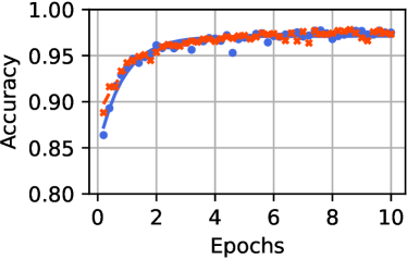
(a) MNIST, MLP

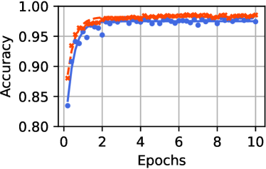
(b) MNIST, CNN

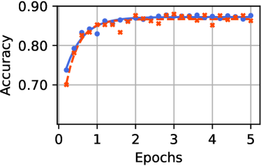
(c) AGNews, TextCNN

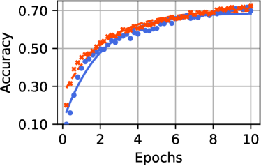
(d) CIFAR10, CNN

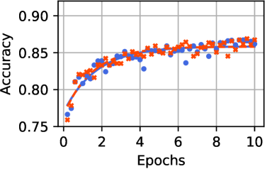
(e) CIFAR10, AlexNet

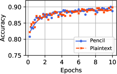
(f) CIFAR10, ResNet50

Figure 1: Test accuracies for trained models. (a) $\sim$ (d) are for models trained from scratch; (e) and (f) are for models trained via transfer learning.

We also report the total time and communication needed to train these NNs for one epoch in Table III. We measure the overheads for Pencil both with and without preprocessing optimization, denoted as Pencil and Pencil⁺ respectively. For the preprocessing phase, we set the number of masks to $m=8$. In the LAN network setting, Pencil without preprocessing can train CNNs for MNIST and CIFAR10 from scratch (10 epochs) within 7.8 hours and 280 hours, respectively. When the preprocessing technique is enabled, the training times are further reduced to 4.4 hours and 229 hours, respectively. In the WAN setting, we see a throughput reduction of $30\%\sim 50\%$, since the communication overhead is comparable to computation overhead. We observe that in training CNN for CIFAR10, the improvement of the preprocessing technique is not as significant as the previous 3 NNs. This is because a significant portion of training overhead of this NN is introduced by the non-linear evaluations (e.g., ReLU), while the preprocessing technique focuses on linear layers.

VI-C2 Transfer Learning Models

We now evaluate applying Pencil in transfer learning: MO uses a publicly available pre-trained model as the feature extractor, and subsequently trains a classifier on top of it. Since models pre-trained on large general datasets achieve robust feature extraction, transfer learning can significantly reduce the convergence time and improve test accuracy on specialized datasets, as shown by [46, 26]. Before training starts, both DO and MO obtain the public feature extractor. During training, the DO first passes its data through the feature extractor to get intermediate representations (IRs), and the classifier is trained privately on these IRs.

In our experiments, we use two publicly available pre-trained models, AlexNet [35] and ResNet50 [23] as the feature extractor. The complete models are denoted with the pre-trained model’s name (see Appendix -D for the detailed architecture). The results are shown in Table II and Figure 1. The best accuracy for CIFAR10 is improved to 90.02%, compared with the train-from-scratch CNN (71.69%). Meanwhile, the training time and communication overhead are also greatly reduced, as shown in Table III. For instance, transfer learning of ResNet50 sees a $4.4\times$ boost in throughput compared to training-from-scratch CNN, and can be trained within 6.2 hours in the LAN setting.

Key takeaways: for relatively large models like ResNet50 (with 25 million parameters), the overhead of cryptographic training from scratch is still significant. Augmented with transfer learning, cryptographic training can be more practical.

VI-C3 Training with Heterogeneous DOes

In this segment, we evaluate the extensibility of Pencil. We consider the case where the datasets owned by different DOes are biased, so it is desirable for the MO to incorporate the data from multiple DOes. In our experiment, we create five DOes, each with a dataset dominated by only two labels from the CIFAR10 dataset. For each training step, the MO trains the model with one of these DOes in turn. Finally MO tests the trained model with a test set with all ten labels. We evaluate with the two models used for CIFAR10. The results are shown in Figure 2. Clearly, in the case where the datasets owned by different DOes are highly heterogeneous, extending the training with more DOes is necessary to achieve high test accuracies.

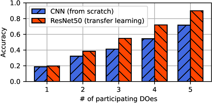
Figure 2: Test accuracies of the models trained with different numbers of heterogeneous DOes.

VI-C4 Impact of the DP Noises

In § III-B2, Pencil designs a secret-shared version of DPSGD algorithm to allow the DOes to add DP noises to the weight updates. In this part, we evaluate the impact of DP noises on model performance. We use the two models of CIFAR10 in this experiment. We first estimate the gradient bound $C$ used in our algorithm to be $8$, then we conduct the experiments with different noise levels $\sigma$, with a fixed batch size $B=64$. The models are trained for 10 epochs. The results are shown in Table IV. We observe that the accuracy slightly drops ($<2$%) given $\sigma\leq 10^{-2}$. In § VI-F, we empirically demonstrate that $\sigma=10^{-2}$ is sufficient to defend against the reconstruction attacks on the gradients.

$\sigma$	$(\epsilon,\delta)$-DP	Accuracy
		CNN	ResNet50
0	None	71.69%	90.02%
0.005	$(114,10^{-5})$	71.20%	89.71%
0.010	$(57,10^{-5})$	70.32%	89.29%
0.020	$(28.5,10^{-5})$	68.87%	88.47%
0.050	$(11.4,10^{-5})$	57.01%	85.17%

TABLE IV: Test accuracy of CIFAR10-CNN and ResNet50 trained with DP-mechanism of different noise levels $\sigma$.

VI-D Performance Breakdown

We present the performance breakdown of Pencil.

Linear Protocols. We inspect the time and communication overhead required to train a single linear layer in Pencil. The overhead of truncation is excluded. The results are shown in Table V. For training time, the preprocessing technique achieves $3\times\sim 5\times$ online speedup over the basic design. The communication cost is also reduced by $90\%$ for fully connected layers and $2/3$ for 2d-convolutional layers.

		Pencil		Pencil+
$n_{i}$	$n_{o}$	Time	Comm.	Time	Comm.
256	100	6.8ms	0.40MB	1.2ms	18KB
512	10	2.6ms	0.17MB	0.9ms	14KB
2048	1001	256.1ms	5.51MB	30.3ms	822KB

(a) Fully connected layers

				Pencil		Pencil+
$c_{i}$	$c_{o}$	$h,w$	$s$	Time	Comm.	Time	Comm.
64	64	$16^{2}$	5	165ms	3.61MB	13ms	0.75MB
3	64	$56^{2}$	3	244ms	11.61MB	100ms	4.71MB
64	3	$56^{2}$	3	237ms	11.51MB	86ms	4.80MB

(b) 2d-convolutional layers

TABLE V: Online training overheads of linear layers. Batch size is 64 and the results are averaged across samples. $n_{i}$ and $n_{o}$ denote the input and output neurons of a fully connected layer. $c_{i},c_{o}$ denote input and output channels of a convolutional layer. $h,w$ is input image size and $s$ is the kernel size.

Acceleration of Hardware Implementation. We further zoom into the performance of individual HE operators. In particular, we report the performance of our GPU-based BFV implementation and compare it with the state-of-the-art CPU implementation of Microsoft SEAL library [52]. For a complete comparison, we also implement the SIMD encoding/decoding functionality used in SEAL. The results are listed in Table VI. On average, our hardware implementation achieves $10\times$ acceleration over CPU implementation. We notice that there are other GPU acceleration works for HE (e.g., [60, 58]), but experimentally evaluating them is difficult since they are close-sourced.

HE Operation	GPU	CPU	Speedup
	(Ours)	([52])
Encoding	38	97	2.5$\times$
Decoding	65	114	1.8$\times$
Encryption	155	2611	16.8$\times$
Decryption	94	653	6.9$\times$
Addition	2	33	16.5$\times$
Multiplication	506	8362	16.5$\times$
Relinearization	38	173	4.6$\times$
Plain Mult.	178	1130	6.3$\times$
Rotation	366	1532	4.2$\times$

TABLE VI: Time overhead ($\mu$s) of various HE operations.

VI-E Efficiency Comparison with Prior Art

In this section, we compare the training efficiency of Pencil with prior art of MPC. As discussed in § I-B, machine learning protocols using MPC rely on the non-colluding assumption, unless the MO and DOes themselves participate as computing servers, which, unfortunately, has suffer from the extensibility problems for the 2/3/4-PC frameworks or scalability problem for general $n$-PC frameworks. Nevertheless, we compare the efficiency of Pencil with two MPC frameworks, QUOTIENT [3] and Semi2k [13]. The former is a non-extensible 2-PC framework, and the latter is extensible to any number of parties but we instantiate it with only 2 parties for maximum efficiency. The results are listed in Table VII. QUOTIENT does not provide communication costs in their paper, so we only compare its throughput. On average, Pencil without and with preprocessing optimization respectively achieves a speed-up of $13\times$ and $40\times$ over [3] and 2 orders of magnitude over [13].

	Throughput ($10^{4}$ img/h)				Comm. (MB/img)
Model	[3]	[13]	$\mathsf{P}$	$\mathsf{P}^{+}$	[13]	$\mathsf{P}$	$\mathsf{P}^{+}$
$2\times 128\mathsf{FC}$	0.7	0.11	9.7	29.3	552	1.7	0.2
$3\times 128\mathsf{FC}$	0.6	0.10	8.1	18.9	658	2.2	0.3
$2\times 512\mathsf{FC}$	0.2	0.03	2.6	13.2	3470	5.2	0.8

TABLE VII: Performance comparison with QUOTIENT [3] and Semi2k [13] in the 2 party setting. The models are represented as $n\times m\mathsf{FC}$, as used by [3]. $\mathsf{P}$ represents Pencil and $\mathsf{P}^{+}$ represents Pencil⁺.

For extensibility, we compare Pencil with [13] in the setting with over 2 parties on the MLP model of MNIST. The results are displayed in Table VIII. As a general $n$-PC architecture without the non-concluding assumption, the overhead of [13] grows significantly with more parties. In contrast, the overhead of Pencil remains the same regardless of the number of parties, because the multiparty training procedure is decomposed into 2-PC in every training step, and switching DOes between steps is cost-free.

	Throughput ($10^{3}$ img/h)			Comm. (per img)
Model	[13]	Pencil	Pencil+	[13]	Pencil	Pencil+
2 parties	1.11	97	265	0.55GB	1.7MB	0.2MB
3 parties	0.61	97	265	2.58GB	1.7MB	0.2MB
4 parties	0.41	97	265	6.06GB	1.7MB	0.2MB
5 parties	0.07	97	265	57.69GB	1.7MB	0.2MB

TABLE VIII: Performance comparison with Semi2k [13] in multiple party setting. The model is MNIST-MLP.

VI-F Pencil Against Attacks

Gradient Matching Attack [63] tries to reconstruct the original input using the model updates. Pencil proposes a secret-shared version of DPSGD to prevent this attack. In this segment, we evaluate the effectiveness of our method. We use the train-from-scratch CNN on CIFAR10 to conduct the evaluation. Note the attack requires a very small batch size, so we set the batch size to one. The reconstruction results are shown in Figure 3, together with the original input image data. It is clear that a noise level of $10^{-2}$ is sufficient to protect the original data. In practice, the training batch size is much larger (e.g., 64), which could further reduce the requirements of noise levels.

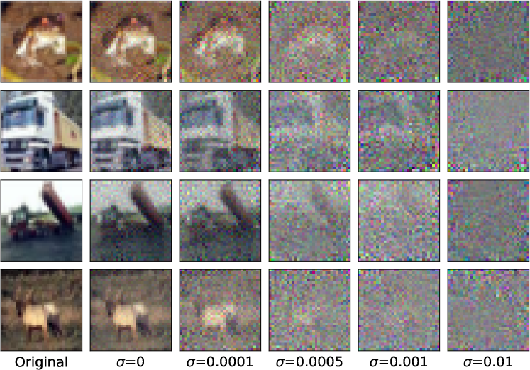
Figure 3: Gradient matching attack [63] defended with different levels of noise

In addition, the attacker may try to reduce the noise by introducing a regularization term into the optimization goal [20]. However, when the perturbations added to the gradients are large enough, such an attack would only produce smoothed but unidentifiable reconstructions. We defer the results in Appendix -E.

Adaptive Attacks against the Preprocessing Design. We further consider an adaptive attack against the preprocessing design in Pencil. In particular, a semi-honest MO may try to reconstruct the individual inputs from the linear combination of $\sum_{k\in[m^{\prime}]}a_{k}\mathbf{v}_{k}=\hat{\mathbf{v}}$ in Equation (9) (for simplicity, we let $n_{k}=k$).

Suppose MO tries to obtain one specific element $v_{i}$ in $\mathbf{v}_{i}$ (e.g., a specific pixel in an image). $v_{i}$ satisfy $\sum_{k\in[m^{\prime}]}a_{k}v_{k}=\hat{v}$. We launch the attack by the solving the problem stated in the proof sketch of Corollary IV.1 and list the difficulty of the attack for several different sets of $m,f$ in Table IX, with a comparison to RSA modulus length $k$ offering equivalent bit security [45].

We further empirically evaluate this attack on CIFAR10 dataset for a very small $m=2$ and precision $f=10$. MO presumes the pixel values of the normalized image are within $(-2,2)$. It takes around 62.1 seconds for MO (single-thread, using the CPU stated in § VI-B) to obtain one pixel correctly. Thus, by proper setting of $m$ and $f$, e.g., $m=8,f=25$, it would requires $9.5\times 10^{55}$ seconds (roughly $10^{48}$ years) to break one pixel. Symmetrically, it is equally difficult for a curious DO to derive the model parameters.

$m$	$f$	Search space	RSA-$k$	Time to Break
2	10	20 bits	$<512$	62.1 seconds
2	25	50 bits	$<512$	2114 years
4	25	100 bits	$\sim 2048$	$2.38\times 10^{18}$ years
8	25	200 bits	$\sim 7680$	$3.02\times 10^{48}$ years

TABLE IX: Hardness of the adaptive attack against the preprocessing optimization. RSA-$k$ means the RSA modulus bit length offering equivalent security guarantees. Time to break is evaluated or estimated using the CIFAR10 dataset.

VII Discussion and Future Work

VII-A Other Related Work

We cover the related work that is not discussed in § I-B.

Private Inference in Machine Learning. A series of art try to address the problem of private inference. In this setting, a client wishes to do inference on its private data on a third-party model deployed by a service provider. CryptoNets [17] and Gazelle [29] tackles this problem using the HE primitives. [17] uses the SIMD technique of BFV within the batch size dimension, thus requiring a huge batch size of 8192 to reach maximum throughput. [29] instead designs algorithms to exploit SIMD within one inference sample. It also combines garbled circuits (GC) for non-linear layers, while [17] changes non-linear layers to squaring function. On top of [29], Delphi [40] introduces a method to move all computationally heavy homomorphic operations to a preprocessing phase. However, this preprocessing must be executed once for every single sample on the fixed model weights. Thus, it is not applicable in training where the model weights are dynamic.

Recent developments of CrypTFlow2 [49] and Cheetah [25] adapts oblivious transfer (OT) to substitute GC to improve efficiency. Further, Cheetah [25] proposes to apply the polynomial homomorphism instead of the SIMD technique in HE for linear computation. We adopt polynomial encoding as a primitive in Pencil and adapt it for batched inputs in matrix multiplication and 2D convolution, similar to [22] and [38].

Hardware Acceleration in ML. Hardware acceleration has been widely applied in the field of machine learning. Mainstream ML frameworks all support GPU or TPU acceleration, but only for plaintext ML. Extending hardware acceleration to privacy-preserving learning is a less charted area. Recently, [30, 54] explores hardware acceleration for various MPC primitives, by moving various linear and non-linear operations onto GPU, under a setting of 3 or more servers. Some art further explores specialized FPGA or ASIC architecture. For instance, [64] accelerates the generation of multiplication triples using a trusted FPGA chip. There are also proposals to accelerate HE primitives. For instance, the widely used HE framework, Microsoft SEAL [52], supports multi-threading. [5] implements a simplified version of CKKS cryptosystem (without relinearization or rescaling) on GPU.

VII-B Limitations and Explorations

Parameter Selection. Private inference framework of Cheetah [25] uses BFV with $t=2^{41},q\approx 2^{109},f=12$, with multiplicative depth of only 1. However, Pencil need a much higher precision of $f=25$ bits to keep the gradients from diminishing into noises when training deep NNs. This also enforces a larger ciphertext modulus $q\approx 2^{180}$. Exploring a good balance between precision and HE parameters is an interesting direction. Recently, [48] proposed to use mixed bit-widths in different NN operators to control the precision at a smaller granularity, which may be adapted to our framework.

Gradient Clipping. In Pencil, to protect the privacy of model updates, DO cannot directly clip the gradients as the original DPSGD algorithm [2]. Instead, DO estimates an upper bound $C$ of gradients beforehand. Thus, the added DP noises may be slightly higher. A straightforward solution is to let MO compute the gradient norm in the encrypted domain and sends it to DO, which, however, imposes non-trivial overhead. We leave further exploration to future work.

VIII Conclusion

In this work, we present Pencil, a collaborative training framework that simultaneously achieves data privacy, model privacy, and extensibility of multiple data providers. Pencil designs end-to-end training protocols by combining HE and MPC primitives for high efficiency and utilizes a preprocessing technique to offload HE operations into an offline phase. Meanwhile, we develop a highly-parallelized GPU version of the BFV HE scheme to support Pencil. Evaluation results show that Pencil achieves training accuracy nearly identical to plaintext training, while the training overhead is greatly reduced compared to prior art. Furthermore, we demonstrate that Pencil is secure against both existing and adaptive attacks.

-A Polynomial encoding method

We briefly introduce the polynomial encoding method to evaluate $[\![\mathbf{y}]\!]=\mathbf{W}\circ[\![\mathbf{v}]\!]$ in the BFV scheme, for $\circ$ as matrix multiplication and 2d-convolution (i.e., $\mathsf{Conv2d}(\mathbf{v};\mathbf{W})$).

Matrix multiplication. We use an improved version of the polynomial encoding method from [25], as proposed by [22]. This improved version further takes the batch size dimension into account and reduces the communication costs for matrix multiplication.

Let weights be $\mathbf{W}\in\mathbb{Z}_{t}^{n_{o}\times n_{i}}$, and batched input be $\mathbf{v}\in\mathbb{Z}_{t}^{n_{i}\times B}$ (as $B$ column vectors). We assume $n_{o}n_{i}B\leq N$, the polynomial degree of the BFV scheme. Larger matrices could be partitioned into smaller blocks, and the evaluation could be done accordingly.

The input $\mathbf{v}=(v_{ij})_{i\in[n_{i}],j\in[B]}$ is encoded through $\pi_{v}$ as a polynomial

$$v=\pi_{v}(\mathbf{v})=\sum_{j=0}^{n_{i}-1}\sum_{k=0}^{B-1}v_{jk}x^{kn_{o}n_{i}+j}.$$

The weights $\mathbf{W}=(w_{ij})_{i\in[n_{o}],j\in[n_{i}]}$ are also encoded through $\pi_{W}$ as a polynomial (note how it is “reversely” encoded)

$$W=\pi_{W}(\mathbf{W})=\sum_{i=0}^{n_{o}-1}\sum_{j=0}^{n_{i}-1}W_{ij}x^{in_{i}+n_{i}-1-j}.$$

$v$ is encrypted in the BFV scheme, and the evaluator could evaluate the polynomial product $W\cdot[\![v]\!]$ in the encrypted domain, obtaining an encrypted polynomial $[\![y]\!]$, where $y=Wv$. After decryption, $y=\sum_{i=0}^{n_{o}n_{i}B-1}y_{i}x^{i}$ could be decoded through $\pi_{y}^{-1}$ to obtain the desired coefficients.

$$\mathbf{W}\cdot\mathbf{v}=\mathbf{y}=\pi_{y}^{-1}(y)=(y_{kn_{o}n_{i}+in_{i}+n_{i}-1})_{ik}$$

The correctness comes from the observation that the $(kn_{o}n_{i}+in_{i}+n_{i}-1)$-th term of $y$ is exactly

$$y_{kn_{o}n_{i}+in_{i}+n_{i}-1}=\sum_{j\in[n_{i}]}W_{ij}v_{jk}.$$

2D convolution. We also improve the method of [25] for 2D convolution to adapt the batched input. Specifically, similar to the idea for matrix multiplication, we consider the output channel dimension and the batch size dimension in the polynomial encoding primitive.

Let weights $\mathbf{W}\in\mathbb{Z}_{t}^{c_{o}\times c_{i}\times s\times s}$, batched input $\mathbf{v}\in\mathbb{Z}_{t}^{B\times c_{i}\times h\times w}$. For simplicity, we assume $Bc_{o}c_{i}hw\leq N$. Larger inputs or weights could be partitioned to meet this requirement.

The input $\mathbf{v}=(v_{b,c,i,j})_{b\in[B],c\in[c_{i}],i\in[h],j\in[w]}$ is encoded as a polynomial

$$v=\pi_{v}(\mathbf{v})=\sum_{b=0}^{B-1}\sum_{c=0}^{c_{i}-1}\sum_{i=0}^{h-1}\sum_{j=0}^{w-1}v_{b,c,i,j}x^{\mathsf{index}_{v}(b,c,i,j)}$$

$$\mathrm{where~{}}\mathsf{index}_{v}(b,c,i,j)=bc_{o}c_{i}hw+chw+iw+j.$$

The weights $\mathbf{W}=(W_{c^{\prime},c,i,j})_{c^{\prime}\in[c_{o}],c\in[c_{i}],i,j\in[h]}$ are also encoded reversely through $\pi_{W}$ as a polynomial

$$W=\pi_{W}(\mathbf{W})=\sum_{c^{\prime}=0}^{c_{o}-1}\sum_{c=0}^{c_{i}-1}\sum_{i=0}^{h-1}\sum_{j=0}^{w-1}W_{c^{\prime},c,i,j}x^{\mathsf{index}_{W}(c^{\prime},c,i,j)}$$

$$\mathrm{where~{}}\mathsf{index}_{W}(c^{\prime},c,i,j)=O+c^{\prime}c_{i}hw-chw-iw-j$$

$$\mathrm{and~{}}O=(c_{i}-1)hw+(s-1)w+s-1.$$

With this encoding, $[\![y]\!]=W\cdot[\![v]\!]$ has the desired result at the coefficients of specific terms. Precisely, if we denote $y=\sum_{i=0}^{Bc_{o}c_{i}hw-1}y_{i}x^{i}$, the decoding function is

$$\mathbf{y}=\pi_{y}^{-1}(y)=(y_{\mathsf{index}_{y}(b,c^{\prime},i,j)})_{b\in[B],c^{\prime}\in[c_{o}],i\in[h],j\in[w]}$$

$$\mathrm{where~{}}\mathsf{index}_{y}(b,c^{\prime},i,j)=bc_{o}c_{i}hw+O+c^{\prime}c_{i}hw+iw+j.$$

Therefore, after decrypting $[\![y]\!]$, one could obtain the complete result of $\mathbf{y}=\mathsf{Conv2d}(\mathbf{v};\mathbf{W})$.

-B Non-linear protocols

We briefly introduce the state-of-the-art ReLU, division (used in average pooling) and truncation protocols from prior art [49, 25] used in Pencil. These protocols are mostly based on oblivious transfers (OT)  [61]. In an $1$-out-of-$n$ oblivious transfer, there are two parties denoted as the Sender and the Receiver. The Sender provides $n$ messages while the Receiver takes $1$ of them, and Sender could not learn which one the Receiver takes while the Receiver could not learn any other messages except the chosen one.

ReLU. The ReLU activation function consists of a comparison protocol and a multiplexing (bit-injection) protocol.

$$\mathsf{ReLU}(x)=\mathsf{DReLU}(x)\cdot x=\mathbf{1}\{x\geq 0\}\cdot x$$

$\mathbf{1}\{x>0\}$ could be obtained from the most significant bit of the secret shared $x=\left\langle x\right\rangle_{0}+\left\langle x\right\rangle_{1}$, with

$$\mathbf{1}\{x\geq 0\}=\lnot\text{MSB}(x)$$

$$=\text{MSB}(\left\langle x\right\rangle_{0})\oplus\text{MSB}(\left\langle x\right\rangle_{1})\oplus\mathbf{1}\{2^{\ell-1}-\left\langle x\right\rangle_{0}<\left\langle x\right\rangle_{1}\}$$

The last term requires a secret comparison protocol where the two parties input $a=2^{\ell-1}-\left\langle x\right\rangle_{0}$ and $b=\left\langle x\right\rangle_{1}$ respectively. The secret comparison protocol is implemented with OT and bit-and protocol [49]. Specifically, the $\ell$-bit integer is decomposed into multiple blocks, each with $m$ bits. Then the two parties invokes 1-out-of-$2^{m}$ OT to obtain the greater-than and equality comparison results for each separate block. These comparison results of $\lceil\ell/m\rceil$ blocks are combined in a tree structure using a bit-and protocol (also implemented with OTs), according to the following observation:

$$\mathbf{1}\{a<b\}=\mathbf{1}\{a_{1}<b_{1}\}\oplus(\mathbf{1}\{a_{1}=b_{1}\}\land\mathbf{1}\{a_{0}<b_{0}\})$$

where $a=a_{1}||a_{0},b=b_{1}||b_{0}$. This observation indicates that the comparison result of larger bit-length integers could be obtained from their smaller bit-length blocks.

Finally, the multiplexing of ReLU is constructed with two OTs, where the two parties could select with their share of $\left\langle\mathsf{DReLU}(x)\right\rangle$, resulting in a canceling to zero when their selection bits are the same, and the original $x$ otherwise. This multiplexing protocol is detailed in Algorithm 6 of Appendix A in [49].

Division and Truncation. In average pooling, we need to use the division protocol where the shared integers are divided with a public divisor. In truncation, the shared integers are right-shifted $f$ bits. Our used neural networks only use average pooling of $2\times 2$ kernels. Therefore, the division used could also be considered a truncation of $2$ bits, and thus we only introduce the truncation protocol. Nevertheless, for the general case, the division protocol proposed by [49] (Algorithm 9 in Appendix D) could be used.

For truncation, SecureML [42] first proposed a protocol where each party directly performs local right-shift on its share. While lightweight, this protocol could introduce two kinds of errors: (1) a large error when the two shares’ addition wraps over the ring; (2) a small error on the least significant bit. For accurate truncation, [49] instead invokes secret comparison protocols to compute the error terms and correct both the small and the large error by adding a correction term. Recently, [25] observes that in private machine learning, as we are dealing with scaled decimals, the small 1-bit error would hardly affect the accuracies. Thus, [25] proposes an approximate truncation protocol that only handles the possible large error, greatly reducing the overheads.

-C Security proofs

We give the proof for Theorem IV.1.

• We describe the simulators for data privacy and model privacy below, after which we provide a full hybrid argument that relies on the simulators.

  Simulator Protocol for Data Privacy. The simulator $\mathsf{Sim}$, when provided with the MO’s view (including the model parameters $\mathbf{M}$, weight update $\nabla_{\mathbf{W}},\nabla_{\mathbf{b}}$ and shares $\langle\mathbf{X}\rangle_{0},\langle\nabla_{\mathbf{Y}}\rangle_{0}$ of each trainable linear layer in each training iteration), proceeds as follows:

  • $\mathsf{Sim}$ chooses an uniform random tape for the MO.

  • $\mathsf{Sim}$ chooses keys $\mathsf{pk},\mathsf{sk}$ for the HE scheme.

  • For every execution of Algorithm 1, instead of sending the encryption of its share $[\![\langle\mathbf{X}\rangle_{1}]\!]$, $\mathsf{Sim}$ simply sends encryption of a zero tensor $[\![\mathbf{0}]\!]$ (with the same shape as $\mathbf{X}$) to MO.

  • For every execution of Algorithm 2, similarly, $\mathsf{Sim}$ sends encryption of zeros instead of $[\![\langle\mathbf{X}\rangle_{1}]\!],[\![\langle\nabla_{\mathbf{Y}}\rangle_{1}]\!]$ to MO. Moreover, for $\widetilde{\nabla_{\mathbf{W}}}$, it sends $\nabla_{\mathbf{W}}-\mathbf{s}+\langle\nabla_{\mathbf{Y}}\rangle_{0}\circ\langle\mathbf{X}\rangle_{0}+\mathbf{e}$.

  • For non-linear layer evaluations, $\mathsf{Sim}$ uses randomized tensors as its share of the input.

Simulator Protocol for Model Privacy. The simulator $\mathsf{Sim}$, when provided with the DO’s view (including the dataset $\mathcal{D}$ and the shares $\langle\mathbf{X}\rangle_{1},\langle\nabla_{\mathbf{Y}}\rangle_{1}$ of each trainable layer in each training iteration), proceeds as follows:

• $\mathsf{Sim}$ chooses an uniform random tape for the DO.

• $\mathsf{Sim}$ receives $\mathsf{pk}$ of the HE scheme from the DO.

• For every execution of Algorithm 1, the $\mathsf{Sim}$ receives $[\![\langle\mathbf{X}\rangle_{1}]\!]$ but sends $[\![\langle\mathbf{Y}\rangle_{1}]\!]=[\![-\mathbf{s}]\!]$ back, for some random tensor $\mathbf{s}$.

• For every execution of Algorithm 2, similarly, the $\mathsf{Sim}$ sends only $[\![-\mathbf{s}]\!]$ back for decryption, instead of $[\![\nabla_{\mathbf{W}}^{\mathsf{cross}}-\mathbf{s}]\!]$.

• For non-linear layer evaluations, $\mathsf{Sim}$ uses randomized tensors as its share of the input.

Now we show that the two simulated distribution is indistinguishable from the real-world distribution.

Proof with a corrupted MO. We show that the real world distribution is computationally indistinguishable from the simulated distribution via a hybrid argument. In the final simulated distribution, the simulator does not use the DO’s dataset as input, and so a corrupted DO learns nothing in the real world.

• $\mathsf{Hyb}_{0}$: This corresponds to the real world distribution where the DO uses its training dataset $\mathcal{D}$.

• $\mathsf{Hyb}_{1}$: In this hybrid, we change the DO’s message in Algorithm 1. DO sends the homomorphic encryption of a zero tensor $[\![\mathbf{0}]\!]$ instead of sending $[\![\langle\mathbf{X}\rangle_{1}]\!]$. It follows from the property of the homomorphic encryption (ciphertexts are computationally indistinguishable) that $\mathsf{Hyb}_{1}$ is indistinguishable from $\mathsf{Hyb}_{0}$.

• $\mathsf{Hyb}_{2}$: In this hybrid, similarly we change DO’s message in Algorithm 2. DO again uses encryption of zeros to substitute $[\![\langle\mathbf{X}\rangle_{1}]\!]$, $[\![\nabla_{\mathbf{Y}}^{C}]\!]$. $\mathsf{Hyb}_{2}$ is indistinguishable from $\mathsf{Hyb}_{1}$.

• $\mathsf{Hyb}_{3}$: In this hybrid, we further change DO’s behavior in Algorithm 2: with the knowledge of MO’s view, DO sends $\nabla_{\mathbf{W}}-\mathbf{s}+\langle\nabla_{\mathbf{Y}}\rangle_{0}\odot\langle\mathbf{X}\rangle_{0}+\mathbf{e}$ as $\widetilde{\nabla_{\mathbf{W}}}$. Since this message exactly allows the MO to obtain $\nabla_{\mathbf{W}}$, thus $\mathsf{Hyb}_{3}$ is indistinguishable from $\mathsf{Hyb}_{2}$.

• $\mathsf{Hyb}_{4}$: In this hybrid, we replace DO’s inputs to the non-linear evaluation by random tensors. It follows from the security of these non-linear evaluation MPC protocols [25, 49], that $\mathsf{Hyb}_{4}$ is indistinguishable from $\mathsf{Hyb}_{3}$, completing the proof.

Proof with a corrupted DO. We show that the real-world distribution is computationally indistinguishable from the simulated distribution via a hybrid argument. In the final simulated distribution, the simulator does not use the MO’s model weights $\mathbf{M}$ for training, and so a corrupted DO learns nothing in the real world.

• $\mathsf{Hyb}_{0}$: This corresponds to the real world distribution where the MO uses its model weights $\mathbf{M}$.

• $\mathsf{Hyb}_{1}$: In this hybrid, we change the MO’s behavior in Algorithm 1. Instead of using the weights $\mathbf{W}$ to calculate $\mathbf{W}\circ[\![\mathbf{X}]\!]-\mathbf{s}$, MO simply samples $\mathbf{s}$ and sends back $[\![-\mathbf{s}]\!]$. Also, MO does not add bias term $\mathbf{b}$ to its share of output $\mathbf{Y}$. It follows from the security of homomorphic encryption that $\mathsf{Hyb}_{1}$ is computationally indistinguishable from $\mathsf{Hyb}_{0}$.

• $\mathsf{Hyb}_{2}$: In this hybrid, similarly we change the MO’s behavior in Algorithm 2 by substituting the ciphertext message $[\![\nabla_{\mathbf{W}}^{\mathsf{cross}}-\mathbf{s}]\!]$ with simply $[\![-\mathbf{s}]\!]$. $\mathsf{Hyb}_{2}$ is computationally indistinguishable from $\mathsf{Hyb}_{1}$.

• $\mathsf{Hyb}_{3}$: In this hybrid, we replace MO’s inputs to the non-linear evaluation by random tensors. It follows from the security of these non-linear evaluation MPC protocols [25, 49], that $\mathsf{Hyb}_{3}$ is indistinguishable from $\mathsf{Hyb}_{2}$, completing the proof.

∎

-D Neural Network Architecture

Figure 4: MLP for the MNIST task [41, 47, 3]

Figure 5: CNN for the MNIST task [50]

Figure 6: TextCNN for the AGNews task [62]

Figure 7: CNN for the CIFAR10 task [56]

Figure 8: Transfer learning models for the CIFAR10 task

The neural networks used for the evaluation are listed in Figure 4, 5, 6, 7, 8. The neurons are the number of output dimensions for fully connected layers. The channels are the number of output channels for 2D convolution layers. For concision, the activation function ReLU is written directly after linear layers. The 1D convolution and 1D average pooling are implemented simply as a specialization of 2D variants.

-E Inverting Gradients

In this section we evaluate the gradient inverting attack introduced by [20], which introduces a regularization term to remove the noises in the reconstruction results. We again use CNN and CIFAR10 for evaluating this attack. The results are shown in Figure 9. The results confirm that, when $\sigma\geq 10^{-2}$ the reconstructed images are smoothed but completely unidentifiable.

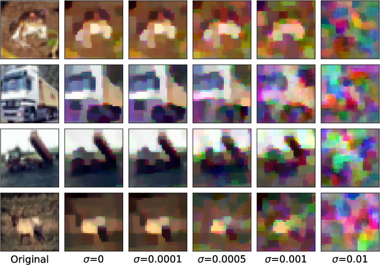
Figure 9: Gradient inverting attack [20] defended with different levels of noise

Appendix A Artifact Appendix

A-A Description & Requirements

A-A1 How to access

• DOI: https://doi.org/10.5281/zenodo.10140580

• GitHub: https://github.com/lightbulb128/Pencil

A-A2 Hardware dependencies

A computer with CUDA supporting GPU devices. The code has been tested on a machine with a NVIDIA RTX A6000 GPU and CUDA 11.7.

A-A3 Software dependencies

A Linux machine, with python $\geq$ 3.8 and CUDA $\geq$ 11.7. The code has been tested on Ubuntu 20.04.3 LTS.

A-A4 Benchmarks

MNIST, CIFAR10, AGNews datasets and pretrained ResNet50 and GPT-2 models are used. They are available from the torchvision, torchtext and transformers package.

A-B Artifact Installation & Configuration

The installation can be done via running build_dependencies.sh provided in the repository. At a high level, it clones the three dependencies (OpenCheetah, EzPC, seal-cuda) and builds them. OpenCheetah, EzPC are 2-party secure computation libraries providing non-linearities evaluation, which are adapted to provide python interfaces, and seal-cuda is a homomorphic encryption library with GPU parallelization providing linearities related utilities.

A-C Major Claims

• (C1): Models trained privately with Pencil has similar accuracy metrics as trained in plaintext, as shown by Table II and Fig. 1. Reproduced by Experiment (E1).

• (C2): Training costs in Pencil are acceptable as shown by Table III. Reproduced by Experiment (E2).

• (C3): Including more DOes with heterogeneous data could improve model accuracy in Pencil, as shown by Fig. 2. Reproduced by Experiment (E3).

• (C4): One could integrate DP methods to provide stronger privacy guarantees over the model gradients, as shown by Table IV. Reproduced by Experiment (E4).

A-D Evaluation

The evaluation mainly focuses on two parts: model accuracy and training cost. In the provided repository, gen_scripts.sh could be used to generate a series of evaluation scripts. These scripts are prefixed with fullhe or prep, corresponding to Pencil or Pencil⁺. Recall that Pencil uses online homomorphic encryption while Pencil⁺ uses the preprocessing optimization which conveys all HE computations to the offline phase. Each script itself simulates the two participants DO and MO, which communicate through a localhost port.

Each script represents a single experiment, either (1) to train a model and tests its accuracy, or (2) to measure the training cost of a single training step. The scripts will output logs in the corresponding logs/ folder with the same name as the script, which will contain the accuracy and cost measurement results.

A-D1 Experiment (E0)

[trivial.sh] Train the simplest model on MNIST for 1 epoch. This is used for checking whether the installation is functional. Estimated time: 0.6 and 0.2 hours for Pencil and Pencil⁺ respectively

A-D2 Experiment (E1)

[train_nn*.sh] Train the model end-to-end and outputs the accuracy every 1/5 epochs. Estimated times are listed in Table X.

A-D3 Experiment (E2)

[costs_nn*.sh] Train the model for one step and output the time and communication costs. For Pencil, cost evaluation time is expected to be below 1 minutes for each model. For Pencil⁺, the time also includes the preprocessing phase time, listed in Table III in the main paper for each model.

A-D4 Experiment (E3)

[dp*_nn*.sh] Train the model with different DP noise levels. Estimated times are listed in Table X.

A-D5 Experiment (E4)

[hetero_nn*.sh] Train the model with 5 simulated DOes with different data distributions. Estimated times are listed in Table X.

The end-to-end online training time for each NN listed in Table X could also be calculated from the throughput listed in the paper.

Task	Model	Pencil	Pencil+
MNIST	MLP	6.2	2.3
MNIST	CNN	7.8	4.4
AGNews	TextCNN	162	78.9
CIFAR10	CNN	278	227
CIFAR10	AlexNet	96	33.3
CIFAR10	ResNet50	27.3	6.5

TABLE X: Online training time (hours) for each model.

A-E Customization

The provided code could be run with other arguments than listed in the generated scripts, including learning rate, optimizer type, gradient clipping bounds and noise levels, etc.. The detailed list and usage are provided in the readme.md file in the repository.

References

- [1] “Complete guide to GDPR compliance,” Feb 2020, accessed: Nov. 2023. [Online]. Available: https://gdpr.eu/
- [2] M. Abadi, A. Chu, I. Goodfellow, H. B. McMahan, I. Mironov, K. Talwar, and L. Zhang, “Deep Learning with Differential Privacy,” in Proceedings of the 2016 ACM SIGSAC Conference on Computer and Communications Security (CCS), 2016.
- [3] N. Agrawal, A. Shahin Shamsabadi, M. J. Kusner, and A. Gascón, “QUOTIENT: Two-Party Secure Neural Network Training and Prediction,” in Proceedings of the 2019 ACM SIGSAC Conference on Computer and Communications Security (CCS), 2019.
- [4] F. am Main, “Enhancing cooperation in the fight against money laundering,” May 2022, accessed: Nov. 2023.
- [5] A. A. Badawi, L. Hoang, C. F. Mun, K. Laine, and K. M. M. Aung, “PrivFT: Private and Fast Text Classification With Homomorphic Encryption,” IEEE Access, 2020.
- [6] J. C. Bajard, J. Eynard, M. Hasan, and V. Zucca, “A Full RNS Variant of FV Like Somewhat Homomorphic Encryption Schemes,” 2017.
- [7] D. Beaver, “Efficient multiparty protocols using circuit randomization,” in Advances in Cryptology (CRYPTO’91), 1992.
- [8] J. Blömer, R. Karp, and E. Welzl, “The rank of sparse random matrices over finite fields,” Random Structures & Algorithms, 1997.
- [9] K. Bonawitz, H. Eichner, W. Grieskamp, D. Huba, A. Ingerman, V. Ivanov, C. Kiddon, J. Konečný, S. Mazzocchi, B. McMahan, T. Van Overveldt, D. Petrou, D. Ramage, and J. Roselander, “Towards Federated Learning at Scale: System Design,” in Proceedings of Machine Learning and Systems, 2019.
- [10] K. Bonawitz, V. Ivanov, B. Kreuter, A. Marcedone, H. B. McMahan, S. Patel, D. Ramage, A. Segal, and K. Seth, “Practical Secure Aggregation for Privacy-Preserving Machine Learning,” in Proceedings of the 2017 ACM SIGSAC Conference on Computer and Communications Security (CCS), 2017.
- [11] H. Chaudhari, R. Rachuri, and A. Suresh, “Trident: Efficient 4PC Framework for Privacy Preserving Machine Learning,” in Proceedings 2020 Network and Distributed System Security Symposium, 2020.
- [12] C. Cooper, “On the Distribution of Rank of a Random Matrix over a Finite Field,” Random Struct. Algorithms, 2000.
- [13] R. Cramer, I. Damgård, D. Escudero, P. Scholl, and C. Xing, “Spd: Efficient mpc mod for dishonest majority,” in Advances in Cryptology (CRYPTO 2018), H. Shacham and A. Boldyreva, Eds., 2018.
- [14] A. Dalskov, D. Escudero, and M. Keller, “Fantastic four:Honest-MajorityFour-Party secure computation with malicious security,” in 30th USENIX Security Symposium (USENIX Security), 2021.
- [15] I. Damgård, D. E. Escudero, T. K. Frederiksen, M. Keller, P. Scholl, and N. Volgushev, “New Primitives for Actively-Secure MPC over Rings with Applications to Private Machine Learning,” 2019 IEEE Symposium on Security and Privacy (SP), 2019.
- [16] J. Deng, W. Dong, R. Socher, L.-J. Li, K. Li, and L. Fei-Fei, “ImageNet: A large-scale hierarchical image database,” in 2009 IEEE Conference on Computer Vision and Pattern Recognition, 2009.
- [17] N. Dowlin, R. Gilad-Bachrach, K. Laine, K. Lauter, M. Naehrig, and J. Wernsing, “CryptoNets: Applying Neural Networks to Encrypted Data with High Throughput and Accuracy,” in Proceedings of the 33rd International Conference on International Conference on Machine Learning (ICML), 2016.
- [18] J. Fan and F. Vercauteren, “Somewhat Practical Fully Homomorphic Encryption,” IACR Cryptol. ePrint Arch., vol. 2012, p. 144, 2012.
- [19] Y. Gao, M. Kim, S. Abuadbba, Y. Kim, C. Thapa, K. Kim, S. A. Camtep, H. Kim, and S. Nepal, “End-to-End Evaluation of Federated Learning and Split Learning for Internet of Things,” in 2020 International Symposium on Reliable Distributed Systems (SRDS), 2020.
- [20] J. Geiping, H. Bauermeister, H. Dröge, and M. Moeller, “Inverting Gradients - How Easy is It to Break Privacy in Federated Learning?” in Proceedings of the 34th International Conference on Neural Information Processing Systems (NIPS), 2020.
- [21] O. Gupta and R. Raskar, “Distributed learning of deep neural network over multiple agents,” J. Netw. Comput. Appl., 2018.
- [22] M. Hao, H. Li, H. Chen, P. Xing, G. Xu, and T. Zhang, “Iron: Private Inference on Transformers,” in Advances in Neural Information Processing Systems, 2022.
- [23] K. He, X. Zhang, S. Ren, and J. Sun, “Deep Residual Learning for Image Recognition,” in 2016 IEEE Conference on Computer Vision and Pattern Recognition (CVPR), 2016.
- [24] E. Hesamifard, H. Takabi, M. Ghasemi, and R. N. Wright, “Privacy-preserving Machine Learning as a Service,” Proceedings on Privacy Enhancing Technologies, 2018.
- [25] Z. Huang, W. jie Lu, C. Hong, and J. Ding, “Cheetah: Lean and fast secure Two-Party deep neural network inference,” in 31st USENIX Security Symposium (USENIX Security 22), 2022.
- [26] M. Huh, P. Agrawal, and A. Efros, “What makes ImageNet good for transfer learning?” 2016.
- [27] W. Jakob, J. Rhinelander, and D. Moldovan, “pybind11 – Seamless operability between C++11 and Python,” 2021, https://github.com/pybind/pybind11.
- [28] J. Jeon and J. Kim, “Privacy-Sensitive Parallel Split Learning,” in 2020 International Conference on Information Networking (ICOIN), 2020.
- [29] C. Juvekar, V. Vaikuntanathan, and A. Chandrakasan, “GAZELLE: A low latency framework for secure neural network inference,” in 27th USENIX Security Symposium (USENIX Security 18), 2018.
- [30] B. Knott, S. Venkataraman, A. Hannun, S. Sengupta, M. Ibrahim, and L. van der Maaten, “CrypTen: Secure Multi-Party Computation Meets Machine Learning,” in Advances in Neural Information Processing Systems, 2021.
- [31] V. Kolesnikov and R. Kumaresan, “Improved OT Extension for Transferring Short Secrets,” in Annual International Cryptology Conference, 2013.
- [32] J. Konecný, H. B. McMahan, F. X. Yu, P. Richtárik, A. T. Suresh, and D. Bacon, “Federated Learning: Strategies for Improving Communication Efficiency,” ArXiv, 2016.
- [33] N. Koti, A. Patra, R. Rachuri, and A. Suresh, “Tetrad: Actively Secure 4PC for Secure Training and Inference,” ArXiv, 2021.
- [34] A. Krizhevsky, “Learning Multiple Layers of Features from Tiny Images,” 2009.
- [35] A. Krizhevsky, I. Sutskever, and G. E. Hinton, “ImageNet Classification with Deep Convolutional Neural Networks,” Commun. ACM, 2017.
- [36] Y. Lecun, L. Bottou, Y. Bengio, and P. Haffner, “Gradient-based learning applied to document recognition,” Proceedings of the IEEE, 1998.
- [37] Q. Li, Z. Liu, Q. Li, and K. Xu, “martFL: Enabling Utility-Driven Data Marketplace with a Robust and Verifiable Federated Learning Architecture,” in Proceedings of the 2023 ACM SIGSAC Conference on Computer and Communications Security (CCS), 2023.
- [38] X. Liu and Z. Liu, “LLMs Can Understand Encrypted Prompt: Towards Privacy-Computing Friendly Transformers,” 2023.
- [39] H. B. McMahan, E. Moore, D. Ramage, S. Hampson, and B. A. y Arcas, “Communication-Efficient Learning of Deep Networks from Decentralized Data,” in International Conference on Artificial Intelligence and Statistics, 2016.
- [40] P. Mishra, R. Lehmkuhl, A. Srinivasan, W. Zheng, and R. A. Popa, “Delphi: A Cryptographic Inference System for Neural Networks,” in Proceedings of the 2020 Workshop on Privacy-Preserving Machine Learning in Practice, 2020.
- [41] P. Mohassel and P. Rindal, “ABY3: A Mixed Protocol Framework for Machine Learning,” Proceedings of the 2018 ACM SIGSAC Conference on Computer and Communications Security, 2018.
- [42] P. Mohassel and Y. Zhang, “SecureML: A System for Scalable Privacy-Preserving Machine Learning,” in 2017 IEEE Symposium on Security and Privacy (SP), 2017.
- [43] K. Nandakumar, N. Ratha, S. Pankanti, and S. Halevi, “Towards Deep Neural Network Training on Encrypted Data,” in 2019 IEEE/CVF Conference on Computer Vision and Pattern Recognition Workshops (CVPRW), 2019.
- [44] L. L. Ng and S. M. Chow, “SoK: Cryptographic Neural-Network Computation,” in 2023 IEEE Symposium on Security and Privacy (SP), 2023.
- [45] N. I. of Standards and Technology, “Security Requirements for Cryptographic Modules,” U.S. Department of Commerce, Washington, D.C., Tech. Rep. Special Publication 800-57 Part 1 Rev. 5, 2020.
- [46] M. Oquab, L. Bottou, I. Laptev, and J. Sivic, “Learning and Transferring Mid-level Image Representations Using Convolutional Neural Networks,” in 2014 IEEE Conference on Computer Vision and Pattern Recognition, 2014.
- [47] A. Patra and A. Suresh, “BLAZE: Blazing Fast Privacy-Preserving Machine Learning,” IACR Cryptol. ePrint Arch., p. 42, 2020.
- [48] D. Rathee, M. Rathee, R. K. Kiran Goli, D. Gupta, R. Sharma, N. Chandran, and A. Rastogi, “SiRnn: A Math Library for Secure RNN Inference,” in 2021 IEEE Symposium on Security and Privacy (SP), 2021.
- [49] D. Rathee, M. Rathee, N. Kumar, N. Chandran, D. Gupta, A. Rastogi, and R. Sharma, “CrypTFlow2: Practical 2-Party Secure Inference,” in Proceedings of the 2020 ACM SIGSAC Conference on Computer and Communications Security (CCS), 2020.
- [50] M. S. Riazi, C. Weinert, O. Tkachenko, E. M. Songhori, T. Schneider, and F. Koushanfar, “Chameleon: A Hybrid Secure Computation Framework for Machine Learning Applications,” in Proceedings of the 2018 on Asia Conference on Computer and Communications Security (ASIACCS), 2018.
- [51] S. Sav, A. Pyrgelis, J. R. Troncoso-Pastoriza, D. Froelicher, J.-P. Bossuat, J. Sousa, and J.-P. Hubaux, “POSEIDON: Privacy-Preserving Federated Neural Network Learning,” 2021.
- [52] “Microsoft SEAL (release 4.0),” https://github.com/Microsoft/SEAL, Mar. 2022, microsoft Research, Redmond, WA.
- [53] R. Shokri, M. Stronati, C. Song, and V. Shmatikov, “Membership Inference Attacks Against Machine Learning Models,” in 2017 IEEE Symposium on Security and Privacy (SP), 2017.
- [54] S. Tan, B. Knott, Y. Tian, and D. J. Wu, “CryptGPU: Fast Privacy-Preserving Machine Learning on the GPU,” in 2021 IEEE Symposium on Security and Privacy (SP), 2021.
- [55] C. D. D. Teran, “Collaboration Is Key in the Fight Against Anti-Money Laundering,” Feb 2023, accessed: Nov. 2023.
- [56] H. Tian, C. Zeng, Z. Ren, D. Chai, J. Zhang, K. Chen, and Q. Yang, “Sphinx: Enabling Privacy-Preserving Online Learning over the Cloud,” in 2022 IEEE Symposium on Security and Privacy (SP), 2022.
- [57] F. Tramèr, F. Zhang, A. Juels, M. K. Reiter, and T. Ristenpart, “Stealing machine learning models via prediction APIs,” in 25th USENIX security symposium (USENIX Security 16), 2016.
- [58] E. R. Türkoğlu, A. c. Özcan, C. Ayduman, A. C. Mert, E. Öztürk, and E. Savaş, “An Accelerated GPU Library for Homomorphic Encryption Operations of BFV Scheme,” in 2022 IEEE International Symposium on Circuits and Systems (ISCAS), 2022.
- [59] S. Wagh, D. Gupta, and N. Chandran, “SecureNN: 3-Party Secure Computation for Neural Network Training,” Proceedings on Privacy Enhancing Technologies, vol. 2019, 2019.
- [60] W. Wang, Z. Chen, and X. Huang, “Accelerating leveled fully homomorphic encryption using GPU,” in 2014 IEEE International Symposium on Circuits and Systems (ISCAS), 2014.
- [61] K. Yang, C. Weng, X. Lan, J. Zhang, and X. Wang, “Ferret: Fast Extension for Correlated OT with Small Communication,” in Proceedings of the 2020 ACM SIGSAC Conference on Computer and Communications Security (CCS), 2020.
- [62] X. Zhang, J. Zhao, and Y. LeCun, “Character-level Convolutional Networks for Text Classification,” in Advances in Neural Information Processing Systems, 2015.
- [63] B. Zhao, K. R. Mopuri, and H. Bilen, “iDLG: Improved Deep Leakage from Gradients,” 2020.
- [64] X. Zhou, Z. Xu, C. Wang, and M. Gao, “PPMLAC: High Performance Chipset Architecture for Secure Multi-Party Computation.” Association for Computing Machinery, 2022.
- [65] L. Zhu, Z. Liu, and S. Han, “Deep Leakage from Gradients,” in Advances in Neural Information Processing Systems. Curran Associates, Inc., 2019.