Angular Momentum Memory Effect

Abstract

Utilizing recent mathematical advances in proving stability of Minkowski spacetime with minimal decay rates and nonlinear stability of Kerr black holes with small angular momentum, we investigate the detailed asymptotic behaviors of gravitational waves generated in these spacetimes. Here we report and propose a new angular momentum memory effect along future null infinity. This accompanies Christodoulou’s nonlinear displacement memory effect and the spin memory effect. The connections and differences to these effects are also addressed.

Introduction.—Rapid progress has been made in the hyperbolic theory of mathematical general relativity. In particular, Kerr nonlinear stability with small angular momentum has been recently proven by Klainerman-Szeftel, Giorgi-Klainerman-Szeftel and the third author in the series of works KS:Kerr1 ; KS:Kerr2 ; KS:main ; GKS ; Shen . In addition, the global stability of Minkowski spacetime, first revealed by Christodoulou-Klainerman Ch-Kl , has been reproved under minimal decay assumptions of initial data by the third author Shenglobal . Detailed explicit hyperbolic estimates have been provided. With these, we revisit the field of memory effects of gravitational waves. In particular, in this article, we extend Christodoulou’s displacement memory Ch and Bieri’s extension BieriMemory to broader settings. Employing the newly defined intrinsic angular momentum introduced by Klainerman-Szeftel in KS:Kerr2 , we identify a new angular momentum memory effect. Links and differences to the spin memory effect PSZ are also discussed. In a later section, we also translate our results into Newman-Penrose (NP) formalism.

Preliminaries.—In a $3+1$ dimensional Lorentzian manifold $(\mathcal{M},{\bf g})$, we study the Einstein vacuum equations:

$$\operatorname{{\bf Ric}}_{\mu\nu}({\bf g})=0\quad\mbox{with}\quad\mu,\nu\in\{1,2,3,4\}.$$ (1)

We foliate the spacetime $\mathcal{M}$ by maximal hypersurfaces $\Sigma_{t}$ as level sets of a time function $t$ and by outgoing null cones $C_{u}$ as level sets of an optical function $u$. The intersections of $\Sigma_{t}$ and $C_{u}$ are 2-spheres denoted by $S(t,u)$ with $u\in\mathbb{R},t\geq 0$. We define the area radius of $S(t,u)$ by $r:=\sqrt{{|S(t,u)|}/{4\pi}}$. Let $T$ be the future-oriented unit vector normal to $\Sigma_{t}$, and $N$ be the outward unit normal vector of $S(t,u)$ that is tangential to $\Sigma_{t}$. With $T$ and $N$, we set the associated null frame to be $(e_{1},e_{2},e_{3},e_{4})$. Here $(e_{4},e_{3}):=(T+N,T-N)$ and $(e_{1},e_{2})$ is an orthonormal frame on $S(t,u)$. With $A,B\in\{1,2\}$ and ${\bf D}$ being the covariant derivative, we further introduce the null decomposition of the Ricci coefficients.

$${\underline{\chi}}_{AB} :={\bf g}({\bf D}_{A}e_{3},e_{B}),\qquad\quad\;\chi_{AB}:={\bf g}({\bf D}_{A}e_{4},e_{B}),$$

$$\operatorname{tr}{\underline{\chi}} :=\delta^{AB}{\underline{\chi}}_{AB},\qquad\qquad\;\;\;\;{\widehat{{\underline{\chi}}}}_{AB}:={\underline{\chi}}_{AB}-\frac{1}{2}\operatorname{tr}{\underline{\chi}}\,{\bf g}_{AB},$$

$$\operatorname{tr}\chi :=\delta^{AB}\chi_{AB},\qquad\qquad\;\;\;\;{\widehat{\chi}}_{AB}:=\chi_{AB}-\frac{1}{2}\operatorname{tr}\chi\,{\bf g}_{AB},$$

$${\underline{\omega}} :=\frac{1}{4}{\bf g}({\bf D}_{3}e_{3},e_{4}),\qquad\quad\,\,\,\;\,\;\omega:=\frac{1}{4}{\bf g}({\bf D}_{4}e_{4},e_{3}),$$

$${\underline{\eta}}_{A} :=\frac{1}{2}{\bf g}({\bf D}_{4}e_{3},e_{A}),\qquad\quad\;\;\eta_{A}:=\frac{1}{2}{\bf g}({\bf D}_{3}e_{4},e_{A}),$$

$$\zeta_{A} :=\frac{1}{2}{\bf g}({\bf D}_{e_{A}}e_{4},e_{3}),\qquad\quad\,{\underline{\xi}}_{A}:=\frac{1}{2}{\bf g}({\bf D}_{3}e_{3},e_{A}),$$

and curvature components

$$\alpha_{AB} :=\mathbf{R}(e_{A},e_{4},e_{B},e_{4}),\quad\;\;\,\underline{\alpha}_{AB}:=\mathbf{R}(e_{A},e_{3},e_{B},e_{3}),$$

$$\beta_{A} :=\frac{1}{2}\mathbf{R}(e_{A},e_{4},e_{3},e_{4}),\;\;\quad\;\underline{\beta}_{A}:=\frac{1}{2}\mathbf{R}(e_{A},e_{3},e_{3},e_{4}),$$

$$\rho :=\frac{1}{4}\mathbf{R}(e_{3},e_{4},e_{3},e_{4}),\quad\;\;\;\;\;\;\sigma:=\frac{1}{4}{{}^{*}\mathbf{R}}(e_{3},e_{4},e_{3},e_{4}),$$

where ${}^{*}\mathbf{R}$ denotes the Hodge dual of Riemann tensor $\mathbf{R}$. We also denote $\nabla$ as the induced covariant derivative on $S(t,u)$ and let $\nabla_{3}\psi$ and $\nabla_{4}\psi$ represent the projections of ${\bf D}_{3}\psi$ and ${\bf D}_{4}\psi$ to $S(t,u)$.

We remark that the final angular momentum $a_{f}$ and final mass $m_{f}$ of the spacetime are determined by taking the limit of geometrically constructed parameters associated to a family of finite admissible General Covariant Modulated (GCM) spacetimes. This construction is anchored on a GCM sphere $S_{*}$. Klainerman-Szeftel KS:Kerr2 introduced the associated angular momentum of $S_{*}$ as

$$J:=r^{5}(\operatorname{curl}\beta)_{\ell=1}.$$ (2)

Here $(\cdot)_{\ell=1}$ denotes the projection onto $\ell=1$ modes on the sphere. In their proof of Kerr stability, the definition of $J$ and its evolution play a crucial role. The intrinsic geometry of $S_{*}$ is uniquely determined by the uniformization theorem and its extrinsic properties are fixed by GCM conditions. For other definitions of angular momentum, interested readers are referred to CWY ; CWWY ; Rizzi .

Stability of Minkowski—The global nonlinear stability of Minkowski spacetime for the Einstein vacuum equations has been first established by Christodoulou-Klainerman Ch-Kl in 1993. In 2007, Bieri Bieri provided an important extension that requires one less derivative and weaker decay requirement for initial data compared to Ch-Kl . In Shenglobal , the third author extended the results of Bieri to minimal decay assumptions, as stated in Theorem 1 below. The proofs presented in Ch-Kl ; Bieri ; Shenglobal are based on the maximal-null foliation. In 2003, Klainerman-Nicolò Kl-Ni ; knpeeling revisited Minkowski stability in the exterior region of an outgoing null cone using the double null foliation. Later on, the third author ShenMink reproved the stability of Minkowski in this exterior region with more general initial data. For the latest updates and more related details about stability of Minkowski, interested readers are referred to ShenMink ; Shenglobal and references therein.

Theorem 1 (Global stability of Minkowski Shenglobal ).

Let $s\in(1,2]$ and consider a $s$–asymptotically flat initial data set $(\Sigma_{0},g,k)$, i.e.,

$$g_{ij}=\delta_{ij}+o(r^{-\frac{s-1}{2}}),\quad k_{ij}=o(r^{-\frac{s+1}{2}}),\quad i,j\in\{1,2,3\}.$$

Then, the nonlinear stability of Minkowski holds true in the future of $\Sigma_{0}$. Moreover, we have the following asymptotic behaviors in the exterior region:

$$\Gamma_{g}=O(r^{-\frac{s+1}{2}}),\qquad\Gamma_{b},\,\Gamma_{w},\,u\underline{\alpha}=O(r^{-1}|u|^{-\frac{s-1}{2}}),$$

where

$$\Gamma_{g} :=\left\{r\nabla\operatorname{tr}\chi,\,r\nabla\operatorname{tr}{\underline{\chi}},\,{\widehat{\chi}},\,\omega,\,{\underline{\omega}},\,\zeta,\,{\underline{\eta}},\,r\alpha,\,r\beta,\,r\rho,\,r\sigma\right\},$$

$$\Gamma_{b} :=\left\{\eta,\,\operatorname{tr}\chi-\frac{2}{r},\,\operatorname{tr}{\underline{\chi}}+\frac{2}{r},\,{\underline{\xi}}\right\},\qquad\;\Gamma_{w}:=\left\{{\widehat{{\underline{\chi}}}},\,r\underline{\beta}\right\}.$$

In this paper, we report that we can improve estimates in Theorem 1 as below. These improvements of the extra decay rates in $r$ enable us to demonstrate the weighted asymptotic limits of various geometric quantities. In particular, with these limits, we establish the formula for the angular momentum memory effect.

Lemma 2.

Under the same assumptions as in Theorem 1, we have the following improved decay estimates

$$\Gamma_{b} =O(r^{-\frac{s+1}{2}}),$$ (3)

$$\Gamma_{r} =O(r^{-2}|u|^{\frac{3-s}{2}}),\qquad\beta=O(r^{-4}|u|^{\frac{5-s}{2}}),$$ (4)

where $\Gamma_{r}:=\Gamma_{g}\cup\Gamma_{b}\setminus\{\eta,\,{\underline{\xi}},\,{\underline{\omega}}\}$.

Proof.

To derive better decay estimates for $\Gamma_{b}$ as in (3), we first construct a maximal-null foliation from a solved last slice $\Sigma_{*}$ and integrate $\Gamma_{b}$ along $e_{4}$ backwardly from $\Sigma_{*}$. Next, utilizing the estimates in Theorem 1, together with the incoming null structure equations and Bianchi equations, we derive

$$\nabla_{3}\Gamma_{r} =r^{-1}\Gamma_{w}=O(r^{-2}|u|^{-\frac{s-1}{2}}),$$

$$\nabla_{3}(r^{2}\beta) =\Gamma_{g}=O(r^{-2}|u|^{-\frac{s-3}{2}}).$$

Integrating them by $u$, we then obtain (4) as stated. ∎

We summarize these improved hyperbolic estimates as

Theorem 3.

Let $s\in(1,3)$ and require the initial data set $(\Sigma_{0},g,k)$ to be $s$–asymptotically flat. Then, the spacetimes arising from these initial data are associated with the following asymptotic behaviors:

$$\begin{split}\Gamma_{g},\,\Gamma_{b}&=O(r^{-\frac{s+1}{2}}),\qquad\,\Gamma_{w}=O(r^{-1}|u|^{-\frac{s-1}{2}}),\\ \Gamma_{r},\,r^{2}u^{-1}\beta&=O(r^{-2}|u|^{-\frac{s-3}{2}}),\;\,\,\underline{\alpha}=O(r^{-1}|u|^{-\frac{s+1}{2}}).\end{split}$$ (5)

Proof.

Theorem 1 and Lemma 2 directly imply that (5) holds in the case $s\in(1,2]$. The case $s\in(2,3)$ can be obtained in a similar manner, by establishing the analogous of Theorem 1 and Lemma 2. ∎

Stability of Kerr.—The Kerr black hole is a $2$–parameter family of solutions $(K(a,M),{\bf g}_{a,M})$ discovered by Kerr Kerr that solve (1). In Boyer-Lindquist coordinates, its metric $g_{a,M}$ takes the form of

$$\begin{split}{\bf g}_{a,M}=&-\frac{(\Delta-a^{2}\sin^{2}\theta)}{q^{2}}dt^{2}-\frac{4aMr}{q^{2}}\sin^{2}\theta dtd\varphi\\ &+\frac{q^{2}}{\Delta}dr^{2}+q^{2}d\theta^{2}+\frac{\Sigma^{2}}{q^{2}}\sin^{2}\theta d\varphi^{2}\end{split}$$ (6)

with $q^{2}:=r^{2}+a^{2}\cos^{2}\theta$, $\quad\Delta:=r^{2}+a^{2}-2Mr$ and $\quad\Sigma^{2}:=(r^{2}+a^{2})^{2}-a^{2}\sin^{2}{\theta}\Delta$.

The nonlinear stability of Kerr black holes remains open for a long time, until a breakthrough emerged recently with the confirmation of Kerr stability for small angular momentum. This is due to a series of works by Klainerman-Szeftel, Giorgi-Klainerman-Szeftel and the third author KS:Kerr1 ; KS:Kerr2 ; KS:main ; GKS ; Shen . The main results can be stated as follows:

Theorem 4 (Kerr stability with small angular momentum KS:main ).

Let $(\Sigma_{0},g,k)$ be a perturbed initial data set of a Kerr metric ${\bf g}_{a,M}$ with $|a|\ll M$. The future globally hyperbolic development of $(\Sigma_{0},g,k)$ has a complete future null infinity $\mathscr{I}_{+}$ and converges in its causal past $J^{-}(\mathscr{I}_{+})$ to another nearby Kerr solution ${\bf g}_{a_{f},M_{f}}$. Moreover, in the region $r\geq|u|^{1+\delta}$, the following decay estimates hold

$$\begin{split}\widecheck{\operatorname{tr}\chi},\,\widecheck{\operatorname{tr}{\underline{\chi}}},\,{\widehat{\chi}},\,\zeta,\,{\underline{\eta}},\,\eta,\,\xi&=O(r^{-2}|u|^{-\frac{1}{2}-\delta}),\\ {\underline{\xi}},\,{\widehat{{\underline{\chi}}}},\,{\underline{\omega}},\,r\underline{\beta},\,\underline{\alpha}&=O(r^{-1}|u|^{-1-\delta}),\\ \rho,\,\sigma&=O(r^{-3}),\\ \alpha,\,\beta&=O(r^{-\frac{7}{2}-\delta}).\end{split}$$ (7)

Here $\widecheck{\operatorname{tr}\chi}:=\operatorname{tr}\chi-\frac{2}{r}$ and $\widecheck{\operatorname{tr}{\underline{\chi}}}:=\operatorname{tr}{\underline{\chi}}+\frac{2}{r}\left(1-\frac{2M_{f}}{r}\right)$.

Main equations.—Here we list the equations that we work with. For tensor fields defined on a $2$–sphere $S$, we denote by $\mathfrak{s}_{0}$ the set of pairs of scalar functions, $\mathfrak{s}_{1}$ the set of $1$–forms and $\mathfrak{s}_{2}$ the set of symmetric traceless $2$–tensors.

Definition 5.

For a given $\xi\in\mathfrak{s}_{1}$, we define

$$\operatorname{div}\xi:=\delta^{AB}\nabla_{A}\xi_{B},\qquad\operatorname{curl}\xi:=\in^{AB}\nabla_{A}\xi_{B}.$$

The Hodge operators are also denoted as

$$d_{1}\xi :=(\operatorname{div}\xi,\operatorname{curl}\xi),\qquad\qquad\qquad\,\xi\in\mathfrak{s}_{1},$$

$$(d_{2}U)_{A} :=\nabla^{B}U_{AB},\qquad\qquad\qquad\quad\;\;\,\,U\in\mathfrak{s}_{2},$$

$$d_{1}^{*}(f,f_{*})_{A} :=-\nabla_{A}f+\in_{AB}\nabla_{B}f_{*},\;\;\;\,(f,f_{*})\in\mathfrak{s}_{0}.$$

For later use, we list following equations based on the null-frame decompositions of Einstein vacuum equations.

Proposition 6.

The Codazzi and torsion equations read

$$\operatorname{div}{\widehat{\chi}} =\frac{1}{2}\nabla\operatorname{tr}\chi+\frac{1}{2}\operatorname{tr}\chi\,\zeta-\beta+{\widehat{\chi}}\cdot\zeta,$$ (8)

$$\operatorname{curl}\zeta =\sigma-\frac{1}{2}{\widehat{\chi}}\wedge{\widehat{{\underline{\chi}}}},$$ (9)

where ${\widehat{\chi}}\wedge{\widehat{{\underline{\chi}}}}:=\in^{AB}{\widehat{\chi}}_{A}{}^{C}\,{\widehat{{\underline{\chi}}}}_{CB}$. We also have

$$\begin{split}\nabla_{3}\beta+\operatorname{tr}{\underline{\chi}}\,\beta=&-d_{1}^{*}(\rho,-\sigma)+2{\underline{\omega}}\cdot\beta+{\underline{\xi}}\cdot\alpha\\ &+2{\widehat{\chi}}\cdot\underline{\beta}+3(\eta\rho+{{}^{*}\eta}\sigma).\end{split}$$ (10)

Proof.

See Propositions 7.3.2 and 7.4.1 in Ch-Kl . ∎

Future null infinity.—We denote the future null infinity by $\mathscr{I}_{+}$. Based on the hyperbolic estimates in Shenglobal and KS:main , in the same fashion as to BieriMemory , we have

Proposition 7.

The following limits exist along $\mathscr{I}_{+}$:

$${\underline{A}} :=\lim_{C_{u},r\to\infty}r\underline{\alpha},\qquad\quad{\underline{B}}:=\lim_{C_{u},r\to\infty}r^{2}\underline{\beta},$$

$${\underline{\Theta}} :=\lim_{C_{u},r\to\infty}r{\widehat{{\underline{\chi}}}},\qquad\;\,\,\Theta_{3}:=\lim_{C_{u},r\to\infty}\nabla_{3}(r^{2}{\widehat{\chi}}),$$

$$(\mathcal{P}_{3},\mathcal{Q}_{3}) :=\lim_{C_{u},r\to\infty}\nabla_{3}\left(r^{3}(\rho,\sigma)-\frac{r^{3}}{2}({\widehat{\chi}}\cdot{\widehat{{\underline{\chi}}}},{\widehat{\chi}}\wedge{\widehat{{\underline{\chi}}}})\right).$$

We further define

$$\mathcal{P}:=\int_{u}\mathcal{P}_{3}\,du,\quad\mathcal{Q}:=\int_{u}\mathcal{Q}_{3}\,du,\quad\Theta:=\int_{u}\Theta_{3}\,du.$$ (11)

For any quantity $X$ defined along $\mathscr{I}_{+}$, we also denote

$$X^{+}:=\lim_{u\to+\infty}X(u,\cdot),\qquad X^{-}:=\lim_{u\to-\infty}X(u,\cdot).$$

Multiply by an appropriate weight $r^{p}$ and letting $r\to\infty$ along $C_{u}$, we deduce the following lemma.

Lemma 8.

The following equations hold along $\mathscr{I}_{+}$:

$$\Theta_{3} =-{\underline{\Theta}},$$ (12)

$$\overset{\circ}{\operatorname{div}}\,{\underline{\Theta}} ={\underline{B}},$$ (13)

$$(\mathcal{P}_{3},\mathcal{Q}_{3}) =-\overset{\circ}{d}_{1}{\underline{B}}+\frac{1}{2}\left(|{\underline{\Theta}}|^{2},0\right),$$ (14)

$$\overset{\circ}{\operatorname{curl}}\,\overset{\circ}{\operatorname{div}}\,\Theta =\mathcal{Q},$$ (15)

with $\overset{\circ}{\nabla}:=\lim_{C_{u},r\to\infty}r\nabla$.

Proof.

To establish (15), we apply $r^{4}\operatorname{curl}$ to both sides of (8) and substitute (9) to obtain

$$r^{4}\operatorname{curl}\operatorname{div}{\widehat{\chi}}+r^{4}\operatorname{curl}\beta=r^{3}\Big{(}\sigma-\frac{1}{2}{\widehat{\chi}}\wedge{\widehat{{\underline{\chi}}}}\Big{)}+r^{3}\Gamma_{r}\cdot\Gamma_{r}.$$

The desired equality follows by taking $r\to\infty$. ∎

Displacement memory effect.— We state the displacement nonlinear memory effect, which was introduced by Christodoulou in Ch , extended by Bieri in BieriMemory to slow decaying scenario with $s>2$, and further extended here in the setting of our Theorem 3 with $s\in(1,3)$.

Theorem 9.

The difference $\Theta^{+}-\Theta^{-}$ is uniquely determined by the elliptic system

$$\overset{\circ}{d}_{1}\overset{\circ}{d}_{2}(\Theta^{+}-\Theta^{-}) =(\mathcal{P}^{+}-\mathcal{P}^{-}-4F,\,\mathcal{Q}^{+}-\mathcal{Q}^{-}),$$ (16)

where $F(\cdot):=\frac{1}{8}\int_{-\infty}^{+\infty}|{\underline{\Theta}}(u,\cdot)|^{2}du$. Furthermore, it holds

$$\Theta^{+}-\Theta^{-}=O(|u|^{\frac{3-s}{2}}).$$ (17)

Proof.

It follows from (12), (13) and (14) that

$$\overset{\circ}{d}_{1}\overset{\circ}{d}_{2}\Theta_{3}=(\mathcal{P}_{3},\mathcal{Q}_{3})-\frac{1}{2}\left(|{\underline{\Theta}}|^{2},0\right).$$

Integrating it by $u$, we then deduce (16) as stated.

To estimate the size of $\Theta^{+}-\Theta^{-}$, from Theorem 3 and Proposition 7 we have

$${\underline{\Theta}}=O(|u|^{-\frac{s-1}{2}}).$$

Applying (12), we infer

$$\Theta^{+}-\Theta^{-}=\int_{u}O(|u|^{-\frac{s-1}{2}})\,du=O(|u|^{\frac{3-s}{2}}).$$

This concludes the proof of Theorem 9. ∎

The difference $\Theta^{+}-\Theta^{-}$ is proportional to the permanent displacement of test masses in a gravitational wave detector. See Ch for more details. Theorem 9 reveals that for $s\in(1,3)$, this memory effect grows as $|u|^{\frac{3-s}{2}}$ and it is caused by the growth of the so-called electric memory $\mathcal{P}^{+}-\mathcal{P}^{-}$ and magnetic memory $\mathcal{Q}^{+}-\mathcal{Q}^{-}$. These two memories are introduced by Bieri in BieriMemory with $s=2$. One is also referred to BieriGarfinkle for broader discussions. Theorem 9 further generalizes her result to the range $s\in(1,3)$.

A new angular momentum memory.—In this paper, we also investigate the evolution of the angular momentum defined in KS:Kerr2 along the future null infinity $\mathscr{I}_{+}$ based on hyperbolic estimates established in Theorem 3 and Theorem 4. We find and report a new formula for the change of angular momentum along $\mathscr{I}_{+}$, which is named as the angular momentum memory effect.

Theorem 10.

Along $\mathscr{I}_{+}$, the following limit exists

$$\mathcal{J}_{3}:=\lim_{C_{u},r\to\infty}\nabla_{3}J$$

and satisfies

$$\mathcal{J}_{3}=(\Theta\wedge{\underline{\Theta}})_{\ell=1}+2\left(\overset{\circ}{\operatorname{curl}}\,(\Theta\cdot\overset{\circ}{\operatorname{div}}\,{\underline{\Theta}})\right)_{\ell=1}.$$ (18)

Furthermore, letting $\mathcal{J}:=\int_{u}\mathcal{J}_{3}\,du$, we have

$$\mathcal{J}^{+}-\mathcal{J}^{-}=\int_{u}\left(\Theta\wedge{\underline{\Theta}}+2\,\overset{\circ}{\operatorname{curl}}\,(\Theta\cdot\overset{\circ}{\operatorname{div}}\,{\underline{\Theta}})\right)_{\ell=1}du.$$ (19)

Proof.

Differentiating the Codazzi equation (8) by $r\operatorname{curl}$ and projecting it onto $\ell=1$ modes, we obtain

$$r(\operatorname{curl}\operatorname{div}{\widehat{\chi}})_{\ell=1}+r(\operatorname{curl}\beta)_{\ell=1}=(\operatorname{curl}\zeta)_{\ell=1}+\Gamma_{r}\cdot\Gamma_{r}.$$

Noticing that $(d_{1}d_{2}U)_{\ell=1}=0$ for any $U\in\mathfrak{s}_{2}$, we deduce

$$r(\operatorname{curl}\beta)_{\ell=1}=(\operatorname{curl}\zeta)_{\ell=1}+\Gamma_{r}\cdot\Gamma_{r}.$$ (20)

By virtue of properties of $\ell=1$ modes, for any scalar function $h$, we have

$$\left((r^{2}\Delta+2)h\right)_{\ell=1}=0.$$

Hence, it follows from (9) and (20) that

$$r^{2}(\Delta\sigma)_{\ell=1} =-2(\sigma)_{\ell=1}+\left((r^{2}\Delta+2)\sigma\right)_{\ell=1}$$

$$=-2(\operatorname{curl}\zeta)_{\ell=1}-({\widehat{\chi}}\wedge{\widehat{{\underline{\chi}}}})_{\ell=1}$$

$$=-(2r\operatorname{curl}\beta+{\widehat{\chi}}\wedge{\widehat{{\underline{\chi}}}})_{\ell=1}+\Gamma_{r}\cdot\Gamma_{r}.$$

Together with (2), this implies

$$(r^{5}\Delta\sigma+r^{3}{\widehat{\chi}}\wedge{\widehat{{\underline{\chi}}}})_{\ell=1}=\operatorname{tr}{\underline{\chi}}\,J+r^{3}\Gamma_{r}\cdot\Gamma_{r}.$$ (21)

Next, differentiating (10) by $r^{5}\operatorname{curl}$, we deduce

$$r^{4}\nabla_{3}(r\operatorname{curl}\beta)+\operatorname{tr}{\underline{\chi}}(r^{5}\operatorname{curl}\beta)$$

$$= -r^{5}\operatorname{curl}d_{1}^{*}(\rho,-\sigma)+2r^{5}\operatorname{curl}({\widehat{\chi}}\cdot\underline{\beta})+r^{3}\Gamma_{r}\cdot\Gamma_{b}$$

$$= -r^{5}\Delta\sigma+2r^{5}\operatorname{curl}({\widehat{\chi}}\cdot\underline{\beta})+r^{3}\Gamma_{r}\cdot\Gamma_{b}.$$

Combining with (2) and (21), we then obtain

$$r^{4}\nabla_{3}(r\operatorname{curl}\beta)_{\ell=1}+\operatorname{tr}{\underline{\chi}}\,J$$

$$= -r^{5}(\Delta\sigma)_{\ell=1}+2r^{5}(\operatorname{curl}({\widehat{\chi}}\cdot\underline{\beta}))_{\ell=1}+r^{3}\Gamma_{r}\cdot\Gamma_{b}$$

$$= r^{3}({\widehat{\chi}}\wedge{\widehat{{\underline{\chi}}}})_{\ell=1}-\operatorname{tr}{\underline{\chi}}\,J+2r^{5}(\operatorname{curl}({\widehat{\chi}}\cdot\underline{\beta}))_{\ell=1}+r^{3}\Gamma_{r}\cdot\Gamma_{b}.$$

Applying (2) and (5), we derive

$$\nabla_{3}J= \ r^{4}\nabla_{3}(r\operatorname{curl}\beta)_{\ell=1}+2\operatorname{tr}{\underline{\chi}}\,J+r^{3}\Gamma_{r}\cdot\Gamma_{b}$$

$$= \ r^{3}({\widehat{\chi}}\wedge{\widehat{{\underline{\chi}}}})_{\ell=1}+2r^{5}(\operatorname{curl}({\widehat{\chi}}\cdot\underline{\beta}))_{\ell=1}$$

$$+r^{3}\,O\left(r^{-2}|u|^{\frac{3-s}{2}}\right)O\left(r^{-\frac{s+1}{2}}\right).$$

Taking $r\to\infty$ and employing Proposition 7, we conclude

$$\mathcal{J}_{3}=(\Theta\wedge{\underline{\Theta}})_{\ell=1}+2\left(\overset{\circ}{\operatorname{curl}}\,\left(\Theta\cdot{\underline{B}}\right)\right)_{\ell=1}.$$

The desired equality (18) follows by inserting (13). Integrating (18) in $u$, we present the formula of the angular momentum memory (19). ∎

The hyperbolic estimates in Theorem 3 and Theorem 4 further enable us to measure the size of $\mathcal{J}^{+}-\mathcal{J}^{-}$.

Theorem 11.

The difference $\mathcal{J}^{+}-\mathcal{J}^{-}$ is of size

$$\mathcal{J}^{+}-\mathcal{J}^{-}=\begin{cases}O(|u|^{3-s})\ &\text{in Theorem \ref{globalresulttoapply} with}\ s\in(1,3),\\ O(1)\ &\text{in Theorem \ref{kerrstab}}.\end{cases}$$

Proof.

Employing Theorem 3, we deduce

$$\left(\Theta\wedge{\underline{\Theta}}+2\,\overset{\circ}{\operatorname{curl}}\,(\Theta\cdot\overset{\circ}{\operatorname{div}}\,{\underline{\Theta}})\right)_{\ell=1} =O(|u|^{\frac{1-s}{2}})\,O(|u|^{\frac{3-s}{2}})$$

$$=O(|u|^{2-s}).$$

Plugging it in (19), we have for $s\in(1,3)$

$$\mathcal{J}^{+}-\mathcal{J}^{-}=\int_{u}O(|u|^{2-s})\,du=O(|u|^{3-s}).$$

In the stability of Kerr regime, by virtue of (7) in Theorem 4, we conclude

$$\mathcal{J}^{+}-\mathcal{J}^{-}= \int_{u}O(|u|^{-\frac{1}{2}-\delta})\,O(|u|^{-1-\delta})du$$

$$= \int_{u}O(|u|^{-\frac{3}{2}-2\delta})\,du=O(1)$$

as stated. ∎

Consequently, Theorem 11 indicates that $\mathcal{J}^{+}$ diverges in perturbed Minkowski spacetimes with $s<3$. In the context of Kerr stability with small angular momentum KS:main , the asymptotic behaviors correspond to $s=4+2\delta>3$, thus $\mathcal{J}^{+}-\mathcal{J}^{-}$ can be precisely measured.

Newman-Penrose formalism.—We proceed to rewrite nonlinear displacement memory (16) and our new angular momentum memory (19) in NP formalism. This formalism has been first introduced in NP . With the following tetrad:

$$l:=e_{4},\;\;\;\;n:=\frac{1}{2}e_{3},\;\;\;\;m:=\frac{e_{1}+ie_{2}}{\sqrt{2}},\;\;\;\;{\overline{m}}:=\frac{e_{1}-ie_{2}}{\sqrt{2}},$$

we define the spin coefficients as below:

$$\begin{split}{}^{\text{(NP)}}\sigma&:=-{\bf g}({\bf D}_{m}l,m),\qquad{}^{\text{(NP)}}\lambda:={\bf g}({\bf D}_{\overline{m}}n,{\overline{m}}),\\ {}^{\text{(NP)}}\beta&:=-\frac{1}{2}\left({\bf g}({\bf D}_{m}l,n)-{\bf g}({\bf D}_{m}m,{\overline{m}})\right),\\ {}^{\text{(NP)}}\alpha&:=-\frac{1}{2}\left({\bf g}({\bf D}_{\overline{m}}l,n)-{\bf g}({\bf D}_{\overline{m}}m,{\overline{m}})\right).\end{split}$$ (22)

We also denote the Weyl-NP scalar as

$${}^{\text{(NP)}}\Psi_{2}:=\mathbf{R}(l,m,{\overline{m}},n).$$ (23)

By definition, we can express ${}^{\text{(NP)}}\sigma,{}^{\text{(NP)}}\lambda,{}^{\text{(NP)}}\Psi_{2}$ in terms of the Ricci coefficients and curvature components defined before as

$$\begin{split}&{}^{\text{(NP)}}\sigma=-({\widehat{\chi}}_{11}+i{\widehat{\chi}}_{12}),\qquad{}^{\text{(NP)}}\lambda=\frac{1}{2}({\widehat{{\underline{\chi}}}}_{11}-i{\widehat{{\underline{\chi}}}}_{12}),\\ &{}^{\text{(NP)}}\Psi_{2}+{}^{\text{(NP)}}\sigma{}^{\text{(NP)}}\lambda=\frac{1}{2}\Big{(}\rho-i\sigma+\frac{1}{2}({\widehat{\chi}}\cdot{\widehat{{\underline{\chi}}}}-i{\widehat{\chi}}\wedge{\widehat{{\underline{\chi}}}})\Big{)}.\end{split}$$ (24)

Taking into account the asymptotic behaviors of ${\widehat{\chi}},{\widehat{{\underline{\chi}}}}$ and $\rho,\sigma$, we set

$$\begin{split}{\widehat{X}}&:=\lim_{C_{u},r\to\infty}r^{2}\,{}^{\text{(NP)}}\sigma,\qquad{\widehat{\underline{X}}}:=\lim_{C_{u},r\to\infty}r\,{}^{\text{(NP)}}\lambda,\\ Y&:=\lim_{C_{u},r\to\infty}r^{3}\left({}^{\text{(NP)}}\Psi_{2}+{}^{\text{(NP)}}\sigma{}^{\text{(NP)}}\lambda\right).\end{split}$$ (25)

We denote the angular derivatives $\delta:=\nabla_{m}$ and ${\overline{\delta}}:=\nabla_{\overline{m}}$. It is also convenient to introduce the below corresponding spin derivatives for $k=1,2$:

$$\delta_{k}=\delta+k\left({}^{\text{(NP)}}\beta-{}^{\text{(NP)}}\overline{\alpha}\right),\;\;{\overline{\delta}}_{k}={\overline{\delta}}+k\left({}^{\text{(NP)}}\overline{\beta}-{}^{\text{(NP)}}\alpha\right).$$

With the assistance of spin derivatives, we can rewrite the Hodge operators $d_{1}$ and $d_{2}$ in the complex form:

Lemma 12.

Given $\xi\in\mathfrak{s}_{1}$ and $U\in\mathfrak{s}_{2}$, we have

$${\overline{\delta}}_{1}(\xi_{1}+i\xi_{2})=\frac{\operatorname{div}\xi+i\operatorname{curl}\xi}{\sqrt{2}},$$

$${\overline{\delta}}_{2}(U_{11}+iU_{12})=\frac{(\operatorname{div}U)_{1}+i(\operatorname{div}U)_{2}}{\sqrt{2}}.$$

With these preparations, we now reformulate the memory effects (16) and (19) in NP formalism.

Proposition 13.

Along the future null infinity $\mathscr{I}_{+}$, the Christodoulou’s memory effect shows

$$\overset{\circ}{{\overline{\delta}}}_{1}\overset{\circ}{{\overline{\delta}}}_{2}({\widehat{X}}^{+}-{\widehat{X}}^{-}) =-\left(\overline{Y}^{+}-\overline{Y}^{-}\right)+2\int_{-\infty}^{+\infty}|{\widehat{\underline{X}}}|^{2}.$$ (26)

Our newly introduced angular momentum effect reads

$$\mathcal{J}^{+}-\mathcal{J}^{-} =4\int_{-\infty}^{+\infty}\operatorname{Im}\left({\widehat{X}}\,{\widehat{\underline{X}}}-2\overset{\circ}{{\overline{\delta}}}_{1}({\widehat{X}}\overset{\circ}{\delta}_{2}{\widehat{\underline{X}}})\right)_{\ell=1}.$$ (27)

Here the symbol ^∘ is defined in Lemma 8.

Proof.

From (LABEL:NPidentities) and (25), we have

$${\widehat{X}} =-(\Theta_{11}+i\Theta_{12}),\qquad{\widehat{\underline{X}}}=\frac{1}{2}({\underline{\Theta}}_{11}-i{\underline{\Theta}}_{12}),$$

$$Y =\frac{1}{2}(\mathcal{P}-i\mathcal{Q}).$$

In view of Lemma 12, a directly computation yields

$$\overset{\circ}{{\overline{\delta}}}_{1}\overset{\circ}{{\overline{\delta}}}_{2}{\widehat{X}}= -\frac{1}{\sqrt{2}}\overset{\circ}{{\overline{\delta}}}_{1}\left((\overset{\circ}{\operatorname{div}}\,\Theta)_{1}+i(\overset{\circ}{\operatorname{div}}\,\Theta)_{2}\right)$$

$$= -\frac{1}{2}\left(\overset{\circ}{\operatorname{div}}\,\overset{\circ}{\operatorname{div}}\,\Theta+i\,\overset{\circ}{\operatorname{curl}}\,\overset{\circ}{\operatorname{div}}\,\Theta\right).$$

Plugging this into (16), we obtain

$$\overset{\circ}{{\overline{\delta}}}_{1}\overset{\circ}{{\overline{\delta}}}_{2}({\widehat{X}}^{+}-{\widehat{X}}^{-})= -\frac{1}{2}\big{(}\mathcal{P}^{+}-\mathcal{P}^{-}-4F+i(\mathcal{Q}^{+}-\mathcal{Q}^{-})\big{)}$$

$$= -(\overline{Y}^{+}-\overline{Y}^{-})+2\int_{-\infty}^{+\infty}|{\widehat{\underline{X}}}|^{2}$$

as stated. To prove (27) for the angular momentum memory, we first observe that

$$\operatorname{Im}({\widehat{X}}\,{\widehat{\underline{X}}}) =-\frac{1}{2}(-\Theta_{11}{\underline{\Theta}}_{12}+\Theta_{12}{\underline{\Theta}}_{11})=\frac{1}{4}\Theta\wedge{\underline{\Theta}}.$$ (28)

Applying Lemma 12 again, we then deduce

$${\widehat{X}}\left(\overset{\circ}{\delta}_{2}{\widehat{\underline{X}}}\right) =-\frac{1}{2\sqrt{2}}(\Theta_{11}+i\Theta_{12})\left((\overset{\circ}{\operatorname{div}}\,{\underline{\Theta}})_{1}-i(\overset{\circ}{\operatorname{div}}\,{\underline{\Theta}})_{2}\right)$$

$$=-\frac{1}{2\sqrt{2}}\left((\Theta\cdot\overset{\circ}{\operatorname{div}}\,{\underline{\Theta}})_{1}+i(\Theta\cdot\overset{\circ}{\operatorname{div}}\,{\underline{\Theta}})_{2}\right),$$

which renders

$$\operatorname{Im}\left(\overset{\circ}{{\overline{\delta}}}_{1}({\widehat{X}}\,\overset{\circ}{\delta}_{2}{\widehat{\underline{X}}})\right)=-\frac{1}{4}\overset{\circ}{\operatorname{curl}}\,(\Theta\cdot\overset{\circ}{\operatorname{div}}\,{\underline{\Theta}}).$$ (29)

Combining (28) and (29), we infer

$$\operatorname{Im}\left({\widehat{X}}\,{\widehat{\underline{X}}}-2\overset{\circ}{{\overline{\delta}}}_{1}({\widehat{X}}\overset{\circ}{\delta}_{2}{\widehat{\underline{X}}})\right)=\frac{1}{4}\Theta\wedge{\underline{\Theta}}+\frac{1}{2}\overset{\circ}{\operatorname{curl}}\,\left(\Theta\cdot\overset{\circ}{\operatorname{div}}\,{\underline{\Theta}}\right).$$

Injecting the above expression in (19), we then finish the proof of Proposition 13. ∎

Physical discussions.—This part is devoted to the detection procedure of the memory effects in the laboratory. Gravitational memory effect can be measured by the interferometric gravitational wave detectors Ashtekar ; Ch . To measure Christodoulou’s memory effect, we consider two test masses $m_{1}$ and $m_{2}$ sitting initially at a right angle observed from a reference mass $m_{0}$ with distances $d_{0}$. We assign $\Sigma_{t}$ with the normal coordinates $(x_{1},x_{2},x_{3})$ spread by the exponential map $\exp(x_{1}e_{1}+x_{2}e_{2}+x_{3}N)$ starting from $m_{0}$. Suppose that the source of gravitational wave is in the direction of $N$. Thus, the horizontal plane $(x^{1},x^{2})$ is tangent to $S_{t,u}$. Denote $(x^{i}_{(B)})_{i=1,2,3}$ to be the spatial coordinates of the test mass $m_{B}$ with $B=1,2$ and set the initial positions and initial velocities as $(x^{i}_{(B)})^{-}=d_{0}\delta_{B}^{i}$ and $(\dot{x}^{i}_{(B)})^{-}=0$. According to Ch (and (5) in Rizzi ), we have

$$\begin{split}(x^{A}_{(B)})^{+}-(x^{A}_{(B)})^{-}&=-\frac{d_{0}}{r}(\Theta^{+}_{AB}-\Theta^{-}_{AB}),\\ \dot{x}^{A}_{(B)}&=\frac{d_{0}}{2r}{\underline{\Theta}}_{AB}.\end{split}$$ (30)

The spin memory effect was introduced by Pasterski-Strominger-Zhiboedov in PSZ . We calculate this effect in our setup and propose a possible device.

The spin memory effect in PSZ is designed to be detected by experimental equipment placed on a sphere with fixed area radius $r$. We note that the experiment can also be carried out with a laser source, a half-transparent mirror, 3 mirrors placed as in Figure 1. We denote $\mathcal{D}$ to be a rectangular region with lengths $L_{1},L_{2}\ll r$. By placing a screen detector as in Figure 1, the total time delay $\Delta\tau$ between the clockwise ray and the counterclockwise ray traveling around the loop $\partial\mathcal{D}$ can be measured.

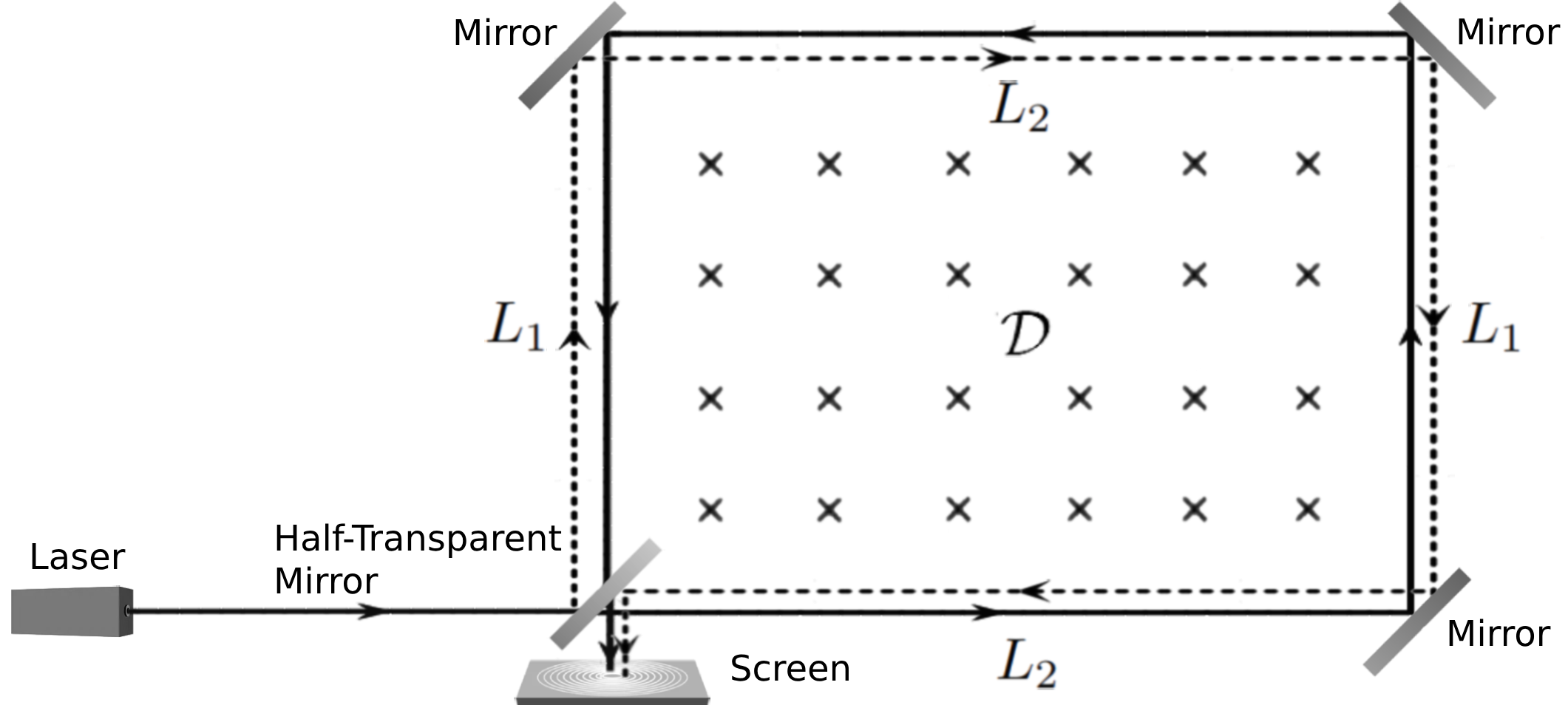
Figure 1: Measurement of spin memory effect

Proceeding as in (4.5) of PSZ , we obtain

$$\Delta\tau=\frac{1}{|\partial\mathcal{D}|}\int_{u}du\oint_{\partial\mathcal{D}}(\overset{\circ}{\operatorname{div}}\,\Theta)_{A}dx^{A}.$$ (31)

Consequently, applying Green’s theorem, it follows

$$\oint_{\partial\mathcal{D}}(\overset{\circ}{\operatorname{div}}\,\Theta)_{A}dx^{A} =\iint_{\mathcal{D}}\operatorname{curl}(\overset{\circ}{\operatorname{div}}\,\Theta)\,dx^{1}\wedge dx^{2}$$

$$=r^{-1}\iint_{\mathcal{D}}\mathcal{Q}\,dx^{1}\wedge dx^{2},$$

where we used our newly established (15). Hence, back to (31), we deduce

$$\Delta\tau=\frac{1}{r|\partial\mathcal{D}|}\int_{u}du\iint_{\mathcal{D}}\mathcal{Q}\,dx^{1}\wedge dx^{2}.$$ (32)

Recall that, from (11) we have

$$\mathcal{Q}=\int_{u}\lim_{C_{u},r\to\infty}\nabla_{3}\left(r^{3}\,\sigma\right)du-\frac{1}{2}\Theta\wedge{\underline{\Theta}}.$$

Compared with (19), we can see that part of our angular momentum memory is reflected in the spin memory effect. The formula (32) also has an explanation rooted in the classic electromagnetic theory. The quantity $\mathcal{Q}$ represents the magnetic part of the memory effect. According to Faraday’s Law, when a closed loop is placed in a changing magnetic field, an electric current will be induced in the loop, which causes the time delay.

Acknowledgements.—The authors would like to thank Sergiu Klainerman and Jérémie Szeftel for many helpful discussions and remarks. The authors would also like to thank Jiandong Zhang for a valuable discussion on spin memory.

References

• (1) A. Ashtekar, T. De Lorenzo, N. Khera and B. Krishna, Inferring the gravitational wave memory for binary coalescence events, Phys. Rev. D, 103 (2021), 044012.
• (2) L. Bieri, An extension of the stability theorem of the Minkowski space in general relativity, PhD thesis, 17178, ETH, Zürich, (2007).
• (3) L. Bieri, New effects in gravitational waves and memory, Phys. Rev. D, 103 (2021), 024043.
• (4) L. Bieri and D. Garfinkle, An electromagnetic analog of gravitational wave memory, Classical Quant. Grav. 30 (19) (2013), 195009.
• (5) P. N. Chen, M. T. Wang and S. T. Yau, Quasilocal angular momentum and center of mass in general relativity, Adv. Theor. Math. Phys. 20 (2016), 671–682.
• (6) P. N. Chen, M. T. Wang, Y.-K. Wang and S. T. Yau, Supertranslation invariance of angular momentum, Adv. Theor. Math. Phys. 25, no. 3 (2021), 777–789.
• (7) D. Christodoulou, Nonlinear Nature of Gravitation and Gravitational Wave Experiments, Phys. Rev. Lett., 67, no. 12 (1991), 1486–1489.
• (8) D. Christodoulou and S. Klainerman, The Global Nonlinear Stability of Minkowski Space, Princeton Mathematical Series 41, (1993).
• (9) E. Giorgi, S. Klainerman and J. Szeftel, Wave equations estimates and the nonlinear stability of slowly rotating Kerr black holes, arXiv:2205.14808.
• (10) R. P. Kerr, Gravitational field of a spinning mass as an example of algebraically special metrics, Phys. Rev. Letters, 11, 237, (1963).
• (11) S. Klainerman and F. Nicolò, The Evolution Problem in General Relativity. Prog. Theor. Phys., 25, Birkhauser, Boston, (2003).
• (12) S. Klainerman and F. Nicolò, Peeling properties of asymptotic solutions to the Einstein vacuum equations, Classical Quant. Grav. 20 (2003), 3215–3257.
• (13) S. Klainerman and J. Szeftel, Global nonlinear stability of Schwarzschild spacetime under polarized perturbations, Annals of Mathematics Studies 210. Princeton University Press, (2020).
• (14) S. Klainerman and J. Szeftel, Construction of GCM spheres in perturbations of Kerr, Ann. PDE 8 (2), Art. 17 (2022), 153 pp.
• (15) S. Klainerman and J. Szeftel, Effective results in uniformization and intrinsic GCM spheres in perturbations of Kerr, Ann. PDE 8 (2), Art. 18 (2022), 89 pp.
• (16) S. Klainerman and J. Szeftel, Kerr stability for small angular momentum, Pure Appl. Math. Q. 19 (3) (2023), 791–1678.
• (17) E. Newman and R. Penrose, An approach to gravitational radiation by a method of spin coefficients, J. Math. Phys. 3 (1962), 566–578.
• (18) S. Pasterski, A. Strominger and A. Zhiboedov, New gravitational memories, J. High Energy Phys., 53, (2016).
• (19) A. Rizzi, Angular momentum in General Relativity: A new definition, Phys. Rev. Lett., 81, no. 6 (1998) 1150–1153.
• (20) D. Shen, Construction of GCM hypersurfaces in perturbations of Kerr, Ann. PDE 9 (1), Art. 11 (2023), 112 pp.
• (21) D. Shen, Stability of Minkowski spacetime in exterior regions, arXiv:2211.15230, to appear in Pure Appl. Math. Q..
• (22) D. Shen, Global stability of Minkowski spacetime with minimal decay, arXiv:2310.07483.