Fluttering without wind: Stokesian quasiperiodic settling

Abstract

Fluid inertia imparts rich dynamics to leaves falling from trees. We show that bodies with two planes of symmetry can display a range of behaviours even without inertia. Any such body supports a conserved quantity in its dynamics, and is either a settler, a drifter or a flutterer, depending only on its shape. At large time, settlers and drifters respectively fall vertically and obliquely, while flutterers rotate forever while executing intricate patterns. The dynamics of flutterers decouples into a periodic and a Floquet part with different time scales, giving periodicity or quasiperiodicity. We design a set of bodies and use the boundary integral method to show that settlers, drifters and flutterers, all lie in this set.

The complex and poetic dance of falling autumn leaves is a high Reynolds number phenomenon, which depends crucially on vortex shedding, a feature absent in Stokes flow [1, 2, 3]. One would therefore expect settling at zero Reynolds number to be uneventful, especially if the body has a high degree of symmetry in its shape. In fact, in steady Stokes flow, the linear and angular motion of a body with three planes of symmetry, like a sphere or an ellipsoid, are completely decoupled, and in absence of an external torque it can only display linear motion at constant velocity [4, 5, 6]. Bodies with fewer symmetries, however, can couple their translation and rotation dynamics, opening up richer possibilities. One of the consequences of this coupling is the chiral sedimenting trajectories observed for chiral body shapes, such as helices and Kelvin’s isotropic helicoid. [7, 8, 9].

Apart from complexity in body shape, another way of coupling rotation and translation in a body is through hydrodynamic interactions with other bodies [4, 5, 10, 11]. For example, two spheroids have been shown [12] to display periodic sedimentation in direct analogy with Kepler’s orbit.

A coupling between translation and rotation is not the only way to obtain non-trivial Stokesian dynamics, even in a single body. An externally imposed background flow such as shear can achieve this. The angular velocity provided by simple shear can cause an ellipsoid, despite its high symmetry, and also a body with two planes of symmetry, to go into chaotic orbits [13, 14].

Our interest is in the sedimentation of a single achiral body in zero background flow. Ellipsoids have been well-studied, and we go a step further by letting go of only one of the symmetries. We opt for bodies with two planes of symmetry, which support a particularly simple translation-rotation coupling, unlike ellipsoids, which have none. We show that all bodies of this description fall into one of three classes: settlers, drifters and flutterers, as we term them. Settlers asymptotically adopt an orientation and fall vertically, while drifters asymptotically attain a constant velocity with both horizontal and vertical components. Flutterers are the most interesting, showing quasiperiodic or periodic, but never chaotic, motion. We show that the dynamics is completely described by an overlaying of Floquet dynamics in one of the horizontal projections of the body-fixed coordinates on the periodic dynamics of the vertical projections. Our predictions are supported by recent experiments on a U-shaped disk [15] which falls into our class of flutterers. We design a set of bodies containing settlers, drifters and flutterers, and obtain their resistance matrix, which relates the external forces to particle motion, numerically by the boundary integral method. The design involves replacing the circular cross-section of a bent capsule by a concavo-convex one (see figure 1). We shall return to this specific set of bodies later but our derivation and findings hold for any body with two planes of symmetry.

In the over-damped limit where we work, gravity acting on the body is balanced by the viscous drag. The Stokesian dynamics is conveniently written in the body-fixed coordinate system of unit vectors $\{\bm{p}_{1},\bm{p}_{2},\bm{p}_{3}\}$ shown in figure 1, as

$$\begin{pmatrix}F_{1}\\ F_{2}\\ F_{3}\\ 0\\ 0\\ 0\\ \end{pmatrix}=\underbrace{\begin{pmatrix}A_{1}&0&0&0&0&B_{31}\\ 0&A_{2}&0&0&0&0\\ 0&0&A_{3}&B_{13}&0&0\\ 0&0&B_{13}&C_{1}&0&0\\ 0&0&0&0&C_{2}&0\\ B_{31}&0&0&0&0&C_{3}\\ \end{pmatrix}}_{\cal R}\begin{pmatrix}U_{1}\\ U_{2}\\ U_{3}\\ \Omega_{1}\\ \Omega_{2}\\ \Omega_{3}\\ \end{pmatrix},$$ (1)

where $\bm{F}=F_{1}\bm{p}_{1}+F_{2}\bm{p}_{2}+F_{3}\bm{p}_{3}$ is the external force, and $\bm{U}=U_{1}\bm{p}_{1}+U_{2}\bm{p}_{2}+U_{3}\bm{p}_{3}$ and $\bm{\Omega}=\Omega_{1}\bm{p}_{1}+\Omega_{2}\bm{p}_{2}+\Omega_{3}\bm{p}_{3}$ the translational and angular velocities respectively. Note that the external torque about the center of mass is zero. Equation 1 has been is non-dimensionalized by characteristic length and time scales $L$ and $\tau$ of the body, with $\tau=\eta L^{2}/(mg_{r})$, $\eta$ being the fluid viscosity, and $mg_{r}$ the buoyancy-corrected weight of the body. All entries in the resistance matrix $\cal R$ depend only on the body shape and are invariant under overall size-scaling due to our non-dimensionalisation. We note that the two planes of symmetry allow for translation-rotation coupling of a particularly simple form, with two independent entries $B_{13}$ and $B_{31}$. The rotation matrix $\bm{R}$ connects the lab-fixed coordinate axes to the body-fixed coordinate axes as: $\bm{p}_{i}=\bm{R}_{ji}\bm{e}_{j}$, $i,j\in\{1,2,3\}$ with $\bm{e}_{1}=\bm{\hat{x}},\bm{e}_{2}=\bm{\hat{y}}$ and $\bm{e}_{3}=\bm{\hat{z}}$. So, in the lab frame

$$\bm{R}=\begin{pmatrix}p_{1x}&&p_{2x}&&p_{3x}\\ p_{1y}&&p_{2y}&&p_{3y}\\ p_{1z}&&p_{2z}&&p_{3z}\end{pmatrix},\quad\bm{R}^{T}\bm{R}=\bm{R}\bm{R}^{T}=\mathbb{I}.$$ (2)

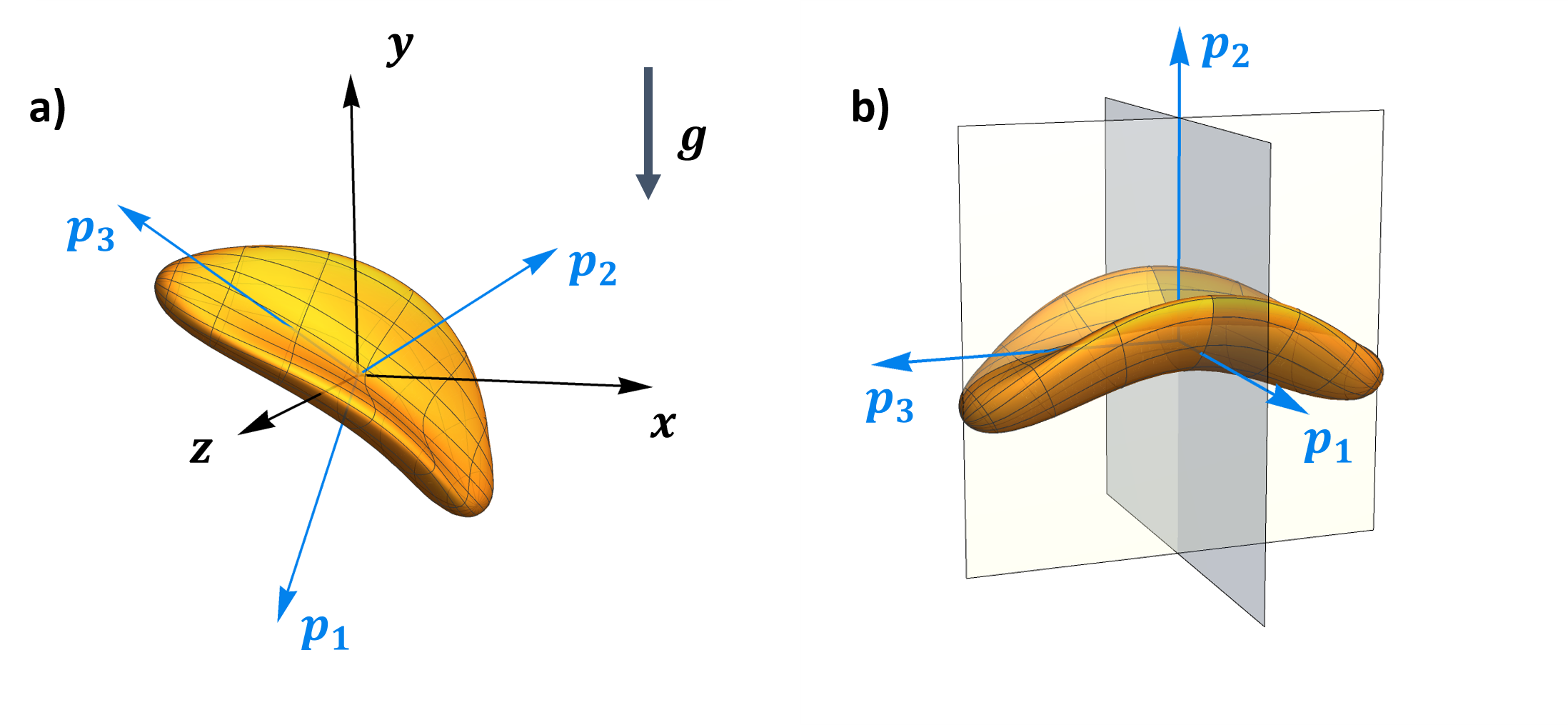
Figure 1: (a) A saddle-shaped body with two mutually perpendicular planes of symmetry, with principal axes $\bm{p}_{1}$, $\bm{p}_{2}$ and $\bm{p}_{3}$. The lab-fixed coordinate axes are $x$, $y$ and $z$ axes, $y$ being anti-parallel to gravity $\bm{g}$. (b) Note that $\bm{p}_{1}-\bm{p}_{3}$ is not a plane of symmetry.

We define two parameters $\alpha_{p}$ and $\alpha_{r}$ as:

$$\alpha_{p}=\frac{B_{13}}{A_{3}C_{1}-B_{13}^{2}},\quad\alpha_{r}=\frac{B_{31}}{A_{1}C_{3}-B_{31}^{2}},$$ (3)

which are functions only of the shape of the body. The pitching rate $\Omega_{1}$ and the rolling rate $\Omega_{3}$ are proportional to the two parameters $\alpha_{p}$ and $\alpha_{r}$, respectively. We obtain a fortunate decoupling of the dynamics of the vertical projections of the body’s coordinates from that of their horizontal projections. However, the horizontal projections depend on the vertical projections, as we shall see. For the vertical projections, using equations (1), (2) and $\bm{\dot{p}}_{i}=\bm{\Omega}\times\bm{p}_{i},\,i\in\{1,2,3\}$, we get

$$\dot{p}_{1y}=\alpha_{r}p_{1y}p_{2y},$$ (4a)

$$\dot{p}_{2y}=\alpha_{p}p_{3y}^{2}-\alpha_{r}p_{1y}^{2},$$ (4b)

$$\dot{p}_{3y}=-\alpha_{p}p_{3y}p_{2y},$$ (4c)

with the constraint $|\bm{p}_{y}|^{2}=1$, where $\bm{p}_{y}\equiv(p_{1y},p_{2y},p_{3y})$, as required by equation (2). Equation (4) admits a conserved quantity given by

$$H=|p_{1y}|^{\alpha_{p}}|p_{3y}|^{\alpha_{r}}.$$ (5)

The great circles given by $p_{1y}=0$ and $p_{3y}=0$ are invariant solutions of equation (4), which means that the sign of $p_{1y}$ and $p_{3y}$ is preserved throughout the dynamics of $\bm{p}_{y}$. We have exploited this to define $H$ in terms of absolute values of $p_{1y}$ and $p_{3y}$ to ensure that $H$ remains a positive real number. The conserved quantities $H$ and $|\bm{p}_{y}|^{2}=1$ render the system (4) integrable. The solutions lie on the intersection of the unit sphere $\mathcal{S}^{2}$ with surfaces of constant $H$.

The dynamical system described by equation (4) has fixed points given by:

$$\bm{p}_{y}^{*}=\{0,\pm 1,0\}\cup\left\{\pm\sqrt{\frac{\alpha_{p}}{\alpha_{p}+\alpha_{r}}},0,\pm\sqrt{\frac{\alpha_{r}}{\alpha_{p}+\alpha_{r}}}\right\},$$ (6)

and presents three different dynamics for bodies whose $\alpha_{p}\alpha_{r}\lesseqgtr 0$, as seen in their phase portraits in figure 2.

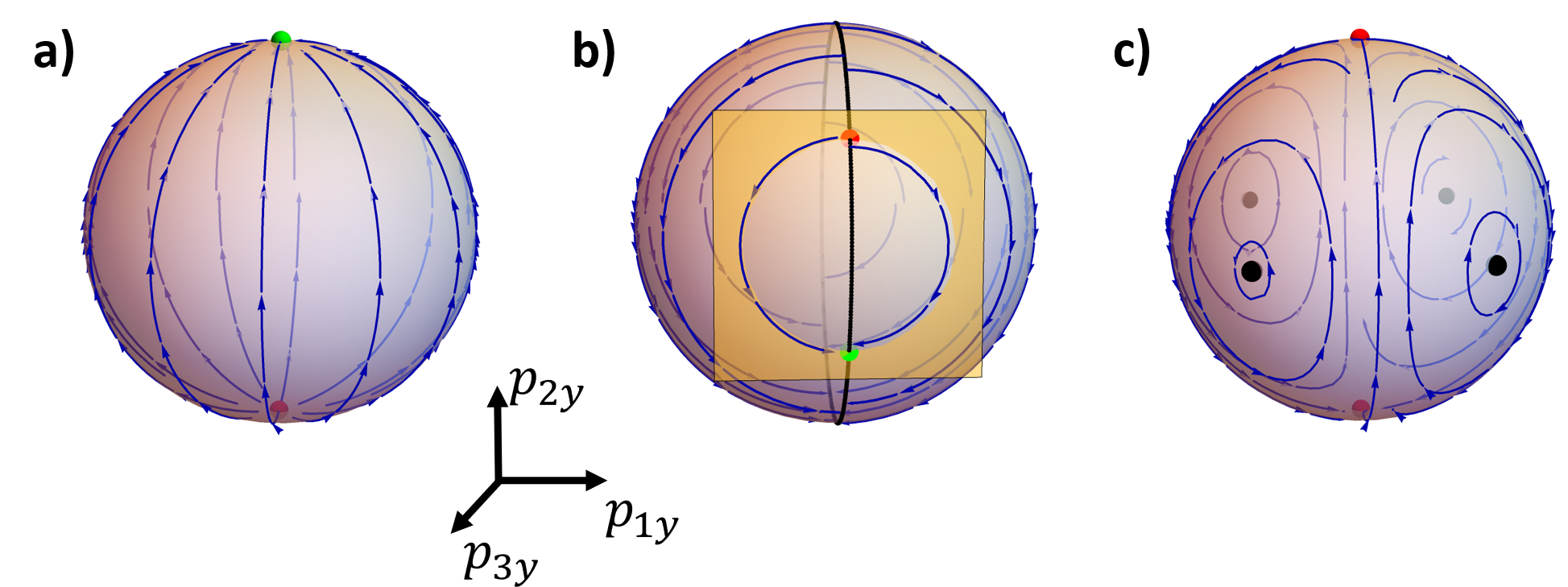
Figure 2: Phase portraits of the $\bm{p}_{y}$ dynamical system. Red, green and black dots denote unstable, stable and center fixed points, respectively, and blue lines with arrows are sample trajectories. (a) Settlers eventually fall vertically down with their $\bm{p}_{2}$ axis parallel/anti-parallel to gravity. (b) Drifters at long times sediment with horizontal drift, with their principal axes oriented obliquely with gravity. The beige plane represents a particular $H$. (c) Flutterers rotate forever as they fall, performing periodic or quasi-periodic orbits.

Bodies with $\alpha_{p}\alpha_{r}<0$ are termed ‘settlers’, whose phase portrait has one stable and one unstable fixed point. From any initial orientation, settlers attain their stable orientation, with their $\bm{p}_{2}$ parallel/anti-parallel to gravity, asymptotically in time, and thence fall vertically. The stable fixed point is globally attracting (see appendix A). A bent capsule with circular cross-section, for example, is a settler.

The class we term ‘drifters’ have $\alpha_{p}\alpha_{r}=0$. Their dynamics sustains infinitely many fixed points lying along the great circle, which we term $\cal A$, of $p_{1y}=0$ if $\alpha_{p}=0$ or $p_{3y}=0$ if $\alpha_{r}=0$. The dynamics occur in the intersection of $\mathcal{S}^{2}$ with the plane of constant $p_{3y}$ ($p_{1y}$), provided $\alpha_{p}=0$ ($\alpha_{r}=0$). This invariant manifold (a circle) contains two points of intersection with $\cal A$, one stable and the other unstable, as shown in figure 2(b). Drifters will eventually fall with their principal axes inclined at some constant angles with respect to gravity. Thus, like ellipsoids, drifters display persistent horizontal drift.

A wide range of behaviour, all involving rotation for all time, is displayed by ‘flutterers’, whose $\alpha_{p}\alpha_{r}>0$. Every fixed point here is either a center or a saddle point. The maximum in $H$,

$$H_{\text{max}}=\dfrac{|\alpha_{p}|^{|\alpha_{p}|/2}|\alpha_{r}|^{|\alpha_{r}|/2}}{(|\alpha_{p}|+|\alpha_{r}|)^{|\alpha_{p}|/2+|\alpha_{r}|/2}},$$ (7)

corresponds to center fixed points and the minimum, $H_{\text{min}}=0$, corresponds to stable and unstable manifolds of the saddle points. The trajectory for a given initial condition lies on one of the four closed curves formed by intersection of $\mathcal{S}^{2}$ with the corresponding constant $H$ surface (figure 3),

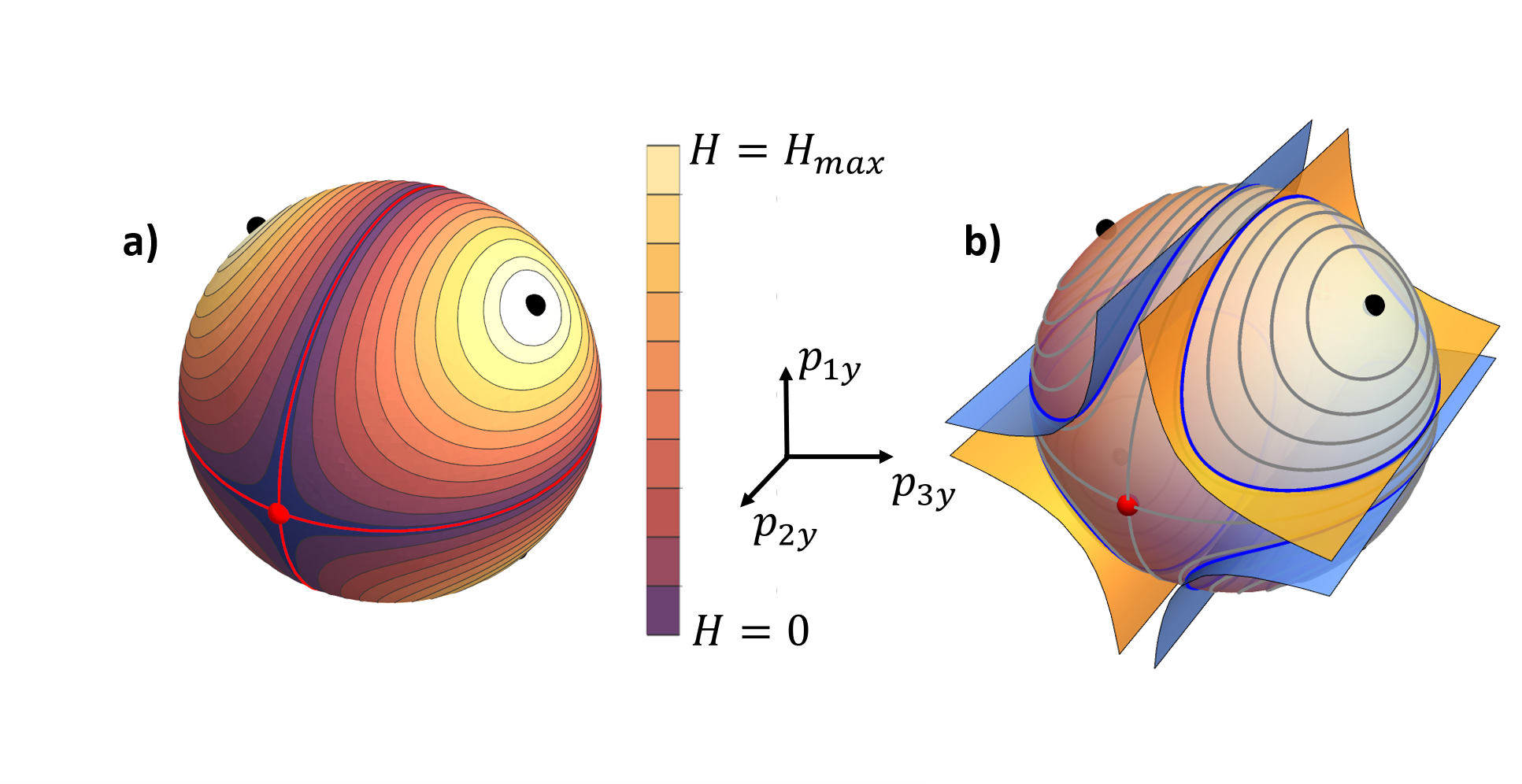
Figure 3: (a) Contour plot of the conserved quantity $H$. Its maximum, $H_{\text{max}}$, corresponds to fixed points of the $\bm{p}_{y}$ dynamics (black dots). The great circles in red, where $H=0$, are the stable and unstable manifolds of the saddle points denoted by red dots, which divide $\mathcal{S}^{2}$ into four regions. Each trajectory of constant $H$ lives on one of the four closed regions. (b) Trajectories on the yellow surfaces with $p_{1y}p_{3y}>0$ have different translational chirality from those with $p_{1y}p_{3y}<0$ which lie on the blue surfaces, as discussed later.

indicating periodic behaviour of $\bm{p}_{y}$. The time period $T_{y}$ of orbits near the center fixed points can be obtained after linearizing equation (4) about them: $\lim_{H\to H_{\text{max}}}T_{y}\equiv T_{ym}=2\pi/\sqrt{2\alpha_{p}\alpha_{r}}$. Also $T_{y}$ everywhere can be obtained numerically, and is shown in figure 4. Flutterers of different shapes show qualitatively similar trends in time period.

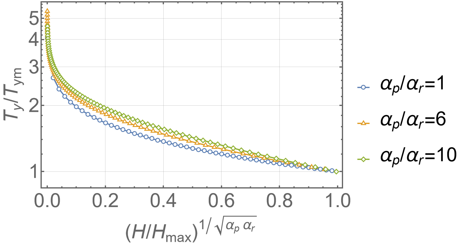
Figure 4: Dependence of the time period of the $\bm{p}_{y}$ dynamics of flutterers on the conserved quantity $H$. As $H\to H_{\text{max}}$, $T_{y}\to T_{ym}$. As $H\to 0$, trajectories spend longer durations close to the saddle points, and $T_{y}$ can increase without bound. A given ratio $\alpha_{p}/\alpha_{r}$ and its inverse yield the same curve.

The equation (4) only describes the rotational dynamics up to a rotation about the $y$-axis. To capture the remaining part of the dynamics we write equations for the projection of $\bm{p}_{i}$’s along the $x$-axis of the lab frame:

$$\begin{pmatrix}\dot{p}_{1x}\\ \dot{p}_{2x}\\ \dot{p}_{3x}\end{pmatrix}=\bm{A}(t)\begin{pmatrix}p_{1x}\\ p_{2x}\\ p_{3x}\end{pmatrix},$$ (8a)

$$\bm{A}(t)\equiv\begin{pmatrix}0&&\alpha_{r}p_{1y}(t)&&0\\ -\alpha_{r}p_{1y}(t)&&0&&\alpha_{p}p_{3y}(t)\\ 0&&-\alpha_{p}p_{3y}(t)&&0\\ \end{pmatrix}.$$ (8b)

Note that equation (2) provides three constraints:

$$|\bm{p}_{y}(t)|^{2}=1,$$ (9a)

$$|\bm{p}_{x}(t)|^{2}=1,$$ (9b)

$$\bm{p}_{x}(t)\cdot\bm{p}_{y}(t)=0,\quad\forall\quad t.$$ (9c)

Equations (4), (8) and (9) fully describe the rotational dynamics of the body. Equation (8) shows that $\bm{p}_{x}$ is driven by $\bm{p}_{y}$. Since the latter is time-periodic, $\bm{p}_{x}(t)$ can be solved using Floquet theory [16]. We define a $T_{y}$ period Poincare map of the $\bm{p}_{x}$ dynamical system as:

$$\mathcal{P}_{t_{0}}^{t_{0}+T_{y}}=\bm{\Phi}_{t_{0}}^{t_{0}+T_{y}},\quad$$ (10a)

$$\bm{\dot{\Phi}}_{t_{0}}^{t}=\bm{A}(t)\bm{\Phi}_{t_{0}}^{t};\quad\bm{\Phi}_{t_{0}}^{t_{0}}=\mathbb{I},$$ (10b)

where $\bm{\Phi}_{t_{0}}^{t}$ is the solution operator of equation (8), i.e., $\bm{p}_{x}(t)=\bm{\Phi}_{t_{0}}^{t}\bm{p}_{x}(t_{0})$. Since $\bm{A}^{T}(t)=-\bm{A}(t)$, equation (10) ensures that $\bm{\Phi}_{t_{0}}^{t}\in SO(3)$. Therefore, both the solution operator and the Poincare map correspond to some 3D rotations. Consequently, the eigenvalues of the Poincare map are given by $1$ and $e^{\pm i\mu T_{y}}$, where $\mu\in\mathbb{R}$ is the Floquet exponent. The constraints of (9) restrict $\bm{p}_{x}(t)$ to lie normal to $\bm{p}_{y}(t)$. Since $\bm{p}_{y}(t_{0}+T_{y})=\bm{p}_{y}(t_{0})$, the image set of the Poincare map $\{\mathcal{P}_{t_{0}}^{t_{0}+nT_{y}}\bm{p}_{x}(t_{0})\}_{n\in\mathbb{N}}$ is a subset of the great circle lying normal to $\bm{p}_{y}(t_{0})$. Thus, the Poincare map $\mathcal{P}_{t_{0}}^{t_{0}+T_{y}}$ acting on $\bm{p}_{x}$ corresponds to the rotation of $\bm{p}_{x}$ by an angle $\theta\equiv\mu T_{y}$ about the axis $\bm{p}_{y}(t_{0})$. It is shown in the supplementary material that the eigenvalues of the Poincare map are independent of the initial time $t_{0}$. So the rotation angle $\theta=\mu T_{y}$ is only a function of $H$. By Floquet theory, any solution of equation (8) can be decomposed as

$$\bm{p}_{x}(t)=e^{i\mu t}\bm{b}(t),$$ (11)

where $\bm{b}(t)=\bm{b}(t+T_{y})$ is some $T_{y}$-periodic function. Thus, if the driving frequency $\omega_{y}\equiv 2\pi/T_{y}$ is incommensurate with the response frequency $\mu$, i.e., if $\theta/2\pi=\mu/\omega_{y}$ is an irrational number, flutterers’ motion is quasi-periodic, whereas if it is rational we have periodic dynamics. In the quasi-periodic case the image set of the Poincare map fills up the entire great circle.

Figure 5 shows the dependence of the frequency ratio on $H$.

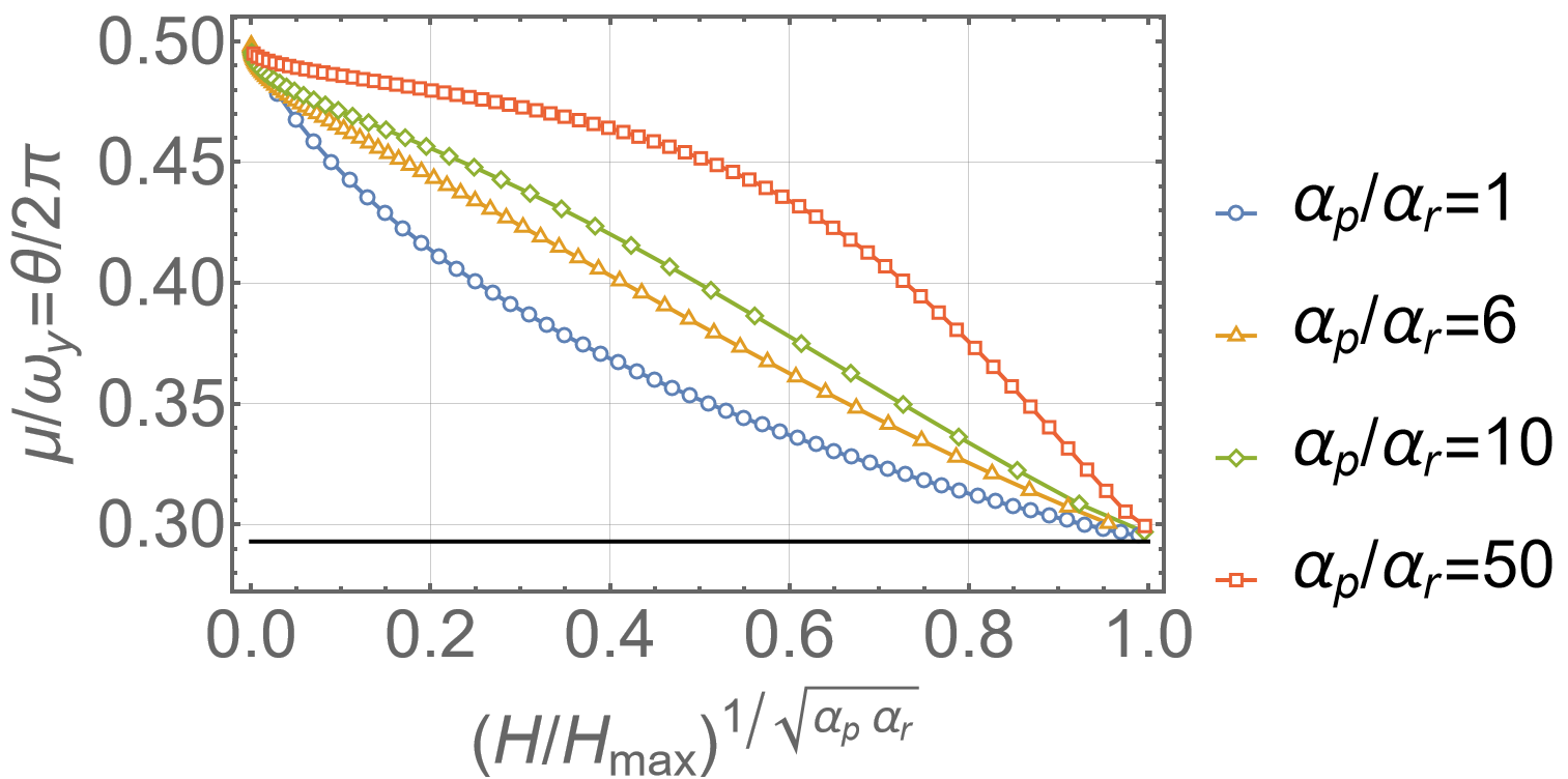
Figure 5: The $\bm{p}_{x}$ dynamics of flutterers involves two frequencies, $\mu$ and $\omega_{y}$. Their ratio, which is equivalent to the rotation angle $\theta/2\pi$ of the Poincare map, is shown here.

There are differences in detail for different ratios of $\alpha_{r}$ and $\alpha_{p}$, but in all cases, the frequency ratio varies continuously on the interval $[1-1/\sqrt{2},\,0.5]$ which is therefore dense in periodic and quasi-periodic orbits. Figure 6 shows phase trajectories and image sets of Poincare maps for a periodic and quasi-periodic case.

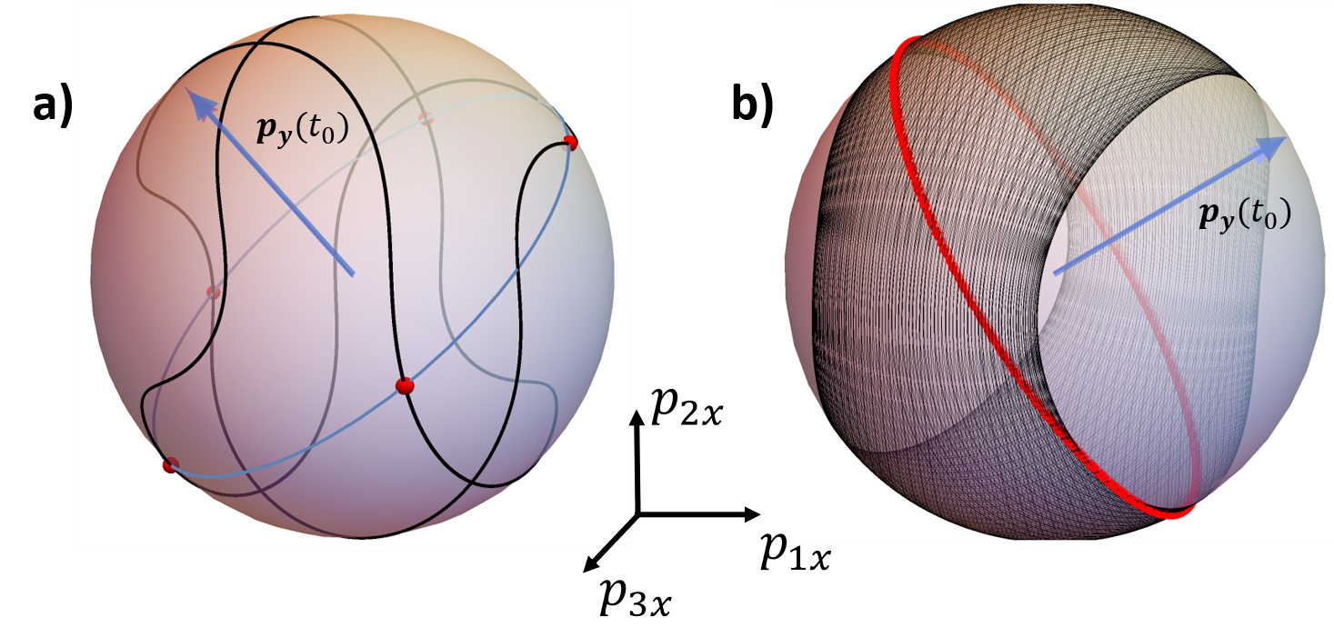
Figure 6: Sample $\bm{p}_{x}$ trajectories shown as black curves on $\mathcal{S}^{2}$. (a) Period-5 trajectory. The red dots show the Poincare map $\mathcal{P}_{t_{0}}^{t_{0}+T_{y}}$ which lie on the great circle shown by the blue curve. This great circle lies normal to $\bm{p}_{y}(t_{0})$. (b) Quasi-periodic trajectory. The Poincare map covers the entire great circle lying normal to $\bm{p}_{y}(t_{0})$. The filled region has the inversion symmetry $\bm{p}_{x}\to-\bm{p}_{x}$.

Another class of periodic orbits are obtained on the center fixed points of the $\bm{p}_{y}$ dynamics, characterized by $H=H_{\text{max}}$. In this case $\bm{A}(t)=\bm{A}^{*}$ is a constant matrix with the eigenvalues $0,\pm i\sqrt{\alpha_{p}\alpha_{r}}$. The eigenvector corresponding to the zero eigenvalue is not orthogonal to $\bm{p}_{y}$, and is dropped from the discussion since it violates the constraints.

The translational velocity of any of these three classes of bodies can be obtained from equations (1) and (2). In the lab frame

$$v_{x}=-G_{1}p_{1x}p_{1y}-G_{2}p_{2x}p_{2y}-G_{3}p_{3x}p_{3y},$$ (12a)

$$v_{y}=-G_{1}p_{1y}^{2}-G_{2}p_{2y}^{2}-G_{3}p_{3y}^{2},$$ (12b)

$$v_{z}=-G_{1}p_{1z}p_{1y}-G_{2}p_{2z}p_{2y}-G_{3}p_{3z}p_{3y},$$ (12c)

where $(p_{1z},p_{2z},p_{3z})\equiv\bm{p}_{z}\equiv\bm{p}_{x}\times\bm{p}_{y}$, $G_{2}\equiv 1/A_{2}$ and

$$G_{1}\equiv\frac{C_{3}}{A_{1}C_{3}-B_{31}^{2}},\quad G_{3}\equiv\frac{C_{1}}{A_{3}C_{1}-B_{13}^{2}}.$$ (13)

Viscous dissipation requires $G_{1},G_{2},G_{3}>0$ [4, 5]. Equation (12) shows direct dependence of translational velocity on the orientation of the body. Thus, periodicity in ${\mathbf{p}}_{y}$ implies periodicity in $v_{y}$, and quasi-periodicity in ${\mathbf{p}}_{x}$ implies quasi-periodicity in the horizontal components of the velocity. It is relevant to ask if there a persistent drift in the horizontal plane. This must be answered separately for the quasi-periodic and the periodic cases. For the former, following Thorp and Lister [14] we exploit the discrete symmetries of the rotational dynamical equations to rule out persistent drift. Note that $v_{x}(\bm{p}_{y},\bm{p}_{x})=-v_{x}(\bm{p}_{y},-\bm{p}_{x})$, $v_{z}(\bm{p}_{y},\bm{p}_{x})=-v_{z}(\bm{p}_{y},-\bm{p}_{x})$, a quasi-periodic trajectory which explores $(\bm{p}_{y},\bm{p}_{x})$ must explore $(\bm{p}_{y},-\bm{p}_{x})$ (see appendix C). Thus, any drift at one point in time is exactly cancelled by the opposite drift at some other point in time. For the periodic case with $H\neq H_{\text{max}}$, persistent drift can occur in the horizontal plane only if the response frequency $\mu$ is exactly equal to the driving frequency $\omega_{y}$ (see appendix C). In other words, the Poincare map $\mathcal{P}_{t_{0}}^{t_{0}+T_{y}}$ now is the identity matrix. When $H=H_{\text{max}}$, we will still have no persistent drift, since the valid solutions of $\mathbf{p}_{x}$ are periodic with zero mean. Finally, for $H=0$, the body exponentially reaches the saddle point $\bm{p}_{y}^{*}=(0,\pm 1,0)$ along its stable manifold as $t\to\infty$ and consequently the horizontal drift goes to zero exponentially.

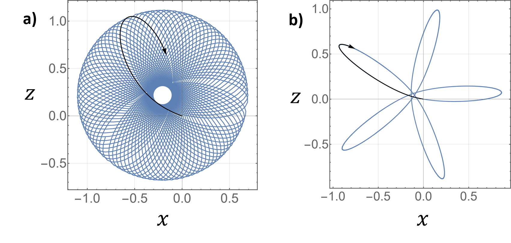
Figure 7: Translational trajectories in the horizontal plane for sample (a) quasi-periodic and (b) periodic orbits. With gravity pointing out of the plane, the trajectories move clockwise in this view, which we classify as negative chirality.

We now discuss the chirality of the translational trajectories. As the body settles, its motion in the horizontal $x-z$ plane is either clockwise or anti-clockwise when viewed from below, corresponding to negative or positive chirality respectively. As mentioned in figure 3, regions on $\mathcal{S}^{2}$ with $p_{1y}p_{3y}>0$ correspond to different chirality in translation motion from regions with $p_{1y}p_{3y}<0$. This can be seen as follows: for any given angular trajectory ($\bm{p}_{y},\bm{p}_{x}$) with $p_{1y}p_{3y}>0$, the transformation $g:(p_{1y},\,p_{1x})\to(-p_{1y},\,-p_{1x})$ maps the original trajectory to the trajectory in the region $p_{1y}p_{3y}<0$ with the same $H$. Thus the mapped trajectory has same time period $T_{y}$ in $\bm{p}_{y}$ dynamics and same frequency ratio $\mu/\omega_{y}$ in $\bm{p}_{x}$ dynamics. However, $g:v_{z}\to-v_{z}$, while the other velocity components remain invariant. So the trajectory of the translational dynamics ($x(t),y(t),z(t)$) is mapped to the trajectory $(x(t),y(t),-z(t))$, i.e., the original and mapped trajectories are of opposite chirality.

The vertical sedimentation velocity $v_{y}$ is $T_{y}$-periodic because it only depends on $\bm{p}_{y}$. Thus, for a given body the mean sedimentation velocity $\langle v_{y}\rangle$ averaged over $T_{y}$ only depends on $H$. For $H=0$, $v_{y}$ reaches $v_{y0}=-G_{2}$ exponentially fast in time with the rate $|\alpha_{p}|$ or $|\alpha_{r}|$, depending on the initial condition, and for $H=H_{\text{max}}$, $v_{y}=v_{ym}\equiv-(G_{1}\alpha_{p}+G_{3}\alpha_{r})/(\alpha_{p}+\alpha_{r})$. The shape of the body determines whether $\langle v_{y}\rangle$ increases or decreases with $H$, and a sample of each is shown in figure 8.

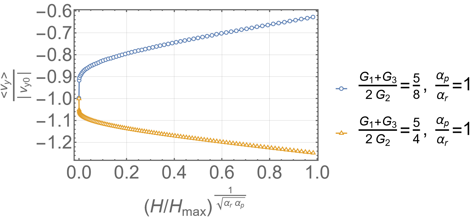
Figure 8: Dependence of mean vertical sedimentation velocity on $H$. Depending on the shape of the body, the periodic/quasi-periodic dynamics $H\neq 0$ can result in either slower or faster settling velocity as compare to the case where it falls along a stable manifold of saddle points $H=0$.

It remains to obtain the resistance matrix $\cal R$, and thence $\alpha_{p}$ and $\alpha_{r}$, for a given body shape. To define the set of bodies we have used two shape-controlling non-dimensional parameters: the bending parameter $a$, and the concavity parameter $b$, as shown in figure 9. Further details are available in supplementary E.

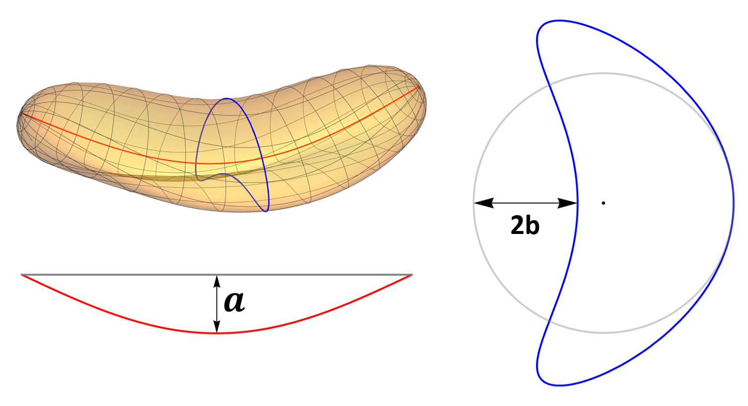
Figure 9: Our set of bodies is defined by the two parameters $a$ and $b$ shown here. The body shown is a flutterer.

We develop and use a numerical solver to find the resistance matrix $\cal R$ by the Boundary Integral Method [5, 17, 18, 19, 20]. The five parameters $\alpha_{p},\,\alpha_{r},\,G_{1},\,G_{2},\,G_{3}$ completely describe the sedimentation problem in a quiescent fluid.

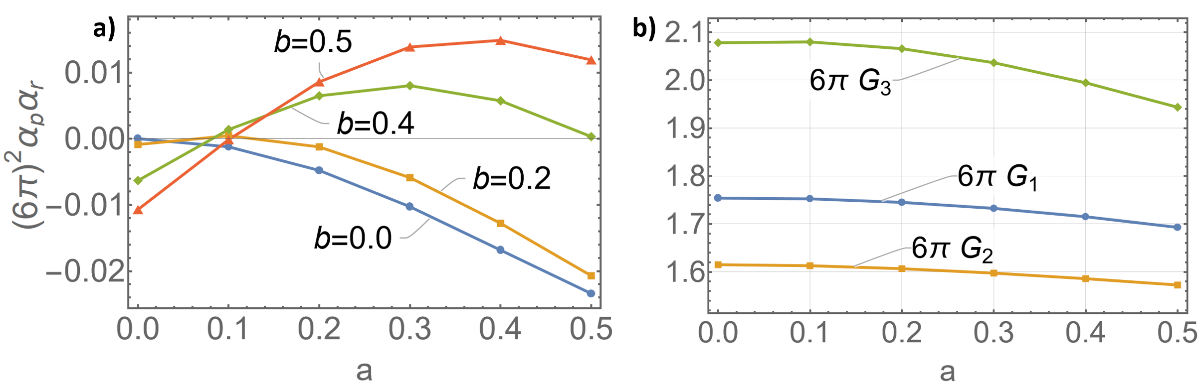
Figure 10: As $a$ and $b$ in figure 9 are varied, we obtain settlers ($\alpha_{p}\alpha_{r}<0$), drifters ($\alpha_{p}\alpha_{r}=0$), and flutterers ($\alpha_{p}\alpha_{r}>0$). (a) Increasing $b$ turns settlers into flutterers, but increasing $a$ at fixed $b$ eventually turns flutterers back into settlers. (b) Dependence of parameters determining the settling velocity on the bending parameter $a$, for a fixed $b=0.4$.

To summarise, we have shown that bodies with exactly two planes of symmetry show three kinds of Stokesian sedimentation, depending only on their shape, appearing through the parameter $\alpha_{p}\alpha_{r}$. (1) Settlers with $\alpha_{p}\alpha_{r}<0$ asymptotically fall vertically without rotating, (2) Drifters with $\alpha_{p}\alpha_{r}=0$ eventually fall obliquely with respect to gravity without rotating and (3) Flutterers with $\alpha_{p}\alpha_{r}>0$ perform periodic or quasi-periodic rotational and translational motion as they sediment. The vertical projections $\bm{p}_{y}$ of their body-fixed coordinate axes executes periodic dynamics. A conserved quantity $H$ exists, the value of which decides the time period of the $\bm{p}_{y}$ dynamics. The periodic motion in $\bm{p}_{y}$ drives the dynamics of horizontal projections of body attached coordinate axes $\bm{p}_{x}$, which leads to a periodic or quasi-periodic response based on the ratio of response to driving frequency, $\mu/\omega_{y}$. This ratio too depends only on $H$. Our numerical solutions suggest that this ratio is bounded within the interval $[1-1/\sqrt{2},0.5]$, indicating that no value of $H$ corresponds to the response frequency being same as the driving frequency. For these periodic or quasi-periodic orbits there is no persistent drift in the horizontal plane. The chirality of the translational trajectories can be classified using $p_{1y}p_{3y}\lessgtr 0$. The mean sedimentation velocity of the flutterers has the same time period as the $\bm{p}_{y}$ dynamics. All three classes of bodies can be obtained by bending a capsule about its central axis and making its cross-section concavo-convex. This work highlights how rich the dynamics of sedimenting bodies can be in the presence of even simple translation-rotation coupling. Our choice of dynamical variables brings out an inherent decoupling in the rotational dynamics, providing better understanding of flutterers, and can be used to study them in background flow.

We thank Saumav Kapoor for help in designing the flutterer shape. We acknowledge support of the Department of Atomic Energy, Government of India, under project no. RTI4001.

Appendix A Lyapunov function for global stability

For settlers, which have $\alpha_{r}\alpha_{p}<0$, a Lyapunov function exists which shows that the stable fixed point is globally stable.

Consider first the case where $\alpha_{p}>0$ and $\alpha_{r}<0$: here $\bm{p}_{y}^{*1}=(0,1,0)$ is a non-hyperbolic fixed point corresponding to the eigenvalues $(0,-\alpha_{p},-|\alpha_{r}|)$. The Lyapunov function is

$$f_{1}(\bm{p}_{y})=p_{1y}^{2}+p_{3y}^{2}+(p_{2y}-1)^{2}.$$ (14)

Clearly, $f_{1}(\bm{p}_{y}^{*1})=0$ and $f_{1}(\bm{p}_{y})>0$ for $\bm{p}_{y}\neq\bm{p}_{y}^{*1}$. Now, $\dot{f}_{1}=-2(\alpha_{p}p_{3y}^{2}+|\alpha_{r}|p_{1y}^{2})<0$ for all $\bm{p}_{y}\neq\bm{p}_{y}^{*1}$, showing $\bm{p}_{y}^{*1}$ to be a globally attracting fixed point.

Similar arguments may be made for the other case, where $\alpha_{p}<0$ and $\alpha_{r}>0$, using the Lyapunov function

$$f_{2}(\bm{p}_{y})=p_{1y}^{2}+p_{3y}^{2}+(p_{2y}+1)^{2},$$ (15)

with $\bm{p}_{y}^{*1}=(0,-1,0)$ being the stable fixed point.

Appendix B Discrete and continuous symmetries of the rotational dynamics of flutterers

The discrete symmetry group of the rotational dynamical equations (4) and (8) is $\mathcal{G}_{R}=\mathbb{Z}_{2}\times\mathbb{Z}_{2}\times\mathbb{Z}_{2}$. The group $\mathcal{G}_{R}$ is an abelian group containing 8 elements which corresponds to the following eight transformations of dynamical variables:

Element	Action on ($p_{1y},\,p_{2y},\,p_{3y},\,p_{1x},\,p_{2x},\,p_{3x}$)
$e$	($p_{1y},\,p_{2y},\,p_{3y},\,p_{1x},\,p_{2x},\,p_{3x}$)
$a$ = $g\ast h$	($-p_{1y},\,p_{2y},\,-p_{3y},\,p_{1x},\,-p_{2x},\,p_{3x}$)
$b$ = $a\ast c$	($-p_{1y},\,p_{2y},\,p_{3y},\,p_{1x},\,-p_{2x},\,-p_{3x}$)
$c$ = $a\ast b$	($p_{1y},\,p_{2y},\,-p_{3y},\,p_{1x},\,p_{2x},\,-p_{3x}$)
$d$ = $a\ast f$	($p_{1y},\,p_{2y},\,-p_{3y},\,p_{1x},\,-p_{2x},\,-p_{3x}$)
$f$ = $b\ast h$	($-p_{1y},\,p_{2y},\,p_{3y},\,-p_{1x},\,p_{2x},\,p_{3x}$)
$g$ = $a\ast h$	($-p_{1y},\,p_{2y},\,-p_{3y},\,-p_{1x},\,p_{2x},\,-p_{3x}$)
$h$ = $c\ast d$	($p_{1y},\,p_{2y},\,p_{3y},\,-p_{1x},\,-p_{2x},\,-p_{3x}$)

Table 1: Discrete symmetries of rotational dynamics

The binary operations between the elements is shown in the first column of table 1. The corresponding multiplication table of this group is isomorphic to the group $\mathbb{Z}_{2}\times\mathbb{Z}_{2}\times\mathbb{Z}_{2}$. The group element $h$ is used to establish that there is no persistent drift for quasi-periodic orbits, while the element $g$ is used to show the dependence of the chirality on the sign of $p_{1y}p_{3y}$. Here we have restricted ourselves to transformations that only act on the dynamical variables and not on time $t$.

The continuous Lie symmetries of the rotational dynamics are simply scaling symmetries and time translational symmetries. The linearly independent generators of these continuous symmetries are given by

$$X_{1}=\bm{p}_{y}\cdot\bm{\nabla}_{\bm{p}_{y}}-t\partial_{t},$$ (16a)

$$X_{2}=\bm{p}_{x}\cdot\bm{\nabla}_{\bm{p}_{x}},$$ (16b)

$$X_{3}=\bm{\dot{p}}_{y}\cdot\bm{\nabla}_{\bm{p}_{y}}+\bm{\dot{p}}_{x}\cdot\bm{\nabla}_{\bm{p}_{x}},$$ (16c)

$$X_{4}=\partial_{t}.$$ (16d)

The corresponding Lie algebra of these generators is:

$$[X_{1},\,X_{2}]=0,$$ (17a)

$$[X_{1},\,X_{3}]=X_{3},\quad[X_{1},\,X_{4}]=X_{4},$$ (17b)

$$[X_{2},\,X_{3}]=[X_{2},\,X_{4}]=[X_{3},\,X_{4}]=0.$$ (17c)

The generators $X_{1}$ and $X_{2}$ correspond to scaling symmetries: $e^{\lambda X_{1}}(\bm{p}_{y},\bm{p}_{x},t)=(e^{\lambda}\bm{p}_{y},\bm{p}_{x},e^{-\lambda}t)$ and $e^{\lambda X_{2}}(\bm{p}_{y},\bm{p}_{x},t)=(\bm{p}_{y},e^{\lambda}\bm{p}_{x},t)$ while the other two generators correspond to time translation. These Lie symmetries can be used to construct the conserved quantities or the first integrals of the rotational dynamics, as described in [21]. The four generators with three unique transformations give three unique characterstics as:

$$\bm{Q}_{1}=(\bm{p}_{y}+t\bm{\dot{p}}_{y},\,t\bm{\dot{p}}_{x}),$$ (18a)

$$\bm{Q}_{2}=(0,\,0,\,0,\,\bm{p}_{x}),$$ (18b)

$$\bm{Q}_{3}=(\bm{\dot{p}}_{y},\,\bm{p}_{x}).$$ (18c)

The three co-characterstics are given by:

$$\bm{\Lambda}_{1}=(\bm{p}_{y},\,0,\,0,\,0),$$ (19a)

$$\bm{\Lambda}_{2}=(\alpha_{p}/p_{1y},\,0,\,\alpha_{r}/p_{3y},\,0,\,0,\,0),$$ (19b)

$$\bm{\Lambda}_{3}=(0,\,0,\,0,\,\bm{p}_{x}).$$ (19c)

The conserved quantity $H$ is obtained as a first integral using: $\bm{Q}_{1}\cdot\bm{\Lambda}_{2}=\alpha_{p}+\alpha_{r}+t\dfrac{d}{dt}\log(p_{1y}^{\alpha_{p}}p_{3y}^{\alpha_{r}})$. The other scalar products of $\bm{Q}$’s and $\bm{\Lambda}$’s yield the constraints (9) as the conserved quantities.

Appendix C Necessary condition for persistent horizontal drift

Claim: Flutterers can have persistent drift in the plane perpendicular to the gravity only if the driving frequency $\omega_{y}$ of the $\bm{p}_{y}$ dynamics is exactly equal to the response frequency $\mu$ of the $\bm{p}_{x}$ dynamics, i.e. $\mu=\omega_{y}$. In this case, the Poincare map $\mathcal{P}_{t_{0}}^{t_{0}+T_{y}}$ is just the identity map.
Proof: The rotational dynamical equations (4) and (8) have a discrete symmetry group $\mathcal{G}_{R}=\mathbb{Z}_{2}\times\mathbb{Z}_{2}\times\mathbb{Z}_{2}$. If a given rotational trajectory is invariant under $g\in\mathcal{G}_{R}$ and $g(v_{i})=-v_{i}$ then there can be no persistent drift along the $x_{i}$ direction for that trajectory, for the drift at one point is exactly cancelled by the other mapped point. Note that $g:(p_{1y},p_{2y},p_{3y},p_{1x},p_{2x},p_{3x})\to(p_{1y},p_{2y},p_{3y},-p_{1x},-p_{2x},-p_{3x})$ is a symmetry of equations (4) and (8) with $g(v_{x})=-v_{x}$ and $g(v_{z})=-v_{z}$. The invariance of trajectories of the rotational dynamical system under $g$ requires the inversion symmetry $\bm{p}_{x}\to-\bm{p}_{x}$.

For quasi-periodic cases, any point $\bm{p}_{x}(t)$ in a given trajectory will be mapped to the point $-\bm{p}_{x}$ at time $t+kT_{y},\,k\in\mathbb{N}$. This is due to the fact that the Poincare map $\mathcal{P}_{t}^{t+T_{y}}$ fills up the entire great circle with normal vector $\bm{p}_{y}(t)$. Since this great circle has an inversion symmetry, there exist a $k\in\mathbb{N}$ such that $\bm{p}_{x}(t+kT_{y})=-\bm{p}_{x}$. Therefore, the region occupied by quasi-periodic orbits on $S^{2}$ has inversion symmetry $\bm{p}_{x}\to-\bm{p}_{x}$. This rules out any persistent drift in the horizontal plane owing to the discrete symmetry element $g\in\mathcal{G}_{R}$.

For the periodic case we have closed trajectories subject to constraints (9) which may not have the inversion symmetry $\bm{p}_{x}\to-\bm{p}_{x}$ (see figure 6). The discrete symmetry argument to rule out persistent drift is inconclusive in this case. A necessary condition for persistent drift can be obtained as follows: Owing to the equation (11), each term in the right hand side of $v_{x}$ and $v_{z}$ in equation (12) is of the form $e^{i\mu t}f(t)$, where $f(t)=f(t+T_{y})$ is some $T_{y}$ periodic function. The contribution of such terms to the displacement over one time period $T$ of a periodic trajectory is

$$\Delta(T)\equiv\frac{1}{T}\int_{0}^{T}e^{i\mu t}f(t)\,dt=\frac{1}{T}\sum_{k\in\mathbb{Z}}\hat{f}_{k}\int_{0}^{T}e^{i(\mu+\omega_{y}k)t}\,dt,$$ (20)

where we used the Fourier expansion: $f(t)=\sum_{k\in\mathbb{Z}}\hat{f}_{k}e^{i\omega_{y}t}$ with $\omega_{y}T_{y}=2\pi$. Now, for the periodic case, $\mu/\omega_{y}=n_{1}/n_{2}\in\mathbb{Q}$, where $n_{1},n_{2}\in\mathbb{N}$ and $T=2\pi n_{2}/\omega_{y}=2\pi n_{1}/\mu$. Using these in equation (20), we have

$$\Delta(T)=\sum_{k\in\mathbb{Z}}\hat{f}_{k}\int_{0}^{1}e^{2\pi i(n_{1}+kn_{2})q}\,dq=\sum_{k\in\mathbb{Z}}\hat{f}_{k}\delta_{n_{1}+kn_{2},0},$$ (21)

where $q=t/T$. Since $k\in\mathbb{Z}$, the contribution can be non-zero if $n_{2}=1$ which implies $\mu/\omega_{y}\in\mathbb{N}$. Now, $\mu=k\omega_{y}$ for $k\in\mathbb{N}$ implies $\bm{p}_{x}(t+T_{x})=\bm{p}_{x}(t)$ with $T_{x}=T_{y}/k$. But $\bm{\dot{p}_{x}}(t+T_{x})=\bm{\dot{p}_{x}}(\bm{p}_{y}(t+T_{x}),\bm{p}_{x}(t))\neq\bm{\dot{p}}_{x}(\bm{p}_{y}(t),\bm{p}_{x}(t))$, unless $T_{y}=T_{x}$. Thus, the $\bm{p}_{x}$ trajectory cannot repeat itself after $T_{x}$ since the tangent vector $\bm{\dot{p}}_{x}$ at time $t+T_{x}$ is different from what it was at time $t$, unless $k=1$. Therefore, the only periodic trajectory for which $\Delta(T)$ can be non-zero is the case $\omega_{y}=\mu$.

Numerics suggests that the ratio $\mu/\omega_{y}$ is bounded between the interval $[1-1/\sqrt{2},\,0.5]$ in which case there is no persistent drift.

Appendix D Similarity between Poincare maps with different reference times

Consider two Poincare maps $\mathcal{P}_{t_{1}}^{t_{1}+T_{y}}$ and $\mathcal{P}_{t_{2}}^{t_{2}+T_{y}}$ with $t_{2}>t_{1}$ and $T_{y}$ the same in both the maps. These map satisfies the following equation:

$$\mathcal{P}_{t_{1}}^{t_{1}+T_{y}}=\bm{\Phi}_{t_{1}}^{t_{1}+T_{y}};\,\bm{\dot{\Phi}}_{t_{1}}^{t_{1}+t}=\bm{A}(t)\bm{\Phi}_{t_{1}}^{t_{1}+t},\,\bm{\Phi}_{t_{1}}^{t_{1}}=\mathbb{I},$$ (22a)

$$\mathcal{P}_{t_{2}}^{t_{2}+T_{y}}=\bm{\Phi}_{t_{2}}^{t_{1}+T_{y}};\,\bm{\dot{\Phi}}_{t_{2}}^{t_{2}+t}=\bm{A}(t)\bm{\Phi}_{t_{2}}^{t_{2}+t},\,\bm{\Phi}_{t_{2}}^{t_{2}}=\mathbb{I}.$$ (22b)

Claim: The two Poincare maps $\mathcal{P}_{t_{1}}^{t_{1}+T_{y}}$ and $\mathcal{P}_{t_{2}}^{t_{2}+T_{y}}$ are related by a similarity transformation
Proof: Since $\bm{\Phi}_{t_{2}}^{t_{2}+t}\bm{\Phi}_{t_{1}}^{t_{2}}=\bm{\Phi}_{t_{1}}^{t_{2}+t}$, we have,

$$\mathcal{P}_{t_{2}}^{t_{2}+T_{y}}\bm{\Phi}_{t_{1}}^{t_{2}}=\bm{\Phi}_{t_{1}}^{t_{2}+T_{y}}.$$ (23)

Now, $\bm{\Phi}_{t_{1}}^{t_{2}+T_{y}}=\bm{\Phi}_{t_{1}+T_{y}}^{t_{2}+T_{y}}\bm{\Phi}_{t_{1}}^{t_{1}+T_{y}}$. Since $\bm{A}(t+T_{y})=\bm{A}(t)$, we have:

$$\bm{\Phi}_{t_{1}}^{t_{2}}=\bm{\Phi}_{t_{1}+T_{y}}^{t_{2}+T_{y}}\implies\bm{\Phi}_{t_{1}}^{t_{2}+T_{y}}=\bm{\Phi}_{t_{1}}^{t_{2}}\bm{\Phi}_{t_{1}}^{t_{1}+T_{y}}.$$ (24)

Using this in equation (23) we get,

$$\mathcal{P}_{t_{2}}^{t_{2}+T_{y}}\bm{\Phi}_{t_{1}}^{t_{2}}=\bm{\Phi}_{t_{1}}^{t_{2}}\mathcal{P}_{t_{1}}^{t_{1}+T_{y}}.$$ (25)

Thus, the two Poincare maps are related by a similarity transformation. The eigenvalues of these maps are therefore the same, and given by $1,\,e^{\pm i\theta}$, where $\theta$ is only a function of $T_{y}$ and hence $\theta=\theta(H)$.

Appendix E Parametric equation of a set of bodies with only two planes of symmetry

A class of bodies ranging from settlers through drifters to flutterers can be constructed using a parameterization as described here. The centerline of the bodies is a bent filament which is parameterized by a parameter $s$ as:

$$\bm{r}_{c}(s)=a\cos(ks)\bm{p}_{2}+s\bm{p}_{3},\,s\in[-1,1],$$ (26)

where the parameterization is in non-dimensional form with half the size of the bent filament as the length scale, $k=\pi/2$ and $a$ is the dimensionless bending parameter (see red filament in figure 9). To construct a 2D surface, cross sections are drawn around this filament ranging from circular near the edges ($s=\pm 1$) to concavo-convex near the center $s=0$. The normal vector $\bm{n}_{c}$ and binormal vector $\bm{b}_{c}$ to the bent filament are given by

$$\bm{n}_{c}(s)=\frac{-\bm{p}_{2}-ka\sin(ks)\bm{p}_{3}}{\sqrt{1+k^{2}a^{2}\sin(ks)^{2}}}$$ (27a)

$$\bm{b}_{c}(s)=\bm{p}_{1}.$$ (27b)

The cross section of the body uses another parameter $\phi$ and can be constructed in the plane spanned by $\bm{n}_{c}$ and $\bm{b}_{c}$. The parametric equation of the class of bodies is given by

$$\bm{r}(s,\,\phi)=\bm{r}_{c}(s)+R(s)\{[(1-\hat{b}(s))\cos(\phi)$$

$$+\hat{b}(s)\cos(2\phi)]\bm{n}_{c}(s)+[(1+\hat{b}(s))\sin(\phi)$$

$$+\hat{b}(s)^{3}\sin(2\phi)]\bm{b}_{c}(s)\},$$ (28)

where $R(s)=R_{0}\sqrt{1-s^{4}}$ describes the dimensionless size of the cross-section and $\hat{b}(s)\equiv b(1-s^{2})$ describes the concavity of the cross-section (see figure 9). The value of $b=0$ corresponds to a circular cross-section with the radius of the circle given by $R_{0}$ at the center of the filament $s=0$. This corresponds to a bent capsule, which is a settler. As $b$ is varied, the cross-section becomes more and more concavo-convex. For a given $b>0.2$, increasing the bending parameter $a$ takes us from a settler to a flutterer, going through a drifter shape for a particular value of $a$. Further increase in $a$, however, results in the flutterer going back to a settler. The value of $R_{0}$ is kept fixed to be $0.3$ for the numerical evaluation of the resistance matrix $\mathcal{R}$.

References

Field et al. [1997]S. B. Field, M. Klaus, M. Moore, and F. Nori, Nature 388, 252 (1997).
Zhong et al. [2011]H. Zhong, S. Chen, and C. Lee, Physics of Fluids 23 (2011).
Auguste et al. [2013]F. Auguste, J. Magnaudet, and D. Fabre, Journal of Fluid Mechanics 719, 388 (2013).
Happel and Brenner [2012]J. Happel and H. Brenner, Low Reynolds number hydrodynamics: with special applications to particulate media, Vol. 1 (Springer Science & Business Media, 2012).
Kim and Karrila [2013]S. Kim and S. J. Karrila, Microhydrodynamics: principles and selected applications (Butterworth-Heinemann, 2013).
Witten and Diamant [2020]T. A. Witten and H. Diamant, Reports on progress in physics 83, 116601 (2020).
Palusa et al. [2018]M. Palusa, J. De Graaf, A. Brown, and A. Morozov, Physical Review Fluids 3, 124301 (2018).
Krapf et al. [2009]N. W. Krapf, T. A. Witten, and N. C. Keim, Physical Review E 79, 056307 (2009).
Collins et al. [2021]D. Collins, R. J. Hamati, F. Candelier, K. Gustavsson, B. Mehlig, and G. A. Voth, Physical Review Fluids 6, 074302 (2021).
Guazzelli and Morris [2011]E. Guazzelli and J. F. Morris, A physical introduction to suspension dynamics, Vol. 45 (Cambridge University Press, 2011).
Graham [2018]M. D. Graham, Microhydrodynamics, Brownian motion, and complex fluids, Vol. 58 (Cambridge University Press, 2018).
Chajwa et al. [2019]R. Chajwa, N. Menon, and S. Ramaswamy, Physical Review Letters 122, 224501 (2019).
Yarin et al. [1997]A. Yarin, O. Gottlieb, and I. Roisman, Journal of Fluid Mechanics 340, 83 (1997).
Thorp and Lister [2019]I. R. Thorp and J. R. Lister, Journal of Fluid Mechanics 872, 532 (2019).
Miara et al. [2024]T. Miara, C. Vaquero-Stainer, D. Pihler-Puzović, M. Heil, and A. Juel, Communications Physics 7, 47 (2024).
Chicone [2006]C. Chicone, Ordinary differential equations with applications (Springer, 2006).
Bagge and Tornberg [2021]J. Bagge and A.-K. Tornberg, International Journal for Numerical Methods in Fluids 93, 2175 (2021).
Pozrikidis [1992]C. Pozrikidis, Boundary integral and singularity methods for linearized viscous flow (Cambridge university press, 1992).
Pozrikidis [2002]C. Pozrikidis, A practical guide to boundary element methods with the software library BEMLIB (CRC Press, 2002).
Prosperetti and Tryggvason [2009]A. Prosperetti and G. Tryggvason, Computational methods for multiphase flow (Cambridge university press, 2009).
Hydon [2000]P. E. Hydon, Symmetry methods for differential equations: a beginner’s guide, 22 (Cambridge University Press, 2000).