Using Uncertainty Quantification to Characterize and Improve
Out-of-Domain Learning for PDEs

Abstract

Existing work in scientific machine learning (SciML) has shown that data-driven learning of solution operators can provide a fast approximate alternative to classical numerical partial differential equation (PDE) solvers. Of these, Neural Operators (NOs) have emerged as particularly promising. We observe that several uncertainty quantification (UQ) methods for NOs fail for test inputs that are even moderately out-of-domain (OOD), even when the model approximates the solution well for in-domain tasks. To address this limitation, we show that ensembling several NOs can identify high-error regions and provide good uncertainty estimates that are well-correlated with prediction errors. Based on this, we propose a cost-effective alternative, DiverseNO, that mimics the properties of the ensemble by encouraging diverse predictions from its multiple heads in the last feed-forward layer. We then introduce Operator-ProbConserv, a method that uses these well-calibrated UQ estimates within the ProbConserv framework to update the model. Our empirical results show that Operator-ProbConserv enhances OOD model performance for a variety of challenging PDE problems and satisfies physical constraints such as conservation laws.

1 Introduction

A promising approach to scientific machine learning (SciML) involves so-called Neural Operators (NOs) (Lu et al., 2019; Li et al., 2020a; Kovachki et al., 2021; Li et al., 2020b; Gupta et al., 2021; Boullé & Townsend, 2023) (as well as other operator learning methods such as DeepONet (Lu et al., 2019)). These data-driven methods use neural networks (NNs) to try to learn a mapping from the input data, e.g., initial conditions, boundary conditions, and partial differential equation (PDE) coefficients, to the PDE solution. Advantages of NOs are that, if properly designed, they are discretization-invariant and can learn a mapping usable on different underlying discrete meshes. Furthermore, NOs can be orders of magnitude faster at inference than conventional numerical solvers, especially for moderate accuracy levels. Once trained, they can solve a PDE for different values of the physical PDE parameters efficiently. For instance, consider the 1-d heat equation, $\partial u/\partial t=k\cdot\partial^{2}u/\partial x^{2}$, where $u(x,t)$ denotes the solution as a function of space $x$ and time $t$, and where $k$ denotes the diffusivity. A NO can be trained to learn the parameter mapping between the diffusivity parameter $k$ (input) and the solution $u(x,t)$ (output) for fixed initial and boundary conditions.

NOs have been shown to approximate the ground truth solution operator well for in-domain tasks  (Lu et al., 2019; Li et al., 2020a; Saad et al., 2023; Alesiani et al., 2022; Benitez et al., 2023). However, to be useful, they also need to be robust for out-of-domain (OOD) applications. The robustness of OOD predictions is necessary in practical applications, as the test-time PDE parameters are typically not known during training. Figure 1 shows the sharp moving (discontinuous) shock solution to the “hard” Stefan problem, where the PDE parameter $u^{*}$ denotes the solution value at the shock point. We see that while a NO model trained to map the input PDE parameter $u^{*}$ to the solution of the Stefan problem accurately captures the sharp dynamics for in-domain values of $u^{*}$, it fails for OOD values of $u^{*}$, i.e., those values of $u^{*}$ that are outside the range covered by the training data. This failure shows that NOs are not robust in OOD scenarios and thus may not effectively capture the “true” underlying operator map in practical applications. It is important when developing these models to use reliable mechanisms to detect and correct such inaccurate predictions, as this limits their widespread deployment in critical scientific applications.

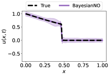
(a) In-domain

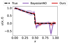
(b) OOD

,

Figure 1: 1-d Stefan Equation. In-domain (a) and OOD (b) predictions from FNO with post-hoc uncertainty estimates (3 standard deviations) obtained by BayesianNO (Magnani et al., 2022) at time $t=0.5$. The model outputs an accurate solution with reasonable uncertainty bounds in-domain (a), where the training and test input parameters are drawn from the same distribution, i.e., $u{{}^{*}}^{{\text{train}}},u{{}^{*}}^{{\text{test}}}\in[0.6,0.7]$. The model fails to do so when the test inputs are OOD (b), with $u{{}^{*}}^{{\text{test}}}\in[0.5,0.55]$. The large oscillation occurs at different locations for different seeds and we improve it.

To identify and correct OOD robustness issues, tools from regression diagnostics (Chatterjee & Hadi, 1988) and uncertainty quantification (UQ) (Schwaiger et al., 2020) may be used. Recent work (Magnani et al., 2022; Psaros et al., 2023) has shown that several UQ methods (Bayesian approaches, ensembles, variational methods) (Graves, 2011; Gal & Ghahramani, 2016; Lakshminarayanan et al., 2017; Teye et al., 2018; Yang et al., 2022) originally proposed for standard NNs provide well-calibrated uncertainty estimates for NOs when the test inputs are in-domain. In parallel with this, Hansen et al. (2023) proposed ProbConserv, a method to use well-calibrated uncertainty estimates to help constrain PDE solutions to satisfy conservation laws. A reliable UQ framework can offer valuable insights more generally: into sensitivity analysis; to identify regions with high sensitivities and study how perturbations (epistemic or aleatoric) impact the PDE solution (Xiu & Karniadakis, 2002; Le Maître & Knio, 2012; Rezaeiravesh et al., 2020); and potentially to enhance the accuracy and reliability of the original PDE method.

Problems with the existing UQ methods for NOs are that they either (i) fail to provide good uncertainty estimates for NOs for OOD predictions, or (ii) are computationally expensive, limiting the practical advantages of NOs over classical solvers. For example, Figure 1(a) shows that the Bayesian Neural Operator (BayesianNO) (Magnani et al., 2022) captures the associated uncertainty accurately for in-domain predictions, while Figure 1(b) shows that it is inaccurate for OOD tasks. This example shows that the uncertainty estimates from existing UQ methods may not be correlated with the prediction errors OOD, highlighting the need for improved UQ metrics and methods to detect this issue.

In this work, we address this challenge. We start by identifying failure modes of most existing UQ methods for NOs OOD, and we demonstrate that ensembling methods outperform other methods in this context, characterizing the benefits of the output diversity. However, ensembling can be expensive. Inspired by the success of ensembling, we propose DiverseNO, a method for scalable UQ for NOs that detects and reduces OOD prediction errors. Lastly, we use these uncertainty estimates within the recently-developed ProbConserv framework (Hansen et al., 2023) in Operator-ProbConserv, which further improves the OOD performance by satisfying known physical constraints of the problem. Our main contributions are as follows:

• We identify an important challenge when using NOs to solve PDE problems in practical OOD settings. In particular, we show that NOs fail to provide accurate solutions when test-time PDE parameters are outside the domain of the training data, even under mild domain shifts and when the model performs well in-domain. We also show that existing UQ methods for NOs (e.g., BayesianNO (Magnani et al., 2022)) that provide “good” in-domain uncertainty estimates fail to do so for OOD and/or are computationally very expensive. (See Section 3.1.)

• We demonstrate empirically that ensembles of NOs provide improved uncertainty estimates OOD, compared with existing UQ methods; and we identify diversity in the predictions of the individual models as the key reason for better OOD UQ. (See Section 3.2.)

• We propose DiverseNO, a simple cost-efficient alternative to ensembling that encourages diverse predictions (via regularization) to mimic the OOD properties of an ensemble. (See Section 4.1.)

• We use the error-correlated uncertainty estimates from DiverseNO as an input to the ProbConserv framework (Hansen et al., 2023). Our resulting Operator-ProbConserv uses the variance information to correct the prediction to satisfy known physical constraints, e.g., conservation laws. (See Section 4.2.)

• We provide an extensive empirical evaluation across a wide range of OOD PDE tasks that shows DiverseNO achieves $2\times$ to $70\times$ improvement in the meaningful UQ metric n-MeRCI compared to other computationally cheap UQ methods. Cost-performance tradeoff curves demonstrate its computational efficiency. We also show that using the uncertainty estimates from DiverseNO in Operator-ProbConserv further improves the OOD accuracy by up to $34\%$. (See Section 5.)

2 Background and Problem Setup

In this section, we introduce the basic problem, and we provide background on relevant UQ and sensitivity analysis.

2.1 Problem Definition

PDEs are used to describe the evolution of a physical quantity $u$ with respect to space and/or time. The general (differential) form of a PDE is given as:

$$\mathcal{F}_{\phi}u(x,t) =0,\qquad\forall x\in{\Omega},\forall t\in{[0,T]},$$

$$u(x,0) =u_{0}(x),\qquad\forall x\in{\Omega},$$

$${\mathcal{B}}u(x,t) =0,\qquad\forall x\in{\partial{\Omega}},\forall t\in{[0,T]},$$ (1)

where ${\Omega}\subseteq{\mathbb{R}}^{d}$ denotes a bounded domain with boundary ${\partial{\Omega}}$, $\mathcal{F}_{\phi}$ denotes a (potentially nonlinear) differential operator parameterized by $\phi:{\Omega}\to{\mathbb{R}}\in\Phi$ acting on the solution $u:{\Omega}\times{[0,T]}\to{\mathbb{R}}^{d_{o}},u\in\mathcal{U}$ for some final time $T$, $u_{0}:{\Omega}\to{\mathbb{R}}\in\mathcal{U}_{0}$ denotes the initial condition at time $t=0$, ${\mathcal{B}}$ denotes the boundary constraint operator; here $\Phi,\mathcal{U}_{0},\mathcal{U}$ denote appropriate Banach spaces. Our basic goal is to learn an operator ${A}:\Phi\to\mathcal{U}$ that accurately approximates the mapping from PDE parameters $\phi$ to the solution $u$. We consider $\phi\in\tilde{\Phi}\subseteq\Phi$ so that the problem defined in Section 2.1 is well-posed: it has a unique solution $u\in\mathcal{U}$ depending continuously on the input $\phi$ from $\tilde{\Phi}.$

Training distribution and data.

We assume that the operator ${A}$ is learned with an under-specified training distribution $\mathcal{H}^{\text{train}}(\phi)$, i.e., the support of $\mathcal{H}^{\text{train}}(\phi)$ does not cover the entire subspace $\tilde{\Phi}\subset\Phi$ of inputs for which the problem is well-posed. Samples from this distribution form our training data ${\mathcal{D}}^{\text{train}}=\{\phi^{(i)},u^{(i)}\}_{i=1}^{N}$, where $\phi^{(i)}\sim\mathcal{H}^{\text{train}}(\phi)$, $u^{(i)}={{A}^{\dagger}}(\phi^{(i)})$ and ${{A}^{\dagger}}$ denotes the ground-truth operator. Practically, discrete approximations of the functions $\phi^{(i)}$ and $u^{(i)}$ are evaluated at a given time $t$ (for time-dependent problems) on a grid $\{x_{l}\}_{l=1}^{L}\subset{\Omega}$, where $L$ denotes the number of gridpoints.

OOD test distribution.

We define the OOD task, where the learned operator is tested on inputs $\phi^{\text{test}}\sim\mathcal{H}^{\text{test}}(\phi)$ from the test distribution $\mathcal{H}^{\text{test}}(\phi)$, such that the ${\text{supp}}(\mathcal{H}^{\text{test}}(\phi))\neq{\text{supp}}(\mathcal{H}^{\text{train}}(\phi))$. We assume $\phi^{\text{test}}$ is evaluated on the same grid $\{x_{l}\}_{l=1}^{L}$ as during training.

2.2 Sensitivity Analysis for Operator Learning

When used with inputs close to the support of the training data, NOs can provide cost-efficient and accurate surrogates to augment traditional PDE solvers. Away from these inputs, however, it is important to be able to estimate potential uncertainties in the predictions made by the NO. Learning NN parameters has been viewed as a fully Bayesian problem (Teye et al., 2018; Magnani et al., 2022; Psarosa et al., 2022; Dandekar et al., 2022). To do this, one assumes a prior on the parameters, and then one adopts a statistical model to describe the generation of the training pairs and their relationship to the NN, defining the likelihood. Pursuing a fully Bayesian approach to learning the parameters of a NN is arguably unwise for (at least) three reasons: (i) it is computationally expensive; (ii) uncertainty in the parameters of the NO does not necessarily translate into uncertainty in outputs; and (iii) the model likelihood is likely to be mis-specified. (These are in addition to the fact that nontrivial issues arise when the NNs are overparameterized (Hodgkinson et al., 2022, 2023).) Viewing the problem through a Bayesian lens, even if not adopting a fully Bayesian approach, can be helpful. For example, using a Bayesian perspective, and the idea of collections of candidate solutions that match the data, facilitates the study of the sensitivities of learned NNs to perturbations of various kinds. In particular, for PDE operator learning, this approach has the potential to uncover regions of the physical domain which are most sensitive to perturbations resulting from deploying a NO outside the support of the training data.

We now describe the Bayesian model that we adopt. Consider the training data ${\mathcal{D}}^{\text{train}}=\{\phi^{(i)},u^{(i)}\}_{i=1}^{N}$ with $u^{(i)}:={{A}^{\dagger}}(\phi^{(i)})$. On the basis of this data, we attempt to learn the parameter ${\mathbf{\theta}}$ of a NO ${A}(\cdot;{\mathbf{\theta}})$ so that ${A}(\cdot;{\mathbf{\theta}})\approx{{A}^{\dagger}}(\cdot).$ To this end, we place the prior $p({\mathbf{\theta}})=\mathcal{N}({\mathbf{\theta}};{\bm{0}},\frac{1}{\alpha^{2}}{\mathbf{I}})$ on the parameters for some $\alpha\in\mathbb{R}$. We can assume that the training data is given by $u^{(i)}={A}(\phi^{(i)};{\mathbf{\theta}})+\eta,$ where $\eta$ denotes a mean zero Gaussian random variable with block-diagonal covariance, where the identity blocks are scaled, for each $i$, by the size of the ground truth operator, generating the data $\|{{A}^{\dagger}}(\phi^{(i)})\|_{2}^{2}.$ This model accounts for the fact that the training data is not actually drawn from a realization of the NN, and it leads to the likelihood

$$p(u^{(i)}|{\mathbf{\theta}},\phi^{(i)})=\mathcal{N}(u^{(i)};{A}(\phi^{(i)};{\mathbf{\theta}}),\frac{1}{\alpha^{2}}\|{{A}^{\dagger}}(\phi^{(i)})\|^{2}_{2}{\mathbf{I}}).\vspace{-0.2cm}$$

From Bayes Theorem, we obtain the posterior

$${p({\mathbf{\theta}}|{\mathcal{D}}^{\text{train}})}\propto\prod_{i=1}^{N}p(u^{(i)}|{\mathbf{\theta}},\phi^{(i)})p({\mathbf{\theta}}).\vspace{-0.2cm}$$ (2)

Estimating the exact posterior is intractable for most practical tasks. A common practice is to use the maximum a posteriori (MAP) estimate, ${\mathbf{\theta}}^{\text{MAP}}=\operatorname*{arg\,max}{p({\mathbf{\theta}}|{\mathcal{D}}^{\text{train}})}$, ignoring the uncertainty information and obtaining a single point prediction.

If an approximation of the ${p({\mathbf{\theta}}|{\mathcal{D}}^{\text{train}})}$ given in Equation 2 is known, then the probability distribution on output predictions $u^{\text{test}}$ from a test input $\phi^{\text{test}}$ can be obtained by the Bayesian model average (BMA),

$$p(u^{\text{test}}|\phi^{\text{test}},{\mathcal{D}}^{\text{train}})=\int_{\mathbf{\theta}}p(u^{\text{test}}|{\mathbf{\theta}},\phi^{\text{test}}){p({\mathbf{\theta}}|{\mathcal{D}}^{\text{train}})}d{\mathbf{\theta}}.\vspace{-0.2cm}$$ (3)

To capture the uncertainty in predictions, several approximate inference techniques have been proposed (Magnani et al., 2022; Lakshminarayanan et al., 2017; Graves, 2011; Teye et al., 2018; Gal & Ghahramani, 2016); these use a Monte Carlo approximation of Equation 3, i.e., $p(u^{\text{test}}|\phi^{\text{test}},{\mathcal{D}}^{\text{train}})\approx\frac{1}{J}\sum_{j=1}^{J}p(u^{\text{test}}|{\mathbf{\theta}}_{j},\phi^{\text{test}})$ with ${\mathbf{\theta}}_{j}\sim{p({\mathbf{\theta}}|{\mathcal{D}}^{\text{train}})}$, and they differ in the (approximate) procedure used to obtain samples ${\mathbf{\theta}}_{j}$ from the posterior. (See related work in Appendix A for details.)

Effect of training data underspecification.

A key difference between our OOD setting and the traditional setting is the under-specification of the training data, i.e., the support of $\mathcal{H}^{\text{train}}(\phi)$ does not cover the entire space $\tilde{\Phi}$. There are many NOs that can achieve close to zero training loss while disagreeing on OOD inputs. The posterior ${p({\mathbf{\theta}}|{\mathcal{D}}^{\text{train}})}$ has multiple modes, and choosing only one of these models can result in losing uncertainty information (regarding the predictions) that is important for the OOD test inputs.

There is a large body of work on numerical and SciML methods for solving PDEs, UQ for NOs, and diversity in ensembles; see Appendix A for a detailed discussion.

3 Do Existing Methods Give Good OOD UQ?

In this section, we use the 1-d heat equation as an illustrative example to evaluate existing UQ methods (Magnani et al., 2022; Lakshminarayanan et al., 2017; Gal & Ghahramani, 2016) with the aim of determining whether uncertainty estimates from these methods are robust to OOD shifts. We consider the Fourier Neural Operator (FNO) (Li et al., 2022a) as our base model, and we evaluate the OOD performance of several UQ methods. We show that EnsembleNO, which is based on DeepEnsembles in Lakshminarayanan et al. (2017), performs better than the other UQ methods OOD.

(a) BayesianNO

(b) VarianceNO

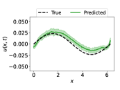
(c) MC-DropoutNO

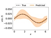
(d) EnsembleNO

Figure 2: 1-d Heat equation, large OOD shift. Uncertainty estimates (3 standard deviations) from various UQ methods under large OOD shifts in the input diffusivity coefficient, where $k^{\text{train}}\in[1,5],k^{\text{test}}\in[7,8]$. The EnsembleNO prediction, which is based on DeepEnsembles (Lakshminarayanan et al., 2017), is contained within its uncertainty estimate, whereas the predictions from the other methods have narrow uncertainty estimates and are inaccurate on this “easy” task.

3.1 OOD Failures of Existing UQ methods

While the existing UQ methods perform well in-domain (e.g., see BayesianNO in Figure 1(a)), we identify several canonical cases where they fail OOD. Figure 2 shows the solution profiles and uncertainty estimates to the 1-d heat equation for a large OOD shift, where $k^{{\text{train}}}\in[1,5]$ and $k^{{\text{test}}}\in[7,8]$. We see that the predictions are inaccurate for most of the UQ methods, with the solution not contained within the uncertainty estimate, other than for EnsembleNO. Quantitatively, we use the Normalized Mean Rescaled Confidence Interval (n-MeRCI) (Moukari et al., 2019) (defined formally in Equation 7 in Section 5), which measures how well the uncertainty estimates are correlated with the prediction errors, with lower values indicating better correlation. Surprisingly, EnsembleNO achieves significantly lower n-MeRCI value (e.g., 0.05 vs 0.8 in the heat equation) compared to the other UQ methods across various PDEs and OOD shifts. In contrast to the other UQ methods that output worse uncertainty estimates as the OOD shift increases, the ensemble model consistently outputs uncertainty estimates that are correlated with the prediction errors. (See Section B.1 for similar results on a range of PDEs.)

3.2 How do Ensembles Provide Better OOD UQ

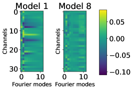
(a) Heatmaps of first Fourier layer weights of two diverse FNO models.

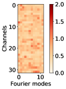
(b) Coefficient of variation (std/mean) of the first Fourier layer weights

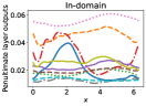
(c) ID penultimate layer

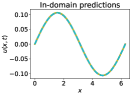
(d) ID predictions

(e) OOD penultimate layer

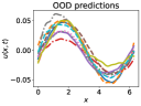
(f) OOD predictions

Figure 3: Diversity of Models in an Ensemble of NOs (EnsembleNO). (a) Heatmaps of the weights, (b) coefficient of variation of the 10 models in the ensemble, and (c-f) penultimate and last layer outputs on a 1-d heat equation task. (c-d) For in-domain (ID) input, the last layer removes the diversity from the intermediate outputs and maps the final output close to the ground truth. (e-f) For OOD input, this diversity remains in the output.

In this subsection, we study the reason behind significantly better OOD uncertainty estimates from a seemingly simple ensemble of NOs i.e., EnsembleNO. Wilson & Izmailov (2020) posit that ensembles are able to explore the different modes of the posterior better than other UQ methods that use, e.g., variational inference or a Laplace approximation, since these methods are only able to explore a single posterior mode due to the Gaussian assumption. They show that samples of weights ${\mathbf{\theta}}_{j}$ from a single posterior mode are not functionally very diverse, i.e., the corresponding predictions from these models ${A}(\cdot;{\mathbf{\theta}}_{j})$ are not very different from each other. This leads to a suboptimal estimation of the BMA in Equation 3, as the Monte Carlo sum contains redundant terms. In contrast, individual models of the ensembles reach distinct posterior modes due to the random initialization and the noise in SGD training. The resulting functional diversity allows the ensemble to better estimate Equation 3. Next, we show that this diversity with the models in the ensemble holds empirically for operator learning as well.

In Figure 3, we illustrate the diversity in operator learning by visualizing the differences in the Fourier layer weights and final layer outputs for the models in the ensemble on a 1-d heat equation task. (See Section B.2 for analogous results across a variety of PDEs and Fourier layers.) Different models seem to focus on different spectral characteristics of its input function. For example, the heatmaps of the weights in Figure 3(a) show that the first model (left) uses the low-frequency components across most channels except a few, whereas another model (right) uses the available Fourier components across all the channels. Figure 3(b) illustrates that this model diversity holds for all models in the ensemble since the coefficient of variation of the Fourier layer weights computed across the ten models is large.

The intermediate outputs from the different models in the ensemble also show diversity in operator learning until the last layer with a key difference between the in-domain and OOD final outputs. Given the same in-domain input, the first feed-forward (lifting) layer of these models already produces diverse outputs which continues until the penultimate layer (Figure 3(c)). Figure 3(d) shows that the last layer removes the diversity and maps the outputs to the same ground truth for an in-domain input. Figures 3(e) and 3(f) illustrates that a different trend occurs for an OOD input. The OOD intermediate outputs are also diverse, the difference here is that this diversity does not vanish from the last layer outputs since the model is not able to match the ground truth data. This representative example demonstrates how the ensemble model captures epistemic uncertainty in the OOD setting. We see that the individual models in the ensemble fit the training data with close to zero error, but are diverse and disagree for OOD inputs. Ensembles can approximate the BMA in Equation 3 with functionally diverse models from the posterior, leading to better OOD uncertainty estimates.

4 DiverseNO + ProbConserv

In this section, we first present our DiverseNO model, which encourages diverse OOD predictions, while being significantly computationally cheaper than EnsembleNO (Lakshminarayanan et al., 2017). We then feed these black-box NO uncertainty estimates into the first step of the probabilistic ProbConserv framework (Hansen et al., 2023) to enforce physical constraints and further improve the OOD model performance. As opposed to in ProbConserv, here the constraint is applied on the OOD predictions.

4.1 DiverseNO: Computationally Efficient OOD UQ

The primary challenge with ensembles is their high computational complexity during both training and inference. An ensemble-based model for surrogate modeling diminishes the computational benefits gained from using a data-driven approach over classical solvers. Here, we propose DiverseNO, a method which makes a simple modification to the NO architecture, along with a diversity-enforcing regularization term, to emulate the favorable UQ properties of EnsembleNO, while being computationally cheaper.

For the architecture change, we modify the last feed-forward layer to have $M$ output/prediction heads instead of one. The architecture may be viewed as an ensemble with the individual models sharing parameters up to the penultimate layer. While parameter-sharing significantly reduces the computational complexity, when compared to using a full ensemble, it simultaneously hinders the diversity within the ensemble, which we showed is a crucial element for generating good uncertainty estimates. (See Section 3.2.)

To mitigate this, and to encourage diverse predictions, we propose to maximize the following diversity measure among the last-layer weights corresponding to the $M$ prediction heads. We also constrain the in-domain predictions from each of these heads to match the ground truth outputs. Formally, we solve:

$$\hat{{\mathbf{\theta}}}=\operatorname*{arg\,min}_{{\mathbf{\theta}}}\underbrace{\frac{1}{NM}\sum_{i=1}^{N}\sum_{m=1}^{M}{\frac{||\hat{u}_{m}^{(i)}-u^{(i)}||^{2}_{L_{2}}}{||u^{(i)}||^{2}_{L_{2}}}}}_{\text{unconstrained NO loss}}\underbrace{-\frac{2\lambda_{\text{diverse}}}{M(M-1)}\sum_{m,k:m<k}||{\mathbf{\theta}}_{m}-{\mathbf{\theta}}_{k}||^{2}_{2}}_{\text{diversity regularization}},$$ (4)

where ${\mathbf{\theta}}_{m}$ and ${\mathbf{\theta}}_{k}$ denote the last-layer weights corresponding to $m$-th and $k$-th prediction heads, respectively, $\hat{u}_{m}^{(i)}$ denotes the prediction from $m$-th output head for the $i$-th training example, and $u^{(i)}$ denotes the corresponding ground truth. The first term in Equation 4 is the relative $L_{2}$ loss standard in NO training. We add the regularizing second term to encourage diversity in the last-layer weights corresponding to the different head. The hyperparameter $\lambda_{\text{diverse}}$ controls the strength of the diversity regularization relative to the prediction loss. A naive selection procedure for $\lambda_{\text{diverse}}$ using only in-domain validation MSE selects an unconstrained model with no diversity penalty. Instead, we select the maximum regularization strength $\lambda_{\text{diverse}}$ that achieves an in-domain validation MSE within 10% of the identified best in-domain validation MSE. 10% is an arbitrary tolerance that denotes the % accuracy the practitioner is willing to forego to achieve better OOD UQ. This procedure trades off in-domain prediction errors for higher diversity that is useful for OOD UQ. See Appendix C for ablations with regularizations for ensemble NNs that directly diversify the predictions (Bourel et al., 2020; Zhang et al., 2020).

4.2 Operator-ProbConserv

We detail how to use uncertainty estimates for NOs, e.g., DiverseNO, within the ProbConserv framework (Hansen et al., 2023) to improve OOD performance and incorporate physical constraints known to be satisfied by the PDEs we consider.

The two-step procedure is given as:

1. Compute uncertainty estimates $\mu,\Sigma$ from the NO;

2. Use the update rule from ProbConserv, described in Equation 6 below, to improve to the model.

Given the predictions $\mu$ and the covariance matrix $\Sigma$, ProbConserv solves the constrained least squares problem:

$$\tilde{\mu}=\operatorname*{arg\,min}_{y}\frac{1}{2}||y-\mu||^{2}_{\Sigma^{-1}}\quad\text{s.t.}\quad Gy=b,$$ (5)

where $G$ denotes the constraint matrix. For example, conservation of mass in the 1-d heat equation with zero Dirichlet boundary conditions is given by the linear constraint $\int_{x}u(x,t)dx=0$ and $G$ can take the form of a discretized integral. The optimization in Equation 5 can be solved in closed form with the following update:

$$\tilde{\mu} =\mu-\Sigma G^{T}(G\Sigma G^{T})^{-1}(G\mu-b),$$ (6a)

$$\tilde{\Sigma} =\Sigma-\Sigma G^{T}(G\Sigma G^{T})^{-1}G\Sigma.$$ (6b)

For the UQ methods for NOs considered here, $\Sigma$ denotes a diagonal matrix with the variance estimates on the diagonal. The update can be viewed as an oblique projection of the unconstrained predictions $\mu$ onto the constrained subspace, while taking into account the variance (via $\Sigma$) in the predictions. When the uncertainty estimates are not uniform, ProbConserv encourages higher corrections in regions of higher variance, and it is important to have uncertainty estimates that are correlated with the prediction errors.

In the original implementation of ProbConserv (Hansen et al., 2023), the Attentive Neural Process (ANP) (Kim et al., 2019) is used as an instantiation of the framework in ProbConserv-ANP. There has yet to be an operator model, which is typically more suitable for SciML problems, used within ProbConserv. We show its effectiveness with NO uncertainty estimates and its application to OOD tasks.

5 Empirical Results

In this section, we evaluate DiverseNO against several baselines for using UQ in PDE solving, with a specific aim to answer the following questions:

1. Is diversity in the weights of the last layer of DiverseNO enough to obtain good uncertainty estimates? (See Section 5.1.)

2. What are the computational savings of DiverseNO compared to ensembling? (See Section 5.2.)

3. Does using error-correlated UQ in ProbConserv help improve OOD prediction errors in PDE tasks? (See Section 5.3.)

Uncertainty metrics.

Several metrics have been used to evaluate the goodness of uncertainty estimates, e.g., negative log-likelihood (NLL), root mean squared calibration error (RMSCE), sharpness and continuous ranked probability score (CRPS) (Gneiting et al., 2007; Gneiting & Raftery, 2007; Kuleshov et al., 2018; Psaros et al., 2023). We use the normalized Mean Rescaled Confidence Interval (n-MeRCI) metric (Moukari et al., 2019), that evaluates how well the uncertainty estimates are correlated with the prediction errors. The n-MeRCI metric is given as:

$$\text{n-MeRCI}=\frac{\frac{1}{N}\sum_{i=1}^{N}\tau\sigma_{i}-\text{MAE}}{\max(|\hat{u}_{i}-u_{i}|)-\text{MAE}},$$ (7)

where MAE denotes the mean absolute error and $\tau$ denotes the 95${}^{\text{th}}$ percentile of the ratios $|\hat{u}_{i}-u_{i}|/\sigma_{i}$. This percentile of the ratios scales the uncertainty estimates so that the measure is scale-independent and robust to outliers. Values closer to zero correspond to better-correlated uncertainty estimates, whereas values closer to one or greater correspond to uncorrelated/random estimates. See Section F.1 for the MSE, NLL, RMSCE and CRPS metrics.

Baselines.

We use the Fourier Neural Operator (FNO) (Li et al., 2022a) as a base model and leave similar investigations of other operators to future work. To provide uncertainty estimates in PDE applications, we compare our proposed UQ method, DiverseNO, with the following four commonly-used baselines of approximate Bayesian inference (Psaros et al., 2023): (i) BayesianNO (Magnani et al., 2022), that uses the (last-layer) Laplace approximation over the MAP estimate to approximate the posterior; (ii) VarianceNO (Lakshminarayanan et al., 2017), which outputs the mean and variance and which is trained with the negative log-likelihood; (iii) MC-DropoutNO (Gal & Ghahramani, 2016), where dropout in the feed-forward layers is used as approximate variational inference; and (iv) EnsembleNO (Lakshminarayanan et al., 2017), where we train $K$ randomly initialized FNO models (in our experiments, $K=10$) and compute the empirical mean and variance of the predictions.

GPME Benchmarking Family of Equations.

The Generalized Porous Medium Equation (GPME) is a family of PDEs parameterized by a (potentially nonlinear) coefficient $k(u)$  (Maddix et al., 2018a, b). The GPME models fluid flow through a porous medium, and it has additional applications in heat transfer, groundwater flow, and crystallization, to name a few (Vázquez, 2007). It can be written in the conservative form with flux $F(u)=-k(u)\nabla u$ as:

$$u_{t}-\nabla\cdot(k(u)\nabla u)=0,\qquad x\in\Omega,t\in{[0,T]},$$ (8)

where $k(u):{\Omega}\to{\mathbb{R}}$ denotes the diffusion coefficient. We consider three instances of the GPME on a 1-d domain ${\Omega}=[0,S]$. By varying $k(u)$, these correspond to increasing levels of difficulty (Hansen et al., 2023): (i) an “easy” case, with $k(u)=k$, the standard heat equation (linear, constant coefficient, parabolic); (ii) a “medium” case, with $k(u)=u^{m},m\geq 1$, the Porous Medium Equation (PME) (nonlinear, degenerate parabolic); and (iii) a “hard” case, with $k(u)={\bm{1}}_{u\geq u^{*}},u^{*}>0$, the Stefan problem (nonlinear, discontinuous, degenerate parabolic).

We aim to learn an operator that maps the constant parameter $c$ identifying the diffusion coefficient $k(u)$—constant $k$ in the heat equation, degree $m$ in the PME, and $u^{*}$ in the Stefan equation—to the solution $u(\cdot,T)$ for some $T>0$. Input to the NO is a constant scalar field taking the value $c$ for all spatiotemporal points. Our training dataset consists of $N=400$ input/output pairs $\{\phi^{(i)},u^{(i)}\}_{i=1}^{N}$, where $\phi^{(i)}(x,t):=c^{(i)}$ denotes a constant function identifying the diffusion coefficient with value $c^{(i)}$ over the domain and $u^{(i)}$ denotes the corresponding solutions at discrete times $t\in[0,T]$. We keep the initial and boundary conditions fixed for all the examples of a particular PDE. During training, we sample the constant parameter $c^{(i)}\sim\mathcal{H}^{\text{train}}(c)$ and we evaluate the trained neural operator on OOD shifts $c^{(i)}\sim\mathcal{H}^{\text{test}}(c)$, where $\mathcal{H}^{\text{test}}(c)$ has no support overlap with $\mathcal{H}^{\text{train}}(c)$. We consider small, medium and large OOD shifts for each PDE task based on the distance between $\mathcal{H}^{\text{train}}(c)$ and $\mathcal{H}^{\text{test}}(c)$. See Appendix D for details about the PDE test problems and Appendix E for additional experimental settings.

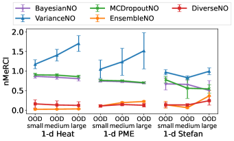
Figure 4: Performance vs. OOD shift. n-MeRCI $\downarrow$ of the UQ methods with increasing OOD shifts in the “easy,” “medium,” and “hard” cases of the GPME. EnsembleNO and DiverseNO consistently achieve low n-MeRCI values, indicating higher correlation between their uncertainty estimates and prediction errors.

5.1 Uncertainty estimates from DiverseNO

In Section 3, we showed that EnsembleNO outputs better uncertainty estimates OOD due to the diversity in the predictions among each model in the ensemble. Here, we evaluate whether DiverseNO can output good uncertainty estimates due to the diversity enforced over the last layer alone. Figure 4 shows the n-MeRCI metric for all UQ methods on increasing OOD shifts on the “easy”, ”medium” and “hard” cases of GPME. DiverseNO consistently outperforms BayesianNO, VarianceNO and MC-DropoutNO by $2\times$ to $70\times$ across all PDEs and OOD shifts, and is comparable (sometimes better) to the more expensive EnsembleNO that has diversity in weights of all layers (as seen in Figure 3). The n-MeRCI metric is generally close to zero for both methods indicating that their uncertainty estimates are well-correlated with the prediction errors and can be used to detect OOD shifts. See Section F.1 for additional metrics, solution profiles and uncertainty estimates.

5.2 Computational savings from DiverseNO

Figure 5 shows the computational savings of DiverseNO compared to EnsembleNO on the PME task with medium OOD shift, i.e., $m^{\text{train}}\in[2,3],m^{\text{test}}\in[4,5]$. We plot the MSE and n-MeRCI metric as a function of the number of floating point operations (FLOPs) for different model sizes (using the derivation of FLOPs for FNO by de Hoop et al. (2022)). We see that DiverseNO is significantly more efficient across the various PDEs: for similar number of FLOPs, DiverseNO is 49% to 80% better in MSE and comparable to EnsembleNO in the n-MeRCI metric. (See Section F.2 for the cost performance curves as a function of the number of parameters.)

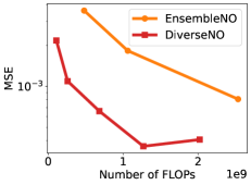
(a) MSE $\downarrow$

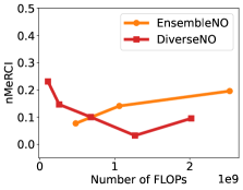
(b) n-MeRCI $\downarrow$

Figure 5: Cost-performance tradeoff. MSE $\downarrow$ and n-MeRCI $\downarrow$ vs. the number of floating point operations (FLOPs) for EnsembleNO and DiverseNO with varying number of parameters on the PME task with medium OOD shift, i.e., $m^{\text{train}}\in[2,3],m^{\text{test}}\in[4,5]$.

5.3 OOD applications of UQ with ProbConserv

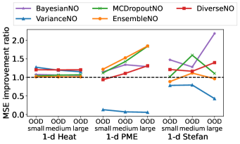
Figure 6: MSE Improvement Ratio for ProbConserv. The MSE ratio before and after applying ProbConserv to the UQ methods ($\geq 1$ indicates improvement) for increasing OOD shifts in the “easy”, “medium” and “hard” cases of the GPME.

We investigate whether uncertainty estimates obtained from the UQ methods can be used to improve OOD performance and to apply probabilistic physics-based constraints. We use ProbConserv (Hansen et al., 2023) to enforce a known linear conservation constraint of the form $\int_{x}u(x,t)dx=b(t)$ corresponding to each of the PDEs considered. (See Section 4.2.) When applying ProbConserv, we use the discretized form of the constraint $Gu=b+\sigma_{G}\epsilon$, where $\epsilon$ denotes a noise term that allows for a slack in the constraint for practical considerations. We use $\sigma_{G}=10^{-9}$ in our experiments. We report the conservation errors (CE) in Section F.3 and show that conservation is typically violated OOD for the unconstrained NO methods (with CE $\approx\!10^{-2}$ for the heat equation, $\approx\!0.3$ for PME and $\approx\!0.4$ for Stefan) and ProbConserv enforces the known physical constraint exactly for all UQ methods (i.e., with $\text{CE}=0$).

Figure 6 shows the MSE ratio before and after applying ProbConserv (larger than 1 indicates improvement) for all 3 PDEs and OOD shifts. (See Section F.3 for the exact metrics.) Similar to the original ProbConserv (Hansen et al., 2023) work for in-domain problems, we also observe differing behaviors of applying ProbConserv on “easy” to “hard” PDEs for OOD problems. In the “easy” heat equation, ProbConserv improves OOD MSE for all the UQ methods, even when the uncertainty estimates are uncalibrated (e.g., for VarianceNO). DiverseNO improves the most with ProbConserv ($1.4\times$) and subsequently achieves the lowest MSE of all methods in every OOD shift ($1.8\times$ to $5.5\times$ better than baselines). For “medium” and “hard” cases of GPME, the effect of ProbConserv depends on the goodness of uncertainty estimates. For instance, ProbConserv degrades the performance of VarianceNO drastically (by 1300% and 31% for small OOD shifts in the 2 PDEs) because of uncalibrated uncertainty estimates. Figure 7(a) supports a similar finding for BayesianNO in the “hard” Stefan case: ProbConserv is not able to correct the oscillation near the right boundary since the corresponding uncertainty estimates are much lower. In contrast, ProbConserv fixes these oscillations for DiverseNO (Figure 7(b)). These findings demonstrate the need for uncertainty estimates that are correlated with prediction errors. Finally, for large OOD shifts in the “medium”/“hard” PDEs, prediction errors remain high for all methods ($\approx\!10^{-2}$) after applying ProbConserv, indicating that global conservation constraint alone is not enough to solve these challenging OOD tasks and additional (local) physical constraints may be required. Overall, we show that with error-correlated UQ from DiverseNO, ProbConserv can be effective against small to medium OOD shifts.

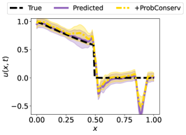
(a) BayesianNO +
ProbConserv

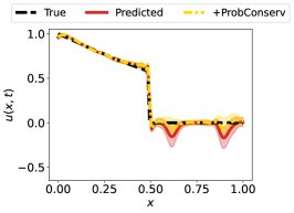
(b) DiverseNO + ProbConserv

Figure 7: Effect of ProbConserv update. Solution profiles before and after applying ProbConserv over DiverseNO and BayesianNO on 1-d Stefan with small OOD shift. (a) ProbConserv is able to correct the dips in DiverseNO’s solution as the uncertainty estimates are high in those regions as well. (b) Uncertainty estimates from BayesianNO are not correlated with the errors and ProbConserv focuses on $x=0.4$ where the solution was already accurate instead of the dip at $x=0.9$.

6 Conclusion

NOs have proven to be a successful class of data-driven methods for efficiently approximating the solution to certain PDE problems on in-domain tasks. In this work, we have shown that, despite these promising initial successes, NOs are not robust to OOD shifts in their inputs, in particular to shifts in PDE parameters. We show that a computationally-expensive ensemble of NOs provides a strong baseline for good OOD uncertainty estimates; and, motivated by this, we propose a simple scalable alternative, DiverseNO, that provides uncertainty estimates that are well-correlated with prediction errors. We use these error-correlated uncertainty estimates from DiverseNO within the ProbConserv framework (Hansen et al., 2023) to develop Operator-ProbConserv. We show that having UQ estimates that are well-correlated with the error are critical for the success of Operator-ProbConserv in improving the OOD performance. Our empirical results demonstrate that Operator-ProbConserv improves the accuracy of NOs across a wide range of PDE problem settings, in particular in high-error regions of the spatial domain. The improvements are particularly prominent on problems with shocks and that satisfy conservation laws. Future work includes extending Operator-ProbConserv to perform updates locally in the areas with the highest error estimates and to further improve and characterize the need for the well-correlated UQ estimates with the error.

Appendix A Related Work

Numerical methods. PDEs are ubiquitous throughout science and engineering, where they are used to model the evolution of various physical phenomena. These equations are typically solved for different values of PDE physical parameters, e.g., diffusivity in the heat equation, wavespeed in the advection equation, and the Reynolds number in Navier-Stokes equations. Solving PDEs typically requires extensive numerical knowledge and computational effort. Traditional approaches to solve PDEs (e.g., finite difference LeVeque (2007), finite volume LeVeque (2002) and finite element Hughes (2000) methods) can be computationally expensive, as their accuracy is dependent on the level of discretization of the spatial and temporal domains. Finer meshes are required to achieve high accuracy, resulting in increased computational costs. In addition, these approaches require a full re-run from scratch whenever there are changes in PDE parameters, which may not be known a priori.

SciML works on solving PDEs.

To alleviate the drawbacks of numerical methods, recent works in scientific machine learning (SciML) propose to use data-driven approaches to solve PDEs. These include so-called Physics-informed Neural Networks (PINNs) (Raissi et al., 2019), NOs (Li et al., 2020a, 2022b; Lu et al., 2019; Gupta et al., 2021; Yin et al., 2022), and reduced-order models for discovery (Brunton et al., 2016; Conti et al., 2023). By now, it has been shown that PINNs have several fundamental challenges associated with its soft constraint approach. In particular, it solves a single instance of the PDE with a fixed set of PDE parameters, is challenging to optimize for PDEs with large parameter values (Krishnapriyan et al., 2021; Edwards, 2022); and may return trivial solutions (Leiteritz & Pflüger, 2021). On the other hand, NOs (Kovachki et al., 2021; Li et al., 2020a) enjoy appealing properties of discretization invariance and universal approximation, while also achieving low approximation errors on in-domain tasks. Being purely data-driven, they are not guaranteed to satisfy all the physical properties of the solution. To address this, existing work has tried to incorporate different physical constraints via regularization (Li et al., 2021), within the architecture (e.g., boundary constraints in Saad et al. (2023), invariance in Liu et al. (2023), and PDE hard constraints in Négiar et al. (2023)) or via a projection to enforce conservation laws in Hansen et al. (2023). Most of these methods do not address the OOD problem that can occur even after enforcing these constraints. Subramanian et al. (2023) show that fine-tuning FNO models on OOD data is typically required to achieve reasonable performance. In particular, for significant OOD shifts, few-shot transfer learning requires a large amount of fine-tuning OOD data that may be unavailable for certain applications. Benitez et al. (2023) propose a variant of FNO specifically designed to learn the wavespeed to solution mapping in the Helmholtz equation and show that it performs better OOD.

UQ for Neural Operators.

Several Bayesian deep learning methods common for standard neural networks have been shown to work well for NOs on in-domain PDE applications (Psaros et al., 2023; Zou et al., 2023). Commonly used methodologies for approximate Bayesian inference, e.g., the Bayesian Neural Operator (Magnani et al., 2022), DeepEnsembles (Lakshminarayanan et al., 2017), variational inference methods, e.g., Mean-field VI  (Graves, 2011; Teye et al., 2018) or MC-Dropout  (Gal & Ghahramani, 2016) and MCMC approaches, e.g., Hamiltonian Monte Carlo (HMC), provide, at best, crude approximations of the true posterior distribution in Equation 3 of this Bayesian model. For instance, DeepEnsembles train the same architecture multiple times to obtain different models that maximize the posterior, i.e., different modes of the posterior. The Bayesian Neural Operator uses a Laplace approximation of the posterior. Variational inference approaches approximate the posterior with a density $q({\mathbf{\theta}})$, and sample ${\mathbf{\theta}}_{j}\sim q({\mathbf{\theta}})$. MCMC methods construct a Markov chain that is asymptotically guaranteed to sample from the true posterior. While these methods can provide good in-domain uncertainty estimates, most of the scalable UQ methods are not robust to OOD shifts.

Diversity in Ensembles.

There are several works that study the importance of diversity in ensemble-based approaches. Theisen et al. (2023) show that disagreement is key for an ensemble to be effective (with respect to accuracy). Wood et al. (2023) study the role of diversity in reducing in-domain generalization error. Diversity measures directly diversify the outputs from the different models in the ensemble, e.g., via minimizing the mutual information for classification tasks (Lee et al., 2022; Sinha et al., 2020; Rame & Cord, 2021), or the $L_{2}$ distance between the outputs for regression tasks. A recent work, DivDis (Lee et al., 2022) is the most related to our work in that it uses multiple prediction heads with diverse outputs to improve OOD accuracy in classification tasks. In particular, DivDis minimizes the mutual information between the outputs from different prediction heads when given OOD inputs (assumed to be known during training). This differs from our work since in operator learning, diversifying outputs directly does not provide informative uncertainty estimates.

Appendix B Advantages of Diversity in Ensembling on a Range of PDEs

In this section, we show that EnsembleNO performs well on a wide range of 1-d PDEs including the (degenerate) parabolic GPME family and the linear advection hyperbolic conservation law. We then show the corresponding heatmaps of the weights for each of the FNO models in the ensemble. This diversity is present in the ensemble across these PDEs and various Fourier layers, which motivates our development in enforcing diversity in DiverseNO.

B.1 Good Performance of Ensembling across Various PDEs and OOD Shifts

Figure 8 illustrates the strong performance of the ensemble compared to various UQ baselines across the GPME benchmarking family of PDEs with increasing difficulty and increasing OOD shifts. Figure 8(a) shows that the MSE increases for all methods as the problem difficulty and shift increases. Figure 8(b) shows that EnsembleNO performs significantly better than the baselines with respect to the n-MeRCI metric with close to zero values, indicating that the uncertainty estimates are well-correlated with the prediction error.

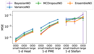
(a) MSE

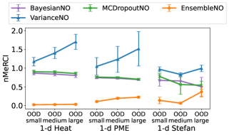
(b) n-MeRCI

Figure 8: MSE $\downarrow$ and n-MeRCI $\downarrow$ metrics for all UQ methods on GPME family of PDEs under small, medium and large OOD shifts. (a) MSE increases for all methods with increasing OOD shift and increasing PDE difficulty. (b) EnsembleNO performs significantly better in the n-MeRCI metric compared to other UQ baselines, with generally close to zero values, indicating that its uncertainty estimates are most correlated with prediction errors.

B.2 Diversity in the Heatmaps of the Ensemble

Figures 9-16 illustrate the diversity in each FNO model in the ensemble across a wide variety of PDEs with various levels of difficulty and various Fourier layers. In each figure, (a) shows the heatmaps of the weights in the corresponding Fourier layer across the channels and Fourier modes. This apparent diversity is reinforced in (b), which plots the coefficient of variation, i.e., the (mean/std) across all the models in the ensemble across the channels and Fourier modes.

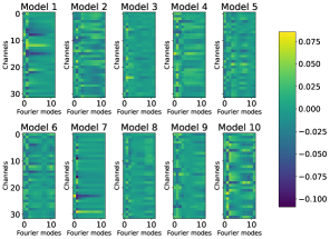
(a) Heatmaps of the first Fourier layer weights from an ensemble of 10 FNO models.

(b) Coefficient of variation (mean/std) of the first Fourier layer weights across the 10 models in the ensemble.

Figure 9: First Fourier layer of FNO models trained on 1-d heat equation task with $k^{\text{train}}\in[1,5]$.

(a) Heatmaps of the last Fourier layer weights from an ensemble of 10 FNO models.

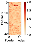
(b) Coefficient of variation (mean/std) of the last Fourier layer weights across the 10 models in the ensemble.

Figure 10: Last Fourier layer of FNO models trained on 1-d heat equation task with $k^{\text{train}}\in[1,5]$.

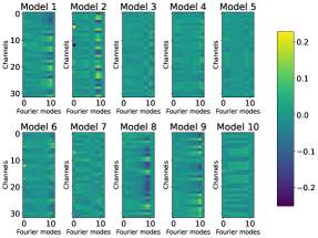
(a) Heatmaps of the first Fourier layer weights from an ensemble of 10 FNO models.

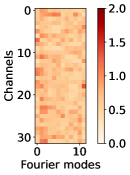
(b) Coefficient of variation (mean/std) of the first Fourier layer weights across the 10 models in the ensemble.

Figure 11: First Fourier layer of FNO models trained on 1-d PME task with $m^{\text{train}}\in[2,3]$.

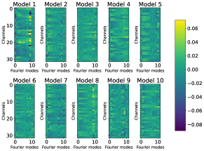
(a) Heatmaps of the last Fourier layer weights from an ensemble of 10 FNO models.

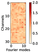
(b) Coefficient of variation (mean/std) of the last Fourier layer weights across the 10 models in the ensemble.

Figure 12: Last Fourier layer of FNO models trained on 1-d PME task with $m^{\text{train}}\in[2,3]$.

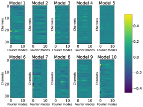
(a) Heatmaps of first Fourier layer weights from an ensemble of 10 FNO models.

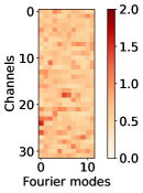
(b) Coefficient of variation (mean/std) of the first Fourier layer weights across the 10 models in the ensemble.

Figure 13: First Fourier layer of FNO models trained on 1-d Stefan task with $u^{*,{\text{train}}}\in[0.6,0.65]$.

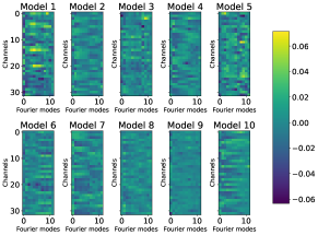
(a) Heatmaps of the last Fourier layer weights from an ensemble of 10 FNO models.

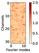
(b) Coefficient of variation (mean/std) of the last Fourier layer weights across the 10 models in the ensemble.

Figure 14: Last Fourier layer of FNO models trained on 1-d Stefan task with $u^{*,{\text{train}}}\in[0.6,0.65]$.

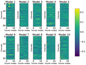
(a) Heatmaps of first Fourier layer weights from an ensemble of 10 FNO models.

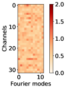
(b) Coefficient of variation (mean/std) of the first Fourier layer weights across the 10 models in the ensemble.

Figure 15: First Fourier layer of FNO models trained on 1-d linear advection task with $\beta^{\text{train}}\in[1,2]$.

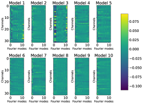
(a) Heatmaps of the last Fourier layer weights from an ensemble of 10 FNO models.

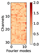
(b) Coefficient of variation (mean/std) of the last Fourier layer weights across the 10 models in the ensemble.

Figure 16: Last Fourier layer of FNO models trained on 1-d linear advection task with $\beta^{\text{train}}\in[1,2]$.

Appendix C Diversity Regularization Ablations

In our proposed DiverseNO, we solve the optimization problem in Equation 4. We test different regularizations in the second term of Equation 4 to enforce diversity in the last layer heads of DiverseNO: maximize the $L_{2}$ loss between (a) the weights of each head (ours), (b) the OOD predictions of each head, and (c) the gradients with respect to each head. For (b) and (c), we try two variants: the $L_{2}$ between the respective quantities after standardizing them to have mean 0 and variance 1, and without standardization. Note that (b) requires access to a set of OOD inputs without corresponding target outputs. Figures 17 -18 show that the proposed diversity measure results in best MSE and n-MeRCI performance across all OOD shifts. Regularizations that directly diversify the outputs or gradients are also sensitive to the regularization strength and require a careful trade-off between the prediction loss and regularization penalty. Proposed regularization is more robust to the hyperparameter and monotonically improves the performance for reasonable values of regularization strength.

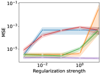
(a) Small OOD shift

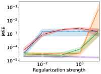
(b) Medium OOD shift

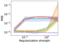
(c) Large OOD shift

Figure 17: Diversity regularization ablation. Effect of different diversity regularizations on MSE for small, medium, large OOD shifts in the 1-d heat equation. Our proposed regularization of enforcing diversity over the weights of each head has the best performance across various regularization strengths and OOD shifts.

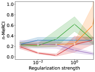
(a) Small OOD shift

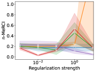
(b) Medium OOD shift

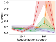
(c) Large OOD shift

Figure 18: Diversity regularization ablation. Effect of different diversity regularizations on n-MeRCI for small, medium, large OOD shifts in the 1-d heat equation. Our proposed regularization of enforcing diversity over the weights of each head has the best performance across various regularization strengths and OOD shifts.

Appendix D PDE Test Problems

In this section, we provide the details of the various test problems that we study, and the construction of both the training and test OOD datasets (See Table 1 for a summary).

D.1 Generalized Porous Medium Equation (GPME) Family

The Generalized Porous Medium Equation (GPME) is a family of PDEs parameterized by a (potentially nonlinear) coefficient $k(u)$  Maddix et al. (2018a, b). The GPME models fluid flow through a porous medium, and it has additional applications in heat transfer, groundwater flow, and crystallization, to name a few (Vázquez, 2007). It can be written in the conservative form with flux $F(u)=-k(u)\nabla u$ as:

$$u_{t}-\nabla\cdot(k(u)\nabla u)=0,\qquad x\in\Omega,t\in{[0,T]},$$ (9)

where $k(u):{\Omega}\to{\mathbb{R}}$ denotes the (potentially nonlinear) diffusion coefficient. We consider three instances of the GPME with increasing levels of difficulty by varying $k(u)$ (Hansen et al., 2023): (i) “easy” case with $k(u)=k$, the standard heat equation (linear, constant coefficient parabolic and smooth); (ii) “medium” case with $k(u)=u^{m},m\geq 1$, the Porous Medium Equation (PME) (nonlinear, degenerate parabolic); and (iii) “hard” case with $k(u)={\bm{1}}_{u\geq u^{*}},u^{*}>0$, the Stefan problem (nonlinear, degenerate parabolic with shock).

Table 1: Shows the parameter ranges for training and different OOD tasks corresponding to the four tested PDEs. For each PDE, we train the models on a range of parameter inputs (e.g., $k^{\text{train}}\in[1,5]$ for heat equation) and test on increasing OOD shifts (e.g., $k^{\text{test}}\in[5,6]$ for a small shift in heat equation).

PDE	Task	Parameter range
Heat Equation	Train	$k\in[1,5]$
$u_{t}-\nabla\cdot(k\nabla u)=0$	OOD small	$k\in[5,6]$
	OOD medium	$k\in[6,7]$
	OOD large	$k\in[7,8]$
Porous Medium Equation (PME)	Train	$m\in[2,3]$
$u_{t}-\nabla\cdot(u^{m}\nabla u)=0$	OOD small	$m\in[1,2]$
	OOD medium	$m\in[4,5]$
	OOD large	$m\in[5,6]$
Stefan Equation	Train	$u^{*}\in[0.6,0.65]$
$u_{t}-\nabla\cdot({\bm{1}}_{u\geq u^{*}}\nabla u)=0$	OOD small	$u^{*}\in[0.55,0.6]$
	OOD medium	$u^{*}\in[0.7,0.75]$
	OOD large	$u^{*}\in[0.5,0.55]$
Linear advection	Train	$\beta\in[1,~{}~{}2]$
$u_{t}+\beta u_{x}=0$	OOD small	$\beta\in[0.5,1]$
	OOD medium	$\beta\in[2.5,3]$
	OOD large	$\beta\in[3,3.5]$

D.1.1 Heat (Diffusion) Equation

Here, we consider the “easy” case of GPME in Equation 9 with a constant diffusion coefficient $k(u):=k$ over a domain $\Omega=[0,2\pi]$ and $T=1$. We solve the problem for initial conditions $u(x,0)=\sin(x),\forall x$, and homogenous Dirichlet boundary conditions $u(0,t)=u(2\pi,t)=0,\forall t$.

The training dataset consists of $N=400$ input/output pairs $\{\phi^{(i)},u^{(i)}\}_{i=1}^{N}$ where $\phi^{(i)}(x,t):=k^{(i)},\forall x$, denotes a constant function over the domain representing the value of the diffusivity parameter and $u^{(i)}$ denotes the corresponding solutions at times $t\in[0,1]$. The $\phi^{(i)}$ are passed as input to the models without any normalization applied. During training, we consider the parameter $k^{(i)}\sim\text{Unif}(1,5)$, and evaluate the trained neural operator on small, medium and large OOD ranges for the diffusivity parameter: $k^{{\text{test}}}\sim\text{Unif}(5,6),\text{Unif}(6,7),\text{Unif}(7,8)$.

D.1.2 Porous Medium Equation (PME)

The Porous Medium Equation (PME) with $k(u)=u^{m},m\geq 1$ in Equation 9 represents a “medium” case of the GPME. We solve the problem over the domain $\Omega=[0,1]$ and $T=1$ for initial conditions $u(x,0)=0,\forall x$.

We train the neural operator to map from a constant function denoting the degree $m$ that identifies $k(u)$ to the corresponding solution for all $t\in[0,1]$. The training dataset consists of $N=400$ input/output pairs $\{\phi^{(i)},u^{(i)}\}_{i=1}^{N}$ where $\phi^{(i)}(x,t):=m^{(i)},\forall x$, is a constant function over the domain representing the degree and $u^{(i)}$ denotes the corresponding solutions at times $t\in[0,1]$. The $\phi^{(i)}$ are passed as input to the models without any normalization applied. During training, we sample the parameter $m^{(i)}\sim\text{Unif}(2,3)$, and evaluate the trained neural operator on small, medium and large OOD ranges for the degree: $m^{{\text{test}}}\sim\text{Unif}(1,2),\text{Unif}(4,5),\text{Unif}(5,6)$. With increasing $m$, the solution becomes sharper and more challenging for the learned operator.

D.1.3 Stefan Equation

The Stefan equation represents a challenging case of the GPME family with a discontinuous and nonlinear diffusivity coefficient $k(u)={\bm{1}}_{u\geq u^{*}}$, where $u^{*}$ is a parameter denoting the value at the shock position $x^{*}(t)$, i.e., $u(x^{*}(t),t)=u^{*}$. We solve the problem over the domain $\Omega=[0,1]$ and $T=0.1$ for initial conditions $u(x,0)=0,\forall x$, and Dirichlet boundary conditions $u(0,t)=1\>,u(1,t)=0,\forall t$.

We train the NO to map from a constant function denoting the parameter $u^{*}$ to the solution for all $t\in[0,0.1]$. The training dataset consists of $N=400$ input/output pairs $\{\phi^{(i)},u^{(i)}\}_{i=1}^{N}$ where $\phi^{(i)}(x,t)=u{{}^{*}}^{(i)},\forall x$, denotes a constant function over the domain representing the solution value at the shock and $u^{(i)}$ denotes the corresponding solutions at times $t\in[0,0.1]$. The $\phi^{(i)}$ are passed as input to the models without any normalization applied. During training, we sample the parameter $u{{}^{*}}^{(i)}\sim\text{Unif}(0.6,0.65)$, and evaluate the trained neural operator on small, medium and large OOD ranges: $u{{}^{*}}^{{\text{test}}}\sim\text{Unif}(0.55,0.6),\text{Unif}(0.7,0.75),\text{Unif}(0.5,0.55)$.

D.2 Hyperbolic Linear Advection Equation

The linear advection equation given by

$$u_{t}+\beta u_{x}=0,\quad x\in[0,1],t\in[0,1],$$

describes the motion of a fluid advected by a constant velocity $\beta>0$. We solve the PDE for initial conditions $u(x,0)={\bm{1}}_{x\leq 0.5},\forall x\in[0,1]$, and Dirichlet boundary conditions $u(0,t)=1,u(1,t)=0,\forall t$. The solution is a rightward moving shock (discontinuity) with the speed defined by the parameter $\beta$.

We train the neural operator to map from a constant function denoting the velocity parameter $\beta$ to the solution for all $t\in[0,1]$. During training, we sample the parameter $\beta^{(i)}\sim\text{Unif}(1,2)$, and evaluate the trained neural operator on small, medium and large OOD ranges for the $\beta$: $\beta^{{\text{test}}}\sim\text{Unif}(0.5,1),\text{Unif}(2.5,3),\text{Unif}(3,3.5)$.

Appendix E Detailed Experiment Settings

Table 2: Hyperparameters for the base FNO architecture and the UQ methods on top. (BayesianNO does not have additional hyperparameters.)

Hyperparameter	Values
Base FNO
Number of Fourier layers	4
Channel width	$\{32,64\}$
Number of Fourier modes	12
Batch size	20
Learning rate	$\{10^{-4},10^{-3},10^{-2}\}$
BayesianNO
N/A
MC-DropoutNO
Dropout probability	$\{0.1,0.25\}$
Number of dropout masks	10
EnsembleNO
Number of models	10
DiverseNO
Number of heads	10
Diversity regularization $\lambda_{\text{diverse}}$	$\{10^{-2},10^{-1},1,10^{1},10^{2}\}$

Table 2 shows the hyperparameters for the base FNO architecture and the UQ methods used on top of it. For all methods except DiverseNO, in-domain MSE on validation data is used to select the best hyperparameter configuration. For DiverseNO, hyperparameter $\lambda_{\text{diverse}}$ controls the strength of the diversity regularization relative to the prediction loss. We select the highest regularization strength $\lambda_{\text{diverse}}$ that also achieves in-domain validation MSE within 10% of the best in-domain validation MSE. This procedure trades off in-domain prediction errors for higher diversity that is primarily useful for OOD UQ.

Appendix F Additional Empirical Results across a Range of PDEs

In this section, we show the additional empirical results for each PDE on in-domain tasks and with various amounts of OOD shifts ranging from small, medium to large.

F.1 Detailed Metric Results and Solution Profiles

In this subsection, we show the detailed metric results and solution profiles for the members of the (degenerate) parabolic GPME and the linear advection hyperbolic conservation law. Tables 3-6 compare the performances of DiverseNO to the UQ baselines on various PDEs under the following metrics (Psaros et al., 2023): mean-squared error (MSE), negative log-likelihood (NLL), normalized Mean Rescaled Confidence Interval (n-MeRCI) (Moukari et al., 2019), root mean squared calibration error (RMSCE) and continuous ranked probability score (CRPS) (Gneiting & Raftery, 2007) across a wide variety of PDEs with varying difficulties. The MSE measures the performance of the mean prediction. The NLL, n-MeRCI, RMSCE and CRPS measure the quality of the uncertainty estimates. The RMSCE measures how well the uncertainty estimates are calibrated and CRPS measures both sharpness and calibration. The n-MeRCI is of particular importance since it measures the correlation of the uncertainty estimates with the prediction error. We see that EnsembleNO and our DiverseNO have the overall best performance across the various PDEs, especially in the n-MeRCI metric.

F.1.1 “Easy” Heat Equation

(a) BayesianNO

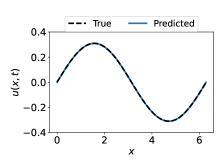
(b) VarianceNO

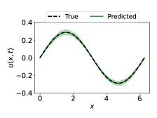
(c) MC-DropoutNO

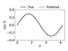
(d) EnsembleNO

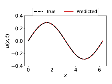
(e) DiverseNO

Figure 19: 1-d Heat equation, in-domain, $k^{\text{train}},k^{\text{test}}\in[1,5]$. Uncertainty estimates from different UQ methods for in-domain values of the input diffusivity coefficient $k$.

Figures 19-22 show the solution profiles for the “easy” smooth and parabolic heat equation with zero Dirichlet boundary conditions for in-domain, small, medium and large OOD shifts, respectively, of the diffusivity parameter $k$. We see that on this “easy” case, most methods are very accurate in-domain in Figure 19 and perform well in the small shift cases in Figure 20. Errors in the BayesianNO, VarianceNO and MC-DropoutNO baselines start to form for medium shifts in Figure 21 and grow in the large shift case in Figure 22. We see both EnsembleNO and DiverseNO output good uncertainty estimates (3 standard deviations) that contain the true solution within these error bounds. See corresponding metric results in Table 3.

Table 3: 1-d heat equation. MSE $\downarrow$, NLL $\downarrow$, n-MeRCI $\downarrow$, RMSCE $\downarrow$ and CRPS $\downarrow$ (mean and standard deviation over 5 seeds) metrics for different UQ methods on the 1-d heat equation in-domain and with small, medium and large OOD shifts, where $k^{\text{train}}\in[1,5]$. Bold indicates values within one standard deviation of the best mean.

	In-domain, $k^{\text{test}}\in[1,5]$
	MSE $\downarrow$	NLL $\downarrow$	n-MeRCI $\downarrow$	RMSCE $\downarrow$	CRPS $\downarrow$
BayesianNO	1.5e-07 (4.9e-08)	-1.3e+04 (2.1e+02)	0.13 ( 0.07)	0.19 ( 0.01)	2.2e-04 (2.8e-05)
VarianceNO	4.1e-07 (2.8e-07)	-1.2e+04 (5.1e+02)	0.18 ( 0.10)	0.15 ( 0.02)	3.1e-04 (9.4e-05)
MC-DropoutNO	3.6e-06 (3.0e-07)	-8.9e+03 (1.8e+02)	0.16 ( 0.07)	0.20 ( 0.00)	1.9e-03 (1.1e-04)
EnsembleNO	1.8e-07 (6.3e-08)	-1.4e+04 (7.5e+02)	0.05 ( 0.02)	0.13 ( 0.01)	1.4e-04 (2.4e-05)
DiverseNO	1.1e-07 (4.3e-08)	-1.5e+04 (7.0e+01)	0.06 ( 0.02)	0.13 ( 0.00)	1.2e-04 (3.5e-06)

	Small OOD shift, $k^{\text{test}}\in[5,6]$
	MSE $\downarrow$	NLL $\downarrow$	n-MeRCI $\downarrow$	RMSCE $\downarrow$	CRPS $\downarrow$
BayesianNO	2.5e-06 (8.6e-07)	-8.5e+03 (1.4e+03)	0.86 ( 0.05)	0.38 ( 0.02)	8.9e-04 (1.9e-04)
VarianceNO	7.1e-06 (3.2e-06)	3.0e+04 (1.2e+04)	1.17 ( 0.11)	0.43 ( 0.02)	1.6e-03 (4.2e-04)
MC-DropoutNO	5.1e-06 (1.4e-06)	-9.4e+03 (2.1e+02)	0.90 ( 0.04)	0.25 ( 0.01)	1.5e-03 (1.0e-04)
EnsembleNO	2.3e-06 (4.9e-07)	-1.1e+04 (7.8e+02)	0.02 ( 0.02)	0.37 ( 0.02)	7.4e-04 (1.2e-04)
DiverseNO	1.7e-06 (4.1e-07)	-1.1e+04 (1.1e+02)	0.05 ( 0.03)	0.35 ( 0.01)	7.3e-04 (5.4e-05)

	Medium OOD shift, $k^{\text{test}}\in[6,7]$
	MSE $\downarrow$	NLL $\downarrow$	n-MeRCI $\downarrow$	RMSCE $\downarrow$	CRPS $\downarrow$
BayesianNO	2.7e-05 (7.5e-06)	2.9e+04 (1.0e+04)	0.84 ( 0.05)	0.47 ( 0.01)	3.4e-03 (6.4e-04)
VarianceNO	8.0e-05 (2.9e-05)	9.0e+05 (2.2e+05)	1.40 ( 0.15)	0.49 ( 0.01)	5.8e-03 (1.4e-03)
MC-DropoutNO	3.9e-05 (1.7e-05)	-7.5e+03 (2.6e+02)	0.90 ( 0.03)	0.37 ( 0.01)	3.4e-03 (6.0e-04)
EnsembleNO	2.4e-05 (3.8e-06)	-8.1e+03 (9.0e+02)	0.03 ( 0.01)	0.38 ( 0.02)	2.5e-03 (3.1e-04)
DiverseNO	1.9e-05 (3.4e-06)	-8.0e+03 (1.0e+02)	0.02 ( 0.00)	0.36 ( 0.01)	2.6e-03 (1.1e-04)

	Large OOD shift, $k^{\text{test}}\in[7,8]$
	MSE $\downarrow$	NLL $\downarrow$	n-MeRCI $\downarrow$	RMSCE $\downarrow$	CRPS $\downarrow$
BayesianNO	1.2e-04 (3.5e-05)	1.5e+05 (3.2e+04)	0.80 ( 0.06)	0.49 ( 0.01)	7.5e-03 (1.5e-03)
VarianceNO	3.7e-04 (1.3e-04)	9.0e+06 (3.0e+06)	1.70 ( 0.20)	0.50 ( 0.00)	1.3e-02 (2.9e-03)
MC-DropoutNO	1.7e-04 (8.0e-05)	-3.0e+03 (1.2e+03)	0.86 ( 0.04)	0.44 ( 0.01)	7.6e-03 (1.7e-03)
EnsembleNO	1.1e-04 (1.6e-05)	-6.6e+03 (9.2e+02)	0.03 ( 0.02)	0.37 ( 0.02)	5.3e-03 (5.9e-04)
DiverseNO	8.8e-05 (1.0e-05)	-6.3e+03 (1.7e+02)	0.03 ( 0.03)	0.36 ( 0.02)	5.8e-03 (8.7e-05)

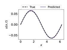
(a) BayesianNO

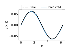
(b) VarianceNO

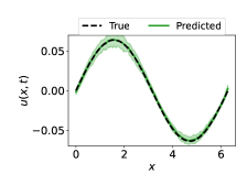
(c) MC-DropoutNO

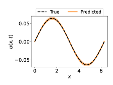
(d) EnsembleNO

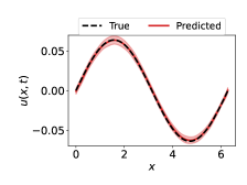
(e) DiverseNO

Figure 20: 1-d Heat equation, small OOD shift, $k^{\text{train}}\in[1,5],k^{\text{test}}\in[5,6]$. Uncertainty estimates from different UQ methods under small OOD shifts in the input diffusivity coefficient $k$.

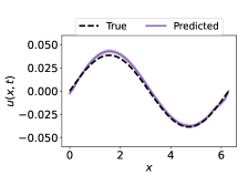
(a) BayesianNO

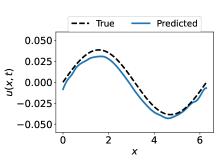
(b) VarianceNO

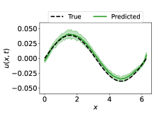
(c) MC-DropoutNO

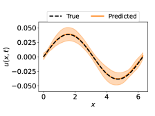
(d) EnsembleNO

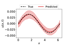
(e) DiverseNO

Figure 21: 1-d Heat equation, medium OOD shift, $k^{\text{train}}\in[1,5],k^{\text{test}}\in[6,7]$. Uncertainty estimates from different UQ methods under medium OOD shifts in the input diffusivity coefficient $k$.

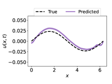
(a) BayesianNO

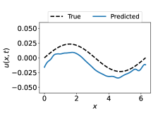
(b) VarianceNO

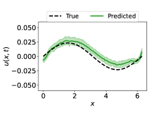
(c) MC-DropoutNO

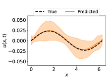
(d) EnsembleNO

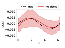
(e) DiverseNO

Figure 22: 1-d Heat equation, large OOD shift, $k^{\text{train}}\in[1,5],k^{\text{test}}\in[7,8]$. Uncertainty estimates from different UQ methods under large OOD shifts in the input diffusivity coefficient $k$.

F.1.2 “Medium” PME

Figures 23-26 show the solution profiles for the “medium” degenerate parabolic PME on an in-domain task and for small, medium and large OOD shifts, respectively, of the power $m$ in the monomial coefficient $k(u)=u^{m}$. The solution for larger values of $m\geq 1$ becomes sharper and more challenging. Figure 23 shows that all methods perform well on the in-domain task with the exception of VarianceNO and MC-DropoutNO having small negative oscillations at the sharp corner (degeneracy point), which separates the region with fluid to the left from the region without fluid to the right. Figure 24 shows the solutions on performing inference on an easier task where the values of $m$ are smaller than those trained on and the corresponding solution is smoother. We see in this easier case that all the methods perform reasonably well. There is left boundary error with the growing in time left boundary condition with VarianceNO, which grows as the OOD shift increases from medium in Figure 25 to large in Figure 26. The medium and large shift cases are particularly more challenging since we train on smaller values of $m$ and perform inference on the sharper cases with increased values $m$. As expected as the problems becomes harder and more challenging for larger $m$ (larger shifts), the uncertainty widens for EnsembleNO and DiverseNO. See corresponding metric results in Table 4.

Table 4: 1-d PME. MSE $\downarrow$, NLL $\downarrow$, n-MeRCI $\downarrow$, RMSCE $\downarrow$ and CRPS $\downarrow$ (mean and standard deviation over 5 seeds) metrics for different UQ methods on the 1-d PME in-domain and with small, medium and large OOD shifts, where $m^{\text{train}}\in[2,3]$. Bold indicates values within one standard deviation of the best mean.

	In-domain, $m^{\text{test}}\in[2,3]$
	MSE $\downarrow$	NLL $\downarrow$	n-MeRCI $\downarrow$	RMSCE $\downarrow$	CRPS $\downarrow$
BayesianNO	7.3e-07 (8.5e-08)	-1.1e+04 (9.8e+01)	0.62 ( 0.08)	0.21 ( 0.00)	5.6e-04 (3.1e-05)
VarianceNO	8.3e-05 (1.8e-05)	-9.4e+03 (7.6e+02)	0.55 ( 0.07)	0.16 ( 0.01)	2.4e-03 (5.9e-04)
MC-DropoutNO	3.2e-05 (1.2e-05)	-6.7e+03 (7.5e+02)	0.40 ( 0.05)	0.22 ( 0.00)	4.2e-03 (2.4e-04)
EnsembleNO	5.3e-07 (1.8e-07)	-1.3e+04 (4.7e+02)	0.18 ( 0.10)	0.18 ( 0.01)	3.4e-04 (7.4e-05)
DiverseNO	1.8e-06 (2.1e-07)	-1.1e+04 (3.3e+02)	0.21 ( 0.06)	0.20 ( 0.01)	6.0e-04 (5.3e-05)

	Small OOD shift, $m^{\text{test}}\in[1,2]$
	MSE $\downarrow$	NLL $\downarrow$	n-MeRCI $\downarrow$	RMSCE $\downarrow$	CRPS $\downarrow$
BayesianNO	1.1e-03 (4.0e-04)	7.7e+05 (2.2e+05)	1.12 ( 0.07)	0.44 ( 0.02)	1.9e-02 (3.5e-03)
VarianceNO	4.0e-03 (2.4e-03)	2.6e+04 (8.8e+03)	0.26 ( 0.06)	0.43 ( 0.03)	3.6e-02 (1.2e-02)
MC-DropoutNO	2.1e-03 (6.0e-04)	1.6e+04 (8.6e+03)	1.18 ( 0.09)	0.36 ( 0.03)	2.5e-02 (4.3e-03)
EnsembleNO	1.2e-03 (2.5e-04)	1.2e+03 (1.8e+03)	0.14 ( 0.03)	0.46 ( 0.01)	1.8e-02 (2.7e-03)
DiverseNO	1.1e-03 (3.7e-04)	7.8e+03 (6.7e+03)	0.21 ( 0.04)	0.42 ( 0.03)	1.7e-02 (3.8e-03)

	Medium OOD shift, $m^{\text{test}}\in[4,5]$
	MSE $\downarrow$	NLL $\downarrow$	n-MeRCI $\downarrow$	RMSCE $\downarrow$	CRPS $\downarrow$
BayesianNO	1.0e-03 (3.2e-04)	1.6e+05 (4.1e+04)	0.73 ( 0.03)	0.47 ( 0.01)	2.1e-02 (3.1e-03)
VarianceNO	5.0e-03 (7.6e-04)	2.4e+07 (7.7e+06)	1.23 ( 0.34)	0.50 ( 0.00)	5.1e-02 (5.2e-03)
MC-DropoutNO	1.5e-03 (4.2e-04)	3.7e+03 (2.9e+03)	0.75 ( 0.02)	0.42 ( 0.03)	2.4e-02 (5.2e-03)
EnsembleNO	8.1e-04 (1.6e-04)	-3.1e+03 (1.0e+03)	0.20 ( 0.03)	0.38 ( 0.01)	1.5e-02 (1.5e-03)
DiverseNO	1.1e-03 (3.5e-04)	-1.8e+03 (3.9e+03)	0.15 ( 0.03)	0.38 ( 0.02)	1.8e-02 (3.3e-03)

	Large OOD shift, $m^{\text{test}}\in[5,6]$
	MSE $\downarrow$	NLL $\downarrow$	n-MeRCI $\downarrow$	RMSCE $\downarrow$	CRPS $\downarrow$
BayesianNO	6.1e-03 (1.9e-03)	8.0e+05 (2.1e+05)	0.69 ( 0.02)	0.49 ( 0.01)	5.4e-02 (8.7e-03)
VarianceNO	2.0e-02 (1.8e-03)	6.9e+08 (4.2e+08)	1.52 ( 0.46)	0.50 ( 0.00)	1.0e-01 (5.8e-03)
MC-DropoutNO	6.4e-03 (2.2e-03)	1.8e+04 (8.3e+03)	0.70 ( 0.02)	0.47 ( 0.03)	5.6e-02 (1.4e-02)
EnsembleNO	4.6e-03 (7.1e-04)	4.4e+02 (1.9e+03)	0.22 ( 0.02)	0.42 ( 0.02)	4.0e-02 (3.0e-03)
DiverseNO	5.8e-03 (1.7e-03)	8.2e+02 (4.5e+03)	0.13 ( 0.05)	0.41 ( 0.02)	4.5e-02 (7.5e-03)

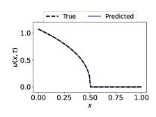
(a) BayesianNO

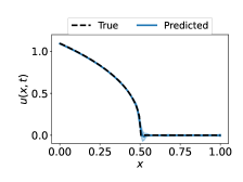
(b) VarianceNO

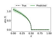
(c) MC-DropoutNO

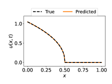
(d) EnsembleNO

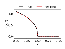
(e) DiverseNO

Figure 23: 1-d PME, in-domain, $m^{\text{train}},m^{\text{test}}\in[2,3]$. Uncertainty estimates from different UQ methods for in-domain values of the power $m$ in the coefficient $k(u)=u^{m}$.

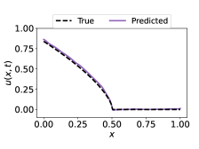
(a) BayesianNO

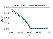
(b) VarianceNO

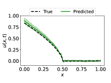
(c) MC-DropoutNO

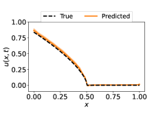
(d) EnsembleNO

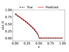
(e) DiverseNO

Figure 24: 1-d PME, small OOD shift, $m^{\text{train}}\in[2,3],m^{\text{test}}\in[1,2]$. Uncertainty estimates from different UQ methods under small OOD shifts in the power $m$ in the coefficient $k(u)=u^{m}$.

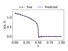
(a) BayesianNO

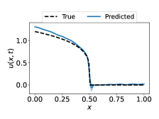
(b) VarianceNO

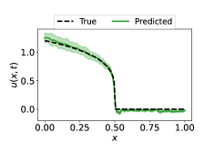
(c) MC-DropoutNO

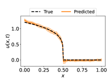
(d) EnsembleNO

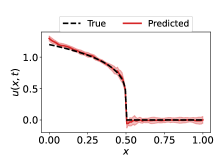
(e) DiverseNO

Figure 25: 1-d PME, medium OOD shift, $m^{\text{train}}\in[2,3],m^{\text{test}}\in[4,5]$. Uncertainty estimates from different UQ methods under medium OOD shifts in the power $m$ in the coefficient $k(u)=u^{m}$.

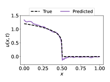
(a) BayesianNO

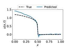
(b) VarianceNO

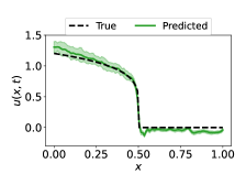
(c) MC-DropoutNO

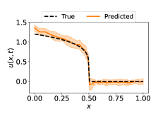
(d) EnsembleNO

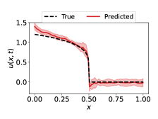
(e) DiverseNO

Figure 26: 1-d PME, large OOD shift, $m^{\text{train}}\in[2,3],m^{\text{test}}\in[5,6]$. Uncertainty estimates from different UQ methods under large OOD shifts in the power $m$ in the coefficient $k(u)=u^{m}$.

F.1.3 “Hard” Stefan Problem

Figures 27-30 show the solution profiles for the “hard” degenerate parabolic, discontinuous GPME, i.e., the Stefan equation, on an in-domain task and for small, medium and large OOD shifts, respectively, of the coefficient $u^{*}$ in $k(u)={\bm{1}}_{u\geq u^{*}}$ in Equation 9, where $u^{*}=u(x^{*}(t),t)$ denotes the solution value at the shock $x^{*}(t)$. The parameter $u^{*}$ also has an effect on the shock position, with smaller values of $u^{*}$ resulting in a faster shock speed. Figure 27 shows that the methods are relatively accurate on the in-domain task with EnsembleNO and DiverseNO exactly capturing the shock with tight uncertainty bounds. The small Gibbs phenomenon at the shock position that occurs with EnsembleNO is damped with DiverseNO. VarianceNO has large uncertainty around the diffused shock. We see that even for small OOD shifts in Figure 28 on this “hard” shock problem, several of the baseline methods suffer numerical artifacts of spurious oscillations, being overly diffusive and having an incorrect shock speed, where the predicted shock position either lags or is ahead of the true shock position, which worsens as the OOD shift increases in Figures 29-30. See corresponding metric results in Table 5.

Table 5: 1-d Stefan equation. MSE $\downarrow$, NLL $\downarrow$, n-MeRCI $\downarrow$, RMSCE $\downarrow$ and CRPS $\downarrow$ (mean and standard deviation over 5 seeds) metrics for different UQ methods on the 1-d Stefan equation in-domain and with small, medium and large OOD shifts, where $u{{}^{*}}^{{\text{train}}}\in[0.6,0.65]$. Bold indicates values within one standard deviation of the best mean.

	In-domain, $u{{}^{*}}^{{\text{test}}}\in[0.6,0.65]$
	MSE $\downarrow$	NLL $\downarrow$	n-MeRCI $\downarrow$	RMSCE $\downarrow$	CRPS $\downarrow$
BayesianNO	3.9e-04 (9.6e-05)	-4.8e+03 (2.6e+02)	0.32 ( 0.11)	0.23 ( 0.00)	9.3e-03 (1.1e-03)
VarianceNO	8.1e-03 (4.7e-04)	-1.1e+04 (5.2e+02)	0.75 ( 0.07)	0.17 ( 0.02)	1.8e-02 (7.4e-04)
MC-DropoutNO	5.8e-04 (1.6e-04)	-2.5e+03 (6.6e+02)	0.33 ( 0.13)	0.17 ( 0.01)	8.1e-03 (1.1e-03)
EnsembleNO	3.6e-04 (2.9e-05)	-7.4e+03 (8.5e+02)	0.41 ( 0.23)	0.12 ( 0.01)	2.7e-03 (1.2e-04)
DiverseNO	3.7e-04 (5.4e-05)	8.7e+03 (5.9e+03)	0.41 ( 0.26)	0.14 ( 0.01)	3.3e-03 (4.8e-04)

	Small OOD shift, $u{{}^{*}}^{{\text{test}}}\in[0.55,0.6]$
	MSE $\downarrow$	NLL $\downarrow$	n-MeRCI $\downarrow$	RMSCE $\downarrow$	CRPS $\downarrow$
BayesianNO	2.0e-02 (1.9e-02)	1.5e+03 (1.3e+03)	0.67 ( 0.15)	0.28 ( 0.01)	4.2e-02 (1.8e-02)
VarianceNO	2.3e-02 (1.6e-03)	7.0e+06 (3.5e+06)	0.97 ( 0.07)	0.40 ( 0.02)	4.3e-02 (1.7e-03)
MC-DropoutNO	9.6e-03 (3.6e-03)	2.4e+04 (8.7e+03)	0.78 ( 0.08)	0.31 ( 0.01)	4.1e-02 (4.4e-03)
EnsembleNO	8.1e-03 (3.4e-03)	-5.2e+03 (3.3e+02)	0.14 ( 0.09)	0.32 ( 0.01)	2.5e-02 (3.6e-03)
DiverseNO	1.4e-02 (2.3e-03)	1.2e+04 (5.5e+03)	0.14 ( 0.06)	0.38 ( 0.01)	3.7e-02 (3.3e-03)

	Medium OOD shift, $u{{}^{*}}^{{\text{test}}}\in[0.7,0.75]$
	MSE $\downarrow$	NLL $\downarrow$	n-MeRCI $\downarrow$	RMSCE $\downarrow$	CRPS $\downarrow$
BayesianNO	1.7e-02 (1.4e-02)	6.0e+03 (3.6e+03)	0.66 ( 0.10)	0.29 ( 0.02)	4.6e-02 (7.6e-03)
VarianceNO	3.2e-02 (1.3e-03)	1.9e+07 (8.4e+06)	0.83 ( 0.05)	0.40 ( 0.02)	5.2e-02 (1.4e-03)
MC-DropoutNO	2.9e-02 (1.3e-02)	2.2e+04 (9.8e+03)	0.56 ( 0.26)	0.36 ( 0.03)	6.4e-02 (1.0e-02)
EnsembleNO	8.0e-03 (1.4e-03)	-4.3e+03 (1.5e+02)	0.07 ( 0.03)	0.33 ( 0.02)	3.3e-02 (3.3e-03)
DiverseNO	1.1e-02 (3.6e-03)	2.0e+04 (3.8e+03)	0.14 ( 0.03)	0.37 ( 0.04)	4.1e-02 (6.8e-03)

	Large OOD shift, $u{{}^{*}}^{{\text{test}}}\in[0.5,0.55]$
	MSE $\downarrow$	NLL $\downarrow$	n-MeRCI $\downarrow$	RMSCE $\downarrow$	CRPS $\downarrow$
BayesianNO	1.7e-01 (1.7e-01)	1.9e+04 (5.3e+03)	0.50 ( 0.25)	0.40 ( 0.03)	1.5e-01 (7.2e-02)
VarianceNO	3.4e-02 (1.8e-03)	2.7e+07 (1.4e+07)	0.99 ( 0.09)	0.45 ( 0.01)	6.6e-02 (1.7e-03)
MC-DropoutNO	4.4e-02 (3.1e-02)	7.3e+04 (1.2e+04)	0.54 ( 0.11)	0.42 ( 0.01)	1.1e-01 (1.5e-02)
EnsembleNO	4.6e-02 (1.9e-02)	-2.2e+03 (3.9e+02)	0.37 ( 0.14)	0.36 ( 0.01)	8.2e-02 (1.0e-02)
DiverseNO	8.9e-02 (5.1e-02)	2.1e+04 (6.8e+03)	0.24 ( 0.11)	0.43 ( 0.01)	1.3e-01 (2.9e-02)

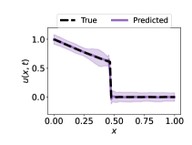
(a) BayesianNO

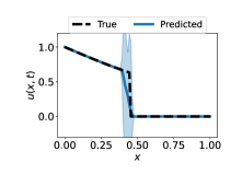
(b) VarianceNO

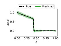
(c) MC-DropoutNO

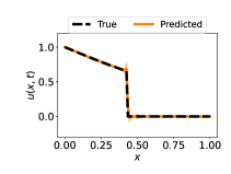
(d) EnsembleNO

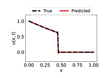
(e) DiverseNO

Figure 27: 1-d Stefan Equation, in-domain, $u{{}^{*}}^{{\text{train}}},u{{}^{*}}^{{\text{test}}}\in[0.6,0.65]$. Uncertainty estimates from different UQ methods for in-domain values for the solution value at the shock $u(t,x^{*}(t))=u^{*}$ for shock position $x^{*}(t)$.

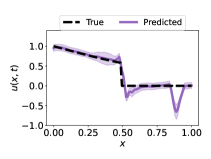
(a) BayesianNO

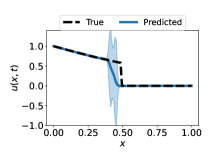
(b) VarianceNO

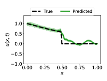
(c) MC-DropoutNO

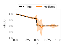
(d) EnsembleNO

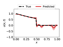
(e) DiverseNO

Figure 28: 1-d Stefan Equation, small OOD shift, $u{{}^{*}}^{{\text{train}}}\in[0.6,0.65],u{{}^{*}}^{{\text{test}}}\in[0.55,0.6]$. Uncertainty estimates from different UQ methods under small OOD shifts in the solution value at the shock $u(t,x^{*}(t))=u^{*}$ for shock position $x^{*}(t)$.

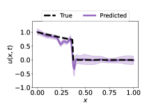
(a) BayesianNO

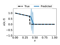
(b) VarianceNO

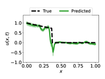
(c) MC-DropoutNO

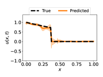
(d) EnsembleNO

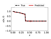
(e) DiverseNO

Figure 29: 1-d Stefan Equation, medium OOD shift, $u{{}^{*}}^{{\text{train}}}\in[0.6,0.65],u{{}^{*}}^{{\text{test}}}\in[0.7,0.75]$. Uncertainty estimates from different UQ methods under medium OOD shifts in the solution value at the shock $u(x^{*}(t),t)=u^{*}$ for shock position $x^{*}(t)$.

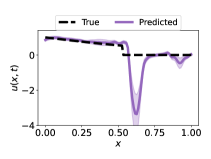
(a) BayesianNO

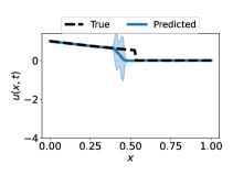
(b) VarianceNO

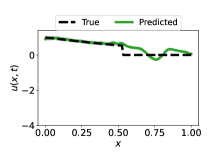
(c) MC-DropoutNO

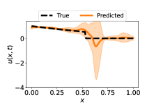
(d) EnsembleNO

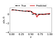
(e) DiverseNO

Figure 30: 1-d Stefan Equation, large OOD shift, $u{{}^{*}}^{{\text{train}}}\in[0.6,0.65],u{{}^{*}}^{{\text{test}}}\in[0.5,0.55]$. Uncertainty estimates from different UQ methods under large OOD shifts in the solution value at the shock $u(x^{*}(t),t)=u^{*}$ for shock position $x^{*}(t)$.

F.1.4 Hyperbolic Linear Advection Equation

Figures 31-34 show the solution profiles for the hyperbolic linear advection equation conditions for an in-domain task, and for small, medium and large OOD shifts, respectively, of the velocity parameter $\beta>0$. The solution is a rightward moving shock, where $\beta$ controls the shock speed. We see that in this difficult shock case the baseline methods, e.g., BayesianNO, VarianceNO and MC-DropoutNO suffer from numerical artifacts of artificial oscillations, being over-diffusive and lagging of the shock position. Only EnsembleNO and our DiverseNO accurately capture the shock location and have the largest uncertainty there. See corresponding metric results in Table 6.

Table 6: 1-d Linear Advection MSE $\downarrow$, NLL $\downarrow$, n-MeRCI $\downarrow$, RMSCE $\downarrow$ and CRPS $\downarrow$ (mean and standard deviation over 5 seeds) metrics for different UQ methods on the 1-d linear advection equation in-domain and with small, medium and large OOD shifts, where $\beta^{\text{train}}\in[1,2]$. Bold indicates values within one standard deviation of the best mean.

	In-domain, $\beta^{\text{test}}\in[1,2]$
	MSE $\downarrow$	NLL $\downarrow$	n-MeRCI $\downarrow$	RMSCE $\downarrow$	CRPS $\downarrow$
BayesianNO	2.0e-04 (3.6e-05)	-5.7e+03 (1.6e+02)	0.59 ( 0.08)	0.23 ( 0.00)	6.2e-03 (6.2e-04)
VarianceNO	2.2e-02 (3.4e-02)	-1.1e+04 (2.6e+03)	0.41 ( 0.18)	0.20 ( 0.03)	1.8e-02 (1.6e-02)
MC-DropoutNO	2.8e-04 (5.0e-05)	-5.0e+03 (2.3e+02)	0.67 ( 0.15)	0.20 ( 0.00)	7.7e-03 (5.1e-04)
EnsembleNO	2.0e-04 (1.1e-05)	-1.1e+04 (1.8e+02)	0.40 ( 0.06)	0.12 ( 0.00)	1.2e-03 (5.8e-05)
DiverseNO	2.0e-04 (2.6e-05)	-7.2e+03 (9.6e+02)	0.28 ( 0.08)	0.12 ( 0.01)	1.7e-03 (1.1e-04)

	Out-of-domain, $\beta^{\text{test}}\in[0.5,1]$
	MSE $\downarrow$	NLL $\downarrow$	n-MeRCI $\downarrow$	RMSCE $\downarrow$	CRPS $\downarrow$
BayesianNO	6.8e-02 (1.6e-02)	1.7e+05 (9.3e+04)	0.77 ( 0.05)	0.27 ( 0.03)	1.1e-01 (2.7e-02)
VarianceNO	7.3e-02 (2.8e-02)	9.4e+07 (6.0e+07)	0.46 ( 0.20)	0.40 ( 0.03)	7.9e-02 (1.2e-02)
MC-DropoutNO	3.0e-02 (9.1e-03)	5.9e+04 (2.3e+04)	0.93 ( 0.03)	0.26 ( 0.03)	7.3e-02 (1.8e-02)
EnsembleNO	3.0e-02 (3.8e-03)	-3.5e+03 (3.6e+02)	0.17 ( 0.03)	0.28 ( 0.02)	6.0e-02 (5.1e-03)
DiverseNO	4.3e-02 (3.4e-02)	4.6e+04 (3.2e+04)	0.16 ( 0.06)	0.35 ( 0.03)	7.1e-02 (3.2e-02)

	Out-of-domain, $\beta^{\text{test}}\in[2.5,3]$
	MSE $\downarrow$	NLL $\downarrow$	n-MeRCI $\downarrow$	RMSCE $\downarrow$	CRPS $\downarrow$
BayesianNO	6.4e-03 (1.7e-03)	4.6e+03 (3.7e+03)	0.76 ( 0.05)	0.41 ( 0.02)	3.7e-02 (4.1e-03)
VarianceNO	4.4e-02 (4.0e-02)	1.4e+07 (1.7e+07)	0.42 ( 0.30)	0.45 ( 0.03)	3.9e-02 (1.6e-02)
MC-DropoutNO	3.8e-03 (6.8e-04)	2.9e+03 (2.9e+03)	0.80 ( 0.05)	0.30 ( 0.01)	2.3e-02 (1.6e-03)
EnsembleNO	4.3e-03 (4.2e-04)	-2.3e+03 (7.7e+02)	0.45 ( 0.04)	0.44 ( 0.01)	3.1e-02 (2.7e-03)
DiverseNO	7.4e-03 (2.5e-03)	1.1e+04 (1.0e+04)	0.25 ( 0.15)	0.45 ( 0.03)	4.1e-02 (2.8e-03)

	Out-of-domain, $\beta^{\text{test}}\in[3,3.5]$
	MSE $\downarrow$	NLL $\downarrow$	n-MeRCI $\downarrow$	RMSCE $\downarrow$	CRPS $\downarrow$
BayesianNO	1.5e-02 (3.4e-03)	1.5e+04 (6.7e+03)	0.71 ( 0.06)	0.46 ( 0.01)	7.4e-02 (8.5e-03)
VarianceNO	5.3e-02 (4.2e-02)	1.8e+08 (3.0e+08)	0.38 ( 0.26)	0.47 ( 0.02)	5.1e-02 (1.6e-02)
MC-DropoutNO	7.4e-03 (1.2e-03)	7.8e+03 (3.6e+03)	0.75 ( 0.04)	0.37 ( 0.02)	3.7e-02 (1.8e-03)
EnsembleNO	1.0e-02 (1.3e-03)	1.0e+03 (1.0e+03)	0.42 ( 0.10)	0.47 ( 0.00)	6.3e-02 (4.7e-03)
DiverseNO	1.8e-02 (3.7e-03)	2.1e+04 (1.8e+04)	0.27 ( 0.17)	0.47 ( 0.03)	8.1e-02 (7.0e-03)

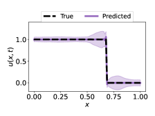
(a) BayesianNO

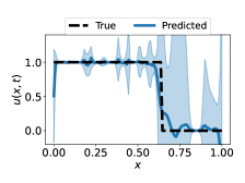
(b) VarianceNO

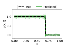
(c) MC-DropoutNO

(d) EnsembleNO

(e) DiverseNO

Figure 31: 1-d Linear advection, in-domain, $\beta^{\text{train}},\beta^{\text{test}}\in[1,2]$. Uncertainty estimates from different UQ methods for in-domain values of the input velocity $\beta$ coefficient.

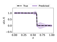
(a) BayesianNO

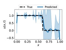
(b) VarianceNO

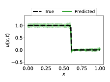
(c) MC-DropoutNO

(d) EnsembleNO

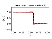
(e) DiverseNO

Figure 32: 1-d Linear advection, small OOD shift, $\beta^{\text{train}}\in[1,2],\beta^{\text{test}}\in[0.5,1]$. Uncertainty estimates from different UQ methods under small OOD shifts in the input velocity $\beta$ coefficient.

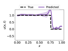
(a) BayesianNO

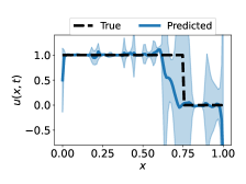
(b) VarianceNO

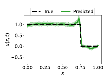
(c) MC-DropoutNO

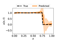
(d) EnsembleNO

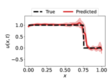
(e) DiverseNO

Figure 33: 1-d Linear advection, medium OOD shift, $\beta^{\text{train}}\in[1,2],\beta^{\text{test}}\in[2.5,3]$. Uncertainty estimates from different UQ methods under medium OOD shifts in the input velocity $\beta$ coefficient.

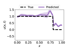
(a) BayesianNO

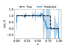
(b) VarianceNO

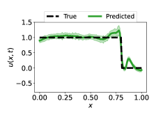
(c) MC-DropoutNO

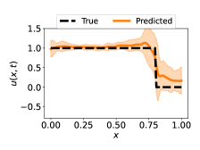
(d) EnsembleNO

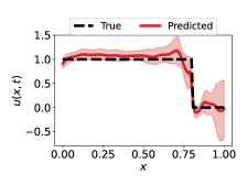
(e) DiverseNO

Figure 34: 1-d Linear advection, large OOD shift, $\beta^{\text{train}}\in[1,2],\beta^{\text{test}}\in[3,3.5]$. Uncertainty estimates from different UQ methods under large OOD shifts in the input velocity $\beta$ coefficient.

F.2 Cost performance curves

Here we show the the cost performance curves as a function of the number parameters. We see in Figure 35 that it has similar trends to the cost performance curves as a function of the floating point operations (FLOPS) in Figure 5. DiverseNO has lower MSE and n-MeRCI values for the same number of parameters as EnsembleNO and hence is more computationally efficient on both the heat equation and PME.

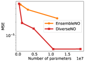
(a) Heat, MSE $\downarrow$

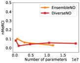
(b) Heat, n-MeRCI $\downarrow$

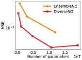
(c) PME, MSE $\downarrow$

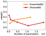
(d) PME, n-MeRCI $\downarrow$

Figure 35: Cost-performance tradeoff. MSE $\downarrow$ and n-MeRCI $\downarrow$ vs number of parameters for EnsembleNO and DiverseNO with varying number of parameters. for (a-b) 1-d Heat equation, medium OOD shift, i.e., $k^{\text{train}}\in[1,5],k^{\text{test}}\in[6,7]$ and (c-d) 1-d PME, medium OOD shift, i.e., $m^{\text{train}}\in[2,3],m^{\text{test}}\in[4,5]$.

F.3 Effect of ProbConserv update

Table 7: Effect of ProbConserv update, 1-d heat equation. MSE $\downarrow$, Conservation Error (CE) (should be zero) and n-MeRCI $\downarrow$ (mean and standard deviation over 5 seeds) for different UQ methods with and without ProbConserv evaluated on 1-d heat equation with small, medium and large OOD shifts, where $k^{\text{train}}\in[1,5]$. Bold indicates values within one standard deviation of the best mean.

	Small OOD shift, $k^{\text{test}}\in[5,6]$
	MSE $\downarrow$		CE (should be zero)		n-MeRCI $\downarrow$
	Standard	+ ProbConserv	Standard	+ ProbConserv	Standard	+ ProbConserv
BayesianNO	2.5e-06 (8.6e-07)	2.3e-06 (8.5e-07)	0.01 ( 0.00)	0.00 ( 0.00)	0.86 ( 0.05)	0.86 ( 0.05)
VarianceNO	7.1e-06 (3.2e-06)	5.5e-06 (1.2e-06)	0.01 ( 0.01)	0.00 ( 0.00)	1.17 ( 0.11)	1.17 ( 0.12)
MC-DropoutNO	5.1e-06 (1.4e-06)	4.9e-06 (1.5e-06)	0.01 ( 0.00)	0.00 ( 0.00)	0.90 ( 0.04)	0.91 ( 0.05)
EnsembleNO	2.3e-06 (4.9e-07)	2.2e-06 (5.2e-07)	0.00 ( 0.00)	0.00 ( 0.00)	0.02 ( 0.02)	0.02 ( 0.01)
DiverseNO	1.7e-06 (4.1e-07)	1.2e-06 (9.2e-07)	0.01 ( 0.01)	0.00 ( 0.00)	0.05 ( 0.03)	0.05 ( 0.03)

	Medium OOD shift, $k^{\text{test}}\in[6,7]$
	MSE $\downarrow$		CE (should be zero)		n-MeRCI $\downarrow$
	Standard	+ ProbConserv	Standard	+ ProbConserv	Standard	+ ProbConserv
BayesianNO	2.7e-05 (7.5e-06)	2.6e-05 (7.7e-06)	0.02 ( 0.01)	0.00 ( 0.00)	0.84 ( 0.05)	0.84 ( 0.05)
VarianceNO	8.0e-05 (2.9e-05)	6.7e-05 (1.3e-05)	0.04 ( 0.03)	0.00 ( 0.00)	1.40 ( 0.15)	1.41 ( 0.16)
MC-DropoutNO	3.9e-05 (1.7e-05)	3.7e-05 (1.8e-05)	0.03 ( 0.01)	0.00 ( 0.00)	0.90 ( 0.03)	0.90 ( 0.04)
EnsembleNO	2.4e-05 (3.8e-06)	2.4e-05 (4.1e-06)	0.01 ( 0.00)	0.00 ( 0.00)	0.03 ( 0.01)	0.03 ( 0.02)
DiverseNO	1.9e-05 (3.4e-06)	1.3e-05 (1.1e-05)	0.05 ( 0.03)	0.00 ( 0.00)	0.02 ( 0.00)	0.08 ( 0.08)

	Large OOD shift, $k^{\text{test}}\in[7,8]$
	MSE $\downarrow$		CE (should be zero)		n-MeRCI $\downarrow$
	Standard	+ ProbConserv	Standard	+ ProbConserv	Standard	+ ProbConserv
BayesianNO	1.2e-04 (3.5e-05)	1.2e-04 (3.6e-05)	0.04 ( 0.02)	0.00 ( 0.00)	0.80 ( 0.06)	0.80 ( 0.06)
VarianceNO	3.7e-04 (1.3e-04)	3.2e-04 (7.3e-05)	0.08 ( 0.07)	0.01 ( 0.01)	1.70 ( 0.20)	1.69 ( 0.21)
MC-DropoutNO	1.7e-04 (8.0e-05)	1.6e-04 (8.3e-05)	0.06 ( 0.02)	0.00 ( 0.00)	0.86 ( 0.04)	0.86 ( 0.04)
EnsembleNO	1.1e-04 (1.6e-05)	1.1e-04 (1.6e-05)	0.01 ( 0.00)	0.00 ( 0.00)	0.03 ( 0.02)	0.03 ( 0.01)
DiverseNO	8.8e-05 (1.0e-05)	5.8e-05 (5.1e-05)	0.10 ( 0.06)	0.00 ( 0.00)	0.03 ( 0.03)	0.12 ( 0.11)

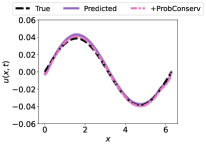
(a) BayesianNO

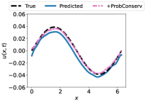
(b) VarianceNO

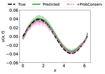
(c) MC-DropoutNO

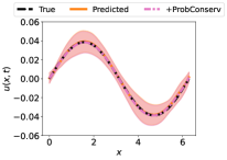
(d) EnsembleNO

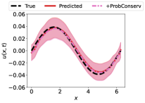
(e) DiverseNO

Figure 36: 1-d Heat equation, medium OOD shift, $k^{\text{train}}\in[1,5],k^{\text{test}}\in[6,7]$. Uncertainty estimates from different UQ methods under medium OOD shifts in the input diffusivity coefficient with adding ProbConserv onto the uncertainty estimates. ProbConserv improves the OOD predictions for all UQ estimates on this “easy” task.

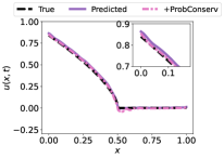
(a) BayesianNO

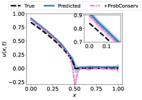
(b) VarianceNO

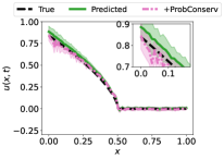
(c) MC-DropoutNO

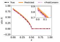
(d) EnsembleNO

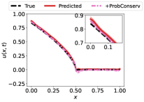
(e) DiverseNO

Figure 37: 1-d PME equation, small OOD shift, $m^{\text{train}}\in[2,3],m^{\text{test}}\in[1,2]$. Uncertainty estimates from different UQ methods under small OOD shifts in the power $m$ in the coefficient $k(u)=u^{m}$ with adding ProbConserv onto the uncertainty estimates. ProbConserv improves the OOD predictions for all methods except for VarianceNO whose UQ estimate is not well-correlated with the error.

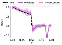
(a) BayesianNO

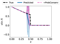
(b) VarianceNO

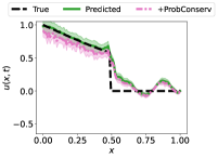
(c) MC-DropoutNO

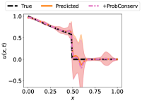
(d) EnsembleNO

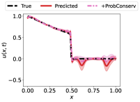
(e) DiverseNO

Figure 38: 1-d Stefan Equation, small OOD shift, $u{{}^{*}}^{{\text{train}}}\in[0.6,0.65],u{{}^{*}}^{{\text{test}}}\in[0.55,0.6]$. Solution profiles after applying ProbConserv over different UQ methods under small OOD shifts in the solution value at the shock $u(t,x^{*}(t))=u^{*}$ for shock position $x^{*}(t)$. ProbConserv improves the OOD prediction with DiverseNO whose UQ estimate is well-correlated with the error and damps the artificial oscillations.

Table 8: Effect of ProbConserv update, 1-d PME. MSE $\downarrow$, Conservation Error (CE) (should be zero) and n-MeRCI $\downarrow$ (mean and standard deviation over 5 seeds) for different UQ methods with and without ProbConserv evaluated on 1-d PME with small, medium and large OOD shifts, where $m^{\text{train}}\in[2,3]$. Bold indicates values within one standard deviation of the best mean.

	Small OOD shift, $m^{\text{test}}\in[1,2]$
	MSE $\downarrow$		CE (should be zero)		n-MeRCI $\downarrow$
	Standard	+ ProbConserv	Standard	+ ProbConserv	Standard	+ ProbConserv
BayesianNO	1.1e-03 (4.0e-04)	3.8e-04 (1.4e-04)	0.38 ( 0.07)	0.02 ( 0.00)	1.12 ( 0.07)	1.13 ( 0.07)
VarianceNO	4.0e-03 (2.4e-03)	8.6e-03 (4.3e-03)	0.75 ( 0.27)	0.00 ( 0.00)	0.26 ( 0.06)	0.22 ( 0.05)
MC-DropoutNO	2.1e-03 (6.0e-04)	8.6e-04 (2.1e-04)	0.52 ( 0.10)	0.00 ( 0.00)	1.18 ( 0.09)	1.17 ( 0.09)
EnsembleNO	1.2e-03 (2.5e-04)	1.7e-04 (1.1e-04)	0.40 ( 0.06)	0.00 ( 0.00)	0.14 ( 0.03)	0.08 ( 0.06)
DiverseNO	1.1e-03 (3.7e-04)	3.9e-04 (6.6e-05)	0.37 ( 0.09)	0.00 ( 0.00)	0.21 ( 0.04)	0.20 ( 0.04)

	Medium OOD shift, $m^{\text{test}}\in[4,5]$
	MSE $\downarrow$		CE (should be zero)		n-MeRCI $\downarrow$
	Standard	+ ProbConserv	Standard	+ ProbConserv	Standard	+ ProbConserv
BayesianNO	1.0e-03 (3.2e-04)	7.8e-04 (1.9e-04)	0.31 ( 0.08)	0.00 ( 0.00)	0.73 ( 0.03)	0.73 ( 0.03)
VarianceNO	5.0e-03 (7.6e-04)	7.0e-02 (1.0e-02)	0.90 ( 0.14)	0.01 ( 0.01)	1.23 ( 0.34)	1.25 ( 0.31)
MC-DropoutNO	1.5e-03 (4.2e-04)	1.1e-03 (3.6e-04)	0.35 ( 0.12)	0.00 ( 0.00)	0.75 ( 0.02)	0.74 ( 0.02)
EnsembleNO	8.1e-04 (1.6e-04)	5.3e-04 (8.1e-05)	0.27 ( 0.03)	0.00 ( 0.00)	0.20 ( 0.03)	0.14 ( 0.07)
DiverseNO	1.1e-03 (3.5e-04)	9.9e-04 (6.2e-04)	0.32 ( 0.06)	0.00 ( 0.00)	0.15 ( 0.03)	0.09 ( 0.06)

	Large OOD shift, $m^{\text{test}}\in[5,6]$
	MSE $\downarrow$		CE (should be zero)		n-MeRCI $\downarrow$
	Standard	+ ProbConserv	Standard	+ ProbConserv	Standard	+ ProbConserv
BayesianNO	6.1e-03 (1.9e-03)	4.7e-03 (1.3e-03)	0.83 ( 0.19)	0.01 ( 0.00)	0.69 ( 0.02)	0.69 ( 0.02)
VarianceNO	2.0e-02 (1.8e-03)	3.3e-01 (8.5e-02)	1.87 ( 0.18)	0.07 ( 0.06)	1.52 ( 0.46)	1.55 ( 0.45)
MC-DropoutNO	6.4e-03 (2.2e-03)	3.5e-03 (1.4e-03)	0.81 ( 0.24)	0.00 ( 0.00)	0.70 ( 0.02)	0.66 ( 0.03)
EnsembleNO	4.6e-03 (7.1e-04)	2.5e-03 (5.2e-04)	0.71 ( 0.05)	0.00 ( 0.00)	0.22 ( 0.02)	0.15 ( 0.06)
DiverseNO	5.8e-03 (1.7e-03)	4.4e-03 (2.6e-03)	0.82 ( 0.15)	0.00 ( 0.00)	0.13 ( 0.05)	0.06 ( 0.03)

In this section, we report the solution profiles and metrics, which compare the effect of using the various UQ estimates for NOs within the ProbConserv framework. Tables 7-9 show that the conservation error (CE) after applying ProbConserv is 0, and that the CE for the unconstrained models can be quite large, especially on the harder tasks. The results on the “easy” heat equation task in Figure 36 and corresponding Table 7 show that ProbConserv improves the MSE for all the UQ methods. The results on the “harder” problems in Figure 37 and corresponding Table 8 for the PME and Figure 38 and corresponding Table 9 for the Stefan equation show the impact of good uncertainty estimates as input to ProbConserv. We see that ProbConserv improves the solution profiles and MSE for the methods except for VarianceNO, whose UQ estimate is not well-correlated with the error.

Table 9: Effect of ProbConserv update, 1-d Stefan. MSE $\downarrow$, Conservation Error (CE) (should be zero) and n-MeRCI $\downarrow$ (mean and standard deviation over 5 seeds) for different UQ methods with and without ProbConserv evaluated on the 1-d Stefan equation with small, medium and large OOD shifts, where $u{{}^{*}}^{{\text{train}}}\in[0.6,0.65]$. Bold indicates values within one standard deviation of the best mean.

	Small OOD shift, ${u^{*}}^{\text{test}}\in[0.55,0.6]$
	MSE $\downarrow$		CE (should be zero)		n-MeRCI $\downarrow$
	Standard	+ ProbConserv	Standard	+ ProbConserv	Standard	+ ProbConserv
BayesianNO	2.0e-02 (1.9e-02)	1.4e-02 (8.5e-03)	0.37 ( 0.23)	0.00 ( 0.00)	0.67 ( 0.15)	0.66 ( 0.17)
VarianceNO	2.3e-02 (1.6e-03)	3.0e-02 (3.6e-03)	1.08 ( 0.06)	0.00 ( 0.00)	0.97 ( 0.07)	0.95 ( 0.03)
MC-DropoutNO	9.6e-03 (3.6e-03)	9.5e-03 (3.2e-03)	0.51 ( 0.21)	0.00 ( 0.00)	0.78 ( 0.08)	0.77 ( 0.08)
EnsembleNO	8.1e-03 (3.4e-03)	9.1e-03 (2.9e-03)	0.20 ( 0.03)	0.00 ( 0.00)	0.14 ( 0.09)	0.23 ( 0.06)
DiverseNO	1.4e-02 (2.3e-03)	1.1e-02 (9.2e-04)	0.27 ( 0.05)	0.00 ( 0.00)	0.14 ( 0.06)	0.11 ( 0.07)

	Medium OOD shift, ${u^{*}}^{\text{test}}\in[0.7,0.75]$
	MSE $\downarrow$		CE (should be zero)		n-MeRCI $\downarrow$
	Standard	+ ProbConserv	Standard	+ ProbConserv	Standard	+ ProbConserv
BayesianNO	1.7e-02 (1.4e-02)	1.3e-02 (3.8e-03)	0.55 ( 0.19)	0.00 ( 0.00)	0.66 ( 0.10)	0.66 ( 0.10)
VarianceNO	3.2e-02 (1.3e-03)	4.1e-02 (5.3e-03)	1.14 ( 0.05)	0.00 ( 0.00)	0.83 ( 0.05)	0.84 ( 0.04)
MC-DropoutNO	2.9e-02 (1.3e-02)	1.8e-02 (1.1e-02)	1.01 ( 0.32)	0.00 ( 0.00)	0.56 ( 0.26)	0.57 ( 0.25)
EnsembleNO	8.0e-03 (1.4e-03)	7.1e-03 (5.6e-04)	0.52 ( 0.08)	0.00 ( 0.00)	0.07 ( 0.03)	0.24 ( 0.11)
DiverseNO	1.1e-02 (3.6e-03)	9.5e-03 (1.8e-03)	0.59 ( 0.19)	0.00 ( 0.00)	0.14 ( 0.03)	0.12 ( 0.03)

	Large OOD shift, ${u^{*}}^{\text{test}}\in[0.5,0.55]$
	MSE $\downarrow$		CE (should be zero)		n-MeRCI $\downarrow$
	Standard	+ ProbConserv	Standard	+ ProbConserv	Standard	+ ProbConserv
BayesianNO	1.7e-01 (1.7e-01)	7.7e-02 (4.7e-02)	1.34 ( 0.94)	0.00 ( 0.00)	0.50 ( 0.25)	0.48 ( 0.27)
VarianceNO	3.4e-02 (1.8e-03)	7.9e-02 (8.8e-03)	1.72 ( 0.07)	0.00 ( 0.00)	0.99 ( 0.09)	0.97 ( 0.05)
MC-DropoutNO	4.4e-02 (3.1e-02)	4.0e-02 (2.7e-02)	1.27 ( 0.41)	0.00 ( 0.00)	0.54 ( 0.11)	0.44 ( 0.06)
EnsembleNO	4.6e-02 (1.9e-02)	4.7e-02 (1.5e-02)	0.61 ( 0.13)	0.00 ( 0.00)	0.37 ( 0.14)	0.33 ( 0.13)
DiverseNO	8.9e-02 (5.1e-02)	6.4e-02 (2.6e-02)	0.90 ( 0.39)	0.00 ( 0.00)	0.24 ( 0.11)	0.21 ( 0.11)

References

- Alesiani et al. (2022) Francesco Alesiani, Makoto Takamoto, and Mathias Niepert. HyperFNO: Improving the generalization behavior of Fourier Neural Operators. In NeurIPS 2022 Workshop on Machine Learning and Physical Sciences, 2022.
- Benitez et al. (2023) J. Antonio Lara Benitez, Takashi Furuya, Florian Faucher, Anastasis Kratsios, Xavier Tricoche, and Maarten V. de Hoop. Out-of-distributional risk bounds for neural operators with applications to the Helmholtz equation. arXiv preprint arXiv:2301.11509, 2023.
- Boullé & Townsend (2023) Nicolas Boullé and Alex Townsend. A mathematical guide to operator learning. arXiv preprint arXiv:2312.14688, 2023.
- Bourel et al. (2020) Mathias Bourel, Jairo Cugliari, Yannig Goude, and Jean-Michel Poggi. Boosting diversity in regression ensembles. Statistical Analysis and Data Mining: The ASA Data Science Journal, 2020.
- Brunton et al. (2016) Steven L Brunton, Joshua L Proctor, and J Nathan Kutz. Discovering governing equations from data by sparse identification of nonlinear dynamical systems. Proceedings of the National Academy of Sciences, 113(15):3932–3937, 2016.
- Chatterjee & Hadi (1988) S. Chatterjee and A.S. Hadi. Sensitivity Analysis in Linear Regression. John Wiley & Sons, New York, 1988.
- Conti et al. (2023) Paolo Conti, Giorgio Gobat, Stefania Fresca, Andrea Manzoni, and Attilio Frangi. Reduced order modeling of parametrized systems through autoencoders and sindy approach: continuation of periodic solutions. Computer Methods in Applied Mechanics and Engineering, 411:116072, 2023.
- Dandekar et al. (2022) Raj Dandekar, Karen Chung, Vaibhav Dixit, Mohamed Tarek, Aslan Garcia-Valadez, Krishna Vishal Vemula, and Chris Rackauckas. Bayesian Neural Ordinary Differential Equations. arXiv preprint arXiv:2012.07244, 2022.
- de Hoop et al. (2022) Maarten V. de Hoop, Daniel Zhengyu Huang, Elizabeth Qian, and Andrew M. Stuart. The Cost-Accuracy Trade-Off In Operator Learning With Neural Networks, August 2022.
- Edwards (2022) Chris Edwards. Neural networks learn to speed up simulations. Communications of the ACM, 65(5):27–29, 2022.
- Gal & Ghahramani (2016) Yarin Gal and Zoubin Ghahramani. Dropout as a bayesian approximation: Representing model uncertainty in deep learning. In International Conference on Machine Learning, pp. 1050–1059. PMLR, 2016.
- Gneiting & Raftery (2007) Tilmann Gneiting and Adrian E. Raftery. Strictly proper scoring rules, prediction, and estimation. Journal of the American Statistical Association, 102(477):359 – 378, 2007.
- Gneiting et al. (2007) Tilmann Gneiting, Fadoua Balabdaoui, and Adrian E Raftery. Probabilistic forecasts, calibration and sharpness. Journal of the Royal Statistical Society Series B: Statistical Methodology, 69(2):243–268, 2007.
- Graves (2011) Alex Graves. Practical variational inference for neural networks. In Advances in Neural Information Processing Systems, volume 24, 2011.
- Gupta et al. (2021) Gaurav Gupta, Xiongye Xiao, and Paul Bogdan. Multiwavelet-based operator learning for differential equations. In Advances in Neural Information Processing Systems, volume 34, pp. 24048–24062, 2021.
- Hansen et al. (2023) Derek Hansen, Danielle C. Maddix, Shima Alizadeh, Gaurav Gupta, and Michael W Mahoney. Learning physical models that can respect conservation laws. In International Conference on Machine Learning, volume 202, pp. 12469–12510. PMLR, 2023.
- Hodgkinson et al. (2022) Liam Hodgkinson, Chris van der Heide, Fred Roosta, and Michael W. Mahoney. Monotonicity and Double Descent in Uncertainty Estimation with Gaussian Processes. arXiv preprint arXiv:2210.07612, 2022.
- Hodgkinson et al. (2023) Liam Hodgkinson, Chris van der Heide, Robert Salomone, Fred Roosta, and Michael W. Mahoney. The interpolating information criterion for overparameterized models. arXiv preprint arXiv:2307.07785, 2023.
- Hughes (2000) Thomas J.R. Hughes. The Finite Element Method: Linear Static and Dynamic Finite Element Analysis. Dover Publications, 2000.
- Kim et al. (2019) Hyunjik Kim, Andriy Mnih, Jonathan Schwarz, Marta Garnelo, Ali Eslami, Dan Rosenbaum, Oriol Vinyals, and Yee Whye Teh. Attentive Neural Processes. arXiv preprint arXiv:1901.05761, 2019.
- Kovachki et al. (2021) Nikola Kovachki, Zongyi Li, Burigede Liu, Kamyar Azizzadenesheli, Kaushik Bhattacharya, Andrew Stuart, and Anima Anandkumar. Neural operator: Learning maps between function spaces. arXiv preprint arXiv:2108.08481, 2021.
- Krishnapriyan et al. (2021) Aditi S. Krishnapriyan, Amir Gholami, Shandian Zhe, Robert Kirby, and Michael W Mahoney. Characterizing possible failure modes in physics-informed neural networks. In Advances in Neural Information Processing Systems, volume 34, pp. 26548–26560, 2021.
- Kuleshov et al. (2018) Volodymyr Kuleshov, Nathan Fenner, and Stefano Ermon. Accurate uncertainties for deep learning using calibrated regression. In International Conference on Machine Learning, pp. 2796–2804. PMLR, 2018.
- Lakshminarayanan et al. (2017) Balaji Lakshminarayanan, Alexander Pritzel, and Charles Blundell. Simple and Scalable Predictive Uncertainty Estimation using Deep Ensembles. arXiv preprint arXiv:1612.01474, 2017.
- Le Maître & Knio (2012) O. P. Le Maître and O. M. Knio. Spectral Methods for Uncertainty Quantification: With Applications to Computational Fluid Dynamics. Springer, 2012.
- Lee et al. (2022) Yoonho Lee, Huaxiu Yao, and Chelsea Finn. Diversify and disambiguate: Out-of-distribution robustness via disagreement. In The Eleventh International Conference on Learning Representations, 2022.
- Leiteritz & Pflüger (2021) Raphael Leiteritz and Dirk Pflüger. How to avoid trivial solutions in physics-informed neural networks. arXiv preprint arXiv:2112.05620, 2021.
- LeVeque (2002) Randall J. LeVeque. Finite Volume Methods for Hyperbolic Problems. Cambridge University Press, 2002.
- LeVeque (2007) Randall J. LeVeque. Finite Difference Methods for Ordinary and Partial Differential Equations: Steady-State and Time-Dependent Problems. SIAM, 2007.
- Li et al. (2020a) Zongyi Li, Nikola Kovachki, Kamyar Azizzadenesheli, Burigede Liu, Kaushik Bhattacharya, Andrew Stuart, and Anima Anandkumar. Fourier neural operator for parametric partial differential equations. arXiv preprint arXiv:2010.08895, 2020a.
- Li et al. (2020b) Zongyi Li, Nikola Kovachki, Kamyar Azizzadenesheli, Burigede Liu, Kaushik Bhattacharya, Andrew Stuart, and Anima Anandkumar. Neural operator: Graph kernel network for partial differential equations. arXiv preprint arXiv:2003.03485, 2020b.
- Li et al. (2021) Zongyi Li, Hongkai Zheng, Nikola Kovachki, David Jin, Haoxuan Chen, Burigede Liu, Kamyar Azizzadenesheli, and Anima Anandkumar. Physics-informed neural operator for learning partial differential equations. arXiv preprint arXiv:2111.03794, 2021.
- Li et al. (2022a) Zongyi Li, Daniel Zhengyu Huang, Burigede Liu, and Anima Anandkumar. Fourier neural operator with learned deformations for pdes on general geometries. arXiv preprint arXiv:2207.05209, 2022a.
- Li et al. (2022b) Zongyi Li, Miguel Liu-Schiaffini, Nikola Kovachki, Burigede Liu, Kamyar Azizzadenesheli, Kaushik Bhattacharya, Andrew Stuart, and Anima Anandkumar. Learning Dissipative Dynamics in Chaotic Systems. arXiv preprint arXiv:2106.06898, 2022b.
- Liu et al. (2023) Ning Liu, Yue Yu, Huaiqian You, and Neeraj Tatikola. Ino: Invariant neural operators for learning complex physical systems with momentum conservation. In International Conference on Artificial Intelligence and Statistics, pp. 6822–6838. PMLR, 2023.
- Lu et al. (2019) Lu Lu, Pengzhan Jin, and George Em Karniadakis. Deeponet: Learning nonlinear operators for identifying differential equations based on the universal approximation theorem of operators. arXiv preprint arXiv:1910.03193, 2019.
- Maddix et al. (2018a) Danielle C. Maddix, Luiz Sampaio, and Margot Gerritsen. Numerical artifacts in the Generalized Porous Medium Equation: Why harmonic averaging itself is not to blame. Journal of Computational Physics, 361:280–298, 2018a.
- Maddix et al. (2018b) Danielle C. Maddix, Luiz Sampaio, and Margot Gerritsen. Numerical artifacts in the discontinuous Generalized Porous Medium Equation: How to avoid spurious temporal oscillations. Journal of Computational Physics, 368:277–298, 2018b.
- Magnani et al. (2022) Emilia Magnani, Nicholas Krämer, Runa Eschenhagen, Lorenzo Rosasco, and Philipp Hennig. Approximate Bayesian Neural Operators: Uncertainty Quantification for Parametric PDEs. arXiv preprint arXiv:2208.01565, 2022.
- Moukari et al. (2019) Michel Moukari, Loïc Simon, Sylvaine Picard, and Frédéric Jurie. n-merci: A new metric to evaluate the correlation between predictive uncertainty and true error. In 2019 IEEE/RSJ International Conference on Intelligent Robots and Systems (IROS), pp. 5250–5255. IEEE, 2019.
- Négiar et al. (2023) Geoffrey Négiar, Michael W. Mahoney, and Aditi S. Krishnapriyan. Learning differentiable solvers for systems with hard constraints. In International Conference on Learning Representations, 2023.
- Psaros et al. (2023) Apostolos F. Psaros, Xuhui Meng, Zongren Zou, Ling Guo, and George Em Karniadakis. Uncertainty Quantification in Scientific Machine Learning: Methods, Metrics, and Comparisons. Journal of Computational Physics, 477:111902, 2023.
- Psarosa et al. (2022) Apostolos F Psarosa, Xuhui Menga, Zongren , Ling Guob, and George Em Karniadakisa. Uncertainty quantification in scientific machine learning: Methods, metrics, and comparisons. arXiv preprint arXiv:2201.07766, 2022.
- Raissi et al. (2019) Maziar Raissi, Paris Perdikaris, and George E Karniadakis. Physics-informed neural networks: A deep learning framework for solving forward and inverse problems involving nonlinear partial differential equations. Journal of Computational Physics, 378:686–707, 2019.
- Rame & Cord (2021) Alexandre Rame and Matthieu Cord. Dice: Diversity in deep ensembles via conditional redundancy adversarial estimation. arXiv preprint arXiv:2101.05544, 2021.
- Rezaeiravesh et al. (2020) Saleh Rezaeiravesh, Ricardo Vinuesa, and Philipp Schlatter. An uncertainty-quantification framework for assessing accuracy, sensitivity, and robustness in computational fluid dynamics. arXiv preprint arXiv:2302.03271, 2020.
- Saad et al. (2023) Nadim Saad, Gaurav Gupta, Shima Alizadeh, and Danielle C. Maddix. Guiding continuous operator learning through physics-based boundary constraints. In International Conference on Learning Representations, 2023.
- Schwaiger et al. (2020) Adrian Schwaiger, Poulami Sinhamahapatra, Jens Gansloser, and Karsten Roscher. Is uncertainty quantification in deep learning sufficient for out-of-distribution detection? In AISafety@IJCAI, 2020.
- Sinha et al. (2020) Samarth Sinha, Homanga Bharadhwaj, Anirudh Goyal, Hugo Larochelle, Animesh Garg, and Florian Shkurti. Diversity inducing information bottleneck in model ensembles. arXiv preprint arXiv:2003.04514, 2020.
- Subramanian et al. (2023) Shashank Subramanian, Peter Harrington, Kurt Keutzer, Wahid Bhimji, Dmitriy Morozov, Michael Mahoney, and Amir Gholami. Towards foundation models for scientific machine learning: Characterizing scaling and transfer behavior. In Advances in Neural Information Processing Systems, volume 36, 2023.
- Teye et al. (2018) Mattias Teye, Hossein Azizpour, and Kevin Smith. Bayesian uncertainty estimation for batch normalized deep networks. In International Conference on Machine Learning, pp. 4907–4916. PMLR, 2018.
- Theisen et al. (2023) Ryan Theisen, Hyunsuk Kim, Yaoqing Yang, Liam Hodgkinson, and Michael W. Mahoney. When are ensembles really effective? arXiv preprint arXiv:2305.12313, 2023.
- Vázquez (2007) Juan Luis Vázquez. The Porous Medium Equation: Mathematical Theory. Oxford University Press, 2007.
- Wilson & Izmailov (2020) Andrew G Wilson and Pavel Izmailov. Bayesian Deep Learning and a Probabilistic Perspective of Generalization. In Advances in Neural Information Processing Systems, volume 33, pp. 4697–4708, 2020.
- Wood et al. (2023) Danny Wood, Tingting Mu, Andrew Webb, Henry Reeve, Mikel Lujan, and Gavin Brown. A unified theory of diversity in ensemble learning. arXiv preprint arXiv:2301.03962, 2023.
- Xiu & Karniadakis (2002) Dongbin Xiu and George Karniadakis. The wiener-askey polynomial chaos for stochastic differential equations. SIAM Journal on Scientific Computing, 24(2), 619-6442, 2002.
- Yang et al. (2022) Yibo Yang, Georgios Kissas, and Paris Perdikaris. Scalable uncertainty quantification for deep operator networks using randomized priors. arXiv preprint arXiv:2203.03048, 2022.
- Yin et al. (2022) Yuan Yin, Matthieu Kirchmeyer, Jean-Yves Franceschi, Alain Rakotomamonjy, and Patrick Gallinari. Continuous pde dynamics forecasting with implicit neural representations. arXiv preprint arXiv:2209.14855, 2022.
- Zhang et al. (2020) Shaofeng Zhang, Meng Liu, and Junchi Yan. The diversified ensemble neural network. Advances in Neural Information Processing Systems, 33:16001–16011, 2020.
- Zou et al. (2023) Zongren Zou, Xuhui Meng, and George Em Karniadakis. Uncertainty quantification for noisy inputs-outputs in physics-informed neural networks and neural operators. arXiv preprint arXiv:2311.11262, 2023.