Default Resilience and Worst-Case Effects
in Financial Networks

Abstract

In this paper we analyze the resilience of a network of banks to joint price fluctuations of the external assets in which they have shared exposures, and evaluate the worst-case effects of the possible default contagion. Indeed, when the prices of certain external assets either decrease or increase, all banks exposed to them experience varying degrees of simultaneous shocks to their balance sheets. These coordinated and structured shocks have the potential to exacerbate the likelihood of defaults. In this context, we introduce first a concept of default resilience margin, $\epsilon^{*}$, i.e., the maximum amplitude of asset prices fluctuations that the network can tolerate without generating defaults. Such threshold value is computed by considering two different measures of price fluctuations, one based on the maximum individual variation of each asset, and the other based on the sum of all the asset’s absolute variations. For any price perturbation having amplitude no larger than $\epsilon^{*}$, the network absorbs the shocks remaining default free. When the perturbation amplitude goes beyond $\epsilon^{*}$, however, defaults may occur. In this case we find the worst-case systemic loss, that is, the total unpaid debt under the most severe price variation of given magnitude. Computation of both the threshold level $\epsilon^{*}$ and of the worst-case loss and of a corresponding worst-case asset price scenario, amounts to solving suitable linear programming problems.

JEL Classification]D81, L14

MSC Classification]91G40, 90C35, 90B10, 93B35

1 Introduction

The global financial crisis of 2007-2008 has ignited a surge of research into the vulnerability of financial systems, their susceptibility to shocks, and the phenomenon of financial contagion. Substantial attention has been devoted to unraveling the intricate relationships between financial organizations and flows of capital, with an particular emphasis on their impact on the resilience of the global system. The research focus is on the financial system’s capacity to absorb (and insulate itself from) external shocks, highlighting the critical role of interconnectedness in shaping the system’s stability.

The relationship between the structure of a financial network and its resilience in mitigating the spread of shocks is complex and remains only partially understood. On the one hand, a densely interconnected financial network efficiently redistributes excess liquidity, effectively creating an implicit subsidy for insolvent banks [1]. Banks engage in mutual insurance through bilateral agreements [2, 3], sharing losses from each bank’s portfolio across numerous counterparties. Consequently, a high density of liability relations increases the network’s robustness against moderate external shocks, as demonstrated by the mathematical models proposed in [2, 1, 3].

On the other hand, a significant body of literature highlights that densely connected networks are notably more vulnerable to intense external shocks that surpass specific magnitude thresholds or affect a critical number of nodes, compared to loosely linked networks. This vulnerability arises because interconnections among nodes create additional channels through which shocks can propagate [4, 5]. Strong external shocks can trigger cascades of defaults, where the financial distress of one node reverberates through adjacent nodes, leading to a phenomenon known as financial contagion. The susceptibility of densely connected networks to contagion during strong shocks has been mathematically substantiated for regular networks [6], which are characterized by equal total claims and liabilities across all banks. This susceptibility has also been supported by experiments involving random graphs [7, 8, 9, 10]. These experiments reveal that under various conditions, increasing graph connectivity can not only enhance but also diminish the resilience of the system.

In addition to the transmission of payment shortfalls across a network, financial contagion can also result from asset commonality and banks’ shared exposures to losses in the value of external assets [11, 4, 8, 12]. This scenario gives rise to systematic [13, 14] liquidity shocks that impact all holders of such assets. This element of systemic risk exists regardless of the interconnections among banks; nonetheless, the network can amplify these risks in diverse ways. As an example, when an initial shock triggers a cascade of defaults, the banks facing defaults might initiate a “fire sale” of their holdings in certain assets [15]. This, in turn, leads to a reduction in the price of these assets, as well as similar ones. This process can potentially lead to the “information contagion” [4, 8], wherein the expectation of additional defaults and a broader erosion of confidence in the stability of the financial system could adversely affect the prices of all assets, including those held by financially sound banks.

Given the challenge in predicting precise asset prices, the question arises: What is the worst-case impact of asset price drops on the financial system? This is explored in the current paper, with the financial network model from [16] serving as a case study.

The problem in question and contributions of this paper

We begin with the financial network model introduced in [16], which is commonly used to analyze clearing mechanisms and the consequences of financial contagion [6, 5, 17]. This model is built upon the pioneering research of Eisenberg and Noe [18], which established a foundational framework for modeling financial networks and assessing the consequences of default cascades. The Eisenberg-Noe model has been extended in various directions to encompass the complexities of actual financial system [19, 20, 21, 22, 23]. The model introduced in [16] relaxes the restrictive assumption that banks’ liabilities to the non-financial sector have the same priority as interbank liabilities. By recognizing the priority of fulfilling external liabilities before addressing interbank claims, the bank may face a negative net liquidity inflow from the external sector, potentially leading to insolvency. This aspect was not accounted for in the model from [18].

In this work, we extend the model introduced in [16] and study a financial network where nodes, in addition to mutual financial liabilities, encompass cash flows from the non-financial sector, liabilities to this sector, and stakes in external assets. We examine two distinct categories of uncertainties involving shifts in external asset prices: (i) a scenario where the total sum of absolute variations in asset prices does not exceed a predetermined threshold of $\epsilon$ units (referred to as an $\ell_{1}$ price perturbation), and (ii) a scenario in which the price of each individual asset fluctuates by no more than $\epsilon$ units (referred to as an $\ell_{\infty}$ price perturbation). We evaluate the network’s resilience against the most severe shock of each type mentioned above and assess the worst-case systemic loss of the network [4] caused by this shock. Notice that this problem in question substantially differs from the existing works on robustness of financial networks such as the sensitivity analysis of the Eisenberg-Noe model to small liquidity shocks [24] and to perturbations in the liability matrix [25]. The price fluctuations we consider are not infinitesimal and can be large, and the ensuing computational results are exact.

The contributions of this paper are as follows.

First, we determine the default resilience margin of the network, defined as the maximum value $\epsilon^{*}$ of $\epsilon$ for which the whole network remains default free for all possible price perturbations of amplitude not exceeding $\epsilon$. This implies that the network is able to absorb any shock caused by price fluctuations of magnitude $\epsilon\leq\epsilon^{*}$, through liquidity redistribution and the reduction of net worth in specific nodes. The value of the margin $\epsilon^{*}$, whose computation is discussed in Section 3, provides a quantitative measure of the robustness of the financial network to asset fluctuations.

As $\epsilon$ surpasses the threshold level $\epsilon^{*}$, defaults may occur in some nodes. In such a scenario, the second aspect discussed in this paper involves assessing the worst-case systemic loss of the network [4] due to defaults, which represents the aggregate value of unpaid debt resulting from the most severe shock with a magnitude not exceeding $\epsilon$. It is important to note that the loss function exhibits strong nonlinearity with respect to the inflow liquidity vectors and lacks a closed-form analytical representation, necessitating numerical determination. We demonstrate that for $\epsilon$ values larger than $\epsilon^{*}$ but not exceeding an upper threshold $\epsilon_{{\mathrm{up}}}$ discussed in the next paragraph, the worst-case loss, along with a corresponding worst-case price scenario, can be efficiently determined through the solution of one or a few linear programming problems, as detailed in Section 4. Our approach relies on duality in linear programming [26].

Third, in line with the previous point, we determine in Section 4.3 the critical insolvency resilience margin $\epsilon_{{\mathrm{ub}}}\geq\epsilon^{*}$, which measures the maximum capacity of the network to prevent banks’ insolvency. Bank insolvency occurs when a bank becomes unable to pay its external liabilities, even if all its inter-bank liabilities are zeroed. Once $\epsilon$ surpasses the critical threshold $\epsilon_{{\mathrm{ub}}}$, scenarios of asset price fluctuations with a magnitude of $\epsilon$ may lead to insolvency in one or multiple banks. Even if these banks cease all payments to other banks, their balance remains negative.

Organization of the paper

The subsequent sections of the paper are organized as follows: the financial network model is presented in Section 2, where also the key properties of clearing vectors are summarized. The computation of the default resilience margin is addressed in Section 3. Section 4 delves into the analysis and computation of the worst-case loss, including also the computation of the insolvency resilience threshold. A computational criterion for establishing the uniqueness of the worst-case price scenario is given in Section F in the Appendix. Our principal findings are illustrated via a schematic numerical example in in Section 5. Conclusions are drawn in Section 6. For improved readability, the technical proofs of our key results are contained in the Appendix.

2 Financial Networks and Clearing Vectors

We start with some general notation. Given a finite set ${\cal V}$, the symbol $|{\cal V}|$ stands for its cardinality. For two vectors $a,b\in\mathbb{R}^{n}$, we write $a\leq b$ if $a_{i}\leq b_{i}$ $\forall i$. In this situation, $[a,b]$ denotes the set of vectors $c$ such that $a\leq c\leq b$. We write $a\leq 0$ if $a_{i}\leq 0\,\forall i$. The relation $\geq$ for vectors is defined similarly. Operations $\min,\max$ are applied to vectors element-wise, i.e., $\min(a,b)=(\min(a_{i},b_{i}))_{i=1}^{n}$ and $\max(a,b)=(\max(a_{i},b_{i}))_{i=1}^{n}$.

Given a vector $a$, we denote its positive and negative parts by $a^{+}\doteq\max\{a,0\}$ and $a^{-}\doteq\max\{-a,0\}$. For a real number $z\in\mathbb{R}$, let $\mbox{sign}(z)\doteq 1$ if $z>0$, $\mbox{sign}(z)\doteq-1$ if $z<0$ and $\mbox{sign}(z)\doteq 0$ if $z=0$. The symbol ${\mathbf{1}}$ represents a (column) vector of all ones, with dimension inferred from context.

2.1 The model of a financial network

Following [18, 4] we define a financial network is a weighted graph $\cal G=({\cal V},{\cal E},\bar{P})$, where

• the nodes from ${\cal V}\doteq\{1,2,\ldots,n\}$ stand for financial institutions (banks, funds, insurance companies, etc.);

• the weighted adjacency matrix $\bar{P}=(\bar{p}_{ij})$ represents the nominal mutual liabilities among the institutions, that is, $\bar{p}_{ij}\geq 0$ means that node $i$ has an obligation to pay $\bar{p}_{ij}$ currency units to node $j\neq i$ at the end of the current time period;

• arc $(i,j)\in{\cal E}$ from node $i$ to node $j\neq i$ exists if and only if $\bar{p}_{ij}>0$;

• there are no self-loops: by assumption, $\bar{p}_{ii}=0$ $\forall i$;

• the weighted out-degree $\bar{p}_{i}\doteq\sum\nolimits_{j\neq i}\bar{p}_{ij}$ is the total debt of node $i$ to other nodes; we allow the graph to contain sinks, e.g., nodes with $\bar{p}_{i}=0$ that have no outgoing arcs.

It is convenient to introduce the vector $\bar{p}\doteq(\bar{p}_{i})_{i\in{\cal V}}=\bar{P}{\mathbf{1}}$ of the nodes’ debts.

Common assets and cash flows

Along with mutual liabilities, the banks also have cash flows from/to the external sector, as well as shares in some external assets. Precisely, it is assumed that

• $m\geq 1$ liquid assets exist whose market values per share (prices) are $v_{1},\ldots,v_{m}$;

• bank $i$ owns $s_{ij}$ shares of asset $j=1,\ldots,m$;

• the currency total value of the external assets held by bank $i$ is given by

  $$z_{i}\doteq\sum_{j=1}^{m}s_{ij}v_{j}=\sigma_{i}^{\top}v,\quad\sigma_{i}^{\top}\doteq[s_{i1},\ldots,s_{im}],\,v^{\top}\doteq[v_{1},\ldots,v_{m}].$$

• $c_{i}^{e}\in\mathbb{R}$ is the net liquidity from the external sector to bank $i$;

• the total net value $c_{i}$ coming into bank $i$ from outside the interbank network is thus

  $$c_{i}=c_{i}^{e}+z_{i}\in\mathbb{R},\quad i\in{\cal V}.$$

Denoting with $S=(s_{jk})$ the $n\times m$ matrix of asset shares and with $v$ the $m$-vector of asset prices, the vector $z$ containing the total asset values held by the banks is given by $z=Sv$, and the net inflow vector is thus found as

$$c=c^{e}+Sv.$$ (1)

Remark 1.

Although $s_{ij}\geq 0$ in the standard situations, corresponding to bank $i$ having a long position in asset $j$, the methodology developed next can deal with short positions as well, that is, with the case when some of the entries $s_{ij}$ are negative. $\lozenge$

Remark 2.

Building upon the framework introduced in [16], we allow banks to have negative net inflows, thereby relaxing the key assumption of the original Eisenberg-Noe model $c_{i}\geq 0$. As discussed in [16, 5], the latter restriction is realistic only if the liabilities to the external sector have the same priority as the interbank liability. However, if the external liabilities take precedence over the interbank debt claims, then $c_{i}$ represents the net difference between the external assets and the external debts, which can be positive or negative. $\lozenge$

It is convenient to represent the net inflow as $c_{i}=c_{i}^{+}-c_{i}^{-}$, considering the positive part $c_{i}^{+}\geq 0$ as the nominal external asset of bank $i$, and $c_{i}^{-}\geq 0$ as its nominal external debt. Adopting this convention, the nominal asset and liability sides of the balance sheet for bank $i$ are expressed, respectively, as

$$\bar{\phi}_{i}^{{\mathrm{in}}}\doteq c_{i}^{+}+\sum_{k\neq i}\bar{p}_{ki},\quad\bar{\phi}_{i}^{{\mathrm{out}}}\doteq c_{i}^{-}+\bar{p}_{i}.$$ (2)

2.2 Actual payments, clearing vectors and system loss

In regular operations the nominal external net value vector $c=\bar{c}$ is such that $\bar{\phi}_{i}^{{\mathrm{in}}}\geq\bar{\phi}_{i}^{{\mathrm{out}}}$ for all $i$, meaning that each bank is able to pay its debts at the end of the period, possibly by liquidating some of its external assets. However, if a financial shock hits some nodes, for instance due to a drop to smaller-than-expected values in some of the outside assets, then $c_{i}\leq\bar{c}_{i}$ and it may happen that some node $i$ becomes unable to fully meet its payment obligations, that is,

$$c_{i}^{+}+\sum_{k\neq i}\bar{p}_{ki}<c_{i}^{-}+\bar{p}_{i},\quad\mbox{for some $i$}.$$

In this situation of default, node $i$ pays out according to its capacity, by first fulfilling its obligations towards the external sector, and then by reducing the amounts paid to the adjacent nodes, which in turn, for this reason, may also default and reduce their payments to other nodes, and so on in a cascaded, or avalanche, fashion. As a result of default, the actual payment $p_{ij}\in[0,\bar{p}_{ij}]$ from node $i$ to node $j$, in general, may be less than the nominal due payment $\bar{p}_{ij}$. We next discuss a classical scheme for defining a set of admissible “clearing payments” $p_{ij}$ in case of default. Following [18, 16], we assume that all interbank liabilities are of equal seniority. In this situation, the payment matrix $P=P(c,\bar{p})$ is determined by the conditions of (i) limited liability, (ii) absolute priority of debt claims and (iii) the pro-rata rule. To formulate them, we introduce the vectors of actual in-flows and out-flows at all nodes

$$\phi^{{\mathrm{in}}}\doteq c^{+}+P^{\top}{\mathbf{1}},\quad\phi^{{\mathrm{out}}}\doteq c^{-}+p\quad\text{where $p\doteq P{\mathbf{1}}$,}$$ (3)

and the vector of residual values at nodes after fulfilling the external liabilities

$$d\doteq\phi^{{\mathrm{in}}}-c^{-}=c+P^{\top}{\mathbf{1}}.$$ (4)

(i) Limited liability. The limited liability rule requires that the total payment of bank $i$ to the rest of the network should not exceed its net residual value. Mathematically, this means that bank $i$ fulfills the interbank debt claims only if $d_{i}\geq 0$, and anyways its total payment $p_{i}$ cannot exceed $d_{i}$; otherwise, bank $i$ is insolvent and ceases all payments to other banks: $p_{i}=0$. These conditions can be written as

$$0\leq p_{i}\leq d_{i}^{+}\quad\forall i\in{\cal V}.$$

(ii) Absolute priority of debt claims. Each node $i$ either pays its obligations in full ($p_{i}=\bar{p}_{i}$) or pays all its value to the creditors ($p_{i}=d_{i}^{+}$). In view of the limited liability rule, this means that $p_{i}=\min(\bar{p}_{i},d_{i}^{+})$ for every bank $i\in{\cal V}$.(iii) Pro-rata (proportionality) rule. Assuming that debts between the banks have equal seniority, it is natural to assume that the payments $p_{ij}$ from bank $i$ to its claimants $j\neq i$ have to be proportional to the nominal liabilities $\bar{p}_{ij}$. To write this formally, it is convenient to introduce the stochastic matrix of relative liabilities

$$A=(a_{ij}),\quad a_{ij}=\begin{cases}\frac{\bar{p}_{ij}}{\bar{p}_{i}},&\bar{p}_{i}>0,\\ 1,&\bar{p}_{i}=0\mbox{ and }i=j,\\ 0,&\text{otherwise.}\end{cases}$$ (5)

The pro-rata (equal priority, proportionality) rule can then be formulated as

$$p_{ij}=p_{i}a_{ij},\quad\forall i,j\in{\cal V},$$ (6)

or, in matrix format, as $P=\mbox{\rm diag}(P{\mathbf{1}})A$.

Remark 3.

The pro-rata rule usually guarantees uniqueness of the payment matrix and allows to find it by solving an LP problem or via some iterative algorithms such as, e.g., the “fictitious default” algorithm [18, 23]. It should be noted that this rule is more than just a simplifying mathematical assumption. The proportional division principle is often implemented in bankruptcy and taxation legislature, enforced in many contracts and proves to be the only division rule satisfying a number of important properties [27, 28, 29]. However, while the pro-rata rule provides local fairness of clearing between neighbor nodes, its lifting may allow to substantially reduce the overall system loss (see the definition below), see, e.g., [30, 31, 32]. $\lozenge$

The three rules (i)-(iii) above can be written as a single nonlinear equation on the vector $p=P{\mathbf{1}}$: by virtue of the pro-rata rule (6), $d=c+P^{\top}{\mathbf{1}}=c+A^{\top}p$, whence

$$p=\min(\bar{p},(c+A^{\top}p)^{+}).$$ (7)

Since $\bar{p}\geq 0$, the latter equation can be alternatively written as

$$p=\left(\min(\bar{p},c+A^{\top}p)\right)^{+}.$$ (8)

Definition 1.

A vector $p$ satisfying  (7) is said to be a clearing vector for the financial network $({\cal V},{\cal E},\bar{P})$ with vector of net incoming values $c$.

Notice that if the actual payments $p_{ij}=a_{ij}p_{i}$ are determined by a clearing vector $p$, then the network’s shortfall (the total unpaid debt of all nodes) is found as

$$L(p)\doteq\sum_{i\in{\cal V}}(\bar{p}_{i}-p_{i})={\mathbf{1}}^{\top}(\bar{p}-p).$$ (9)

Definition 2.

Following [4], we call (9) the overall system loss corresponding to clearing vector $p$.

In this study, our main focus lies in minimizing the worst-case system loss, which corresponds to the most severe asset price variation of given magnitude. To cope with this problem, we employ specific properties of clearing vectors outlined in the subsequent subsection.

2.3 Properties of the clearing vectors

In this subsection, we formulate three propositions on the clearing vectors whose proofs are given in Appendix. The first proposition is entailed by the well-known Knaster-Tarski fixed-point theorem [16, 4], however, we will give a simple direct proof in Appendix A, which appears to be useful also in the next statements.

Proposition 1.

The set of clearing vectors is non-empty for each vector of net incoming values $c\in\mathbb{R}$. Furthermore, there exist clearing vectors $p_{*}(c)$ and $p^{*}(c)$ that are, respectively, the minimal and maximal in the sense that any other clearing vector $p$ satisfies the inequalities

$$p_{*}(c)\leq p\leq p^{*}(c).$$

Remark 4.

In the generic scenario, the clearing vector is proven to be unique, thus $p_{*}(c)=p^{*}(c)$. This holds true, for example, when the network exhibits strong connectivity (referred to as “regularity” in the context of [6, 33]) and $\sum_{i\in{\cal V}}c_{i}\neq 0$ [6, 5]. The necessary and sufficient conditions for this uniqueness have been found in [17]. In the case where $c\geq 0$, uniqueness is solely contingent upon the structural characteristics of the graph. Convenient graph-theoretical conditions outlining this uniqueness have been identified in our recent research [32]. Our primary focus in this study is the maximal clearing vector $p^{*}(c)$, which minimizes the system loss function (see below). Independent of the clearing vector’s uniqueness, this vector can be computed via fixed-point iterations (see Appendix A), by solving an optimization problem (Proposition 2). Moreover, when $c\geq 0$, the maximal clearing vector can be determined through a modification of the "fictitious default" algorithm proposed in [19]. $\lozenge$

Since the function $L(p)$ defined in (9) is monotone decreasing in $p$, the maximal clearing vector $p^{*}(c)$, obviously, provides the minimal overall system loss among all possible clearing vectors [18, 4, 32]. It appears that $p^{*}(c)$ can be found by solving a linear programming problem, except for the situations where the net residual values at nodes cannot be kept nonnegative, due to excessive drops in the external assets. This fact is formalized in the next proposition.

Proposition 2.

For given $c\in{{\mathbb{R}}^{n}}$, nominal liability matrix $\bar{P}\in{{\mathbb{R}}^{n,n}}$, and stochastic pro-rata matrix $A$ given in (5), consider the linear program:

$$\eta^{*}=\eta^{*}(c)=\min_{p\in{{\mathbb{R}}^{n}}} {\mathbf{1}}^{\top}(\bar{p}-p)$$ (10)

s.t.: $$\bar{p}\geq p\geq 0$$

$$c+A^{\top}p\geq p.$$

If this problem is feasible, then its optimal solution $p^{*}$ is unique and coincides with the maximal clearing vector $p^{*}=p^{*}(c)$. Moreover, under $p^{*}$, all liabilities towards the external sector are paid in full, i.e., vector $d$ in (4) is nonnegative.

Contrary, if problem (10) is infeasible, then for any possible payment vector $0\leq p\leq\bar{p}$ (including the clearing vector defined via (7)) there will exist nodes which are insolvent to the external sector, that is, $d_{i}=c_{i}+(A^{\top}p)_{i}<0$ and $p_{i}=0$ for some $i$.

A proof of Proposition 2 is given in Appendix B.

Observe that the optimal value $\eta^{*}$ of (10) is nonnegative; it is zero when there is no default and it is positive otherwise, in which case it represents the overall system-wide loss due to defaults. Also, we use the standard convention of setting $\eta^{*}=+\infty$ when problem (10) is infeasible. Notice that infeasibility of (10) means that no payment vector $\bar{p}\geq p\geq 0$ exists that can keep the equity value of all the participating banks nonnegative. Further, the function $\eta^{*}(c)$ is convex over the set of vectors $c\in\mathbb{R}^{n}$ that are feasible for (10), as stated in the following proposition.

Proposition 3.

Let ${\cal C}_{feas}$ be the set of all vectors $c\in\mathbb{R}^{n}$ for which the inequalities in (10) have at least one feasible solution. The maximal clearing vector $p^{*}$ is an element-wise non-decreasing and concave function on ${\cal C}_{feas}$. Hence, the optimal value $\eta^{*}(c)$ in (10) is a non-increasing and convex function of $c$ over ${\cal C}_{feas}$.

A proof of Proposition 3 is given in Appendix C. Notice that the set ${\cal C}_{feas}$ is a convex closed polyhedral set, which is unbounded and contains all vectors $c\geq 0$.

Remark 5 (The liability and common exposures networks).

We observe that two different and concurring networking effects are at play in creating financial contagion. Firstly, there is the network of mutual liabilities that connects the financial entities and which creates possible contagion channels (e.g., one bank defaults, then it doesn’t pay in full its liabilities to another bank to which it is connected, and this second bank may therefore also default since it received reduced assets, and then it pays less than due to a third bank to which it is connected, and so on). Second, there is a separate network structure connecting the banks by means of their common exposure to the external assets: when the market value of the $j$th external asset decreases for some reason, all banks who are exposed long in that asset (i.e., those banks $i$ for which $s_{ij}>0$) suffer from the price drop simultaneously, in proportion to their levels of exposure in that asset. This means that a shock even in a single asset may result in a value drop in possibly many of the entries of vector $c$. An analogous situation arises in the case of price increases for banks having short exposures. $\lozenge$

3 Primary defaults and resilience

Considering (1), we next assume that $c$ is composed by a nominal part and a variable part

$$c=\bar{c}+S\delta,\quad\bar{c}\doteq\bar{c}^{e}+S\bar{v},\quad v=\bar{v}+\delta,$$

where $\bar{c}^{e}$, $\bar{v}$ denote the nominal values of the net liquidity incoming from the external sector and of the asset prices, respectively, and $\delta\in{{\mathbb{R}}^{m}}$ is a vector of price fluctuations. We recall that, in nominal conditions, the book values of the asset and liability sides of the balance sheets for all banks are given respectively by

$$\bar{\phi}^{{\mathrm{in}}}={\bar{c}}^{+}+A^{\top}\bar{p},\quad\bar{\phi}^{{\mathrm{out}}}={\bar{c}}^{-}+\bar{p}.$$ (11)

We consider the following

Assumption 1 (No defaults in nominal conditions.).

$A$, $\bar{p}$, $S$, $\bar{c}^{e}$, $\bar{v}$ are such that

$$\bar{c}+A^{\top}\bar{p}>\bar{p}.$$

That is, under nominal liabilities, nominal net external inflows and nominal asset prices, all banks are solvent and with positive equity value. $\star$

The first question we pose is about how much fluctuation in the assets’ prices the system can withstand before a default is triggered in some bank.

Definition 3 (Default resilience margin).

Under Assumption 1, the default resilience margin of the banking system with respect to the norm $\|\cdot\|$ is defined as the maximum value $\epsilon^{*}$ of $\epsilon>0$ such that

$$\bar{c}+S\delta+A^{\top}\bar{p}\geq\bar{p},\quad\forall\delta:\|\delta\|\leq\epsilon.$$ (12)

In other words, the resilience margin is the maximum joint price perturbation amplitude that guarantees the system to remain default-free in the worst case.

3.1 Computing the resilience margin

To compute the resilience margin we need to solve

$$\epsilon^{*}= \max\epsilon$$

s.t.: $$\bar{c}+S\delta+A^{\top}\bar{p}\geq\bar{p}, \;\forall\delta:\|\delta\|\leq\epsilon.$$

Due to symmetry in $\|\delta\|\leq\epsilon$ we can replace $\delta=-\tilde{\delta}$ and rewrite the requirement as

$$S\tilde{\delta}\leq\bar{r}\doteq\bar{c}+(A^{\top}-I)\bar{p},\quad\forall\tilde{\delta}:\|\tilde{\delta}\|\leq\epsilon,$$ (13)

which can be rewritten as

$$\max_{\tilde{\delta}:\|\tilde{\delta}\|\leq\epsilon}\sigma_{i}^{\top}\tilde{\delta}\leq\bar{r}_{i}\quad\forall i\in{\cal V}$$ (14)

(recall that $\sigma_{i}^{\top}$ denotes the $i$th row of $S$). Notice that $\bar{r}_{i}$ is the nominal net worth of bank $i$ (in the absence of price perturbations).

The actual solution now depends on the specific choice of the norm. Introducing the dual norm

$$\|\sigma\|_{*}\doteq\max_{\|\delta\|\leq 1}\sigma^{\top}\delta,$$

the condition (14) can be reformulated in the equivalent form

$$\epsilon\|\sigma_{i}\|_{*}\leq\bar{r}_{i}\quad\forall i\in{\cal V}.$$ (15)

This implies our first result, offering a simple formula for the default resilience margin.

Theorem 4.

The default resilience margin with respect to the norm $\|\cdot\|$ on $\mathbb{R}^{n}$ is found as the minimum

$$\epsilon^{*}\doteq\min_{i\in{\cal V}}\frac{\bar{r}_{i}}{\|\sigma_{i}\|_{*}},$$ (16)

where vector $\bar{r}$ is defined in (13). For any price perturbation $\delta$ such that $\|\delta\|\leq\epsilon^{*}$ the financial system remains default free. There exists, however, a worst-case perturbation with $\|\delta\|=\varepsilon^{*}$, which brings the balance of some bank to zero.

The proof of Theorem 4 proceeds straightforwardly. Define $\varepsilon^{*}$ as in (16). Then, inequalities (15) (and consequently, conditions (13) and (14)) become equivalent to the condition $\varepsilon\leq\varepsilon^{*}$. Let $\mathcal{I}^{*}\subseteq\mathcal{V}$ denote the set of indices on which the minimum in (16) is attained. By selecting $i_{0}\in\mathcal{I}^{*}$, we can proceed with the perturbation $\delta=-\tilde{\delta}_{*}$, where

$$\delta_{*}=\varepsilon^{*}\arg\max\{\sigma^{\top}_{i_{0}}v:v\in\mathbb{R}^{n},\|v\|=1\}.$$

This choice effectively nullifies the balance of bank $i_{0}$, transforming the inequality (14) with $i=i_{0}$ into an equality. $\star$

3.2 Two special cases

Although the dual norm can easily be computed for any $\ell_{p}$ norm on $\mathbb{R}^{n}$, in this work we are primarily interested in two significant cases, namely the $\ell_{\infty}$ and the $\ell_{1}$ norm. The $\ell_{\infty}$ constraint $\|\delta\|_{\infty}\leq\epsilon$ implies independent, entry-wise bounds on the variation of each asset price, that is $|\delta_{i}|\leq\epsilon$, for $i=1,\ldots,m$. The $\ell_{1}$ constraint $\|\delta\|_{1}\leq\epsilon$ implies instead a constraint on the sum of absolute price perturbations, that is $\sum_{i}|\delta_{i}|\leq\epsilon$.

$\ell_{\infty}$ case

For the $\ell_{\infty}$ norm $\|\cdot\|=\|\cdot\|_{\infty}$ the dual norm is $\|\cdot\|_{*}=\|\cdot\|_{1}$, and

$$\max_{\tilde{\delta}:\|\tilde{\delta}\|_{\infty}\leq\epsilon}\sigma_{i}^{\top}\tilde{\delta}=\epsilon\|\sigma_{i}\|_{1},$$

which maximum is attained for $\tilde{\delta}_{j}^{*}=\epsilon\cdot\mbox{sign}(S_{ij})$, $j=1,\ldots,m$. The default resilience margin is thus

$$\epsilon^{*}_{\infty}=\min_{i=1,\ldots,n}\frac{\bar{r}_{i}}{\|\sigma_{i}\|_{1}}.$$ (17)

and, correspondingly, a worst-case perturbation

$$\delta^{(\infty)}=-\epsilon^{*}_{\infty}\cdot\mbox{sign}(\sigma_{o}),$$ (18)

with $o\in{\cal I}^{*}$, where ${\cal I}^{*}$ denotes the set of indices $i\in\{1,\ldots,n\}$ for which the minimum in (17) is attained. The banks with $i\in{\cal I}^{*}$ are called primary defaulters since their balance sheets are brought to zero (hence to the brink of default) by a critical movement $\delta^{(\infty)}$ of the asset prices of amplitude $\epsilon^{*}_{\infty}$. Should the value of asset prices move beyond $\delta^{(\infty)}$ (positively, if $\delta^{(\infty)}_{j}>0$, or negatively if $\delta^{(\infty)}_{j}<0$) then all primary defaulters will actually default and, as a consequence of these defaults, they may trigger other secondary defaults in banks who see their balance sheet drop negative due to reduced income from primary defaulters, and so on. Contrary, for any price perturbation $\delta$ such that $\|\delta\|_{\infty}\leq\epsilon^{*}_{\infty}$ the system remains default free.

We observe that the worst-case $\ell_{\infty}$ price perturbations in (18) represent a rather pessimistic situation in which all assets prices simultaneously drop (or rise, depending on the sign of the corresponding entry in $\sigma_{o}$) by the maximum margin $\epsilon^{*}_{\infty}$. This aspect is mitigated by considering bounds on the joint variation of all asset prices, as captured by the $\ell_{1}$ norm of the price perturbations, as discussed next.

$\ell_{1}$ case

For the $\ell_{1}$ norm case, the dual norm is $\ell_{\infty}$ norm, and

$$\max_{\tilde{\delta}:\|\tilde{\delta}\|_{1}\leq\epsilon}\sigma_{i}^{\top}\tilde{\delta}=\epsilon\|\sigma_{i}\|_{\infty}.$$

Letting ${\mathcal{J}}^{*}_{i}\doteq\arg\max_{j=1,\ldots,m}|S_{ij}|$, the above maximum is attained for perturbations $\tilde{\delta}$ such that all entries are zero except for those with indices $j\in{\mathcal{J}}^{*}_{i}$, which take value $\pm\epsilon/\mbox{card}({\mathcal{J}}^{*}_{i})$. The default resilience margin is given by

$$\epsilon^{*}_{1}=\min_{i=1,\ldots,n}\frac{\bar{r}_{i}}{\|\sigma_{i}\|_{\infty}}.$$ (19)

Denoting again with ${\cal I}^{*}$ the set of indices $i\in\{1,\ldots,n\}$ for which the minimum in (19) is attained, by taking any $i\in{\cal I}^{*}$ we obtain a corresponding worst-case price perturbation in the $\ell_{1}$ case as vector $\delta^{(1)}$ in which all entries are zero, except for those in positions $j\in{\mathcal{J}}^{*}_{i}$, which take value

$$\delta^{(1)}_{j}=-\frac{\epsilon^{*}_{1}}{\mbox{card}({\mathcal{J}}^{*}_{i})}\mbox{sign}(S_{ij}),\quad\forall j\in{\mathcal{J}}^{*}_{i}.$$ (20)

Observe that in common situations the optimal index sets ${\cal I}^{*}$ and ${\mathcal{J}}^{*}_{i}$, $i\in{\cal I}^{*}$, will contain just one element, hence in such cases the optimal $\delta^{(1)}$ perturbation will consist of only one nonzero entry, and ${\cal I}^{*}$, ${\mathcal{J}}^{*}_{i}$ identify the most critical bank and the most critical asset, respectively.

In the next section we shall consider the situation in which the amplitude $\epsilon$ of the perturbation may go beyond the default resilience threshold $\epsilon^{*}$, and hence defaults may appear. In such case, we are interested in determining the worst-case impact of the cascaded defaults on the system, i.e., in computing the worst-case loss due to defaults.

4 Worst-case impact of asset price variations

Consider problem (10) with $c=\bar{c}+S\delta$: its optimal value $\eta^{*}=\eta^{*}(\delta)$ is a function of the price perturbation $\delta$, and we know that under Assumption 1 we shall have $\eta^{*}(\delta)=0$ for all $\delta$ such that $\|\delta\|\leq\epsilon^{*}$, where $\epsilon^{*}$ is the default resilience margin relative to the considered norm. As $\|\delta\|$ is allowed to go beyond the $\epsilon^{*}$ level, we shall have $\eta^{*}(\delta)\geq 0$ since defaults will be triggered. We are here interested in computing the worst-case value of the system-wide financial loss $\eta^{*}(\delta)$ that can occur when $\|\delta\|\leq\epsilon$, for $\epsilon$ possibly larger than the resilience margin. This is formalized as the following max-min problem

$$\eta_{{\mathrm{wc}}}=\max_{\|\delta\|\leq\epsilon}\eta^{*}(\bar{c}+S\delta)=\max_{\|\delta\|\leq\epsilon}\min_{p\in{{\mathbb{R}}^{n}}} {\mathbf{1}}^{\top}(\bar{p}-p)$$ (21)

s.t.: $$\bar{p}\geq p\geq 0$$

$$\bar{c}+S\delta+A^{\top}p\geq p.$$

Its optimal value $\eta_{{\mathrm{wc}}}$ would quantify the worst-case systemic impact of asset price variations in the range $\|\delta\|\leq\epsilon$. The following key result holds.

Theorem 5.

The optimal value $\eta_{{\mathrm{wc}}}$ of (21) can be computed by solving the optimization problem

$$\eta_{{\mathrm{wc}}}=\max_{\beta,\lambda\geq 0} \;({\mathbf{1}}-\beta)^{\top}\bar{p}-\bar{c}^{\top}\lambda+\epsilon\|S^{\top}\lambda\|_{*}$$ (22)

s.t.: $$\beta-{\mathbf{1}}+(I-A)\lambda\geq 0$$

where $\|\cdot\|_{*}$ is the dual of norm $\|\cdot\|$.

A proof of this theorem is given in Section D in the Appendix. Observe that, in general, this formulation may be hard to solve numerically, since it involves maximization of a convex function over a polyhedron. In the next two sections, however, we show that efficient formulations exist for this problem in the two relevant cases when the price perturbation is bounded in the $\ell_{\infty}$ or in the $\ell_{1}$ norm.

4.1 Worst-case loss for $\ell_{1}$-norm price variations

Consider the case where the $\delta$ perturbation is measured via the $\ell_{1}$ norm, $\|\delta\|_{1}$. In this case, the dual norm is the infinity norm, that is

$$\|S^{\top}\lambda\|_{*}=\|S^{\top}\lambda\|_{\infty}=\max_{i=1,\ldots,m}|\zeta_{i}^{\top}\lambda|=\max_{i=1,\ldots,m}|\zeta_{i}|^{\top}\lambda,$$

where $\zeta_{i}^{\top}$, $i=1,\ldots,m$, are the rows of $S^{\top}$, and since $\lambda\geq 0$ it follows that $|\zeta_{i}^{\top}\lambda|=|\zeta_{i}|^{\top}\lambda$. Problem (22) then becomes

$$\eta_{{\mathrm{wc}}}=\max_{\beta,\lambda\geq 0} \;({\mathbf{1}}-\beta)^{\top}\bar{p}-\bar{c}^{\top}\lambda+\epsilon\max_{i=1,\ldots,m}|\zeta_{i}|^{\top}\lambda$$ (23)

s.t.: $$\beta-{\mathbf{1}}+(I-A)\lambda\geq 0.$$

That is,

$$\eta_{{\mathrm{wc}}}=\max_{i=1,\ldots,m}\max_{\beta,\lambda\geq 0} ({\mathbf{1}}-\beta)^{\top}\bar{p}-\bar{c}^{\top}\lambda+\epsilon|\zeta_{i}|^{\top}\lambda$$ (24)

s.t.: $$\beta-{\mathbf{1}}+(I-A)\lambda\geq 0.$$

This means that we can compute the worst-case system loss efficiently and globally by solving $m$ linear programs, each of which amounts to solving the inner maximinazion with respect to $\beta,\lambda$, for a fixed $\zeta_{i}$. Little further elaboration will give us also a worst-case price variation vector, and the clearing vector $p$ which is worst-case optimal. Let $\lambda^{*}$ be an optimal $\lambda$ vector for the above problem, then an $\ell_{1}$ worst-case price perturbation can be found as $\delta^{(1)}_{i}$ such that

$$\delta^{(1)}_{i}=\left\{\begin{array}[]{ll}-\epsilon\cdot\mbox{sign}(\zeta_{i}^{\top}\lambda^{*})&\mbox{if }i=i^{*}\\ 0&\mbox{otherwise},\quad i=1,\ldots,m,\end{array}\right.$$ (25)

where $i^{*}$ is any index for which $|\zeta_{i}^{\top}\lambda^{*}|$ is maximum.

An interesting question arises about the uniqueness of the worst-case price perturbation $\delta^{(1)}$. This may be relevant, since the worst-case perturbation identifies the subset of assets whose price perturbation is the most critical and, correspondingly, the set of banks who will default due to such critical price fluctuation. Leveraging a known result of [34], we provide in Proposition 8 (in the Appendix) an easily computable criterion for checking whether the worst-case perturbation is unique.

4.2 Worst-case loss for $\ell_{\infty}$-norm price variations

When the $\delta$ perturbation is measured via the $\ell_{\infty}$ norm, $\|\delta\|_{\infty}$, we have

$$\|S^{\top}\lambda\|_{*}=\|S^{\top}\lambda\|_{1}=\sum_{i=1}^{m}|\zeta_{i}^{\top}\lambda|=\sum_{i=1}^{m}|\zeta_{i}|^{\top}\lambda={\mathbf{1}}^{\top}|S|^{\top}\lambda$$

Problem (22) then becomes

$$\eta_{{\mathrm{wc}}}=\max_{\beta,\lambda\geq 0} \;({\mathbf{1}}-\beta)^{\top}\bar{p}-\bar{c}^{\top}\lambda+\epsilon{\mathbf{1}}^{\top}|S|^{\top}\lambda$$ (26)

s.t.: $$\beta-{\mathbf{1}}+(I-A)\lambda\geq 0.$$

That is, in this case we can find exactly and efficiently the worst-case loss by solving a single LP. A worst-case price perturbation can then be found as $\delta^{(\infty)}$ such that

$$\delta^{(\infty)}_{i}=-\epsilon\cdot\mbox{sign}(\zeta_{i}^{\top}\lambda),\quad i=1,\ldots,m.$$ (27)

Proposition 8 (in the Appendix) provides an easily computable criterion for checking whether such worst-case perturbation is unique.

4.3 Loss curve and upper limit on the price perturbation level

We see from (22) that the optimal worst-case loss value $\eta_{{\mathrm{wc}}}$ is actually a function of the given perturbation level $\epsilon$. We know from Section 3 that $\eta_{{\mathrm{wc}}}(\epsilon)=0$ for all $\epsilon\leq\epsilon^{*}$, where $\epsilon^{*}$ is the default resilience threshold relative to the selected norm. Then, $\eta_{{\mathrm{wc}}}(\epsilon)$ will grow progressively as $\epsilon$ goes past $\epsilon^{*}$. At some point, however, the perturbation set $\{\delta:\|\delta\|\leq\epsilon\}$ will grow so large that it will contain some vector $\delta$ that can make Problem (21) infeasible (that is, $\bar{c}+S\delta$ lies outside the set ${\cal C}_{feas}$ from Proposition 3). We denote by $\epsilon_{{\mathrm{ub}}}\geq\epsilon^{*}$ the maximum perturbation level $\epsilon$ such that Problem (21) remains feasible for all $\delta:\|\delta\|\leq\epsilon$; in other words, all banks are solvent (although some of them can default).

Definition 4 (Insolvency resilience margin).

The insolvency resilience margin $\epsilon_{{\mathrm{ub}}}$ of the banking system with respect to the norm $\|\cdot\|$ is the largest value of $\epsilon\geq 0$ such that the set $\{p:\bar{p}\geq p\geq 0,\;\bar{c}+S\delta+A^{\top}p\geq p\}$ remains nonempty for all $\delta:\|\delta\|\leq\epsilon$.

The loss curve of $\eta_{{\mathrm{wc}}}$ as a function of $\epsilon$ is thus properly defined in the range $[0,\epsilon_{{\mathrm{ub}}}]$. Notice that $\eta_{wc}$, obviously, is non-decreasing and, furthermore, it can be easily derived from Proposition 3 that $\eta_{wc}(\epsilon)$ is convex on $[0,\epsilon_{{\mathrm{ub}}}]$.

The insolvency resilience margin $\epsilon_{{\mathrm{ub}}}$ can be computed according to the following theorem; see Section E in the Appendix for a proof.

Theorem 6.

$\epsilon_{{\mathrm{ub}}}$ can be computed by solving the following LP:

$$\epsilon_{{\mathrm{ub}}}=\max_{p,\epsilon} \epsilon$$

s.t.: $$0\leq p\leq\bar{p}$$

$$\bar{c}-\epsilon s+A^{\top}p\geq p,$$

where $s$ is a vector such that $s_{i}\doteq\|\sigma_{i}^{\top}\|_{*}$, $i=1,\ldots,n$.

5 A numerical example

For a numerical illustration of the discussed approach we considered a schematic network with $n=8$ nodes and $m=4$ external assets, as shown in Figure 1, where the numbers on the arrows represent the mutual liabilities among the banks. We assumed the external inflows $c^{+}$, external outflows $c^{-}$, and the matrix of asset shares $S$ to be as follows:

$$c^{+}=\begin{bmatrix}158\\ 38\\ 15\\ 285\\ 25\\ 180\\ 60\\ 55\\ \end{bmatrix},\quad c^{-}=\begin{bmatrix}180\\ 100\\ 0\\ 145\\ 0\\ 50\\ 20\\ 60\\ \end{bmatrix},\quad S=\begin{bmatrix}96&99&29&57\\ 53&75&13&15\\ 0&28&0&0\\ 32&79&0&0\\ 0&0&21&0\\ 0&45&27&71\\ 0&0&49&0\\ 75&79&5&41\\ \end{bmatrix}.$$

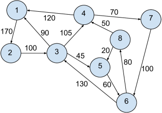
Figure 1: A schematic network with 8 nodes.

For this network, we can compute the resilience margins $\epsilon^{*}_{\infty}$ and $\epsilon^{*}_{1}$, as given in (17) and in (19) for the $\ell_{\infty}$ case and for the $\ell_{1}$ case, respectively; we also computed the perturbation upper limit $\epsilon_{{\mathrm{ub}}}$ as shown in Theorem 6, obtaining

$$\epsilon^{*}_{\infty}=0.0249,\quad\epsilon^{*}_{1}=0.0630,\quad\epsilon_{{\mathrm{ub}}}=0.1878.$$

We next selected 20 evenly spaced values of $\epsilon$ inside the interval $[\epsilon^{*},\epsilon_{{\mathrm{ub}}}]$ and for each of them we computed the worst-case loss as shown in Section 4.1 for the $\ell_{1}$ case and in Section 4.2 for the $\ell_{\infty}$ case. For each value of $\epsilon$, we also modeled a financial shock by generating a random vector of price fluctuation $\delta<0$ such as $\|\delta\|=\epsilon$ and we computed the corresponding loss $\eta^{*}$ by solving Problem 10. We performed 150 runs for each value of $\epsilon$ and in each run we generated a different random vector $\delta$. Figure 2 and Figure 3 show the obtained results for the $\ell_{1}$ case and the $\ell_{\infty}$ case, respectively. The red curve represents the average loss due to random shocks, and the red band represents, for each value of $\epsilon$, the interval between the minimum and maximum losses obtained in the numerical simulation.

It is interesting to observe that the worst-case loss curve presents some “kinks,” i.e., there are $\epsilon$ levels at which the slope of the curve changes abruptly. Intuitively, this feature is due to the change in the group of defaulting banks as the level of perturbation increases. In (25) we have shown that the worst-case price perturbation $\delta^{*}$ in the $\ell_{1}$ case is a vector where the only non-zero component corresponds to the asset $i^{*}$, defined as the one that maximizes $|\zeta_{i}^{\top}\lambda|$. The asset $i^{*}$ is thus the one whose variation causes the worst-case impact. Figure 4 shows the value of $i^{*}$ as function of the perturbation radius $\epsilon$. By comparing Figure 2 and 4, we can observe that the kinks observed in Figure 2 are in correspondence of the changes of values of $i^{*}$.

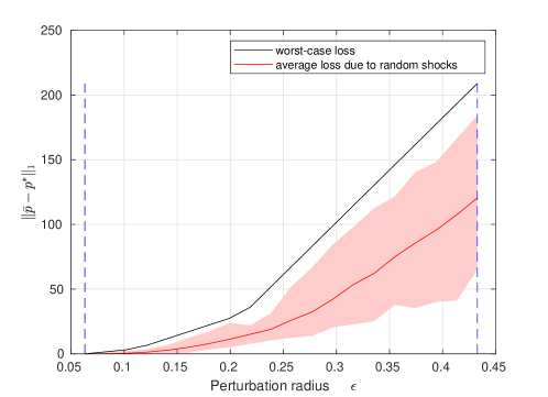
Figure 2: Comparison of the worst-case loss and random shock loss for the $\ell_{1}$ case. The blue dashed lines indicate the resilience margin $\epsilon^{*}$ and the perturbation upper limit $\epsilon_{{\mathrm{ub}}}$.

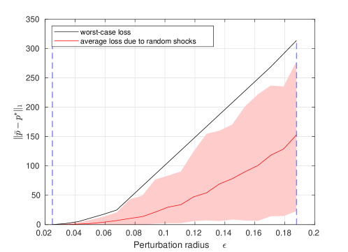
Figure 3: Comparison of the worst-case loss and random shock loss for the $\ell_{\infty}$ case. The blue dashed lines indicate the resilience margin $\epsilon^{*}$ and the perturbation upper limit $\epsilon_{{\mathrm{ub}}}$.

Figure 4: Index $i^{*}$ of the worst-case case perturbation $\delta^{*}$ in the $\ell_{1}$ case. Using Proposition 8, we have checked that $\delta^{*}$ is unique for all $\epsilon>\epsilon^{*}$.

6 Discussion and Conclusions

In this work we considered an extension of the classical financial network model of [18, 16] which includes an additional factor of financial contagion given by the banks’ common exposures in a set of external assets. In this setting, and considering a sign-unrestricted external cash flow $c$, we first provided a characterization of the maximal clearing vector by means of a linear program in Proposition 2. We next introduced in Section 3 the notion of default resilience margin, defined as the maximum tolerable amplitude of assets’ price variation which guarantees that the system remains default-free, and we described how to compute such threshold level in the two relevant cases when the price fluctuations are measured via their maximum amplitude (called the $\ell_{\infty}$ case) or via the sum of their amplitudes (called the $\ell_{1}$ case). These quantities give a clear analytical quantification of the degree of robustness of the financial networks with respect to external assets’ price perturbations. Further, in Section 4 we analyzed what happens when the price perturbation goes beyond the network’s default resilience margin: in this case defaults may appear, and we evaluated the worst-case impact of the perturbation on the total systemic loss of the network. Such worst-case impact, together with a corresponding worst-case price perturbation scenario, can be computed efficiently by solving either a sequence of $m$ linear programs (in the $\ell_{1}$-norm case), or simply one linear program (in the $\ell_{\infty}$-norm case).

It is worth noting that our analysis works for perturbations up to an upper limit $\epsilon_{{\mathrm{ub}}}$ defined and characterized in Section 4.3. Technically, for $\epsilon>\epsilon_{{\mathrm{ub}}}$ perturbations $\delta$ with $\|\delta\|\leq\epsilon$ exist such that the constraint $(\bar{c}+S\delta)+A^{\top}p\geq p$ in problem (21) cannot be satisfied by any $p\geq 0$. In such case, the clearing vector is no longer characterized via the optimal solution of the LP (10). A suitable characterization should instead include constraints of the form $\max((\bar{c}+S\delta)+A^{\top}p,0)\geq p$, which would destroy the convexity of the problem formulation. Also, from a financial perspective, infeasibility of the LP formulation is related to banks’ insolvencies towards the external sector. This may lead to bankruptcy situations which could make the model itself inapt to describe the procedural aspects of firm liquidation and bankruptcy costs [35, 19, 36].

Our model assumes the external assets to be liquid. Financial networks where the institutions have common exposures to illiquid assets are described by more advanced models than the classical Eisenberg-Noe model (see, e.g., [11, 37, 21]) that revise the definition of a clearing vector and take liquidation costs into account. Robustness of such models against external (market-driven) assets’ price fluctuations remains, to the best of our knowledge, an open problem which could be the object of future research. Another important direction of research is to study robustness in presence of defaults and bankruptcy costs [19, 20, 13, 38].

Appendix A Proof of Proposition 1

We begin with some preliminary constructions. A clearing vector may be considered as a fixed point $p=T_{c}(p)$ of the monotone non-decreasing mapping $T_{c}$, defined by the right-hand side of (7)

$$T_{c}:[0,\bar{p}]\to[0,\bar{p}],\quad T_{c}(p)\doteq\min\left(\bar{p},(c+A^{\top}p)^{+}\right)=\left(\min(\bar{p},c+A^{\top}p)\right)^{+}.$$

Since $A$ is a nonnegative matrix, it is easily shown that $T_{c}:[0,\bar{p}]\to[0,\bar{p}]$ is non-decreasing with respect to the ordering $\leq$.

Consider now the following sequence of vectors:

$$p^{0}(c)=\bar{p},\;\;p^{k}(c)=T_{c}(p^{k-1}(c))\in[0,\bar{p}],\quad\forall k\geq 1.$$ (28)

Since $\bar{p}=p^{0}\geq p^{1}$, one has $p^{1}=T_{c}(p^{0})\geq p^{2}=T_{c}(p^{1})$ and, using the induction on $k$, one proves that $p^{k}\geq p^{k+1}$. Also, for each fixed $c$, the map $T_{c}$ is continuous. Passing to the limit as $k\to\infty$, one proves that

$$p^{*}(c)\doteq\lim_{k\to\infty}p^{k}$$

is a fixed point of $T_{c}$, that is, a clearing vector. We have proved that the set of clearing vectors is non-empty.

In order to prove that $p^{*}(c)$ is the maximal clearing vector, consider any other clearing vector $\tilde{p}=T_{c}(\tilde{p})$. Since $p^{0}=\bar{p}\geq\tilde{p}$, one has $p^{1}=T_{c}(p^{0})\geq T_{c}(\tilde{p})=\tilde{p}$ and, using induction, $p^{k}\geq\tilde{p}$ for each $k$. Passing to the limit as $k\to\infty$, one has $p^{*}(c)\geq\tilde{p}$.

Symmetrically, one can notice that the sequence of vectors

$$\tilde{p}^{0}(c)=0,\;\;\tilde{p}^{k}(c)=T_{c}(\tilde{p}^{k-1}(c))\in[0,\bar{p}],\quad\forall k\geq 1.$$

is non-decreasing $\tilde{p}^{k}\leq\tilde{p}^{k+1}$, because $\tilde{p}^{0}\leq\tilde{p}^{1}$. Similar to the previous argument, it can be proved that the limit $p_{*}(c)\doteq\lim_{k\to\infty}\tilde{p}^{k}$ is the minimal clearing vector. $\star$

Appendix B Proof of Proposition 2

Consider the maximal clearing vector $p^{*}(c)$. Notice first that if $c+A^{\top}p^{*}(c)\geq 0$, then the constraints (10) are feasible and satisfied, in fact, by $p=p^{*}(c)$ and by any other clearing vector $p$ such that $c+A^{\top}p\geq 0$. Indeed, every such vector is a solution to (7), which means that $0\leq p\leq\bar{p}$ and $p\leq(c+A^{\top}p)^{+}=c+A^{\top}p$. Since the polyhedron defined by constraints (10) is compact, the LP has a solution. Retracing the proof of Lemma 4 in [18], one shows that each minimizer $p^{*}$ has to be a clearing vector, and thus $p^{*}\leq p^{*}(c)$. Hence, $p^{*}=p^{*}(c)$, otherwise, $p^{*}(c)$ would provide a smaller value of the loss function, which is strictly decreasing in $p$. We have proved that if $c+A^{\top}p^{*}(c)\geq 0$, then the LP (10) is feasible and admits the unique minimizer $p^{*}=p^{*}(c)$.

By noticing that $d^{*}=c+A^{\top}p^{*}(c)$ coincides with the vector (4) of residual values, corresponding to clearing vector $p^{*}(c)$, one proves that all debts to the external sector are paid, if one applies the clearing vector $p^{*}(c)$.

Assume now that LP (7) is infeasible, and hence $c_{i}+(A^{\top}p^{*}(c))_{i}<0$ for some bank $i\in{\cal V}$. Then, for an arbitrary clearing vector $p$ one has $p\leq p^{*}(c)$, and thus $c_{i}+(A^{\top}p)_{i}<0$. This means that bank $i$ is insolvent upon paying its external debts. This finishes the proof. $\star$

Appendix C Proof of Proposition 3

Consider the set $\mathcal{M}=\{(c,p):c\in\mathbb{R}^{m},\,p\in[0,\bar{p}],\,c+A^{\top}p\geq 0\}$. The mapping $\mathfrak{T}(c,p)=T_{c}(p)$ introduced in the proof of Proposition LABEL:prop:min-max-clearing is, as has been proved, non-decreasing (in two arguments) and is element-wise concave, because, for each $i$, the function

$$(c,p)\mapsto\min(\bar{p}_{i},(c+A^{\top}p)_{i}^{+})=\min(\bar{p}_{i},c_{i}+(A^{\top}p)_{i})$$

is concave as the minimum of two concave functions.

By definition, $(c,p^{*}(c))\in\mathcal{M}$ whenever $c\in{\cal C}_{feas}$. In this situation, for every $p\geq p^{*}(c)$, one has $(c,p)\in\mathcal{M}$. In particular, the sequence $p^{k}(c)$ from (28), which is non-increasing and converges to $p^{*}(c)$, satisfies the condition $(c,p^{k}(c))\in\mathcal{M}$ for all $k$ and all $c\in{\cal C}_{feas}$.

We now introduce the mapping $\mathfrak{T}:\mathcal{M}\to[0,\bar{p}]$ defined as $\mathfrak{T}(c,p)\doteq T_{c}(p)$. Obviously, $\mathfrak{T}$ is non-decreasing, that is, $c\leq c^{\prime},p\leq p^{\prime}$ entails that $\mathfrak{T}(c,p)\leq\mathfrak{T}(c^{\prime},p^{\prime})$. Recalling that a composition $f\circ g$ of two non-decreasing concave function $f,g$ is non-decreasing and concave and using induction on $k$, one easily proves now that

$$p^{k}(c)=\mathfrak{T}(c,p^{k-1}(c))$$

is a non-decreasing element-wise concave function of $c\in{\cal C}_{feas}$ for each $k$. Hence, $p^{*}(c)=\lim_{k\to\infty}p^{k}(c)$ is a non-decreasing and element-wise concave function of $c$. The remaining statements about $\eta^{*}$ are now straightforward. $\star$

Appendix D Proof of Theorem 5

Consider the primal problem (10) and let $\alpha\geq 0$, $\beta\geq 0$, $\lambda\geq 0$ be $n$-vectors of Lagrange multipliers. The Lagrangian of this problem is

$${\cal L}={\mathbf{1}}^{\top}(\bar{p}-p)-\alpha^{\top}p+\beta^{\top}(p-\bar{p})+\lambda^{\top}(p-\bar{c}-S\delta-A^{\top}p)$$

and the corresponding dual function is

$$g(\alpha,\beta,\lambda)=\min_{p}\;{\cal L}=\min_{p}\;(\beta+\lambda-{\mathbf{1}}-\alpha-A\lambda)^{\top}p+({\mathbf{1}}-\beta)^{\top}\bar{p}-\lambda^{\top}(\bar{c}+S\delta)$$

Now, $g(\lambda)=-\infty$ whenever the coefficient of $p$ is nonzero, and it is equal to $({\mathbf{1}}-\beta)^{\top}\bar{p}-\lambda^{\top}(\bar{c}+S\delta)$ otherwise. The dual optimization problem is therefore

$$\max_{\alpha,\beta,\lambda\geq 0} ({\mathbf{1}}-\beta)^{\top}\bar{p}-\lambda^{\top}(\bar{c}+S\delta)$$

s.t.: $$\beta+\lambda-{\mathbf{1}}-\alpha-A\lambda=0,$$

or, equivalently, eliminating $\alpha\geq 0$,

$$\max_{\beta,\lambda\geq 0} ({\mathbf{1}}-\beta)^{\top}\bar{p}-\lambda^{\top}(\bar{c}+S\delta)$$

s.t.: $$\beta-{\mathbf{1}}+(I-A)\lambda\geq 0.$$

This dual problem is always strictly feasible, since for any $\lambda\geq 0$ one can always find a sufficiently large $\beta\geq 0$ such that the constraint is satisfied with strict inequality. In such case, strong duality holds (see, e.g., Section 5.2.4 of [26]), hence we have that the optimal objective of the above problem is equal to $\eta^{*}(\delta)$. Therefore, problem (21) can be formulated equivalently as

$$\eta_{{\mathrm{wc}}}=\max_{\|\delta\|\leq\epsilon}\max_{\beta,\lambda\geq 0} \;({\mathbf{1}}-\beta)^{\top}\bar{p}-\lambda^{\top}(\bar{c}+S\delta)$$

s.t.: $$\beta-{\mathbf{1}}+(I-A)\lambda\geq 0.$$

But

$$\max_{\|\delta\|\leq\epsilon}\;({\mathbf{1}}-\beta)^{\top}\bar{p}-\lambda^{\top}(\bar{c}+S\delta)$$

$$\rule{56.9055pt}{0.0pt}=({\mathbf{1}}-\beta)^{\top}\bar{p}-\lambda^{\top}\bar{c}+\max_{\|\delta\|\leq\epsilon}-\lambda^{\top}S\delta$$

$$\rule{56.9055pt}{0.0pt}=({\mathbf{1}}-\beta)^{\top}\bar{p}-\lambda^{\top}\bar{c}-\min_{\|\delta\|\leq\epsilon}\lambda^{\top}S\delta$$

$$\rule{56.9055pt}{0.0pt}=({\mathbf{1}}-\beta)^{\top}\bar{p}-\lambda^{\top}\bar{c}+\epsilon\|S^{\top}\lambda\|_{*},$$

where $\|\cdot\|_{*}$ denotes the dual norm to $\|\cdot\|$. The problem now becomes

$$\eta_{{\mathrm{wc}}}=\max_{\beta,\lambda\geq 0} \;({\mathbf{1}}-\beta)^{\top}\bar{p}-\lambda^{\top}\bar{c}+\epsilon\|S^{\top}\lambda\|_{*}$$

s.t.: $$\beta-{\mathbf{1}}+\lambda-A\lambda\geq 0$$

as claimed. $\star$

Appendix E Proof of Theorem 6

Consider Problem (10), with $c=\bar{c}+S\delta$. For fixed $\epsilon\geq 0$, we have that such problem is feasible for all possible $\delta:\|\delta\|\leq\epsilon$ if and only if there exist $p\geq 0$, $p\leq\bar{p}$ such that $\bar{c}+S\delta+A^{\top}p\geq p$ for all $\delta:\|\delta\|\leq\epsilon$. This latter condition is satisfied if and only if $\min_{\delta:\|\delta\|\leq\epsilon}\bar{c}_{i}+\sigma_{i}^{\top}\delta+(A^{\top}p)_{i}\geq p_{i}$ for all $i=1,\ldots,n$. Computing the minimum on the left-hand side of this expression we have the equivalent conditions $\bar{c}_{i}-\epsilon\|\sigma_{i}^{\top}\|_{*}+(A^{\top}p)_{i}\geq p_{i}$ for all $i=1,\ldots,n$. For finding $\epsilon_{{\mathrm{ub}}}$ we then find the largest $\epsilon$ such that the previous robust feasibility condition is satisfied, which results in the statement of Theorem 6. $\star$

Appendix F On the uniqueness of the worst-case perturbation scenario

We consider a problem of the form

$$\eta_{{\mathrm{wc}}}=\max_{\beta,\lambda} ({\mathbf{1}}-\beta)^{\top}\bar{p}-c_{{\mathrm{wc}}}^{\top}\lambda$$ (29)

s.t.: $$\beta-{\mathbf{1}}+(I-A)\lambda\geq 0$$

$$\beta\geq 0$$

$$\lambda\geq 0.$$

This corresponds to problem (26), by taking $c_{{\mathrm{wc}}}=\bar{c}-\epsilon|S|{\mathbf{1}}$, or to the $i$th subproblem in (24), by taking $c_{{\mathrm{wc}}}=\bar{c}-\epsilon|\zeta_{i}|$. Introduce Lagrange multipliers $p\geq 0$ relative to the first constraint, $v\geq 0$ relative to $\beta\geq 0$, and $w\geq 0$ relative to $\lambda\geq 0$. Then, it is easy to verify that the Lagrangian dual of problem (29) is

$$\eta_{{\mathrm{wc}}}=\min_{p,v,w} {\mathbf{1}}^{\top}(\bar{p}-p)$$ (30)

s.t.: $$p\geq 0$$

$$v= \bar{p}-p\geq 0$$

$$w= c_{{\mathrm{wc}}}-(I-A)^{\top}p\geq 0.$$

Observe that for $\epsilon\leq\epsilon_{{\mathrm{ub}}}$, where $\epsilon_{{\mathrm{ub}}}$ is the insolvency resilience margin, the corresponding worst-case $c$ value used in (30) is such that this LP remains feasible. Therefore, since (30) actually coincides with the LP (10) discussed in Proposition 2 with $c=c_{{\mathrm{wc}}}$, we have that (30) has a unique optimal solution $p^{*}_{{\mathrm{wc}}}$, which represents the clearing vector under the worst-case asset price scenario, in the considered norm. Problem (29) and (30) are dual to each other, and strong duality holds.

We are here concerned with the uniqueness of the optimal solution of problem (29). We next provide a condition for uniqueness which can be tested a posteriori, i.e., after an optimal solution has been computed. Let then such an optimal solution $(\beta^{*},\lambda^{*})$ for problem (29) be given, and let $(p^{*},v^{*},w^{*})$ be the (unique) corresponding optimal solution of the dual problem (30). Define the block matrix $F$ and vector $g$ as

$$F\doteq\left[\begin{array}[]{cc}I&I-A\\ I&0\\ 0&I\end{array}\right],\quad g\doteq\left[\begin{array}[]{c}{\mathbf{1}}\\ 0\\ 0\end{array}\right],\quad$$

so that the constraints in problem (29) are rewritten in compact notation as $F\left[\begin{array}[]{c}\beta\\ \lambda\end{array}\right]\geq g$. Let $Z$ denote the set of row indices in $F$ such that $F_{i}^{\top}\left[\begin{array}[]{c}\beta^{*}\\ \lambda^{*}\end{array}\right]=g_{i}$, where $F_{i}^{\top}$ denotes the $i$th row of $F$, and let $Z=U\cup L$, where $U$ is the set of indices in $i\in Z$ such that $(p^{*},v^{*},w^{*})_{i}>0$, and $L$ is the set of indices in $i\in Z$ such that $(p^{*},v^{*},w^{*})_{i}=0$. Let $F_{U}$, $F_{L}$, $F_{Z}$ denote the submatrices obtained from $F$ by selecting the rows of indices in $U$, $L$ and $Z$, respectively. Consider the LP

$$\iota^{*}=\max_{\beta,\lambda} {\mathbf{1}}^{\top}F_{L}\left[\begin{array}[]{c}\beta\\ \lambda\end{array}\right]$$ (33)

s.t.: $$F_{U}\left[\begin{array}[]{c}\beta\\ \lambda\end{array}\right]=0$$ (36)

$$F_{L}\left[\begin{array}[]{c}\beta\\ \lambda\end{array}\right]\geq 0.$$ (39)

Proposition 7.

Given an optimal solution $(\beta^{*},\lambda^{*})$ for problem (29), construct matrices $F_{U}$, $F_{L}$, $F_{Z}$ and compute the optimal value $\iota^{*}$ of problem (33). The following two conditions are equivalent:

1. $F_{Z}$ has full-column rank and $\iota^{*}=0$;

2. $(\beta^{*},\lambda^{*})$ is the unique optimal solution of problem (29).

This proposition follows from direct application of Theorem 2 and Remark 2 of [34]. We can now derive the following criteria for the uniqueness of the worst-case perturbation scenario that leads to the worst-case loss discussed in Section 4.

Proposition 8 (Uniqueness of the worst-case perturbation scenario).

For the worst-case $\ell_{1}$-norm loss case: the worst-case perturbation scenario in eq. (25) is unique if

• the max in eq. (24) is attained at a single index $i$;

• the corresponding maximization problem in $(\beta,\lambda)$ has a unique solution $(\beta^{*},\lambda^{*})$ (a fact that can be checked by applying Proposition 7);

• $\max_{i}|\zeta_{i}^{\top}\lambda^{*}|$ is attained at a single index $i$.

Similarily, for the worst-case $\ell_{\infty}$-norm loss case: the worst-case perturbation scenario in eq. (27) is unique if

• the maximization problem (26) has a unique solution $(\beta^{*},\lambda^{*})$ (a fact that can be checked by applying Proposition 7);

• $\zeta_{i}^{\top}\lambda^{*}$ is nonzero for all $i$.

References

- \bibcommenthead
- Freixas et al. [2000] Freixas, X., Parigi, B., Rochet, J.-C.: Systemic risk, interbank relations, and liquidity provision by the central bank. Journal of Money, Credit, and Banking 32(3), 611–638 (2000)
- Allen and Gale [2000] Allen, F., Gale, D.: Financial contagion. Journal of Political Economy 108(1), 1–33 (2000)
- Babus [2016] Babus, A.: The formation of financial networks. RAND Journal of Economics 47(2), 239–272 (2016)
- Glasserman and Young [2016] Glasserman, P., Young, H.P.: Contagion in financial networks. Journal of Economic Literature 54(3), 779–831 (2016)
- Hurd [2016] Hurd, T.R.: Contagion! Systemic Risk in Financial Networks. Springer, ??? (2016)
- Acemoglu et al. [2015] Acemoglu, D., Ozdaglar, A., Tahbaz-Salehi, A.: Systemic risk and stability in financial networks. American Economic Review 105(2), 564–608 (2015)
- Nier et al. [2007] Nier, E., Yang, J., Yorulmazer, T., Alentorn, A.: Network models and financial stability. Journal of Economic Dynamics and Control 31(6), 2033–2060 (2007)
- Haldane and May [2011] Haldane, A., May, R.: Systemic risk in banking ecosystems. Nature 469, 351–355 (2011)
- Bardoscia et al. [2017] Bardoscia, M., Battiston, S., Caccioli, F., Caldarelli, G.: Pathways towards instability in financial networks. Nature Communications 8, 14416 (2017)
- Hurd [2023] Hurd, T.R.: Systemic cascades on inhomogeneous random financial networks. Mathematics and Financial Economics 17, 1–21 (2023)
- Cifuentes et al. [2005] Cifuentes, R., Ferrucci, G., Shin, H.S.: Liquidity risk and contagion. Journal of the European Economic Association 3(2-3), 556–566 (2005)
- Allen et al. [2012] Allen, F., Babus, A., Carletti, E.: Asset commonality, debt maturity and systemic risk. Journal of Financial Economics 104(3), 519–534 (2012)
- Banerjee and Feinstein [2022] Banerjee, T., Feinstein, Z.: Pricing of debt and equity in a financial network with comonotonic endowments. Operations Research 70(4), 2085–2100 (2022) https://doi.org/10.1287/opre.2022.2275
- Amini and Feinstein [2023] Amini, H., Feinstein, Z.: Optimal network compression. European Journal of Operational Research 306(3), 1439–1455 (2023) https://doi.org/10.1016/j.ejor.2022.07.026
- Demirer et al. [2021] Demirer, M., Diebold, F.X., Liu, L., Yilmaz, K.: An integrated model for fire sales and default contagion. Mathematics and Financial Economics 15, 59–101 (2021)
- Elsinger et al. [2006] Elsinger, H., Lehar, A., Summer, M.: Risk assessment for banking systems. Management Science 52(9), 1301–1314 (2006)
- Massai et al. [2022] Massai, L., Como, G., Fagnani, F.: Equilibria and systemic risk in saturated networks. Mathematics of Operation Research 47(3), 1707–2545 (2022)
- Eisenberg and Noe [2001] Eisenberg, L., Noe, T.H.: Systemic risk in financial systems. Management Science 47(2), 236–249 (2001)
- Rogers and Veraart [2013] Rogers, L.C., Veraart, L.A.: Failure and rescue in an interbank network. Management Science 59(4), 882–898 (2013)
- Capponi et al. [2016] Capponi, A., Chen, P.-C., Yao, D.D.: Liability concentration and systemic losses in financial networks. Operations Research 64(5), 1121–1134 (2016)
- Feinstein [2017] Feinstein, Z.: Financial contagion and asset liquidation strategies. Operations Research Letters 45(2), 109–114 (2017)
- Banerjee et al. [2019] Banerjee, T., Bernstein, A., Feinstein, Z.: Impact of contingent payments on systemic risk in financial networks. Mathematics and Financial Economics 13, 617–636 (2019)
- Kusnetsov and Veraart [2019] Kusnetsov, M., Veraart, L.A.M.: Interbank clearing in financial networks with multiple maturities. SIAM Journal on Financial Mathematics 10(1), 37–67 (2019)
- Liu and Staum [2010] Liu, M., Staum, J.: Sensitivity analysis of the Eisenberg–Noe model of contagion. Operations Research Letters 38(5), 489–491 (2010)
- Feinstein et al. [2018] Feinstein, Z., Pang, W., Rudloff, B., Schaanning, E., Sturm, S., Wildman, M.: Sensitivity of the Eisenberg–Noe clearing vector to individual interbank liabilities. SIAM Journal on Financial Mathematics 9(4), 1286–1325 (2018)
- Boyd and Vandenberghe [2004] Boyd, S., Vandenberghe, L.: Convex Optimization. Cambridge Univ. Press, New York (2004)
- Csóka and Herings [2021] Csóka, P., Herings, P.J.-J.: An axiomatization of the proportional rule in financial networks. Management Science 67(5), 2799–2812 (2021)
- Thomson [2013] Thomson, W.: Game-theoretic analysis of bankruptcy and taxation problems: Recent advances. International Game Theory Review 15(03), 1340018 (2013)
- Moreno-Ternero [2009] Moreno-Ternero, J.D.: The proportional rule for multi-issue bankruptcy problems. Economics Bulletin 29(1), 474–481 (2009)
- Csóka and Jean-Jacques Herings [2018] Csóka, P., Jean-Jacques Herings, P.: Decentralized clearing in financial networks. Management Science 64(10), 4681–4699 (2018)
- Calafiore et al. [2021] Calafiore, G.C., Fracastoro, G., Proskurnikov, A.V.: On optimal clearing payments in financial networks. In: IEEE Conf. Decision and Control, pp. 4804–4810 (2021)
- Calafiore et al. [2024] Calafiore, G.C., Fracastoro, G., Proskurnikov, A.V.: Optimal clearing payments in a financial contagion model. SIAM Journal on Financial Mathematics (accepted) (2024). available online as ArXiv:2103.10872v2
- Ren and Jiang [2016] Ren, X., Jiang, L.: Mathematical modeling and analysis of insolvency contagion in an interbank network. Operations Research Letters 44(6), 779–783 (2016)
- Mangasarian [1979] Mangasarian, O.L.: Uniqueness of solution in linear programming. Linear Algebra and its Applications (25), 151–162 (1979)
- Elsinger [2009] Elsinger, H.: Financial Networks, Cross Holdings, and Limited Liability. Oesterreichische Nationalbank Austria, Wien, Austria (2009). Working Papers 156
- Weber and Weske [2017] Weber, S., Weske, K.: The joint impact of bankruptcy costs, fire sales and cross-holdings on systemic risk in financial networks. Probability, Uncertainty and Quantitative Risk 2, 9 (2017)
- Amini et al. [2016] Amini, H., Filipović, D., Minca, A.: To fully net or not to net: Adverse effects of partial multilateral netting. Operations Research 64(5), 1135–1142 (2016)
- Ararat and Meimanjan [2023] Ararat, C., Meimanjan, N.: Computation of systemic risk measures: A mixed-integer programming approach. Operations Research 71(6), 2130–2145 (2023)