Process-and-Forward: Deep Joint Source-Channel Coding Over Cooperative Relay Networks

Abstract

This paper introduces an innovative deep joint source-channel coding (DeepJSCC) approach to image transmission over a cooperative relay channel. The relay either amplifies and forwards a scaled version of its received signal, referred to as DeepJSCC-AF, or leverages neural networks to extract relevant features about the source signal before forwarding it to the destination, which we call DeepJSCC-PF (Process-and-Forward). In the full-duplex scheme, inspired by the block Markov coding (BMC) concept, we introduce a novel block transmission strategy built upon novel vision transformer architecture. In the proposed scheme, the source transmits information in blocks, and the relay updates its knowledge about the input signal after each block and generates its own signal to be conveyed to the destination. To enhance practicality, we introduce an adaptive transmission model, which allows a single trained DeepJSCC model to adapt seamlessly to various channel qualities, making it a versatile solution. Simulation results demonstrate the superior performance of our proposed DeepJSCC compared to the state-of-the-art BPG image compression algorithm, even when operating at the maximum achievable rate of conventional decode-and-forward and compress-and-forward protocols, for both half-duplex and full-duplex relay scenarios.

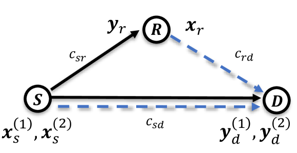
(a) Half-duplex relaying: The solid arrows denote the transmission in the relay-receive period while the dashed ones represent that in the relay-transmit period.

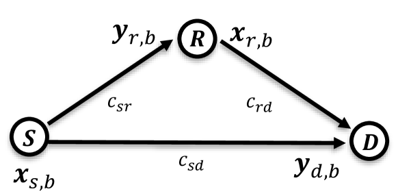
(b) Full-duplex relaying: The relay can receive and transmit simultaneously.

Figure 1: Illustrations of the half-duplex and full-duplex relay channels.

I Introduction

Cooperative communications empower nodes within a network to harness their neighboring nodes’ resources, enhancing spectral efficiency and fortifying the network against channel fading [2]. One of the fundamental cooperative communication models is the relay channel, comprising three key elements: the source, the relay, and the destination, as depicted in Fig. 1. The source transmits its message to both the relay and the destination. The relay processes the received signal and transmits it to the destination, while the destination tries to recover the original message by combining the signals received from both the source and the relay.

Three classical relaying protocols are commonly employed: amplify-and-forward (AF), decode-and-forward (DF), and compress-and-forward (CF) [3, 4, 5, 6, 7, 8, 9]. In AF, the relay straightforwardly scales and forwards its received signal to the destination, albeit it is constrained by the drawback of noise forwarding. In DF, on the other hand, the relay decodes the received signal before re-encoding and forwarding it. While DF mitigates the noise forwarding issue, it faces limitations when the source-to-relay channel quality is subpar. CF adopts a different approach, having the relay compress its received signal using Wyner-Ziv source coding [10], while treating the destination’s received signal as side information. Despite many efforts, the capacity of a general relay channel could not be characterized in a single-letter form.

Remarkably, it has been demonstrated in [11] that separate compression followed by cooperative channel coding is optimal under infinite source and channel block lengths, even though the capacity of the relay channel’s capacity cannot be computed accurately. However, in practical finite block length regimes, joint source-channel coding (JSCC) often outperforms the separation approach, though there is limited research on JSCC applied to relay channels. The study in [11] delves into JSCC within cooperative relay networks from an information-theoretic perspective. Additionally, JSCC for cooperative multimedia source transmission has been explored in [12, 13]. These papers primarily focus on designing separate codes for compression and error correction, optimizing their parameters jointly to bolster resilience against channel variations.

More recently, deep learning (DL) has made significant strides in addressing various communication challenges, particularly in the realm of JSCC. The DeepJSCC scheme introduced in [14] has demonstrated superiority over conventional digital approaches, combining state-of-the-art compression techniques with nearly optimal channel codes for image transmission across AWGN and Rayleigh fading channels. Moreover, it exhibits graceful degradation as channel quality weakens. Recognizing the great potential of DeepJSCC, researchers are actively extending DeepJSCC framework to different wireless communication channels [15]. For instance, the authors in [16] show the compatibility of DeepJSCC with the OFDM scheme to combat with the multipath fading channel, [17] introduces the self attention module which enables SNR-adaptive transmission using a single model. In [18, 19, 20, 21], the DeepJSCC framework is applied to video, audio and point cloud sources, highlighting it as an effective tool for a large variety of applications.

Despite these notable advances in applying DeepJSCC in critical scenarios, prior work has primarily concentrated on point-to-point channels, leaving the more intricate multi-user scenarios largely unexplored. Notably, the authors in [22] delve into a multiple access channel with two users communicating with the receiver under the DeepJSCC framework. DeepJSCC is also applied to image transmission over the broadcast [23] and the multi-hop relay channels [24, 25, 26]. However, when it comes to cooperative communications, there appears to be a significant gap in research. The most relevant work [27] considers the three-node cooperative relay channel yet it is specifically designed for speech and focus on energy efficient transmission. Our previous work [1] is the first to investigate image transmission over the half-duplex relay channel. However, the considered scenario in [1] is limited as it assumes that the source node keeps silent in the relay-transmit period. This motivates us to embark on the journey of realizing DeepJSCC within more general cooperative relay networks for image transmission.

In this paper, we introduce the first DeepJSCC framework tailored for both the half-duplex and full-duplex relay channels. Within this framework, we present two distinctive relaying protocols: DeepJSCC-AF and DeepJSCC-PF. These protocols draw parallels with the classical AF and DF schemes and are designed to operate effectively in both half-duplex and full-duplex relay scenarios. In the DeepJSCC-AF protocol, the relay simply amplifies its received signal while adhering to power constraints. On the other hand, DeepJSCC-PF involves signal processing at the relay using deep neural networks (DNNs). These DNNs are jointly optimized with the DNNs at the source and destination nodes to achieve superior reconstruction performance. The inspiration for the DeepJSCC-PF protocol is rooted in the principles of the traditional DF protocol, although there is no decoding in the strict sense since DeepJSCC does not rely on digital encoding of information, and hence, the source signal cannot be decoded accurately. We meticulously search for the optimal parameters to enhance the performance in the half-duplex relay, while applying a block-based transmission strategy inspired by the well-known block Markov coding (BMC) in the full-duplex scenario.

Our dedicated experiments unequivocally demonstrate the effectiveness of the proposed DeepJSCC-PF protocol in both half-duplex and full-duplex scenarios. To enhance the practicality of these DeepJSCC schemes, particularly in the context of full-duplex relay, we move beyond training separate models for varying channel/link conditions. Instead, we propose a single adaptive model that leverages link conditions as side information to attain reconstruction performance on par with individually trained models.

The main contributions of this paper can be summarized as follows:

• We present a novel DeepJSCC framework for both the half-duplex and full-duplex relay channels, under which two protocols, DeepJSCC-AF and DeepJSCC-PF, are proposed. We propose a novel transformer-based coding architecture built upon the vision transformer (ViT) [28] to parameterize encoding and decoding functions at the source, relay, and destination nodes, resulting in exceptional reconstruction performance.

• We provide a thorough overview of existing approaches in digital communications, serving as the foundation for the development of our DeepJSCC schemes. Specifically, our DeepJSCC-PF protocol for full-duplex relay is inspired by the BMC scheme used in the conventional DF protocol. To the best of our knowledge, it is the first time a practical block-based cooperative coding scheme is proposed in the JSCC context. We highlight the distinctions and challenges encountered in designing our DeepJSCC-PF scheme.

• We introduce a link quality adaptation (LA) module to create a flexible framework that can adapt to varying link qualities in full-duplex relay scenarios. This module adjusts transmitted signals based on different link qualities, enabling us to achieve reconstruction performance comparable to separately trained models using a single adaptive model.

• Extensive numerical experiments conducted in both half-duplex and full-duplex relay settings to showcase the advantages offered by the proposed protocols over the digital baseline. The baseline employs the BPG image compression algorithm and communicates at the maximum rate achievable by the DF and CF protocols. Furthermore, we demonstrate that our proposed schemes effectively mitigate both the cliff and leveling effects.

Throughout the paper, scalars are represented by normal-face letters (e.g., $x$), while uppercase letters (e.g., $X$) represent random variables. Matrices and vectors are denoted by bold upper and lower case letters (e.g., $\bm{X}$ and $\bm{x}$), respectively. A set is denoted by the double stroke font, e.g., $\mathbb{S}$. Transpose and Hermitian operators are denoted by $(\cdot)^{\top}$, $(\cdot)^{\dagger}$, respectively. We utilize $\bm{x}_{1:b}$ to index the first $b$ elements of a vector $\bm{x}$.

II System model

We consider a classical relay channel model consisting of a source node $\mathrm{S}$, a destination node $\mathrm{D}$, and a relay node $\mathrm{R}$, as illustrated in Fig. 1. The goal is to deliver an image $\bm{S}\in\mathbb{R}^{C\times H\times W}$ from $\mathrm{S}$ to $\mathrm{D}$ with the help of relay $\mathrm{R}$, where $C$, $H$, $W$ denote the number of color channels, the height and width of the image, respectively. The relay node $\mathrm{R}$ can operate in either the half-duplex mode or the full-duplex mode.

II-A Half-Duplex Relaying

In the half-duplex mode, the relay cannot receive and transmit at the same time, as shown in Fig. 1(a). Thus, the transmission is divided into two periods [4]: the relay-receive and relay-transmit periods, occupying $\alpha$ and $(1-\alpha)$ proportion of the overall transmission duration, respectively. The parameter $\alpha$ is termed the “time-division variable”, signifying its role in determining the temporal allocation of relay operations.

At the beginning of transmission, the source node $\mathrm{S}$ encodes the image $\bm{S}$ into a channel codeword $\bm{x}_{s}\in\mathbb{C}^{k}$:

$$\bm{x}_{s}=f_{s}(\bm{S}),$$ (1)

where $f_{s}(\cdot):\mathbb{R}^{C\times H\times W}\rightarrow\mathbb{C}^{k}$ is an encoding function, and $\bm{x}_{s}$ is subject to an average power constraint:

$$\frac{1}{k}\|\bm{x}_{s}\|^{2}_{2}\leq P_{s}.$$ (2)

The codeword $\bm{x}_{s}$ can be partitioned into two parts: $\bm{x}_{s}=\begin{bmatrix}\bm{x}_{s}^{(1)}\\ \bm{x}_{s}^{(2)}\end{bmatrix}$ with $\bm{x}_{s}^{(1)}\in\mathbb{C}^{\alpha k}$ for the relay-receive period and $\bm{x}_{s}^{(2)}\in\mathbb{C}^{(1-\alpha)k}$ for the relay-transmit period.

In the relay-receive period, $\mathrm{S}$ transmits $\bm{x}_{s}^{(1)}$ to both $\mathrm{R}$ and $\mathrm{D}$. The signals received at $\mathrm{R}$ and $\mathrm{D}$ are denoted by $\bm{y}_{r}$ and $\bm{y}_{d}^{(1)}$, respectively, which can be written as

$$\bm{y}_{r}=c_{sr}\bm{x}_{s}^{(1)}+\bm{n}_{r},$$ (3)

$$\bm{y}_{d}^{(1)}=c_{sd}\bm{x}_{s}^{(1)}+\bm{n}_{d}^{(1)},$$ (4)

where $c_{sr}$, $c_{sd}$ are real constants governed by the transmission distances of the $\mathrm{S}$-$\mathrm{R}$ and $\mathrm{S}-\mathrm{D}$ links, respectively; $\bm{n}_{r}$ and $\bm{n}_{d}^{(1)}$ denote the independent complex additive white Gaussian noise (AWGN) terms, and without loss of generalizability, we assume $\bm{n}_{r},\bm{n}_{d}^{(1)}\sim\mathcal{CN}(\bm{0},\bm{I}_{\alpha k})$, where $\bm{I}_{\alpha k}$ denotes identity matrix with dimension $\alpha k\times\alpha k$.

Upon receiving $\bm{y}_{r}$, the relay re-encodes it by

$$\bm{x}_{r}=f_{r}(\bm{y}_{r}),$$ (5)

where $f_{r}(\cdot):\mathbb{C}^{\alpha k}\rightarrow\mathbb{C}^{(1-\alpha)k}$ is the re-encoding function, and $\bm{x}_{r}\in\mathbb{C}^{(1-\alpha)k}$ is subject to a power constraint:

$$\frac{1}{k}\|\bm{x}_{r}\|^{2}_{2}\leq P_{r}.$$ (6)

This power constraint ensures that the total energy transmitted by the relay is the same for different $\alpha$ values.

In the relay-transmit period, the relay forwards $\bm{x}_{r}$ to the destination, and the signal received at the destination can be written as:

$$\bm{y}_{d}^{(2)}=c_{rd}\bm{x}_{r}+c_{sd}\bm{x}_{s}^{(2)}+\bm{n}_{d}^{(2)},$$ (7)

where $c_{rd}$ is the real channel gain for the R-D link and each element in $\bm{n}_{d}^{(2)}$ is independent and follows a complex Gaussian distribution with zero mean and unit variance.

Given the received signal $\bm{y}_{d}=\begin{bmatrix}\bm{y}_{d}^{(1)}\\ \bm{y}_{d}^{(2)}\end{bmatrix}\in\mathbb{C}^{k}$ over the two periods, the destination aims to reconstruct the image using a decoding function $g(\cdot):\mathbb{C}^{k}\rightarrow\mathbb{R}^{C\times H\times W}$. The reconstructed image is given by

$$\hat{\bm{S}}=g(\bm{y}_{d}).$$ (8)

II-B Full-Duplex Relaying

In contrast to half-duplex replaying, the relay can receive and transmit at the same time in the full-duplex mode. Following [29, 4], we consider block transmission: the data transmissions among $\mathrm{S}$, $\mathrm{R}$, and $\mathrm{D}$ occur in a block-wise fashion, and each block transmission occupies one time slot.

To start with, the source node $\mathrm{S}$ encodes the image to $\bm{x}_{s}=f_{s}(\bm{S})$ and equally partitions $\bm{x}_{s}$ to $B$ blocks, yielding $\bm{x}_{s}=[\bm{x}_{s,1}^{\top},\ldots,\bm{x}_{s,B}^{\top}]^{\top}$, where $\bm{x}_{s,b}\in\mathbb{C}^{{k}/{B}}$. The same power constraint in (2) is also imposed on $\bm{x}_{s}$.

The encoded blocks will be transmitted in $B$ slots. In the $b$-th time slot, the source transmits $\bm{x}_{s,b}$ to both the relay and the destination. At the relay, the received signal $\bm{y}_{r,b}$ can be written as

$$\bm{y}_{r,b}=c_{sr}\bm{x}_{s,b}+\bm{n}_{r,b},$$ (9)

where $\bm{n}_{r,b}\sim\mathcal{CN}({\bm{0},\bm{I}_{{k}/{B}}})$. For the same time slot, the relay node generates and transmits $\bm{x}_{r,b},b>1$, based on all the previously received signals,

$$\bm{x}_{r,b}=f_{r}(\bm{y}_{r,1:(b-1)}),$$ (10)

where $\bm{y}_{r,1:(b-1)}\triangleq\{\bm{y}_{r,1},\cdots,\bm{y}_{r,(b-1)}\}$.

Denote by $\bm{x}_{r}=[\bm{x}_{r,1}^{\top},\cdots,\bm{x}_{r,B}^{\top}]^{\top}$ all the signals transmitted by the relay, the power constraint at the relay is $\frac{1}{k}\mathbb{E}(\bm{x}_{r}^{\dagger}\bm{x}_{r})\leq P_{r}$.

The $b$-th transmitted block from the source and the relay are superimposed at the destination node:

$$\bm{y}_{d,b}=c_{sd}\bm{x}_{s,b}+c_{rd}\bm{x}_{r,b}+\bm{n}_{d,b},$$ (11)

where $\bm{n}_{d,b}\sim\mathcal{CN}({\bm{0},\bm{I}_{{k}/{B}}})$. After collecting all the received blocks, $\bm{y}_{d}\triangleq[\bm{y}_{d,1}^{\top},\cdots,\bm{y}_{d,B}^{\top}]^{\top};\bm{y}_{d}\in\mathbb{C}^{k}$, a decoding function, $g(\cdot)$ is used to reconstruct the original image $\hat{\bm{S}}$. The peak signal-to-noise ratio (PSNR) and the structural similarity index (SSIM) are used to evaluate the reconstruction quality, the PSNR is defined as:

$$\text{PSNR}=10\log_{10}\frac{255^{2}}{\frac{1}{M}||\bm{S}-\hat{\bm{S}}||^{2}_{F}},$$ (12)

where $M=CHW$ denotes the total number of pixels of the image $\bm{S}$. The SSIM is given as:

$$\text{SSIM}=\frac{(2\mu_{s}\mu_{\hat{s}}+c_{1})(2\sigma_{s\hat{s}}+c_{2})}{(\mu^{2}_{s}+\mu^{2}_{\hat{s}}+c_{1})(\sigma^{2}_{s}+\sigma^{2}_{\hat{s}}+c_{2})},$$ (13)

where $\mu_{s},\sigma_{s},\sigma_{s\hat{s}}$ are the mean and variance of $\bm{S}$, and the covariance between $\bm{S}$ and $\hat{\bm{S}}$, respectively. $c_{1}$ and $c_{2}$ are constants for numeric stability. Note that for both half-duplex and full-duplex relay, we adopt the ‘bandwidth ratio’ to quantify the available (complex) channel use per pixel (CPP), defined as $\rho\triangleq\frac{k}{M}$.

III DeepJSCC-based Half-Duplex Relaying

In this section, we propose two protocols adopting DeepJSCC over the half-duplex relay channel, namely, the DeepJSCC-AF and DeepJSCC-PF. In both protocols, we parameterize the encoder $f_{s}(\cdot)$, decoder $g(\cdot)$, and the transformations $f_{r}(\cdot)$ at the relay by DNNs.

III-A Recap of ViT models

Before delving into the details of the proposed relaying protocols, we provide a quick overview of the encoding and decoding processes using ViT models, which form the core foundation of our approach.

III-A1 ViT encoder

As shown in the left hand side of Fig. 2, the ViT encoder is comprised of three parts: image-to-sequence transformation, self-attention, and linear projection.

Image-to-sequence transformation. We evenly partition the input image $\bm{S}$ into a sequence of $p\times p$ tokens along its spatial dimensions, where each token consists of ${M}/{p^{2}}$ elements. The tokens are further processed by a multilayer perceptron (MLP) layer with Gaussian error linear unit (GeLU) activation function with an output of dimension $c$.

Self-attention module. After obtaining the $p^{2}$ tokens, the same positional embedding technique in [28] is adopted to provide additional positional information, and organize the positionally embedded tokens into a matrix $\bm{S}_{e}\in\mathbb{R}^{p^{2}\times c}$. Then, $N_{e}$ transformer layers are stacked together and applied to $\bm{S}_{e}$ to generate the output $\widetilde{\bm{S}}_{e}$. As an example, we illustrate the operations of the first transformer layer as follows:

$$\bm{S}_{1} =\bm{S}_{e}+\text{MSA}(\bm{S}_{e}),$$

$$\bm{S}_{2} =\bm{S}_{1}+\text{MLP}(\text{LN}(\bm{S}_{1})),$$ (14)

where $\text{MSA}(\cdot)$ denotes the multi-head self-attention layer [30], $\text{LN}(\cdot)$ represents layer norm operation and MLP is comprised of linear layers with GeLU activation function. Note that $\bm{S}_{2}$ will be further fed into the subsequent transformer layers.

Linear Projection. After passing $N_{e}$ transformer layers, we apply a linear layer to the output matrix $\widetilde{\bm{S}}_{e}$ (or $\widetilde{\bm{S}}^{\prime}_{e}$ if LA module is adopted for adaptive transmission introduced in Section IV-D) with dimensions $p^{2}\times c$, and map it to the output matrix $\bm{X}\in\mathbb{R}^{p^{2}\times c^{*}}$, where $p^{2}c^{*}=2k$ and $k$ is the number of complex channel uses.

III-A2 ViT decoder

The ViT decoding process mirrors ViT encoding. As shown in the right hand side of Fig. 2, the ViT decoder is also comprised of three modules: linear projection, self-attention, and sequence-to-image transformation. If we denote the noisy channel output by $\bm{Y}\in\mathbb{R}^{p^{2}\times c^{*}}$, which is fed into the ViT decoder, the linear projection module maps each token of $\bm{Y}$ to a $c$-dimensional vector, which will be positionally embedded to form a matrix $\bm{S}_{d}\in\mathbb{R}^{p^{2}\times c}$ and further processed by the subsequent $N_{d}$ transformer layers. An MLP with GeLU activation function is applied to the final output of the self-attention modules $\widetilde{\bm{S}}_{d}$ ($\widetilde{\bm{S}}^{\prime}_{d}$ if LA module is adopted) to generate a matrix with dimensions $p^{2}\times\frac{M}{p^{2}}$. Finally, the patch re-arrange layer is responsible for converting this matrix back to the reconstructed image $\hat{\bm{S}}\in\mathbb{R}^{C\times H\times W}$.

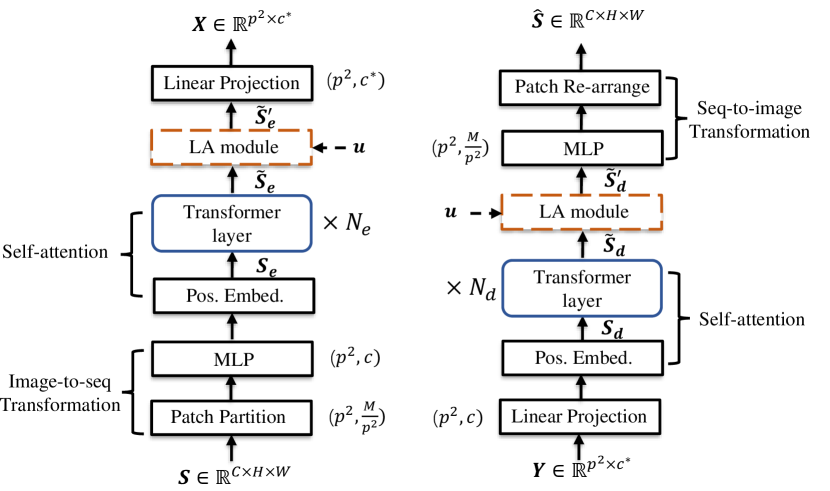
Figure 2: The neural network architecture of the ViT encoder (left) and decoder (right). The (optional) ‘LA module’ which takes the side information $\bm{u}$ as an additional input is adopted for the adaptive transmission model introduced in Section IV.

III-B Relaying Protocols

This subsection introduces the proposed DeepJSCC-based relaying protocols. We will provide an in-depth exploration of the DNN structures tailored specifically to accommodate and execute these protocols seamlessly.

III-B1 DeepJSCC-AF

We first consider a simple relaying protocol, where the relay transmits a scaled version of its received signal:

$$\bm{x}_{r}=\eta\bm{y}_{r},$$ (15)

where $\eta$ is chosen to satisfy the power constraint. Note that, in the DeepJSCC-AF protocol, to ensure the relay participates in the whole transmission process for better performance, we set $\alpha=1/2$ such that the transmitted signal $\bm{x}_{r}\in\mathbb{C}^{(1-\alpha)k}$ is of the same length with that of $\bm{y}_{r}\in\mathbb{C}^{\alpha k}$. Then, $\eta$ can be calculated as $\eta=\sqrt{\frac{2P_{r}}{P_{s}^{(1)}c_{sr}^{2}+1}}$, where $2$ corresponds to $\alpha=1/2$ and $P_{s}^{(1)}$ denotes the source transmit power in the relay-receive period.

At the receiver, we have the received signal in the relay-receive period, $\bm{y}_{d}^{(1)}$, and that in the relay-transmit period, $\bm{y}_{d}^{(2)}=c_{rd}\bm{x}_{r}+c_{sd}\bm{x}_{s}^{(2)}+\bm{n}_{d}^{(2)}$, where $\bm{n}_{d}^{(2)}\sim\mathcal{CN}(\bm{0},\bm{I}_{k/2})$. The entire received signal, $\bm{y}_{d}$, at the receiver is converted into a real vector, reshaped to $\bm{Y}\in\mathbb{R}^{p^{2}\times c^{*}}$, and fed to the DeepJSCC-AF decoder parameterized by the aforementioned ViT decoder to generate the reconstructed image $\hat{\bm{S}}$.

III-B2 DeepJSCC-PF

DeepJSCC-AF suffers from noise propagation since the relay merely transmits a scaled version of the received noisy signal. In the realm of digital communications, more sophisticated relaying schemes, such as DF and partial DF (pDF) [5], address this issue. In particular, the DF (pDF) protocol decodes the original message (or part of it) getting rid of the noise and only relevant information is relayed to the destination. Denoising the received signal at the relay is challenging in the context of DeepJSCC-based schemes, which directly map the source information to continuous amplitude symbols. Inherently, complete denoising will not be possible in DeepJSCC, which renders both the DF and pDF schemes infeasible.

Another well-known cooperation scheme, CF [3, 8], involves the relay compressing its received signal treating the destination’s received signal as correlated side information. Wyner-Ziv coding is then used to compress the relay’s received signal, whose index is forwarded to the destination using an independent channel code. In addition to the suboptimality of this separation-based approach in the finite block length regime, the compression scheme at the relay is also oblivious to the underlying channel code. In general, it is also possible to combine pDF and CF into the partial decode-compress-and-forward (pDCF) scheme [9].

In an attempt to combine the benefits of the conventional pDF and CF protocols in the context of DeepJSCC, we introduce DeepJSCC-PF. In this scheme, we parameterize the relay’s processing function $f_{r}(\cdot)$ by a modified ViT encoder. It is worth noting that, unlike the source encoder, which receives an image as the input, there is no need for a patch partition layer in the modified ViT encoder at the relay, whose input is the received noisy channel output. The underlying idea here is to craft a relay protocol that undergoes automatic optimization through end-to-end training, ultimately aiming for superior reconstruction performance. This approach allows us to break away from the limitations of conventional methods and adapt our relaying strategy to the specific needs of the source data, enhancing its overall effectiveness.

Following the intuition, the overall encoding, relay processing and decoding procedure can be summarized as follows: the ViT encoder at the source node generates $\bm{X}\in\mathbb{R}^{p^{2}\times c^{*}}$ as shown in Fig. 1. Then, we partition it into two parts along the column for relay-receive and relay-transmit periods as $\bm{X}=[\bm{X}^{(1)},\bm{X}^{(2)}]$ where each column of $\bm{X}^{(1)}$ and $\bm{X}^{(2)}$ is of $\alpha c^{*}$ and $(1-\alpha)c^{*}$ dimension, respectively. The received signal at the relay, $\bm{y}_{r}$ is first converted to a real vector and reshaped into $\bm{Y}_{r}$ with dimensions $p^{2}\times\alpha c^{*}$. A linear projection layer maps each token of $\bm{Y}_{r}$ to a $c$-dimensional vector followed by a positional embedding layer to form a new matrix that will be fed to $N_{r}$ consecutive transformer layers. Notice that the relay output is a complex vector of length-$(1-\alpha)k$, thus, the final linear projection layer will map each $c$-dimensional input token to a $(1-\alpha)c^{*}$-dimensional vector.

For both protocols, we adopt the mean square error (MSE) as the loss function:

$$\mathcal{L}=\mathbb{E}_{\bm{S}\sim p(\bm{S})}\left[\|\bm{S}-\hat{\bm{S}}\|^{2}_{F}\right].$$ (16)

III-C Important variables

For digital cooperative communications, when the link qualities $(c_{sr},c_{rd},c_{sd})$ and the transmission power $(P_{s},P_{r})$ are given, some variables, such as the time division variable $\alpha$, the power allocation variable $\gamma$, and the correlation variable $\beta$ (for DF protocol), are critical in determining the achievable rate. The conventional schemes aim to maximize the achievable rate, which necessitates the optimization of these aforementioned variables [4]. In this section, our intention is to highlight these variables, recognizing their pivotal role in influencing system performance. Later in the simulation results, we will demonstrate how the DNNs can autonomously learn to optimize these variables, ultimately leading to an efficient end-to-end image reconstruction process.

First, the time division variable $\alpha$ introduced in Section II divides the time for relay transmit period and relay receive period. Second, the power allocation variable $\gamma$ defined as below determines the average transmission power at the two periods, $P_{s}^{(1)}$ and $P_{s}^{(2)}$, defined as:

$$\gamma\triangleq\frac{\mathbb{E}{\|\bm{x}_{s}^{(1)}\|^{2}_{2}}}{\mathbb{E}{\|\bm{x}_{s}\|^{2}_{2}}},$$ (17)

which leads to $P_{s}^{(1)}=\frac{\gamma P_{s}}{\alpha}$ and $P_{s}^{(2)}=\frac{(1-\gamma)P_{s}}{1-\alpha}$. Finally, we introduce the correlation variable $\beta$ as follows. Consider the conventional pDF protocol where the source aims to convey an index $w\in[1,2^{nR}]$ to the destination, it first splits it into sub-indexes $w_{1}$ and $w_{2}$, which will be further encoded for transmission. To be precise, at the relay-receive period, the source encodes $w_{1}$ to $\bm{x}^{(1)}_{s}(w_{1})$ with power $P_{s}^{(1)}$ which is broadcasted to both the relay and the destination. Following the DF protocol, the relay receives the message, decodes the index $w_{1}$ and re-encodes it to $\bm{x}_{r}=\bm{x}_{r}(w_{1})$ which is power normalized under the constraint $P_{r}$. The source signal, $\bm{x}_{s}^{(2)}=\bm{x}_{s}^{(2)}(w_{1},w_{2})$ at the relay-transmit period is comprised of two independent parts, $\bm{x}_{r}(w_{1})$ and $\bm{x}_{s}^{(2)}(w_{2})$, which are superimposed for transmission. The first term is identical to the relay transmitted signal (up to a scaling factor) whose power is $\beta P_{s}^{(2)}$ while the second term conveys distinct message $w_{2}$ and is independent of the first term with power $(1-\beta)P_{s}^{(2)}$. Following the above definitions, the correlation variable is given by

$$\beta=\frac{\mathbb{E}{(\bm{x}_{r}^{\dagger}\bm{x}_{s}^{(2)}})}{\sqrt{\mathbb{E}{\|\bm{x}_{s}^{(2)}\|^{2}_{2}}\mathbb{E}{\|\bm{x}_{r}\|^{2}_{2}}}}.$$ (18)

Intuitively, the $\beta$ value indicates the ‘correlation’ between the relay transmit signal and the source transmit signal in the relay-transmit period. As long as the relay correctly decodes the index $w_{1}$, having a non-zero $\beta$ value allows the coherent superposition between the signal from the source and that from the relay to boost their power against the noise providing stronger error correction ability for $w_{1}$. However, a large $\beta$ value implies the source may no longer be capable to reliably transmit the new information $w_{2}$ to the destination resulting in a rate loss. Thus, it is important to figure out a good $\beta$ to balance the transmission for $w_{1}$ and $w_{2}$.

In our DeepJSCC scheme, however, there is no concept of indexes, $w_{1}$ and $w_{2}$, since we adopt the analogy transmission. It is impossible to figure out the optimal parameters analytically as in the case of [4], instead, for each link quality and transmit power, we will first determine an optimal $\alpha^{*}$ from a discrete set and then let the neural network to automatically figure out the corresponding $\beta$ and $\gamma$ for that $\alpha^{*}$. As will be shown in the simulation part, by analyzing the variables $\alpha,\beta,\gamma$, we can gain more insights on the end-to-end optimized DeepJSCC-PF model for the half-duplex relay.

TABLE I: Block Markov coding with $B$ blocks.

$b$	1	2	…	$B-1$	$B$
$\mathrm{S}$	$\bm{x}_{s}(m_{1}|1)$	$\bm{x}_{s}(m_{2}|m_{1})$	…	$\bm{x}_{s}(m_{B-1}|$ $m_{B-2})$	-
$\mathrm{R}$	-	$\bm{x}_{r}(\tilde{m}_{1})$	…	$\bm{x}_{r}(\tilde{m}_{B-2})$	$\bm{x}_{r}(\tilde{m}_{B-1})$

IV DeepJSCC-based Full-Duplex Relaying

In this section, we delve into the realm of full-duplex relaying. We shall elucidate the means by which enhanced performance can be realized when the relay possesses the capability to receive and transmit simultaneously.

IV-A Block Markov Coding (BMC)

To develop full-duplex relaying protocols within the DeepJSCC scheme, let us begin by revisiting the traditional DF protocol for full-duplex relays, which is known as BMC [3]. This initial step will help us gain a better understanding of the concept.

In the BMC framework, both the source and the relay collaborate to transmit a message to the destination over a span of $B$ blocks. Only after receiving the entire signal, the receiver decodes the information of all the blocks, which is known as backward decoding [3, 6].

IV-A1 Block Markov encoding

Assume a joint distribution $p(X_{s},X_{r})$, where $X_{s}$ denotes the random channel input of the source, while $X_{r}$ denotes that at the relay. The source wants to transmit $(B-1)$ messages, $m_{j}\in[1,2^{nR}],j\in[1,B-1]$ over $B$ blocks, where $n$ denotes the number of real channel uses for each block and $R$ denotes the code rate. At the end of the $b$-th block, $b\in[2,B]$, the relay decodes the message $m_{b}$ from the received signal $\bm{y}_{r,b}$ at the $b$-th block by finding the message $\tilde{m}_{b}$ such that:

$$(\bm{x}_{r,b}(\tilde{m}_{b-1}),\bm{x}_{s,b}(\tilde{m}_{b}|\tilde{m}_{b-1}),\bm{y}_{r,b})\in\mathcal{T}_{\epsilon}^{(n)},$$ (19)

where $\mathcal{T}_{\epsilon}^{(n)}$ denotes the jointly typical set of random variables, $X_{s},X_{r}$ and $Y_{r}$, while $\tilde{m}_{b-1}$ represents the relay decoded index for message $m_{b-1}$ by the end of the $(b-1)$-th block.

Then, in the $(b+1)$-th block, the relay generates $\bm{x}_{r,b+1}(\tilde{m}_{b})$ according to its codebook whose entries are generated independent and identically distributed (i.i.d.) according the marginal distribution $p(X_{r})$ and transmits it to the destination. The source node assumes perfect decoding at the relay, i.e., $\tilde{m}_{b}=m_{b}$ and generates the transmitted signal, $\bm{x}_{s,b+1}(m_{b+1}|m_{b})$ according to the source codebook whose entries are generated i.i.d. according to the conditional distribution $p(X_{s}|X_{r})$. In the last ($B$-th) block, the source keeps silent as no new information will be transmitted while the relay transmits $\bm{x}_{r,B}(\tilde{m}_{B-1})$. The entire block Markov encoding process is shown in Table. LABEL:conv_bmc.

IV-A2 Block Markov decoding

We consider backward decoding where the destination node starts to decode when all the $B$ blocks are received from the source and relay nodes. The backward decoding scheme decodes in a reverse order starting from the $B$-th (last) block. Then, for the $b$-th block, $b\in[1,B-1]$, the receiver finds the unique message $\hat{m}_{b-1}$ such that

$$(\bm{x}_{r,b}(\hat{m}_{b-1}),\bm{x}_{s,b}(\hat{m}_{b}|\hat{m}_{b-1}),\bm{y}_{d,b})\in\mathcal{T}_{\epsilon}^{(n)}$$ (20)

with the assumption that $\hat{m}_{b}$ has been successfully decoded in the $(b+1)$-th block and $\hat{m}_{B}=1$ by default. The process repeats until the first block is decoded. An error occurs if any $\hat{m}_{b}\neq m_{b}$. It is shown in [4, 6] that when $B$ and $n$ are sufficiently large, we can achieve the following bound with error probability close to zero:

$$R<\min(I(X_{s};Y_{r}|X_{r}),I(X_{s},X_{r};Y_{d})).$$ (21)

IV-B DeepJSCC with Block Transmission

Similar to the DeepJSCC for half-duplex relay channel, in the full-duplex case, we also consider two protocols, DeepJSCC-AF and DeepJSCC-PF. We shall start from the DeepJSCC-PF protocol.

IV-B1 DeepJSCC-PF

We note that DF with BMC cannot be applied directly to DeepJSCC since perfect decoding is not possible. Instead, we introduce a novel block-based DeepJSCC scheme, where the source transmits the input image in multiple blocks, The signal forwarded by the relay during each channel block depends on the signal it has received from the source over all the previous blocks. Here, we expect the relay to gradually refine its estimate of the input image, and transmit increasingly relevant information as time progresses.

Source encoding. The encoding function $f_{s}(\cdot)$, parameterized by a ViT encoder, directly maps the source $\bm{S}$ to $\bm{x}_{s}$ which will be further partitioned into $B$ blocks, $\bm{x}_{s}=[\bm{x}_{s,1}^{\top},\ldots,\bm{x}_{s,B}^{\top}]^{\top}$.

Relay encoding. In the digital DF scheme with BMC, the signal transmitted by the relay at each channel block depends only on the message received in the previous block. However, as mentioned above, perfect decoding is not possible in DeepJSCC, and we should let the relay to keep refining its information about the input; and therefore, we allow the relay’s signal to depend on all the received signals in the previous blocks.

TABLE II: The block transmission of the proposed DeepJSCC-PF protocol over full-duplex relay channel.

$b$	1	2	…	$B-1$	$B$
$\mathrm{S}$	$\bm{x}_{s,1}$	$\bm{x}_{s,2}$	…	$\bm{x}_{s,B-1}$	$\bm{x}_{s,B}$
$\mathrm{R}$	-	$f_{r,\Theta}(\bm{x}_{s,1})$	…	$f_{r,\Theta}(\bm{x}_{s,1:B-2},$ $\bm{x}_{r,1:B-2})$	$f_{r,\Theta}(\bm{x}_{s,1:B-1},$ $\bm{x}_{r,1:B-1})$

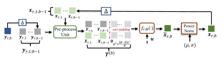
Figure 3: The signal generation process of the $b$-th block at the relay node in the full-duplex relay case. $\Delta$ denotes unit delay. The ‘Pre-process Unit’ first converts the vectors $\bm{x}_{r,j},\bm{y}_{r,j}$ to their corresponding matrices, $\bm{X}_{r,j},\bm{Y}_{r,j},j\in[1,b-1]$, and then performs zero padding to obtain $\bm{T}^{(b)}$. The variables $\mu$ and $\sigma$ are introduced in (28) for power normalization.

At the $b$-th block, the relay has access to all the past received signals, $\bm{y}_{r,1:(b-1)}$, and its own transmitted signals, $\bm{x}_{r,1:(b-1)}$. All these signals will be given as input to the relay encoding function $f_{r,\bm{\Theta}}(\cdot)$, which is a neural network parameterized by $\bm{\Theta}$. Taking all the (available) signals as input at the relay will improve the final performance, which is verified via numerical experiments in Section V. The relay transmit signal at the $b$-th block can be expressed as:

$$\bm{x}_{r,b}=f_{r,\bm{\Theta}}(\bm{y}_{r,1:(b-1)},\bm{x}_{r,1:(b-1)}).$$ (22)

We note here that the term $\bm{x}_{r,1:(b-1)}$ is equivalent to $\bm{x}_{r,2:(b-1)}$ as the relay keeps silent in the first block, yet we will adopt the former notation for consistency. The transmitted signals of the source and relay at different blocks for DeepJSCC-PF are summarized in Table. LABEL:my_schedule.

Destination Decoding. As opposed to backward decoding employed in BMC, where the destination decodes the messages in a reverse order, our DeepJSCC decoder, denoted by $g(\cdot)$, takes all the $B$ received blocks together to reconstruct the original image $\hat{\bm{S}}$, which can be expressed as:

$$\hat{\bm{S}}=g(\bm{y}_{d,1:B}).$$ (23)

IV-B2 DeepJSCC-AF

The operations at the source and the destination nodes of the DeepJSCC-AF protocol are identical to those of DeepJSCC-PF. The only difference lies in the transmitted signal at the relay, where the $b$-th block can be expressed as:

$$\bm{x}_{r,b}=\eta\bm{y}_{r,b-1},$$ (24)

where $\eta$ is the power normalization factor. Both DeepJSCC-AF and DeepJSCC-PF protocols for the full-duplex relay channel use the MSE between $\bm{S}$ and $\hat{\bm{S}}$ as the loss function as in the case of half-duplex relaying.

IV-C DNN design

Next, we investigate the intricacies of designing the DNNs at the source, relay, and destination to effectively accommodate the full-duplex relaying protocol introduced above.

IV-C1 DNNs for the encoder

Similarly to the half-duplex case, the encoding function $f_{s}(\cdot)$ at the source is realized using a standard ViT encoder, which takes the image as input and outputs a matrix $\bm{X}_{s}\in\mathbb{R}^{p^{2}\times c^{*}}$. Then, $B$ sub-matrices are obtained by partitioning along the columns expressed as:

$$\bm{X}_{s}=[\bm{X}_{s,1},\ldots,\bm{X}_{s,B}],$$ (25)

where each $\bm{X}_{s,b}\in\mathbb{R}^{p^{2}\times\frac{c^{*}}{B}}$ is converted into a complex vector of length $k/B$ for transmission.

IV-C2 DNN at the relay

The relay adopts a modified ViT encoder as its backbone. Since its input is no longer an image but a ‘knowledge matrix’ $\bm{T}\in\mathbb{R}^{p^{2}\times\frac{2c^{*}(B-1)}{B}}$ consisting of all the previous received signals as well as its own past transmitted signals, the patch partition operation is removed from the standard ViT encoder at the relay. The construction of the knowledge matrix $\bm{T}$ which corresponds to the ‘Pre-process Unit’ in Fig. 3 is described as follows: At the first block, $\bm{T}^{(1)}$ is initialized as an all-zero matrix as the relay has not yet received any signal. At the end of the $(b-1)$-th block, the relay has received $(b-1)$ blocks, $\bm{y}_{r,1:(b-1)}$, from the source and each block, $\bm{y}_{r,j}$ is a length-$k/B$ complex vector converted to a matrix $\bm{Y}_{r,j}\in\mathbb{R}^{p^{2}\times\frac{c^{*}}{B}},j\in[1,b-1]$. Similarly, each transmitted signal $\bm{x}_{r,j}$ is organized into $\bm{X}_{r,j}\in\mathbb{R}^{p^{2}\times\frac{c^{*}}{B}}$ and the updated knowledge matrix at the relay is simply:

$$\bm{T}^{(b)} =[\bm{Y}_{r,1},\ldots,\bm{Y}_{r,b-1},\bm{0}_{p^{2}\times\frac{(B-b)c^{*}}{B}},$$

$$\bm{X}_{r,1},\ldots,\bm{X}_{r,b-1},\bm{0}_{p^{2}\times\frac{(B-b)c^{*}}{B}}],$$ (26)

where $\bm{0}_{p^{2}\times\frac{(B-b)c^{*}}{B}}$ denotes an all-zero matrix with dimension $(p^{2},\frac{(B-b)c^{*}}{B})$. In the $b$-th block, the relay encoder $f_{r,\Theta}(\cdot)$ takes $\bm{T}^{(b)}$ as input and outputs $\tilde{\bm{x}}_{r,b}\in\mathbb{R}^{\frac{2k}{B}}$:

$$\tilde{\bm{x}}_{r,b}=f_{r,\Theta}(\bm{T}^{(b)}).$$ (27)

We remark that the relay starts from an all-zero knowledge matrix $\bm{T}^{(1)}$, and gradually populates it as blocks progress, and we expect the ViT encoder at the relay to acquire increasingly higher quality features about the source image to be forwarded to the destination.

Power normalization at the relay. Before transmitting $\tilde{\bm{x}}_{r,b}$ to the destination, a power normalization layer is needed to satisfy the relay power constraint. At a first glance, the same power normalization at the source can be adopted at the relay node. However, since the relay has no access to the future blocks with index $j>b$ when performing power normalization for the current block with index $b$, a new power normalization scheme is needed. To tackle this, we adopt the scheme used in the deep learning-aided feedback code design[32, 33]. During training, we record the mean $\mu$ and variance $\sigma^{2}$ of $\tilde{\bm{x}}_{r}$ of the transmitted symbols:

$$\mu =\frac{B}{2k(B-1)}\sum_{b=2}^{B}\sum_{n=1}^{2k/B}{\tilde{\bm{x}}_{r,b}[n]},$$

$$\sigma^{2}= \frac{B}{2k(B-1)}\sum_{b=2}^{B}\sum_{n=1}^{2k/B}{(\tilde{\bm{x}}_{r,b}[n]-\mu)^{2}}.$$ (28)

Note that the calculation of $\mu,\sigma$ starts from block $b=2$ since the relay keeps silent in the first block. At the inference time, the power normalization is performed in a block wise manner:

$$\tilde{\bm{x}}^{\prime}_{r,b}=\sqrt{\frac{Pr}{2}}\frac{\tilde{\bm{x}}_{r,b}-\mu}{\sigma},\quad b\in[2,B]$$ (29)

where $\sqrt{1/2}$ is introduced due to the fact that $\tilde{\bm{x}}_{r,b}$ is a real-valued vector. Finally, we convert $\tilde{\bm{x}}^{\prime}_{r,b}$ to a complex vector, $\bm{x}_{r,b}\in\mathbb{C}^{\frac{k}{B}}$, which will be forwarded to the destination. Fig. 3 illustrates the entire relay encoding process for the $b$-th block.

IV-C3 DNNs for the decoder

Finally, the decoder at the destination node, denoted as $f_{d}(\cdot)$, takes all the received signals as input to reconstruct the original image $\bm{S}$. Similarly to the processing at the relay, the received signal at the destination at the $b$-th block, $\bm{y}_{d,b}$ is converted into a matrix $\bm{Y}_{d,b}\in\mathbb{R}^{p^{2}\times\frac{c^{*}}{B}}$ and we concatenate all the $B$ matrices along the columns, $\bm{Y}_{d}=[\bm{Y}_{d,1},\ldots,\bm{Y}_{d,B}]$, which will be fed to the decoder function, $f_{d}(\cdot)$. A standard ViT decoder model introduced in Section III-A with $N_{d}$ attention blocks is utilized to parameterize $f_{d}(\cdot)$.

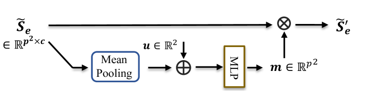
Figure 4: The neural processing at the LA model located at the ViT encoder, where $\oplus$ denotes vector concatenation, and $\otimes$ denotes token-wise multiplication.

IV-D Adaptive Transmission

As shown in Fig. 1(b), the full-duplex relay channel is determined by variables such as link qualities $c_{sr},c_{sd},c_{rd}$ and the average transmission power at the source and the relay, i.e., $P_{s}$ and $P_{r}$, respectively. If a new model is trained for each and every tuple of these variables, the memory cost for storing these models would be prohibitive. Thus, to make the DeepJSCC protocols more practical, training a single model to be adaptive to different variables is desired.

To begin with, we simplify the problem by assuming the average power at the source and the relay to be identical, i.e., $P_{s}=P_{r}=P$, where $P$ is fixed. Moreover, we set $c_{sd}$ to unity while $c_{rd}$ and $c_{sr}$ can vary within a range from $c_{min}$ to $c_{max}$.

To train the adaptive model, we first reveal the side information, denoted as $\bm{u}=[c_{sr},c_{rd}]$, to the source, relay and destination nodes. A new neural network architecture, termed as link-adaptive (LA) module at these nodes utilizes the side information to facilitate the generation of the output signal for the specific link qualities. We illustrate the LA module at the source node as an example while the processing of the LA modules at the relay (if DeepJSCC-PF is adopted) and destination are the same. As shown in Fig. 2, the LA module is located directly after the self-attention modules. Denoting the output of the self-attention module as $\widetilde{\bm{S}}_{e}\in\mathbb{R}^{p^{2}\times c}$, the LA module takes $\widetilde{\bm{S}}_{e}$ and the side information as input and learns to assign different weights $\bm{m}$ to different tokens belonging to $\widetilde{\bm{S}}_{e}$:

$$\bm{m} =\text{MLP}\left(\left[\frac{1}{c}\sum_{j=1}^{c}\widetilde{\bm{S}}_{e}[1,j],\ldots,\frac{1}{c}\sum_{j=1}^{c}\widetilde{\bm{S}}_{e}[p^{2},j],\bm{u}\right]\right),$$

$${\widetilde{\bm{S}}_{e}^{\prime}} =\bm{m}\otimes\widetilde{\bm{S}}_{e},$$ (30)

where $\bm{m}$ is of length-$p^{2}$ and $\otimes$ represents token-wise multiplication. The flowchart of the LA module is shown in Fig. 4.

In the training phase, for each batch, we randomly sample a pair of $(c_{sr},c_{rd})$ from $\mathcal{U}(c_{min},c_{max})$, and feed them to the DNNs at the source, relay and destination node, respectively. All these DNN models are jointly optimized via end-to-end training. We will show in the simulation section that with the adaptive transmission model, our scheme can achieve comparable reconstruction performance with respect to the separately trained models for each $(c_{sr},c_{rd})$ pair.

TABLE III: List of key variables

Variable	Description
$c_{sd}$	Channel quality for the source-to-destination link, set to unity by default.
$c_{sr}$	Channel quality for the source-to-relay link.
$c_{rd}$	Channel quality for the relay-to-destination link.
$P_{s}$	Average transmission power of the source node.
$P_{r}$	Average transmission power of the relay node.
$R^{*}_{hd}$	The rate achieved by the maximum of the DF and CF protocols in the half-duplex mode.
$R^{*}_{fd}$	The rate achieved by the maximum of the DF and CF protocols in the full-duplex mode.
$\alpha$	The time-division variable defined as the proportion of the relay-transmit period over the entire period.
$\gamma$	The power allocated to $\bm{x}_{s}^{(1)}$ in the half-duplex relaying, defined as $\gamma=\frac{\mathbb{E}{\|\bm{x}_{s}^{(1)}\|^{2}_{2}}}{\mathbb{E}{\|\bm{x}_{s}\|^{2}_{2}}}$.
$\beta$	The correlation between the $\bm{x}^{(2)}_{s}$ and $\bm{x}_{r}$ in the half-duplex relaying, defined as $\beta=\frac{\mathbb{E}{(\bm{x}_{r}^{\dagger}\bm{x}_{s}^{(2)}})}{\sqrt{\mathbb{E}{\|\bm{x}_{s}^{(2)}\|^{2}_{2}}\mathbb{E}{\|\bm{x}_{r}\|^{2}_{2}}}}$.
$B$	Number of blocks adopted by the full-duplex relaying.
$t$	The number of previous blocks that the relay takes as input for the full-duplex case.

V Numerical Experiments

V-A Parameter Settings and Training Details

We evaluate the effectiveness of the proposed DeepJSCC-AF and PF protocols in both half-duplex and full-duplex relay channels considering the transmission of images from the CIFAR-10 dataset, which consists of $50,000$ training and $10,000$ test RGB images with $32\times 32$ resolution.

The ViT modules are used as the backbone for the DeepJSCC models. In particular, we set the parameter $p$ for the image-to-sequence transformation module to $8$, the number of hidden neurons in the MLP layers to $c=256$, and unless otherwise mentioned, the number of transformer layers at the source, relay (if DeepJSCC-PF is adopted) and destination nodes are set to 6, 4, and 8, respectively.

In the training phase, Adam optimizer is adopted with a varying learning rate, initialized to $10^{-4}$ and reduced by a factor of $0.9$ if the validation loss does not improve in $20$ consecutive training epochs. The batch size for training is $64$ and the maximum number of epochs to train the models is set to $2\times 10^{3}$ to ensure that the reconstruction performance saturates with respect to the number of epochs. To avoid potential waste of computing resources during training, early stopping is used where the training process terminates if the validation loss does not improve over $60$ epochs.

Unless otherwise mentioned, for both half-duplex and full-duplex models, we fix a CPP of $\rho=0.25$, and hence, $c^{*}=24$. We assume that the relay lies in between the source and the destination with $c_{sr},c_{rd}\in[0,10]$ dB while $c_{sd}=0$ dB. Moreover, simplifications are made where identical average power is considered at the source and the relay, i.e., $P_{s}=P_{r}=P$ with $P$ fixed at $3$ dB.

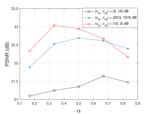
Figure 5: The PSNR performance for the half-duplex relay channel with different $\alpha$ values, $\alpha\in\{1/6,2/6,3/6,4/6,5/6\}$. The system settings are $(c_{sr},c_{rd})=(0,10)$ dB, $(c_{sr},c_{rd})=(20/3,10/3)$ dB and $(c_{sr},c_{rd})=(10,0)$ dB, respectively.

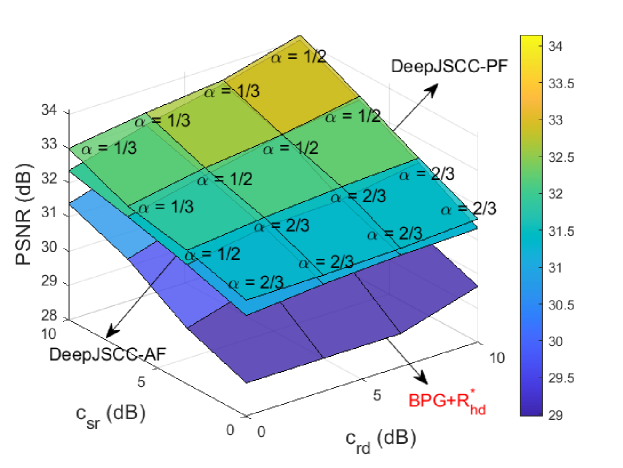
Figure 6: The PSNR performance of the proposed DeepJSCC-AF, DeepJSCC-PF and the digital baseline for the half-duplex relay channel with $c_{sr},c_{rd}\in\{0,10/3,20/3,10\}$ dB.

V-B Performance evaluation for half-duplex relay

V-B1 Overall DeepJSCC performance

We first evaluate the relative performance of the proposed DeepJSCC protocols over the state-of-the-art BPG compression algorithm delivered at a rate, $R^{*}_{hd}$, achieved by the maximum of the conventional decode-and-forward ($R_{DF}$) and compress-and-forward ($R_{CF}$) protocols [3, 4] working in a half-duplex mode. To be precise, we have:

$$R^{*}_{hd}=\max{(R_{\text{DF}},R_{\text{CF}})}.$$ (31)

The closed form expressions for $R_{\text{DF}}$ and $R_{\text{CF}}$ and their dependence on the variables $P_{s},P_{r},c_{sr},c_{rd},c_{sd}$, and the time division variable $\alpha$ is provided in the Appendix.

We first show numerically that for the DeepJSCC-PF protocol, there exists an optimal $\alpha$ for each channel condition. In this simulation, we consider three relay channel conditions, namely, (1) $(c_{sr}=0,c_{rd}=10)$ dB; (2) $(c_{sr}=20/3,c_{rd}=10/3)$ dB and (3) $(c_{sr}=10,c_{rd}=0)$ dB and for each of the scenarios, $\alpha$ is selected from a discrete set, $\{1/6,2/6,\ldots,5/6\}$. The relative performance of the three settings with respect to different $\alpha$’s is shown in Fig. 5. As can be seen, the system prefers a smaller $\alpha$ when $c_{sr}$ is relatively large, while a larger $\alpha$ is more beneficial if $c_{rd}$ becomes larger. This observation is aligned with the intuition, when the source-to-relay channel is strong, relay can receive the necessary information over a shorter time period. Note that this observation aligns with that of the conventional decode-and-forward protocol [4], where the higher achievable rate, $R_{\text{DF}}$, is obtained with small $\alpha$ when $c_{sr}$ is relatively large.

Then, we compare the performance of the proposed DeepJSCC-PF with its AF counterpart as well as the digital baseline in Fig. 6. In this simulation, we set $P=3$ dB for all the schemes. All the models with DeepJSCC-AF protocol adopt a fixed $\alpha=1/2$ while the models with DeepJSCC-PF protocol select the optimal $\alpha^{*}$ given the channel conditions, i.e., $c_{sr}$ and $c_{rd}$. Various channel conditions with both $c_{sr}$ and $c_{rd}$ chosen from $\{0,10/3,20/3,10\}$ dB are evaluated, and the PSNR performances are shown in Fig. 6. We also mark the optimal $\alpha^{*}$ on the plot for all the $16$ combinations of the DeepJSCC-PF scheme. It can be seen that both the proposed DeepJSCC-AF and DeepJSCC-PF protocols outperform the digital baseline by a large margin. Moreover, the DeepJSCC-PF outperforms the DeepJSCC-AF protocol in all the considered scenarios, which is intuitive as the DNNs at the relay should perform at least as well as linear scaling of the DeepJSCC-AF. We also notice that the DeepJSCC-PF outperforms its AF counterpart especially when the channel qualities $(c_{sr},c_{rd})$ are poor. This might due to the fact that the neural network at the relay is not only capable to extract features from the received signal over the noisy $\mathrm{S}$-$\mathrm{R}$ link but also generates robust transmit signal $\bm{x}_{r}$ to combat the noise in the $\mathrm{R}-\mathrm{D}$ link.

TABLE IV: Evaluation of the important variables, $\alpha,\gamma$ and $\beta$ for the DeepJSCC-PF protocol with a half-duplex relay and $c_{rd}=10/3$ dB, while $c_{sr}\in\{0,10/3,20/3,10\}$ dB.

$c_{sr}$ (dB)	0	10/3	20/3	10
$\alpha$	4/6	4/6	3/6	2/6
$\gamma$	0.941	0.889	0.709	0.506
$\beta$	0.828	0.819	0.787	0.568

V-B2 Evaluations of important variables

We then evaluate the important variables, namely, the time division variable $\alpha$, power variable $\gamma$ and the correlation variable $\beta$, introduced in Section III to gain more insights regarding the proposed DeepJSCC-PF protocol.

In this simulation, we adopt the same setting as in Fig. 6. Note that the optimal $\alpha^{*}$ values (among the multiplies of $1/6$) for each link condition, $c_{sr}$ and $c_{rd}$ have already been marked in Fig. 6. We then explore the relationship of the variables, $\gamma$ and $\beta$ with respect to different link qualities. Due to the page limit, we provide the results for the following combinations, namely, $(c_{sr},c_{rd})=(0,10/3)$, $(c_{sr},c_{rd})=(10/3,10/3)$, $(c_{sr},c_{rd})=(20/3,10/3)$ and $(c_{sr},c_{rd})=(10,10/3)$ dB. As introduced in Section III, the calculation of $\gamma$ and $\beta$ follows $\gamma=\frac{\mathbb{E}{\|\bm{x}_{s}^{(1)}\|^{2}_{2}}}{\mathbb{E}{\|\bm{x}_{s}\|^{2}_{2}}}$ and $\beta=\frac{\mathbb{E}{(\bm{x}_{r}^{\dagger}\bm{x}_{s}^{(2)}})}{\sqrt{\mathbb{E}{\|\bm{x}_{s}^{(2)}\|^{2}_{2}}\mathbb{E}{\|\bm{x}_{r}\|^{2}_{2}}}}$, respectively.

As can be seen in Table IV, when $c_{sr}$ improves, the $\gamma$ of the learned models with the optimal $\alpha^{*}$ decreases. This confirms the intuition that, given a better $\mathrm{S}$-$\mathrm{R}$ link, the source can save its power in the relay-receive period and consume more power in the relay-transmit period for better performance. The correlation variable $\beta$ follows the same trend. We can argue that when the $\mathrm{S}$-$\mathrm{R}$ link is weak, the source mostly relies on direct transmission, allowing the relay to transmit only in the $1/3$ of the time and uses most of its power in the relay-receive period. On the other hand, what the source transmits in the relay-transmit period is highly correlated with relay’s signal; that is, in this period, the main goal of the source is to collaborate with the relay to forward its received information. On the other hand, as the $\mathrm{S}$-$\mathrm{R}$ link quality improves, relay-receive period shortens, as the relay can quickly recovers the information from the source and uses the remaining time to forward it to the destination. We also see that the source uses increasing amount of its power in the relay-transmit period, and with a smaller $\beta$ value, which means that the source uses more of its power to transmit fresh information in this period, while also helping the relay forward its information to the destination.

TABLE V: Comparison of the original DeepJSCC-PF protocol with the modified one under the same setting with Table IV. Note that the entries on the left corresponds to the original protocol while those on the right to the modified one.

$c_{sr}$ (dB)	0	10/3	20/3	10
PSNR	31.46/31.35	32.18/32.10	32.65/32.46	33.37/32.32
$\gamma$	0.94/0.94	0.89/0.90	0.71/0.73	0.51/0.63
$\beta$	0.82/0.85	0.80/0.88	0.79/0.96	0.57/0.75

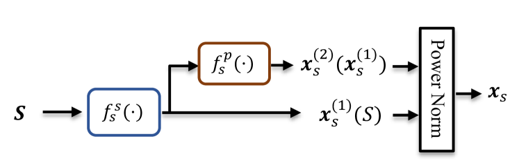
(a) DeepJSCC-PF protocol.

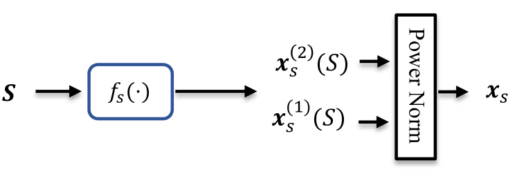
(b) Modified protocol.

Figure 7: Illustration of the source encoder for the DeepJSCC-PF protocol (a) and its modified version (b) where no new information is transmitted in the relay-transmit period.

V-B3 Transmission without new information

To better understand the source behaviour, we further consider an extreme case for the half-duplex relay mode, in which no new information is transmitted by the source node in the relay-transmit period. As shown in Fig. 7(b), we introduce the ‘systematic’ ViT encoder at the source, denoted as $f_{s}^{s}(\cdot)$ to generate $\bm{x}_{s}^{(1)}$ with dimension $\alpha^{*}k$, then $\bm{x}_{s}^{(1)}$ is fed to the ‘parity’ encoder, denoted as $f_{s}^{p}(\cdot)$, also a ViT encoder as in Fig. 2 but without the image-to-sequence transformation module to obtain the ‘parity’ signal $\bm{x}_{s}^{(2)}$ with dimension $(1-\alpha^{*})k$. Note that $\bm{x}_{s}^{(2)}$ is generated using $\bm{x}_{s}^{(1)}$, so no new information can be transmitted by the source during the relay-transmit period. $\bm{x}_{s}^{(1)}$ and $\bm{x}_{s}^{(2)}$ are then power normalized to generate the final transmitted signal. To show the effect of transmitting the new information $w_{2}$, in this experiment, we adopt the same setting with that in Table IV where the models are evaluated with varying $c_{sr}\in\{0,10/3,20/3,10\}$ dB and a fixed $c_{rd}=10/3$ dB. We further emphasize that the same $\alpha^{*}$ values are adopted to obtain the values in Table V.

We show the comparison between the original DeepJSCC-PF with the modified one in Table V. Note that we use $\alpha^{*}$ values reported in Table IV. As can be seen in the table, when the link qualities are bad, e.g., $c_{sr}=0$ and $10/3$ dB, the original DeepJSCC-PF protocol outperforms the modified one by a small margin showing that in these cases, only a small amount of new information, is transmitted in the original DeepJSCC-PF protocol. When the $c_{sr}$ improves, it can be seen that transmitting new information is essential to achieve good performance where a 1 dB PSNR gain is observed when $c_{sr}=10$ dB. It can also be seen from the table that the modified protocol always has a larger $\beta$ compared with the original one, as the source is not transmitting any new information it mainly tries to align its codeword with that of the relay for beamforming gains. The reason they cannot be aligned perfectly (unlike in the original DF scheme) is due to the noise in the $\mathrm{S}$-$\mathrm{R}$ link and the fact that the DeepJSCC-PF scheme cannot remove the noise in the received signal completely.

V-C Performance evaluation for full-duplex relaying

Next, we compare the relative performance of the DeepJSCC-AF, DeepJSCC-PF and the state-of-the-art BPG image compression algorithm delivered at a rate, denoted as $R^{*}_{fd}$, which is determined by the maximum of the achievable rates attained by the DF and CF protocols in the full-duplex case whose closed form expressions are given in the Appendix.

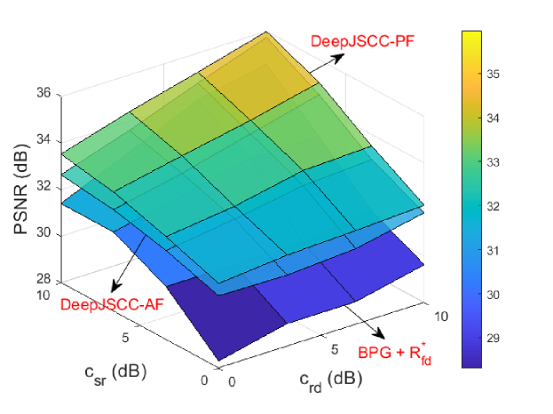
Figure 8: The PSNR performance of the proposed DeepJSCC-AF and PF protocols and the digital baseline for the full-duplex relay channel with $c_{sr},c_{rd}\in\{0,10/3,20/3,10\}$ dB.

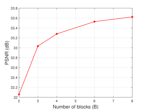
Figure 9: The PSNR performance of the proposed DeepJSCC-PF protocol for the full-duplex relay channel with different number of blocks $B=\{2,3,4,6,8\}$ under $P=3,c_{sr}=c_{rd}=5$ dB.

V-C1 DeepJSCC performance

To start with, we consider the case where $B=6$, $P=3$ dB, while $c_{sr}$ and $c_{rd}$ are chosen from the set $\{0,10/3,20/3,10\}$ dB. The relative PSNR performance for the two proposed DeepJSCC protocols as well as the digital baseline are shown in Fig. 8. Note that we set the number of blocks to a moderate number $B=6$ for both DeepJSCC-AF and PF protocols. As can be seen from the figure, both DeepJSCC-AF and PF protocols outperform the digital baseline. Compared with the results obtained with a half-duplex relay, the full-duplex relay yields a better performance, which is expected since the relay is able to communicate with the destination over the whole period. Also aligned with our expectation, DeepJSCC-PF outperforms DeepJSCC-AF, but the gap between the two diminishes as $c_{sr}$ and $c_{rd}$ improve. This is due to the fact that less noise is forwarded by DeepJSCC-AF in this case.

V-C2 Effects of different number of blocks

Intuitively, there is a trade-off between the reconstruction performance and the relay processing complexity (or, equivalently, the number of blocks). Note that when $B=1$, the scheme degrades to point-to-point transmission while for $B=2$, it degrades to a half-duplex relay since the relay keeps silent in the first block anyway. Therefore, there is a trade-off between the complexity and the performance of the scheme, which can be adjusted by choosing the $B$ value.

To characterize this trade-off, we set the number of blocks $B\in\{2,3,4,6,8\}$, $P=3$ dB, $c_{sr}=c_{rd}=5$ dB and present the achieved performances in Fig. 9. As can be seen, the reconstruction quality grows rapidly from $B=2$ to $B=6$, while it starts to saturate after $B=8$. We set $B=6$ for the simulations throughout this paper. It can also be verified in the figure that the half-duplex result matches the full-duplex case with $B=2$.

TABLE VI: Evaluation of the DeepJSCC-PF protocol for the full-duplex relay with different number of memory values $t\in\{1,2,5\}$ under $P=3,c_{sr}=c_{rd}=5$ dB and $B=6$.

Memory $t$	1	2	5	DeepJSCC-AF
PSNR (dB)	32.91	33.48	33.51	32.88
SSIM	0.968	0.972	0.972	0.967

V-C3 Relaying with memory

As illustrated in Section IV, in the conventional block Markov coding, the relay generates its transmitted signal for the $b$-th block, $\bm{x}_{r,b}$ based on $\bm{x}_{r,b-1}$ and $\bm{y}_{r,b-1}$. In the DeepJSCC-PF, we generalize the operations at the relay in the BMC scheme by introducing the ‘knowledge matrix’ $\bm{T}^{(b)}$, which includes all the information (not only the $(b-1)$-th block but also previous blocks) available so far to improve the reconstruction performance.

To outline the effectiveness of the signal from previous blocks, $j<b$, we introduce an memory variable $t\in[1,B-1]$ which determines the maximum number of previous blocks used to generate the output $\bm{x}_{r,b}$. In particular, for the $b$-th block, the ‘knowledge matrix’ $\bm{T}^{(b)}_{t}\in\mathbb{R}^{p^{2}\times\frac{2c^{*}(B-1)}{B}}$ with memory $t$ is given as

$$\bm{T}^{(b)}_{t}=\begin{cases}\begin{aligned} ,\end{aligned}&\text{if $b=B$.}\\ \begin{aligned} ,\end{aligned}&\text{if $t+1<b<B$.}\\ \begin{aligned} ,\end{aligned}&\text{otherwise.}\end{cases}$$ (32)

We present the performance of the DeepJSCC-PF with $B=6$, $t\in\{1,2,5\}$ and $(c_{sr},c_{rd},P)=(5,5,3)$ dB in Table VI. Note that the $t=B-1=5$ case is the same with the DeepJSCC-PF curve in Fig. 8. It is shown in the table that having $t=1$ as in the conventional BMC scheme is not enough leading to a PSNR gap larger than $0.5$ dB compared with the $t=5$ case. We also find that the DeepJSCC-AF protocol with a memory of one is only slightly outperformed by the DeepJSCC-PF with $t=1$ indicating the gain of the DeepJSCC-PF protocol mainly comes from larger memory values. Finally, it is observed that having $t=2$ is enough to achieve a similar reconstruction performance with that of $t=5$.

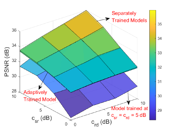
Figure 10: The PSNR comparison between the separately trained models (testing conditions are identical to the training conditions), the adaptive transmission model and the model trained at $c_{sr}=c_{rd}=5$ dB working in a full-duplex mode evaluated under $c_{sr},c_{rd}\in\{0,10/3,20/3,10\}$ dB.

V-C4 Adaptive transmission model

Following the link quality adaptive model described in Section IV-D, we optimize a single adaptive transmission model with $(c_{min},c_{max})=(0,10)$ dB. In this simulation, we focus on the DeepJSCC-PF protocol and adopt the identical setting with that in Fig. 8, i.e., $B=6,P=3$ dB. The adaptively trained model is evaluated under $c_{sr},c_{rd}\in\{0,10/3,20/3,10\}$ dB, whose overall reconstruction performance is compared with that of separately trained models in Fig. 10. Since training an adaptive transmission model is generally harder, we adopt a slightly larger patience value where the learning rate drops by $0.9$ if the validation loss does not improve in $25$ consecutive epochs ($20$ for the separately trained models).

As can be seen from the figure, only a negligible PSNR gain is obtained by training distinct models for different channel conditions, showing the effectiveness of the proposed ‘LA module’ introduced in Section IV. The model trained at a fixed channel quality $c_{sr}=c_{rd}=5$ dB achieves slightly better reconstruction performance than the adaptive transmission model when evaluated at the channel qualities it is trained at, but its performance degrades rapidly when the channel conditions change. Nevertheless, the curve obtained from the model trained at fixed $c_{sr}=c_{rd}=5$ dB illustrates that the proposed DeepJSCC-PF protocol avoids the cliff and leveling effects as its PSNR performance gracefully degrades with lower $c_{sr}$ and $c_{rd}$ values while improving with better channel qualities.

(a) Original

(b) PSNR/SSIM

(c) BPG+$R_{hd}^{*}$

(d) 29.25/0.891

(e) DeepJSCC-PF (HD)

(f) 31.61/0.9370

(g) BPG+$R_{fd}^{*}$

(h) 31.06/0.9177

(i) DeepJSCC-PF (FD)

(j) 32.73/0.9501

(k) PSNR/SSIM

(l) 27.68/0.9236

(m) 29.50/0.9579

(n) 29.29/0.9470

(o) 30.29/0.9640

(p) PSNR/SSIM

(q) 28.91/0.9374

(r) 31.58/0.9644

(s) 30.58/0.950

(t) 32.07/0.9692

Figure 11: Visualizations of the reconstructed images from the CelebA dataset obtained by the proposed DeepJSCC-PF scheme as well as the BPG compression algorithm delivered at rates $R^{*}_{hd}$ and $R^{*}_{fd}$, respectively, with half-duplex and full-duplex relays, with $\text{CPP}=0.0234$. The PSNR and SSIM results are also provided for the reconstructed images.

V-D Large Datasets

Finally, we evaluate our scheme on larger datasets and show that the learned DeepJSCC neural networks are capable to provide visually pleasing reconstructions in a large variety of network conditions. In this simulation, all the models are trained and tested with the CelebA [34] dataset with a resolution of $128\times 128$. To be precise, we consider the case where the link qualities are $(c_{sr},c_{rd},c_{sd})=(10,10,0)$ dB while the transmission power at the source and the relay are set to $P=3$ dB. The DeepJSCC-PF protocol for both the half-duplex and full-duplex scenarios is compared with the BPG image compression baseline. To be precise, the DeepJSCC-PF model for half-duplex relay is evaluated with $\alpha=3/6$ (the best $\alpha$ value from the set $\{1/6,\cdots,5/6\}$) while for the full-duplex relay, we set $B=6$ and the memory size to $t=5$. For the baseline scheme, we assume that the BPG compression output is delivered at the rates $R^{*}_{hd}$ and $R^{*}_{fd}$ for half-duplex and full-duplex cases, respectively.

It is worth mentioning that, for large datasets with high resolution, the ViT [28] model used in the previous sections is no longer feasible. The reason is that, in the ViT model, the multi-head self attention is calculated between each token and all the remaining tokens, which leads to a quadratic complexity, $\mathcal{O}((HW)^{2})$ with respect to the image size, where $H,W$ denote the height and width of the image. When the image size is large, ViT models are less effective with high complexity. To solve this, researchers have proposed more advanced solutions, e.g., the Twins transformer [35] which is adopted as the backbone of the DeepJSCC models for the CelebA dataset and we refer interested readers to [35] for more details. For the simulation, the image-to-sequence transformation parameter is set to $p=8$, which is identical to the configuration for the CIFAR-10 dataset and we have $c^{*}=36$, resulting in a CPP value of $\rho=0.0234$.

Visualizations of different CelebA images are provided in Fig. 11 obtained by different schemes. As can be seen, for both half-duplex and full-duplex relays, the proposed DeepJSCC-PF outperforms the baseline separation-based scheme. In particular, DeepJSCC-PF not only yields superior PSNR and SSIM values but also produces more visually-pleasing reconstructions.

VI Conclusion

We presented a novel DeepJSCC scheme for image transmission over a cooperative relay channel, accommodating both the half-duplex and full-duplex relay scenarios. Our work presents two distinct DeepJSCC protocols, DeepJSCC-AF and DeepJSCC-PF, tailored to these relay modes. For enhanced adaptability in the context of full-duplex relay channels, we introduced the LA module, which allows a single DeepJSCC model to flexibly adjust its encoding to varying link qualities. We provided an in-depth analysis alongside meticulously designed experiments to elucidate the rationale behind our proposed DeepJSCC frameworks, with a particular focus on the DeepJSCC-PF protocol. We demonstrated the efficacy of the proposed DeepJSCC-PF schemes through extensive numerical experiments using CIFAR-10 and CelebA datasets. Our results not only showcase impressive image reconstruction performance compared to the digital baseline, which employs the BPG compression algorithm and communicates at a rate achieved by the best of conventional DF and CF protocols, but also mitigate issues like the cliff and leveling effects in both half-duplex and full-duplex relay scenarios.

Furthermore, we highlight potential avenues for future research:

• The unified DeepJSCC-PF model for half-duplex relay channels: we envision the development of a unified DeepJSCC-PF model designed specifically for half-duplex relay channels. This entails establishing a systematic method for determining the optimal time-division variable $\alpha^{*}$ for given link quality parameters $(c_{sr},c_{rd},c_{sd})$. Once determined, this $\alpha^{*}$ can be incorporated into the framework alongside the link quality values, allowing us to achieve reconstruction performance on par with separately trained DeepJSCC-PF models for fixed $(c_{sr},c_{rd},c_{sd})$ and $\alpha^{*}$ values.

• Extension to challenging fading channels: We aim to extend the applicability of our proposed DeepJSCC scheme to more complex fading channels, including MIMO and OFDM channels. Exploring these challenging environments could further expand the scope and impact of DeepJSCC.

Appendix A The BPG Baseline

This section details the BPG baseline for both half-duplex and full-duplex relay channels. For a given bandwidth ratio, $\rho$, the number of real channel uses is $2M\rho$, where $M$ is the number of pixels of the input image. The number of available bits for each image is $2M\rho R^{*}$, where the exact formula of $R^{*}$ for both half-duplex and full-duplex relay channel, denoted by $R^{*}_{hd}$ and $R^{*}_{fd}$, respectively, are given as follows.

A-A $R^{*}_{hd}$ for the half-duplex relay

The channel capacity $R_{DF}$ of the half-duplex relay channel has been derived in [4], giving

$$R_{DF}=\max_{0\leq\beta\leq 1}\min\{C_{1}(\beta),C_{2}(\beta)\},$$ (33)

where

$$C_{1}(\beta)=\frac{\alpha}{2} \log(1+c_{sr}^{2}P_{s}^{(1)})$$

$$+\frac{1-\alpha}{2} \log(1+(1-\beta)c_{sd}^{2}P_{s}^{(2)}),$$ (34)

$$C_{2}(\beta)=\frac{\alpha}{2} \log(1+c_{sd}^{2}P_{s}^{(1)})$$

$$+\frac{1-\alpha}{2} \log(1+c_{sd}^{2}P_{s}^{(2)}+c_{rd}^{2}P_{r}$$

$$+ 2c_{sd}c_{rd}\sqrt{\beta P_{s}^{(2)}P_{r}});$$ (35)

$\alpha\in(0,1)$ is the time-division variable; $\beta$ denotes the correlation between $\bm{x}_{r}$ and $\bm{x}_{s}^{(2)}$; $P_{s}^{(1)}$ and $P_{s}^{(2)}$ represent the average transmit power at the relay-receive and relay-transmit period, respectively (see (17)). Then, $R_{CF}$ can be written as

$$R_{CF}=\frac{\alpha}{2} \log(1+c_{sd}^{2}P_{s}^{(1)}+\frac{c_{sr}^{2}P_{s}^{(1)}}{1+\sigma^{2}_{w}})$$

$$+\frac{1-\alpha}{2} \log(1+P_{s}^{(2)}),$$ (36)

where

$$\sigma^{2}_{w}=\frac{c_{sr}^{2}P_{s}^{(1)}+c_{sd}^{2}P_{s}^{(1)}+1}{(c_{sd}^{2}P_{s}^{(1)}+1)((1+\frac{c_{rd}^{2}P_{r}}{1+c_{sd}^{2}P_{s}^{(2)}})^{1/\alpha-1}-1)}.$$ (37)

Combining (33) and (36), we need to figure out an optimal combination of the variables $(\alpha,P_{s}^{(1)},P_{s}^{(2)},\beta)$ given the link qualities $(c_{sr},c_{rd})$ ($c_{sd}$ is fixed to be unity in our setting) and the $P_{s},P_{r}$ values. Notice from (17) that $P_{s}^{(1)}$ and $P_{s}^{(2)}$ are determined by given fixed $P_{s}$, we carry out a brute-force searching approach given that $\alpha,\beta,\gamma\in(0,1)$. Specifically, we calculate $R_{DF}$ and $R_{CF}$ by emulating $\alpha,\beta,\gamma$ values each with a unit interval equals to $10^{-3}$ and choose the one yielding the largest $R^{*}_{hd}$ from $\approx 10^{9}$ possible combinations.

A-B $R^{*}_{fd}$ for the full-duplex relay

The derivation of $R^{*}_{fd}$ follows the same procedure as the half-duplex case. For the full-duplex, $R_{DF}$ and $R_{CF}$ are given by

$$R_{DF}=\frac{1}{2} \log(1+(1-\beta)c_{sr}^{2}P_{s})$$

$$+\frac{1}{2} \log(1+c_{sd}^{2}P_{s}+c_{rd}^{2}P_{r}+2c_{sd}c_{rd}\sqrt{\beta P_{s}P_{r}})$$ (38)

and

$$R_{CF}=\frac{1}{2} \log(1+c_{sd}^{2}P_{s}+\frac{c_{sr}^{2}P_{s}}{1+\frac{c_{sd}^{2}P_{s}+c_{sr}^{2}P_{s}+1}{c_{rd}^{2}P_{r}}}).$$ (39)

The maximum $R_{DF}$ is calculated from $10^{3}$ different $\beta$ values with a unit interval equals to $10^{-3}$.

After obtaining $R^{*}$ for both half-duplex and full-duplex relay, we will use BPG compression algorithm to compress each image to $2MR^{*}\rho$ and the average PSNR can be obtained. We note that similar with the analysis in [4], for both half-duplex and full-duplex cases, with large $c_{sr}$, $R^{*}$ is achieved by DF protocol while when $c_{sr}$ drops, $R_{CF}$ is better and $R^{*}$ is obtained by the CF protocol.

References

- [1] C. Bian, Y. Shao, H. Wu, and D. Gündüz, “Deep joint source-channel coding over cooperative relay networks,” in IEEE International Conference on Machine Learning for Communication and Networking, 2024.
- [2] A. Sendonaris, E. Erkip, and B. Aazhang, “User cooperation diversity. Part I. system description,” IEEE Transactions on Communications, vol. 51, no. 11, pp. 1927–1938, 2003.
- [3] T. Cover and A.E. Gamal, “Capacity theorems for the relay channel,” IEEE Transactions on Information Theory, vol. 25, no. 5, pp. 572–584, 1979.
- [4] A. Host-Madsen and J. Zhang, “Capacity bounds and power allocation for wireless relay channels,” IEEE Transactions on Information Theory, vol. 51, no. 6, pp. 2020–2040, 2005.
- [5] G. Kramer, M. Gastpar, and P. Gupta, “Cooperative strategies and capacity theorems for relay networks,” IEEE Transactions on Information Theory, vol. 51, no. 9, pp. 3037–3063, 2005.
- [6] A.E. Gamal and Y.-H. Kim, Network Information Theory, Cambridge University Press, 2011.
- [7] M. Uppal, Z. Liu, V. Stankovic, and Z. Xiong, “Compress-forward coding with BPSK modulation for the half-duplex Gaussian relay channel,” IEEE Transactions on Signal Processing, vol. 57, no. 11, pp. 4467–4481, 2009.
- [8] Z. Liu, S. Cheng, A.D. Liveris, and Z. Xiong, “Slepian-wolf coded nested lattice quantization for wyner-ziv coding: High-rate performance analysis and code design,” IEEE Transactions on Information Theory, vol. 52, no. 10, pp. 4358–4379, 2006.
- [9] I. Estella Aguerri and D. Gündüz, “Capacity of a class of state-dependent orthogonal relay channels,” IEEE Transactions on Information Theory, vol. 62, no. 3, pp. 1280–1295, 2016.
- [10] A. Wyner and J. Ziv, “The rate-distortion function for source coding with side information at the decoder,” IEEE Transactions on Information Theory, vol. 22, no. 1, pp. 1–10, 1976.
- [11] D. Gündüz, E. Erkip, A. Goldsmith, and H.-V. Poor, “Reliable joint source-channel cooperative transmission over relay networks,” IEEE Transactions on Information Theory, vol. 59, no. 4, pp. 2442–2458, 2013.
- [12] H.-Y. Shutoy, D. Gündüz, E. Erkip, and Y. Wang, “Cooperative source and channel coding for wireless multimedia communications,” IEEE Journal of Selected Topics in Signal Processing, pp. 295–307, 2007.
- [13] H. Kim, R. Annavajjala, P.-C. Cosman, and L.-B. Milstein, “Source-channel rate optimization for progressive image transmission over block fading relay channels,” IEEE Transactions on Communications, vol. 58, no. 6, pp. 1631–1642, 2010.
- [14] E. Bourtsoulatze, D. B. Kurka, and D. Gündüz, “Deep joint source-channel coding for wireless image transmission,” IEEE Transactions on Cognitive Communications and Networking, 2019.
- [15] J. Xu, T.-Y. Tung, B. Ai, W. Chen, Y. Sun, and D. Gündüz, “Deep joint source-channel coding for semantic communications,” IEEE Communications Magazine, vol. 61, no. 11, pp. 42–48, 2023.
- [16] M. Yang, C. Bian, and H.-S. Kim, “OFDM-guided deep joint source channel coding for wireless multipath fading channels,” IEEE Trans. on Cogn. Comm. and Networking, vol. 8, no. 2, pp. 584–599, 2022.
- [17] J. Xu, B. Ai, W. Chen, A. Yang, P. Sun, and M. Rodrigues, “Wireless image transmission using deep source channel coding with attention modules,” IEEE Trans. on Circuits and Systems for Video Tech., 2021.
- [18] T.-Y. Tung and D. Gündüz, “Deepwive: Deep-learning-aided wireless video transmission,” IEEE Journal on Selected Areas in Communications, vol. 40, no. 9, pp. 2570–2583, 2022.
- [19] S. Wang, J. Dai, Z. Liang, K. Niu, Z. Si, C. Dong, X. Qin, and P. Zhang, “Wireless deep video semantic transmission,” IEEE Journal on Selected Areas in Communications, vol. 41, no. 1, pp. 214–229, 2023.
- [20] T. Han, Q. Yang, Z. Shi, S. He, and Z. Zhang, “Semantic-preserved communication system for highly efficient speech transmission,” IEEE Journal on Selected Areas in Communications, vol. 41, no. 1, pp. 245–259, 2023.
- [21] C. Bian, Y. Shao, and D. Gündüz, “Wireless point cloud transmission,” arXiv preprint arXiv:2306.08730, 2023.
- [22] S. F. Yilmaz, C. Karamanli, and D. Gündüz, “Distributed deep joint source-channel coding over a multiple access channel,” in IEEE International Conference on Communications, 2023.
- [23] T. Wu, Z. Chen, M. Tao, B. Xia, and W. Zhang, “Fusion-based multi-user semantic communications for wireless image transmission over degraded broadcast channels,” arXiv preprint arXiv:2305.09165, 2023.
- [24] Y. Yin, L. Huang, Q. Li, B. Tang, A. Pandharipande, and X. Ge, “Semantic communication on multi-hop concatenated relay networks,” in 2023 IEEE/CIC International Conference on Communications in China (ICCC), 2023, pp. 1–6.
- [25] W. An, Z. Bao, H. Liang, C. Dong, and X. Xu, “A relay system for semantic image transmission based on shared feature extraction and hyperprior entropy compression,” IEEE Internet of Things Journal, pp. 1–1, 2024.
- [26] C. Bian, Y. Shao, and D. Gündüz, “A hybrid joint source-channel coding scheme for mobile multi-hop networks,” in IEEE International Conference on Communications, 2024.
- [27] B. Tang, L. Huang, Q. Li, A. Pandharipande, and X. Ge, “Cooperative semantic communication with on-demand semantic forwarding,” IEEE Open Journal of the Communications Society, vol. 5, pp. 349–363, 2024.
- [28] A. Dosovitskiy, L. Beyer, A. Kolesnikov, D. Weissenborn, X. Zhai, T. Unterthiner, M. Dehghani, M. Minderer, G. Heigold, S. Gelly, J. Uszkoreit, and N. Houlsby, “An image is worth 16x16 words: Transformers for image recognition at scale,” in International Conference on Learning Representations, 2021.
- [29] N. S. Ferdinand, M. Nokleby, and B. Aazhang, “Low-density lattice codes for full-duplex relay channels,” IEEE Transactions on Wireless Communications, vol. 14, no. 4, pp. 2309–2321, 2015.
- [30] A. Vaswani, N. Shazeer, N. Parmar, J. Uszkoreit, L. Jones, A. N. Gomez, L. Kaiser, and I. Polosukhin, “Attention is all you need,” in NIPS, 2017.
- [31] C. Bian, Y. Shao, and D. Gündüz, “DeepJSCC-1++: Robust and bandwidth-adaptive wireless image transmission,” in 2023 IEEE Global Communications Conference, 2023, pp. 3148–3154.
- [32] H. Kim, Y. Jiang, S. Kannan, S. Oh, and P. Viswanath, “Deepcode: Feedback codes via deep learning,” in Advances in Neural Information Processing Systems, 2018.
- [33] E. Ozfatura, Y. Shao, A. G. Perotti, B. M. Popović, and D. Gündüz, “All you need is feedback: Communication with block attention feedback codes,” IEEE Journal on Selected Areas in Information Theory, vol. 3, no. 3, pp. 587–602, 2022.
- [34] Z. Liu, P. Luo, X. Wang, and X. Tang, “Deep learning face attributes in the wild,” in Proceedings of International Conference on Computer Vision (ICCV), December 2015.
- [35] X. Chu, Z. Tian, Y. Wang, B. Zhang, H. Ren, X. Wei, H. Xia, and C. Shen, “Twins: Revisiting the design of spatial attention in vision transformers,” in Advances in Neural Information Processing Systems, 2021, vol. 34, pp. 9355–9366.