Social Optima of a Linear Quadratic
Collective Choice Model under Congestion

Abstract

This paper investigates the social optimum for a dynamic linear quadratic collective choice problem where a group of agents choose among multiple alternatives or destinations. The agents’ common objective is to minimize the average cost of the entire population. A naive approach to finding a social optimum for this problem involves solving a number of linear quadratic regulator (LQR) problems that increases exponentially with the population size. By exploiting the problem’s symmetries, we first show that one can equivalently solve a number of LQR problems equal to the number of destinations, followed by an optimal transport problem parameterized by the fraction of agents choosing each destination. Then, we further reduce the complexity of the solution search by defining an appropriate system of limiting equations, whose solution is used to obtain a strategy shown to be asymptotically optimal as the number of agents becomes large. The model includes a congestion effect captured by a negative quadratic term in the social cost function, which may cause agents to escape to infinity in finite time. Hence, we identify sufficient conditions, independent of the population size, for the existence of the social optimum. Lastly, we investigate the behavior of the model through numerical simulations in different scenarios.

Dynamic Discrete Choice Models, Optimal Control, Social Optimization, Optimal Transport.

1 Introduction

Networked systems consist of highly interdependent dynamic components or agents that interact with each other to achieve a given individual or collective purpose. These systems hold a significant importance in contemporary society, with applications spanning numerous domains including power distribution, transportation, epidemiological modeling, and analyzing social networks. Social optimization refers to the analysis of networked systems where agents aim to optimize a collective outcome, i.e., find a social optimum. As the number of agents and the complexity of their interactions grow, identifying a social optimum becomes increasingly complex. To address this challenge, various techniques are employed.

A first approach consists in using the model’s properties, .e.g., its linear quadratic (LQ) structure and symmetries, to derive an explicit analytical solution. Using this approach, Arabneydi et al. [1] derive an explicit solution for a discrete-time LQ team optimization model under full and partial information structures, and Huang et al. [2] identify the solution of a social optimization problem with controlled diffusions. Another frequently used method consists in using the person-by-person (PbP) optimality principle, reframing the search for a social optimum as a non-cooperative game [3]. Concretely, one solves the social optimization problem as a sequential optimization problem, reducing it to a single-agent problem against a given population behavior. In general, PbP optimality is only a necessary condition for social optimality. Nevertheless, under specific conditions such as static games with convex costs and specific information structures, both solutions coincide [4, Theorem 18.2].

Another important framework for the approximate analysis of large interacting dynamic multi-agent systems is the theory of Mean Field Games (MFG) [5, 6]. It assumes that inter-agent couplings vanish asymptotically with the population size, so that, in the limit, unilateral deviation by any agent does not affect the global population behavior. The MFG and PbP approaches can be combined to address social optimization problems. This is done in [7, 8, 9], where the authors derive suboptimal strategies converging to the social optimum as the population size increases. Nonetheless, this approach requires certain restrictive technical assumptions, as for PbP optimality.

This article focuses on an LQ social optimization model, with a particular focus on population transportation. For this application, modeling congestion is a critical factor to consider, often resulting in a system of partial differential equations, which hinders the analytical tractability of the solution [5, 10, 11].

In this paper, we address congestion by introducing in the agents’ cost functions a negative quadratic term that decreases with the agents’ relative spacing, thus preserving the model’s LQ structure. An advantage of LQ models is their computational tractability, which makes them suitable for real-time control and optimization. Nonetheless, the change in cost structure invalidates the conditions for PbP optimality used in [8]. Instead, we start from a finite population and exploit the model’s symmetries and LQ structure as in [2] to derive the social optimum, as well as a more efficiently computable suboptimal solution approximating the social optimum as the population size increases.

Therefore, we consider a group of agents with continuous linear dynamics, initially spread in the Euclidean space $\mathbb{R}^{n}$. By the time horizon $T$, individual agents must have moved toward one of the alternatives within a set of destination points. This is to be achieved while minimizing an overall joint quadratic cost. When we fix the fraction of agents going to each destination, we show how to compute the optimal controls and individual agent choices by solving a number of LQR problems equal to the number of destinations followed an optimal transport (OT) problem parameterized by these fractions of agents. Finally, considering the limiting system of optimality equations as the number of agents grows, we establish the convexity of the cost with respect to the vector of destination-bound agent fractions. This leads to an efficient optimization method for the infinite population, as well as a policy for the finite agent system that is shown to be asymptotically optimal as the number of agents becomes large.

The rest of the paper is organized as follows. In Section 2, we present the general formulation of our model. In Section 3, we first establish the agents’ optimal trajectories under an arbitrarily fixed agent-to-destination choices rule. Then, we provide an algorithm to identify a solution for our proposed model. In Section 3.3, we provide an upper bound on the time horizon $T$ that guarantees the existence of a solution, independently of the population size. In Sections 4 and 5.1, we provide a limiting system of equations whose solution can be used to approximate the social optimum for a large population. In Section 5.2, we provide an algorithm to compute the latter solution. Section 6 illustrates the results in simulations and Section 7 concludes the paper. In Table 1, we collect some of the notations used throughout the paper.

Table 1: Notation table

$n$	Dimension of an agent’s state vector
$N$	Population size
$D$	Number of destinations
$\otimes$	Kronecker product
$|.|$	Set cardinality operator
$\llbracket m\rrbracket$	The set $\{1,\ldots,m\}$, for $m$ a positive integer
$\Gamma^{N}$	A vector or matrix that depends on the population size $N$
$\Gamma^{(N)}$	Block diagonal matrix with $N$ repeated blocks $\Gamma$, i.e., $I_{N}\otimes\Gamma$
$1_{N}$	All-ones column vector of size $N$
$1_{NN}$	All-ones matrix of size $N\times N$
$0_{n}$	All-zeros column vector of size $n$
$0_{nn}$	All-zeros matrix of size $n\times n$
$|y|_{2}$	The Euclidean norm $\sqrt{y^{T}y}$ for a vector $y$
$[y]_{R}^{2}$	The quadratic product $y^{T}Ry$, for a given symmetric matrix $R$ and vector $y$
$\text{col}(.)$	Operator stacking its vector arguments into a column vector
$\Omega^{N}$	$\begin{aligned} &=\Bigg{\{}P^{N}=\text{col}\left(P_{1}^{N},\ldots,P_{D}^{N}\right)\in\mathbb{R}^{D}\Big{|}\exists N_{1},\ldots,N_{D}\in\mathbb{N}\\ &\sum_{j=1}^{D}N_{j}=N,\text{and }P_{j}^{N}=\frac{N_{j}}{N},\text{ for }j\in\llbracket D\rrbracket\Bigg{\}}\end{aligned}$
$\Omega$	$\begin{aligned} =\Big{\{}&P=\text{col}(P_{1},\ldots,P_{D})\in\mathbb{R}^{D}\Big{|}\sum_{j=1}^{D}P_{j}=1\\ &\text{ and }P_{j}\geq 0,\text{ for }j\in\llbracket D\rrbracket\Big{\}}\end{aligned}$

2 Problem Formulation

We consider a dynamic cooperative game involving $N\geq 2$ agents, initially randomly distributed identically and independently over a subset $E$ of the Euclidean space $\mathbb{R}^{n}$ according to a distribution $\mathcal{P}_{0}$, whose support is included in $E$. Before a given time horizon $T$, these agents should reach the neighborhood of one of $D$ possible destinations, denoted $d_{i}\in\mathbb{R}^{n}$, for $1\leq i\leq D$. More precisely, the agents cooperate to minimize a common social cost $J^{N}_{\text{soc}}$, i.e., to solve

$$\qquad\min_{\lambda^{N}\in\llbracket D\rrbracket^{N}}\inf\limits_{U(.)}J^{N}_{\text{soc}}(\lambda^{N},U):=\frac{1}{N}\sum\limits_{i=1}^{N}J_{i,\lambda_{i}}(u_{i},\bar{x}^{N}),$$ (1)

$$s.t.\quad\frac{d}{dt}x_{i}(t)=Ax_{i}+Bu_{i}(t),\;\;x_{i}(0)=x_{i}^{0},\;\;i\in\llbracket N\rrbracket,$$

with $x_{i}(t)\in\mathbb{R}^{n}$ the state vector of agent $i$, $u_{i}(t)\in\mathbb{R}^{m}$ its control vector, $\lambda_{i}\in\llbracket D\rrbracket$ the index of its final destination choice, $\lambda^{N}=(\lambda_{1},\ldots,\lambda_{N})$ the destination choices for the $N$ agents, and $\bar{x}^{N}(t)=\frac{1}{N}\sum_{i=1}^{N}x_{i}(t)$ the empirical population mean state. We denote $U(t)=\text{col}(u_{1}(t),\ldots,u_{N}(t))\in\mathbb{R}^{Nm}$. The individual costs in (1) are

$$J_{i,\lambda_{i}}(u_{i},\bar{x}^{N})=\int_{0}^{T}\frac{1}{2}\Big{(}-[x_{i}-\bar{x}^{N}]_{R_{x}}^{2}+[x_{i}-d_{\lambda_{i}}]^{2}_{R_{d}}$$

$$+[u_{i}]^{2}_{R_{u}}\Big{)}dt+\frac{1}{2}[x_{i}(T)-d_{\lambda_{i}}]^{2}_{M}.$$ (2)

The matrices $R_{u}$ and $M$ are symmetric positive definite, while the matrices $R_{d},R_{x}$ are symmetric positive semidefinite. The first term in the running cost in (2) is negative and captures a congestion avoidance effect. Indeed, since we have

$$\sum_{i=1}^{N}[x_{i}-\bar{x}^{N}]_{R_{x}}^{2}=\frac{1}{2N}\sum_{i=1}^{N}\sum_{j=1}^{N}[x_{i}-x_{j}]_{R_{x}}^{2},$$

avoiding the population mean trajectory is equivalent to maximizing squared interdistances between agents. The second term in the running cost increases whenever the distance between the $i^{th}$ agent position $x_{i}$ and its chosen destination $d_{\lambda_{i}}$ increases, representing a stress effect felt by individuals as long as they remain far from their destination. Overall, we aim to identify the optimal destination choices $\lambda^{N}$ and control strategies $U$ for the agents to collectively minimize (1). Note that since the running cost may be negative, agents may escape to infinity in finite time. Therefore, in our analysis we provide in Section 3.3 a sufficient condition for the existence of an optimal solution over the interval $[0,T]$.

3 Solving the Problem
for a Population of Finite Size

In this section, we provide a solution to the problem formulated in Section 2. The problem (1) involves a minimization over both the destination choices $\lambda^{N}$ and the vector of control strategies $U$. Our approach consists in first addressing the optimization over $U$, while fixing $\lambda^{N}$. Then, we fix only the fraction of agents choosing each of the destinations $P^{N}$ and find the corresponding vector of optimal individual destination choices $\lambda^{N}$. This step-wise approach enables us to identify the optimal social cost for all possible fixed vectors of agent fractions over destinations. At that stage, the identification of the optimal $\lambda^{N}$ and $U$ becomes simply a parameter optimization problem over all feasible vectors of agent fractions over destinations.

3.1 Agent Control Strategies with Given Agent-to-Destination Choices

We assume for now that the agents’ final destinations $\lambda^{N}$ are fixed and known.

We let $d_{\lambda^{N}}=\text{col}(d_{\lambda_{1}},\ldots,d_{\lambda_{N}})$, and

$$Q^{N}\coloneqq I_{N}\otimes(R_{d}-R_{x})+\frac{1}{N}1_{NN}\otimes R_{x}.$$ (3)

The following lemma, proved in Appendix A.1, expresses the social cost (1) as a function of the global state $X=\text{col}(x_{1},\ldots,x_{N})\in\mathbb{R}^{Nn}$, which satisfies

$$\frac{d}{dt}X=A^{(N)}X+B^{(N)}U.$$

Lemma 1

The social cost (1) can be expressed as follows

$$J^{N}_{\text{soc}}(\lambda^{N},U)=$$ (4)

$$\int_{0}^{T}\frac{1}{2N}\Big{\{}[X]^{2}_{Q^{N}}-2d_{\lambda^{N}}^{T}R_{d}^{(N)}X+[d_{\lambda^{N}}]^{2}_{R_{d}^{(N)}}+[U]^{2}_{R_{u}^{(N)}}\Big{\}}dt$$

$$+\frac{1}{2N}[X(T)-d_{\lambda^{N}}]^{2}_{M^{(N)}}.$$

To find a control strategy $U^{*}$ minimizing (4), we consider the quadratic value function

$$V^{N}(t,\lambda^{N})=\frac{1}{2N}X^{T}(t)\varphi^{N}(t)X(t)+\frac{1}{N}\Psi^{N}(t)^{T}X(t)+\chi^{N}(t),$$ (5)

with $\varphi^{N}(t)\in\mathbb{R}^{Nn\times Nn}$, $\chi^{N}(t)\in\mathbb{R}$, and

$$\Psi^{N}(t)=\text{col}(\Psi^{N}_{1}(t),\ldots,\Psi^{N}_{N}(t))\in\mathbb{R}^{Nn},$$ (6)

where $\Psi^{N}_{i}(t)\in\mathbb{R}^{n}$ for all $i\in\llbracket N\rrbracket$.

Let $S=BR_{u}^{-1}B^{T}$. Using dynamic programming, we find that the time-varying coefficients $\varphi^{N}(t)$, $\Psi^{N}(t)$, and $\chi^{N}(t)$ should satisfy the following differential equations

$$\frac{d}{dt}\varphi^{N} =(\varphi^{N})^{T}S^{(N)}\varphi^{N}-\varphi^{N}A^{(N)}-(A^{(N)})^{T}\varphi^{N}-Q^{N},$$ (7)

$$\frac{d}{dt}\Psi^{N} =\left(\varphi^{N}S^{(N)}-{A^{(N)}}^{T}\right)\Psi^{N}+R_{d}^{(N)}d_{\lambda^{N}},$$ (8)

$$\frac{d}{dt}\chi^{N} =\frac{1}{2N}\left([\Psi^{N}]^{2}_{S^{(N)}}-[d_{\lambda^{N}}]^{2}_{R_{d}^{(N)}}\right),$$ (9)

with the terminal conditions

$$\varphi^{N}(T) =M^{(N)},\;\Psi^{N}(T)=-M^{(N)}d_{\lambda^{N}},$$ (10)

$$\chi^{N}(T) =\frac{1}{2N}[d_{\lambda^{N}}]^{2}_{M^{(N)}}.$$ (11)

The optimal control $U^{*}$ is

$$U^{*}(t)=-(R_{u}^{(N)})^{-1}(B^{(N)})^{T}\left(\varphi^{N}(t)X(t)+\Psi^{N}(t)\right).$$ (12)

We note that $\Psi^{N}$ and $\chi^{N}$ are both solutions over $[0,T]$ of linear differential equations, which depend on $\varphi^{N}$. Hence, if a solution exists for the backward Riccati equation (7) over [0,T], then, both $\Psi^{N}$ and $\chi^{N}$ are well defined. However, the matrix $Q^{N}$ is not necessarily positive semidefinite. Therefore, the Riccati equation (7) may exhibit a finite escape time. First, from [12, Theorem 5.3], we have the following lemma.

Lemma 2

The optimal cost $\inf\limits_{U(.)}J^{N}_{\text{soc}}(\lambda^{N},U)$ is finite for any $\lambda^{N}\in\llbracket D\rrbracket^{N}$ if and only if the Riccati equation (7) has a solution defined over $t\in[0,T]$.

In Section 3.3, we shall identify sufficient conditions, independent of the population size $N$, that guarantee the existence of a finite solution for (7) over [0,T]. For the rest of this section, we assume that such conditions are met. Then, we have the following result, proved in Appendix A.2.

Lemma 3

The solution $\varphi^{N}$ to the Riccati equation (7) can be decomposed as

$$\varphi^{N}(t)=I_{N}\otimes\varphi^{N}_{1}(t)+\frac{1}{N}(1_{NN}-I_{N})\otimes\varphi^{N}_{2}(t),$$ (13)

where the diagonal and off-diagonal components $\varphi^{N}_{1}(t)\in\mathbb{R}^{n\times n}$ and $\varphi^{N}_{2}(t)\in\mathbb{R}^{n\times n}$ satisfy the equations

$$\frac{d}{dt}\varphi^{N}_{1} =[\varphi^{N}_{1}]^{2}_{S}+\frac{N-1}{N^{2}}[\varphi^{N}_{2}]^{2}_{S}-\varphi^{N}_{1}A-A^{T}\varphi^{N}_{1}$$

$$\;\;-R_{d}+\frac{N-1}{N}R_{x},\quad\varphi^{N}_{1}(T)=M,$$ (14)

$$\frac{d}{dt}\varphi^{N}_{2} =(\varphi^{N}_{1})^{T}S\varphi^{N}_{2}+(\varphi^{N}_{2})^{T}S\varphi^{N}_{1}+\frac{N-2}{N}[\varphi^{N}_{2}]^{2}_{S}$$

$$\;\;-\varphi^{N}_{2}A-A^{T}\varphi^{N}_{2}-R_{x},\quad\varphi^{N}_{2}(T)=0_{nn}.$$ (15)

For any given $j\in\llbracket D\rrbracket$, we denote by $N_{j}$ the number of agents whose final target is $d_{j}$ and by $P_{j}^{N}\coloneqq\frac{N_{j}}{N}$ the fraction of agents selecting destination $j$. Note that $P_{D}^{N}=1-\sum\limits_{j=1}^{D-1}P_{j}^{N}$ necessarily. We also define $P^{N}=\text{col}(P_{1}^{N},\ldots,P_{D}^{N})\in\Omega^{N}$, with $\Omega^{N}$ defined in Table 1. In the next lemma, proved in Appendix A.3, we show that if two agents choose the same destination, then their corresponding components of the solution $\Psi^{N}$ of (8) are identical.

Lemma 4

Define $\psi^{N}_{j}(t,P^{N})\in\mathbb{R}^{n}$, $j\in\llbracket D\rrbracket$, as the solutions to the following system of equations

$$\frac{d}{dt} \psi^{N}_{j}(t,P^{N})=\left(\varphi^{N}_{1}S-A^{T}-\frac{1}{N}\varphi^{N}_{2}S\right)\psi^{N}_{j}+R_{d}d_{j}$$ (16)

$$\;\;+\varphi^{N}_{2}S\left(\sum\limits_{k=1}^{D}P_{k}^{N}\psi^{N}_{k}\right),\quad\psi^{N}_{j}(T,P^{N})=-Md_{j}.$$

Then, recalling (6), we have $\Psi^{N}_{i}\equiv\psi^{N}_{\lambda_{i}}$ for $i\in\llbracket N\rrbracket$.

Next, we identify an analytical form for the solution of (16). The proof of this result is given in Appendix A.4.

Lemma 5

For any $j\in\llbracket D\rrbracket$, the function $\psi^{N}_{j}(t,P^{N})$ is affine with respect to $P^{N}$ and satisfies the following relation

$$\psi^{N}_{j}(t,P^{N})=\left(\sum_{k}=1^{D-1}P^{N}_{k}\alpha^{N}_{k}(t)\right)-\beta^{N}_{j}(t),$$ (17)

where $\alpha^{N}_{k}(t)\in\mathbb{R}^{n}$ and $\beta^{N}_{j}(t)\in\mathbb{R}^{n}$, are solutions of

$$\frac{d}{dt}\alpha^{N}_{k} =\left(\varphi^{N}_{1}S-A^{T}+\frac{N-1}{N}\varphi^{N}_{2}S\right)\alpha^{N}_{k}-\varphi^{N}_{2}S(\beta^{N}_{k}-\beta^{N}_{D})$$

$$\;\;\alpha_{k}^{N}(T)=0_{n},\;\;\forall k\in\llbracket D-1\rrbracket,$$ (18)

$$\frac{d}{dt}\beta^{N}_{j} =\left(\varphi^{N}_{1}S-A^{T}-\frac{1}{N}\varphi^{N}_{2}S\right)\beta^{N}_{j}+\varphi^{N}_{2}S\beta^{N}_{D}-R_{d}d_{j},$$

$$\;\;\beta^{N}_{j}(T)=Md_{j},\;\;\forall j\in\llbracket D\rrbracket.$$ (19)

In the following, we define

$$\begin{split}&\alpha^{N}=\begin{bmatrix}\alpha_{1}^{N}&\ldots&\alpha_{D-1}^{N}&0_{n}\end{bmatrix}\in\mathbb{R}^{n\times D},\\ &\beta^{N}=\begin{bmatrix}\beta_{1}^{N}&\ldots&\beta_{D}^{N}\end{bmatrix}\in\mathbb{R}^{n\times D}.\end{split}$$ (20)

Finally, in the next lemma, proved in Appendix A.5, we establish the form of the solution of (9).

Lemma 6

The solution $\chi^{N}(t,P^{N})$ of (9) is a quadratic form of $P^{N}$ and we have that

$$\frac{d}{dt}\chi^{N}=(P^{N})^{T}W^{N}P^{N}+\frac{1}{2}\sum_{j=1}^{D}P_{j}^{N}\left([\beta_{j}^{N}]^{2}_{S}-[d_{j}]^{2}_{R_{d}}\right),$$

$$\chi^{N}(T,P^{N})=\frac{1}{2}\sum_{j=1}^{D}P_{j}^{N}[d_{j}]^{2}_{M},$$ (21)

where $W^{N}(t)\in\mathbb{R}^{D\times D}$ is defined as

$$W^{N}(t)=\left(\frac{1}{2}\alpha^{N}(t)-\beta^{N}(t)\right)^{T}S\,\alpha^{N}(t).$$ (22)

Using Lemmas 3 and 5, as proved in Appendix A.6, we can now rewrite the value function $V^{N}(t,\lambda^{N})$ in (5) as follows.

Lemma 7

The value function in (5) can be expressed as

$$V^{N}(t,\lambda^{N})=\frac{1}{2N}\sum\limits_{i=1}^{N}x_{i}^{T}(t)\left(\varphi^{N}_{1}(t)-\frac{\varphi^{N}_{2}(t)}{N}\right)x_{i}(t)$$

$$+\frac{1}{2}(\bar{x}^{N}(t))^{T}\varphi^{N}_{2}(t)\bar{x}^{N}(t)+\frac{1}{2N}\sum\limits_{i=1}^{N}|x_{i}-\beta_{\lambda_{i}}^{N}|_{2}^{2}$$

$$+\sum\limits_{j=1}^{D-1}P^{N}_{j}(\alpha_{j}^{N}(t))^{T}\bar{x}^{N}(t)-\frac{1}{2}\sum\limits_{j=1}^{D}P^{N}_{j}|\beta_{j}^{N}(t)|_{2}^{2}$$

$$-\frac{1}{2N}\sum\limits_{i=1}^{N}|x_{i}(t)|_{2}^{2}+\chi^{N}(t,P^{N}).$$ (23)

Denote by $u_{\lambda_{i}}^{N,*}$ the optimal control of an arbitrary agent with index $i\in\llbracket N\rrbracket$, destination $\lambda_{i}$, and state vector $x_{i}\in\mathbb{R}^{n}$. Using (12) and Lemma 3, the agent’s optimal control is

$$u_{\lambda_{i}}^{N,*}(t,x_{i},P^{N}) =-(R_{u})^{-1}B^{T}\left(\left(\varphi^{N}_{1}-\frac{\varphi_{2}^{N}}{N}\right)x_{i}\right.$$

$$\left.\vphantom{\int_{1}^{2}}+\varphi^{N}_{2}\bar{x}^{N}(t,P^{N})+\psi^{N}_{\lambda_{i}}(t,P^{N})\right),$$ (24)

with

$$\frac{\partial}{\partial t}\bar{x}^{N}(t,P^{N}) =\left[A-S\left(\varphi^{N}_{1}+\frac{N-1}{N}\varphi^{N}_{2}\right)\right]\bar{x}^{N}(t,P^{N})$$

$$-S\sum_{j}=1^{D}P_{j}^{N}\psi^{N}_{j}(t,P^{N}).$$ (25)

3.2 Complete Problem Solution

To identify the optimal solutions $U^{*}$ and $\lambda^{N}$ to problem (1) for a free agent-to-destination choice, we follow a two-step procedure. First, we identify the optimal agent-to-destination choice for any given final destination occupancy probability vector. Subsequently, we use the result of this first step to turn the search of the optimal solution $U^{*}$, $\lambda^{N}$ into a parameter optimization problem over the set $\Omega^{N}$.

Assume first that we fix the destination occupation probability vector $P^{N}\in\Omega^{N}$. When evaluating (23) at $t=0$, all terms are then fixed except for $\sum_{i=1}^{N}|x_{i}(0)-\beta_{\lambda_{i}}^{N}(0)|^{2}$. Therefore, identifying the agent-to-destination choices $\lambda^{N}$, for a given probability vector $P^{N}\in\Omega^{N}$ reduces to solving the following optimal transport (OT) problem [13]

$$C^{N}(P^{N})=\min_{\lambda^{N}\in\llbracket D\rrbracket^{N}}\frac{1}{N}\sum_{i=1}^{N}|x_{i}(0)-\beta_{\lambda_{i}}^{N}(0)|_{2}^{2}$$ (26)

$$\text{s.t. }\frac{|\{i\in\llbracket N\rrbracket|\lambda_{i}=j\}|}{N}=P_{j}^{N},\;\forall j\in\llbracket D\rrbracket.$$

Using the integrality theorem [14, Theorem 14.2], Problem (26) can be solved exactly and efficiently through its linear programming relaxation, which we introduce also later in (LABEL:eq:_discrete_Kantorovich_prime).

For every probability vector $P^{N}\in\Omega^{N}$, once we solve (26), we can define the associated optimal social cost function

$$J^{N}(P^{N})=\frac{1}{2N}\sum_{i=1}^{N}x_{i}^{T}(0)\left(\varphi^{N}_{1}(0)-\frac{\varphi^{N}_{2}(0)}{N}\right)x_{i}(0)$$ (27)

$$+\frac{1}{2}\left(\bar{x}^{N}(0)\right)^{T}\varphi^{N}_{2}(0)\bar{x}^{N}(0)+\frac{1}{2}C^{N}(P^{N})$$

$$+\sum\limits_{j=1}^{D-1}P^{N}_{j}(\alpha_{j}^{N}(0))^{T}\bar{x}^{N}(0)-\frac{1}{2}\sum\limits_{j=1}^{D}P^{N}_{j}|\beta_{j}^{N}(0)|_{2}^{2}$$

$$-\frac{1}{2N}\sum\limits_{i=1}^{N}|x_{i}(0)|_{2}^{2}+\chi^{N}(0,P^{N}),$$

which is yet to be optimized over $P^{N}\in\Omega^{N}$. To identify the optimal controls $U^{*}$ and vector $\lambda^{N}$ for problem (1), we can then use Algorithm 1. However, Algorithm 1 is computationally expensive for many agents and destinations because it searches exhaustively for the optimal $P^{N}$ in the set $\Omega^{N}$, which is of size $\left(\begin{array}[]{c}N+D-1\\ D-1\end{array}\right)$. In Section 4, we propose a related limiting system of equations leading to a cost convex in the probability vector $P^{N}$, which becomes arbitrarily close to $J^{N}(P^{N})$ as the population size $N$ goes to infinity. This ultimately leads to a more efficient search procedure for an asymptotically optimal final destination distribution.

Algorithm 1 Computing the optimal $U^{*}$ and $\lambda^{N}$ for (1).

1:Compute solutions $\varphi_{1}^{N}$, $\varphi_{2}^{N}$, $\alpha_{k}^{N},k\in\llbracket D-1\rrbracket$, and $\beta_{j}^{N},j\in\llbracket D\rrbracket$ of (14), (15), (18), (19).

2:for each $\underline{P}^{N}\in\Omega^{N}$ do

3:     Compute $\chi^{N}$ using (21)

4:     Compute $C^{N}(\underline{P}^{N})$ in (26) using linear programming

5:     Compute the cost $J^{N}(\underline{P}^{N})$ in (27)

6:end for

7:Identify the vector $P_{opt}^{N}\in\Omega^{N}$ minimizing $J^{N}$

8:Retrieve $C^{N}(P_{opt}^{N})$ and $\lambda^{N}$ solving (26). This $\lambda^{N}$ corresponds to the optimal agent-to-destination choices.

9:Compute the agents’ optimal controls in (24) using the optimal agent-to-destination choices $\lambda^{N}$.

3.3 Existence of a Solution to the Riccati Equation

The results of Sections 3.1 and 3.2 assume that a solution exists for the Riccati equation (7) over the whole interval $[0,T]$ when integrated backwards. However, this backward differential equation may exhibit a finite escape time $\Delta_{esc}$ such that the solution ceases to exist for $t\leq T-\Delta_{esc}$ [15, 16], and moreover it is possible that $T-\Delta_{esc}>0$. Note also that $\Delta_{esc}$ depends on $Q^{N}$ defined in (3), and hence on $N$. Our goal in this section is to identify a sufficient condition, independent of $N$, for the existence of a solution over [0,T].

For any given matrices $C,D,F,G$ and time horizon $T$, we denote by $\textit{HDRE}(T,C,D,F,G)$ the Hermitian differential Riccati equation of the form

$$\frac{d}{dt}\varphi=\varphi^{T}C\varphi-\varphi D-D^{T}\varphi-F,\;\;\varphi(T)=G.$$

Hence, equation (7) is $\textit{HDRE}(T,S^{(N)},A^{(N)},Q^{N},M^{(N)})$. We also denote by $\Delta_{esc}(C,D,F,G)$ the (possibly infinite) escape time of the equation, i.e., the maximal $\Delta>0$ such that the solution exists on $(T-\Delta,T]$. The following theorem is proved in Appendix A.7.

Theorem 1

For any $T<\Delta_{esc}(S,A,R_{d}-R_{x},M)$, the Riccati equation (7) has a solution over the time interval $[0,T]$.

For the rest of the paper, we make the following assumption, which guarantees by Lemma 2 that the optimal cost (1) is finite for all $N\geq 1$.

Assumption 1

The time horizon T is strictly smaller than $\Delta_{esc}(S,A,R_{d}-R_{x},M)$, which is independent of $N$.

Finally, to identify $\Delta_{esc}(S,A,R_{d}-R_{x},M)$, we first define the operator $\Delta(t,\varphi_{0})$, where $\varphi_{0}\in\mathbb{C}^{n\times n}$, by

$$\Delta(t,\varphi_{0}) =\det\left[I+\int_{0}^{t}e^{\breve{A}p}Se^{\breve{A}^{\prime}p}dp\;(M-\varphi_{0})\right]$$ (28)

$$\breve{A}(\varphi_{0}) =A-S\varphi_{0},\breve{A}^{\prime}(\varphi_{0})=A^{T}-\varphi_{0}S.$$

Assume the Riccati equation $\textit{HDRE}(T,S,A,R_{d}-R_{x},M)$ admits an equilibrium $\varphi_{0}\in\mathbb{C}^{n\times n}$. For instance, it is the case when $(A,B)$ is controllable [17, Theorem 16]. Using the results in [18], we establish the following lemma, which also provides a method to compute $\Delta_{esc}(S,A,R_{d}-R_{x},M)$.

Lemma 8

Let $\varphi_{0}$ be an equilibrium of the Riccati equation $\textit{HDRE}(T,S,A,R_{d}-R_{x},M)$. The escape time $\Delta_{esc}(S,A,R_{d}-R_{x},M)$ corresponds to the first time $t>0$ where $t\rightarrow\Delta_{d}(t,\varphi_{0})$ vanishes. Moreover, this time does not depend on the choice of equilibrium $\varphi_{0}$.

For the specific case where $A=0$ and the matrices $S,R_{x},R_{d}$ and $M$ are diagonal, an explicit analytical expression of $\Delta_{esc}(S,A,R_{d}-R_{x},M)$ is identified in [16, Lemma 8].

4 The Limiting System of Equations

In this section, we define a limiting system of equations by letting $N$ go to infinity in the equations of Sections 3.1 and 3.2. We associate with this system an adequately defined cost function $J(P)$ where vector $P\in\Omega$ plays in the limit $N\to\infty$ the role of $P^{N}\in\Omega^{N}$. We prove in Section 5 that the agent-to-destination choices resulting from minimizing $J(P)$ as well as the proposed limit control strategy can serve as good approximation for the optimal strategy of Section 3. This leads to an $\varepsilon-$optimal control strategy for Problem (1), with $\varepsilon$ going to zero as $N$ goes to infinity. We call this control strategy the continuum strategy.

An advantage of the continuum strategy is that each agent can compute its control input by only knowing the initial population distribution $\mathcal{P}_{0}$, and not the exact initial positions of all agents or even the number $N$ of agents. This reduces information exchanges and can lead to a more practical solution. Additionally, (26) is replaced by a semi-discrete OT problem [13], which is independent of the number $N$ of agents. Finally, continuous optimization methods are available to optimize $J$. In fact, we show in Section 4.3, under some assumptions on the problem parameters, that the cost $J$ is convex, which leads us to propose in Section 5.2 a new algorithm that is significantly more efficient than the exhaustive search over $\Omega^{N}$ in Algorithm 1, for a small loss of optimality. In Section 4.1, we define the limiting system of equations. Then, given a probability vector $P\in\Omega$, we solve in Section 4.2 a limiting OT problem between $\mathcal{P}_{0}$ and $P$, whose optimal value is used in the definition of the cost function $J(P)$. In Section 4.3, we establish the continuity and convexity of $J$. Before proceeding, we impose from now on the following condition, in order to guarantee that all quantities introduced are well defined and simplify the discussion of the OT problem.

Assumption 2

The set $E$ is compact.

In particular, a consequence of Assumption 2 is that all moments of $\mathcal{P}_{0}$ are finite.

4.1 Defining the Limiting System of Equations

To obtain the limiting system of equations, starting from (14), (15), define $\varphi_{1}$, $\varphi_{2}$ solutions of

$$\frac{d}{dt}\varphi_{1} =[\varphi_{1}]^{2}_{S}-\varphi_{1}A-A^{T}\varphi_{1}-(R_{d}-R_{x}),$$ (29)

$$\varphi_{1}(T) =M,$$

$$\frac{d}{dt}\varphi_{2} =\varphi_{1}^{T}S\varphi_{2}+\varphi_{2}^{T}S\varphi_{1}+[\varphi_{2}]^{2}_{S}-\varphi_{2}A-A^{T}\varphi_{2}-R_{x},$$

$$\varphi_{2}(T) =0_{nn}.$$ (30)

Next, based on (18), (19), (LABEL:eq:_alphaN_matrix), define

$$\alpha(t) =\begin{bmatrix}\alpha_{1}(t)&\ldots&\alpha_{D-1}(t)&0_{n}\end{bmatrix}\in\mathrm{R}^{n\times D},$$

$$\beta(t) =\begin{bmatrix}\beta_{1}(t)&\ldots&\beta_{D}(t)\end{bmatrix}\in\mathrm{R}^{n\times D},$$

with

$$\frac{d}{dt}\alpha_{j} =(\varphi_{1}S-A^{T}+\varphi_{2}S)\alpha_{j}-\varphi_{2}S(\beta_{j}-\beta_{D}),$$ (31)

$$\alpha_{j}(T) =0_{n},\quad\forall j\in\llbracket D-1\rrbracket,$$

$$\frac{d}{dt}\beta_{j} =(\varphi_{1}S-A^{T})\beta_{j}+\varphi_{2}S\beta_{D}-R_{d}d_{j},$$ (32)

$$\beta_{j}(T) =Md_{j},\quad\forall j\in\llbracket D\rrbracket.$$

Finally, from (22), define for all $t\geq 0$

$$W(t)=\left(\frac{1}{2}\alpha(t)-\beta(t)\right)^{T}S\alpha(t).$$ (33)

Based on (21), define for all $P=col(P_{1},\ldots,P_{D})\in\Omega$, the solution $\chi(\cdot,P)$ of

$$\frac{d}{dt}\chi =P^{T}WP+\frac{1}{2}\sum_{j=1}^{D}P_{j}\left([\beta_{j}]^{2}_{S}-[d_{j}]^{2}_{R_{d}}\right),$$ (34)

$$\chi(T,P) =\frac{1}{2}\sum_{j=1}^{D}P_{j}[d_{j}]^{2}_{M},$$

Then, based on (17), (24) and (25), the control for an agent at state $x\in\mathbb{R}^{n}$ with final target $d_{j}$, for $j\in\{1,\ldots,D\}$, is

$$\tilde{u}_{j}(t,x,P)=-(R_{u})^{-1}B^{T}\left(\varphi_{1}x+\varphi_{2}\bar{x}(t,P)+\psi_{j}(t,P)\right),$$ (35)

with

$$\psi_{j}(t,P) =\left(\sum_{k}=1^{D-1}P_{k}\alpha_{k}(t)\right)-\beta_{j}(t),$$ (36)

$$\frac{\partial}{\partial t}\bar{x}(t,P) =\left[A-S\left(\varphi_{1}+\varphi_{2}\right)\right]\bar{x}(t,P)-S\sum_{j=1}^{D}P_{j}\psi_{j},$$

$$\bar{x}(0,P) =\int_{x\in E}x\,d\mathcal{P}_{0}.$$ (37)

Finally, consider instead of (26) the following OT problem

$$C(P)= \inf\limits_{\gamma\in\mathcal{M}(E\times\llbracket D\rrbracket)}\sum_{j=1}^{D}\;\int\limits_{x\in E}|x-\beta_{j}(0)|_{2}^{2}\;d\gamma(x,j)$$ (38)

$$s.t.\qquad\gamma(E,j)=P_{j},\;\forall j\in\llbracket D\rrbracket,$$

$$\qquad\sum_{j=1}^{D}\gamma(A,j)=\mathcal{P}_{0}(A),\;\forall A\in\mathcal{B}(E),$$

where $\mathcal{M}(E\times\llbracket D\rrbracket)$ is the set of joint probability measures on $E\times\llbracket D\rrbracket$ and $\mathcal{B}(E)$ are the $\mathcal{P}_{0}$-measurable subsets of $E$.

Corresponding to (27), we define the following cost function

$$J(P)=\frac{1}{2}\int\limits_{x\in E}x^{T}\varphi_{1}(0)x\,d\mathcal{P}_{0}+\frac{1}{2}\bar{x}(0)^{T}\varphi_{2}(0)\bar{x}(0)+\frac{1}{2}C(P)$$

$$+\sum\limits_{j=1}^{D-1}P_{j}\alpha_{j}(0)^{T}\bar{x}(0)-\frac{1}{2}\sum\limits_{j=1}^{D}P_{j}|\beta_{j}(0)|_{2}^{2}-\frac{1}{2}\int\limits_{x\in E}|x|_{2}^{2}\,d\mathcal{P}_{0}$$

$$+\chi(0,P),$$ (39)

with the definition $\bar{x}(0)=\int_{x\in E}x\,d\mathcal{P}_{0}$ for the expected initial condition. Note that all integrals in (39) are well defined under Assumption 2.

To compute the value of $J(P)$ for a given vector $P\in\Omega$, we need to solve the OT problem (38), as described in the next section. This solution yields a mapping that we use in Section 4.3 to approximate the optimal agent-to-destination choices when the population size $N$ is large.

4.2 Solving The OT Problem for a Given Vector $P$

Here we recall some features of the (semi-discrete) OT problem (38), see, e.g., [13, Chapter 5] for additional details and references. For a fixed $P\in\Omega$, this is an OT problem with quadratic cost between the measure $\mathcal{P}_{0}$ and the discrete measure $\sum_{j=1}^{N}P_{j}\delta_{\beta_{j}(0)}$, where $\delta_{x}$ denotes the Dirac measure at $x\in\mathbb{R}^{n}$, i.e., for any set $A\subset\mathbb{R}^{n}$, $\delta_{x}(A)=1$ if $x\in A$ and $\delta_{x}(A)=0$ otherwise. Even though (38) is an infinite-dimensional linear program, it is known that the infimum is attained and, by Kantorovitch duality [19], its value is equal to the supremum of the dual function $J^{D}(\cdot,P):\mathbb{R}^{D}\to\mathbb{R}$, defined as

$$J^{D}(g,P)\coloneqq\int_{E}\min\limits_{j\in\llbracket D\rrbracket}(|x-\beta_{j}(0)|_{2}^{2}-g_{j})\,d\mathcal{P}_{0}(x)$$ (40)

$$\quad\quad\quad\quad\quad+\sum\limits_{j=1}^{D}P_{j}g_{j},\;\;\text{ with }g\coloneqq\text{col}(g_{1},\ldots,g_{D}).$$

To describe the optimal solution of (38) and simplify the discussion, it is convenient to impose the following additional condition on $\mathcal{P}_{0}$, which is satisfied for instance when $\mathcal{P}_{0}$ is absolutely continuous with respect to the Lebesgue measure.

Assumption 3

Hyperplanes in $\mathbb{R}^{n}$ have $\mathcal{P}_{0}$-measure zero.

For any given vector $g\in\mathbb{R}^{D}$, the term $\min\limits_{j\in\llbracket D\rrbracket}(|x-\beta_{j}(0)|_{2}^{2}-g_{j})$ in the dual function (40) induces a partition of the set $E$ into polygonal cells $\mathcal{C}_{j}(g),j\in\llbracket D\rrbracket$, defined as

$$\mathcal{C}_{j}(g)\coloneqq$$ (41)

$$\Big{\{}x\in E:|x-\beta_{j}(0)|_{2}^{2}-g_{j}\leq|x-\beta_{k}(0)|_{2}^{2}-g_{k},\forall k\in\llbracket D\rrbracket\Big{\}}.$$

This partition is called a power diagram, a type of generalized Voronoi diagram, see, e.g., [20] for more details. Under Assumption 3, the dual function can also be rewritten

$$J^{D}(g,P) =\sum_{j=1}^{D}\int_{\mathcal{C}_{j}(g)}|x-\beta_{j}(0)|_{2}^{2}\;d\mathcal{P}_{0}(x)$$

$$\quad+\sum_{j=1}^{D}g_{j}(P_{j}-\mathcal{P}_{0}(\mathcal{C}_{j}(g)).$$

The following lemma is proved in Appendix A.8.

Lemma 9

Let $P\in\Omega$. The function $g\mapsto J^{D}(g,P)$ defined in (40) is concave. Moreover, under Assumption 2, it admits a maximizer $g^{*}\in G$ with

$$G=\{g\in\mathbb{R}^{D}|\;|g|_{2}\leq\sup\limits_{\begin{subarray}{c}x\in E\\ j\in\llbracket D\rrbracket\end{subarray}}|x-\beta_{j}(0)|_{2}^{2}\}.$$

Given $P\in\Omega$, take $g^{*}(P)\in\arg\max_{g}J^{D}(g,P)$, whose existence is guaranteed by Lemma 9. We then define the corresponding polygonal cells

$$\mathcal{C}_{j}^{*}(P):=\mathcal{C}_{j}(g^{*}(P)),\;\;j\in\llbracket D\rrbracket,$$ (42)

and the mapping $\lambda:E\times\Omega\rightarrow\llbracket D\rrbracket$, such that

$$\lambda(x,P)=\min\{j\in\llbracket D\rrbracket:x\in\mathcal{C}^{*}_{j}(P)\}.$$ (43)

The mapping $\lambda(\cdot,P)$ sends each $x$ in cell $C^{*}_{j}(P)$ to destination $j$, and resolves ambiguities at the cell boundaries by arbitrarily assigning the cell with smallest index. Under Assumption 3, the rule used to choose a destination for the agents initially on the cell boundaries has no impact on the cost $C(P)$, since these initial conditions occur with probability zero. Note also that $\lambda(\cdot,P)$ induces a (deterministic) plan $\gamma\in\mathcal{M}(E\times\llbracket D\rrbracket)$ for the OT problem (38) (more precisely, the measure $\gamma_{\lambda}=(\text{id},\lambda)_{\#}\mathcal{P}_{0}$, pushforward of $\mathcal{P}_{0}$ by $(\text{id},\lambda(\cdot,P)):E\mapsto E\times\llbracket D\rrbracket$).

We then have the following result [13].

Lemma 10

Under Assumptions 2 and 3, the mapping $\lambda(\cdot,P)$ defined in (43) induces an optimal solution for the OT problem (38).

In Section 5 we use $\lambda$ to approximate the optimal agent-to-destination choices $\lambda^{N}$.

Remark 1

If we replace the compactness condition of Assumption 2 by the weaker assumption that $\mathcal{P}_{0}$ has a finite second moment, the cost function $J$ can still be defined by (39) and the OT problem (38) still admits a minimizer plan $\gamma^{*}$, however the description of this minimizer becomes more cumbersome, in particular to handle situations where some destinations $j\in\llbracket D\rrbracket$ have $P_{j}=0$. In that case, it is possible that an optimal dual vector $g^{*}$ maximizing (40) necessarily has some components $g_{j}$ equal to $-\infty$. This can be seen for example by taking $n=1$, $D=2$, $\mathcal{P}_{0}$ to be a Gaussian distribution on $\mathbb{R}$, and $P=[1,0]^{T}$, in which case $\mathcal{C}_{2}^{*}(P)$ must be empty and if $g_{1}$ is finite, this can only be achieved by taking $g_{2}=-\infty$. The discussion could be generalized to take such issues into account by removing unassigned destinations, however this also complicates the presentation of the algorithm of Section 5.2, as $P$ can be on the boundary of $\Omega$. Hence, Assumption 2 allows us to simplify the presentation by guaranteeing the existence of a finite dual optimum in $\mathbb{R}^{D}$, for any $P\in\Omega$.

4.3 Continuity and Convexity of $J$

We now establish the continuity and convexity of the function $J$ defined in (39). For this, it is sufficient to verify the continuity and convexity of the functions $P\rightarrow C(P)$ and $P\rightarrow\chi(0,P)$, since the other terms of $J$ are either linear in $P$ or do not depend on $P$. The next lemma is proved in Appendix A.9.

Lemma 11

Under Assumption 2, the function $P\rightarrow C(P)$ is continuous and convex.

Furthermore, (34) shows that $P\rightarrow\chi(0,P)$ is a quadratic form in $P$, thus continuous. As a result, $J$ is continuous. To prove the convexity of $\chi(T,P)$, we consider the following simplifying assumption.

Assumption 4

The matrices $A,B,R_{x},R_{d},R_{u},M$ are diagonal matrices.

Then, under this assumption, we have the following lemma, which we prove in Appendix A.10.

Lemma 12

Under Assumption 4, the function $P\rightarrow\chi(0,P)$ is convex on $\Omega$.

Combining the results in Lemmas 11 and 12, we obtain the following theorem.

Theorem 2

Under Assumptions 2 and 4, the cost $J$ defined in (39) is a continuous and convex function on $\Omega$.

5 The Continuum Strategy
as a Suboptimal Strategy

As explained in the introduction of Section 4, under the continuum strategy, the agents use the limiting control (35) as well as the agent-to-destination choices (43) associated with a probability vector $P$ minimizing the cost function $J$. In the following, we first show in Section 5.1 that the continuum strategy leads to an $\varepsilon-$optimal solution for Problem (1), with $\varepsilon$ going to zero as $N$ goes to infinity. Then, in Section 5.2, we propose a second algorithm (Algorithm 2) to compute the $\varepsilon$-optimal strategy, which is computationally more efficient than Algorithm 1. Since we rely on the limiting OT problem to define the continuum strategy, we work under Assumptions 2 and 3.

5.1 Near-Optimality of the Continuum Strategy

In this section, we show that the social cost incurred when using the continuum strategy approaches the optimal cost. Let

$$J^{N}_{opt}=\min\limits_{P\in\Omega^{N}}J^{N}(P)\text{ and }J_{opt}=\min\limits_{P\in\Omega}J(P),$$ (44)

with $J^{N}$ and $J$ defined in (27) and (39) respectively. Our proof begins by establishing that $J^{N}_{opt}$ converges almost surely to $J_{opt}$ as $N\to\infty$. Then, we show that the social cost incurred when employing the continuum strategy also converges almost surely to $J_{opt}$, which leads us to the desired conclusion.

First, define $\bar{J}^{N}$ as the extension of $J^{N}$ over $\Omega$, i.e.,

$$\bar{J}^{N}(P)=\frac{1}{2N}\sum\limits_{i=1}^{N}x_{i}^{T}(0)\left(\varphi^{N}_{1}(0)-\frac{\varphi^{N}_{2}(0)}{N}\right)x_{i}(0)$$ (45)

$$+\frac{1}{2}\bar{x}^{N}(0)^{T}\varphi^{N}_{2}(0)\bar{x}^{N}(0)+\frac{1}{2}\bar{C}^{N}(P)$$

$$+\sum_{j=1}^{D-1}P_{j}(\alpha_{j}^{N}(0))^{T}\bar{x}^{N}(0)-\frac{1}{2}\sum\limits_{j=1}^{D}P_{j}|\beta_{j}^{N}(0)|_{2}^{2}$$

$$-\frac{1}{2N}\sum\limits_{i=1}^{N}|x_{i}(0)|_{2}^{2}+\chi^{N}(0,P),$$

for any vector $P\in\Omega$, with

$$\bar{C}^{N}(P)=\min\limits_{\gamma\in\mathcal{M}(\llbracket N\rrbracket\times\llbracket D\rrbracket)}\sum_{\begin{subarray}{c}i\in\llbracket N\rrbracket\\ j\in\llbracket D\rrbracket\end{subarray}}|x_{i}(0)-\beta^{N}_{j}(0)|_{2}^{2}\gamma(i,j)$$ (46)

$$s.t. \sum_{i=1}^{N}\gamma(i,j)=P_{j},\forall j\in\llbracket D\rrbracket,\sum_{j=1}^{D}\gamma(i,j)=\frac{1}{N},\forall i\in\llbracket N\rrbracket,$$

$$\gamma(i,j)\geq 0,\forall(i,j)\in\llbracket N\rrbracket\times\llbracket D\rrbracket,$$

where $\mathcal{M}(\llbracket N\rrbracket\times\llbracket D\rrbracket)$ is the set of joint probability mass functions on $\llbracket N\rrbracket\times\llbracket D\rrbracket$ and $\chi^{N}(0,P)$ is obtained by replacing $P^{N}\in\Omega^{N}$ by the vector $P\in\Omega$ in (21). The following lemma is proved in Appendix A.11.

Lemma 13

Under Assumption 2, with probability one, the function $\bar{J}^{N}$ converges uniformly to ${J}$ on $\Omega$.

This leads us to the next lemma, proved in Appendix A.12, which concludes the first step of our proof.

Lemma 14

Under Assumption 2, with the definitions (44), the optimal social cost $J^{N}_{opt}$ converges almost surely to $J_{opt}$ as $N\to\infty$.

Recall that the continuum strategy is associated with a vector $P$ minimizing the cost function $J$, and the destination choices (43) for that specific $P$. When this strategy is applied for a finite population of size $N$, the actual proportion of agents choosing destination $j\in\llbracket D\rrbracket$ is

$$F^{N}_{j}(P)\coloneqq\frac{1}{N}\Big{|}\{i\in\llbracket N\rrbracket\;|\;x_{i}(0)\in\mathcal{C}_{j}^{*}(P)\}\Big{|},$$ (47)

which differs from $P_{j}$. Define the operator $F^{N}:\Omega\rightarrow\Omega^{N}$ by

$$F^{N}(P)=\text{col}\left(F^{N}_{1}(P),\ldots,F^{N}_{D}(P)\right).$$ (48)

Next, for a given vector $P\in\Omega$, if each agent $i\in\llbracket N\rrbracket$ uses the agent-to-destination choice $\lambda(x_{i}(0),P)$ given by (43) and the control $\tilde{u}_{\lambda(x_{i}(0),P)}$ from (35) leading to a state trajectory denoted $\tilde{x}_{i}(t,P)$, they incur an individual cost $J_{i,\lambda(x_{i}(0),P)}$ defined in (2) and hence a social cost

$$\tilde{J}^{N}(P) =\frac{1}{N}\sum\limits_{i=1}^{N}J_{i,\lambda(x_{i}(0),P)}(\tilde{u}_{\lambda(x_{i}(0),P)},\tilde{x}^{N}),$$ (49)

where $\tilde{x}^{N}(t,P)=\frac{1}{N}\sum_{i=1}^{N}\tilde{x}_{i}(t,P)$ denotes the corresponding agents’ mean trajectory, which satisfies the differential equation

$$\frac{\partial}{\partial t}\tilde{x}^{N}(t,P) =\left(A-S\varphi_{1}\right)\tilde{x}^{N}(t,P)-S\varphi_{2}\bar{x}(t,P)$$

$$-S\sum_{j=1}^{D}F^{N}_{j}(P)\psi_{j}(t,P),$$ (50)

with $$\tilde{x}^{N}(0,P)=\frac{1}{N}\sum_{i=1}^{N}x_{i}(0).$$

Recall the definition of $J_{opt}$ in (44), let $P^{*}\in\arg\min\limits_{P\in\Omega}J(P)$, and define $\tilde{J}^{N}_{subopt}=\tilde{J}^{N}(P^{*})$. We prove the following lemma in Appendix A.13.

Lemma 15

Under Assumptions 2 and 3, as $N\to\infty$, the cost $\tilde{J}^{N}(P)$ converges almost surely to $J(P)$, for all $P\in\Omega$. Hence, $\tilde{J}^{N}_{subopt}$ converges almost surely to $J_{opt}$ as $N\to\infty$.

Since for all $N\in\mathbb{N},$ we have with probability one

$$|J^{N}_{opt}-\tilde{J}^{N}_{subopt}|\leq|J^{N}_{opt}-J_{opt}|+|\tilde{J}^{N}_{subopt}-J_{opt}|,$$

the following theorem follows from Lemmas 14 and 15.

Theorem 3

Under Assumptions 2 and 3, the continuum strategy is an $\varepsilon-$optimal strategy for the $N$-agent population problem, with $\varepsilon$ converging almost surely to $0$ as $N$ goes to infinity.

5.2 Numerical Computation of the Continuum Strategy

In this section, we provide a new algorithm (Algorithm 2) to compute the continuum strategy. The algorithm consists of two nested loops. The outer loop minimizes the cost $J$ defined by (39) over $\Omega$ using the projected subgradient method [21].

For a given probability vector $P$, the inner loop uses the projected gradient ascent method to find a maximizer $g^{*}(P)$ of $J^{D}$ and the corresponding cells $\mathcal{C}_{i}^{*}(P)$ defined in (42). Therefore, we start by establishing the analytical expressions for all gradients required for the implementation of the proposed algorithm. We work throughout this section under Assumptions 2 and 3. Under the additional Assumption 4, by Theorem 2 the cost $J$ is convex and hence using the result in [22, Proposition 3.2.7], we get that the projected subgradient method with the dynamic step size rule [22, Eq 3.21] identifies a global minimizer $P$ of $J$ to define the continuum strategy, so that the approximation result of Theorem 3 applies. First, the following lemma recalls a well-known analytical expression for the supergradient $\nabla_{g}J^{D}(g,P)$ of the concave dual function (40), used by the inner loop of Algorithm 2, see, e.g., [20]. A proof can be found in [23, Appendix B].

Lemma 16

Fix $P\in\Omega$ and let $g\in\mathbb{R}^{D}$. The vector $\nabla_{g}J^{D}(g,P)$ with components

$$[\nabla_{g}J^{D}(g,P)]_{j}=P_{j}-\int\limits_{x\in\mathcal{C}_{j}(g)}d\mathcal{P}_{0}(x),\;\;\;\forall j\in\llbracket D\rrbracket,$$ (51)

is a supergradient of $g\mapsto J^{D}(g,P)$ at $g$.

In the next lemma, proved in Appendix A.14, we provide an expression for a subgradient of $J$.

Lemma 17

Let $P\in\Omega$, and let $g^{*}(P)\in\mathbb{R}^{D}$ be a maximizer for (40). Then the vector

$$J^{\prime}(P)=g^{*}(P)-W_{\text{int}}\,P+H,$$ (52)

is a subgradient of $J$ at $P$, where

$$W_{\text{int}} =2\int_{0}^{T}W(t)\,dt,$$ (53)

and $H\in\mathbb{R}^{D}$ has components

$$H_{j} =-\frac{1}{2}\int_{0}^{T}[\beta_{j}]^{2}_{S}-[d_{j}]^{2}_{R_{d}}dt+\alpha_{j}(0)^{T}\bar{x}(0)$$ (54)

$$\quad+\frac{1}{2}\left([d_{j}]^{2}_{M}-|\beta_{j}(0)|_{2}^{2}\right),\;\;j\in\llbracket D\rrbracket,$$

with the convention $\alpha_{D}(0)=0$.

Algorithm 2 describes the steps for the computation of the continuum strategy. In this algorithm, we use the Euclidean projections over the probability simplex $\Omega$ and the set $G$ denoted by $Proj_{\Omega}(.)$ and $Proj_{G}(.)$ repectively. The implementation details for this operation can be found in [24] and its complexity is $\mathcal{O}(D\log(D))$.

Algorithm 2 Computing the continuum strategy for (1).

1:Inputs: initial $P^{out}$, $g$; stepsizes $s_{out}$, $s_{in}$; threshold $\delta$

2:Compute solutions $\varphi_{1}$, $\varphi_{2}$, $\alpha_{i},i\in\llbracket D-1\rrbracket$, $\beta_{i},i\in\llbracket D\rrbracket$, $W_{int}$, and $H$ from (29), (30), (31), (32), (53), (54)

3:$c_{out}\leftarrow 0$

4:repeat

5:     repeat

6:         Compute $P^{in}_{i}\leftarrow\mathcal{P}_{0}(C_{j}(g)),\forall j\in\llbracket D\rrbracket$, with $C_{i}(.)$ defined in (41)

7:         $g\leftarrow g+s_{in}(P^{out}-P^{in})$   (see (51))

8:     until $|P^{in}-P^{out}|_{\infty}\leq\delta$

9:     $P^{out}_{old}\leftarrow P^{out}$

10:     Update the step size $s_{out}$ using the update rules of Eqns 3.21, 3.22, and 3.23 in [22]

11:     $P^{out}\leftarrow P^{out}-s_{out}(g-W_{\text{int}}P^{out}+H)$ (see (52)).

12:     $P^{out}\leftarrow Proj_{\Omega}(P^{out})$

13:until $|P^{out}-P^{out}_{old}|_{\infty}\leq\delta$

14:Using the final weight vector $g$, compute the partition $\mathcal{C}_{i}(g)$ (see (41)) and the corresponding agent-to-destination mapping $\lambda$ (see (43)).

15:Compute the agents’ approximate controls (35) using the mapping $\lambda$ from (43) and $P=P^{out}$.

6 Numerical Illustration of the Model

In this section, we compare the optimal strategy of Section 3 and the continuum strategy of Section 5. Hence, we simulate a group of agents initially spread over the domain $E=[-50,50]\times[-50,50]$ according to the uniform distribution. The agents move according to the dynamics $A=0_{2\times 2}$, $B=I_{2\times 2}$. Two final destinations are located at the coordinates $d_{1}=[-5,-3]^{T}$ and $d_{2}=[7,8]^{T}$. The stress effect matrix is $R_{d}=0.1\,I_{2\times 2}$ and the social interaction effect matrix is $R_{x}=I_{2\times 2}$. The other model parameters are $M=400\,I_{2\times 2}$ and $R_{u}=50\,I_{2\times 2}$. Using [16, Lemma 8], we obtain an upper bound on the time horizon $\Delta_{esc}(S,A,R_{d}-R_{x},M)=23.4135$, so the Riccati equation (7) has a solution over the time interval $[0,T]$. The input parameters for Algorithm 2 are $P^{out}=[0.5,0.5]^{T}$, $g=[0,0]^{T}$, $s_{in}=3500$, and $\delta=5.10^{-5}$. On Fig.1, we simulate, for two different time horizons $T=3$ and $T=10$, one thousand agents and display their destination choices when deploying each strategy. Also, we plot the trajectories of four randomly chosen agents. Note that if an agent selects the same final destination for both strategies, its trajectories will be nearly identical for both cases. Therefore, we only represent one trajectory for each of the agents.

First, we note that agents trajectories are much more curved when $T=10$ compared to those obtained for $T=3$, which can be seen as a precursor of the finite escape time phenomenon. Similar effect occurs when increasing the matrix $R_{x}-R_{d}$, or decreasing the matrix $R_{u}$, causing agents to increase their relative distances to avoid congestion. Also, we see that only the agents starting close to the boundary of the cells corresponding to the limiting OT problem make suboptimal destination choices.

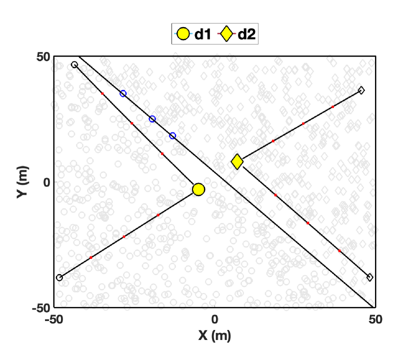
(a) $T=3$.

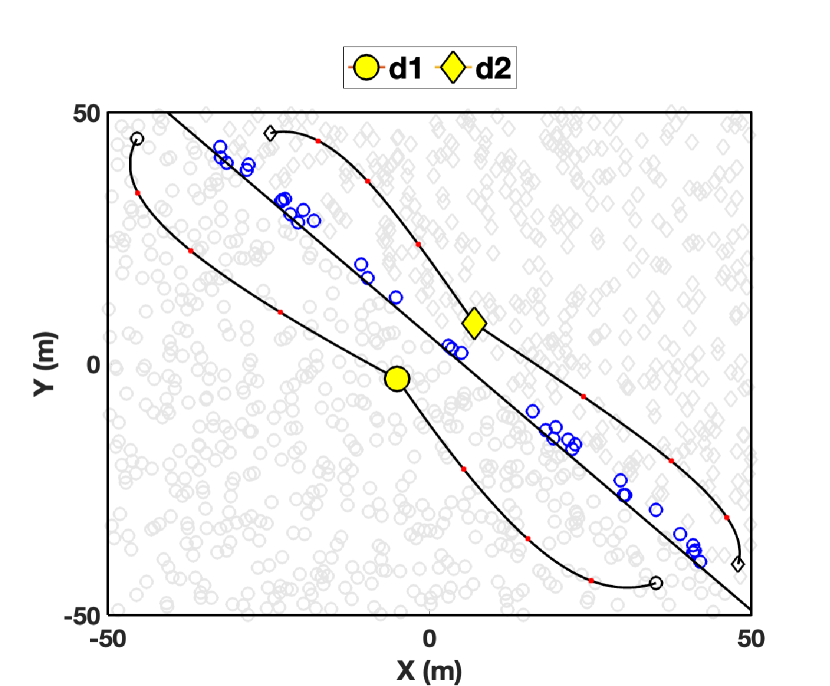
(b) $T=10$.

Figure 1: Agent trajectories and destinations choices, for $1000$ agents. Destinations are depicted by the yellow, black-contoured shapes. The central black line delineates destination choices under the continuum strategy. Grey, blue, and black markers indicate the agents’ initial positions, with their shapes corresponding to their chosen targets when employing the optimal strategy. The agents marked in blue are those whose optimal destination choice differs from that of the continuum strategy. Four agents and their corresponding trajectories are represented in black. Each trajectory displays three red dots, denoting the agents’ positions at instants $T/4$, $T/2$, and $3T/4$, respectively.

On Fig. 2, for two different populations sizes $100$ and $1000$, we plot the cost $J$ defined in (39), the average and standard deviation of the costs $J^{N}$ and $\tilde{J}^{N}$ from (27), (49), computed over 20 simulations and for a time horizon $T=3$. Running the Algorithm 2 gives that The optimal probability vector minimizing the cost $J$ is $[0.5535,0.4465]^{T}$. The costs $J^{N}$ and $\tilde{J}^{N}$ are evaluated on a probability grid with a discretization step of $0.1$. However, since agents employing the continuum strategy agents use the cells (42), the resulting agent-to-destination proportion $F^{N}(P)$ in (48) may exhibit slight deviations from the vector $P$. To reflect this, we choose to plot the average of the cost $\tilde{J}^{N}(P)$ against the average of the probability vectors $F^{N}(P)$, even though the cost $\tilde{J}^{N}(P)$ is computed as a function of $P$.

First, note that the cost function $J$ is a convex function, supporting the statement of Theorem 2. In addition, we observe that the standard deviation of the costs averages of $J^{N}$ and $\tilde{J}^{N}$, as well as the differences between the three costs, decrease with $N$, illustrating the convergence results of Section 5.1. Lastly, we observe that along the agent-to-destination proportion axis, the sign of $J^{N}(P)-\tilde{J}^{N}(P)$ varies. Indeed, when applying the continuum strategy for a finite population of size $N$, the actual agent-to-destination proportion is equal to $F^{N}(P)$ (See (48)). Consequently, $\tilde{J}^{N}(P)$ is the cost incurred for the agent-to-destination proportion $F^{N}(P)$, which may slightly differ from $P$. Therefore, in Fig.2, we observe that the sign of $J^{N}(P)-\tilde{J}^{N}(P)$ is correlated with the relative variation of the social cost $J(P)$ at the agent-to-destination proportions $P$ and $F^{N}(P)$. However, as the population size increases and $F^{N}(P)$ approaches $P$, such discrepancy diminishes.

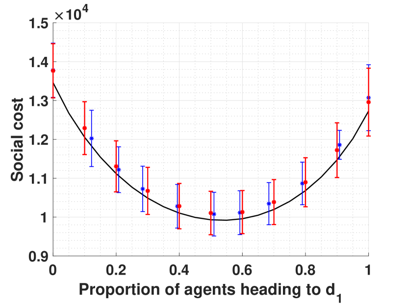
(a) $100$ agents.

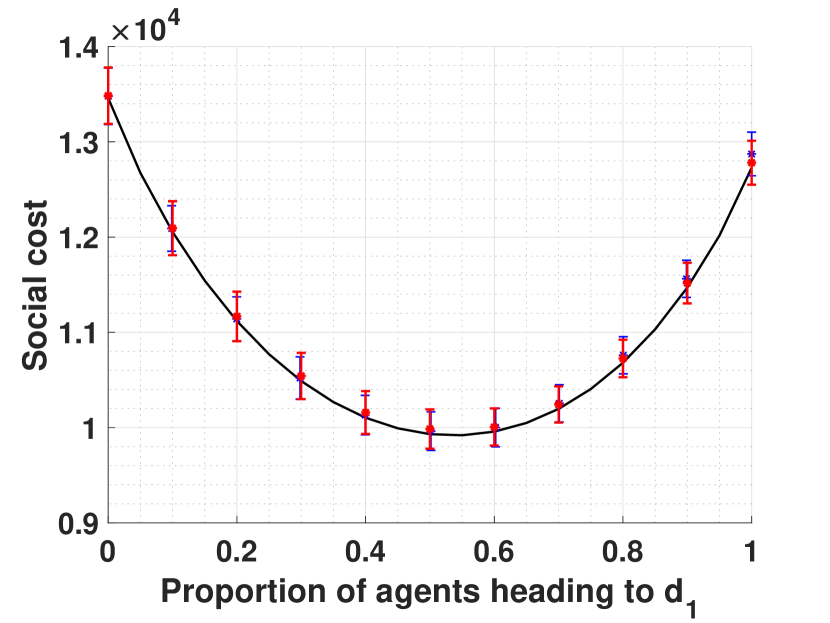
(b) $1000$ agents.

Figure 2: Costs $J$ ((39), black curve) $\tilde{J}^{N}$ ((49), in blue) and $J^{N}$ ((27), in red) for two populations.

7 Conclusion

This paper studies a linear quadratic collective discrete choice model. We account for congestion by introducing a negative term in the running cost. By exploiting the model’s symmetries, we derive the agents’ optimal control strategy. Since computing such strategy may be computationally expensive, we develop an $\varepsilon-$optimal decentralized control strategy, where $\varepsilon$ tends to zero as the population size increases. This strategy significantly reduces the required computation compared to its optimal counterpart, as well as the amount of inter-agent information exchange. In practice, the model may be useful for task assignment or ressource allocation in multi-agent systems. It is also of interest for future work to extend our analysis to agents with stochastic dynamics and to examine the case in which each agent can chose its exit time within the time interval $[0,T]$.

Appendix A Appendix

A.1 Proof of Lemma 1

To prove the lemma, we note that

$$\sum_{i=1}^{N}[x_{i}-\bar{x}^{N}]_{R_{x}}^{2}$$

$$=[X]^{2}_{R_{x}^{(N)}}-2(\bar{x}^{N})^{T}R_{x}\left(\sum_{i=1}^{N}x_{i}\right)+N[\bar{x}^{N}]_{R_{x}}^{2}$$

$$=[X]^{2}_{R_{x}^{(N)}}-N[\bar{x}^{N}]_{R_{x}}^{2}.$$

Moreover,

$$N[\bar{x}^{N}]_{R_{x}}^{2} =\frac{1}{N}\left(\sum_{i=1}^{N}x_{i}\right)^{T}R_{x}\left(\sum_{i=1}^{N}x_{i}\right)$$

$$=\frac{1}{N}((1_{N}^{T}\otimes I_{n})X)^{T}R_{x}((1_{N}^{T}\otimes I_{n})X)$$

$$=\frac{1}{N}X^{T}(1_{N}\otimes I_{n})R_{x}(1_{N}\otimes I_{n})^{T}X$$

$$\text{so }\quad N[\bar{x}^{N}]_{R_{x}}^{2} =\frac{1}{N}X^{T}\left(1_{NN}\otimes R_{x}\right)X.$$

Hence,

$$-\sum_{i=1}^{N}[x_{i}-\bar{x}^{N}]_{R_{x}}^{2}+\sum_{i=1}^{N}[x_{i}-d_{\lambda_{i}}]^{2}_{R_{d}}$$

$$=[X]^{2}_{-R_{x}^{(N)}+\frac{1}{N}\left(1_{NN}\otimes R_{x}\right)+R_{d}^{(N)}}-2d_{\lambda^{N}}^{T}R_{d}^{(N)}X+[{d_{\lambda^{N}}}]^{2}_{R_{d}^{(N)}},$$

and the rest of the argument leading to (4) is straightforward.

A.2 Proof of Lemma 3

Denote by $\pi(i,j)\in\mathbb{R}^{N\times N}$ the permutation matrix exchanging the $i^{th}$ and $j^{th}$ row of the identity matrix $I_{N}$, and let $\Pi(i,j)=\pi(i,j)\otimes I_{n}$. For $1\leq i,j\leq N$ denote by $\varphi^{N}_{ij}$ the $(i,j)$-block of size $n\times n$ of the matrix $\varphi^{N}\in\mathbb{R}^{Nn\times Nn}$, solution of (7). Note that for any matrix $M\in\mathbb{R}^{N\times N}$, $\pi(i,j)M$ exchanges the rows $i$ and $j$ of $M$ and $M\pi(i,j)$ exchanges the columns $i$ and $j$ of $M$. From this, one can see that the matrices $S^{(N)}$, $A^{(N)}$, $Q^{N}$ and $M^{(N)}$ appearing in (7) and (10) are left unchanged when multiplied by $\Pi(i,j)$ on the left and on the right. Moreover, note that $\Pi(i,j)=\Pi(i,j)^{T}=\Pi(i,j)^{-1}$. Hence, if $\varphi^{N}$ is a solution of (7), so is $\Pi(i,j)\varphi^{N}\Pi(i,j)$, for any $1\leq i,j\leq N$, and by unicity of the solution for the same terminal condition, all these matrices must be equal. This immediately implies that the diagonal blocks $\varphi^{N}_{ii}$ are all equal, for $1\leq i\leq N$, and the off-diagonal blocks $\varphi^{N}_{ij}$ for $j\neq i$, $1\leq i,j\leq N$, are also all equal. In other words, we can decompose $\varphi^{N}$ as in (13). Finally, rewriting (7) by block, we get (14) and (15).

A.3 Proof of Lemma 4

From (6), (8) and (10), we have that for any $i\in\llbracket N\rrbracket$,

$$\frac{d}{dt}\Psi^{N}_{i} =\left(\varphi^{N}_{1}S-A^{T}-\frac{1}{N}\varphi^{N}_{2}S\right)\Psi^{N}_{i}+R_{d}d_{\lambda_{i}}$$

$$+\frac{1}{N}\sum\limits_{j=1}^{N}\varphi^{N}_{2}S\Psi^{N}_{j},\;\;\Psi^{N}_{i}(T)=-Md_{\lambda_{i}}.$$ (55)

Hence, for any two agents $i,j\in\llbracket N\rrbracket$, we have

$$\frac{d}{dt}(\Psi^{N}_{i}-\Psi^{N}_{j})=\left(\varphi^{N}_{1}S-A^{T}-\frac{1}{N}\varphi^{N}_{2}S\right)(\Psi^{N}_{i}-\Psi^{N}_{j})$$

$$\;\;+R_{d}(d_{\lambda_{i}}-d_{\lambda_{j}}),\;\;(\Psi^{N}_{i}-\Psi^{N}_{j})(T)=-M(d_{\lambda_{i}}-d_{\lambda_{j}}).$$

Therefore, if $\lambda_{i}=\lambda_{j}$, i.e., the two agents have the same destination, then $0$ is a solution to this last differential equation and by unicity of the solution we get $\Psi^{N}_{i}=\Psi^{N}_{j}$. We then obtain the conclusion of Lemma 4, and (16) is obtained by grouping the terms of the sum in (55) by destination.

A.4 Proof of Lemma 5

Let’s assume that the solution of (16) is of the form (17). Let $\bar{\varphi}_{1}^{N}=\varphi^{N}_{1}S-A^{T}-\frac{1}{N}\varphi^{N}_{2}S$, and $\bar{\varphi}_{2}^{N}=\varphi^{N}_{2}S$. Injecting (17) in (16) and recalling $P_{D}^{N}=1-\sum_{j=1}^{D-1}P_{j}^{N}$, we obtain

$$\frac{d}{dt}\psi^{N}_{j} =\sum_{k=1}^{D-1}P^{N}_{k}\frac{d\alpha^{N}_{k}}{dt}-\frac{d\beta^{N}_{j}}{dt}$$

$$=\bar{\varphi}_{1}^{N}\left[\sum_{k=1}^{D-1}\alpha^{N}_{k}P^{N}_{k}-\beta^{N}_{j}\right]$$

$$\quad+\sum\limits_{k=1}^{D}P_{k}^{N}\bar{\varphi}_{2}^{N}\left[\sum_{l=1}^{D-1}\alpha^{N}_{l}P^{N}_{l}-\beta^{N}_{k}\right]+R_{d}d_{j}$$

$$\frac{d}{dt}\psi^{N}_{j} =\bar{\varphi}_{1}^{N}\left[\sum_{k=1}^{D-1}\alpha^{N}_{k}P^{N}_{k}-\beta^{N}_{j}\right]+R_{d}d_{j}$$

$$\quad+\sum\limits_{k=1}^{D-1}P_{k}^{N}\bar{\varphi}_{2}^{N}\left[\sum_{l=1}^{D-1}\alpha^{N}_{l}P^{N}_{l}-\beta^{N}_{k}\right]$$

$$\quad+\left(1-\sum\limits_{k=1}^{D-1}P_{k}^{N}\right)\bar{\varphi}_{2}^{N}\left[\sum_{l=1}^{D-1}\alpha^{N}_{l}P^{N}_{l}-\beta^{N}_{D}\right]$$

so finally

$$\frac{d}{dt}\psi^{N}_{j} =\sum_{k=1}^{D-1}P^{N}_{k}\left[(\bar{\varphi}_{1}^{N}+\bar{\varphi}_{2}^{N})\alpha^{N}_{k}+\bar{\varphi}_{2}^{N}(\beta_{D}^{N}-\beta_{k}^{N})\right]$$

$$\quad-\bar{\varphi}_{1}^{N}\beta^{N}_{j}-\bar{\varphi}_{2}^{N}\beta^{N}_{D}+R_{d}d_{j},$$

with $\sum_{k=1}^{D-1}\alpha^{N}_{k}(T)P^{N}_{k}+\beta^{N}_{j}(T)=Md_{j}$ as terminal condition. By identifying the terms, we get that the coefficients $\alpha^{N}_{j}$ and $\beta^{N}_{j}$ should respectively satisfy the linear differential equations (18) and (19), for which a unique solution exists. Consequently, the solution candidate (17) satisfies the relation (16). By unicity of the solution to the linear differential equation (16), we conclude that (17) is the solution for (16).

A.5 Proof of Lemma 6

Note that from (17) and the definition (LABEL:eq:_alphaN_matrix), we have $\psi_{j}^{N}(t)=\alpha^{N}(t)P^{N}-\beta^{N}_{j}(t)$. We then use the result of Lemma 4 and inject (17) in (9) to get

$$\frac{d}{dt}\chi^{N}=\frac{1}{2}\sum\limits_{j=1}^{D}P_{j}^{N}\left([\psi_{j}^{N}]^{2}_{S}-[d_{j}]^{2}_{R_{d}}\right)$$

$$\frac{d}{dt}\chi^{N}=\frac{1}{2}\sum\limits_{j=1}^{D}P_{j}^{N}\left(\left[\alpha^{N}P^{N}-\beta_{j}^{N}\right]^{2}_{S}-[d_{j}]^{2}_{R_{d}}\right)$$

$$=\frac{1}{2}(P^{N})^{T}(\alpha^{N})^{T}S\alpha^{N}P^{N}-\sum_{j=1}^{D}P^{N}_{j}(\beta^{N}_{j})^{T}S\alpha^{N}P^{N}$$

$$+\frac{1}{2}\sum_{j=1}^{D}P_{j}^{N}\left([\beta_{j}^{N}]^{2}_{S}-[d_{j}]^{2}_{R_{d}}\right)$$

$$\frac{d}{dt}\chi^{N}=(P^{N})^{T}W^{N}P^{N}+\frac{1}{2}\sum_{j=1}^{D}P_{j}^{N}\left([\beta_{j}^{N}]^{2}_{S}-[d_{j}]^{2}_{R_{d}}\right),$$

with $W^{N}$ defined in (22).

A.6 Proof of Lemma 7

Using (5) and (17), we have that

$$V^{N}(t,\lambda^{N})=\frac{1}{2N}X^{T}\varphi^{N}X+\frac{1}{N}(\Psi^{N})^{T}X+\chi^{N}$$

$$=\frac{1}{2N}\left(\sum_{i=1}^{N}x_{i}^{T}\varphi_{1}^{N}x_{i}+\sum_{i=1}^{N}\sum_{\begin{subarray}{c}j=1\\ j\neq i\end{subarray}}^{N}\frac{1}{N}x_{i}^{T}\varphi_{2}^{N}x_{j}\right)$$

$$+\frac{1}{N}\sum\limits_{i=1}^{N}\left(\left(\sum_{j=1}^{D-1}P^{N}_{j}\alpha^{N}_{j}\right)-\beta^{N}_{\lambda_{i}}\right)^{T}x_{i}+\chi^{N}(t)$$

$$=\frac{1}{2N}\sum_{i=1}^{N}x_{i}^{T}\varphi_{1}^{N}x_{i}+\frac{1}{2}\left(\frac{1}{N}\sum_{i=1}^{N}x_{i}\right)^{T}\varphi_{2}^{N}\left(\frac{1}{N}\sum_{i=1}^{N}x_{i}\right)$$

$$-\frac{1}{2N^{2}}\sum_{i=1}^{N}x_{i}^{T}\varphi_{2}^{N}x_{i}+\frac{1}{N}\sum\limits_{i=1}^{N}\left(\sum\limits_{j=1}^{D-1}P^{N}_{j}(\alpha_{j}^{N})^{T}x_{i}\right.$$

$$\left.+\frac{1}{2}\left(|x_{i}-\beta_{\lambda_{i}}^{N}|_{2}^{2}-|x_{i}|_{2}^{2}-|\beta_{\lambda_{i}}^{N}|_{2}^{2}\right)\right)+\chi^{N}(t)$$

$$V^{N}(t,\lambda^{N}) =\frac{1}{2N}\sum_{i=1}^{N}x_{i}^{T}\left(\varphi_{1}^{N}-\frac{\varphi_{2}^{N}}{N}\right)x_{i}+\frac{1}{2}(\bar{x}^{N})^{T}\varphi_{2}^{N}\bar{x}^{N}$$

$$+\sum\limits_{j=1}^{D-1}P^{N}_{j}(\alpha_{j}^{N})^{T}\bar{x}^{N}-\frac{1}{2}\sum\limits_{j=1}^{D}P^{N}_{j}|\beta_{j}^{N}|_{2}^{2}$$

$$+\frac{1}{2N}\sum\limits_{i}=1^{N}|x_{i}-\beta_{\lambda_{i}}^{N}|_{2}^{2}-\frac{1}{2N}\sum\limits_{i=1}^{N}|x_{i}|_{2}^{2}+\chi^{N}(t).$$

A.7 Proof of Theorem 1

Define the matrix $Q_{\min}^{N}=I_{N}\otimes(R_{d}-R_{x})$, so that

$$Q^{N}-Q_{\min}^{N} =\frac{1}{N}1_{NN}\otimes R_{x}.$$

The eigenvalues of the Kronecker product of any two square matrices are the pairwise products of the eigenvalues of both matrices. The only non-zero eigenvalue of the rank $1$ matrix $\frac{1}{N}1_{NN}$ is $1$. Since $R_{x}$ is positive definite, we conclude that $Q_{\min}^{N}\preccurlyeq Q^{N}$. Therefore, by using the order preserving property for Hermitian Riccati equations [15, Theorem 4.1.4], we conclude that $\Delta_{esc}(Q_{\min}^{N})\leq\Delta_{esc}(Q^{N})$, where, to simplify the notation, we have redefined $\Delta_{esc}(\tilde{Q})=\Delta_{esc}(S^{(N)},A^{(N)},\tilde{Q},M^{(N)})$, for $\tilde{Q}\in\mathbb{R}^{Nn\times Nn}$ symmetric.

Suppose now that $T<\Delta_{esc}(Q_{\min}^{N})$. Then

$$T-\Delta_{esc}(Q^{N})\leq T-\Delta_{esc}(Q_{\min}^{N})<0,$$

so the Riccati equation (7) has a solution over the time interval $[0,T]$. Finally, since all the matrices in $\textit{HDRE}(T,S^{(N)},A^{(N)},Q_{\min}^{N},M^{(N)})$ are block diagonal with repeated diagonal blocks, we have that $\Delta_{esc}(Q_{\min}^{N})=\Delta_{esc}(S,A,R_{d}-R_{x},M)$. This gives the sufficient condition of the theorem.

A.8 Proof of Lemma 9

Define $c(x,j)=|x-\beta_{j}(0)|^{2}$, for any $x$ in $E$ and $j\in\llbracket D\rrbracket$. By Kantorovitch duality [19, Theorem 5.10], we can write for the OT problem (38)

$$C(P)=\max_{(\phi,g)\in\Phi^{c}}\int_{E}\phi(x)d\mathcal{P}_{0}(x)+\sum_{j=1}^{D}P_{j}g_{j},$$ (56)

where, denoting $\overline{\mathbb{R}}=\mathbb{R}\cup\{-\infty\}$, we have

$$\Phi^{c}=\Big{\{}\phi:\mathbb{R}^{n}\to\overline{\mathbb{R}},g\in\overline{\mathbb{R}}^{D}:\int_{E}|\phi(x)|d\mathcal{P}_{0}(x)<\infty,$$ (57)

$$\sum_{j=1}^{D}|g_{j}|P_{j}<\infty;\phi(x)+g_{j}\leq c(x,j),\forall x\in E,\forall j\in\llbracket D\rrbracket\Big{\}}.$$

The notation $\max$ in (56) means that an maximizing pair $(\tilde{\phi},\tilde{g})$ in $\Phi^{c}$ exists. However, the summability condition on $g$ in (57) does not rule out a priori that $\tilde{g}_{j}=-\infty$ when $P_{j}=0$, see Remark 1. Nonetheless, due to the inequality constraint in $\Phi^{c}$, starting from $\tilde{\phi}$, $\tilde{g}$, we can replace $\tilde{\phi}$ by its $c$-transform [19], defined for all $x$ in $E$ as

$$\phi^{*}(x)\coloneqq\min_{j\in\llbracket D\rrbracket}\{c(x,j)-g^{*}_{j}\}=\min_{j:g^{*}_{j}>-\infty}\{c(x,j)-g^{*}_{j}\},$$ (58)

without reducing the cost in (56). In (58) the elements $g_{j}^{*}=-\infty$ lead to $c(x,j)-g_{j}^{*}$ and hence can be removed from the minimization. Note that this leads to the form (40) for the dual function, but more importantly here, $\phi^{*}$ is continuous because $c(\cdot,j)$ is continuous for each $j\in\llbracket D\rrbracket$. Similarly, we can then replace $\tilde{g}$ by its $c$-transform $g^{*}$, with components

$$g^{*}_{j}=\inf_{x\in E}\{c(x,j)-\phi^{*}(x)\},\;\;j\in\llbracket D\rrbracket,$$ (59)

without reducing the cost in (56). But since $\phi^{*}$ is continuous, $c(\cdot,j)$ is continuous, and $E$ is compact by Assumption 2, the infimum is attained in (59) and $g^{*}_{j}$ is finite, for each $j\in\llbracket D\rrbracket$. This proves the second part of the lemma, i.e., $g^{*}\in\mathbb{R}^{D}$ is an maximizer of the dual function.

For the first part, $g\mapsto J^{D}(g,P)$ is concave as a general property of dual functions, or more directly one can observe that $\min_{j}\{c(x,j)-g_{j}\}$ is concave in $g$ as the minimum of linear functions, and concavity is preserved by integration.

A.9 Proof of Lemma 11

Recall first the definition of the Wasserstein $2$-distance between two measures $\mu$ and $\nu$ on $\mathbb{R}^{n}$

$$W_{2}(\mu,\nu)=\left(\inf_{\gamma\in\Gamma(\mu,\nu)}\int_{\mathbb{R}^{n}\times\mathbb{R}^{n}}|x-y|_{2}^{2}\;d\gamma(x,y)\right)^{1/2},$$

where $\Gamma(\mu,\nu)$ is the set of all joint measures in $\mathcal{M}(\mathbb{R}^{n}\times\mathbb{R}^{n})$ with marginals $\mu$ and $\nu$, i.e.,

$$\gamma(A\times\mathbb{R}^{n})=\mu(A),\;\;\gamma(\mathbb{R}^{n}\times B)=\nu(B),$$

for all measurable sets $A$ and $B$.

Define, for any $P\in\Omega$, the probability measure $\mathcal{P}_{T}(P)=\sum_{i=1}^{D}P_{i}\delta_{\beta_{i}(0)}$ on $\mathbb{R}^{n}$, where $\delta_{x}$ denotes the Dirac measure at $x$. Notice from (38) that

$$C\left(P\right)=W_{2}\left(\mathcal{P}_{0},\mathcal{P}_{T}(P)\right)^{2}.$$

Consider a sequence $\{P^{(n)}\}_{n\geq 0}$ in $\Omega$ converging to some vector $P\in\Omega$. Then $\mathcal{P}_{T}(P^{(n)})$ converges weakly to $\mathcal{P}_{T}(P)$, so by [19, Theorem 6.9], under Assumption 2, $\lim_{n\to\infty}C(P^{(n)})\to C(P)$, which shows the continuity of $C$ on $\Omega$.

For the convexity of $C$, consider two vectors $P^{1},P^{2}$ in $\Omega$ and $\lambda\in[0,1]$. The cost function $c(x,y)=|x-y|_{2}^{2}$ is continuous and non-negative on $\mathbb{R}^{n}\times\mathbb{R}^{n}$. Define the discrete measure $\Lambda$ on the set $\{1,2\}$ by $\Lambda(\{1\})=\lambda$, $\Lambda(\{2\})=1-\lambda$.

According to [19, Theorem 4.8], we then have

$$C(\lambda P^{1}+(1-\lambda)P^{2})\leq\lambda C(P^{1})+(1-\lambda)C(P^{2}),$$

i.e., $C$ is convex on $\Omega$.

A.10 Proof of Lemma 12

By integrating (34), we have

$$\chi(0,P) =\chi(T,P)-P^{T}\left(\int_{0}^{T}W(\tau)d\tau\right)P$$

$$-\frac{1}{2}\sum_{j=1}^{D}P_{j}\int_{0}^{T}[\beta_{j}(\tau)]^{2}_{S}-[d_{j}]^{2}_{R_{d}}d\tau.$$

Since $\chi(T,P)$ is linear in $P$, to prove the convexity of $\chi(0,P)$ on $\Omega$ it is sufficient to prove that $P\to P^{T}W(t)P$ is concave on $\Omega$, for all $t$. Let us parametrize $\Omega$ as

$$\tilde{\Omega}=\{ \begin{bmatrix}P_{1}\ldots P_{D-1}\end{bmatrix}^{T}\in\mathbb{R}^{D-1}\Big{|}$$

$$P_{i}\geq 0,\forall i\in\llbracket D-1\rrbracket,\sum_{i=1}^{D-1}P_{i}\leq 1\},$$

so $P\in\Omega$ if and only if $P=\begin{bmatrix}\tilde{P}^{T},(1-1_{D-1}^{T}\tilde{P})\end{bmatrix}^{T}$ for $\tilde{P}\in\tilde{\Omega}$. Let $\tilde{\alpha}=\begin{bmatrix}\alpha_{1}\ldots\alpha_{D-1}\end{bmatrix}$, $\tilde{\beta}=\begin{bmatrix}\beta_{1}\ldots\beta_{D-1}\end{bmatrix}$. Note that

$$W=\begin{bmatrix}\tilde{W}&0_{(D-1)\times 1}\\ -\beta_{D}^{T}S\tilde{\alpha}&0\end{bmatrix},\;\;\tilde{W}=\left(\frac{\tilde{\alpha}}{2}-\tilde{\beta}\right)^{T}S\tilde{\alpha},$$

and, for $P=\begin{bmatrix}\tilde{P}^{T},(1-1_{D-1}^{T}\tilde{P})\end{bmatrix}^{T}$,

$$P^{T}WP=\tilde{P}\left(\tilde{W}+1_{D-1}\beta_{D}^{T}S\tilde{\alpha}\right)\tilde{P}-\beta_{D}^{T}S\tilde{\alpha}\tilde{P}.$$

As a result, the function is $P\to P^{T}WP$ is concave on $\Omega$ if the symmetric part of the matrix

$$\tilde{W}+1_{D-1}\beta_{D}^{T}S\tilde{\alpha}=\left(\tilde{\alpha}-\left(\tilde{\beta}-\beta_{D}1_{D-1}^{T}\right)\right)^{T}S\tilde{\alpha}-\frac{1}{2}\tilde{\alpha}^{T}S\tilde{\alpha}$$ (60)

is negative semi-definite.

Let $d=[d_{1}-d_{D},\ldots,d_{D-1}-d_{D}]\in\mathbb{R}^{n\times(D-1)}$. Let $\bar{\varphi}_{1}=\varphi_{1}S-A^{T}$, $\bar{\varphi}_{2}=\varphi_{2}S$ and let $\Phi_{\bar{\varphi}_{1}}$ and $\Phi_{\bar{\varphi}_{1}+\bar{\varphi}_{2}}$ be the state transition matrices of $\bar{\varphi}_{1}$ and $\bar{\varphi}_{1}+\bar{\varphi}_{2}$ respectively. From (32), we have for all $j\in\llbracket D-1\rrbracket$

$$\frac{d}{dt}(\beta_{j}-\beta_{D}) =\bar{\varphi}_{1}(\beta_{j}-\beta_{D})-R_{d}(d_{j}-d_{D}),$$

$$(\beta_{j}-\beta_{D})(T) =M(d_{j}-d_{D}).$$ (61)

Therefore,

$$\tilde{\beta}(t)-\beta_{D}(t)1_{D-1}^{T}=\bar{\phi}_{\beta}(t)\,d,$$ (62)

with

$$\bar{\phi}_{\beta}(t)=\int_{t}^{T}\Phi_{\bar{\varphi}_{1}}(t,\tau)R_{d}\,d\tau+\Phi_{\bar{\varphi}_{1}}(t,T)M.$$

By substracting (61) from (31), we get that for all $j\in\llbracket D-1\rrbracket$,

$$\frac{d}{dt}\left(\alpha_{j}-(\beta_{j}-\beta_{D})\right)=(\bar{\varphi}_{1}+\bar{\varphi}_{2})\left(\alpha_{j}-(\beta_{j}-\beta_{D})\right)$$

$$\;\;+R_{d}(d_{j}-d_{D})\;,\;\left(\alpha_{j}-(\beta_{j}-\beta_{D})\right)(T)=-M(d_{j}-d_{D}).$$

Hence,

$$\tilde{\alpha}(t)-\left(\tilde{\beta}(t)-\beta_{D}(t)1_{D-1}^{T}\right) =-\bar{\phi}_{\alpha-\beta}(t)\,d,$$

with

$$\bar{\phi}_{\alpha-\beta}(t)=\int_{t}^{T}\Phi_{\bar{\varphi}_{1}+\bar{\varphi}_{2}}(t,\tau)R_{d}d\tau+\Phi_{\bar{\varphi}_{1}+\bar{\varphi}_{2}}(t,T)M.$$

From (31) and (62), we establish the following

$$\tilde{\alpha}(t) =-\int_{T}^{t}\Phi_{\bar{\varphi}_{1}+\bar{\varphi}_{2}}(t,\tau)\,\bar{\varphi}_{2}(\tau)\left(\tilde{\beta}-\beta_{D}1_{D-1}^{T}\right)(\tau)d\tau$$

$$=\left(\int_{t}^{T}\Phi_{\bar{\varphi}_{1}+\bar{\varphi}_{2}}(t,\tau)\bar{\varphi}_{2}(\tau)\bar{\phi_{\beta}}(\tau)d\tau\right)d=:\bar{\phi}_{\alpha}(t)\,d.$$

Let us call a diagonal matrix with all nonnegative or all positive diagonal coefficients a diagonal nonnegative or positive matrix respectively. Under Assumption 4, $S$ is a diagonal nonnegative matrix. Furthermore, under Assumption 4 and using [15, Theorem 4.1.6], we can show that the solution $\varphi_{2}$ of the Riccati equation (30) is a diagonal nonnegative matrix. Therefore, $\bar{\varphi}_{2}$ is a diagonal nonnegative matrix. Besides, any state transition matrix of a diagonal matrix is a diagonal positive matrix. Therefore, since the matrices $A,B,R_{X},R_{d},R_{u},M$ are diagonal, the matrices $\bar{\phi}_{\alpha-\beta}$, $\bar{\phi}_{\beta}$ and $\bar{\phi}_{\alpha}$ are diagonal nonnegative matrices. As a result, $\bar{\phi}_{\alpha-\beta}^{T}S\bar{\phi}_{\alpha}$ is a diagonal nonnegative matrix and so, from (60),

$$\tilde{W}(t)+1_{D-1}\beta_{D}^{T}(t)S\tilde{\alpha}(t) =-d^{T}\bar{\phi}_{\alpha-\beta}^{T}S\bar{\phi}_{\alpha}d-\frac{1}{2}\tilde{\alpha}^{T}S\tilde{\alpha}$$

is a negative semi-definite matrix, for all $t\in[0,T]$. Hence, the function $P\rightarrow\chi(0,P)$ is convex under Assumption 4.

A.11 Proof of Lemma 13

For any $P\in\Omega$, we have from (LABEL:eq:_J_bar_N) and (39)

$$\bar{J}^{N}(P)-J(P)=$$

$$\frac{1}{2}\left(\Delta^{N}_{I}(P)+\Delta^{N}_{II}(P)+\Delta^{N}_{III}+\Delta^{N}_{IV}+\Delta^{N}_{V}+\Delta_{VI}\right),$$

with

$$\Delta^{N}_{I}(P)=\bar{C}^{N}(P)-C(P),\;\;\Delta^{N}_{II}(P)=\chi^{N}(0,P)-\chi(0,P),$$

$$\Delta^{N}_{III}=\int_{x\in E}|x|^{2}d\mathcal{P}_{0}(x)-\frac{1}{N}\sum\limits_{i=1}^{N}|x_{i}(0)|^{2},$$

$$\Delta^{N}_{IV} =\frac{1}{N}\sum_{i=1}^{N}x_{i}(0)^{T}\left(\varphi^{N}_{1}(0)-\frac{\varphi^{N}_{2}(0)}{N}\right)x_{i}(0)$$

$$-\int_{x\in E}x^{T}\varphi_{1}(0)x\,d\mathcal{P}_{0}(x),$$

$$\Delta^{N}_{V}=\bar{x}^{N}(0)^{T}\varphi^{N}_{2}(0)\bar{x}^{N}(0)-\bar{x}(0)^{T}\varphi_{2}(0)\bar{x}(0),$$

$$\Delta^{N}_{VI} =\sum_{j=1}^{D-1}2P_{j}\left(\alpha^{N}_{j}(0)^{T}\bar{x}^{N}(0)-\alpha_{j}(0)^{T}\bar{x}(0)\right)$$

$$+\sum_{j=1}^{D}P_{j}\left(|\beta_{j}(0)|_{2}^{2}-|\beta_{j}^{N}(0)|_{2}^{2}\right).$$

By the strong law of large numbers (SLLN), $\Delta^{N}_{III}\to 0$ as $N\to\infty$, almost surely. We also have the following results.

Lemma 18

The functions $\varphi^{N}_{1}$, $\varphi^{N}_{2}$, $\alpha^{N}_{j}$, $j\in\llbracket D-1\rrbracket$ and $\beta^{N}_{j}$, $j\in\llbracket D\rrbracket$, solutions to (14), (15), (15), (18), converge uniformly on $[0,T]$ to the solutions $\varphi_{1}$, $\varphi_{2}$, $\alpha_{j}$ and $\beta_{j}$ of (29), (30), (31), (32) respectively, as $N\to\infty$.

Lemma 19

Almost surely, the function $P\mapsto\Delta^{N}_{I}(P)$ converges uniformly to $0$ on $\Omega$ as $N\to\infty$.

Lemma 20

The functions $W^{N}$ defined in (22) and $[\beta^{N}_{j}]_{S}^{2}$, $j\in\llbracket D\rrbracket$ converge uniformly on $[0,T]$ to $W$ defined in (33) and $[\beta_{j}]_{S}^{2}$ respectively, as $N\to\infty$.

Lemma 21

The function $P\mapsto\Delta_{II}^{N}(P)$ converges uniformly to $0$ on $\Omega$ as $N\to\infty$.

Using Lemma 18 and the SLLN, it is straightforward to show that almost surely, $\Delta^{N}_{IV}$, $\Delta^{N}_{V}$ and $\Delta_{VI}^{N}$ converge to $0$ as $N\to\infty$. Hence, with Lemma 19 and Lemma 21, we conclude that with probability one, $\bar{J}^{N}$ converges uniformly to $J$ on $\Omega$. This proves Lemma 13. The rest of the section contains the proofs of Lemmas 18, 19, 20 and 21.

A.11.1 Proof of Lemma 18

For each $N$, the functions $\varphi^{N}_{1}$, $\varphi^{N}_{2}$, $\alpha^{N}_{j}$, $j\in\llbracket D-1\rrbracket$ and $\beta^{N}_{j}$, $j\in\llbracket D\rrbracket$, form the solution $t\to\xi^{N}(t)\in\mathbb{R}^{2n^{2}+(2D-1)n}$ to the system of ordinary differential equations (ODEs) (14), (15), (18) and (19), which we can rewrite as $\dot{\xi}^{N}=f^{N}(\xi^{N})$, with $\xi^{N}(T)=\xi_{T}$, for some function $f^{N}$. Similarly, the functions $\varphi_{1}$, $\varphi_{2}$, $\alpha_{j}$, $j\in\llbracket D-1\rrbracket$ and $\beta_{j}$, $j\in\llbracket D\rrbracket$ form the solution $t\to\xi(t)$ to the system of ODEs (29), (30), (31), (32), which we can rewrite as $\dot{\xi}=f(\xi)$, with $\xi(T)=\xi_{T}$, for some function $f$. Note that these two systems have the same terminal conditions. It is straightforward to see that as $N\to\infty$, $f^{N}$ converges uniformly on compacts to $f$. Moreover, the solution to the limit system $\dot{\xi}=f(\xi)$, $\xi(T)=\xi_{T}$, is unique by the standard properties of Riccati and linear ODEs. Hence, by [25, Theorem 3], we conclude that $t\to\xi^{N}(t)$ converges uniformly on $[0,T]$ to $t\to\xi(t)$ and $N\to\infty$.

A.11.2 Proof of Lemma 19

Recall first the definitions given at the beginning of Appendix A.9. For any $P\in\Omega$ and any initial conditions $x_{1}(0),x_{2}(0),\ldots,$ sampled independently according to $\mathcal{P}_{0}$, define the probability measures

$$\mathcal{P}^{N}_{0} =\sum_{i=1}^{N}\frac{1}{N}\delta_{x_{i}(0)},$$ (63)

$$\mathcal{P}^{N}_{T}(P) =\sum_{i=1}^{D}P_{i}\delta_{\beta^{N}_{i}(0)},\text{ and }\mathcal{P}_{T}(P)=\sum_{i=1}^{D}P_{i}\delta_{\beta_{i}(0)}$$

on $\mathbb{R}^{n}$. To simplify the notation we sometimes omit the argument $P$ from $\mathcal{P}^{N}_{T}$ and $\mathcal{P}_{T}$ in the following. With the definitions (LABEL:eq:_discrete_Kantorovich_prime) and (38), we have

$$\bar{C}^{N}\left(P\right)=W_{2}\left(\mathcal{P}^{N}_{0},\mathcal{P}^{N}_{T}\right)^{2}\text{ and }C\left(P\right)=W_{2}\left(\mathcal{P}_{0},\mathcal{P}_{T}\right)^{2},$$

and so

$$|\bar{C}^{N}\left(P\right)-C\left(P\right)| =|W_{2}\left(\mathcal{P}^{N}_{0},\mathcal{P}^{N}_{T}\right)-W_{2}\left(\mathcal{P}_{0},\mathcal{P}_{T}\right)|\times$$

$$\left(W_{2}\left(\mathcal{P}^{N}_{0},\mathcal{P}^{N}_{T}\right)+W_{2}\left(\mathcal{P}_{0},\mathcal{P}_{T}\right)\right).$$ (64)

In the following, we show that the right-hand side of (64) converges uniformly on $\Omega$ to $0$, almost surely, by considering each term in the product.

Since $W_{2}$ defines a distance between probability measures with finite second moment [19, Chapter 6], by the triangle inequality

$$W_{2}\left(\mathcal{P}^{N}_{0},\mathcal{P}^{N}_{T}\right)- W_{2}\left(\mathcal{P}_{0},\mathcal{P}_{T}\right)\leq$$

$$W_{2}\left(\mathcal{P}^{N}_{0},\mathcal{P}_{0}\right)+W_{2}\left(\mathcal{P}_{T},\mathcal{P}^{N}_{T}\right).$$

Similarly,

$$W_{2}\left(\mathcal{P}_{0},\mathcal{P}_{T}\right)- W_{2}\left(\mathcal{P}^{N}_{0},\mathcal{P}^{N}_{T}\right)\leq$$

$$W_{2}\left(\mathcal{P}_{0},\mathcal{P}^{N}_{0}\right)+W_{2}\left(\mathcal{P}^{N}_{T},\mathcal{P}_{T}\right).$$

Hence, by the symmetry property of the distance,

$$|W_{2}\left(\mathcal{P}^{N}_{0},\mathcal{P}^{N}_{T}\right)- W_{2}\left(\mathcal{P}_{0},\mathcal{P}_{T}\right)|\leq$$ (65)

$$W_{2}\left(\mathcal{P}^{N}_{0},\mathcal{P}_{0}\right)+W_{2}\left(\mathcal{P}^{N}_{T},\mathcal{P}_{T}\right).$$

By considering the transportation plan sending all the mass $P_{i}$ at $\beta^{N}_{i}(0)$ to $\beta_{i}(0)$, we obtain that

$$W_{2}\left(\mathcal{P}^{N}_{T},\mathcal{P}_{T}\right) \leq\sqrt{\sum_{i=1}^{D}P_{i}|\beta^{N}_{i}(0)-\beta_{i}(0)|_{2}^{2}}$$

$$\leq\sqrt{\sum_{i=1}^{D}|\beta^{N}_{i}(0)-\beta_{i}(0)|_{2}^{2}},$$

using the fact that $P_{i}\leq 1$, for all $i\in\llbracket D\rrbracket$. Hence, from Lemma 18,

$$\lim_{N\to\infty}\sup_{P\in\Omega}W_{2}\left(\mathcal{P}^{N}_{T},\mathcal{P}_{T}\right)=0.$$ (66)

The random measure $\mathcal{P}_{0}^{N}$ converges weakly to $\mathcal{P}_{0}$, almost surely [26]. Hence, by [19, Theorem 6.9] and under Assumption 3,

$$\lim_{N\to\infty}W_{2}(\mathcal{P}_{0}^{N},\mathcal{P}_{0})=0,\;\text{almost surely}.$$ (67)

Combining (67) with (66) in (65) shows that almost surely,

$$\lim_{N\to\infty}\sup_{P\in\Omega}|W_{2}\left(\mathcal{P}^{N}_{0},\mathcal{P}^{N}_{T}\right)-W_{2}\left(\mathcal{P}_{0},\mathcal{P}_{T}\right)|=0.$$ (68)

For the other term in the product (64), by the triangle inequality again

$$W_{2}\left(\mathcal{P}^{N}_{0},\mathcal{P}^{N}_{T}\right)+W_{2}\left(\mathcal{P}_{0},\mathcal{P}_{T}\right)$$

$$\leq W_{2}\left(\mathcal{P}^{N}_{0},\mathcal{P}_{0}\right)+2W_{2}\left(\mathcal{P}_{0},\mathcal{P}_{T}\right)+W_{2}\left(\mathcal{P}_{T},\mathcal{P}^{N}_{T}\right).$$

By (66) and (67), almost surely, there exists some constant $c_{1}$ and some integer $N_{0}$ such that for all $N\geq N_{0}$,

$$W_{2}\left(\mathcal{P}^{N}_{0},\mathcal{P}_{0}\right)+\sup_{P\in\Omega}W_{2}\left(\mathcal{P}_{T},\mathcal{P}^{N}_{T}\right)\leq c_{1}.$$

Finally, by [19, Corollary 6.10], $P\mapsto W_{2}\left(\mathcal{P}_{0},\mathcal{P}_{T}(P)\right)$ is a continuous function of $P$ on $\Omega$, which is compact, hence it is uniformly bounded on $\Omega$. We conclude from that almost surely, the term $W_{2}\left(\mathcal{P}^{N}_{0},\mathcal{P}^{N}_{T}\right)+W_{2}\left(\mathcal{P}_{0},\mathcal{P}_{T}\right)$ in (64) is uniformly bounded on $\Omega$ for $N$ large enough, and hence with (68) obtain the result of the lemma, i.e.,

$$\lim_{N\to\infty}\sup_{P\in\Omega}|\bar{C}^{N}(P)-C(P)|=0,\text{ almost surely}.$$

A.11.3 Proof of Lemma 20

The coefficients $\alpha_{j}$ and $\beta_{j},j\in\llbracket D-1\rrbracket$ are solution of the differential equations (31), (32) respectively. Therefore, they are bounded over the time interval $[0,T]$. By the uniform convergence of the coefficients $\alpha_{j}^{N}$ and $\beta_{j}^{N}$ to $\alpha_{j}$ and $\beta_{j},j\in\llbracket D-1\rrbracket$ with respect to $t\in[0,T]$, we establish that $W^{N}$ defined in (22), $\alpha_{j}^{N}$, and $\beta_{j}^{N},j\in\llbracket D-1\rrbracket$ are uniformly bounded. Since the product of bounded uniformly convergent functions is uniformly convergent [27, Exercise 2], we conclude from Lemma 18 that the functions $W^{N}$ and $[\beta^{N}_{j}]_{S}^{2}$ converge uniformly on $[0,T]$ to $W$ defined in (33) and $[\beta_{j}]_{S}^{2}$ respectively, with $j\in\llbracket D\rrbracket$.

A.11.4 Proof of Lemma 21

We need to show that $\chi^{N}(0,\cdot)$ converges uniformly to $\chi(0,\cdot)$ on $\Omega$, with $\chi^{N}$ and $\chi$ the solutions of (21) and (34). Let $\Delta^{N}_{\chi}(t,P)=\chi(t,P)-\chi^{N}(t,P)$. First, $\Delta^{N}_{\chi}(T,P)=0$.

Then, denoting by $\|\cdot\|_{2}$ the induced $2$-norm,

$$\left|\frac{\partial}{\partial t}\Delta^{N}_{\chi}(t,P)\right|$$

$$=\left|P^{T}(W-W^{N})P+\frac{1}{2}\sum_{j=1}^{D}P_{j}\left([\beta_{j}]^{2}_{S}-[\beta_{j}^{N}]^{2}_{S}\right)\right|$$

$$\leq\|W-W^{N}\|_{2}\;|P|_{2}^{2}+\frac{1}{2}\sum_{j=1}^{D}P_{j}\left|[\beta_{j}]^{2}_{S}-[\beta^{N}_{j}]^{2}_{S}\right|$$

$$\leq\|W(t)-W^{N}(t)\|_{2}+\frac{1}{2}\sum_{j=1}^{D}|[\beta_{j}(t)]^{2}_{S}-[\beta^{N}_{j}(t)]^{2}_{S}|.$$

Therefore,

$$|\Delta_{\chi}(0,P)| \leq\int_{0}^{T}\|W(\tau)-W^{N}(\tau)\|_{2}d\tau$$

$$+\frac{1}{2}\sum_{j=1}^{D}\int_{0}^{T}\left|[\beta_{j}(\tau)]^{2}_{S}-[\beta^{N}_{j}(\tau)]^{2}_{S}\right|d\tau.$$ (69)

The upper bound in (69) does not depend on the parameter $P$, and using the result of Lemma 20 we conclude that $\chi^{N}(0,P)$ converges uniformly to $\chi(0,P)$ with respect to $P$.

A.12 Proof of Lemma 14

Define $P^{N}_{opt}\in\arg\min\limits_{P\in\Omega^{N}}J^{N}(P)$ and $P^{*}\in\arg\min\limits_{P\in\Omega}J(P)$. For any $P\in\Omega^{N}$, the OT problem (26) has the same optimal value than its relaxation (LABEL:eq:_discrete_Kantorovich_prime), i.e., $\bar{C}^{N}(P)=C^{N}(P)$ [14, Theorem 14.2]. Therefore, for all $P\in\Omega^{N}$, $J^{N}(P)=\bar{J}^{N}(P)$ and so in particular

$$\bar{J}^{N}\left(P_{opt}^{N}\right)=J^{N}\left(P_{opt}^{N}\right)=J^{N}_{opt}.$$

Let $\varepsilon>0$. By Lemma 13, with probability one, $\bar{J}^{N}$ converges uniformly to $J$ as $N\to\infty$.

Hence, there exists $N_{\varepsilon}\in\mathbb{N}$ such that for all $N\geq N_{\varepsilon}$, we have for all $P\in\Omega$

$$J(P)\leq\bar{J}^{N}(P)+\varepsilon\text{ and }\bar{J}^{N}(P)\leq J(P)+\varepsilon.$$

Hence we get, for all $N\geq N_{\varepsilon},$

$$J_{opt} =J(P^{*})\leq J(P^{N}_{opt})\leq\bar{J}^{N}(P^{N}_{opt})+\varepsilon=J^{N}_{opt}+\varepsilon$$

$$\text{and }\;J^{N}_{opt} =\bar{J}^{N}(P^{N}_{opt})\leq\bar{J}^{N}(P^{*})\leq J(P^{*})+\varepsilon=J_{opt}+\varepsilon.$$

This proves that with probability one, $\lim\limits_{N\rightarrow\infty}J^{N}_{opt}=J_{opt}$.

A.13 Proof of Lemma 15

For any integer $N$ and any $P\in\Omega$, let $\tilde{\lambda}^{N}(P)\in\llbracket D\rrbracket^{N}$ be the vector of agent destination choices resulting from $\eqref{eq: mapping}$, i.e., $\tilde{\lambda}^{N}(P)\coloneqq\text{col}(\tilde{\lambda}_{1}(P),\ldots,\tilde{\lambda}_{N}(P))$ with $\tilde{\lambda}_{i}(P)\coloneqq\lambda(x_{i}(0),P)$ for all $i\in\llbracket N\rrbracket$. Note that $V^{N}(0,\tilde{\lambda}^{N}(P))$, with $V^{N}$ defined in (23), is equal to the social cost when the $N$ agents deploy the optimal control (24) and use the agent-to-destination choices vector $\tilde{\lambda}^{N}(P)$.

Let $P\in\Omega$. To prove the lemma, we show that almost surely $\tilde{J}^{N}(P)-V^{N}(0,\tilde{\lambda}^{N}(P))$ converges to $0$ and $V^{N}(0,\tilde{\lambda}^{N}(P))$ converges to $J(P)$ as $N\to\infty$.

For the first part, and recall that $\tilde{J}^{N}$ is defined by (49). For any $i\in\llbracket N\rrbracket$, recalling the notation (48), let $x_{i}^{N,*}(t,F^{N}(P))$ be the trajectory of agent $i$ when it uses

the optimal control $u_{\tilde{\lambda}_{i}(P)}^{N,*}$ from (24). We have

$$V^{N}(0,\tilde{\lambda}^{N}(P))=$$

$$\frac{1}{N}\sum_{i=1}^{N}J_{i,\tilde{\lambda}_{i}(P)}\left(u^{N},*_{i,\tilde{\lambda}_{i}(P)}\left(\cdot,x_{i}^{N,*}(\cdot,F^{N}(P)),F^{N}(P)\right),\right.$$

$$\qquad\qquad\qquad\qquad\qquad\qquad\qquad\qquad\left.\bar{x}^{N}\left(\cdot,F^{N}(P)\right)\right).$$

Agents are initially randomly distributed identically and independently according to the distribution $\mathcal{P}_{0}$. By the SLLN under Assumption 2 and (37), we get that almost surely

$$\lim_{N\rightarrow\infty}\frac{1}{N}\sum_{i=1}^{N}x_{i}(0)=\int_{x\in E}x\,d\mathcal{P}_{0}=\bar{x}(0,P).$$ (70)

Moreover, again by the SLLN, $F^{N}(P)$ defined in (48) converges almost surely to $P$ under Assumption 3, because for the solution of the OT problem (38) we have $\mathcal{P}_{0}(\mathcal{C}_{j}^{*}(P))=P_{j}$ for all $j\in\llbracket D\rrbracket$. Using this result, (70), and applying [25, Theorem 3] to the differential equations (37) and (50), we conclude that almost surely $t\to\tilde{x}^{N}(t,P)$ converges uniformly on $[0,T]$ to $t\to\bar{x}(t,P)$ as $N\to\infty$. Using similar arguments, almost surely the function $t\to\bar{x}^{N}(t,F^{N}(P))$, which satisfies the differential equation (25) for $P^{N}=F^{N}(P)$, also converges uniformly on $[0,T]$ to $t\to\bar{x}(t,P)$.

Therefore, almost surely the function $t\to\bar{x}^{N}(t,F^{N}(P))-\tilde{x}^{N}(t,P)$ converges uniformly to $0$ on $[0,T]$. Consider now the control laws (24) and (35). By the same argument as in the proof of Lemma 20 above, the function $t\to\varphi_{2}^{N}(t)\bar{x}^{N}(t,F^{N}(P))$ converges almost surely uniformly on $[0,T]$ to $t\to\varphi_{2}(t)\bar{x}(t,P)$. From this and Lemma 18, for each $j\in\llbracket D\rrbracket$ and $x\in E$, the function $t\to u_{j}^{N,*}(t,x,F^{N}(P))$ converges almost surely uniformly on $[0,T]$ to $t\to\tilde{u}_{j}(t,x,P)$ as $N\to\infty$. Consequently, almost surely the closed-loop trajectories $t\to x_{i}^{N,*}(t,F^{N}(P))$ converge uniformly on $[0,T]$ to $t\to\tilde{x}_{i}(t,P)$ as $N\to\infty$, for $i\in\llbracket N\rrbracket$.

Let $\epsilon>0$. Let $j\in\llbracket D\rrbracket$. Combining the almost sure uniform convergence of agent state, control and population average trajectories, we conclude that for any agent of index $i$ whose final destination index is $j$, there exists $N_{j,}\varepsilon\geq 0$ such that for all $N\geq N_{j,}\varepsilon$, for all $t\in[0,T]$, the costs in (2) satisfy

$$\left|\left[-[x_{i}^{N,*}(t,F^{N}(P))-\bar{x}^{N}(t,F^{N}(P))]_{R_{x}}^{2}\right.\right.$$

$$\left.\left.+[x_{i}^{N,*}(t,F^{N}(P))-d_{j}]^{2}_{R_{d}}+[\tilde{u}_{j}(t,x_{i}^{N,*}(t,F^{N}(P)),P)]^{2}_{R_{u}}\right]\right.$$

$$\left.-\left[-[\tilde{x}_{i}(t,P)-\tilde{x}^{N}(t,P)]_{R_{x}}^{2}\right.+[\tilde{x}_{i}(t,P)-d_{j}]^{2}_{R_{d}}\right.$$

$$\left.\left.+[\tilde{u}_{j}(t,\tilde{x}_{i}(t,P),P^{N})]^{2}_{R_{u}}\right]\right|\leq\varepsilon,$$

and

$$\left|\left[x_{i}^{N,*}(T,F^{N}(P))-d_{j}\right]^{2}_{M}-\left[\tilde{x}_{i}(T,P)-d_{j}\right]^{2}_{M}\right|\leq\varepsilon.$$

Take $N_{\varepsilon}=\max_{j\in\llbracket D\rrbracket}N_{j},\varepsilon$. This shows that for all $i\in\llbracket N\rrbracket$

$$\Big{|}J_{i,\tilde{\lambda}_{i}(P)}(\tilde{u}_{\tilde{\lambda}_{i}(P)}\left(\cdot,\cdot,P\right),\tilde{x}^{N}\left(\cdot,P\right))$$

$$-J_{i,\tilde{\lambda}_{i}(P)}\left(u^{N,}*_{i,\tilde{\lambda}_{i}(P)}\left(\cdot,\cdot,F^{N}(P)\right),\bar{x}^{N}\left(\cdot,F^{N}(P)\right)\right)\Big{|}$$

$$\leq\varepsilon(T+1).$$

Taking the average, we get that almost surely

$\tilde{J}^{N}(P)-V^{N}(0,\tilde{\lambda}^{N}(P))\to 0$ as $N\to\infty$, which concludes the first step of the proof. Next, we prove that $V^{N}(0,\tilde{\lambda}^{N}(P))$ converges almost surely to $J(P)$, defined by (39). Using (23), we have

$$V^{N}(0,\tilde{\lambda}^{N}(P))=\frac{1}{2N}\sum\limits_{i=1}^{N}x_{i}^{T}(0)\left(\varphi^{N}_{1}(0)-\frac{\varphi^{N}_{2}(0)}{N}\right)x_{i}(0)$$

$$+\frac{1}{2}(\bar{x}^{N}(0))^{T}\varphi^{N}_{2}(0)\bar{x}^{N}(0)+\frac{1}{2N}\sum\limits_{i=1}^{N}|x_{i}(0)-\beta^{N}_{\tilde{\lambda}_{i}(P)}(0)|_{2}^{2}$$

$$+\sum\limits_{j=1}^{D-1}F^{N}_{j}(P)(\alpha_{j}^{N}(0))^{T}\bar{x}^{N}(0)-\frac{1}{2}\sum\limits_{j=1}^{D}F^{N}_{j}(P)|\beta_{j}^{N}(0)|_{2}^{2}$$

$$-\frac{1}{2N}\sum\limits_{i=1}^{N}|x_{i}(0)|_{2}^{2}+\chi^{N}(0,F^{N}(P)).$$ (71)

By the definition of $\lambda(x,P)$ in (43), we can rewrite the term

$$\frac{1}{N}\sum_{i=1}^{N}\left|x_{i}(0)-\beta^{N}_{\tilde{\lambda}_{i}(P)}(0)\right|_{2}^{2}=$$

$$=\frac{1}{N}\sum_{i=1}^{N}\sum_{j=1}^{D}\left|x_{i}(0)-\beta^{N}_{j}(0)\right|_{2}^{2}\;1_{\{x_{i}(0)\in\mathcal{C}_{j}^{*}(P)\}}$$

$$=\frac{1}{N}\sum_{i=1}^{N}|x_{i}(0)|_{2}^{2}+\sum_{j=1}^{D}F_{j}^{N}(P)\left|\beta^{N}_{j}(0)\right|_{2}^{2}$$

$$\quad-2\sum_{j=1}^{D}\beta^{N}_{j}(0)^{T}\left(\frac{1}{N}\sum\limits_{i=1}^{N}x_{i}(0)\;1_{\{x_{i}(0)\in\mathcal{C}_{j}^{*}(P)\}}\right).$$

Using the SLLN under Assumption 2, the fact that $F^{N}(P)$ converges almost surely to $P$ under Assumption 3 as explained below (70), and Lemma 10, we conclude that almost surely,

$$\lim_{N\rightarrow\infty}\frac{1}{N}\sum_{i=1}^{N}\left|x_{i}(0)-\beta^{N}_{\tilde{\lambda}_{i}(P)}(0)\right|_{2}^{2}=\int_{x\in E}|x|_{2}^{2}\,d\mathcal{P}_{0}$$

$$\quad+\sum_{i=1}^{D}P_{j}|\beta_{j}(0)|_{2}^{2}-2\sum_{j=1}^{D}\beta_{j}(0)^{T}\int_{x\in E}x\,1_{\{x\in\mathcal{C}_{j}^{*}(P)\}}d\mathcal{P}_{0}$$

$$=\int_{x\in E}\left|x-\beta_{\lambda(x,P)}(0)\right|_{2}^{2}d\mathcal{P}_{0}=C(P).$$

Then, using again Lemma 18, the SLLN, and the fact that $F^{N}(P)$ converges almost surely to $P$, it is straightforward to show the almost sure convergence of the other terms in (71) to the corresponding terms in (39) as $N\to\infty$, which concludes the proof.

A.14 Proof of Lemma 17

Using the expressions (39) and (34), we show that,

$$\nabla_{P}\left(J(P)-\frac{1}{2}C(P)\right)=2\int_{T}^{0}WdtP$$ (72)

$$+\frac{1}{2}\intop_{T}^{0}\begin{pmatrix}[\beta_{1}]^{2}_{S}-[d_{1}]^{2}_{R_{d}}\\ \vdots\\ [\beta_{D-1}]^{2}_{S}-[d_{D-1}]^{2}_{R_{d}}\\ [\beta_{D}]^{2}_{S}-[d_{D}]^{2}_{R_{d}}\end{pmatrix}dt$$

$$+\begin{pmatrix}\alpha_{1}(0)^{T}\bar{x}(0)+\frac{1}{2}([d_{1}]^{2}_{M}-|\beta_{1}(0)|_{2}^{2})\\ \vdots\\ \alpha_{D-1}(0)^{T}\bar{x}(0)+\frac{1}{2}([d_{D-1}]^{2}_{M}-|\beta_{D-1}(0)|_{2}^{2})\\ \frac{1}{2}([d_{D}]^{2}_{M}-|\beta_{D}(0)|_{2}^{2})\end{pmatrix}.$$

Moreover, for all $P_{1},P_{2}\in\Omega$, we have,

$$C(P_{2})=J^{D}(g(P_{2}),P_{2})\geq J^{D}(g(P_{1}),P_{2}).$$ (73)

Hence,

$$C(P_{2})\geq\sum_{j=1}^{D}\int\limits_{x\in E}\min\limits_{j\in 1,\ldots,D}(|x-\beta_{j}(0)|_{2}^{2}-g_{j}(P_{1}))d\mathcal{P}_{0}(x)$$ (74)

$$\qquad\qquad\qquad+\left\langle g(P_{1}),P_{1}\right\rangle+\left\langle g(P_{1}),P_{2}-P_{1}\right\rangle$$

$$\qquad\qquad\geq C\left(P_{1}\right)+\left\langle g(P_{1}),P_{2}-P_{1}\right\rangle,$$

with $\left\langle.,.\right\rangle$ is the dot product. Consequently, for all $P\in\Omega,\;g(P)$ is a subgradient of $C(P)$ at $P$.

Therefore, using the latter result and (LABEL:eq:_partial_gradient), we get the result.

References

• [1] J. Arabneydi and A. Mahajan, “Linear quadratic mean field teams: Optimal and approximately optimal decentralized solutions,” arXiv: 1609.00056, 2016.
• [2] M. Huang and X. Yang, “Linear quadratic mean field social optimization: Asymptotic solvability and decentralized control,” Applied Mathematics and Optimization, vol. 84, p. 1969–2010, 2021.
• [3] S. Yüksel and T. Başar, Stochastic Networked Control Systems: Stabilization and Optimization Under Information Constraints. Springer, 2013.
• [4] J. H. Van schuppen and T. Villa, Coordination Control of Distributed Systems. Springer, 2015.
• [5] J. M. Lasry and P. L. Lions, “Jeux à champ moyen. II - horizon fini et contrôle optimal,” Comptes Rendus Mathematique, vol. 343, no. 10, pp. 679–684, 2006.
• [6] M. Huang, P. E. Caines, and R. P. Malhamé, “Large-population cost-coupled LQG problems with nonuniform agents: Individual-mass behavior and decentralized $\varepsilon$-nash equilibria,” IEEE Transactions on Automatic Control, vol. 52, no. 9, pp. 1560–1571, 2007.
• [7] N. Sen, M. Huang, and R. P. Malhamé, “Mean field social control with decentralized strategies and optimality characterization,” in Proceedings of the IEEE Conference on Decision and Control, December 2016.
• [8] R. Salhab, J. Le Ny, and R. P. Malhamé, “Dynamic collective choice: Social optima,” IEEE Transactions on Automatic Control, vol. 63, no. 10, pp. 3487–3494, 2018.
• [9] M. Huang, S. J. Sheu, and L. H. Sun, “Mean field social optimization: Feedback person-by-person optimality and the master equation,” in Proceedings of the IEEE Conference on Decision and Control, December 2020.
• [10] A. Lachapelle and M. T. Wolfram, “On a mean field game approach modeling congestion and aversion in pedestrian crowds,” Transportation Research Part B: Methodological, vol. 45, no. 10, pp. 1572–1589, 2011.
• [11] A. Aurell and B. Djehiche, “Mean-field type modeling of nonlocal crowd aversion in pedestrian crowd dynamics,” SIAM Journal on Control and Optimization, vol. 56, no. 1, pp. 434–455, 2018.
• [12] M. A. Rami, J. B. Moore, and X. Y. Zhou, “Indefinite stochastic linear quadratic control and generalized differential Riccati equation,” SIAM Journal on Control and Optimization, vol. 40, no. 4, pp. 1296–1311, 2002.
• [13] G. Peyré and M. Cuturi, “Computational optimal transport,” Foundations and Trends in Machine Learning, 2019.
• [14] R. J. Vanderbei, Linear Programming: Foundations and Extensions. International Series in Operations Research & Management Science, Springer US, 5th ed., 2020.
• [15] H. Abou-kandil, G. Freiling, V. Ionescu, and G. Jank, Matrix Riccati Equations in Control and Systems Theory. Birkhäuser, 2012.
• [16] N. Toumi, R. Malhamé, and J. Le Ny, “A mean field game approach for a class of linear quadratic discrete choice problems with congestion avoidance,” Automatica, vol. 160, p. 111420, 2024.
• [17] P. Lancaster and L. Rodman, “Existence and uniqueness theorems for the algebraic Riccati equation,” International Journal of Control, vol. 32, no. 2, pp. 285–309, 1980.
• [18] T. Sasagawa, “On the finite escape phenomena for matrix Riccati equations,” IEEE Transactions on Automatic Control, vol. 27, no. 4, pp. 977–979, 1982.
• [19] C. Villani, Optimal Transport: Old and New. Grundlehren der mathematischen Wissenschaften, Springer Berlin Heidelberg, 2009.
• [20] F. Aurenhammer, F. Hoffmann, and B. Aronov, “Minkowski-type theorems and least-squares clustering,” Algorithmica 1998 20:1, 1998.
• [21] A. J. Zaslavski, The projected subgradient algorithm in convex optimization. Springer, 2020.
• [22] D. Bertsekas, Convex optimization algorithms. Athena Scientific, 2015.
• [23] J. Le Ny and G. J. Pappas, “Adaptive deployment of mobile robotic networks,” IEEE Transactions on Automatic Control, vol. 58, no. 3, pp. 654–666, 2013.
• [24] W. Wang and M. A. Carreira-Perpinán, “Projection onto the probability simplex: An efficient algorithm with a simple proof, and an application,” arXiv preprint arXiv:1309.1541, 2013.
• [25] W. A. Coppel, Stability and asymptotic behavior of differential equations. Heath mathematical monographs, Heath, 1965.
• [26] V. S. Varadarajan, “On the convergence of sample probability distributions,” Sankhyā: The Indian Journal of Statistics (1933-1960), vol. 19, no. 1/2, pp. 23–26, 1958.
• [27] W. Rudin et al., Principles of mathematical analysis, vol. 3. McGraw-hill New York, 1976.