Delayed interactions in the noisy voter model through the periodic polling mechanism

Abstract

We investigate the effects of delayed interactions on the stationary distribution of the noisy voter model. We assume that the delayed interactions occur through the periodic polling mechanism and replace the original instantaneous two-agent interactions. In our analysis, we require that the polling period aligns with the delay in announcing poll outcomes. As expected, when the polling period is relatively short, the model with delayed interactions is effectively identical to the original model. As the polling period increases, oscillatory behavior emerges, but the model with delayed interactions still converges to stationary distribution. The stationary distribution resembles a Beta-binomial distribution, with its shape parameters scaling with the polling period. The observed scaling behavior is non-trivial. As the polling period increases, fluctuation damping also intensifies, yet there is a critical intermediate polling period for which fluctuation damping reaches its maximum intensity.

1 Introduction

In the physics realm, interactions among spatially distributed elements are subject to temporal delay, as any physical interaction is inherently bound by a finite propagation speed. Similarly, within the biological sphere, communication between biological entities relies on biochemical materials that also move at finite speeds [1, 2, 3]. Everyday social dynamics are equally affected by propagation constraints arising from limited information processing capacities and finite learning speeds [4, 5, 6, 7]. The finite speed of information propagation across diverse systems results in temporal delays, giving rise to intricate phenomena. These delays manifest in phenomena such as stabilization of chaotic systems [8, 9, 10, 11], resonant behavior in stochastic systems [12, 13, 14], and pattern formation in evolutionary game dynamics and social systems [15, 16, 17, 18], among others. In real-world scenarios, public opinion polls often take significant time to be conducted, processed, and subsequently released to the public. Consequently, the polling mechanism can be seen as a source of delays in the opinion formation process. Here, we focus on the implications of information delays induced by the periodic polling mechanism on the opinion formation process.

Modeling opinion formation is a primary concern within an emerging subfield of statistical physics known as sociophysics [19, 20, 21, 22, 23, 24, 25]. Opinion formation models describe the evolution of opinions within artificially simulated societies as if they were describing magnetization phenomena in spin systems. The voter model [26, 27] stands out as one of the most thoroughly examined models in the field of sociophysics. Introduced as a model for spatial conflict between competing species, it has gained substantial popularity in opinion dynamics and, for this reason, is known as the voter model [20]. In the context of opinion dynamics, the spatial dimension from the original model is replaced by a social network of individuals. Likewise, the competing species from the original model are replaced by competing opinions that the individuals could possess. From the statistical physics perspective, we could interpret an individual as a kind of social particle (referred as agents) and the distinct opinions as the available states for the particles to be in. While multi-state generalizations of the model exist [28, 29, 30], most of the literature focuses on the other possible generalizations of the voter model retaining the binary opinions [22, 23, 24].

Here, we are particularly interested in a generalization known as the noisy voter model [31]. An analogous model was introduced earlier in [32], hence this generalization is occasionally referred to as Kirman’s herding model. Both of these approaches extend the voter model by allowing independent single-agent transitions. In contrast to the voter model, the noisy voter model doesn’t converge to a fixed state (either full or partial consensus); instead, it converges in a statistical sense to a broad stationary distribution. Stationary distribution of the noisy voter model is known to fit political party vote share distributions across various elections quite well [33, 34, 35, 36]. Therefore, it can be seen as a minimal model for the political opinion formation in the society. Consequently, the noisy voter model appears to be a natural choice to explore the implications of information delays induced by the periodic polling mechanism.

Latency in binary opinion formation processes, including the voter model, was earlier considered in [37]. Contrary to our approach to temporal delays, Lambiotte et al. have considered latency from an individual agent perspective. Namely, it was assumed that individual agents become inactive immediately after changing their state, but they may become activated again after some time. In the latent opinion formation process, the inactive agents are effectively equivalent to zealots, as they are unable to change their state, but they may influence other agents. Later works have built upon the ideas of the latent opinion formation process or from similar considerations arrived at their independent approaches, but many of them working towards studying physics-inspired aging and other state freezing effects [38, 39, 40, 41]. In our approach, latency creates an effect similar to zealotry [42, 43, 44, 45, 46], but with the difference that agents change their state without other agents perceiving these changes until the announcement of the poll outcome. Simulating polls was also addressed in a few earlier works [47, 46], but these approaches were more data-centric and therefore have not considered possible latency effects or periodic driving of the electoral system.

This paper is structured as follows. In Section 2, we briefly discuss the original noisy voter model and then generalize it by introducing the periodic polling mechanism. Having defined the microscopic behavior rules, we introduce three distinct simulation methods tailored for the generalized model with period polling, see Section 3. Section 4 explores the short and long polling period limits analytically. In the short polling period limit, the generalized and original models are practically identical. Their stationary distributions resemble Beta-binomial distributions, with shape parameters matching the independent transition rates. In the long polling period limit, the stationary distribution of the generalized model retains a form similar to the Beta-binomial distribution with the shape parameters twice as large as the independent transition rates. This finding suggests that the periodic polling mechanism steers all the fluctuations toward the mean. Numerical simulations confirm these analytical findings. Additionally, our simulations reveal intricate behavior for intermediate polling periods. Notably, for specific intermediate polling periods, the fluctuations are dampened even more than in the long polling period limit. We precisely identify the range of polling periods for which this anomalous damping behavior emerges. In Section 5, we analyze of periodic fluctuations induced by the periodic polling mechanism. Our observations indicate that the power spectral density at the relevant frequency increases with the polling period as a sigmoid function without exhibiting any anomalies in the dependence. Some indications of the anomalous damping behavior can be observed by considering the swings between the $\delta$-consecutive polls. Finally, all findings are briefly summarized in Section 6.

2 Definition of the noisy voter model with the periodic polling mechanism

The noisy voter model describes the dynamics of a fixed number of agents, denoted as $N$, switching between two possible states labeled as “$0$” and “$1$”. Agents switch their states independently at a rate $\sigma_{i}$, where $i$ represents the label of the destination state, or they imitate the states of their peers at a rate $h$. Since only one agent changes its state at any given time, we can express the system-wide transition rates with respect to the number of agents in state “$1$”, denoted as $X$, as follows:

$$\lambda\left(X\rightarrow X+1\right)=\lambda^{+}=\left(N-X\right)\left[\sigma_{1}+hX\right],\qquad\lambda\left(X\rightarrow X-1\right)=\lambda^{-}=X\left[\sigma_{0}+h\left(N-X\right)\right].$$ (1)

Since the transition rates remain constant between the updates of the system state $X$, simulating this model follows a standard approach similar to any other homogeneous Poisson process. For example, this model could be simulated by using one-step transition probability approach [48], or by using Gillespie method [49].

In the $N\rightarrow\infty$ limit it is trivial to show that $x=\frac{X}{N}$ is distributed according to the Beta distribution, $x\sim\mathcal{B}e\left(\frac{\sigma_{1}}{h},\frac{\sigma_{0}}{h}\right)$. For the finite $N$, $X$ would be distributed according to the Beta-binomial distribution, $X\sim\text{BetaBin}\left(N,\frac{\sigma_{1}}{h},\frac{\sigma_{0}}{h}\right)$. As the shape parameters of the stationary distributions depend only on the ratio of $\sigma_{i}$ and $h$, we can simplify the model by introducing dimensionless parameters $\varepsilon_{i}=\frac{\sigma_{i}}{h}$ and simulate the model in dimensionless time $t=ht^{\prime}$ (here $t^{\prime}$ is the physical time measured in desired time units).

Let us generalize the noisy voter model by restricting imitative interactions to occur solely through the periodic polls. We denote the polling period as $\tau$. Let us assume that the polls perfectly reflect the system state at the time of polling, but their outcomes are announced with a delay. To keep the model simple, we assume that this delay coincides with the polling period. Under these assumptions, the system-wide transition rates become:

$$\lambda_{k}^{+}=\left(N-X\right)\left[\varepsilon_{1}+A_{k-1}\right],\qquad\lambda_{k}^{-}=X\left[\varepsilon_{0}+\left(N-A_{k-1}\right)\right],$$ (2)

where $k=\left\lfloor\frac{t}{\tau}\right\rfloor$ is the index of the last conducted poll, and $A_{k-1}$ is the last announced poll outcome. In general $k$-th poll outcome would be defined as

$$A_{k}=X\left(\left\lfloor\frac{t}{\tau}\right\rfloor\tau\right).$$ (3)

As implied by the form of the rates (2), at time $t$, the most recently conducted poll outcome $A_{k}$ has not yet been announced. Instead, the agents are aware of the outcome of an earlier poll $A_{k-1}$, which is the last announced poll outcome. For example, at $t=0$ the outcome $A_{-1}$ is announced (it must be specified as a part of the initial condition), and the outcome $A_{0}$ is recorded. Effectively it is also given as a part of the initial condition, as $A_{0}=X\left(0\right)$. This outcome will be announced at $t=\tau$. Fig. 1 depicts a sample time series generated by the model, extending up to $t=5\tau$. The red curve traces the evolution of the system state, $X\left(t\right)$, while the black curves depict the last announced poll outcome $A_{k-1}$ (solid curve) and the last conducted poll outcome $A_{k}$ (dotted curve). At the start of each polling period, the dotted curve intersects both the solid curve and the red curve. As information about the last conducted poll is revealed, the solid curve catches up to the dotted curve. Subsequently, the dotted curve aligns with the red curve as a new is poll is conducted. Between the subsequent polls, the red curve exhibits fluctuations, predominantly converging towards the solid curve, reflecting incorporation of the available polling information into the current system state.

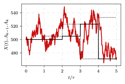
Figure 1: An example of interaction between the evolution of the system state $X\left(t\right)$ (depicted by the red curve), the last announced poll outcome $A_{k-1}$ (solid black curve), and the most recent conducted poll outcome $A_{k}$ (dotted black curve). Simulation parameters: $\varepsilon_{0}=\varepsilon_{1}=2$, $\tau=5\cdot 10^{-3}$, $N=10^{3}$, $A_{-1}=A_{0}=X\left(0\right)=500$.

Notably, upon closer examination of Fig. 1, there are indications of periodic oscillations arising due to the periodic polling mechanism, even though the initial condition, $A_{-1}=A_{0}=X\left(0\right)$, initially suppresses them. We will explore this effect in a more detail in a subsequent section.

3 Simulation methods

Model driven by the rates (2) could be simulated using one-step transition probability approach [48], with the condition that the time step is smaller than $\tau$ and the ratio between $\tau$ and the time step is an integer. The issue with this approach in the general case is that it is slow and it generates biased samples [49]. Gillespie method [49] could be employed as an approximation, but it would inaccurately represent one transition per every polling period, specifically the transition during which the crossover to the next polling period occurs. While the potential error is likely negligible, as misrepresentation becomes more noticeable only for small values of $\tau$, but the delay effect induced by the polling mechanism is also smaller for smaller $\tau$ as well. Typically, for systems with delays a modified next reaction method is used [49]. In our case, this method has performed approximately $4$ times slower than the Gillespie method, but still, it has an advantage over the Gillespie method as it produces time series without misrepresenting any transition. In this section, we will discuss our adaptation of the Gillespie method for systems with delays, as well as introduce a macroscopic simulation method developed specifically for this model. We will also briefly touch upon formalizing the model as a one-dimensional Markov chain.

3.1 Adapted Gillespie method for periodic polling with announcement delays

We propose the adapted Gillespie method by combining the best features of the Gillespie method and the next reaction method. Our adaption, outline given in Algorithm 1, is based on the Gillespie method, but introduces delay $\tau$, the poll index $k$, and the $k$-th poll outcome $A_{k}$. In Step 5 of the algorithm, the delay mechanism is introduced by building on the idea of the internal reaction clock $R$ from the next reaction method. This allows recalculation of the transition rates according to updated recent poll outcomes. The conditional statement in Step 5 of the algorithm checks if a poll should be conducted before the next transition (reaction, in the language of the original next reaction method). The while loop is used to handle an edge case when more than a single poll falls between $2$ transitions. This edges arises often when $\tau\apprle\frac{1}{N^{2}}$.

Algorithm 1 Adapted Gillespie method

1. Set parameter values $\varepsilon_{0}$, $\varepsilon_{1}$, $N$, $\tau$. Set desired initial conditions $A_{-1}$, $X\left(0\right)$. Set the clock $t=0$. Set the current polling period index $k=0$. Conduct the initial poll, $A_{0}=X\left(0\right)$.

2. Calculate the system-wide transition rates $\lambda^{+}$ and $\lambda^{-}$ according to Eq. (2).

3. Calculate total transition rate $\lambda^{T}=\lambda^{+}+\lambda^{-}$.

4. Sample the time until the next reaction from an exponential distribution, $\Delta t\sim\text{Exp}\left(\lambda^{T}\right)$.

5. While $t+\Delta t\geq\left(k+1\right)\tau$:

   • Increment the polling period index $k\rightarrow k+1$.

   • Conduct the $k$-th poll, $A_{k}=X\left(t\right)$.

   • Calculate the remaining time until the next reaction (according to the internal reaction clock) $R=\lambda^{T}\left[t+\Delta t-k\tau\right]$.

   • Update $\lambda^{+}$, $\lambda^{-}$ according to Eq. (2). Update $\lambda^{T}$ accordingly.

   • Adjust the time until the next reaction $\Delta t=\frac{R}{\lambda^{T}}$.

   • Update the clock $t\rightarrow k\tau$

6. Sample uniformly distributed random value $r\sim\mathcal{U}\left(0,\lambda^{T}\right)$. If $r\leq\lambda^{+}$, set $X\left(t+\Delta t\right)=X\left(t\right)+1$. Otherwise set $X\left(t+\Delta t\right)=X\left(t\right)-1$.

7. Update the clock $t\rightarrow t+\Delta t$.

8. Go back to Step 4 or end the simulation.

3.2 Macroscopic simulation method

This simulation method relies on the fact that $A_{k-1}$ in (2) remains constant throughout the polling interval. This enables us to introduce the effective individual agent transition rates that remain constant for the duration of the $k$-th polling period:

$$\varepsilon_{1}^{\left(k\right)}=\varepsilon_{1}+A_{k-1},\quad\varepsilon_{0}^{\left(k\right)}=\varepsilon_{0}+\left(N-A_{k-1}\right).$$ (4)

These effective rates encompass both the truly independent transitions and the peer pressure exerted through the last announced poll outcome. It is important to note that the peer pressure exerted this way is similar to the peer pressure exerted by zealots [42, 43, 44, 45, 46], as the peer pressure term involving $A_{k-1}$ will not change with the system state during the $k$-th polling period, although the agents themselves will still change their state. Subsequently, the system-wide transition rates in (2) can be rewritten as:

$$\lambda_{k}^{+}=\left(N-X\right)\varepsilon_{1}^{\left(k\right)},\quad\lambda_{k}^{-}=X\varepsilon_{0}^{\left(k\right)}.$$ (5)

The form of the effective individual agent transition rates suggests that each agent operates independently of others at all times, except when the poll outcome is announced. Upon the announcement of the poll outcome, the transition rates will be updated. Hence, we can approach the analysis of this model from the standpoint of an individual agent, and concentrating only on the current polling period.

In examining the behavior of a single agent, and given that the agent can occupy one of two possible states, the dynamics can be analyzed as a two-state Markov chain. Given the effective individual agent transition rates, Eq. (4), we can formulate the corresponding left stochastic transition matrix governing the transitions of an individual agent over an infinitesimally short time interval $\Delta t$:

$$\boldsymbol{Q}=\left(\begin{array}[]{cc}1-\varepsilon_{0}^{\left(k\right)}\Delta t&\varepsilon_{1}^{\left(k\right)}\Delta t\\ \varepsilon_{0}^{\left(k\right)}\Delta t&1-\varepsilon_{1}^{\left(k\right)}\Delta t\end{array}\right).$$ (6)

By solving the eigenproblem in respect to $\boldsymbol{Q}$, we can infer that the probability to observe an agent in state “$1$” after $m$ steps is given by

$$P_{1}\left(m|P_{1}\left(0\right)\right)=\frac{\varepsilon_{1}^{\left(k\right)}}{\varepsilon_{0}^{\left(k\right)}+\varepsilon_{1}^{\left(k\right)}}+\frac{\varepsilon_{0}^{\left(k\right)}P_{1}\left(0\right)-\varepsilon_{1}^{\left(k\right)}\left[1-P_{1}\left(0\right)\right]}{\varepsilon_{0}^{\left(k\right)}+\varepsilon_{1}^{\left(k\right)}}\left[1-\left(\varepsilon_{0}^{\left(k\right)}+\varepsilon_{1}^{\left(k\right)}\right)\Delta t\right]^{m}.$$ (7)

In the above $P_{1}\left(0\right)$ represents the “initial” condition of the Markov chain describing individual agent dynamics. Typically, $P_{1}\left(0\right)$ assumes a value of $1$ if the agent under consideration is initially in the “$1$” state, or $0$ otherwise. Additionally, it proves convenient to introduce notation $P_{1}\left(\infty\right)$ which denotes the stationary probability of observing the agent in the “$1$” state,

$$P_{1}\left(\infty\right)=\frac{\varepsilon_{1}^{\left(k\right)}}{\varepsilon_{0}^{\left(k\right)}+\varepsilon_{1}^{\left(k\right)}}=\frac{\varepsilon_{1}+A_{k-1}}{\varepsilon_{0}+\varepsilon_{1}+N}.$$ (8)

By taking the continuous time limit, i.e., letting $\Delta t\rightarrow 0$ and $m\rightarrow\infty$ (with $s=m\Delta t=\text{const}$), we obtain the conditional probability to observe an agent in the “$1$” state after time span $s$,

$$P_{1}\left(s|P_{1}\left(0\right)\right)=P_{1}\left(\infty\right)+\left[P_{1}\left(0\right)-P_{1}\left(\infty\right)\right]\exp\left[-\left(\varepsilon_{0}^{\left(k\right)}+\varepsilon_{1}^{\left(k\right)}\right)s\right].$$ (9)

We can use Eq. (9) to simulate the behavior of all $N$ agents without resorting to the time-consuming direct simulation of the noisy voter model with periodic polling mechanism. Let $X\left(t\right)$ denote the system state at some arbitrary time $t$, and let $s$ be a positive time increment such that $k\tau\leq t<t+s\leq\left(k+1\right)\tau$. Then, $X\left(t+s\right)$ can be sampled by adding two binomial random variables

$$X\left(t+s\right)=B_{1\rightarrow 1}\left[X\left(t\right),P_{1}\left(s|1\right)\right]+B_{0\rightarrow 1}\left[N-X\left(t\right),P_{1}\left(s|0\right)\right].$$ (10)

In the expression above, $B_{1\rightarrow 1}\left[\ldots\right]$ corresponds to the count of agents that were in state “$1$” at time $t$ and ended up in state “$1$” at time $t+s$. These agents may have remained in state “$1$” for the duration $s$, or they might have exited and subsequently returned to state “$1$”. In this setup, the specific evolution of an individual agent’s state doesn’t influence the outcome; only the initial and final states matter. Given there were $X\left(t\right)$ agents in state “$1$” at time $t$, and the probability that an agent starting in state “$1$” will end up in state “$1$” is given by $P_{1}\left(s|1\right)$, then $B_{1\rightarrow 1}\left[\ldots\right]$ is an outcome of $X\left(t\right)$ Bernoulli trials with a success probability of $P_{1}\left(s|1\right)$. Similarly, $B_{0\rightarrow 1}\left[\ldots\right]$ is an outcome of $N-X\left(t\right)$ Bernoulli trials with a success probability of $P_{1}\left(s|0\right)$.

This approach is most efficient when $t=k\tau$ and $s=\tau$, although finer-scale simulations are also possible for $s<\tau$. As long as the sampling period $s$ encompasses a large number of transitions, this method proves to be more efficient than a direct simulation without compromising quality of the sampled time series. The detailed outline of the macroscopic simulation method is provided in Algorithm 2.

Algorithm 2 Macroscopic simulation method

1. Set parameter values $\varepsilon_{0}$, $\varepsilon_{1}$, $N$, $\tau$. Set desired initial conditions $A_{-1}$, $X\left(0\right)$. Set desired sampling period $s$ (note that $\tau/s$ must be a positive integer). Set the clock $t=0$. Set the current polling period index $k=0$.

2. Calculate the effective transition rates $\varepsilon_{0}^{\left(k\right)}=\varepsilon_{0}+\left(N-A_{k-1}\right)$, $\varepsilon_{1}^{\left(k\right)}=\varepsilon_{1}+A_{k-1}$.

3. Calculate the transition probabilities $P_{1}\left(s|1\right)$ and $P_{1}\left(s|0\right)$.

4. Conduct the $k$-th poll, $A_{k}=X\left(t\right)$.

5. Sample binomial random values $B_{1\rightarrow 1}\sim\text{Binom}\left[X\left(t\right),P_{1}\left(s|1\right)\right]$, $B_{0\rightarrow 1}\sim\text{Binom}\left[N-X\left(t\right),P_{1}\left(s|0\right)\right]$.

6. Update the system state $X\left(t+s\right)=B_{1\rightarrow 1}+B_{0\rightarrow 1}$.

7. Update the clock $t\rightarrow t+s$.

8. If $t<\left(k+1\right)\tau$, go back to Step 5.

9. Increment the polling period index $k\rightarrow k+1$.

10. Go back to Step 2 or end the simulation.

3.3 Comparison of the Monte-Carlo simulation algorithms

Both of the methods discussed earlier are Monte Carlo simulation algorithms. In order to obtain the temporal dependence of statistical moments or the stationary distribution, it is necessary to conduct multiple simulations with the same parameter set and subsequently average over the ensemble. Comparing the results obtained from simulations using these methods allows us to verify the validity of the macroscopic simulation method, which may not be immediately evident.

In the different simulations shown in Fig. 2 we keep $N$ fixed and equal to $10^{3}$, systematically vary the values of $\varepsilon_{i}$ and $\tau$ parameters, while initial conditions are purposefully selected to be very different. Nevertheless in all cases the results of numerical simulations from both models match reasonably well. So well that we are forced to make the red $\left\langle X\left(t\right)\right\rangle$ curve (obtained with the macroscopic simulation method) thicker. Fig. 2 (a) and (b) show how the mean and variance evolve for the base parameter set. The selected value of $\tau=10^{-2}$ appears to be sufficient for the statistical moments to converge towards their stationary values; the mean approaches $A_{-1}$. As the delay $\tau$ is kept the same in Fig. 2 (c) and (d), the statistical moments still converge to their respective stationary values. In Fig. 2 (d) we can clearly observe localization phenomenon as the ensemble variance temporarily increases before converging to the stationary value. From Fig. 2 (e)-(h) it is evident that for shorter delay, $\tau=10^{-3}$, the statistical moments fail to converge their respective stationary values: instead some intermediate values are reached. From Fig. 2 it is not clear what impact $\varepsilon_{i}$ parameters have, while the initial conditions appear to be extremely important. This was expected as the macroscopic simulation method takes the effective rates as its input.

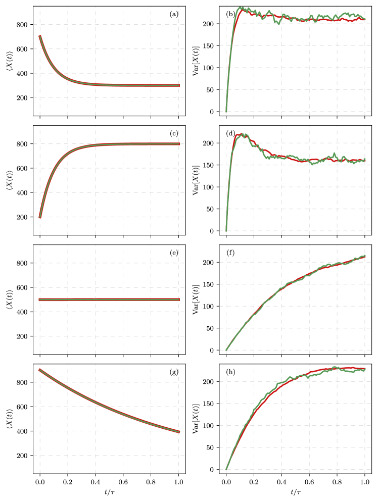
Figure 2: The evolution of statistical moments, mean ((a), (c), (e) and (g)) and variance ((b), (d), (f) and (h)), of numerically simulated ensembles. Different curves correspond to results obtained from the two simulation methods: red curve corresponds to the macroscopic simulation method (with ensemble size of $10^{4}$), green dashed curve corresponds to the adapted Gillespie method (with ensemble size of $10^{3}$). Different pairs of subfigures were obtained with the different parameter sets: $\varepsilon_{0}=\varepsilon_{1}=0.5$, $\tau=10^{-2}$, $A_{-1}=300$ and $A_{0}=X\left(0\right)=700$ ((a) and (b)); $\varepsilon_{0}=\varepsilon_{1}=2$, $\tau=10^{-2}$, $A_{-1}=800$ and $A_{0}=X\left(0\right)=200$ ((c) and (d)); $\varepsilon_{0}=0.5$, $\varepsilon_{1}=0.5$, $\tau=10^{-3}$ and $A_{-1}=A_{0}=X\left(0\right)=500$ ((e) and (f)); $\varepsilon_{0}=\varepsilon_{1}=2$, $\tau=10^{-3}$, $A_{-1}=100$ and $A_{0}=X\left(0\right)=900$ ((g) and (h)). Shared parameter values: $N=10^{3}$.

Producing Fig. 2 allows us to at least approximately compare the speed of the methods. It took couple of seconds to obtain all of the results using the macroscopic simulation method, while it took couple of minutes using the adapted Gillespie method. Given difference in the ensemble sizes, macroscopic simulation method produces the results roughly $10^{2}$ times faster for the considered parameter sets and the selected time resolution. The difference in favor of the macroscopic simulation method was expected as it doesn’t simulate individual transitions, only $X\left(t\right)$ values for desired $t$.

In the subsequent sections, we present the results obtained by simulating large a number of polling periods. Wherever feasible, we will use both simulation methods to reinforce validity of our results and to further validate the equivalence of both methods.

3.4 Semi-analytical approach based on the transition matrix for poll outcomes

If we focus only on the poll outcomes $A_{i}$, then the model under consideration reduces to the second-order Markov chain as the distribution of $A_{i}$ depends on $A_{i-1}$ and $A_{i-2}$. For finite $N$ the phase space of the model is finite, for this reason we can reduce the second-order Markov chain to the first-order Markov chain. Let us derive an expression for the left stochastic transition matrix elements of this first-order Markov chain.

If we focus solely on the poll outcomes $A_{i}$, the model can be treated as a second-order Markov chain, as the distribution of $A_{i}$ is conditioned on both $A_{i-1}$ and $A_{i-2}$. In the case of a finite $N$, the phase space of the model is also finite. Consequently, we have the ability to further reduce the second-order Markov chain into a first-order Markov chain. Let us proceed to derive an expression for the left stochastic transition matrix elements of this first-order Markov chain.

Upon reducing the second-order Markov chain, we effectively introduce two-dimensional system state $\left(A_{i},A_{i-1}\right)$. As $A_{i}\in\left[0,N\right]$, we can uniquely map the two-dimensional system state into one-dimensional index $K_{i}$:

$$K_{i}=1+A_{i}+\left(N+1\right)\cdot A_{i-1}.$$ (11)

Index $K_{i}$ corresponds to the row or column indices of the transition matrix $\boldsymbol{T}$. Given that $A_{i}\in\left[0,N\right]$, we have that $K_{i}\in\left[1,\left(N+1\right)^{2}\right]$. This implies that the transition matrix will have $\left(N+1\right)^{4}$ elements, although only $\left(N+1\right)^{2}$ of them will be non-zero. The one-dimensional index $K_{i}$ also uniquely maps to the two-dimensional system state $\left(A_{i},A_{i-1}\right)$:

$$A_{i}=K_{i}-1-\left(N+1\right)\left\lfloor\frac{K_{i}-1}{N+1}\right\rfloor,\qquad A_{i-1}=\left\lfloor\frac{K_{i}-1}{N+1}\right\rfloor.$$ (12)

In the indexing scheme introduced above, the $\left(K,M\right)$ element of the left stochastic transition matrix $\boldsymbol{T}$ representing $M\rightarrow K$ transition is given by

$$T_{K,M} =P\left[M\rightarrow K\right]=$$

$$=P\left[\left(M-1-\left(N+1\right)\left\lfloor\frac{M-1}{N+1}\right\rfloor,\left\lfloor\frac{M-1}{N+1}\right\rfloor\right)\rightarrow\left(K-1-\left(N+1\right)\left\lfloor\frac{K-1}{N+1}\right\rfloor,\left\lfloor\frac{K-1}{N+1}\right\rfloor\right)\right]=$$

$$=\begin{cases}P\left[K-1-\left(N+1\right)\left\lfloor\frac{K-1}{N+1}\right\rfloor|\left\lfloor\frac{K-1}{N+1}\right\rfloor,\left\lfloor\frac{M-1}{N+1}\right\rfloor,\tau\right]&\text{if }\left\lfloor\frac{K-1}{N+1}\right\rfloor=M-1-\left(N+1\right)\left\lfloor\frac{M-1}{N+1}\right\rfloor,\\ 0&\text{otherwise.}\end{cases}$$ (13)

The conditional probability in the above is given by

$$P\left[A_{i+1}|A_{i},A_{i-1},\tau\right]=\sum_{k=0}^{A_{i+1}}p_{\text{Binom}}\left[k,A_{i},P_{1}\left(\tau|1,A_{i-1}\right)\right]\cdot p_{\text{Binom}}\left[A_{i+1}-k,N-A_{i},P_{1}\left(\tau|0,A_{i-1}\right)\right].$$ (14)

In the above, $p_{\text{Binom}}\left(k,N,p\right)$ represents the probability mass function of the Binomial distribution with $N$ trials and success probability $p$, while $P_{1}\left(\ldots\right)$ corresponds to Eq. (9) additionally conditioned that the last announced poll outcome was $A_{i-1}$. The last announced poll outcome is not explicitly present in Eq. (9); however, it is implicitly present as a part of $P_{1}\left(\infty\right)$ and $\varepsilon_{i}^{\left(k\right)}$.

This approach provides an alternative semi-analytical method for simulating the model. The primary drawback of this method is that it is very time consuming, making it feasible only for small $N$. However, solving the eigenproblem with respect to $\boldsymbol{T}$ allows obtaining the exact stationary distribution or the entire temporal evolution of the distribution for the selected parameters. The methods discussed earlier are faster, but they do not yield exact results.

4 Stationary poll outcome distributions

As previously discussed the outcome of the next poll $A_{k+1}$ for an arbitrary polling interval $\tau$ depends on the last announced poll outcome $A_{k-1}$ and the system state at the start of the polling period $X\left(k\tau\right)$, which corresponds to $A_{k}$. Consequently, the model behaves as a second-order Markov chain. As was discussed in the previous section, it can be reduced to the first-order Markov chain. Determining eigenvectors and eigenvalues of the associated transition matrix yields the temporal evolution of the poll outcome distribution and also the exact stationary poll outcome distribution. However, the analytical solution of this eigenproblem is elusive, necessitating a numerical approach. Due to the time-consuming nature of the numerical solution of the eigenproblem, it is only practical for small $N$. Although we are unable to obtain analytical results for arbitrary $\tau$ and $N$, we can gain some insights about the poll outcome distributions by considering extremely small or large $\tau$.

4.1 Analytical consideration of the small $\tau$ limit

For small values of $\tau$, i.e., $\tau\ll\frac{1}{X\varepsilon_{0}^{\left(k\right)}+\left(N-X\right)\varepsilon_{1}^{\left(k\right)}}\approx\frac{2}{N\left(\varepsilon_{0}+\varepsilon_{1}+N\right)}$, when few or no transitions occur during the polling period, the impact of the information delay induced by the polling mechanism is negligible, because polling information is updated almost as frequently as the system state is. Consequently, in this limit, the model is almost equivalent to the noisy voter model. This implies that the poll outcomes should be distributed according to a Beta-binomial distribution, sharing the same distribution parameter values expected from the noisy voter model, i.e., $A_{\infty}\sim\text{BetaBin}\left(N,\varepsilon_{1},\varepsilon_{0}\right)$. In Fig. 3, it is evident that the theoretical prediction aligns well with the results from numerical simulations.

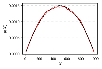
Figure 3: Stationary poll outcome distribution of the model with small $\tau$. The probability mass function obtained from the numerical simulations is shown as a red curve (snapshot taken after $10^{8}$ polls), while dashed black curve corresponds to the probability mass function of the BetaBin$\left(N,\varepsilon_{1},\varepsilon_{0}\right)$. Simulation parameters: $\varepsilon_{0}=\varepsilon_{1}=2$, $\tau=10^{-7}$, $N=10^{3}$.

4.2 Analytical consideration of the large $\tau$ limit

Utilizing insights obtained in Section 3.2, we can explore the statistical characteristics of the model in the limit of large $\tau$. Let us consider $\tau$ to be large if both $P_{1}\left(\tau|0\right)$ and $P_{1}\left(\tau|1\right)$ are close to $P_{1}\left(\infty\right)$. Closer inspection of Eq. (9) suggests that to be considered large $\tau$ has to satisfy $\tau\gg\frac{1}{\varepsilon_{0}^{\left(k\right)}+\varepsilon_{1}^{\left(k\right)}}=\frac{1}{\varepsilon_{0}+\varepsilon_{1}+N}$. For $\tau$ this large a substantial number of transitions occur during a single polling period. Consequently, for large $\tau$, the next poll outcome $A_{k+1}$ depends only on $A_{k-1}$, which is implicitly embedded in $P_{1}\left(\infty\right)$ through the $\varepsilon_{i}^{\left(k\right)}$ values. This means that the model can now be analyzed not as a second-order Markov chain, but instead as two independent first-order Markov chains: one for polls with even indices and another for polls with odd indices. These two Markov chains are identical in all senses except for their initial conditions. As this case is not as trivial as extremely small $\tau$ case, let us examine this case more carefully.

Let $p_{\mathcal{T}}\left(x|u\right)$ denote the probability of observing $A_{i+1}=x$ given that $A_{i-1}=u$, i.e., the transition probability between the outcomes of subsequent even or odd polls. The distribution of the $i$-th poll outcome can be obtained through a recursive relationship

$$p_{i+1}\left(x\right)=\sum_{u=0}^{N}p_{\mathcal{T}}\left(x|u\right)p_{i-1}\left(u\right),$$ (15)

with the initial conditions

$$p_{0}\left(x\right)=\delta\left(x-A_{0}\right),\quad p_{-1}\left(x\right)=\delta\left(x-A_{-1}\right).$$ (16)

In the expression above, $\delta\left(x\right)$ denotes a Kronecker delta function, its value is $1$ if $x=0$ and is $0$ otherwise. If both $P_{1}\left(\tau|0\right)$ and $P_{1}\left(\tau|1\right)$ are close to $P_{1}\left(\infty\right)$, then $p_{\mathcal{T}}\left(x|u\right)$ corresponds to a Binomial distribution probability mass function with $N$ trials and the success probability $P_{1}\left(\infty\right)$, which is implicitly a function of $u$ Eq. (8). Obtaining a general analytical expressions for $p_{i}\left(x\right)$ or $p_{\infty}\left(x\right)$ doesn’t seem feasible, but this problem could be approached from a numerical perspective. Approach discussed in Section (3.4) would yield similar results to iterating Eq. (15), but the approach discussed in Section (3.4) is applicable for broad range $\tau$ values. Instead let us focus on deriving expressions for the evolution of statistical moments, mean and variance, of the poll outcome distribution.

As the poll outcome distributions are linked via recursive relationship, Eq. (15), we can show that the mean will satisfy another recursive relationship

$$\left\langle A_{i+1}\right\rangle =\sum_{x=0}^{N}xp_{i+1}\left(x\right)=\sum_{u=0}^{N}\left[\left(\sum_{x=0}^{N}xp_{\mathcal{T}}\left(x|u\right)\right)p_{i-1}\left(u\right)\right]=$$

$$=\sum_{u=0}^{N}\frac{N\left(\varepsilon_{1}+u\right)}{\varepsilon_{0}+\varepsilon_{1}+N}p_{i-1}\left(u\right)=\frac{N\left(\varepsilon_{1}+\left\langle A_{i-1}\right\rangle\right)}{\varepsilon_{0}+\varepsilon_{1}+N}.$$ (17)

This recursive form can be rewritten as

$$\left\langle A_{k}\right\rangle=A_{\infty}+\left(A_{0}-A_{\infty}\right)\left(\frac{N}{\varepsilon_{0}+\varepsilon_{1}+N}\right)^{k/2},$$ (18)

where $k$ is the poll index, and $A_{\infty}$ is the stationary value of the mean,

$$A_{\infty}=\frac{N\varepsilon_{1}}{\varepsilon_{0}+\varepsilon_{1}}.$$ (19)

Notably, the stationary mean bears an identical form to the mean of the Beta-binomial distribution with $N$ number of trials and the shape parameters equal to $m\varepsilon_{i}$ (with $m$ being a positive real number). Repeating the same derivation for the odd poll indices $k$, we obtain

$$\left\langle A_{k}\right\rangle=A_{\infty}+\left(A_{-1}-A_{\infty}\right)\left(\frac{N}{\varepsilon_{0}+\varepsilon_{1}+N}\right)^{\left(k+1\right)/2}.$$ (20)

The recursive relationship for the second raw moment is somewhat more complicated

$$\left\langle A_{i+1}^{2}\right\rangle =\sum_{x=0}^{N}x^{2}p_{i+1}\left(x\right)=\sum_{u=0}^{N}\left[\left(\sum_{x=0}^{N}x^{2}p_{\mathcal{T}}\left(x|u\right)\right)p_{i-1}\left(u\right)\right]=$$

$$=\frac{N\left[\varepsilon_{1}\left(\varepsilon_{0}+N+\varepsilon_{1}N\right)+\left(\varepsilon_{0}-\varepsilon_{1}+N+2\varepsilon_{1}N\right)\left\langle A_{i-1}\right\rangle+\left(N-1\right)\left\langle A_{i-1}^{2}\right\rangle\right]}{\left(\varepsilon_{0}+\varepsilon_{1}+N\right)^{2}}.$$ (21)

This recursive form can be rewritten as

$$\left\langle A_{k}^{2}\right\rangle=A_{\infty}^{\left(2\right)}+\left[A_{0}^{2}-A_{\infty}^{\left(2\right)}-A_{\text{mid}}^{\left(2\right)}\right]\left[\frac{N\left(N-1\right)}{\left(\varepsilon_{0}+\varepsilon_{1}+N\right)^{2}}\right]^{k/2}+A_{\text{mid}}^{\left(2\right)}\left[\frac{N}{\varepsilon_{0}+\varepsilon_{1}+N}\right]^{k/2},$$ (22)

with

$$A_{\text{mid}}^{\left(2\right)} =\left(A_{0}-A_{\infty}\right)\frac{\varepsilon_{0}-\varepsilon_{1}+N+2\varepsilon_{1}N}{\varepsilon_{0}+\varepsilon_{1}+1},$$ (23)

$$A_{\infty}^{\left(2\right)} =\left\langle A_{\infty}^{2}\right\rangle=\frac{N\varepsilon_{1}\left[\left(\varepsilon_{0}+N+\varepsilon_{1}N\right)\left(\varepsilon_{0}+\varepsilon_{1}\right)+\left(\varepsilon_{0}-\varepsilon_{1}+N+2\varepsilon_{1}N\right)N\right]}{\left(\varepsilon_{0}+\varepsilon_{1}\right)\left[\left(\varepsilon_{0}+\varepsilon_{1}+N\right)^{2}-N\left(N-1\right)\right]}.$$ (24)

Given the expression for the second raw moment, the variance can be shown to be

$$\text{Var}\left[A_{k}\right]= \left\langle A_{k}^{2}\right\rangle-\left\langle A_{k}\right\rangle^{2}=\text{Var}\left[A_{\infty}\right]+\left(A_{0}^{2}-A_{\infty}^{\left(2\right)}-A_{\text{mid}}^{\left(2\right)}\right)\left[\frac{N\left(N-1\right)}{\left(\varepsilon_{0}+\varepsilon_{1}+N\right)^{2}}\right]^{k/2}+$$

$$+\left[A_{\text{mid}}^{\left(2\right)}-2A_{\infty}\left(A_{0}-A_{\infty}\right)\right]\left(\frac{N}{\varepsilon_{0}+\varepsilon_{1}+N}\right)^{k/2}-\left(A_{0}-A_{\infty}\right)^{2}\left(\frac{N}{\varepsilon_{0}+\varepsilon_{1}+N}\right)^{2k}.$$ (25)

Repeating the same derivation the variance for the odd poll indices $k$, we obtain

$$\text{Var}\left[A_{k}\right]= \text{Var}\left[A_{\infty}\right]+\left(A_{-1}^{2}-A_{\infty}^{\left(2\right)}-A_{\text{mid}}^{\left(2\right)}\right)\left[\frac{N\left(N-1\right)}{\left(\varepsilon_{0}+\varepsilon_{1}+N\right)^{2}}\right]^{\left(k+1\right)/2}+$$

$$+\left[A_{\text{mid}}^{\left(2\right)}-2A_{\infty}\left(A_{-1}-A_{\infty}\right)\right]\left(\frac{N}{\varepsilon_{0}+\varepsilon_{1}+N}\right)^{\left(k+1\right)/2}-\left(A_{-1}-A_{\infty}\right)^{2}\left(\frac{N}{\varepsilon_{0}+\varepsilon_{1}+N}\right)^{2k+2}.$$ (26)

In the expressions for both even and odd $k$, $\text{Var}\left[A_{\infty}\right]$ stands for the stationary value of the variance,

$$\text{Var}\left[A_{\infty}\right]=\frac{N\varepsilon_{1}\varepsilon_{0}\left(\varepsilon_{0}+\varepsilon_{1}+N\right)^{2}}{\left(\varepsilon_{0}+\varepsilon_{1}\right)^{2}\left[\left(\varepsilon_{0}+\varepsilon_{1}\right)^{2}+\left(2\varepsilon_{0}+2\varepsilon_{1}+1\right)N\right]}.$$ (27)

For the large number of agents $N\gg\left(\varepsilon_{0}+\varepsilon_{1}\right)$, the stationary value of the variance can be approximated by

$$\text{Var}\left[A_{\infty}\right]\approx\frac{\varepsilon_{1}\varepsilon_{0}N^{2}}{\left(\varepsilon_{0}+\varepsilon_{1}\right)^{2}\left(2\varepsilon_{0}+2\varepsilon_{1}+1\right)}.$$ (28)

This approximation of the stationary variance has the same form as the variance of the Beta-binomial distribution with $N$ number of trials, and the shape parameters equal to $2\varepsilon_{i}$.

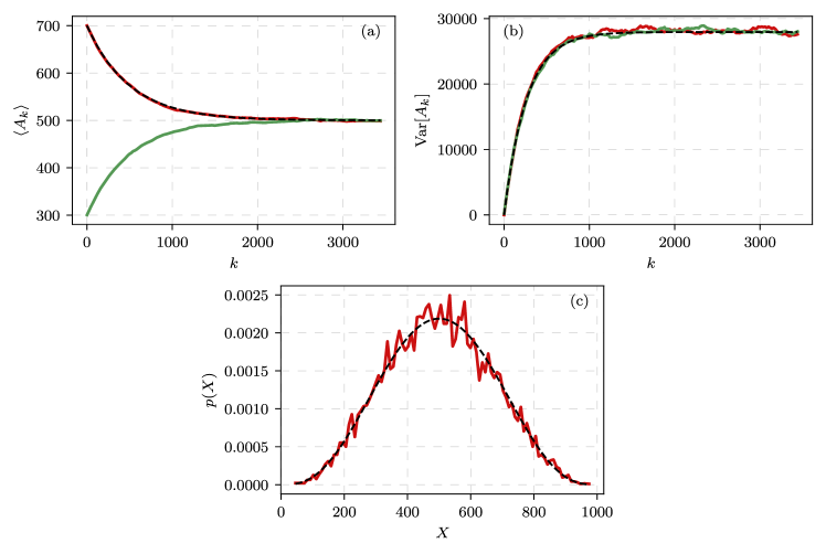
Figure 4: The evolution of the statistical moments, mean (a) and variance (b), as well as the stationary distribution (c) of the model with large $\tau$. In (a) and (b) red curve shows the evolution of the respective statistical moment for the polls with even indices, green curve represents polls with odd indices, while dashed black curve shows the analytical prediction, Eq. (18) for (a), Eq. (25) for (b), and the probability mass function of $\text{BetaBin}\left(N,2\varepsilon_{1},2\varepsilon_{0}\right)$ for (c). Simulation parameters: $\varepsilon_{0}=\varepsilon_{1}=2$, $N=10^{3}$, $\tau=0.03$, $A_{-1}=300$, and $A_{0}=X\left(0\right)=700$.

The derivation above implies that, at least for large $\tau$, the model is effectively driven by two identical and independent processes. The form of Eqs. (19) and (28) suggest that these processes could be equivalent to the standard noisy voter model, but it is not a definite proof. In Fig. 4 (a) and (b), numerical simulation results are shown, providing a comparison between the evolution of the ensemble’s statistical moments and the theoretical predictions derived from Eqs. (18) and (25). The theoretical predictions match the results from numerical simulations reasonably well. Furthermore in Fig. 4 (c) it can be seen that the stationary probability mass function is fitted rather well by the probability mass function of $\text{BetaBin}\left(N,2\varepsilon_{1},2\varepsilon_{0}\right)$.

4.3 Numerical analysis of the intermediate $\tau$ range

For the intermediate $\tau$ and large $N$, deriving a general analytical expression for the stationary distribution or its statistical moments is not feasible. From the previous discussion, we have seen that Beta-binomial distribution is a good approximation of the stationary poll outcome distribution for small and large $\tau$. Let us assume that this approximation remains valid for the intermediate $\tau$ as well. However, we expect that the shape parameters of the approximating Beta-binomial distribution, denoted as $\hat{\alpha}$ and $\hat{\beta}$, may vary with $\tau$. We investigate this relationship by conducting a series of numerical simulations.

Fig. 5 was produced by numerical simulation of the symmetric case with $\varepsilon_{0}=\varepsilon_{1}=\varepsilon=2$ and $N=10^{3}$ using the adapted Gillespie method (green curve) and the macroscopic simulation method (red curve). Consistent with the expectations for the symmetric case, the numerical simulations yield almost identical dependence of $\hat{\alpha}$ and $\hat{\beta}$ on $\tau$. For this reason only $\hat{\alpha}$ dependence on $\tau$ is shown in Fig. 5. For small and large $\tau$, we reliably recover predictions made earlier in this section. Specifically, in the limit of small $\tau$, we observe that $\hat{\alpha}\approx\hat{\beta}\approx\varepsilon=2$, and in the limit of large $\tau$, we observe that $\hat{\alpha}\approx\hat{\beta}\approx 2\varepsilon=4$. Remarkably, the dependence for the intermediate $\tau$ is not a sigmoid function interpolating between the limiting cases. Instead, for some intermediate value of $\tau$ a peak in $\hat{\alpha}$ is observed. Notably, the observed peak in the scaling behavior implies that for some intermediate $\tau$ the fluctuations around the mean experience even stronger damping than in the large $\tau$ limit.

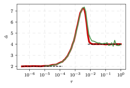
Figure 5: Scaling behavior of the shape parameter estimate $\hat{\alpha}$ in respect to the polling period $\tau$. Different solid curves correspond to results obtained from the two simulation methods: red curve corresponds to the macroscopic simulation method and green curve corresponds to the adapted Gillespie method. Dashed black lines show theoretical predictions for small and large $\tau$. Simulation parameters: $\varepsilon_{0}=\varepsilon_{1}=\varepsilon=2$ and $N=10^{3}$.

By considering a smaller value of $N$, the dependence between $\hat{\alpha}$ and $\tau$ can also be obtained from the semi-analytical approach discussed in Section 3.4. In Fig. 6, the results obtained from the semi-analytical approach match with those from purely numerical simulations. This agreement allows us to conclude that the observed peak is a characteristic of the model and not an artifact caused by the chosen numerical simulation method. Additionally, it can be seen that the range of $\tau$ values for which the peak was observed has shifted, which is expected since the definition of what constitutes small and large $\tau$ depends on $N$. The peak value of $\hat{\alpha}$ has also decreased, likely because the smaller the number of agents the more frequent truly independent transition are, and there are less transitions caused by the peer pressure exerted through the poll outcomes.

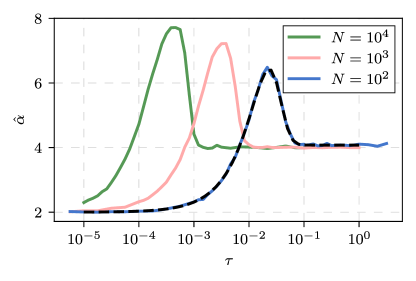
Figure 6: Scaling behavior of the shape parameter estimate $\hat{\alpha}$ in respect to the polling period $\tau$ when number of agents $N$ varies. Solid curves were obtained by numerical simulation, while dashed black curve was obtained by semi-analytical method discussed in Section 3.4. Solid pale red curve is the same as the red curve in Fig. 5. Simulation parameters: $\varepsilon_{0}=\varepsilon_{1}=\varepsilon=2$ (in all cases) and $N=10^{2}$ (blue and dashed black curves), $10^{3}$ (pale red curve) and $10^{4}$ (green curve) .

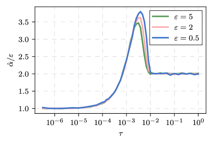
Figure 7: Scaling behavior of the normalized shape parameter estimate $\hat{\alpha}/\varepsilon$ in respect to the polling period $\tau$ when independent transition rates $\varepsilon$ vary. Pale red curve is the same as the red curve in Fig. 5. Simulation parameters: $\varepsilon_{0}=\varepsilon_{1}=\varepsilon=5$ (blue curve), $2$ (pale red curve) and $0.5$ (green curve), $N=10^{3}$ (in all cases).

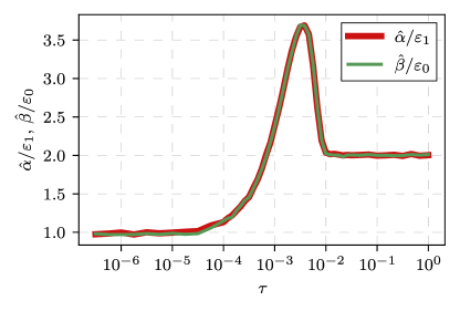
Figure 8: Scaling behavior of the normalized shape parameter estimates $\hat{\alpha}/\varepsilon_{1}$, $\hat{\beta}/\varepsilon_{0}$ in respect to the polling period $\tau$ with asymmetric independent transition rates. Simulation parameters: $\varepsilon_{0}=2$, $\varepsilon_{1}=0.5$, $N=10^{3}$.

The peak value of $\hat{\alpha}$ also decreases as the independent transition rates, $\varepsilon_{0}=\varepsilon_{1}=\varepsilon$, increase. Although the location of the peak itself doesn’t seem to change that much, which is expected given that the variation in $\varepsilon$ is less pronounced because $\varepsilon\ll N$ holds. To eliminate the obvious differences between the $\hat{\alpha}$ and $\tau$ dependencies for different $\varepsilon$, we have normalized the shape parameter as $\frac{\hat{\alpha}}{\varepsilon}$. For the normalized shape parameter it is evident that the height of the peak and its exact location varies with non-trivially with $\varepsilon$.

All previously discussed simulations were conducted with symmetric independent transition rates, $\varepsilon_{0}=\varepsilon_{1}=\varepsilon$. If the independent transition rates are asymmetric instead, $\varepsilon_{0}\neq\varepsilon_{1}$, then the shape parameter estimates will reflect this asymmetry. If the shape parameter estimates are appropriately normalized, i.e., $\hat{\alpha}/\varepsilon_{1}$ and $\hat{\beta}/\varepsilon_{0}$, then the asymmetry is eliminated and the scaling curves of the both normalized shape parameter estimates closely mirror each other (see Fig.  10).

4.4 Estimating the $\tau$ range for which anomalous fluctuation damping behavior is observed

From Eq. (10) with $t=k\tau$ and $s\leq\tau$, it is trivial to show that

$$\left\langle X\left(t+s\right)\right\rangle=\frac{\varepsilon_{1}^{\left(k\right)}N+\left[\varepsilon_{0}^{\left(k\right)}X\left(t\right)-\varepsilon_{1}^{\left(k\right)}\left\{N-X\left(t\right)\right\}\right]\exp\left[-\left(\varepsilon_{0}^{\left(k\right)}+\varepsilon_{1}^{\left(k\right)}\right)s\right]}{\varepsilon_{0}^{\left(k\right)}+\varepsilon_{1}^{\left(k\right)}}.$$ (29)

Let us find such $\tau_{c}$ for which $\left\langle X\left(t+\tau_{c}\right)\right\rangle$ is nearly indistinguishable from $\left\langle X\left(\infty\right)\right\rangle$:

$$\left\langle X\left(t+\tau_{c}\right)\right\rangle=\left\langle X\left(\infty\right)\right\rangle\pm\frac{1}{2}.$$ (30)

Solving the above for $\tau_{c}$ yields:

$$\tau_{c}=\frac{\ln\left(2\left|\left\langle X\left(\infty\right)\right\rangle-X\left(0\right)\right|\right)}{\varepsilon_{0}+\varepsilon_{1}+N}.$$ (31)

If we consider the largest possible distance between the initial and stationary states, $\left|\left\langle X\left(\infty\right)\right\rangle-X\left(0\right)\right|=N$, and the smallest $\left|\left\langle X\left(\infty\right)\right\rangle-X\left(0\right)\right|=1$, we obtain:

$$\tau_{c}^{\left(1\right)}=\frac{\ln\left(2N\right)}{\varepsilon_{0}+\varepsilon_{1}+N},\quad\text{and}\quad\tau_{c}^{\left(2\right)}=\frac{\ln\left(2\right)}{\varepsilon_{0}+\varepsilon_{1}+N}.$$ (32)

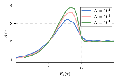
Figure 9: Scaling behavior of the normalized shape parameter estimate $\hat{\alpha}/\varepsilon$ in respect to the normalized polling period $F_{s}\left(\tau\right)$ when number of agents $N$ varies. Solid curves are the same as in Fig. 6.

As can be seen in Fig. 9, anomalous fluctuation damping is observed between these two critical polling periods, i.e., for $\tau_{c}^{\left(2\right)}\apprle\tau\apprle\tau_{c}^{\left(1\right)}$. The numerical simulation results depicted in Fig. 9 mirror those in Fig. 6, with the distinction that the curves obtained by numerical simulation were scaled. It is not necessary to scale the estimated shape parameter values for this figure as all simulations share the same values of independent transition rate, but we still do so for the sake of generality. The scaling function for the polling period, denoted by $F_{s}\left(\tau\right)$, was derived to ensure that, for any given parameter set, $\tau_{c}^{\left(2\right)}=1$ and $\tau_{c}^{\left(1\right)}=C$ (where $C$ could be any real number greater than $1$). The scaling function for the polling period is given by

$$F_{s}\left(\tau\right)=\left[\frac{\varepsilon_{0}+\varepsilon_{1}+N}{\ln\left(2\right)}\cdot\tau\right]^{\frac{\ln\left(C\right)}{\ln\left[\frac{\ln\left(2N\right)}{\ln\left(2\right)}\right]}}.$$ (33)

Expanding on a parallel line of reasoning, one may introduce additional critical polling periods by investigating instances when $\left\langle X\left(t+\tau_{c}\right)\right\rangle$ becomes indistinguishable from $X\left(0\right)$. However, these additional critical polling periods do not provide any addition information. The longer critical polling period obtained this way coincides with $\tau_{c}^{\left(2\right)}$. The shorter critical polling period obtained this way effectively coincides with the small $\tau$ limit taken in Section 4.1.

5 Periodic fluctuations induced by the polling mechanism

Already in Fig. 1 we have observed hints of periodic fluctuations emerging from the noisy voter model with the polling mechanism. In Sections 3.2 and 4.2 we have discussed that the model with the polling mechanism effectively becomes a second-order Markov chain, which also suggests that the model could exhibit periodicity. As can be seen from a few sample trajectories shown in the top subplots of Fig. 10, the larger $\tau$ the more immediately obvious these periodic fluctuations become. Power spectral densities of these time series (see the bottom subplots of Fig. 10) confirm that the main fluctuation frequency is $f=\frac{1}{2\tau}$ in the physical time space, or $f_{k}=\frac{1}{2}$ in the poll index space (here subscript $k$ emphasizes that frequency is given in the poll index space).

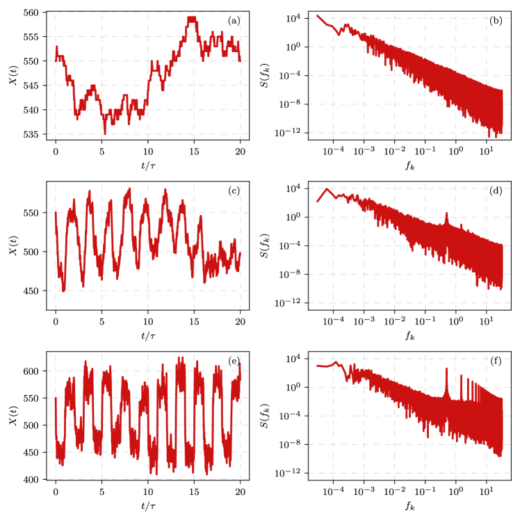
Figure 10: Fragment of time series obtained with different polling periods $\tau$ ((a), (c) and (e)), and the respective power spectral density in the poll index space ((b), (d) and (f)). Simulation parameters: $\varepsilon_{0}=\varepsilon_{1}=2$, $N=10^{3}$, $A_{-1}=450$, $A_{0}=X\left(0\right)=550$ (in all cases), and $\tau=3\cdot 10^{-5}$ ((a) and (b)), $3\cdot 10^{-3}$ ((c) and (d)), and $3\cdot 10^{-2}$ ((e) and (f)).

Emergence of the periodic fluctuations therefore can be quantified by measuring the power spectral density at $f_{k}=\frac{1}{2}$:

$$S\left(f_{k}=\frac{1}{2}\right)=\frac{2}{Mf_{k}^{\left(s\right)}}\left|\sum_{m=0}^{M-1}\tilde{X}\left(\frac{m}{f_{k}^{\left(s\right)}}\tau\right)\cdot\exp\left[-2i\pi\frac{f_{k}}{f_{k}^{\left(s\right)}}m\right]\right|^{2}.$$ (34)

In the above $M$ is the length of the time series, $f_{k}^{\left(s\right)}$ is the sampling frequency in the poll index space (corresponds to the number of samples taken within a single polling period), and $\tilde{X}\left(t\right)$ denotes standardized $X\left(t\right)$, i.e., $\tilde{X}\left(t\right)=\frac{X\left(t\right)-\mu_{X}}{\sigma_{X}}$ (where $\mu_{X}$ is the mean of $X\left(t\right)$ and $\sigma_{X}$ is the standard deviation of $X\left(t\right)$).

Dependence between $S\left(f_{k}=\frac{1}{2}\right)$ and $\tau$ has a trivial sigmoid shape (see Fig. 11). For small $\tau$, the system state manages to update the information in-between the individual transitions, so little change in $S\left(f_{k}=\frac{1}{2}\right)$ is observed as $\tau$ grows slightly larger. If $\tau$ is large, then $\tau$ is already sufficiently large for the system state to reach stationary distribution in-between the polls, and therefore further increase in $\tau$ doesn’t further increase $S\left(f_{k}=\frac{1}{2}\right)$. For intermediate $\tau$, even small increase in $\tau$ allows for larger deviations from the system state at the start of the polling periods, thus causing an increase in periodic fluctuations.

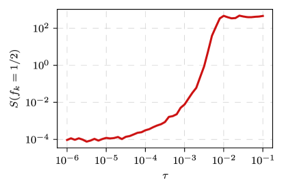
Figure 11: Power spectral density at the frequency corresponding to the observed periodic fluctuations, $S\left(f_{k}=\frac{1}{2}\right)$, of numerically simulated time series with different polling periods $\tau$. Simulation parameters: $\varepsilon_{0}=\varepsilon_{1}=2$, $N=10^{3}$.

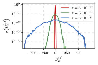
Figure 12: Probability mass function of the differences between the consecutive poll outcomes, $D_{k}^{\left(1\right)}$, with different polling periods $\tau$. Simulated curves are the same as ones shown in Fig. 10.

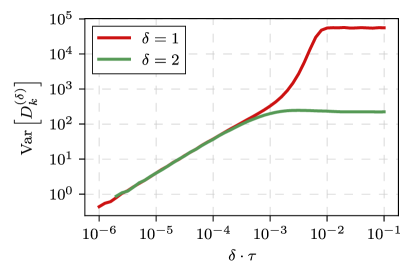
Figure 13: Variance of the differences between the consecutive poll outcomes, $D_{k}^{\left(1\right)}$, and the differences between the next-consecutive poll outcomes, $D_{k}^{\left(2\right)}$, with different polling periods $\tau$. Simulation parameters: $\varepsilon_{0}=\varepsilon_{1}=2$, $N=10^{3}$.

Alternatively, periodic fluctuations could be quantified by looking at the distribution of differences between the consecutive polls:

$$D_{k}^{\left(\delta\right)}=A_{k}-A_{k-\delta}.$$ (35)

For the periodic fluctuations to become apparent the differences between the consecutive poll outcomes, $D_{k}^{\left(1\right)}$, need to become large in comparison to the differences between the next-consecutive poll outcomes, $D_{k}^{\left(2\right)}$. For the sample time series we do indeed observe that the distribution of $D_{k}^{\left(1\right)}$ becomes broader as $\tau$ increases (see Fig. 12). As can be seen in Fig. 13 variance of both $D_{k}^{\left(1\right)}$ and $D_{k}^{\left(2\right)}$ grows with $\tau$, but $D_{k}^{\left(2\right)}$ saturates sooner. Saturation point of $D_{k}^{\left(2\right)}$ roughly coincides with the start of the $\tau$ range for which anomalous damping behavior is observed. Saturation of $D_{k}^{\left(1\right)}$ occurs for larger $\tau$, which roughly corresponds to the end of the $\tau$ range for which anomalous damping behavior is observed.

6 Conclusions

We have examined the implications of information delays arising from the periodic polling mechanism on the opinion formation process. We have achieved this by integrating the periodic polling mechanism into the noisy voter model. Specifically, we replaced the original instantaneous imitative interactions with imitative interactions mediated through periodic polls. Consistent with real-world scenarios, we have assumed a delay in announcing poll outcomes. Additionally, we have also aligned the announcement delay with the polling period. Our findings reveal a non-trivial phenomenology of the generalized model with periodic polling.

Initially, we have adapted the Gillespie method [49] to conduct numerical simulations of the generalized model. When the polling periods are short, this method works reasonably well, but when the polling periods become longer, it becomes slower because each individual agent transition needs to be simulated. By noting that being aware of only the poll outcomes is effectively the same as being influenced by zealot agents (akin to the generalization of the voter model considered in [42, 43, 44, 45]), we were able to propose a macroscopic simulation method, which simulates the outcome of the poll itself. Furthermore, the proposed macroscopic simulation method enables analytical treatment of the model. To verify the results of numerical simulations, we have also discussed how to formulate the eigenproblem for the generalized model and obtain semi-analytical solutions.

Analytical exploration reveals that the generalized model converges to a stationary distribution for both short and long polling periods. In the short polling period limit, the difference between the generalized and the original noisy voter model is minor. Both models converge towards Beta-binomial stationary distribution with shape parameters equal or close to the independent transition rates. In the long polling period limit, the generalized model retains a stationary distribution similar to the Beta-binomial distribution with the shape parameters twice as large as the independent transition rates. This observation implies that the periodic polling mechanism dampens the fluctuations. Numerical simulation for the intermediate polling periods reveals that this damping effect exhibits non-trivial scaling behavior. Notably, for specific intermediate polling periods, the fluctuations are dampened even more than in the long polling period limit. While unable to explain the exact nature of the anomalous damping for the intermediate polling periods, we have identified the range of polling periods for which this anomalous behavior emerges.

The generalized model also displays periodic fluctuations since ordinary differential equations with latency frequently manifest similar behavior. Unlike ordinary differential equations with latency, where initial conditions may initially suppress periodic fluctuations, stochastic perturbations inherent to our model eventually lead to the emergence of periodic fluctuations. Our analysis of the periodic fluctuations in the generalized model is approached from two distinct perspectives. First, we examine the dependence between the polling period and the power spectral density at the relevant frequency. This dependence follows a sigmoid function without displaying any anomalies. Next, we investigate the swings between consecutive polls, denoted as $D_{k}^{\left(1\right)}=A_{k}-A_{k-1}$, and the swings between the second-consecutive polls, denoted as $D_{k}^{\left(2\right)}=A_{k}-A_{k-2}$. The scaling behavior of the variance of these swings differs qualitatively, with major inflection points aligning with the limits of the polling period range where anomalous damping behavior emerges.

In this paper, we have presented a preliminary exploration of the noisy voter model extended with the periodic polling mechanism. The proposed generalization holds promise for further refinement to investigate the demonstrated rich phenomenology more comprehensively. Moreover, it could serve as a foundational framework for analytically probing other variations of latency in noisy voter models. Additionally, this extension may prove instrumental in the development of domain-specific ARCH-like models for opinion dynamics, diverging from traditional applications in finance [50, 51, 52].

Author contributions

AK: Conceptualization, Methodology, Software, Validation, Writing, Visualization. RA: Methodology, Software, Validation, Writing. MR: Conceptualization, Validation, Writing, Supervision. FI: Conceptualization, Writing, Supervision, Project administration.

References

- [1] T. Muller, M. Lauk, M. Reinhard, A. Hetzel, C. H. Lucking, J. Timmer, Estimation of delay times in biological systems, Annals of Biomedical Engineering 31 (2003) 1423–1439. doi:10.1114/1.1617984.
- [2] M. Dehghan, R. Salehi, Solution of a nonlinear time-delay model in biology via semi-analytical approaches, Computer Physics Communications 181 (2010) 1255–1265. doi:10.1016/j.cpc.2010.03.014.
- [3] A. Sargood, E. A. Gaffney, A. L. Krause, Fixed and distributed gene expression time delays in reaction-diffusion systems, Bulletin of Mathematical Biology 84 (2022). doi:10.1007/s11538-022-01052-0.
- [4] D. Moreno, J. Wooders, Prices, delay, and the dynamics of trade, Journal of Economic Theory 104 (2002) 304–339. doi:10.1006/jeth.2001.2822.
- [5] C. Ahlin, P. Bose, Bribery, inefficiency, and bureaucratic delay, Journal of Development Economics 84 (2007) 465–486. doi:10.1016/j.jdeveco.2005.12.002.
- [6] A. Kononovicius, J. Ruseckas, Order book model with herding behavior exhibiting long-range memory, Physica A 525 (2019) 171–191. doi:10.1016/j.physa.2019.03.059.
- [7] C. Aghamolla, T. Hashimoto, Information arrival, delay, and clustering in financial markets with dynamic freeriding, Journal of Financial Economics 138 (2020) 27–52. doi:10.1016/j.jfineco.2020.04.011.
- [8] J. Foss, A. Longtin, B. Mensour, J. Milton, Multistability and delayed recurrent loops, Physical Review Letters 76 (1996) 708–711. doi:10.1103/physrevlett.76.708.
- [9] M. K. S. Yeung, S. H. Strogatz, Time delay in the Kuramoto model of coupled oscillators, Physical Review Letters 82 (1999) 648–651. doi:10.1103/physrevlett.82.648.
- [10] K. Pyragas, Delayed feedback control of chaos, Philosophical Transactions of the Royal Society A: Mathematical, Physical and Engineering Sciences 364 (2006) 2309–2334. doi:10.1098/rsta.2006.1827.
- [11] N. C. Pati, Bifurcations and multistability in a physically extended Lorenz system for rotating convection, The European Physical Journal B 96 (2023). doi:10.1140/epjb/s10051-023-00585-0.
- [12] M. E. Inchiosa, A. R. Bulsara, L. Gammaitoni, Higher-order resonant behavior in asymmetric nonlinear stochastic systems, Physical Review E 55 (1997) 4049–4056. doi:10.1103/PhysRevE.55.4049.
- [13] T. Ohira, T. Yamane, Delayed stochastic systems, Physical Review E 61 (2000) 1247–1257. doi:10.1103/PhysRevE.61.1247.
- [14] C. Rouvas-Nicolis, G. Nicolis, Stochastic resonance, Scholarpedia 2 (2007) 1474.
- [15] P. Ashcroft, T. Galla, Pattern formation in individual-based systems with time-varying parameters, Physical Review E 88 (2013) 062104. doi:10.1103/PhysRevE.88.062104.
- [16] J. D. Touboul, The hipster effect: When anti-conformists all look the same, Discrete & Continuous Dynamical Systems B 24 (2019) 4379–4415. doi:10.3934/dcdsb.2019124.
- [17] R. Dieci, S. Mignot, F. Westerhoff, Production delays, technology choice and cyclical cobweb dynamics, Chaos, Solitons & Fractals 156 (2022) 111796. doi:10.1016/j.chaos.2022.111796.
- [18] S. Roy, S. Nag Chowdhury, S. Kundu, G. K. Sar, J. Banerjee, B. Rakshit, P. C. Mali, M. Perc, D. Ghosh, Time delays shape the eco-evolutionary dynamics of cooperation, Scientific Reports 13 (2023). doi:10.1038/s41598-023-41519-1.
- [19] S. Galam, Sociophysics: A review of Galam models, International Journal of Modern Physics C 19 (2008) 409. doi:10.1142/S0129183108012297.
- [20] C. Castellano, S. Fortunato, V. Loreto, Statistical physics of social dynamics, Reviews of Modern Physics 81 (2009) 591–646. doi:10.1103/RevModPhys.81.591.
- [21] F. Abergel, H. Aoyama, B. Chakrabarti, A. Chakraborti, N. Deo, D. Raina, I. Vodenska (Eds.), Econophysics and sociophysics: Recent progress and future directions, Springer International Publishing, 2017. doi:10.1007/978-3-319-47705-3.
- [22] A. Jedrzejewski, K. Sznajd-Weron, Statistical physics of opinion formation: Is it a SPOOF?, Comptes Rendus Physique 20 (2019) 244–261. doi:10.1016/j.crhy.2019.05.002.
- [23] S. Redner, Reality inspired voter models: a mini-review, Comptes Rendus Physique 20 (2019) 275–292. doi:10.1016/j.crhy.2019.05.004.
- [24] H. Noorazar, Recent advances in opinion propagation dynamics, The European Physical Journal Plus 135 (2020) 521. doi:10.1140/epjp/s13360-020-00541-2.
- [25] A. F. Peralta, J. Kertesz, G. Iniguez, Opinion dynamics in social networks: From models to data, available as arXiv:2201.01322 [physics.soc-ph] (2022). doi:10.48550/arXiv.2201.01322.
- [26] P. Clifford, A. Sudbury, A model for spatial conflict, Biometrika 60 (1973) 581–588. doi:10.1093/biomet/60.3.581.
- [27] T. Liggett, Stochastic interacting systems: Contact, voter, and exclusion processes, Springer, 1999.
- [28] M. Starnini, A. Baronchelli, R. Pastor-Satorras, Ordering dynamics of the multi-state voter model, Journal of Statistical Mechanics: Theory and Experiment 2012 (2012) P10027. doi:10.1088/1742-5468/2012/10/p10027.
- [29] A. Kononovicius, V. Gontis, Three state herding model of the financial markets, EPL 101 (2013) 28001. doi:10.1209/0295-5075/101/28001.
- [30] F. Vazquez, E. S. Loscar, G. Baglietto, A multi-state voter model with imperfect copying, Physical Review E 100 (2019) 042301. doi:10.1103/PhysRevE.100.042301.
- [31] L. B. Granovsky, N. Madras, The noisy voter model, Stochastic Processes and their Applications 55 (1995) 23–43. doi:10.1016/0304-4149(94)00035-R.
- [32] A. P. Kirman, Ants, rationality and recruitment, Quarterly Journal of Economics 108 (1993) 137–156. doi:10.2307/2118498.
- [33] J. Fernandez-Gracia, K. Suchecki, J. J. Ramasco, M. San Miguel, V. M. Eguiluz, Is the voter model a model for voters?, Physical Review Letters 112 (2014) 158701. doi:10.1103/PhysRevLett.112.158701.
- [34] F. Sano, M. Hisakado, S. Mori, Mean field voter model of election to the house of representatives in Japan, in: JPS Conference Proceedings, Vol. 16, The Physical Society of Japan, 2017, p. 011016. doi:10.7566/JPSCP.16.011016.
- [35] D. Braha, M. A. M. de Aguiar, Voting contagion: Modeling and analysis of a century of U.S. presidential elections, PLOS ONE 12 (2017) e0177970. doi:10.1371/journal.pone.0177970.
- [36] A. Kononovicius, Empirical analysis and agent-based modeling of Lithuanian parliamentary elections, Complexity 2017 (2017) 7354642. doi:10.1155/2017/7354642.
- [37] R. Lambiotte, J. Saramaki, V. D. Blondel, Dynamics of latent voters, Physical Review E 79 (2009) 046107. doi:10.1103/PhysRevE.79.046107.
- [38] O. Artime, A. F. Peralta, R. Toral, J. Ramasco, M. San Miguel, Aging-induced continuous phase transition, Physical Review E 98 (2018) 032104. doi:10.1103/PhysRevE.98.032104.
- [39] A. F. Peralta, N. Khalil, R. Toral, Ordering dynamics in the voter model with aging, Physica A 552 (2020) 122475. doi:10.1016/j.physa.2019.122475.
- [40] H. Chen, S. Wang, C. Shen, H. Zhang, G. Bianconi, Non-markovian majority-vote model, Physical Review E 102 (2020) 062311. doi:10.1103/PhysRevE.102.062311.
- [41] L. C. F. Latoski, W. G. Dantas, J. J. Arenzon, Curvature-driven growth and interfacial noise in the voter model with self-induced zealots, Physical Review E 106 (2022) 014121, available as arXiv:2204.03402 [cond-mat.stat-mech]. doi:10.1103/PhysRevE.106.014121.
- [42] S. Galam, F. Jacobs, The role of inflexible minorities in the breaking of democratic opinion dynamics, Physica A 381 (2007) 366–376. doi:10.1016/j.physa.2007.03.034.
- [43] M. Mobilia, A. Petersen, S. Redner, On the role of zealotry in the voter model, Journal of Statistical Mechanics 2007 (2007) P08029. doi:10.1088/1742-5468/2007/08/p08029.
- [44] A. Kononovicius, V. Gontis, Control of the socio-economic systems using herding interactions, Physica A 405 (2014) 80–84. doi:10.1016/j.physa.2014.03.003.
- [45] N. Khalil, M. San Miguel, R. Toral, Zealots in the mean-field noisy voter model, Physical Review E 97 (2018) 012310. doi:10.1103/PhysRevE.97.012310.
- [46] P. G. Meyer, R. Metzler, Time scales in the dynamics of political opinions and the voter model, New Journal of Physics 26 (2024) 023040. doi:10.1088/1367-2630/ad27bc.
- [47] M. Levene, T. Fenner, A stochastic differential equation approach to the analysis of the 2017 and 2019 UK general election polls, International Journal of Forecasting (2021). doi:10.1016/j.ijforecast.2021.02.002.
- [48] N. G. van Kampen, Stochastic process in physics and chemistry, North Holland, Amsterdam, 2007.
- [49] D. F. Anderson, A modified next reaction method for simulating chemical systems with time dependent propensities and delays, The Journal of Chemical Physics 127 (2007) 214107. doi:10.1063/1.2799998.
- [50] L. Giraitis, R. Leipus, D. Surgailis, ARCH() models and long memory, in: T. G. Anderson, R. A. Davis, J. Kreis, T. Mikosh (Eds.), Handbook of Financial Time Series, Springer Verlag, Berlin, 2009, pp. 71–84. doi:10.1007/978-3-540-71297-8\_3.
- [51] N. Chalissery, S. Anagreh, M. Nishad T., M. I. Tabash, Mapping the trend, application and forecasting performance of asymmetric garch models: A review based on bibliometric analysis, Journal of Risk and Financial Management 15 (2022) 406. doi:10.3390/jrfm15090406.
- [52] T. Bollerslev, The story of GARCH: A personal odyssey, Journal of Econometrics 234 (2023) 96–100. doi:10.1016/j.jeconom.2023.01.015.