Is Abell 3667 an offset merger?

Abstract

Context. Cluster mergers are the largest energy release events, releasing kinetic energies up to 10⁶⁴ erg, involving Mpc-scale shocks in their intra-cluster medium (ICM). Boundaries where temperature and density are different but pressure is balanced, called cold fronts, are also seen. Shocks and cold fronts, together with the overall morphology of the ICM, provide important information for understanding the merging structure, such as velocity, offset length, and mass.

Aims. Abell 3667 is a near-by ($z$=0.056) merging cluster with the most prominent cold front and a pair of two bright radio relics. Assuming a face-to-face merger scenario, the origin of the cold front is often considered to be a remnant core of the cluster stripped of its surrounding ICM. Sarazin et al. (2016) proposed an offset merger scenario in which the sub-cluster cores rotate after the first core-crossing. In this scenario, features such as cold fronts and a pair of radio relics can be reproduced. To distinguish between these scenarios, we revisited the ICM distribution and measured the line-of-sight bulk ICM velocity using the XMM-Newton PN data.

Methods. We created the unsharp masked image to identify ICM features, and also explored the thermodynamical ICM state in spectral analysis. Applying the XMM-Newton EPIC–PN calibration technique using background emission lines as proposed by Sanders et al. (2020), the line-of-sight bulk ICM velocities were also measured.

Results. In the unsharp masked image, we identified several ICM features, some of which we detected for the first time. We re-confirmed the cold front and noticed an enhanced region extending from the cold front to the west (named “CF-W tail”). There is an enhancement of the X-ray surface brightness extending from the 1st BCG to the cold front, which is named the “BCG-E tail”. The notable feature is the “RG1 vortex”, which is a clockwise vortex-like enhancement with a radius of about 250 kpc connecting the 1st BCG to the radio galaxy (RG1). It is particularly enhanced near the north of the 1st BCG, which is named the “BCG-N tail”. The thermodynamic map shows that the ICM in the RG1 vortex has a relatively high abundance of 0.5-0.6 solar compared to the surrounding regions. The ICM of the BCG-E tail also has high abundance, and low pseudo-entropy, and can be interpreted as the remnant of the ICM of the cluster core. Including its arc-like shape, the RG1 vortex supports the idea that the ICM around the cluster center is rotating, which is natural in an offset merger scenario. The results of the line-of-sight bulk ICM velocity measurement show that the ICM around the BCG-N tail is redshifted with a velocity difference of 940$\pm$440 km s^-1 compared to the optical redshift of the 1st BCG. Other symptoms of diversity in the line-of-sight velocity of the ICM were also obtained and discussed in the context of the offset merger.

1 Introduction

Cluster mergers are the largest energy-release event in the universe since the Big Bang. In the merger, two (or more) galaxy clusters collide with a velocity of about 2000 km s^-1, releasing energy as much as 10⁶⁴ erg (Sarazin 2002). Through shock waves and turbulence in the intra-cluster medium (ICM), gravitational potential energy is converted into ICM heating, accelerating the particles, and amplifying the magnetic field (e.g. Willson 1970; Jaffe 1977). In the shock fronts, surface brightness edges and temperature jumps are observable via X-rays. Extended radio emission, called radio relics, observed in the MHz-GHz regions [e.g. CIZA J2242.8+5301: van Weeren et al. (2011); Ogrean et al. (2013), Abell 2256: Markevitch (1996); Rajpurohit et al. (2022), CIZA J1358.9–4750: Omiya et al. (2023); Kurahara et al. (2023), Abell 3266: Riseley et al. (2022)] are also observed. Several numerical simulations suggest that the merger invokes shock waves with a shock front velocity of 1000-2000 km s^-1 and accelerates the particles with an efficiency of $\sim$10^-3 (see Ha et al. 2018). Observationally, applying the Rankine–Hugoniot equation to the X-ray temperature jump also gives a shock velocity of this scale (e.g. Markevitch et al. 2004; Akamatsu & Kawahara 2013; Omiya et al. 2023).

Cluster mergers also cause bulk motions and turbulence in the ICM. Simulations suggest that a “major merger”, a nearly face-to-face merger of two large clusters, sometimes generates a large turbulent vortex with hundreds of kpc scale and a velocity of $\sim$400 $\rm km\leavevmode\nobreak\ s^{-1}$ (e.g Norman & Bryan 1999). Gaspari & Churazov (2013) estimated a turbulent velocity of $\sim$500 $\rm km\leavevmode\nobreak\ s^{-1}$ in the Coma cluster by using ICM density fluctuations based on Chandra and XMM-Newton observations. Turbulence cascades down to smaller scales and eventually dissipates its kinetic energy in heating. At the same time, it can involve particle acceleration and magnetic field amplification (e.g. Brunetti et al. 2001; Petrosian 2001; Fujita et al. 2003; Dennis & Chandran 2005; Brunetti & Lazarian 2007), which are observed as radio halos in the MHz-GHz regions (van Weeren et al. 2012, 2019; Botteon et al. 2022). These processes occur on long timescales of billions of years. The motion of the ICM is essential for understanding the structure of cluster mergers and the amount of non-thermal energy in the ICM. In addition, the non-thermal pressure from the ICM motion and other non-thermal phases introduces a bias in the cluster mass estimate, which is a major systematic error in the cosmological gas and gravitational mass estimates (e.g. Rasia et al. 2006; Nagai et al. 2007).

In merging clusters, there are often boundaries where the temperature and density are different, but there are no pressure jumps. This is called a “cold front” and has been detected in some clusters by Chandra observations, such as Abell 2142, Abell 3667, and Abell 2146 (Markevitch et al. 2000; Vikhlinin et al. 2001b; Russell et al. 2010). The width of the cold front boundary in Abell 3667 is estimated in the Chandra image to be about 2-5 kpc, which is smaller than the typical mean free path of Coulomb scattering ($\sim$15 kpc), indicating that particles crossing the boundary are suppressed by the magnetic field (e.g. Vikhlinin et al. 2001a). There are two possible origins for the cold fronts. The first is the “sloshing scenario” (e.g. Fujita et al. 2004; Ascasibar & Markevitch 2006; Markevitch & Vikhlinin 2007; Roediger et al. 2011). The cold front is formed by the rotation of the low entropy gas in a perturbed gravitational potential of the cluster core due to the infall of the subcluster. In this case, the ICM of the two regions on either side of the boundary originate from the same cluster. The second is the “stripping scenario” (e.g. Markevitch et al. 2000; Vikhlinin et al. 2001a). It is formed as a result of the gas around the core of the sub-cluster being stripped off by the tidal pressure as it falls into the main cluster. In other words, the cold front boundary is a “contact discontinuity” of the ICM of the two clusters. The ICM shear flow around the cold front stretches the initially tangled magnetic field lines to form a magnetic layer parallel to the front. Charged particles are trapped by the magnetic layer and orbited at a radius much smaller than the mean free path of Coulomb scattering (Asai et al. 2005).

The Abell 3667 cluster is a prototypical X-ray bright nearby merging cluster ($z$ = 0.056) in the southern sky. It has a pair of bright giant radio relics (e.g. Rottgering et al. 1997; Riseley et al. 2015; Duchesne et al. 2021) and a sharp cold front (Markevitch et al. 1999; Vikhlinin et al. 2001a). Suzaku observations revealed the existence of a super-hot (up to 20 keV) ICM component (Nakazawa et al. 2009) and a shock associated with the northwest radio relic (Akamatsu et al. 2012). The XMM–Newton observations confirmed this shock edge (Finoguenov et al. 2010; Sarazin et al. 2016) and the southeastern shock edge (Storm et al. 2018). Recently, a giant halo extending from the northwest relic to the cold front was observed (de Gasperin et al. 2022). An extended ROentgen Survey with an Imaging Telescope Array (eROSITA) showed the presence of a 25–32 Mpc length filament on the northwest side of the northwest relic (Dietl et al. 2024).

The formation of the cold front in Abell 3667 is many times discussed under the stripping scenario (Vikhlinin et al. 2001a). Ichinohe et al. (2017) point out that the X-ray image near the cold front is similar to the numerical simulation image that modeled the state of the inviscid stripping in the ICM (Roediger et al. 2015). They concluded that the origin of the cold front is stripping from these features, and used the Kelvin Helmholtz Instability (KHI) at the cold front boundary to estimate the viscosity of the ICM. Poole et al. (2006) reproduced the two shocks moving in opposite directions as well as the cold front produced by a 3:1 mass ratio impact (Datta et al. 2014). An extensive optical redshift survey by Owers et al. (2009) suggested there are a few subgroups of galaxies based on Kaye’s Mixture Modeling (KMM). They suggested that the southeast group (KMM 5) is $\sim$500 km s^-1 blueshifted compared to the cluster average value, and that of the northwest group (KMM 2). As the merging speed is considered to be 1500-2000 km s^-1 by X-ray morphology and temperature (e.g. Sarazin 2002), the merging axis is almost in the skyplane.

In contrast to the simple stripping scenario assuming the face-to-face merger, another possibility for the formation of the cold front is line-of-sight flow. Such motion can be invoked by an on-going merger assuming particular geometry, such as an offset merger in the major merger, or it could be a sloshing caused by a minor merger in the past. Sarazin et al. (2016) first proposed the “offset merger scenario” to explain the northwestern ICM enhancement, named “mushroom”. If there is a slight offset when two cluster cores pass each other, the sub-cluster core(s) start to orbitally rotate and form a (pair of) cold front(s). They attributed the “mushroom” as the counterpart of the cold front. So, the ICM flow and its velocity gradient caused by rotation shall be observed. To distinguish between these scenarios, high-energy-resolution microcalorimeter X-ray spectroscopy, such as those onboard a X-Ray Imaging and Spectroscopy Mission (XRISM) (Kelley et al. 2016; XRISM Science Team 2020; Tashiro et al. 2020; Sato et al. 2023), can be a powerful tool.

The average line-of-sight bulk velocity can also be measured from X-ray CCD data if the Fe-K line statistics are good enough. Previously, the bulk motion measurement using the CCD detector was performed by some studies (e.g. Tamura et al. 2014; Ota & Yoshida 2016). However, this method requires precise calibration of the energy scale of the instrument. Recently, Sanders et al. (2020) presented a revolutionary technique to measure the line-of-sight ICM velocities with better than 150 km s^-1 accuracy at Fe–K complex lines by re-calibrating the energy scale in the EPIC PN detector onboard the XMM–Newton. Since the internal quiescent background emission lines (such as Cu-K and Ni-K$\alpha$) emitted from the base of the detector are used to re-calibrate the energy scale, the central polygonal region covering 15% of the field of view is not usable, but in combination with multiple observations it is possible to perform the bulk velocity mapping in the bright and nearby clusters. Using this technique, Sanders et al. (2020) measured the bulk velocities in the Coma cluster and the Perseus cluster. The ICM velocity in the latter cluster, estimated by applying their energy scale re-calibration, is consistent with the results of the high-resolution X-ray spectroscopic observations in the Hitomi satellite (Hitomi Collaboration et al. 2016), although not all of the fields of view are covered. For the Coma cluster, they found that the ICM velocity is consistent with the optical velocity in the central galaxies. In addition, the bulk velocity measurements have been performed on the Virgo cluster (Gatuzz et al. 2022b, 2023a), the Centaurus cluster (Gatuzz et al. 2022a) and the Ophiuchus cluster (Gatuzz et al. 2023b).

In this paper, we first revisited the ICM distribution of Abell 3667 using the long-exposure XMM–Newton PN data, and then produced the bulk velocity map by replicating the gain re-calibration method. The outline of this paper is as follows. In Section 2, we describe two data reduction methods, the image and spectroscopic analysis procedure and the bulk velocity measurement procedure. In Section 3, we show the existence of a large vortex structure of radius about 250 kpc, pointed out for the first time, using standard XMM–Newton images, and discuss an offset merger scenario to explain it in Section 4. In Section 5, we show the newly obtained results of the bulk velocity measurement applied to the central region using the gain re-calibration method to place limits or provide clues to the offset merger scenario. Throughout this paper we assume $H_{0}\leavevmode\nobreak\ =\leavevmode\nobreak\ 70\leavevmode\nobreak\ \rm{km\leavevmode\nobreak\ s^{-1}\leavevmode\nobreak\ Mpc^{-1}}$,$\Omega_{M}\leavevmode\nobreak\ =\leavevmode\nobreak\ 0.3$ and $\Omega_{\Lambda}\leavevmode\nobreak\ =\leavevmode\nobreak\ 0.7$ (1 arcmin = 65.64 kpc at $z$ = 0.056). Errors are given at the 68% confidence ($1\sigma$) level unless otherwise noted.

2 Data reduction

2.1 Observations

We used XMM–Newton observations pointing around the center of Abell 3667 as listed in Table 1. Standard processing of the observational data was performed using the Science Analysis Software (SAS) version 20.0.0 developed by the XMM–Newton Survey Science Center. The CCF data with the SAS analysis tool updated to May 2020 were used for comparison with the results of the gain calibration in Sanders et al. (2020). To remove the effect of the soft-proton, a time region was filtered using a Good-Time-Interval (GTI) file with a threshold of 1 count s^-1 in 100 s bins in the 10–15 keV energy band.

As mentioned above, two data reduction processes are employed in this paper: “Image and spectroscopic analysis procedure” and “Bulk velocity measurement procedure”. The image and spectroscopic analysis procedure is the commonly used analysis method and is used to revisit the ICM distribution. The bulk velocity measurement procedure is a special method of re-calibrating the energy scale proposed by Sanders et al. (2020) and is used to measure the line-of-sight velocity of the ICM near the cluster core. This procedure has a better line energy calibration around the Fe-K lines, but can only be applied to a fraction of the total data.

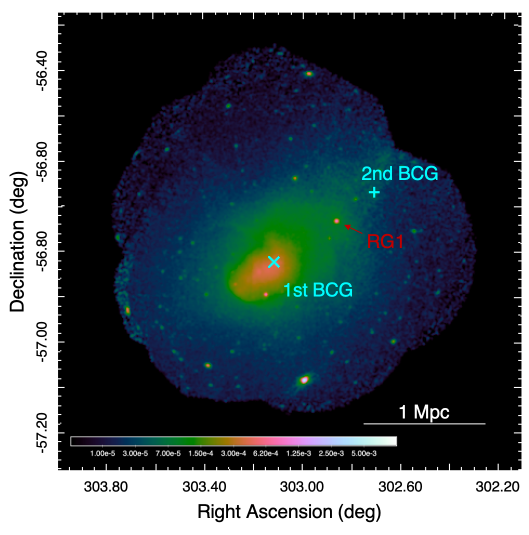
Figure 1: The exposure corrected and background subtracted image in Abell 3667 in the 0.5–7.0 keV energy band. Cyan “x” represents the positions of the 1st BCG and “+” the 2nd BCG. The pixel size is 2$\arcsec\times$2$\arcsec$.

2.2 Image and spectroscopic analysis procedure

In the image and spectroscopic analysis procedure, the event data were calibrated following the cookbook of analysis procedures for XMM–Newton EPIC. A mosaic exposure corrected and background subtracted image in the 0.5-7.0 keV energy band is shown in Figure 1. Spectral and response files were generated using the pn-spectra task and the quiescent particle background was estimated using the pn-back task. Spectral fitting was performed using xspec v12.12.0 (Arnaud 1996). The thermal emission was reproduced by the apec model with the abundance table in Lodders et al. (2009), and the redshift was fixed at 0.0556 except for the analysis of the ICM velocity measurements. The hydrogen column density was fixed at $1.40\times 10^{21}\leavevmode\nobreak\ \rm{cm^{-2}}$, determined from the HI map of the Leiden / Argentina / Bonn (LAB) survey (Kalberla et al. 2005). The sky background was separated into three components: the Local Hot Bubble (LHB), the Milky Way Halo (MWH), and the Cosmic X-ray Background (CXB). These were reproduced with the same model as described in Omiya et al. (2023), but the abundance table was changed to Lodders et al. (2009).

Table 1: The observation list in Abell 3667.

obsid	Duration	Revolution	mode
0105260101	21 ks	144	EFF
0105260201	20 ks	155	EFF
0105260301	18 ks	150	EFF
0105260401	17 ks	150	EFF
0105260501	19 ks	150	EFF
0105260601	26 ks	149	EFF
0206850101	67 ks	806	EFF

2.3 Bulk velocity measurement procedure

In the bulk velocity measurement procedure, we took three steps in the gain re-calibration, following the steps suggested by Sanders et al. (2020). The first-order correction is a time-dependent calibration of the average gain of the detector using the Cu-K$\alpha$ background line. The second order correction is a detector position dependent calibration every 500 rotations after the first correction has been applied. The third order correction is the energy scale calibration using several emission lines, including the Mn-K lines in the Filter Wheel Closed (FWC) data illuminated by the ⁵⁵Fe calibration source (hereafter CAL-FWC data). All of these data pointing to the center of Abell 3667 were observed with the Extended Full Frame (EFF) mode (Strüder et al. 2001) in the 0-1500 (2000$\sim$2008). Using observations matching these conditions, we estimated the functions of the three steps needed to re-calibrate the energy scale. The main difference from Sanders et al. (2020) is that this paper uses CAL-FWC data with only the EFF mode, while Sanders et al. (2020) uses the FF and EFF modes without distinction. Since the gain re-calibration focuses only on the energy scale correction around the Fe-K line, and the central region of the detector cannot be used, we have used this method only when measuring the bulk velocity. The details of the gain re-calibration method are described in Appendix A.

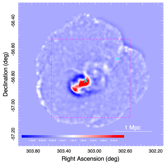
Figure 2: The unsharp masked image created by subtracting images smoothed with $\sigma$=45$\arcsec$ and $\sigma$=180$\arcsec$. The outside of the field of view shows zero values. The pixel size is 2$\arcsec\times$2$\arcsec$. The magenta rectangle indicates a field of view in Figure 3.

3 Features in ICM distribution in the central region

3.1 Tail and large vortex structures near the BCG

In Figure 1, the location of the brightest cluster galaxy (1st BCG) is indicated by a cyan “x” mark, while that of the second BCG (2nd BCG) is indicated by a cyan “+” mark (Smith et al. 2004; Piffaretti et al. 2011). The pixel size is 2$\arcsec\times$2$\arcsec$. To emphasize the gradients, we created an unsharp masked image (e.g., Fabian et al. 2006; de Plaa et al. 2012) by subtracting images smoothed with $\sigma$=180$\arcsec$ from those with $\sigma$=45$\arcsec$, as shown in Figure 2. Point sources with flux greater than 2.0$\times$10^-15 erg cm^-2 s^-1 were identified and hidden by filling with random values in the surrounding region. The left panel of Figure 3 shows the unsharp masked image focused on the cluster center overlaid with the contours of 5$\times$10^-7, 5$\times$10^-6, and 5$\times$10^-5 pixel^-1. The unsharp masked image suggests the existence of several special features in Abell 3667.

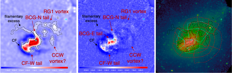
Figure 3: (Left) The same image as shown in Figure 2. It focuses on the cluster center, and the field of view indicated by the magenta rectangle in Figure 2. It is overlaid with the contours of 5$\times$10^-7, 5$\times$10^-6, and 5$\times$10^-5 pixel^-1. (Middle) The unsharp masked image created by subtracting images smoothed with $\sigma$=3$\arcsec$ and $\sigma$=60$\arcsec$, presented to show fine structures. The same image as shown in Figure 1. Red polygons indicate the region selected in the analysis of the thermodynamic and abundance maps discussed in Section 3.2. Cyan polygons indicate the region selected in the line-of-sight bulk velocity measurement discussed in Section 5.

First, the location of the cold front is confirmed at the boundary between the enhanced and diminished region to the southeast. Interestingly, the enhancement inside the cold front extends westward with a width of about 100 kpc, as if it were a tail. The edge of this “CF-W tail” also appears as a clear step in a detailed analysis of the X-ray brightness distribution in Chandra (see the 225^∘–240^∘ sector of Figure B1 in Ichinohe et al. 2017), to the best of our knowledge it is the first clear identification of this feature.

The filamentary excess extending from near the 1st BCG to the northeast is already noted in several papers, such as Vikhlinin et al. (2001a); Ichinohe et al. (2017). In our unsharp masked image, the excess of this feature is 4.2$\times$10^-6 pixel^-1 or 5.6$\sigma$, where $\sigma$=7.5$\times$10^-7 pixel^-1 is the image root mean square (rms) noise. Mazzotta et al. (2002), first mentioned this feature and suggested that it was evidence of cooler, denser gas in the cluster core being stripped out by hotter atmospheric gas. Some studies have shown that the filamentary excess has a relatively high Fe abundance, strengthening the possibility that it originates from the cluster core (Lovisari et al. 2009; Datta et al. 2014).

In the unsharp masked image, we noticed a previously unreported feature, the large clockwise vortex structure extending from the cluster center outward between the 1st and 2nd BCGs. The brightness is 10.6$\sigma$ or 8.0$\times$10^-6 pixel^-1 with respect to the rms noise. The vortex has a radius of about 250 kpc, and the structure seems to start at the 1st BCG. At the endpoint, there is a bright Radio Galaxy (B2007 -569) (Rottgering et al. 1997; Roettiger et al. 1999; Riseley et al. 2015), which is named RG1 in de Gasperin et al. (2022). The “RG1 vortex” is also visible in the XMM–Newton image in other papers (e.g., Sanders et al. 2016; Sarazin et al. 2016; Storm et al. 2018) and the Chandra image (Ichinohe et al. 2017), although not pointed out to date. This feature is connected to the 1st BCG, with a clear enhancement there, which we name the “BCG-N tail”. We also identified a counter-clockwise enhanced vortex structure with a radius of 250 kpc. The “CCW vortex” extending from the cluster center outwards has a significance of $\sigma$=5.3. However, due to the nature of unsharp masking and the relatively low significance, it is not clear whether it is the edge of the density jump, and/or the inner layer of a “dip” inside the “RG1 vortex”.

3.2 Thermodynamic and abundance maps

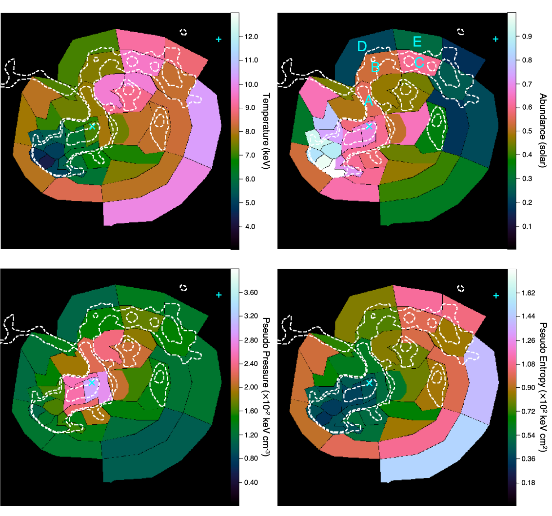
Figure 4: The thermodynamic and abundance maps with regions as indicated by the red polygons in the right panel of Figure 3. The upper-left panel shows a temperature map overlaid with white contours that are the same as the black contours in the left panel of Figure 3. The pseudo-density (upper right), pseudo-pressure (lower left), and pseudo-entropy (lower right) maps assume that the ICM is uniformly spread over the line-of-sight depth of 1 Mpc. The units of the 2D temperature, pseudo-density, pseudo-pressure, and pseudo-entropy maps are keV, $\textrm{cm}^{-3}$ $\times$ $(l/1\leavevmode\nobreak\ \textrm{Mpc})^{-1/2}$, $\textrm{keV\leavevmode\nobreak\ cm}^{-3}$ $\times$ $(l/1\leavevmode\nobreak\ \textrm{Mpc})^{-1/2}$ and $\textrm{keV\leavevmode\nobreak\ cm}^{2}$ $\times$ $(l/1\leavevmode\nobreak\ \textrm{Mpc})^{1/3}$, respectively. The cyan symbols (”x” and ”+”) represent the BCGs, the same as in Figure 1.

To explore the large vortex structures, we created two-dimensional thermodynamic and abundance maps. We have divided the regions along the enhancement or dip, as indicated by the red polygons in the right panel in Figure 3. Figure 4 shows the projected (or 2D) temperature ($kT$), metal abundance ($\Lambda$), pseudo pressure ($\bar{P}$), and “astrophysical entropy” ($\bar{S}$) maps in the regions. The $\bar{P}$ and $\bar{S}$ were calculated, using the pseudo density ($\bar{n}_{\mathrm{e}}$), as $\bar{P}=\bar{n}_{\mathrm{e}}kT$ and $\bar{S}=\bar{n}_{\mathrm{e}}^{-2/3}kT$, respectively. The $\bar{n}_{\mathrm{e}}$ was obtained from the normalization of the $\it{apec}$ model by assuming that the ICM is uniformly distributed over the line-of-sight depth of 1 Mpc, and that the electron density $\bar{n}_{\mathrm{e}}$ and the hydrogen density $\bar{n}_{\mathrm{H}}$ satisfy the relation $\bar{n}_{\mathrm{e}}=1.2\bar{n}_{\mathrm{H}}$ considering the full ionization of helium.

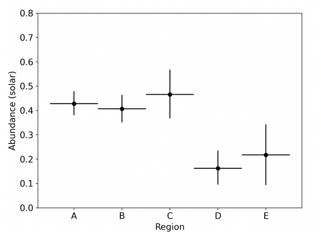
Figure 5: The abundance profile in 5 regions near the RG1 vortex with errors. The location of each region is indicated in the upper panel of Figure 4.

The RG1 vortex has high abundances comparable to the central region, while no significant pressure jump is observed. The entropy is lower towards the BCG N-tail. In Figure 5, we presented the abundance results with error bars. Regions inside the vortex (regions A, B, C, see also the upper right panel of Figure 4) have significantly higher abundance than those outside (D and E), by a factor of about 2. These results suggest that the RG1 vortex structure is the remnant ICM of the cluster core.

4 Possible scenarios for the ICM features

4.1 Karman Vortex scenario within a face-on merger

Vortex structures have been found in some clusters, but on a much smaller scale. The most prominent examples are KH rolls or vortices. Previous hydrodynamic simulations have predicted that KHI at the boundary of fluids with different densities and velocities will produce a 10-100 kpc-scale vortex in its shear layer (e.g. Heinz et al. 2003; ZuHone et al. 2010; Roediger et al. 2011; Vazza et al. 2012). In fact, the eddies have been observed in some clusters [e.g. Virgo: Werner et al. (2016), Abell 1775: Hu et al. (2021), Abell 2142: Wang & Markevitch (2018), Abell 2319: Ichinohe et al. (2021)]. In Abell 3667 the KH eddies are also indicated at the cold front boundary in the deep Chandra observations. A possible explanation for the large clockwise vortex is that these KH eddies grew in the flow into which the sub-cluster core plunged.

Several fluid dynamics studies predicted that the KH roll would move away from the shear layer, become a free vortex, and eventually form a Karman vortex sheet that aligns in a stable position (e.g. Cai et al. 2018). It is established if the Reynolds number exceeds 300 (Kiya et al. 2001). Since the Reynolds number of the ICM is $\sim$ 2100, the Karman vortex can be formed (Ichinohe et al. 2017). In addition, because the vortices of opposite sign are produced at each cycle, the rows of alternating vortices are formed on the Karman vortex sheet. It is possible that the RG1 vortex and the CCW vortex flowing from near the BCG are located at the downstream end of the Karman vortex sheet.

The vortex shedding frequency is calculated to be 0.4 Gyr^-1, assuming that the Strouhal number is 0.2 (Ichinohe et al. 2017). Abell 3667 is estimated to be about 1 Gyr after the start of the collision (Sarazin et al. 2016). In other words, a few 250–500 kpc-sized vortices can in principle form. However, it is not clear if such a large vortex can actually grow within the time scale. We will leave this scenario for future work, as it requires a wide range of numerical fluid simulations that are beyond the scope of this paper.

4.2 Offset merger scenario

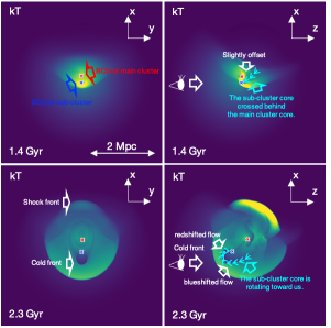
Figure 6: The projected temperature distribution in simulation in each epoch provided by the Galaxy Cluster Merger Catalog (http://gcmc.hub.yt) (ZuHone et al. 2016, 2018). The initial parameter of the mass ratio is set to 3:1. The initial impact parameter is set at 1000 kpc in the z-axis direction, and the two clusters approach each other by moving along the x-axis. The location of BCGs in the sub-cluster and main cluster is indicated by blue and red crosses, respectively. Detailed results are shown in Figure 15 in the Appendix C.

There is little doubt that Abell 3667 is a nearly head-on major merger almost within the skyplane, because this scenario can explain well the double radio relic and the relatively flat optical redshift distributions. However, it is possible that there was a small offset in the merger. This scenario is also addressed in Roettiger et al. (1999) and Sarazin et al. (2016). In such an offset merger, it is natural for the ICM to have an angular momentum to produce vortex structures while stripping each other.

4.2.1 Comparison with simulation

We compared our results with a merger simulation provided by the Galaxy Cluster Merger Catalog (http://gcmc.hub.yt) (ZuHone et al. 2016, 2018). Figure 6 shows the simulated ICM physical parameter distributions of a 3:1 mass cluster merger, which is the same condition of mass ratio as those presented in Poole et al. (2006) and Datta et al. (2014) for Abell 3667. The initial impact parameter is set to 1000 kpc in the z-axis direction (see the panels at 0 Gyr in Figure 15). The two clusters approach each other, moving along the x-axis as time passes. The simulation results show that at 1.4 Gyr there is a slight offset in the center of the cluster cores as they cross each other. The ICM in the sub-cluster is stripped from the surrounding high temperature ICM. The central remnant then rotates due to angular momentum. As the two BCGs (or the central cores of the cluster dark matter halo) begin to move back towards each other for the second encounter, the ICM will also be pulled back following the BCGs (see Figure 15).

The simulation results, as shown in Figure 15, show that the offset merger scenario can easily produce large ICM vortex structures, although their location is not the same as that of Abell 3667, which is reasonable because the simulation is not specifically performed to reproduce it. At 1.9–2.3 Gyr, when the sub-cluster is rotating, the results in the y-z plane (and the x-y plane) show sharp X-ray brightness and temperature jumps at the cold front position (see Figure 6). Therefore, the existence of sharp cold fronts and relics in Abell 3667 can also be explained in the offset merger scenario.

This scenario is also supported by the location of the 1st BCG. The 1st BCG was about 500 kpc behind the cold front in the sky plane, as shown in Figure 1. In Figure 6 and Figure 15, the positions of the BCGs in each cluster are marked with blue (1st BCG) and red (2nd BCG) crosses. As shown in Figure 15, the 1st BCG is associated with the cold front at 1.9 Gyr, but then the BCG is pulled back by the gravitational potential while the ICM in the core region is still pushed forward. The rotation of the high-density ICM on the sky plane appears as a “slingshot” structure, which is observed in several merging clusters [e.g. the Coma cluster: Lal et al. (2022); Abell 2061: Sarazin et al. (2014), ZwCl 2341+0000; Zhang et al. (2021)]. Assuming the offset merger model with rotating sub-cluster core, we can explain that the BCG was about 500 kpc behind the cold front in the sky plane, which corresponds to the simulation at 2.1–2.3 Gyr. Such a feature is also seen in another double radio relic merger, Abell 3376, where the BCG was about 170 kpc behind the cold front (Durret et al. 2013; Urdampilleta et al. 2018).

4.2.2 X-ray tail structures observed around BCG

In Section 3.1, we identified some tail structures around the 1st BCG, including the BCG-N tail. The unsharp masked image focused near the cold front, in the middle panel of Figure 3, shows that there are two tail structures associated with the 1st BCG. The “BCG-E tail” to the southeast, and the “BCG-N tail” to the north. The enhancement of the “BCG-E tail” corresponds to $\sim$ 10% of the original surface brightness. The Gaussian Gradient Magnitude (GGM) filtered images also show the existence of a similar structure (see Figure 4 in Sanders et al. 2016). Assuming that the 1st BCG is moving from the cold front to the center, the enhancement appears to trace the movement of the 1st BCG. One possibility is that it is the ISM (or the remnant of the ICM in the subcluster core) being stripped by the surrounding ICM.

The BCG-E tail can be explained by the remnant ICM of the subcluster core as well as the BCG-N tail (part of the RG1 vortex). The abundance map in Figure 4 shows that the ICMs in these regions are 0.4–0.6 solar, which is about 1.5 times higher than those of the surrounding regions. The pseudo-entropy is 2-3 times lower than the surrounding ICM, and it is comparable to the value near the cold front. These are the features seen in the cluster core.

5 Measuring the line-of-sight bulk velocity with the gain re-calibration method

The redshift of the 1st BCG is 0.0556, while the redshift of the 2nd BCG is 0.0560 (Smith et al. 2004), with a velocity difference of 120 $\pm$ 86 km s^-1, almost the same value. Then, how can we explain the coincidence of the two BCG line-of-sight velocities and their apparent alignment to the merger axis within the offset merger scenario at the same time? If the cores of the two clusters crossed and rotated almost on the sky plane, such as in the case of merging clusters with the slingshot structure, the redshift coincidence can be easily explained but not the alignment. Another possible scenario to explain the coincident redshift of the BCGs in the offset merger with an offset near the line of sight is when the individual BCGs are near the apogee of their orbital rotation after the first crossing. Since the orbital plane will be nearly on the line of sight, the apparent alignment of the orientation on the sky plane with the merger axis can also be explained. In that case, the ICM velocity in the line of sight would be dispersed because the ICM flow remains in this case. Therefore, we measured the bulk velocity distribution in the line of sight using the gain re-calibration method.

5.1 Overall ICM redshift distribution of Abell 3667

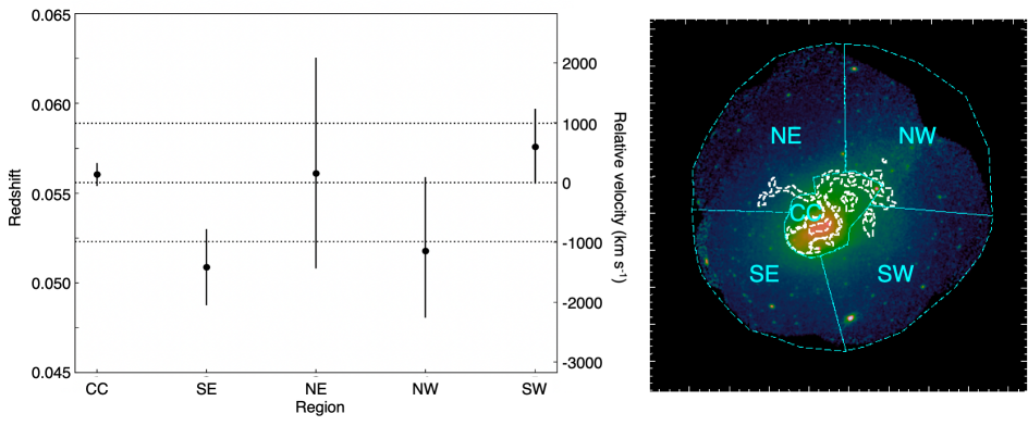
Figure 7: The result of the redshift measurement in the large regions. The region we defined is overlaid on the right panel, which is the same image as in Figure 1. The horizontal axis is the region number given in the right panel of Figure 8. The right-hand scale in the redshift distribution is the relative velocity based on the optical redshift of the 1st BCG ($z$=0.0556). As a guide, the velocity differences of $\pm$1000 km s^-1 are shown as the two dotted lines.

Before going into the details of the central portion, we present the large-scale velocity structure obtained by the gain re-calibration method. As shown in the right panel of Figure 7, the entire field of view of the data we used was divided into 5 large regions: one region at the cluster center and the other regions around it. The results are shown in Figure 7.

The redshift of region CC, located at the center of the cluster, is consistent with the optical redshift of the 1st BCG with considerable accuracy. Furthermore, the redshifts of region NE, NW, and SW are also consistent with the redshift of the 1st BCG within a 1$\sigma$ confidence interval. The consistency of these velocities suggests that the overall merging is taking place close to the skyplane. It should be noted, however, that the measured redshifts are not well constrained due to the low surface brightness.

On the other hand, region SE tends to be blueshifted compared to region CC. The relative velocity difference with respect to the optical redshift of the 1st BCG is $-$1400 $\pm$ 630 km s^-1, which means that it differs by 2.3$\sigma$. The location of this region is outside the cold front and along the merger axis. It could be explained by the large asymmetric flow generated by the sub-cluster plunge in the case of the offset merger. It could also be explained by a possible tilt of the merger axis in the case of a face-to-face merger. Thus, it is difficult to distinguish between these scenarios in the overall redshift distribution of the ICM. We note that the region coincides with the sub-group of galaxies named KMM 5 in Owers et al. (2009), which has a redshift of about $-500$ km s^-1 (i.e. blueshifted).

5.2 Central ICM redshift structures in the cluster center

As the next step, we studied the CC region in detail. Because its statistics are high, it can be divided into several sub-regions. To properly select the regions, we created the Fe-K count map. The energy range of the emission line is defined as 6.4–7.1 keV. We also define band 2 (5.7–6.4 keV) and band 3 (7.1–7.8 keV) in the same energy interval on the low and high energy sides, individually. The continuum component in band 1 was reproduced by the average count of band 2 and band 3, and the count of the Fe-K emission line was calculated by subtracting it from band 1. The ranges in band 1-3 were shifted by multiplying by 1+$z$. The results are shown in the right panel of Figure 8. As indicated by the cyan polygons, we subdivided 8 regions so that the Fe-K emission line count is 50–200 counts in each region.

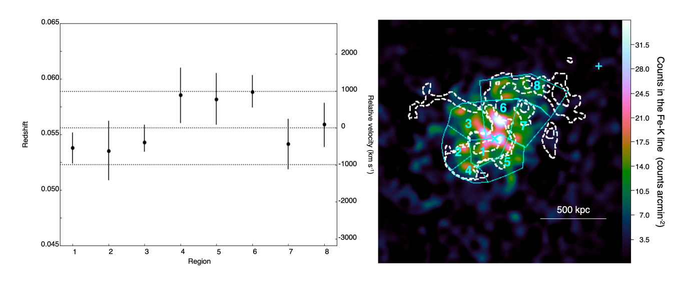
Figure 8: (Left) The result of the redshift measurement in the small regions. The horizontal axis is the region number indicated in the right panel of Figure 8. The right-hand scale in the redshift distribution is relative velocity based on the optical redshift of the 1st BCG ($z$=0.0556). As a guide, the velocity differences of $\pm$1000 km s^-1 are indicated as the two dotted lines. (Right) The count map in the FeK line. White polygons indicate the region selected for the line-of-sight bulk velocity measurement. The white contours are the same as the black contours in Figure 3.

The results of the line-of-sight bulk ICM velocity measurements in individual regions are shown in the left panel of Figure 8. The redshift in region 1, which covers the southeastern half of the 1st BCG, is consistent with that of the 1st BCG within 1.3$\sigma$ error. The redshifts in the regions between the cold front and the 1st BCG (reg 1-5) are also individually consistent within the 1.2 sigma error range. Here we performed the chi-squared test assuming that the redshift of the ICM in all regions coincides with the redshift of the BCG. The p-value was estimated to be 0.15, which is consistent with this scenario.

However, if we look at the individual values, it is noticeable that the line-of-sight velocity in region 6 is redshifted by 980 $\pm$ 440 km s^-1 and differs from that of the 1st BCG by 2.3$\sigma$ (or by $1.3$% upper-tail probability). The region is located north of the BCG and is connected to the RG1 vortex. In other words, the BCG-N tail shows a symptom of redshift.

From the left panel of Figure 8, we can see that region 2 and 3, which are located to the east of region 1 (the head of the cold front), show a tendency to be blueshifted, while region 4 and 5, which are located to the southwest, show a tendency to be redshifted. To improve the statistics, we performed a simultaneous fitting, merging the spectra of regions 2 and 3 or 4 and 5, respectively. In this case, the parameters of temperature and abundance were free in individual regions, and the parameter of redshift was constrained to have the same value. The redshift is estimated to be 5.40${}_{-0.14}^{+0.19}\times$10^-2 in region 2–3. and 5.84${}_{-0.17}^{+0.17}\times$10^-2 in region 4–5. The velocity difference between their regions is 1300 $\pm$ 860 km s^-1. The p-value, assuming that its redshift is the same as the redshift of the BCG, is estimated to be 0.03. In short, from the perspective of the cold front (region 1) looking southeast, the “right side” is blueshifted and the “left side” is redshifted.

5.3 Comparison with simulation for discussion of the merging picture

Simulation results at 2.3 Gyr in Figure 6, when the BCG reaches near apogee, show that the ICM of the central cluster rotates in an arc, bulging outward. The predicted motion of the cluster core ICM is indicated by the cyan arrows. If we were looking from the “$-$z” direction, the ICM would be blueshifted in the region near the cold front (region 1). Also, the arc-like motion of the ICM in the cluster core falling back towards the BCG (region 6) would be observed to be redshifted. If this interpretation is correct, then the sub-cluster core crossed behind the main cluster core and moved toward us, as shown in the upper right panel of Figure 6.

In this case, the BCG-N tail would appear as an enhancement of the backward motion of the ICM due to the rotation of the sub-cluster core. On the other hand, the BCG-E tail is probably the floating ISM of the 1st BCG that has been stripped off during the rotation. The redshift of regions 2,3 and 4,5, which are symmetrically located on the collision axis could be attributed to the rotation of the sub-cluster, whose axis of rotation is slightly tilted with respect to the line of sight.

Although several regions with significant line-of-sight velocity shifts were identified, our ICM velocity analysis based on XMM–Newton data could not provide clear results to unambiguously identify the merger scenario. Therefore, XRISM observations with accurate bulk and turbulence velocity measurements are essential. Velocity mapping with multiple observations around the cold front and BCG would be valuable not only for distinguishing the merger scenario in Abell 3667, but also for understanding ICM physics, such as viscosity and turbulence generation.

6 ASKAP radio observation

In recent years, many extended radio emissions have been newly detected using radio telescopes like MeerKAT (Jonas & MeerKAT Team 2016) and the Australian Square Kilometre Array Pathfinder (ASKAP) (Norris et al. 2011). The morphology of the cluster radio halo will reflect the merger geometry, and we compared the newest archival Abell 3667 observation data of ASKAP observed in August 2023 with our X-ray data. Figure 9 shows the total radio intensity map at 943 MHz with a cyan contour at 1.7 $\mu$J beam^-1.

Interestingly, the excess of radio intensity is seen in the northern direction of the BCG. Its location is consistent with that of the BCG-N tail and region 6 with a redshifted velocity in line of sight. Its symptoms are also visible in the MeerKAT image at 1.2 GHz (de Gasperin et al. 2022). If the offset merger scenario is true, it is probably evidence of particle acceleration and magnetic field enhancement by turbulence generated by the backflow of the moving sub-cluster core into the 1st BCG.

It also appears that the radio halo near the BCG elongates to the south, beyond region 4 and 5, including the “CF-W tail”. On the other hand, there is no significant feature of such a tail on the sides of region 2 and 3. The inherent asymmetry (to the cold front) in the radio band can be explained by the offset merger scenario, although an alternative explanation, such as a Karman vortex scenario, would exist. A detailed multi-wavelength radio study will be performed by Riseley et al. (in preparation).

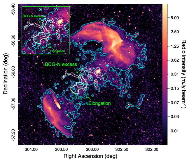
Figure 9: The radio total intensity map with the ASKAP with the cyan contour of the intensity of 1.7 $\mu$J beam^-1. Cyan crosses indicate the locations of the 1st BCG and the 2nd BCG, individually. The white contours are the same as the black ones in Figure 3. The upper left panel, enclosed by the green rectangle frame, shows the enlarged image of the center with the color bar scale magnified by a factor of 5.

7 Conclusions

In this work we revisit the ICM distribution in Abell 3667 using the image and spectroscopic analysis with the XMM–Newton data. In addition, we examined the bulk velocity distribution with the XMM–Newton EPIC-PN calibration technique using background emission lines. We have reproduced the approach shown in Sanders et al. (2020) and reproduced their results in the Coma cluster (see Appendix B) by calibrating the energy scale of the observational data with the EFF mode in 2000–2006.

In the imaging analysis, we pointed out the “RG1 vortex” for the first time, a clockwise large vortex enhancement with a radius of about 250 kpc connecting the 1st BCG and the RG1 galaxy. The structure extending northwards from the 1st BCG towards the RG1 vortex is called the “BCG-N tail”. The RG1 vortex has a high abundance of $\sim$0.5 solar, comparable to the central region, which is about twice as high as the neighboring regions. It is a symptom of the remnant ICM of the cluster core. We discussed the possible scenario that the RG1 vortex is the Karman vortex. While this is possible, detailed fluid dynamics simulations are required to actually show whether such a large vortex can form within the merger, which is beyond the scope of this paper.

Another possible scenario is the offset merger scenario. If there is even a small offset in the cluster core when their cores cross, it would be relatively easy for the mutually stripped ICMs to have angular momentum to produce vortex structures.

The newly obtained results of the line-of-sight ICM velocity measurements with the gain re-calibration method showed that region 6, which includes the BCG-N tail associated with the RG1 vortex, is redshifted by 980$\pm$440 km s^-1 of velocity difference compared to the optical redshift of the 1st BCG. The marginal dispersion in the line-of-sight velocity of the ICM supports the offset merger scenario. An enhanced ICM emission to the east of the 1st BCG, the “BCG-E tail”, has also been reconfirmed, but its origin in the offset merger scenario is not yet well understood. At this stage, the observational redshift difference results are not comprehensive, and XRISM mapping observations with accurate bulk velocities are essential.

We compared the X-ray results with the ASKAP data at 943 MHz. There is an excess of radio intensity near the BCG-N tail, which is also visible in the MeerKAT observations (de Gasperin et al. 2022). If this is consistent with the offset merger scenario, it is probably evidence for particle acceleration and magnetic field enhancement by turbulence generated in the backflow of the moving sub-cluster core into the 1st BCG. It also appears that the radio halo near the BCG is extending southward, coincident in position with the “CF-W-tail”. These asymmetric features are supportive of the offset merger scenario.

Appendix A Detail of the measuring bulk velocity procedure

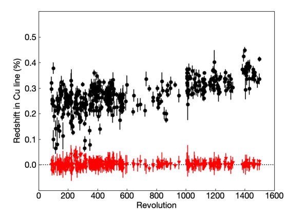
Figure 10: The redshift in the Cu–K$\alpha$ line as a function of time in revolutions from 0–1500. One revolution is $\sim$2 days. The redshift of 0.1% is about 8 eV in the Cu-K$\alpha$ line. The red markers indicate the results of the re-measurement after the first-order correction, which corrects for these redshifts by multiplying PI by 1+$z$.

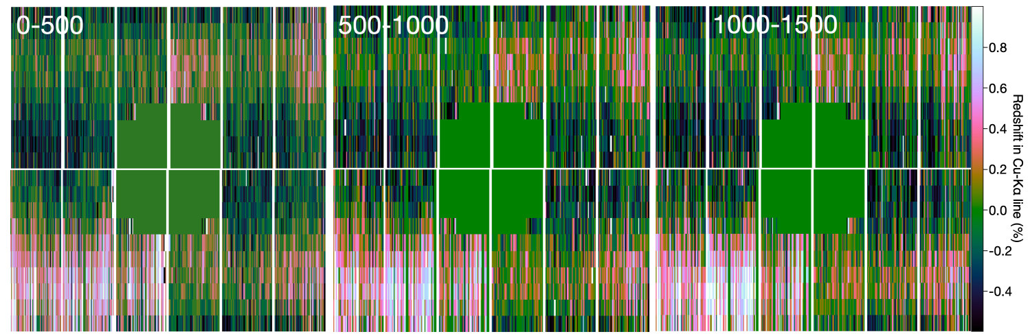
Figure 11: The redshift (in percent) in the Cu–K$\alpha$ line as a function of detector position in every 500 revolutions (0-500, 500-1000,1000-1500) after the first order correction. The spectra fitting was performed in each 1$\times$20 pixel fine region.

The EFF mode data we used were filtered to have at least 10000 counts from 7.0 to 9.25 keV to keep the statistical error in individual data as small as possible. Using these data, the gain re-calibration function was estimated in three steps. In the first-order correction, the redshift ($z$) of the Cu–K$\alpha$ line is measured in each observation and corrected to zero. The spectrum is extracted from a spatial region excluding the “Cu-hole”, which is a polygon region in the center of the detector defined by Sanders et al. (2020). We fit the spectrum in 7.0–9.25 keV with a power-law model and 4 Gaussian models (Ni–K$\alpha$, Cu–K$\alpha$, Zn–K$\alpha$, Cu–K$\beta$). The photon index of the power-law model is set to 0.136, which is an average value in Sanders et al. (2020). We used a response matrix file with an energy bin of 0.3 eV created by the rmfgen task and did not use an ancillary response file. The line energy position of the Gaussian components is left free and the sigma is fixed at 0.0. The spectrum fitting was done by C-statistic in xspec.

The redshift in the Cu–K$\alpha$ line as a function of time in each observation is shown in Figure 10. A 0.1 percent corresponds to $\sim$8 eV. We calibrated the gain shift by multiplying the PI value by 1+$z$. The results of the redshift re-measurement after first-order correction are also shown in Figure 10. Note that the similar long-term CTI using the Cu–K$\alpha$ line was already updated in May 2023 (XMM-CCF-REL-389), but we have not adopted it.

In the second-order correction, the redshift in the Cu–K$\alpha$ line depending on the detector position is measured and corrected. The first-order corrected data were stacked every 500 revolutions, i.e. divided into three time-dependent groups. The spectra in the stacked data were extracted from 1 $\times$ 20 pixel regions in each CCD. We fitted the spectra in 7.7–8.3 keV with a power-law and a Gaussian model (Cu–K$\alpha$). The fitting model is the same as that used in the first-order correction. The redshift maps in Cu–K$\alpha$ in each fine region are shown in Figure 11. Although the region size is slightly different from that of Sanders et al. (2020), our results are remarkably similar to those shown in Figure 6 of Sanders et al. (2020). In the standard calibration, the Mn–K$\alpha$ and Al–K$\alpha$ emission lines in the CAL-FWC data are used to correct the gain along the readout direction at each CCD node. There is a non-uniformity in the illumination intensity of the calibration source, which is strong between CCD4 and CCD7. The intensity around the readout nodes of CCD7 and CCD9–12 is about 200 times weaker than this region, so the calibration functions at these positions have a large redshift or blue shift in Cu-K$\alpha$. We also calibrated the stacked data by multiplying the PI value by 1+$z$.

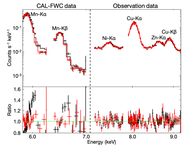
Figure 12: An example of the spectrum in the CAL-FWC data and the observation data after the second-order correction. The position of the emission line in the fitting model is fixed at the theoretical value. Red points indicate spectra with the third-order correction applied, in which the energy scale deviations are corrected by a compression model based on the Cu-K$\alpha$ line.

In the third-order correction, the energy scale is corrected using several emission lines in the observational data and CAL-FWC data applying the first-order and second-order corrections. In this turn, we define 8 regions in each CCD, divided into 4 parts in the RAWX direction (0–16,17–32,33–48,49–64) and 2 parts in the RAWY direction (0-110,110–200). In spectral fitting, we consider 6 emission line models consisting of Mn–K$\alpha$, Mn-K$\beta$, Ni-K$\alpha$, Cu-K$\alpha$, Zn-K$\alpha$, and Cu-K$\beta$ in the 5.825–6.245, 6.375-7.000, 7.170-7.795, and 7.905–9.200 keV energy bands. As an example, Figure 12 shows a spectrum in a region of CCD3 in the 0-500 revolution. The black model shows the fitting result with the emission line position fixed at the theoretical value for comparison. Based on the Cu-K$\alpha$ emission lines, it appears that the low energy emission lines are shifted to the lower energy and the high energy emission lines are shifted to the higher energy. Therefore, we constructed a gain compression model based on the Cu-K$\alpha$ emission line as described in Sanders et al. (2020). For the data points of the emission line positions obtained by the fit ($E$) versus the theoretical emission line positions ($E^{\prime}$), we performed a chi-squared fit weighted by the error of each emission line with a model of $E^{\prime}=E(1+A(E-8.04))$. The resulting correction function was used to calibrate the energy scale in each region. The red line in Figure 12 shows the result of the spectrum fitting after the third-order correction.

In spectral analysis, we selected single events (PATTERN==0) for a good energy resolution and flagged data (FLAG==0) to remove events close to bad pixels. The response matrix file is with a 0.3 eV bin generated using rmfgen task. The ancillary response file for a source model is created by arfgen task with the parameter extendedsource=extend. The background components are reproduced by a power-law model with a photon index of 0.136 and 4 Gaussian models as well as the first-order correction. We adopt the “total fitting technique” described in Sanders et al. (2020). Specifically, the spectra were added together using mathpha. and the response files were added together with a weighting factor of the numbers of counts in the 4–9.25 keV energy band using addrmf and addarf. Velocity measurements in the Coma cluster, adapting the estimated energy scale recalibration function, are in good agreement with the result of Sanders et al. (2020). The details are described in Appendix B.

Appendix B Cross-check using the Coma cluster

For comparison with the results of Sanders et al. (2020), we have measured the bulk velocity structure in the Coma cluster using our calibration function. The data used are listed in table 2. We used the data taken in the EFF mode. Therefore the observation 0153750101 was excluded. As mentioned in the data reduction, we extracted the event files in each observation using the epchain task in SAS and filtered out the soft proton effect. The events outside the Cu-hole are re-calibrated by taking 3 steps. In the first-order correction, we used the exposure time weighted redshift of the period around 100 revolutions based on the observational data. A mosaic image in the Coma cluster was shown in Figure 13. The hydrogen column density was fixed at $8.54\times 10^{19}\leavevmode\nobreak\ \rm{cm^{-2}}$, determined from the HI map. The background components are reproduced by the power-law model with the photon index 0.136 and 4 Gaussian models as well as the first-order correction.

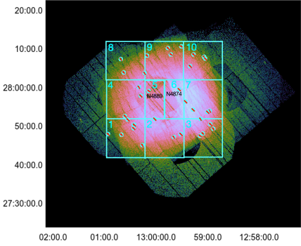
Figure 13: The mosaic count image without the Cu hole in the Coma cluster. The energy range is 0.5-10.0 keV. The rectangles in cyan show the examined regions, which were divided according to Sanders et al. (2020). The circles indicate the point sources excluded in our analysis.

A mosaic count image without the Cu hole in the Coma cluster is shown in Figure 13. As with the Sanders et al. (2020) results, we divided the Coma cluster into 10 regions as shown in Figure 13. In the spectra analysis we excluded the point sources, which are shown as circles with a radius of 30 arcsec. Figure 14 shows the bulk velocity distribution using our calibration function, overlapping the results of Sanders et al. (2020). Our results reproduce their results with good reproducibility.

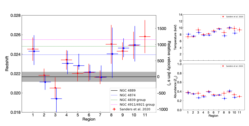
Figure 14: The result of redshift (left), temperature (lower-right), and abundance (upper-right) in the Coma cluster, comparing the result of Sanders et al. (2020). The right axis in the redshift distribution shows relative velocity based on the redshift of NGC 4889 (z=0.0217).

Table 2: The observation list in the Coma cluster.

obsid	Duration	Revolution	mode
0124710501	30 ks	86	EFF
0124710601	32 ks	93	EFF
0124710901	31 ks	93	EFF
0124711401	35 ks	86	EFF
0124712001	23 ks	184	EFF
0300530101	26 ks	1012	EFF
0300530201	28 ks	1011	EFF
0300530301	31 ks	1008	EFF
0300530401	28 ks	1007	EFF
0300530601	26 ks	1006	EFF
0300530701	26 ks	1006	EFF

Appendix C Detail of the offset merger simulation

Figure 15 shows the result of a 3:1 mass cluster merger simulation with an initial impact parameter of 1000 kpc provided by the Galaxy Cluster Merger Catalog (http://gcmc.hub.yt) (ZuHone et al. 2016, 2018), as noted in Section4.2.1.

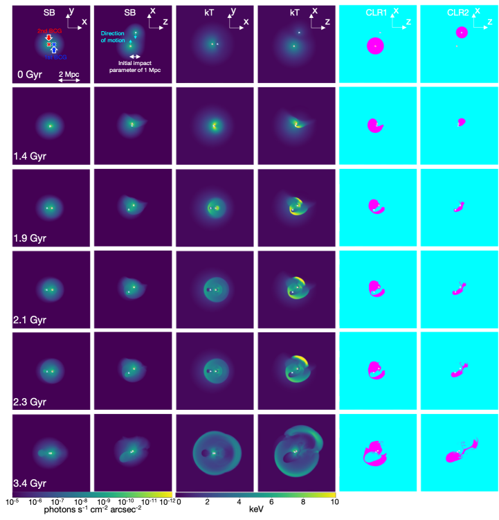
Figure 15: The simulation results of the merging cluster with an initial parameter of mass ratio of 3:1 in each epoch (0 Gyr, 1.4 Gyr, 1.9 Gyr, 2.3 Gyr, and 3.4 Gyr) provided by the Galaxy Cluster Merger Catalog (http://gcmc.hub.yt) (ZuHone et al. 2016, 2018). The initial impact parameter is set to 1000 kpc in the z-axis direction, and the two clusters approach each other by moving along the x-axis. From the left panel to the right panel: X-ray surface brightness observed from the +z-axis direction, the +y-axis direction, the projected temperature observed from the +z-axis direction, the +y-axis direction, and the Coronal-Line Region (CLR) of the main cluster and the sub-cluster from the +y-axis direction, respectively. The position of the BCG in each cluster is marked with blue and red crosses.

References

- Akamatsu & Kawahara (2013) Akamatsu, H. & Kawahara, H. 2013, PASJ, 65, 16
- Akamatsu et al. (2012) Akamatsu, H., Takizawa, M., Nakazawa, K., et al. 2012, PASJ, 64, 67
- Arnaud (1996) Arnaud, K. A. 1996, in Astronomical Society of the Pacific Conference Series, Vol. 101, Astronomical Data Analysis Software and Systems V, ed. G. H. Jacoby & J. Barnes, 17
- Asai et al. (2005) Asai, N., Fukuda, N., & Matsumoto, R. 2005, Advances in Space Research, 36, 636
- Ascasibar & Markevitch (2006) Ascasibar, Y. & Markevitch, M. 2006, ApJ, 650, 102
- Botteon et al. (2022) Botteon, A., Shimwell, T. W., Cassano, R., et al. 2022, A&A, 660, A78
- Brunetti & Lazarian (2007) Brunetti, G. & Lazarian, A. 2007, MNRAS, 378, 245
- Brunetti et al. (2001) Brunetti, G., Setti, G., Feretti, L., & Giovannini, G. 2001, MNRAS, 320, 365
- Cai et al. (2018) Cai, D., Lembège, B., Hasegawa, H., & Nishikawa, K. I. 2018, Journal of Geophysical Research (Space Physics), 123, 10,158
- Datta et al. (2014) Datta, A., Schenck, D. E., Burns, J. O., Skillman, S. W., & Hallman, E. J. 2014, ApJ, 793, 80
- de Gasperin et al. (2022) de Gasperin, F., Rudnick, L., Finoguenov, A., et al. 2022, A&A, 659, A146
- de Plaa et al. (2012) de Plaa, J., Zhuravleva, I., Werner, N., et al. 2012, A&A, 539, A34
- Dennis & Chandran (2005) Dennis, T. J. & Chandran, B. D. G. 2005, ApJ, 622, 205
- Dietl et al. (2024) Dietl, J., Pacaud, F., Reiprich, T. H., et al. 2024, arXiv e-prints, arXiv:2401.17281
- Duchesne et al. (2021) Duchesne, S. W., Johnston-Hollitt, M., Bartalucci, I., Hodgson, T., & Pratt, G. W. 2021, PASA, 38, e005
- Durret et al. (2013) Durret, F., Perrot, C., Lima Neto, G. B., et al. 2013, A&A, 560, A78
- Fabian et al. (2006) Fabian, A. C., Sanders, J. S., Taylor, G. B., et al. 2006, MNRAS, 366, 417
- Finoguenov et al. (2010) Finoguenov, A., Sarazin, C. L., Nakazawa, K., Wik, D. R., & Clarke, T. E. 2010, ApJ, 715, 1143
- Fujita et al. (2004) Fujita, Y., Matsumoto, T., & Wada, K. 2004, ApJ, 612, L9
- Fujita et al. (2003) Fujita, Y., Takizawa, M., & Sarazin, C. L. 2003, ApJ, 584, 190
- Gaspari & Churazov (2013) Gaspari, M. & Churazov, E. 2013, A&A, 559, A78
- Gatuzz et al. (2022a) Gatuzz, E., Sanders, J. S., Canning, R., et al. 2022a, MNRAS, 513, 1932
- Gatuzz et al. (2023a) Gatuzz, E., Sanders, J. S., Dennerl, K., et al. 2023a, MNRAS, 520, 4793
- Gatuzz et al. (2023b) Gatuzz, E., Sanders, J. S., Dennerl, K., et al. 2023b, MNRAS, 522, 2325
- Gatuzz et al. (2022b) Gatuzz, E., Sanders, J. S., Dennerl, K., et al. 2022b, MNRAS, 511, 4511
- Ha et al. (2018) Ha, J.-H., Ryu, D., & Kang, H. 2018, ApJ, 857, 26
- Heinz et al. (2003) Heinz, S., Churazov, E., Forman, W., Jones, C., & Briel, U. G. 2003, MNRAS, 346, 13
- Hitomi Collaboration et al. (2016) Hitomi Collaboration, Aharonian, F., Akamatsu, H., et al. 2016, Nature, 535, 117
- Hu et al. (2021) Hu, D., Xu, H., Zhu, Z., et al. 2021, ApJ, 913, 8
- Ichinohe et al. (2021) Ichinohe, Y., Simionescu, A., Werner, N., Markevitch, M., & Wang, Q. H. S. 2021, MNRAS, 504, 2800
- Ichinohe et al. (2017) Ichinohe, Y., Simionescu, A., Werner, N., & Takahashi, T. 2017, MNRAS, 467, 3662
- Jaffe (1977) Jaffe, W. J. 1977, ApJ, 216, 212
- Jonas & MeerKAT Team (2016) Jonas, J. & MeerKAT Team. 2016, in MeerKAT Science: On the Pathway to the SKA, 1
- Kalberla et al. (2005) Kalberla, P. M. W., Burton, W. B., Hartmann, D., et al. 2005, A&A, 440, 775
- Kelley et al. (2016) Kelley, R. L., Akamatsu, H., Azzarello, P., et al. 2016, in Society of Photo-Optical Instrumentation Engineers (SPIE) Conference Series, Vol. 9905, Space Telescopes and Instrumentation 2016: Ultraviolet to Gamma Ray, ed. J.-W. A. den Herder, T. Takahashi, & M. Bautz, 99050V
- Kiya et al. (2001) Kiya, M., Ishikawa, H., & Sakamoto, H. 2001, Journal of Wind Engineering and Industrial Aerodynamics, 89, 1219, bluff Body Aerodynamics and Applications
- Kurahara et al. (2023) Kurahara, K., Akahori, T., Kale, R., et al. 2023, PASJ, 75, S138
- Lal et al. (2022) Lal, D. V., Lyskova, N., Zhang, C., et al. 2022, ApJ, 934, 170
- Lodders et al. (2009) Lodders, K., Palme, H., & Gail, H. P. 2009, Landolt Börnstein, 4B, 712
- Lovisari et al. (2009) Lovisari, L., Kapferer, W., Schindler, S., & Ferrari, C. 2009, A&A, 508, 191
- Markevitch (1996) Markevitch, M. 1996, ApJ, 465, L1
- Markevitch et al. (2004) Markevitch, M., Gonzalez, A. H., Clowe, D., et al. 2004, ApJ, 606, 819
- Markevitch et al. (2000) Markevitch, M., Ponman, T. J., Nulsen, P. E. J., et al. 2000, ApJ, 541, 542
- Markevitch et al. (1999) Markevitch, M., Sarazin, C. L., & Vikhlinin, A. 1999, ApJ, 521, 526
- Markevitch & Vikhlinin (2007) Markevitch, M. & Vikhlinin, A. 2007, Phys. Rep, 443, 1
- Mazzotta et al. (2002) Mazzotta, P., Fusco-Femiano, R., & Vikhlinin, A. 2002, ApJ, 569, L31
- Nagai et al. (2007) Nagai, D., Kravtsov, A. V., & Vikhlinin, A. 2007, ApJ, 668, 1
- Nakazawa et al. (2009) Nakazawa, K., Sarazin, C. L., Kawaharada, M., et al. 2009, PASJ, 61, 339
- Norman & Bryan (1999) Norman, M. L. & Bryan, G. L. 1999, in The Radio Galaxy Messier 87, ed. H.-J. Röser & K. Meisenheimer, Vol. 530, 106
- Norris et al. (2011) Norris, R. P., Hopkins, A. M., Afonso, J., et al. 2011, PASA, 28, 215
- Ogrean et al. (2013) Ogrean, G., Brüggen, M., Simionescu, A., et al. 2013, Astronomische Nachrichten, 334, 342
- Omiya et al. (2023) Omiya, Y., Nakazawa, K., Matsushita, K., et al. 2023, PASJ, 75, 37
- Ota & Yoshida (2016) Ota, N. & Yoshida, H. 2016, PASJ, 68, S19
- Owers et al. (2009) Owers, M. S., Couch, W. J., & Nulsen, P. E. J. 2009, ApJ, 693, 901
- Petrosian (2001) Petrosian, V. 2001, ApJ, 557, 560
- Piffaretti et al. (2011) Piffaretti, R., Arnaud, M., Pratt, G. W., Pointecouteau, E., & Melin, J. B. 2011, A&A, 534, A109
- Poole et al. (2006) Poole, G. B., Fardal, M. A., Babul, A., et al. 2006, MNRAS, 373, 881
- Rajpurohit et al. (2022) Rajpurohit, K., van Weeren, R. J., Hoeft, M., et al. 2022, ApJ, 927, 80
- Rasia et al. (2006) Rasia, E., Ettori, S., Moscardini, L., et al. 2006, MNRAS, 369, 2013
- Riseley et al. (2022) Riseley, C. J., Bonnassieux, E., Vernstrom, T., et al. 2022, MNRAS, 515, 1871
- Riseley et al. (2015) Riseley, C. J., Scaife, A. M. M., Oozeer, N., Magnus, L., & Wise, M. W. 2015, MNRAS, 447, 1895
- Roediger et al. (2011) Roediger, E., Brüggen, M., Simionescu, A., et al. 2011, MNRAS, 413, 2057
- Roediger et al. (2015) Roediger, E., Kraft, R. P., Nulsen, P. E. J., et al. 2015, ApJ, 806, 104
- Roettiger et al. (1999) Roettiger, K., Burns, J. O., & Stone, J. M. 1999, ApJ, 518, 603
- Rottgering et al. (1997) Rottgering, H. J. A., Wieringa, M. H., Hunstead, R. W., & Ekers, R. D. 1997, MNRAS, 290, 577
- Russell et al. (2010) Russell, H. R., Sanders, J. S., Fabian, A. C., et al. 2010, MNRAS, 406, 1721
- Sanders et al. (2020) Sanders, J. S., Dennerl, K., Russell, H. R., et al. 2020, A&A, 633, A42
- Sanders et al. (2016) Sanders, J. S., Fabian, A. C., Russell, H. R., Walker, S. A., & Blundell, K. M. 2016, MNRAS, 460, 1898
- Sarazin et al. (2014) Sarazin, C., Hogge, T., Chatzikos, M., et al. 2014, in The X-ray Universe 2014, ed. J.-U. Ness, 181
- Sarazin (2002) Sarazin, C. L. 2002, in Astrophysics and Space Science Library, Vol. 272, Merging Processes in Galaxy Clusters, ed. L. Feretti, I. M. Gioia, & G. Giovannini, 1–38
- Sarazin et al. (2016) Sarazin, C. L., Finoguenov, A., Wik, D. R., & Clarke, T. E. 2016, arXiv e-prints, arXiv:1606.07433
- Sato et al. (2023) Sato, K., Uchida, Y., & Ishikawa, K. 2023, arXiv e-prints, arXiv:2303.01642
- Smith et al. (2004) Smith, R. J., Hudson, M. J., Nelan, J. E., et al. 2004, AJ, 128, 1558
- Storm et al. (2018) Storm, E., Vink, J., Zandanel, F., & Akamatsu, H. 2018, MNRAS, 479, 553
- Strüder et al. (2001) Strüder, L., Briel, U., Dennerl, K., et al. 2001, A&A, 365, L18
- Tamura et al. (2014) Tamura, T., Yamasaki, N. Y., Iizuka, R., et al. 2014, ApJ, 782, 38
- Tashiro et al. (2020) Tashiro, M., Maejima, H., Toda, K., et al. 2020, in Society of Photo-Optical Instrumentation Engineers (SPIE) Conference Series, Vol. 11444, Space Telescopes and Instrumentation 2020: Ultraviolet to Gamma Ray, ed. J.-W. A. den Herder, S. Nikzad, & K. Nakazawa, 1144422
- Urdampilleta et al. (2018) Urdampilleta, I., Akamatsu, H., Mernier, F., et al. 2018, A&A, 618, A74
- van Weeren et al. (2019) van Weeren, R. J., de Gasperin, F., Akamatsu, H., et al. 2019, Space Sci. Rev., 215, 16
- van Weeren et al. (2011) van Weeren, R. J., Intema, H. T., Röttgering, H. J. A., Brüggen, M., & Hoeft, M. 2011, Mem. Soc. Astron. Italiana, 82, 569
- van Weeren et al. (2012) van Weeren, R. J., Röttgering, H. J. A., Rafferty, D. A., et al. 2012, A&A, 543, A43
- Vazza et al. (2012) Vazza, F., Roediger, E., & Brüggen, M. 2012, A&A, 544, A103
- Vikhlinin et al. (2001a) Vikhlinin, A., Markevitch, M., & Murray, S. S. 2001a, ApJ, 551, 160
- Vikhlinin et al. (2001b) Vikhlinin, A., Markevitch, M., & Murray, S. S. 2001b, ApJ, 549, L47
- Wang & Markevitch (2018) Wang, Q. H. S. & Markevitch, M. 2018, ApJ, 868, 45
- Werner et al. (2016) Werner, N., ZuHone, J. A., Zhuravleva, I., et al. 2016, MNRAS, 455, 846
- Willson (1970) Willson, M. A. G. 1970, MNRAS, 151, 1
- XRISM Science Team (2020) XRISM Science Team. 2020, arXiv e-prints, arXiv:2003.04962
- Zhang et al. (2021) Zhang, X., Simionescu, A., Stuardi, C., et al. 2021, A&A, 656, A59
- ZuHone et al. (2016) ZuHone, J. A., Kowalik, K., Ohman, E., Lau, E., & Nagai, D. 2016, arXiv e-prints, arXiv:1609.04121
- ZuHone et al. (2018) ZuHone, J. A., Kowalik, K., Öhman, E., Lau, E., & Nagai, D. 2018, ApJS, 234, 4
- ZuHone et al. (2010) ZuHone, J. A., Markevitch, M., & Johnson, R. E. 2010, ApJ, 717, 908